Embed Size (px)
Citation preview

Development of a CAN Based Electric Vehicle Control System
By
Stephen A. Vincent
Submitted to the graduate degree program in Mechanical Engineering and the Graduate Faculty
of the University of Kansas in partial fulfillment of the requirements for the degree of Master of
Science.
________________________________
Chairperson Dr. Terry Faddis
________________________________
Dr. Lorin Maletsky
________________________________
Dr. Bedru Yimer
Date Defended: June 24, 2014

1
The Thesis Committee for Stephen A. Vincent
certifies that this is the approved version of the following thesis:
Development of a CAN Based Electric Vehicle Control System
________________________________
Chairperson Dr. Terry Faddis
Date approved: June 24, 2014

2
Abstract
The Intelligent Systems and Automation Lab (ISAL) at the University of Kansas has
been working on developing new electric vehicle drivetrain and battery technology using an
electric bus as a development platform. In its preexisting state the bus featured an unreliable
control system to manage load control and drive enable functions. As a result this thesis presents
the design of a Controller Area Network (CAN) based control system to be used as a
replacement for the existing system. The use of this new system will allow for easy expansion,
higher efficiency and greater reliability in further developing the ISAL electric bus concept
vehicle.
Controller Area Network protocol allows the system to easily implement smart features
allowing multiple modules to work together as well as reduce the overall wiring complexity of
the control system. CAN networks utilize a single twisted pair cable and differential
transmission to reliably transmit data to all modules featured in the control system. Additionally,
because CAN is a common network protocol used in automotive electronics it will be easy to
interface with other existing automotive electronics.
This thesis shows the development of six different CAN modules as well as a proposed
implementation for the complete system. Developed modules include an Interior Lighting
Module, Headlights and Accessories Load Module, Accelerator Pedal Sensor Module, Battery
Voltage Sensor Module, Input Module, and Speed Sensor and Display Module. Modules serve
the purpose of reading sensors, controlling electric loads and displaying pertinent information to
the driver. A prototype of this system featuring one of each module has been created for display
and test purposes and is fully functional.

3
1.0 Project History/Background
Electric vehicles have briefly emerged throughout history several times only to return
back to relative obscurity. Low expectations for range combined with the lack of reliability
accompanying early steam and gasoline powered vehicles helped electric vehicles gain
popularity during the early 1900s [1]. Later improvements in gasoline vehicle performance
along with increased reliability resulted in a sharp decline of electric vehicle popularity. Much
later, in the 1960s, interest in electric vehicles re-emerged due to rising oil prices and concerns
about the output of harmful emissions from gasoline powered vehicles. Later regulations
required percentages of vehicle sales to include zero-emission vehicles. Once again low
performance, particularly range, resulted in the failure of the electric vehicle to grab a legitimate
market share. In recent years battery technology has advanced to a point where electric vehicles
have respectable ranges and low charging times [2]. Emergence of new battery technology along
with the commercially successful Tesla model S have shown that electric vehicle technology
may have finally reached a point where it can become a commercially viable alternative to
gasoline powered automobiles. As a result the University of Kansas Intelligent Systems and
Automation Lab is working to help benchmark and improve electric vehicle efficiency using
their electric bus concept. My contribution is the development and testing of a Controller Area
Network based electric vehicle control system composed of six different networkable modules.
Many don't realize that during the infancy of automobiles there was a time when electric
vehicles were a prominent alternative to gasoline and steam powered options. In 1900 there
were 4,192 vehicles produced in the United States, 28% featured an electric-powered drivetrain
[1]. That same year at the New York Auto Show there were more electric vehicles on display
than any other type of vehicle. This popularity increased until electric vehicle production peaked

4
in 1913 followed by a rapid decline [1]. Refinement of the once clunky internal combustion
engine coupled with a desire for increased range and speed provided gasoline powered
automobiles with a meteoric rise in popularity [2]. Refueling gasoline powered vehicles was
also relatively simple compared to operating the expensive, difficult to use charging setups
available for electric vehicles at that time. Many early electric vehicles relied on custom
charging setups that were often run only by electricians [1]. By 1920 the electric vehicle was
mostly dead, with the exception of a few niche markets.
Increasing gasoline prices along with increased concerns about vehicle emissions led to a
resurgence in interest toward electric vehicles. Many electric vehicles being developed at the
time were simply electric conversions of existing gasoline powered vehicles. In the mid 1960’s
both General Motors and Ford began developing purpose built electric vehicles in an effort to
increase performance. While much higher performance than their predecessors, these vehicles
still failed to come anywhere close to the performance of a gasoline powered automobile [2]. A
1990 California Air Resources Board (CARB) regulation called for 2% of light duty vehicles
produced by manufactures selling 35,000 automobiles or more per year to be zero emission
vehicles [3]. As a result major automakers began developing electric vehicles including the
General Motors EV1, Ford TH!NK City, Nissan Hypermini, and Toyota RAV4 Electric [2].
Even these vehicles suffered from poor performance when compared to a gasoline powered
vehicle. In 1996 when General Motors delivered the first of their EV1 mass-produced electric
vehicles the maximum range was only 90 miles [3]. As a result, this new round of electric
vehicles, most of which were relatively expensive, sold poorly and considered by many to be a
failure.

5
Recent technological developments, including high energy density lithium ion battery
packs, and high efficiency drivetrains have brought electric vehicle performance to a level that
many feel could make them a successful alternative to gasoline powered vehicles. The 2006
announcement of the Tesla Roadster, which would go on sale in 2008, showed just how far
electric vehicle performance had improved. With a US EPA stated range of 244 miles and the
ability to go from 0 to 60 miles per hour in 3.7 seconds the performance was on par or exceeding
that of many gasoline powered sports cars. Additionally, a range of 244 miles exceeds that of
the average commuter’s daily drive limiting the owner’s range-anxiety. The release of several
high performance electric cars, along with renewed government interest in electric vehicles, has
sparked further research in developing electric vehicle technology. The University of Kansas has
been working to develop and benchmark new battery and drivetrain technologies using its
Electric Bus concept vehicle. As part of that system, I developed and tested a networked smart
control system designed to increase reliability and efficiency of all peripherals and parasitic
loads. Specifically, the system I developed contains the six networkable modules discussed in
this thesis.
2.0 CAN Protocol Overview
Most vehicles feature a number of different electronics modules which need to be
networked for the vehicle to operate properly. Prior to development of the Controller Area
Network (CAN), bus modules generally featured individual connections to every other module
with which they interfaced. CAN bus was developed by Robert Bosch in the mid 1980’s [4] to
replace car networks with a simpler, lower weight and lower cost alternative. Using a CAN bus
network every module can be networked to every other module with only a single connection to
a common twisted pair connection terminated at either end with 120 ohm resistors [5].

6
Prior to the development of CAN bus, modules often had a wired connection to every
single module that they communicated with. The result of this was often complex, heavy wiring
harnesses and large amounts of processing power dedicated strictly to communication. Figures
2.1 and 2.2 show the wiring simplification offered in this control system. Simplification would
be even greater in many electrical vehicles because of the large number of modules that must
interface with each other.
Figure 2.1: Wiring Diagram without Controller Area Network

7
Figure 2.2: Wiring Diagram with Controller Area Network
Standard serial communication typically sends a digital high state of 3.3 V or 5 V for a 1
and a digital low state of 0v for a 0. Over long distances this can be affected negatively by
electrical noise, which is frequently present in vehicles. CAN bus utilizes a differential pair that
monitors the difference between the state of a twisted pair of wires. Since it is likely that
electrical noise will affect both wires in the twisted pair equally the differential between them is
likely to be affected less by electrical noise. In particular CAN bus uses a differential system
where a 1 is sent when the twisted pair is in the recessive state and a 0 is sent when the pair is in
the dominant state. The recessive state occurs when both the high and low side of the CAN bus
are at a 2.5 V potential (Fig. 2.3). A dominant state occurs with a 3.3 V CAN transceiver when

8
the voltage of the high side of the bus is at 3.5v and the low side is at 1.5v creating a 2v
differential between the high and low side [6]. In a differential system if electrical noise causes
both voltages to either go up or down the difference between them will still remain the same and
the transmission will not be altered.
Figure 2.3: Differential Signal Voltages [6]
CAN networks operating in high speed mode are also capable of transmitting data up to 1
Mbit/second if the bus length is 40 meters or less [5]. CAN networks are also capable of error
checking and can feature a high number of nodes due to their 11 bits of data available for CAN
IDs [4].
In addition to simplified wiring, CAN bus networks are message based and therefore
every message is simply transmitted to the CAN bus rather than a specifically addressed module.
A benefit of this is that every module attached to the CAN bus is capable of receiving messages
from every other module attached to the bus. A result of this is a system that’s much simpler to
upgrade and add features to without the addition of complicated wiring. Modules must then
determine whether or not to discard or use each message that they receive [4]. This makes it

9
particularly easy to send sensor data to a number of different modules as well as implement
several identical modules. The control system designed for this thesis employs multiple interior
lighting modules all of which are identical in hardware and software and react to the same
messages sent over the CAN bus.
According to the CAN protocol each message must contain certain data and structure as
seen in figure 2.4.
SOF 11 bit
CAN
ID
RTR IDE R0 DLC Data CRC ACK EOF IFS
Table 2.1: CAN Message Structure
SOF: (1 bit) Start of Frame bit signals the start of a frame by first sending dominant bit. This bit
helps all of the modules synchronize after being in an idle state
11 bit CAN ID: (11 bits) binary identifier. Lower values have a higher priority
RTR: (1 bit): Remote Transmission Request. This bit is dominant when information is needed
from another node
IDE: (1 bit): Identifier extension
R0: (1 bit) Reserved bit: this is reserved for possible future amendments to the standard
DLC: (4 bits) Data Length Code: this is a 4 bit number that establishes how many bits of data
will be transmitted
DATA: (8 bits) The 8 bits of data transferred to the bus are stored here.

10
CRC: (16 bits) Cyclic Redundancy Check, this contains a checksum of preceding application
data for error detection
ACK: (2 bits) this contains an acknowledgement bit and a delimiter bit. When the original
message is sent the first bit is sent as recessive. When each node receives the message if
properly received, it will overwrite this bit with a dominant bit. This verifies the integrity of data
sent over the CAN bus.
EOF: (7 bits) These 7 bits mark the end of frame of communication
IFS: (7 bits) These 7 bits are known as the inter-frame space. They provide the necessary time
for a can controller to move the next message into the buffer. [5]
Most microcontrollers are not capable of directly interfacing with a CAN bus network.
Microcontrollers with integrated CAN controllers do exist, however for this system a standalone
CAN controller was used. The purpose of a CAN controller is to act as an interface with the
microcontroller that will utilize the CAN message protocol, store messages and determine when
to accept and reject messages on the CAN bus. Utilizing a CAN controller frees up
microcontroller resources for other functions rather than CAN implementation. This system uses
the Microchip MCP2515 Can controller IC [7] as its CAN controller which is connected to the
CAN bus through a Texas Instruments SN65HVD230 CAN transceiver IC [8] (Figure 2.5). A
CAN transceiver allows the CAN controller to send data over a differential bus helping to reduce
the effects of noise on transmission. The SN65HVD230 3.3 V transceiver was used over a 5v
transceiver due to its ability to reduce node power by as much as 50% [6].

11
Figure 2.5: Example System Implementation [7]
Since each module only requires a connection to a 9-16v DC power supply as well as a
connection to the CAN bus, module placement is much more flexible than with an analog
system. In order to reduce the amount of overall wiring, modules are placed near components
that they interface with as can be seen in figure 2.6 and Table 2.1
Figure 2.6: Bus Node Layout

12
Node # Node Name
1 Headlights and Accessories Module #1
2 Headlights and Accessories Module #2
3 Accelerator Pedal Sensor Module
4 Speed Sensor/Display Module
5 Input Module
6 Interior Lighting Module #1
7 Interior Lighting Module #2
8 Interior Lighting Module #3
9 Battery Voltage Sensor Module
10 Headlights and Accessories Module #3
Table 2.2: Module Allocation
3.0 Interior Lighting Module

13
Figure 3.1: Interior Lights Module
3.1 Interior Lighting Module Overview
Interior lighting is facilitated by CAN bus networked MCU controlled modules (Fig. 3.1).
Each module is capable of powering up to three one watt high-intensity LEDs connected in
series. This system is much more efficient than the bus’s preexisting fluorescent lighting system.
In addition to offering much higher efficiency this interior lighting module offers greater
functionality over the preexisting system due to its CAN bus connectivity. System connectivity
can be seen in the flowchart featured in figure 3.2.

14
Figure 3.2: Interior Lighting Module Flowchart
3.2 Interior Lighting Module Architecture
The LED driver used in this system is powered by a Macroblock MBI6651 Constant
Current Step-Down LED driver integrated circuit [9]. Each integrated circuit can be used with
anywhere from 1-6 LEDs and features dimming capabilities controlled via pulse width
modulation at either a 3.3 V or 5 V logic level. Each Macroblock IC is placed on the underside
of a pre-configured LED module and is configured using the schematic shown in figure 3.3.
Figure 3.3: LED Driver Schematic
Using the configuration shown in Figure 3.3 the driver will output a constant current of
370 ma making it suitable for use with 1 watt high intensity LEDs. The module itself is capable
of driving up to six of these LEDs , however when operating with an input voltage of 12 V it is

15
limited to three LEDs per module. Since each 1 watt LED is capable of outputting 90 lumens at
full brightness [10] a system with six of these modules will provide nearly the same level of light
as the previous fluorescent lighting system.
3.3 Comparison with Preexisting Lighting System
The preexisting system featured on the bus contained three fluorescent light fixtures on
each side of the bus totaling six fixtures as seen in figure 3.4.
Figure 3.4: Preexisting Light Fixture Placement
16
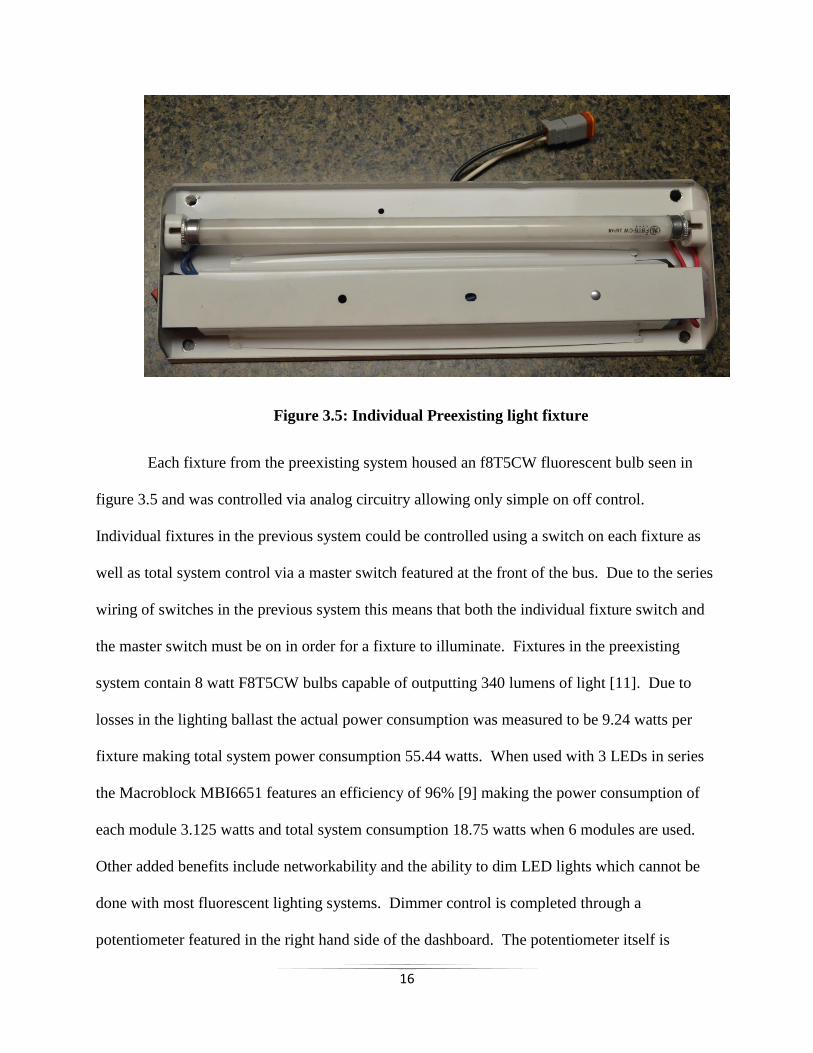
Figure 3.5: Individual Preexisting light fixture
Each fixture from the preexisting system housed an f8T5CW fluorescent bulb seen in
figure 3.5 and was controlled via analog circuitry allowing only simple on off control.
Individual fixtures in the previous system could be controlled using a switch on each fixture as
well as total system control via a master switch featured at the front of the bus. Due to the series
wiring of switches in the previous system this means that both the individual fixture switch and
the master switch must be on in order for a fixture to illuminate. Fixtures in the preexisting
system contain 8 watt F8T5CW bulbs capable of outputting 340 lumens of light [11]. Due to
losses in the lighting ballast the actual power consumption was measured to be 9.24 watts per
fixture making total system power consumption 55.44 watts. When used with 3 LEDs in series
the Macroblock MBI6651 features an efficiency of 96% [9] making the power consumption of
each module 3.125 watts and total system consumption 18.75 watts when 6 modules are used.
Other added benefits include networkability and the ability to dim LED lights which cannot be
done with most fluorescent lighting systems. Dimmer control is completed through a
potentiometer featured in the right hand side of the dashboard. The potentiometer itself is

17
connected to the input module through an 8 bit analog to digital converter which outputs a digital
value between 0 and 255 corresponding to the duty level of the interior lighting system between
0% and 100% respectively. Since each light module is capable of being networked and activated
via the CAN bus the system can easily be expanded to different numbers of modules. The only
connections necessary for additional modules are a 12 volt DC power source and the ability to
connect to the CAN bus network. Smart functions can also be programmed to trigger the lights
on or off using other sensors and inputs of the control system. A great example would be turning
the interior lights on and off based on the state of the door position. Rather than requiring
additional sensors and circuitry, a function like this can simply be added through additional
program code. Superior performance is also seen in the form of reduced maintenance. Each of
the 1 watt LEDs used in this system are rated for 50,000 [10] hours of use which far exceeds the
7500 hour [11] lifespan of fluorescent bulbs used in the preexisting system.
4.0 Headlights and Accessories Load Module

18
Figure 4.1: Headlights and Accessories Module
4.1 Headlights and Accessories Module Overview
Electric vehicles require a number of auxiliary features both for convenience and in order
to meet legal driving requirements. Front exterior lighting and accessories are controlled by two
Headlights and Accessories Load modules (Fig. 4.1) located in the front panel of the bus. An
additional module, located in the rear of the bus, controls the rear exterior lights. All of the
modules feature CAN bus network connectivity allowing easy interaction between modules with
only a single twisted pair connection. Network connectivity between modules also allows for
smart feature creation based on any of the other sensor or manual inputs in the system. For
example, with networked modules it is possible to program the warning flashers to turn on when

19
the door is open or for the door to automatically close once a certain speed has been attained.
Each module is capable of switching up to 7 loads using high powered logic MOSFETS.
Figure 4.2: Headlights and Accessories Module Flowchart
4.2 Comparison with Preexisting Load Switching System
The previous system installed in the University of Kansas’ electric bus featured an
entirely analog system using twelve volt automotive relays for all load switching. This system
requires either a separate switch to be wired in parallel for each different function or an entirely
separate circuit. For example, warning flashers typically use the same lights used by the turn

20
signals. In an entirely analog system either two different switches would be need to be wired in
parallel for each bulb as shown in figure 4.3.
Figure 4.3: Relay based Turn Signal/Warning Flasher Example Wiring #1
Or they can be wired using two completely separate relay circuits, one for the hazard
lights and the other for the turn signal as shown in Figure 4.4

21
Figure 4.4: Relay based Turn Signal/Warning Flasher Example Wiring #2
Either configuration can result in a large number of additional components and complex wiring,
particularly when coordinating functions at opposite ends of the vehicle such as front and rear
lighting applications. The University of Kansas’s electric bus used multiple relays and separate
circuits for each function similar to Figure 4.4. As can be seen in Figure 4.5 this results in a
sizable system with copious amounts of wiring.

22
Figure 4.5: Preexisting Relay Based System
Wiring complexity makes both installation and system troubleshooting difficult.
4.3 Headlights and Accessories Module System Architecture
Digital load control using programmable microcontrollers allows for much simpler
wiring with only one circuit connected to each load. Additional functions can easily be added
through changes in program code without any need for changes in circuitry.
Logic MOSFETs were chosen for many reasons including their greatly increased
lifespan, high speed switching capabilities, small size and high efficiency.
Automotive relays typically have a life-cycle expectancy somewhere in the range of
100,000 cycles at their full rated load [12]. Increased temperatures due to high cycle rates and a
warm environment can also work to reduce the lifespan of a mechanical relay [13]. On the other
hand Logic MOSFETS are capable of millions of cycles before failure.

23
Logic MOSFETS are capable of switching at very high speeds due to delay and rise times
on the order of nanoseconds [14]. High speed switching allows MOSFETS to be used to pulse
width modulate the power input of items such as motors or lights and thus vary the
corresponding power output. The ability to vary loads based on demand is often much more
efficient than running at a single load level with a relay due to the dynamic nature of most
systems. The ability to pulse width modulate the output of a MOSFET makes them much more
versatile than relays which only offer on-off operation.
Another benefit of using MOSFETs for load switching is a decrease in size. Figure 4.6
shows that even when fit with a large heatsink necessary for switching larger loads, a MOSFET
is much smaller than a common automotive relay.
Figure 4.6: Relay vs TO-220 Package MOSFET size comparison
Unlike bipolar junction transistors which require a gate current to turn on and off, N-
Channel logic MOSFETS only require a voltage. This means that once the gate is charged to 3.3
V current flow is near zero, requiring very little power from the microcontroller. As a result a

24
pull-down resistor must be used to allow the gate to quickly discharge preventing floating as
seen in figure 4.7.
Figure 4.7: Low Side MOSFET Load Control Schematic
As seen in Figure 4.7 all MOSFETS are controlled from the low side. This means that the load
has been placed between the positive voltage source and the drain. In order to drive a MOSFET
from the high side, where the load is placed between the source and ground the voltage between
the gate and source must be higher than that of the voltage between the voltage between the drain
and source. This requires additional components to raise the voltage of the input pin in the case
of a high side configuration.
4.4 Proposed System Layout
When switching a MOSFET activated by a microcontroller, many different functions can
be applied to each load while maintaining the same simple wiring. Coordination between items
on opposite ends of the bus is also made simpler by simply placing several headlight and
accessories modules in the front of the bus and one in the back of the bus. The only wiring

25
necessary in this configuration is a power connection in the front and back of the bus and then a
single twisted pair connecting all of the modules in the bus together via CAN bus. This also
makes the system easily expandable as the number of Headlight and Accessories modules can
easily be changed to suit different applications. Three Headlight and Accessories modules will
be used in this particular application. In each case inputs are gathered from the input modules
and then sent over the CAN bus via different CAN ids and locations in the CAN buffer. The
following three tables, (tables 4.1-4.x) show the input-output mapping for each particular
function on the three different modules used.
Front Module 1
Output
Description
Output
#
Input CAN
ID
CAN Buffer
Location
Input
Type
Input
Range
Active
Range
Left Blinker 1 $000 canbuf[0] Digital 0-1 1
Wiper 1 Low 2 $002 canbuf[3] Analog 0-255 91-159
Wiper 1 High 3 $002 canbuf[3] Analog 0-255 160-250
Washer Fluid 4 $002 canbuf[3] Analog 0-255 250-255
Right Blinker 5 $000 canbuf[1] Digital 0-1 1
Left Headlight 6 $000 canbuf[4] Digital 0-1 1
Right Headlight 7 $000 canbuf[5] Digital 0-1 1
Warning
Flashers 1,5 $000 canbuf[2] Digital 0-1 1
Table 4.1: Front Module 1 Input/Output Mapping
Front Module 2
Output
Description
Output
#
Input CAN
ID
CAN Buffer
Location
Input
Type
Input
Range
Active
Range
Stop Indicator 1 $000 canbuf[6] Digital 0-1 1
Door Open 2 $000 canbuf[7] Digital 0-1 1
Wiper 1 Low 3 $002 canbuf[3] Analog 0-255 91-159
Wiper 1 High 4 $002 canbuf[3] Analog 0-255 160-250
open 5
open 6
open 7
Table 4.2: Front Module 2 Input/Output Mapping

26
Rear Module 1
Output
Description
Output
#
Input CAN
ID
CAN Buffer
Location
Input
Type
Input
Range
Active
Range
Left Blinker 1 $000 canbuf[0] Digital 0-1 1
Open 2
Open 3
Open 4
Right Blinker 5 $000 canbuf[1] Digital 0-1 1
Open 6
Open 7
Warning
Flashers 1,5 $000 canbuf[2] Digital 0-1 1
Table 4.3: Rear Module 1 Input/Output Mapping
4.5 Headlights and Accessories Module Efficiency Considerations
An equivalent relay based switching system would require the use of many additional
components as well as greater power usage. Automotive relays commonly require around 1.8
watts in order to maintain their switched state. This means a system comparable to the Headlight
and Accessories module would require 12.6 watts solely for the purpose of maintaining a
switched on or high state. A majority of microcontrollers feature GPIO pins with 3.3 V or 5.0 V
logic and thus an additional Bipolar Junction Transistor is typically used to switch a 12 V source
through the relay’s coil. In this type of setup a small amount of current must be sent to each BJT
in order to maintain a desired state. The FQP30N06L Logic N-Channel MOSFETs used have an
Rds resistance of only .035Ω [14]. As a result the losses from running the highest current
load on the electric bus, a 55 watt headlamp, which settles to a constant current draw of 3.4

27
Amps is only 0.405 watts. Since MOSFET losses reduce greatly when considering lower
current loads the losses from other loads are significantly less.
4.6 Load Types
Headlights and accessories modules interface with a number of different loads, most of
which require only a simple on-off control. This is also the case interfacing with the air powered
door, which simply requires 12 volts to be sent to an exhaust type solenoid valve as seen in
figure 4.8 resulting in door actuation.
Figure 4.8: Pneumatic Door Control Implementation
Limit switches, seen in figure 4.8, built into the door modulate the exhaust type solenoid valve
on and off once the door hits its full open or closed position. Due to the existing analog circuits
ability to modulate airflow based on the rotating anvil swinging and depressing limit switches at
the fully opened and fully closed position the bus only need to connect to the power leads
connected to the relay from the preexisting control system.

28
Windshield wiper motors have a slightly different interface due to the motors ability to
run at multiple speeds coupled with a park position. Though most DC motors can be speed
controlled via pulse width modulation using only one MOSFET, this system was designed to
interface with standard automotive components. In the case of common wiper motors speed
control is completed by varying which connection point 12 V is fed to.
Figure 4.9: Two-Speed Wiper Motor Control Schematic

29
Figure 4.10: Electric Bus Wiper Motor
As is seen in Figures 4.9 and 4.10 the University of Kansas electric bus has wiper motors with
two speeds, in this case the connection for each speed has a different resistance varying the
current through the motor. Speed selection is accomplished by controlling which of those two
input leads receives a positive 12 volts. In addition to both speed inputs a third input is hooked
directly to a positive 12 volt source to run the wiper’s park function. This function returns the
wiper to a rest position when they are turned off in any other position. This is completed by a
cam shaped switch creating a circuit to run the motor anytime it is not in the home position.
When in the home position the cam switch opens the park circuit requiring that one of the
MOSFET switched power inputs be on in order to move the motor. The University of Kansas
electric vehicle has two independent wiper motors each with its own park function requiring the
use of four switched positive 12 volt sources from the Headlight and Accessories module.

30
5.0 Accelerator Pedal Sensor Module
Figure 5.1: Accelerator Pedal Sensor Module
5.1 Accelerator Pedal Sensor Module Overview
The purpose of the Accelerator pedal module is to read accelerator pedal position data
from two redundant sensors and send that data to the rest of the bus control system via the CAN
bus network. This module was made separately from any other functions so that when coupled
with motor controllers using CAN inputs for speed data, the module could be hooked either
directly to the motor controller or through an existing CAN network.

31
Figure 5.2: Accelerator Pedal Module Flowchart
This module was also produced separately in an effort to minimize electrical noise and
possible sources of failure and error. Additionally, this system was designed to work with
common drive by wire accelerator pedals and sensors and uses a similar system of checking
redundant sensors as an effort to prevent unwanted acceleration or deceleration. Due to the
design and ability to upload different program code this module is capable of working with the
existing accelerator pedal or standard drive by wire pedals in the event of an upgrade.
5.2 Drive by Wire System Background

32
Drive by wire systems were first introduced into the market in the late 1990’s and early
2000’s in gasoline powered luxury cars produced by Audi, Mercedes-Benz, Lexus, and BMW
[21]. These systems are now commonly featured on gasoline powered vehicles rather than cable
driven systems due to their ease of installation, reliability, improved response time, and added
features. Drive by wire systems read the input of an accelerator pedal position sensor, or
multiple sensors, and then pass that information on to a microcontroller where the data is used to
vary the vehicle’s speed. Typical drive by wire accelerator pedal systems feature a mechanical
assembly containing a pedal and linkages required to rotate an accelerator position sensor as
pictured in figure 5.3.
Figure 5.3: Lokar Drive by Wire accelerator Assembly [16]
5.3 Accelerator Pedal Sensor Module System Architecture

33
Accelerator position sensing is typically done with redundant potentiometers sending a
value to a microprocessor where the analog input of each is converted into a digital value [17].
Older systems relied on mechanical potentiometers, while newer systems often use more reliable
hall-effect based sensors.
5.3.1Circuit
Figure 5.4: Analog to Digital conversion circuit
This module uses the ADC0832 Analog to digital converter IC made by Texas
Instruments. Figure 5.4 shows how the chip is wired into the parallax propeller microcontroller
unit. This chip features an eight bit resolution along with the ability to read from two different
inputs making it an excellent choice for reading redundant position sensors from a drive by wire
accelerator pedal

34
5.4 Redundancy based fault checking
Many different methods of fault checking exist, however redundancy based checking
methods are capable of detecting faults faster and with higher precision [18]. Redundancy based
methods generally work by reading signals from two sensors placed on the same input, finding
the difference between those signals and checking whether or not that discrepancy is within a
predetermined tolerance value. In the case of fault detection, this system is programmed to
immediately change the motor output to zero and send a message to the CAN bus signaling a
fault. This message will be displayed on the 16x2 LCD placed in dashboard.
6.0 Battery Voltage Sensor Module

35
Figure 6.1: Battery Voltage Sensor Module
6.1 Battery Voltage Sensor Module Overview
Battery voltage is read by the battery voltage module Fig 6.1 and sent over the CAN bus
network to the speed sensor and display module where it is displayed on the 16x2 character
LCD. This task is completed by using an isolated analog to digital converter to read 1/100th
of
the electric vehicle’s battery pack voltage (also known as the traction pack voltage). An
additional feature of the battery voltage sensor module is temperature monitoring capabilities via
a type K thermocouple. This feature was included in this module due to the battery packs
proximity to the motor inverter which will have its temperature constantly monitored to prevent
damage.

36
Figure 6.2: Battery Voltage Sensor Module Flowchart
It is important to know the current traction battery pack voltage when driving electric
vehicles to prevent stranding the vehicle away from a charging station. This task is often
difficult due to the high voltage of the battery pack itself. In the case of the University of Kansas
electric bus the nominal voltage of a fully charged traction battery pack is 414 volts. The battery

37
voltage sensor module is designed to handle voltages as high as 500 volts providing a margin of
safety in the event of an overcharged pack or upgrade to a higher voltage battery system.
6.2 Battery Voltage Sensor Module Architecture
Battery voltage is measured using an ADC8031 analog to digital converter [19] with a 5v
reference voltage. Due to the battery packs much higher voltage it is first run through a voltage
divider circuit with a high power resistor to bring the voltage down to 1/100th
of the actual pack
voltage. Using the common voltage divider circuit shown in figure 6.3 with R1=10MΩ and R2=
100kΩ the output voltage is given by the following equation
where
.
Figure 6.3: Voltage Divider Schematic

38
This yields a ranging from 4.95 v at the maximum of 500v making it compatible with the
ADC8031 analog to digital conversion chip. The resolution of analog to digital conversion, Q,
is given by equation 6.1
(Eq. 6.1)
where is the full scale voltage and is the number of digital bits of resolution offered by
the analog to digital conversion chip. In this case the resolution is
or 1.96v. This is more
than adequate resolution as the module itself is only needed to give a rough idea of the current
voltage state and is not being used to control any other systems.
Careful consideration must be taken when using a voltage divider circuit with high
voltage systems due to the large amount of heat dissipated by the power resistor R1 in figure 6.3.
Using ohms law, ,where is current in amps and R is resistance in ohms we can solve to
find that the maximum current through the circuit is . Power
dissipation in the resistors is given by the following equation where P is power
dissipated in watts, I is the current through the resistor in amps and R is the resistance in ohms.
In this case the larger resistor dissipates .0245 watts at 500v and .016 watts at 414v. If lower
resistance values yielding the same Vout power dissipated in the resistor will be much higher
resulting in the possibility of overheating.
Due to the high voltage of the battery pack being measured, the analog to digital
converter has been digitally isolated from the rest of the circuit to prevent possible module
damage caused by ground loops. This was accomplished using a Texas Instruments ISO7631

39
low power triple channel digital isolator [20] powered by a Murata MEV3S0505SC isolated 5v
power supply [21].
Temperature monitoring functions are completed via a MAX6675 [22] thermocouple IC
and type K thermocouple. This particular IC was chosen due to its 12bit, 0.25 degrees C
resolution and ease of interfacing with a microcontroller using the Serial Peripheral Interface
protocol. Additionally, the MAX6675 is designed for use in harsh automotive environments and
has an operating temperature range of -20 degrees C to +85 degrees C [22].
7.0 Input Module
Figure 7.1: Input Module

40
7.1 Input Module Overview
The purpose of the input module is to read user inputs, process them and transmit the
input states over the CAN bus. Input state information is pulled off of the CAN bus by the three
headlight and accessories modules as well as an interior lighting module. Attached loads are
controlled in various ways according to program code. For most loads control is completed by
simply providing the device with 12 V. The input module is capable of reading digital input for
simple on/off functions as well as reading analog inputs for items with variable speed such as
windshield wipers. In the preexisting analog system on this electric bus each input was
completed with a simple on/off switch included as part of each circuit. A networked system
allows multiple inputs to affect one output without complex wiring. Additionally, wiring is
reduced greatly because the only connection needed between inputs and outputs is a twisted pair
terminated on either end with 120 ohm resistors for the CAN bus network. The input module is
connected to the CAN bus and reads inputs as seen in the flowchart in figure 7.2.

41
Figure 7.2: Input Module Flowchart
7.2 Input Module System Layout and Architecture
The preexisting system resulted in a large dash panel cluttered with switches as seen in
figure 7.3.

42
Figure 7.3: Preexisting Dashboard Controls
This is due to the fact that nearly every function needs a separate switch and the switches used
have a fairly large footprint. This also results in a cumbersome user experience for most drivers
since it operates very differently than a standard passenger car. In an effort to make the control
system function more like a passenger car, the input module was designed to interface with a
standard car multi-function switch as seen in figure 7.4.
Figure 7.4: Multifunction Switch
Turn signals, emergency flashers, windshield wipers, and washer fluid spray activation are all
controlled using the multifunction switch pictured in figure 7.4. Turn signals are activated by
tilting the bi-directional lever switch counter-clockwise for the left turn signal and clockwise for
the right turn signal. Warning flashers are turned on and off by pushing in on the switch labeled
on/off emergency flasher switch in Figure 7.4. Windshield wiper motors are activated by turning
the knob labeled Wiper Speed Selection Knob in figure 7.4 counter clockwise. Turning the knob
varies a resistor resulting in a varying analog input to the module. Washer fluid spraying is

43
activated by pressing inward on the wiper speed selection knob causing an open circuit. As a
result of the multifunction switch taking the place of multiple different functions the new
dashboard system will be more organized and intuitive for users. A test setup was built for
display purposes and can be seen in figure 7.5.
Figure 7.5: Demonstration Dashboard
The input module is designed to handle all of the user inputs for bus control system.
Exceptions to this rule are the accelerator pedal which was made into a separate module to
reduce the possibility of failure and the brakes which are an entirely mechanical system. Nine

44
digital inputs and 2 analog inputs are controlled via the input module which can be seen in table
7.1.
Function (output) Input Type CAN ID
Left Turn Signal Digital $000
Right Turn Signal Digital $000
Warning Flasher Digital $000
Headlights High Beam Digital $000
Headlights Low Beam Digital $000
Door digital $000
Stop Request Sign digital $000
Washer Fluid spray digital $002
Forward/Reverse Digital $002
Interior Lights On/Off Digital $001
Interior Lights Dimmer Analog $002
Wiper (variable speed) Analog $002
Table 7.1: User Input Mapping
Due to the low cost and ease of adding additional inputs to the input module, extra digital inputs
were added to account for future system expansion. If a number of inputs beyond what one input
module will handle is required a second input module could easily be incorporated into the
system with a simple connection to the CAN bus twisted pair. In total the system will have 17
digital inputs and 2 analog inputs. Digital inputs will be connected to GPIO pins of the P8X32A
MCU and a 10k pull down resistor to prevent logic levels from floating. Digital inputs will be
connected to a 3.3 V source through different types of switches and then run through a 1k
resistor to limit the current to each input pin to 3.3 ma. Figure 7.6 shows the schematic for a
digital input as is used in this system.

45
Figure 7.6: Digital Input Schematic
Analog inputs are connected to the system using a two-channel, eight bit ADC0832 analog to
digital conversion IC [19]. The ADC0832 chip is powered by a 5v supply and will also use 5v as
a reference supply. Since this is an 8 bit analog to digital conversion chip the IC will return a
value between 0 and 255 for each channel. The resolution is given by the taking the reference
voltage and dividing it by the maximum number output number yielding
.
Therefore the measured voltage will be equal to the resolution multiplied by the analog to digital
converters output. Each channel of the analog to digital converter will be hooked up as shown in
figure 7.7 only the chip used will have inputs for four different analog sources.

46
Figure 7.7: Analog Input Schematic
8.0 Speed Sensor and Display Module

47
Figure 8.1: Speed Sensor and Display Module
8.1 Speed Sensor and Display Module Overview
The speed sensor and display module is responsible for measuring the vehicle’s speed in
miles per hour, displaying important vehicle information and transmitting speed data to the CAN
bus. This module also serves the function of displaying the on/off state of certain exterior items
inside the vehicle via LED’s making it possible for the driver to tell the current control state of
devices connected to the system. Several LED warning indicators also exist providing the driver
with information on potential system malfunctions and undesirable operating conditions. Speed
data is collected using a drive shaft mounted collar containing four rare earth magnets coupled

48
with a magnetic sensor. Display information is output to users via the use of a gauge stepper
motor, 16x2 character LCD, and 5 LEDS.
8.2 Speed Sensor and Display Module System Architecture
Vehicle speed data is often acquired at either a transmission mounted Vehicle Speed
Sensor (VSS) or Wheel mounted Wheel Speed Sensor (WSS). In each of these categories a
number of different sensor types exist including reed switch, optical encoders, and hall-effect
sensors however they all output similar digital waveforms. For this particular control system a
drive shaft based system was implemented due to its ease of transfer to a different drivetrain.
Transmission based VSS sensors are often specific to the transmission used. Due to the
possibility of future drivetrain updates on the University of Kansas Electric Bus Platform a
driveshaft based system was deemed simpler to transfer in the event of a drivetrain upgrade. The
drive shaft collar used in this system comes in seven different sizes making it easy to transfer to
almost any drivetrain. Four rare earth magnets are positioned inside of the collar at evenly
spaced 90 degree increments. Each time one of these magnets passes in front of the reed switch,
the normally open switch closes pulling the input to pin 1 low. When a magnet is not present in
front of the sensor the pin is pulled high with a pull-up resistor creating a pulse in the absence of
a magnet.

49
Figure 8.2: Reed Switch Schematic
As a result, each rotation of the driveshaft results in four 3.3 V pulses, which coupled
with time data from the MCU can be used to calculate the drive shaft Rotations Per Minute
(RPM). Assuming vehicle traction is adequate, this value will be directly proportional to vehicle
speed and thus the vehicle’s speed can be calculated using the data acquired by the sensor.
8.3 Speed Sensor Algorithm
Two main algorithm types exist for pulse-based speed measurement, frequency based and
period based speed measurement. Frequency based speed measurement is commonly
implemented by counting the number of pulses that occur in a set time increment. Period based
frequency measurement is implemented by counting periods of a high frequency clock signal

50
that occurs within, or between, sensor pulses [23]. Frequency based systems are easy to
implement but result in large amounts of error when sensors feature a low number of pulses per
revolution. Error from frequency based speed measurements as a function of speed can be
expressed as
( ) (Eq. 8.1)
(where is rotational speed in radians per second, is the number of pulses per rotation and
is the time-window per measurement) [23]. This makes a frequency based algorithm
impractical for use with a sensor outputting only 4 pulses per revolution, particularly at low rpm
levels. In period based algorithms the error is related to the ratio of periods between the high
frequency clock signal and that of the sensor output. In this case the period of the high
frequency clock signal will be that of the 80Mhz counters built into the Parallax Propeller
microcontroller and the Period of the sensor output will be orders of magnitude higher and
linearly related to shaft speed. In period based systems error can be calculated using equation
8.2.
(Eq. 8.2)
(where is the period of the high frequency clock signal is the number of pulses per
revolution and, is the rotational speed in radians/second )
Even when using refresh rates as low as 10hz a comparison of the two methods shows at both
ends of the rpm spectrum a period based algorithm is desirable.

51
Figure 8.3: Frequency Vs Period Based Speed Error
8.4 Speed Sensor System Implementation
Due to greatly reduced error and higher refresh rate, a period based system was
implemented. For this system a logic based counter was programmed to count the number of
clock cycles that occur when an input pin is in the high state. The normally open reed switch
allows the input pin on the microcontroller to be pulled to a high state when a magnet is not
present and low when a magnet is present. Effectively, this counts the duration between magnets
or the pulse width of the output signal at a very high resolution. This task is completed using the
Parallax Propeller P8332A [24] hardware counter module configured in logic mode. The
hardware counter module works by accumulating the number of clock cycles whenever the state
of APIN is high. For this application APIN is programmed to be input pin P1 which is
connected as shown in figure 8.4. In the event of a low logic state, the current value of the
0
20
40
60
80
100
120
140
160
0 1000 2000 3000 4000
%Er
ror
in R
PM
Shaft RPM
% Error Vs Shaft RPM
FrequencyBased Error % ofSpeed
Period BasedError % ofSpeed

52
PHSA Register is saved to a public variable and then reset to zero. Figure 8.4 illustrates a block
diagram of the Parallax Propeller hardware counter module in Logic mode
.
Figure 8.4: P8X32A Hardware Counter Logic Mode Block Diagram [24]
An additional benefit to using a period based system is much faster measurement. Each
time a pulse is created a speed value can be calculated unlike Frequency based algorithms which
feature a set time increment which much be as large as possible to reduce error.

53
Figure 8.5: Speed Sensor Pulse Diagram
8.5 Design Concerns
8.5.1 Reed Switch Bounce
Mechanical switches transition back and forth many times very quickly before settling at
their final state. This bounce often produces undesirable results since most microcontrollers are
fast enough to pick up all of the transitions [25]. In the case of the speed sensor module clock
cycle accumulation occurs after a transition. As a result if the system is not de-bounced the
number of cycles in between bounces will be counted rather than in between pulses output from
the sensor. In this particular case it was easy to apply a digital filter resetting clock cycle
accumulations below a specified minimum value. This effectively removes all accumulation
values in between bounces which are much lower than any accumulation values possible at
speeds which a bus or vehicle will ever operate at.
8.5.2 Stopping Mid-Pulse
In the event of a complete stop it is likely that the sensor may come to rest in between
two of the magnets. In this case the algorithm won’t update until the sensor passes by the next
magnet sending a digital low signal to the microcontroller. In order to prevent an extended pulse
from preventing speed output, a function was written to limit the maximum pulse duration and
output a speed of zero in the event of pulse duration’s exceeding that value.
8.5.3 Calibration

54
Calibration was completed using a test setup capable of turning several known rotational
speeds. For this sensor several milling machines were used to accurately spin the driveshaft
collar at given RPM rates as well as test the sensor’s ability to manage rapid acceleration.
Figure 8.6: Rotational Speed Calibration Setup
Data was recorded at 13 different points and curve fitting methods were used to obtain an
equation resulting in accurate speed readings from 0-3500 rpms. Once accurate RPM
measurement is established the vehicle speed can be determined by finding a linear relationship
between driveshaft rotational speed and vehicle speed.
8.5.4 Display Operations
In an effort to de-clutter the dashboard while maintaining the same displayable
information as the previous system as well as expandability in the event of future module
development a 16x2 LCD and indicator LEDs were used to display pertinent system information.
A traditional style needle gauge utilizing an automotive gauge stepper motor is used to display
vehicle speed allowing operators to not only tell rough vehicle speed but rate of change as well.
The gauge stepper itself was mounted to a printed circuit board with connector pins and an
SN754410NE H-bridge [26] as can be seen in figure 8.7. 2.54 mm pitch connector pins are

55
featured on the circuit board allowing for easy wired connection to the main speed sensor
module and the H-bridge IC allows for control signals at either 3.3 V or 5.0 V levels to be used
as long as a 5.0 V supply connection is also present.
Figure 8.7: Gauge Stepper Breakout board.
The previous vehicle dashboard pictured in figure 8.8 is a dashboard originally designed
for a gasoline powered bus. The gas powered version of this dashboard did not feature either of
the top two circular gages, both of which are used to measure the voltage of the traction battery
pack. Both gauges are off the shelf components designed to measure much lower voltages than
the full system pack and only display one-tenth of the actual traction pack voltage which is
measured after passing through a voltage divider. The bottom right circular gauge is a fuel
gauge which is no longer necessary following the vehicles conversion to electric power.

56
Figure 8.8: Previous Vehicle Dashboard
Figure 8.9: CAN-Based System Dashboard
Speed display is completed using a VID model 29 gauge stepper motor [27]. This low
power stepper motor is the same model used by a large number of automobile manufacturers

57
allowing speed to be displayed as well as information on relative rates of change in speed. A
digital speed readout is also possible if the LCD screen is placed in speed display mode however
many drivers still prefer an analog speed gauge to a digital speed readout due to their ability to
display changes in rate of speed.
8.5.5 LCD
This system features a Parallax Model # 27977 serial LCD screen with backlight and two
rows of 16 characters [28]. A serial LCD allows control using only I/O pin and asynchronous
serial communication capable of working at either 2400, 9600, or 115,200 baud rate and features
power consumption of only 80ma at 5v when the backlight is turned on.
Figure 8.10: LCD Wiring
Display control is completed using simple serial commands to this LCD creating added
simplification in software development allowing more processing power to be used for the
module’s other tasks. The mode selection switch on the dashboard allows the LCD to be
switched between one of four display modes. Those modes include Speed display (miles per
hour), RPM display (rotations per minute), Temperature display (degrees Fahrenheit) and
traction pack voltage display (volts).

58
Five LEDs on the upper right hand corner of the dashboard display the current state of
several bus parameters. Left to right the LEDs display the states of the following bus
parameters: headlight on/off state, interior light on/off state, wiper on/off state, low traction pack
voltage warning. The first three lights work illuminating the LED when that function is on and
turning the LED off when it is in the off state. This feature allows drivers to diagnose possible
malfunctions such as burned out bulbs or damaged wiper motors. The final two indicators blink
when the warning state is reached notifying the driver that they need to either have the faulty
accelerator pedal repaired or recharge the traction battery pack.
9.0 Future Development
A prototype was developed featuring one of each module type to display and test this
control system. The next step in development of this project should be adding features allowing
for ease of installation and maintenance followed by installation into a test vehicle. In its current
state the Accelerator Pedal Sensor Module reads the state of two analog values and disables the
drive functions of the bus if they are not within a programmed amount of one another. Future
development in creating a limp mode preventing passengers from being stranded should also be
completed.
Screw-in terminal block connectors are used for all connections to the twisted pair for the
CAN bus in the current state of system development. Depending on the location of installation
these connections can be difficult to make without completely removing the module.
Additionally, wires can easily become dislodged resulting in lack of network connectivity to the
rest of the system. Implementing a standardized connector such as a standard Ethernet cable

59
connector built into each module would result in much stronger connections as well as greater
ease of installation.
In its current state each module used in this control system must be separately
programmed using a USB connection to a PC. This works well on a test bench but may prove
difficult depending on the installed locations of modules within an electric vehicle.
Development of a CAN based programming system allowing all modules to be reprogrammed
from one common connection point would greatly simply maintenance and upgrades to the
system.
In the event that a problem is detected by the control system’s computer, a beneficial
development to this system would be creating a limp mode that does not strand passengers.
Currently the control system is designed to disable drive capabilities when a fault is detected in
the accelerator pedal position sensor. A beneficial upgrade would be a method of determining
which of the two analog inputs from the accelerator position sensor is faulty allowing the vehicle
to be placed in a reduced capability limp mode using the signal from the other, still functional,
input.
10.0 Conclusion
This thesis documents the development and implementation of a Controller Area
Network based electric vehicle control system. One of each module type was installed into a
small test setup to show and demonstrate overall system functionality. Designing the system to
utilize a number of different modules allows the system to be easily expanded to work in many
different vehicle applications. Modules may be added and subtracted from the system in any
combination allowing for a control system tailored to each specific vehicle it is used in. Another

60
benefit of this CAN based system is the ability to quickly and easily change system functionality
by simply reprogramming modules. Since CAN is a message based protocol each module
connected has access to all of the information sent over the CAN bus making it easy to add
functionality without the need for any additional wiring.

61
References
[1] Schiffer, M. B. (2010). Taking charge : the electric automobile in America. Washington,
Smithsonian Books.
[2] Westbrook, M. H., et al. (2001). The electric car : development and future of battery,
hybrid, and fuel-cell cars. London Warrendale, PA, Institution of Electrical Engineers;
Society of Automotive Engineers.
[3] Kirsch, D. A. (2000). The electric vehicle and the burden of history. New Brunswick,
N.J., Rutgers University Press.
[4] Pazul, K. (1999). "Controller area network (can) basics." Microchip Technology Inc.
Preliminary DS00713A-page 1.
[5] Corrigan, S. (2002). "Introduction to the controller area network (CAN)." Application
Report, Texas Instruments.
[6] Blackman, Jason and Monroe, Scott, “Overview of 3.3v CAN (Controller Area Network)
Transceivers,” Texas Instruments, Application Note. SLLA337, Jan 2013.
[7] Stand-Alone, C. (1999). "Controller with SPI Interface." Microchip Technology Inc.
[8] Texas Instruments, “3.3-V CAN TRANSCEIVERS,” SN65HVD230 SN65HCD231
SN65HVD232 datasheet, March 2001 [Revised February 2011].
[9] Macroblock, “Step-Down 1A LED Driver,” MBI6651 datasheet, Feb 2009.
[10] Betlux, “High Power LED,” BL-HP20AxxxL datasheet,
[11] Shat-R-Shield Inc., “Product Catalog & Specification Guide,”
http://www.shatrshield.com
[12] Panasonic Industrial Devices Sales Company of America, “General Catalog Automotive
Relays,” February 2013
[13] Luo, Y., et al. (2012). Study on the reliability test of automotive relays under temperature
cycling condition. Electrical Contacts (ICEC 2012), 26th International Conference on.

62
[14] Fairchild Semiconductor, “N-Channel QFET MOSFET 60V, 32 A, 35mΩ,” FQP30N06L
datasheet, November 2013.
[15] Anwar, Sohel, ed. Fault Tolerant Drive by Wire Systems. Bentham Science Publishers,
2012.
[16] mns-drive-by-wire.jpg, Lokar Performance Products Inc. http://www.lokar.com/product-
pgs/new-products/newproduct-images/drive-by-wire/mns-drive-by-wire.jpg
[17] McKay, D., et al. (2000). Delphi Electronic Throttle Control Systems for Model Year
2000: Driver Features, System Security, and OEM Benefits: ETC for the Mass Market,
SAE International.
[18] Versmold, H. and M. Saeger (2006). Plausibility Checking of Sensor Signals for Vehicle
Dynamics Control Systems. 8th International Symposium on Advanced Vehicle Control
AVEC, Taiwan.
[19] Texas Instruments, “ADC0831-N/ADC0832-N/ADC0834-N/ADC0838-N 8-Bit Serial
I/O A/D Converters with Multiplexer Options,” ADC0831-N, ADC0832-N, ADC0834-
N, ADC0838-N datasheet. August 1999.[Revised March 2013].
[20] Texas Instruments, “Low Power Triple and Quad Channels Digital Isolators,”
ISO7631FM, ISO7631FC, ISO7641FC datasheet, September 2012. [Revised September
2013].
[21] Murata Power Solutions, “3kVDC Isolated 3W Single Output DC/DC Converters,”
MEV3 series datasheet.
[22] Maxim Integrated, “Cold-Junction-Compensated K-Thermocouple-to-Digital Converter
(0°C to +1024°C),” MAX6675 datasheet. 2002.
[23] Petrella, Roberto, et al. "Speed measurement algorithms for low-resolution incremental
encoder equipped drives: a comparative analysis." Electrical Machines and Power
Electronics, 2007. ACEMP'07. International Aegean Conference on. IEEE, 2007.
[24] Parallax Semiconductor, “Propeller P8X32A Datasheet,” P8X32A datasheet, June 2011.
[25] Ganssle, J. G. (2004). "A guide to debouncing." Guide to Debouncing, Ganssle Group,
Baltimore, MD, US: 1-22.
[26] Texas Instruments, “Quadruple Half-H Driver,” SN754410 datasheet. November 1986.
[Revised November 1995]
[27] Hong Kong VID Company Limited, “VID29 Series Stepper Motor,” VID29-XX/XXP
datasheet.

63
[28] Parallax Semiconductor, “Parallax Serial LCD,” 27976 27977 27979 datasheet, March
2013.