-.. -

64 Transportation Research Record 924

Development of a Bayesian Acceptance Approach for Bituminous Pavements

JAMES L. BURATI, JR., CHARLES E. ANTLE, AND JACK H. WILLENBROCK

Traditional approaches for estimating the percentage of a lot that is within specification limits (PWL) are based on random samples taken from the lot being evaluated. These approaches suffer from the small sample sizes neces­sitated by the destructive and time-consuming tests that are usually used in determining the quality of the materials. The development of a Bayesian ap· proach for estimating PWL is presented that incorporates informat.ion concern· ing the contractor's past performance on the project along with the current sample results in determining the estimate for the PWL of the current lot. The procedure assumes that the dally population mHan i• • ra11r.Ju111 varial.Jle Lhdl fol­lows a normal distribution, that the production process is also normally distrib· uted, and that the process variance is constant. These assumptions are con­firmed by using goodness-of-fit tests on data collected from 13 bituminous runway-paving projects. Computer simulation shows that the Bayesian PWL estimators are slightly biased as compared with the unbiased traditional quality­index method but that the PWL estimators exhibit smaller variances than the traditional method.

To determine the acceptability of and the ultimate payment for bituminous pavements, a procedure is necessary for estimating the quality of those mate­rials. In this paper a method tor estimating the quality of construction materials is presented that incorporates empirical Bayes (EB) techniques into t-.h<;> eRt-. im11t-.1>. It is believed that such a procedure will be an improvement over current procedures based solely on classical techniques because it incorpo­rates information concerning the contractor's past production record into the estimate for the current lot of material. The method, which should be appli­cable for many construction materials, will be de­veloped from data collected on bituminous concrete pavement construction projects.

TYPES OF ACCEPTANCE PLANS

Several different types of acceptance plans have been developed and recommended for bituminous con­crete pavement materials. Some acceptance plans <.!-.!> determine the acceptability of the material from the average, or mean, of the test results from a sample. These plans are based on the assumption that the. standard deviation is known (or assumed). This known standard deviation is used to determine the acceptance limits within which the sample means must fall.

Other types of acceptance plans (]:,~r2r~) are based on the fact that the standard deviation is not known and must be estimated from the sample re­sults. In one type of plan the sample mean must fall a specified number (k) of standard deviations

from the acceptance limit. (e.g., x - L > kR). The specified number (k), in essence, determines the percentage of the material that must exceed the ac­ceptance limit before the material is accepted. In an extension of this method (1, 2, 7-9) , the calcu­lated percentage of the material that is within the acceptance limits (percentage within limits, or PWL) is used for acceptance purposes. This method pro­vides a natural measure for the relative quality of the material (presumably 90 PWL is superior to 80 PWL) • It can therefore be used for developing a price-adjustment schedule that relates the quality of the material (as measured by PWL) to the payment to be received for the material.

The PWL method has the advantage that it consid­ers both the mean and the variability of the mate-

rial and then incorporates these into one value, PWL, which can then be related to payment level. The PWL approach is a well-accepted method that has been adopted by state (_!!,,!!) and federal (10) agen­cies. The PWL approach to acceptance is the one for which an EB estimator will be developed in this paper.

PROBLEMS WITH EXISTING PLANS

Many acceptance plans currently in use that attempt to account for material variability use the sample range to estimate this variability. When the range is employed in a PWL acceptance plan, it is actually used to estimate the sample standard deviation. It has been pointed out (11) that the range method pro­vides a biased estimate of PWL. The sample standard deviation, which provides an unbiased estimate for PWL, will be used in this paper to provide a better method for estimating PWL.

One major problem common to all types of con­struction-material acceptance plans is the rela­tively high costs and destructive nature of many of the tests commonly used tc measure the qu.:lity and acceptability of the material. The luxury of using a sample size of 100 for each lot may be possible in industrial and manufacturing applications but is totally impractical for most construction situa­tions. Sample sizes in construction-material accep­tance plans are typically about four or five samples per lot. The objective in this paper is to develop an acceptance procedure that addre"sses this problem of a limited sample size.

The method used will be to employ an EB procedure to estimate the quality of a given lot of material. This procedure will incorporate the preceding infor­mation from the contractor's production history on the project into the estimate for the quality of the material placed during the day for which the quality is being estimated. In other words, the preceding information about the contractor's process capabili­ties will be pooled with the test results from the current sample to estimate the quality of the mate­rial in question. 11.s pointed out by Mart:z ( 12) , this pooling of data tends to have the effect of in­creasing the sample size.

BAYESIAN ESTIMATOR FOR PWL

The case to be considered in the development of the Bayesian estimator is that of basing the acceptance of a lot of material on an estimate of the PWL value for the lot. It is common practice to estimate the PWL value for a given lot of material from the mean

(X) and standard deviation (s) of a number of tests performed on samples randomly selected from the lot. In this way, each lot is considered totally independent of preceding or subsequent lots. The method to be developed will employ Bayesian concepts to pool information from previous lots with the re­sults from the current lot to estimate the PWL for the current lot.

In the development of the Bayesian estimator it will be assumed that the sampling is from a normal process, i.e., that the daily test results are nor­mally distributed. It will also be assumed that the

Transportation Research Record 924

process has a constant variance. The final assump­tion to be made is that the daily population means are also normally distributed. The Bayesian ap­proach considers this daily population mean as a random variable and assigns some distribution to it. The appropriateness of these assumptions will be verified against data collected from 13 field construction projects, and this analysis will be presented in a later section.

The normal-normal assumption is quite convenient and is frequently used when the data are only ap­proximately normally distributed because it forms what is known as a conjugate family. Conjugate fam­ilies make updating of the preceding distribution with current data to form the subsequent distribu­tion . relatively easy. That is, if one samples from a normal process with a fixed variance (cr') and the preceding distribution for the mean is normal, the subsequent distribution for the mean will also be normally distributed. This ailows for a fairly convenient estimator for the mean of the subsequent distribution.

Bayes Estimator for Daily Population Mean

Parameters Known

The underlying assumptions on which the estimator will be developed are presented in Figure 1 and may be summarized as follows:

(!)

(2)

where

Xij j daily test results for day i; µi population mean for day i;

process variance (assumed equal for all days, i.e., constant variance); preceding mean of the distribution of daily population means (µi); i.e., µi is a random variable with mean equal to µp; preceding variance of the distribution of daily population means (µi); i.e . , µi is a

2 random variable wi th variance equal to crp;

i = 1, 2, 3, ••• , N = number of days; and a 1, 2, ••• , n =number of tests per day.

2 2 If cr , µP' and crp were known, then with a squared

error loss function, the Bayes estimator for daily population mean (call it 0) can be shown to be given by

Figure 1. Assumptions made in development of Bayesian estimator for daily population mean.

DAY 1

(3)

65

The derivation of this equation has been discussed by Burati (13).

Parameters Unknown

The estimator in Equation 3 was based on the assump­tion that the process variance and preceding distri-

2 bution were known. Because cr 2

, µP' and crp are not known in the typical construction situation, their values must be estimated from the sample results. Based on the results of N previous days, natural estimators for µP and cr 2 are

N µP = (1/N) ;~1 X; (4)

N a2

= (1 /N) ;~, s[ (5)

where

N number of previous days,

xi daily mean for day i, and 2

Si daily variance for day i.

Equation 5 is the pooled estimate for variance for the case of an equal number of tests each day. This is typically the case for density test results in asphalt pavement construction. If the number of tests per day is not constant, which may be the case for certain test results, such as the Marshall and extraction tests, the following formula must be used to determine the pooled estimate for process vari­ance:

a2 = [(n, - l)sr + (n2 - l)s~ + ... + (nk - l)saJ/(n1 + n2 + ... + nk - k) (6)

2 2 2 where s1, s2, ••• , sk are the daily sample vari-ances for day 1, 2, ••• , k and n1, n2, . , nk are the number of tests per day for day 1, 2, •• k.

• 2 The development of an estimate of op is not so

obvious as t he case of µp and cr 2, because there is no

natural estimator t hat is readi ly apparent. The daily means can be thought of as being equal to the daily population mean (µi) plus some average error

term ( £ ); i.e.,

(7)

This can be illustrated as follows:

DAY 2 DAY

H -N(µ,.02

:

::

66

Xu =µi +e1

X12 = µ; + €2

X;3 = µi + €3

and

X· ~ (I/n) £ X· · l j= J IJ

but this can also be written as follows:

or

but

is merely the average error (E), so

(8)

(9)

(10)

(I I )

If it is assumed that the daily population mean (µi)and the average error term for the day (c) are independent of each other, because

then

Var(X\) =Var{µ;)+ Var (€)

2 It may be

2 recalled that µi "' N(µp, crp) J

Var(µi) = crp· Also, it may be noted that

Xii~ N(µI> cr2)

Then

so

Therefore,

Var(€) = u2 /n

If this information is combined, it can be stated

Var(X) =a~ + (u2 /n)

(12)

(13)

then

(14)

(15)

(16)

(17)

(18)

The variance of the daily means can also be stated as follows:

- N - = 2 Var(X;) = [l/(N -1)] i~l (X; - X)

where

N number of previous days: xi daily mean for day i; and -..

(19)

X grand mean, i.e., mean of daily means for N previous days.

Transportation Research Record 924

If the right side of Equation219 is referred to as

5N• then the estimate for crp is therefore as fol­lows:

(20)

Because all these values are estimates, it may be p9ssible on some occasions for cr 2 /n ·to exceed 5N· Because it is not possible t9 have a variance less than zero, the estimate of crp will be as fol­lows:

a~ = s~ - ( u2 /n) if positive,

= 0 if s?i - ( a2 /n) is negative

To summarize, an EB estimate for the daily popula­tion mean <Pi> may be calculated from the sample re­sults as follows:

""2 .... .... where crp, µP' and a• are as defined above.

ESTIMATING PERCENTAGE WITHIN LIMITS

Because the acceptance procedure under consideration is based on PWL, it is necessary to develop a method for estimating FWL by using the EB estimator for daily population mean (EB mean estimator) that was developed above. A number of possible estimators for PWL that are based on the EB mean estimator can be developed.

Tr~d itic:-:e.l Quellty-!nde~ Appr oac h

The traditional approach uses the daily sample mean and standard deviation results to calculate a qual­ity index (Qr, or Qul. Once the quality index has been calculated for a given lot, the estimated PWL can be determined from tabled values. The qual­ity index can be calculated as follows:

QL = (X - L)/s

o r

Ou= (U-X)/s

where

QL lower quality index, Qu upper quality index,

L lower specification limit, u • upper specification limit,

X sample mean, and s = sample standard deviation.

(21)

(22)

Table 1 is used to estimate PWL values based on QL and Qu va lues . The procedure for deriving this table was dev~loped by Wi llenbrock and Kopac (11).

An example will help to dP.sc:ribe this approach, referred to as method 1, for estimating PWL. The following values are known for the case of accep­tance of a lot based on mat density: X = 97.6 per­cent, s = 1.05 percent, L = 96.7 percent, and n = 4. The quality index can then be calculated as follows:

Qr,= (X - L)/s = (97.6 - 96.7)/1.05 = +0.857.

From Table 1, the estimated PWL for the lot is 78.6 percent.

Bayes Quality-Index Approach

Logically, the first step in incorporating the EB

-..

Transportation Research Record 924 67

Table 1. Standard deviation method for estimating percentage of lot within limits.

Percentage Negative Values of Qu or QL Percentage Positive Values of Qu or QL Within Within Limits n=3 n=4 n=S n=6 n=7 Limits

so 0.0000 0.0000 0.0000 0.0000 0.0000 99 4S 0.1806 0.ISOO 0.1406 0.1364 0.1338 98

40 0.3S68 0.3000 0.2823 0.2740 0.2689 97

39 0.3912 0.3300 0.3106 0.3018 0.2966 96

38 0.42S2 0.3600 0.3392 0.329S 0.3238 9S

37 0.4S87 0.3900 0.3678 0.3S77 0.3S IS 94 36 0.4917 0.4200 0.3968 0.38S9 0.3791 93

3S O.S242 0.4SOO 0.42S4 0.4140 0.4073 92

34 0.SS64 0.4800 0.4S44 0.4426 0.43S4 91

33 O.S878 0.SIOO 0.4837 0.4712 0.4639 90

32 0.6187 O.S400 O.Sl3l 0.S002 0.49S2 89 31 0.6490 0.S700 0.S424 O.S292 0.S21 l 88

30 0.6788 0.6000 O.S717 0.SS86 0.SS06 87

29 0.7076 0.6300 0.6018 O.S880 O.S846 86

28 0.7360 0.6600 0.631S 0.6178 0.609S 8S

27 0.763S 0.6900 0.6619 0.6480 0.639S 84 26 0.790S 0.7200 0.6919 0.6782 0.6703 83

2S 0.8164 0.7SOO 0.7227 0.7093 0.7011 82

24 0.8416 0.7800 0.7S3S 0.7403 0.7320 81

23 0.8661 0.8100 0.7846 0.7717 0.7642 80

22 0.8896 0.8400 0.8161 0.8040 0.7964 79 21 0.9122 0.8700 0.8479 0.8363 0.8290 78

20 0.9342 0.9000 0.8798 0.8693 0.8626 77

19 0.9SSS 0.9300 0.9123 0.9028 0.8966 76

18 0.9748 0.9600 0.94S3 0.9367 0.931S 7S

17 0.9940 0.9900 0.9782 0.9718 0.9673 .74 16 1.0118 1.0200 l.012S 1.0073 1.0032 73

IS 1.0286 l.OSOO 1.0469 1.0437 1.0413 72

14 1.0446 1.0800 1.0819 1.0813 l ."0798 71

13 l.OS97 1.1100 1.1174 1.1196 1.1202 70

12 1.0732 1.1400 1.1 S38 1.IS92 1.161S 69 11 1.0864 1.1700 1.1911 1.2001 l.204S 68

10 1.0977 1.2000 1.2293 1.2421 l.2494 67

9 I.I 087 1.2300 1.2683 1.2866 1.2966 66

8 1.1170 1.2600 1.3091 l .3328 l.346S 6S

7 1.1263 1.2900 1.3S 10 1.3813 1.3990 64 6 1.1330 1.3200 1.3946 1.4332 l .4S62 63

s 1.1367 l.3SOO 1.4408 l .4892 l.S 184 62

4 1.1402 1.3800 1.4898 l.SSOO l.S868 61

3 1.1439 1.4100 1.5428 1.6190 1.6662 60

2 1.1476 1.4400 1.6018 1.6990 l.761S SS l l.lSIO 1.4700 1.6719 1.8016 1.8893 so

mean estimator into the PWL estimate is simply to substitute it for the sample mean in the calculation of the quality index. This approach, referred to as method 2, can be written as follows:

QL = (flEB - L)/s (23)

or

Qu = (U - ilEB)/s (24)

where PEB is the EB estimator for daily population mean and QL' Qu• L, u, and s are as described before.

The next logical step in developing a Bayes quality-index approach is to extend the concept of pooling preceding information with current sample results to the estimate of the variability of the material. Because in the development of the EB mean estimator it was assumed that the process had a con­stant variance, the estimate for the process variance (cr 2

), as defined in Equation 5, should be an improve­ment on the use of the sample standard deviation (s) in the quality-index calculation. This approach, method 3, can be written as follows:

(25)

or

n=3 n=4 n=S n=6 n=7

1.ISIO 1.4700 1.6719 1.8016 1.8893 1.1476 1.4400 1.6018 1.6990 l.761S 1.1439 1.4100 l.S428 1.6190 1.6662 1.1402 1.3800 1.4898 1.SSOO l.S868 1.1367 l.3SOO 1.4408 1.4892 1.S 184

1.1330 1.3200 1.3946 1.4332 l.4S62 1.1263 1.2900 l.3SIO 1.3813 1.3990 1.1170 1.2600 1.3091 1.3328 l.346S 1.1087 1.2300 1.2683 1.2866 1.2966 1.0977 1.2000 1.2293 1.2421 1.2494

1.0864 1.1700 1.1911 1.2001 l.204S 1.0732 1.1400 l.IS38 I. I S92 1.161S l.OS96 1.1100 1.1174 1.1196 1.1202 1.0446 1.0800 1.0819 1.0813 1.0793 1.0286 l.OSOO 1.0469 1.0437 1.0413

1.0118 1.0200 l.Ol 2S 1.0073 1.0032 0.9940 0.9900 0.9782 0.9718 0.9673 0.9748 0.9600 0.94S3 0.9367 0.931S 0.9SSS 0.9000 0.9123 0.9028 0.8966 0.9342 0.9000 0.8798 0.8693 0.8626

0.9122 0.8700 0.8479 0.8363 0.8290 0.8896 0.8400 0.8161 0.8040 0.7964 0.8661 0.8100 0.7846 0.7717 0.7642 0.8416 0. 7800 0.7S3S 0.7403 0.7320 0.8164 0.7SOO 0.7227 0.7093 0.7011

0.790S 0.7200 0.6919 0.6782 0,6703 0.763S 0.6900 0.6619 0.6480 0.639S 0.7360 0.6600 0.631S 0.6178 0.609S 0.7076 0.6300 0.6018 O.S880 0.S846 0.6788 0.6000 O.S717 O.SS86 0.SS06

0.6490 O.S700 O.S424 O.S292 0.S2 ll 0.6187 O,S400 O.Sl31 O.S002 0.492S O.S878 O.SlOO 0.4837 0.4712 0.4639 O.SS64 0.4800 0.4S44 0.4426 0.43S4 O.S242 0.4SOO 0.42S4 0.4140 0.4073

0.4917 0.4200 0.3968 0.38S9 0.3791 0.4S87 0.3900 0.3678 0.3S77 0.3SIS 0.42S2 0.3600 0.3392 0.329S 0.3238 0.3912 0.3300 0.3106 0.3018 0.2966 0.3S68 0.3000 0.2823 0.2740 0.2689

0.1806 O.ISOO 0.1406 0.1364 0.1338 0.0000 0.0000 0.0000 0.0000 0.0000

Qu = (U -flEB)/(iP/' (26)

where (o 2 )1/2 is the estimated process variance as defined in Equation 5 and QL, Qu, µEB• L, and U are as described before. Although the use of 02 may not be strictly Bayesian, it is based on the same prin­ciple of pooling preceding information because it is defined as the average of all daily sample variances on the project. As long as the constant-process variance assumption is appropriate, this third method should provide a good estimate for PWL.

Normal-Distribution Approach

Another approach to estimating the PWL for the lot of material is simply to consider the process to be normally distributed and to use the daily estimates for mean and standard deviation as the parameters for the normal distribution that describes the popu­lation for the day. In this way, the PWL can be estimated by using a standardized statistic ( z) and tables of the standard normal distribution to esti­mate the proportion of the daily population that is within the specification limits.

Two Bayes approaches can be developed for calcu­lating the z-value to be used for estimating PWL. These approaches, methods 4 and 5, differ in the estimator that is used for the daily population standard deviation. These two methods parallel the

68

way that variability was estimated in methods 2 and 3, which have been described previously.

Method 4 uses the daily sample standard deviation to estimate the population standard deviation along with the EB mean estimator. The calculation for z can then be described by the following:

(27)

or

(28)

where ZL is the standardized variate for the lower specification limiti z0 is the standardized variate for the upper specification limiti and L, U, µEB• and s are as described before.

Method 5, on the other hand, uses the pooled es­timate of process variance as the estimate for the daily population variability, This can be described as follows:

(29)

or

(30)

where all terms are as described before.

VERIFICATION OF ASSUMPTIONS

In the previous section, several semiempirical Bayes estimators for· PWL (EB PWL estimators) were devel­oped. These estimators were based on three assump­tions concerning the production process and the dis­tribution of the daily population means. It was assumed that the process was normally distributed with a 'constant variance from day to day and that the daily population means were normally distrib­uted. Before the EB PWL estimators can be evalu­ated, it is necessary to determine whether the assumptions on which they were developed are appro­priate for the case of a bituminous concrete surface course. In order to verify or refute these assump­tions, a number of goodness-of-fit (GOF) tests were conducted on density, asphalt content, and aggregate gradation data collected on actual paving projects. Although GOF tests were conducted on all of these properties, only density is discussed in this paper.

Data were collected from 13 bituminous concrete runway-paving projects in four states. The proj­ects, designated A through M, and their locations and approximate tonnages placed are given in Table 2. More than 200,000 tons of bituminous concrete were placed on these projects.

Daily Popu1at i on Means

The first assumption to be considered is that the daily population means are normally distributed. This assumption can readily be checked by applying a GOF test to the daily sample means from the 13 proj­ects for which data are available to see whether they can be assumed to follow a normal distribu­tion. Three commonly employed GOF tests that were considered for the analysis included the chi-square (X 2

), Kolmogorov-Smirnov (K-S), and Cramer-von Mises (CvM) tests. The x2-test requires a rela­tively large sample size and was therefore not ap­propriate in this instance because the largest num­ber of days on any project was only 26. The K-S test is a widely accepted general-purpose GOF test. The CvM test is particularly appropriate for small sample sizes, which was the case in this analysis.

The K-S and CvM tests were implemented by means

Transportation Research Record 924

Table 2. Projects from which data were collected.

Concrete Placed Project State (tons)

A New York 8,210 B Pennsylvania 2,500 c Virginia 25,300 D New York 10,660 E New York 60,000 F Pennsylvania 6,850 G New York 3,250 H New Jersey 6,850 I Virginia 2,230 J Virginia 3 ,050 K Virginia 8,000 L Virginia 33,000 M New York .l..~ ... Q.M. Total 205,900

Table 3. K-S GOF results for assumption of normal distribution for daily population density.

Dogr••• of K-STe•t Critical Value Project Freedom Statistic (ll'. = 0.05) Decision

A 15 0.1375 0.220 @

B 6 0.2062 0.319 @

c 19 0.1127 0.195 @

D 17 0.1530 0.206 @

E 12 0.1809 0.242 @

F 10 0.1972 0.258 @

G 23 0.1060 0.184 @

H 10 0.2092 0.258 @

I 13 0.1003 0.234 @

J 9 0.1690 0.271 @

K 21 0.0959 0.188 @

L 26 0.1146 0.176 @

M 18 0.1572 0.200 @

Note: @ = do not reject normality assumption.

of a computer program, GOF, written by Don T. Phillips of Purdue University (14). The program, which had to be modified to run on the compiler that was being used, is capable of conducting x•, K-S, and CvM GOF tests on up to 500 sample observations.

The results of the K-S tests on daily population density are given· in Table 3. The critical values for a 5 percent level of significance (CJ • O. 05) given in the table are taken from a paper by Lillie­fors (15). These values, which were determined by Monte Carlo methods, are appropriate for the case where the mean and standard deviation for the theo­retical distribution to be tested are determined from the sample observations. As can be seen from an examination of Table 3, there are no instances in which the normality assumption can be rejected at the CJ = o. 05 level. This provides a solid argu­ment in favor of the validity of the normal distri­bution assumption for daily population means.

The results of the CvM tests on daily population density art! ylven in Table 4. The critical values for CJ = O. 05 shown in the table are taken from tile monograph by Phillips (14). Once again, there are no instances in which the normality assumption can be rejected.

Distribution of Production Process

The next assumption to be considered is that the process from which the daily samples are drawn is normally distributed. The logical way to test this assumption is to conduct GOF tests on the individual daily test results to determine whether they can be assumed to follow a normal distribution. This ap­proach is not feasible because of the small number

Transportation Research Record 924

Table 4. CVM GOF results for assumption of normal distr ibution for daily population density.

Project CVM Test Critical Value Project Days Statistic (C1 = 0.05) Decision

A IS 0.1009 0.461 @

B 6 0.0602 0.461 @

c 19 0.0782 0.461 @

D 17 0.1003 0.461 @ E 12 0.0620 0.461 @

F 10 0.0792 0.461 @

G 23 0.2029 0.461 @ H 10 0.2700 0.461 @ I 13 0.0698 0.461 @ J 9 0.0491 0.461 @ K 21 0.2974 0.461 @ L 26 0.0674 0.461 @ M 18 0.1306 0.461 @

Note: @=do not reject normaUty assumption.

Table 5. K-S GOF results for assumption of normal distribution for density residuals.

Project

A B c D E F G H I J K L M

Degrees of Freedom

60 24 73 65 36 30 69 40 91 34 84 91 68

K-S Test Statistic

0.0996 0.0746 0.0843 0.0690 0.0623 0.1093 0.1072 0.0807 0.0850 0.0760 0.0894 0.0473 0.0823

Critical Value (C1 = 0.05)

0.114 0.182 0.104 0.110 0.148 0.161 0.1067 0.140 0.093 0.152 0.097 0.093 0.107

Decision

@ @ @ @

@ @ x @

@ @ @ @

@

Note: @=do not reject normality assumption; X =reject normality assumption.

of tests (usually f our) per day. Th i s sampl e size is too s ma l l f or eve n the CvM test to provide mean­ing f ul r e sults. To conduct a GOF test it was there­fore necessary to pool, or group, the individual daily test results for all days on the project.

When the data were pooled from day to day, it was not possible simply to combine the daily tests, be­cause each day had a different sample mean. To eliminate the day-to-day variation in sample means, instead of pooling the actual test values, the daily residuals were combined to form one large sample for each project. The residuals were defined as the difference between the individual test results for each day and the daily sample mean for the respec­tive day. The procedure for determining the residu­als can be illustrated in equation form as follows:

r;j = (xii - X;) (31)

where

xij test result number j for day i,

Xi daily sample mean for day i, and rij residual number j for day i.

If the production process from which the individ­ual daily test samples were d r awn is normal, these i x j residuals s houl d be normal l y distributed with mean equal to zero.

K-S tests were conducted on the residuals for each project to determine whether they could be as­sumed to follow a normal distribution. Because of the larger sample sizes for the residuals, CvM tests were not conducted. The results of the K-S test for

69

normality on the individual test residuals for den­sity are shown in Table 5. Once again, the critical values for a= 0.05 are f rom Lilliefors (1 5). With the exception of one p r o j ect, the norm~lity assumption cannot be rejected at the a = O. 05 level. This is convincing evidence of the appropri­ateness of the assumption that the production pro­cess is normally distributed.

Ass ump t i on o f Consta nt Process Variance

The final assumption to be addressed is that of a constant process variance from day to day throughout the project. To determine the appropriateness of this assumption it is necessary to test the equality of the sample variances from each of the project days. Bartlett's test is most often used (16) to test homogeneity of variances for random samples drawn from several populations. This test is based on a statistic whose sampling distribution approxi­mates a chi-square when the random samples are drawn from independent normal populations. The normality assumption has already been addressed in the preced­ing paragraphs.

The form of the Bartlett test used to evaluate the assumption of constant process variance is that presented by Neter and Wasserman (17). The proce­dure consists of d~termining a pooled estimate for process variance (Sp) by using the following:

2 k 2 Sp = [1 /(nT - k)] i~l (n; - l ) s;

where

5p pooled estimate for process variance, 2

Si ~ k-sample variances, ni sample size for k-project days,

k number of sample variances, and

(32)

Once the pooled variance estimate has been deter­mined, the test statistic (B) can be determined from the following:

(33)

where ·

C = 1 + [1 /3(k - 1)] ( { J1

[1/(n;- l)l}- (1 / (nT -k)]) (34)

The test statistic is a value of a random variable that approximately follows a chi-square distribution with k - 1 degrees of freedom.

A simple FORTRAN program was written to calculate the values of the Bartlett test statistics given. in Table 6 for density. The critic al values given in the table were determined from the appropriate chi­square distribution for the 5 percent level of sig­nificance (a= 0.05).

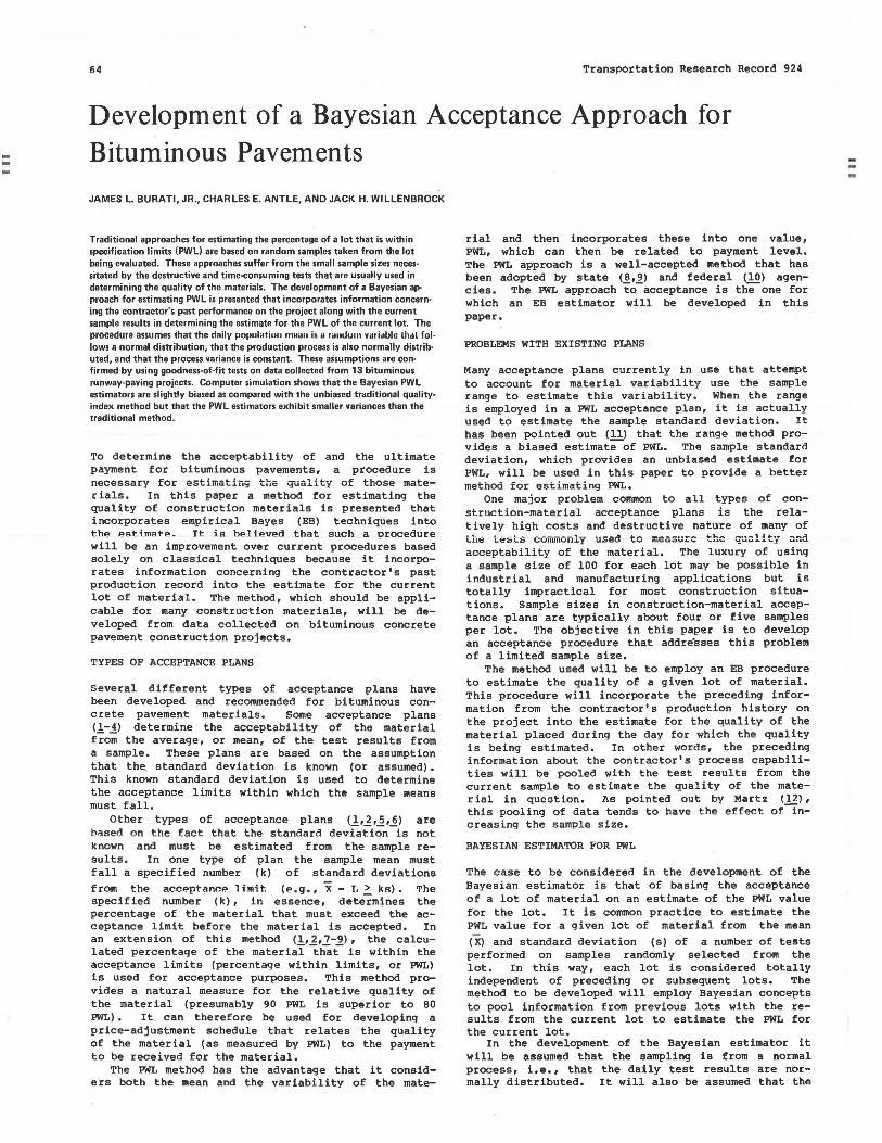
The constant-variance assumption was rejected on 4 of 13 projects for density. Although the con­stant-variance assumption did not fare as well as the two normality assumptions tested by the K-S and CvM procedures, based on the results given in Table 6 it still appears to be a reasonable assumption.

COMPUTER SIMULATION

The performance of the EB estimator for PWL can be evaluated against the traditional method by means of computer simulation. An extensive computer simula-

. ..

70

Table 6. Results of Bartlett test for constant variance on density,

Pooled Test Degrees of Critical Value Project Variance Statistic Freedom (O< = 0 .05) Decision

A 0.8278 18.8862 14 23.68 @ B 2.2600 3.1491 5 11.07 @

c 2.4903 25.3461 18 28.87 @

D 1.3883 11.0024 16 26.30 @ E 0 .333 9.9718 II 19.68 @

F 0.3107 20.3424 9 16.92 x G 0.5200 34.0504 22 33.92 x H 0.7799 6.3637 9 16.92 @

I 0.1255 34.3288 12 21.03 x J 0.5570 13.3109 8 IS.SI @

K l.4526 37.9786 20 31.41 x L 0.5676 19.9066 25 37.64 @

M 0.4250 12.2958 17 27.59 @

Note: @ = do not reject normality assumption; X =reject normality assumption.

tion analysis was conducted with the five methods for estimating PWL that were described previously. A detailed description and discuss i on of this simu­lation analysis hav~ hPPn made (13), and a paper de­tailing this analysis is also currently in prepara­tion. A brief description of the basic simulation procedure used is presented in this paper along with some of the results of the analysis.

Simulation Design

Each simulation run consisted of 3,000 project days. Because paving projects are typically of relatively short duration, the 3,000 project days were made up of 100 projects of 30 days' duration each. In the simulation the values for the daily population means (µi) were generated from a

2

(µp• op) normal distribution. Values of o 2 were

held cons tant for a given project but allowed to vary among projects. For each simulation, however, the ratio of the variance of the daily sample means

2 (0

2 /n) to the preceding variance (op) was held con-

stant for all projects. The ratio [(o 2 /n)/o;J was

chosen to be 2.0, 1.0, or 0.5. A value of 2.0 would favor the EB estimator because it meant that the preceding distribution had a smaller variance than did the daily sample means. Similarly, a value of 0. 5 for this ratio favored the traditional method for estimating PWL because it meant that the preced­ing dis~ribution was more variable than were the daily sample means.

In each simulation conducted, three approaches, designated approaches A, B, and c, were used to es­tablish the initial estimate for the preceding dis­tribution to be used. The approache s were

1. The use of 20 earlier production days to es­tablish a preceding production history for the con­tractor;

2. The use of the first five project production days to establish the precedent for the project in

question; in this app roach , Xi and si were used to estimate PWL in t he traditional manner for the first five project days, and then the EB PWL estimators were used for days 6 through 30; and

3. No knowledge concerning the contractor's pre-

ceding production was assumed; Xi and Bi were used on project days 1 and 2, and then EB PWL estimators were used.

Evaluation Procedure

A number of different measures for evaluating the performance of the EB PWL estimators (methods 2-5)

Transportation Research Record 924

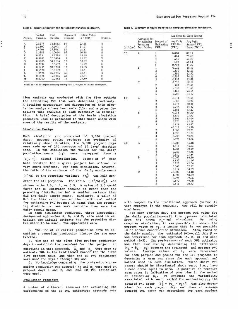
Table 7. Summary of results from typical computer simulation for density.

(a2 /n)/a~

Approach for Establishing Preceding Distribution

0.5 A

B

c

1.0 A

B

c

2.0 A

B

c

Method of Estimating PWL

I 2 3 4 s I 2 3 4 s I 2 3 4 5

I 2 3 4 s I 2 3 4 5 I 2 3 4 5

l 2 3 4 s I 2 3 4 s I 2 3 4,

5

Avg Error for Each Project

Avg Daily PWL Error (PWL)

0.020 1.814 1.645 1.094 0.792 0.020 1.550 1.396 0.997 0.737 0.020 1.787 i .633 1.169 0.900

--0.011 1.688 1.374 0.944 0.581

-0.011 1.357 1.106 0.770 0.454

-0.011 1.585 1.323 0.928 0.596

-0.007 1.511 1.086 0.789 0.380

-0.007 1.135 0.827 0.548 0.214

-0.007 1.321 0.998 0.670 0.313

Avg Daily Squared PWL enor (PWL 2 )

88.19 76.45 52.30 66.51 44.20 88.19 82.21 62.30 74.86 55.68 88.19 82.69 6i .60 74.56 54.12

85.50 64.20 40.88 54.42 33.22 85.50 73.92 53.04 65.16 45.67 85.50 72.79 51.02 63.23 42.86

84.40 54.93 30.59 44.88 23.54 84.40 61.16 42.06 52.92 34.59 84.40 58.72 39.06 49.70 30.73

with respect to the traditional approach (method 1) were employed in the ana lysis. Two will be consid­ered here.

For each project day, the correct PWL value for the daily population--call this p i--was calculated from the known µC and a 2 -values . By us i ng computer simulation, it was possible to obtain the correct value of Pi• a l UlC Ury that is not possible in an actual construction situation . Also, based on the daily sample, the estimated PWL--call this Pi-­was determined for each approach (A, B, C) and each method (1-5). The perform~nr.P of P.ach PWL estimator was then evaluated by dete r min i ng the differenc e ( 6 i =Pi - Pi) between t he estimated and correct PWL values. Average values of o i were determined for each project and pooled for the 100 projects to determi ne a mean PWL error for each approach and method used in each simulation, These daily PWL errors should be distr i buted about zero, i.e., have a mean error equal to zero. A positive or negative mean error is indicative of some bias in the method of estimating Pi• To evaluate the variabil i t y assoc i ated wi th each method for estimating Pir the

squared PWL error [6~ • <Pi - Pil 2 l was also deter­mined for each project day, and then an average squared PWL error was determined for each proj ect

-

Transportation Research Record 924

and for the entire simulation for each method of estimating Pi.

Analysis of Results

The results of a typical computer simulation for density are given in Table 7 (n = 4). In this table, method l is the traditional quality-index ap-proach (based on Xi and sil and can be used as the control against which to measure the performance of the EB PWL estimators.

A review of Table 7 indicates that the tradi­tional estimator produces a better estimate in terms of the average PWL error (6) because the average error is nearly zero; i.e., it is an unbiased esti­mator. The EB estimators, on the other hand, pro­duce average errors that are slightly biased toward the high side. Nevertheless, the EB estimators al­ways produce a lower average squared error than the traditional method. This means that the EB estimate for PWL has a higher likelihood of being close to the true PWL value because it has less variability associated with it. Space does not allow a detailed analysis of the results in Table 7 here. A thorough discussion of the results of the computer simulation analyses may be found elsewhere (13).

CONCLUSIONS

In this paper the steps involved in the development of an acceptance approach for bituminous pavements based on EB techniques are presented. The approach developed uses a Bayesian estimator for the percent­age of the lot of material within specification lim­its (PWL) for determining the level of quality for the pavement. The estimator was developed on the basis of three assumptions:

1. The production process follows a normal dis­tribution,

2. The daily population means follow a normal distribution, and

3. There is a constant process variance.

GOF tests conducted on data collected from 13 bitu­minous runway-paving projects verified the reason­ableness of the three assumptions. Computer simula­tion indicated that the Bayesian estimators for PWL were slightly biased toward higher estimated PWL values but that they had a lower variance for the estimated PWL value than that obtained with the tra­ditional quality-index method.

REFERENCES

1. F.J. Bowery and S.B . Hudson. Statistically Oriented End-Result Specifications. NCHRP, Synthesis of Highway Practice 38, 1976.

2. Quality Assurance and Acceptance Procedures. HRB, Special Rept. 118, 1971.

3. v. Adam. Louisiana Experience with End-Result Specifications for Construction of Asphaltic Concrete. National Asphalt Pavement Associa­tion, Paving Forum, Fall-Winter 1972.

71

4. A.W. Manton-Hall. Comparison of Operating Characteristics of Overlapping and Non-Overlap­ping "Means of n" Type Specifications. Univ. of New South Wales, Sydney, Australia, UNICIV Rept. R-171, Aug. 1977.

s. B.A. Brakey. Statistical Acceptance as In­cluded in the Colorado Sampling and Testing Program. Presented at FHWA Quality Assurance Conference, Albuquerque, N. Mex., May 1976.

6. R.B. Delbert. Application of End-Result Speci­fications to the Production and Laydown of Bi­tuminous Mixtures. Presented at Annual Meet­ing, AAPT, Cleveland, Ohio, Feb. 1972.

7. Improved Quality Assurance of Bituminous Pave­ments. FHWA, 1973.

8. R.M. weed. Optimum Performance Under a Statis­tical Specification. Presented at the 58th An­nual Meeting, TRB, 1979.

9. J.H. Willenbrock and P.A. Kopac. A Methodology for the Development of Price Adjustment Systems for Statistically Based Restricted Performance Specifications. Pennsylvania Transportation Institute, Pennsylvania State Univ., University Park, Rept. FHWA-PA-74-27(1), Oct. 1976.

10. Item P-401: Bituminous Surface Course. East­ern Region, Federal Aviation Administration, June 1982.

11. J.H. Willenbrock and P.A. Kopac. The Develop­ment of Tables for Estimating Percentage of Ma­terial within Specification Limits. Pennsyl­vania Transportation Institute, Pennsylvania State Univ., University Park, Rept. FHWA-PA-74-27(2), Oct. 1976.

12. H.F. Martz. Empirical Bayes Estimation in Quality Control and Reliability: An Exposition and Illustration. Presented at 1974 Annual Meeting of the American Statistical Associa­tion, St. Louis, Mo., Aug. 1974.

13. J.L. Burati. Development of a Bayesian Accept­ance Plan for Bituminous Pavements. Pennsyl­vania State Univ., University Park, Ph.D. thesis, 1982.

14. D.T. Phillips. Applied Goodness of Fit Test­ing. American Institute of Industrial Engi­neers, Norcross, Ga., OR Monograph Series No. 1, 1972.

15. H.W. Lilliefors. On the Kolmogorov-Smirnov Test for Normality with Mean and Variance Un­known. Journal of the American Statistical Association, June 1967, pp. 399-402.

16. R.F. Walpole and R.H. Meyers. Probability and Statistics for Engineers and Scientists. Mac­millan, New York, 1972.

17. J. Neter and w. Wasserman. Applied Linear Sta­tistical Methods. Richard D. Irwin, Inc., Homewood, Ill., 1974,

Publication of this paper sponsored by Committ~e on Quality Assurance and Acceptance Procedures.