Embed Size (px)
Citation preview

DEVELOPMENT AND VALIDATION OF A COMPUTATIONAL MULTIBODY
MODEL OF THE ELBOW JOINT
A THESIS IN
Mechanical Engineering
Presented to the Faculty of the University
of Missouri-Kansas City in partial fulfillment of
the requirements for the degree
MASTER OF SCIENCE
by
MD MUNSUR RAHMAN
B.S., Bangladesh University of Engineering and Technology, 2009
Kansas City, Missouri
2013

© 2013
MD MUNSUR RAHMAN
ALL RIGHTS RESERVED
iii
DEVELOPMENT AND VALIDATION OF A COMPUTATIONAL MULTIBODY
MODEL OF THE ELBOW JOINT
MD MUNSUR RAHMAN, Candidate for the Master of Science Degree
University of Missouri – Kansas City, 2013
ABSTRACT
Computational multibody models of the elbow joint can provide a powerful tool to
study joint biomechanics, examine muscle and ligament function, soft tissue loading, and the
effects of joint trauma. Such models can reduce the cost of expensive experimental testing
and can predict some parameters that are difficult to investigate experimentally, such as
forces within ligaments and contact forces between cartilage covered bones. These
parameters can assist surgeons and other investigators to develop better treatments for elbow
injuries and thereby increase patient care. Biomechanical computational models of the elbow
exist in the literature, but these models are typically limited in their applicability by
artificially constraining the joint (e.g. modeling the elbow as a hinge joint), prescribing
specific kinematics, simplifying ligament characteristics or ignoring cartilage geometries.
The purpose of this thesis was to develop anatomically correct subject specific computational
multibody models of elbow joints and validate these models against experimental data. In
these models, the joints were constrained by three-dimensional deformable contacts between
articulating geometries, passive muscle loading, and multiple bundles of non-linear ligaments
wrapped around the bones.

iv
In this approach, three-dimensional bone geometries for the model were constructed
from volume images generated by computed tomography (CT) scans obtained from cadaver
elbows. The ligaments and triceps tendon were modeled as spring-damper elements with
non-linear stiffness. Articular cartilage was represented as uniform thickness solids covering
the articulating bone surfaces. Finally, the model was validated by placing the cadaver
elbows in a mechanical testing apparatus and comparing predicted kinematics and triceps
tendon forces to experimentally measured values. A small improvement in predicted
kinematics was observed compared to experimental values when the lateral ulnar collateral
and annular ligament were wrapped around the bone. Some reductions of RMS error were
also observed when a non-linear toe region was modeled in the ligament compared to models
that had only a linear force-displacement relationship. None of these changes were
statistically significant (ANOVA p-value was greater than 0.05).

v
The undersigned, appointed by the Dean of School of Computing and Engineering,
have examined the thesis titled " Development and Validation of a Computational Multibody
Model of the Elbow Joint," presented by Md Munsur Rahman, candidate for the Master of
Science in Mechanical Engineering degree, and thereby certify that in their opinion it is
worthy of acceptance.
Supervisory Committee
Trent M. Guess, Ph.D
Associate Professor
School of Computing and Engineering
Ganesh Thiagarajan, Ph.D
Associate Professor
School of Computing and Engineering
Gregory W. King, Ph.D
Assistant Professor
School of Computing and Engineering
vi
TABLE OF CONTENTS
ABSTRACT ................................................................................................................. iii
LIST OF ILLUSTRATIONS ..................................................................................... viii
LIST OF TABLES ....................................................................................................... xi
ACKNOWLEDGMENTS .......................................................................................... xii
Chapter
1. INTRODUCTION ............................................................................................... 13
2. BACKGROUND ................................................................................................. 18
2.1 Elbow anatomy .............................................................................................. 18
2.1.1 Bone anatomy ................................................................................. 19
2.1.2 Ligament anatomy .......................................................................... 22
2.1.3 Muscle anatomy .............................................................................. 25
2.1.4 Joint kinematics .............................................................................. 27
3. METHODS AND MATERIALS ........................................................................ 30
3.1 Cadaver elbow measurements and testing ................................................ 30
3.2 Multibody model formulations ................................................................. 36
4. RESULT .............................................................................................................. 50
4.1 RMS error ................................................................................................. 51
4.2 Ulna kinematics ........................................................................................ 52
4.3 Radius kinematics ..................................................................................... 56
vii
4.3 Triceps tendon forces ................................................................................ 60
5. DISCUSSION ..................................................................................................... 62
5.1 Study limitations ....................................................................................... 64
5.2 Future work ............................................................................................... 65
5.3 Conclusion ................................................................................................ 66
Appendix
A. KINEMATICS COMPARISON FOR SPECIMEN 2 AND 3 ........................... 67
REFERENCES ........................................................................................................... 71
VITA ........................................................................................................................... 79

viii
LIST OF ILLUSTRATIONS
Figure Page
2.1. (A) The view of entire upper extremity and (B) the articulations of
elbow joint. Source: Ferreira (2011). ......................................................... 18
2.2. Osteology of the elbow joint. Anterior (left) and a posterior (right)
view of the right elbow is shown. Source: Netter and
Hansen (2003). ........................................................................................... 19
2.3. Osteology of ulna and radius. Anterior (left) and lateral view of
ulna (right). Source: Tate (2012) ................................................................ 22
2.4. Medial (left) and Lateral (right) collateral ligament complex.
Source: Morrey (2000). .............................................................................. 23
2.5. Interosseous membrane of the forearm. Source: Fisk (2007). ............................... 25
2.6. View of the four major muscles crossing the elbow joint. Source:
("Identify the muscles crossing the elbow joint," 2013) ............................ 27
2.7. (A) The flexion-extension and (B) pronation supination view of
forearm. Right arm is shown. Source: Ferreira (2011). ............................. 29
3.1. (a) The disarticulated radius for specimen 1. The radius was cut
from the distal radioulnar joint and the ulna was cemented
directly to the cup. (b) A ten hole steel dynamic
compression plate was used to constrain the ulna for
specimens 2 and 3. ..................................................................................... 32
3.2. Triceps tendon attachment to the load cell and motion applied by
the mechanical tester. ................................................................................. 33
3.3. Laxity test to measure the zero load length. ........................................................... 34
3.4. Auto threshold segmentation of CT images to isolate the bone
geometries in 3D Slicer. ............................................................................. 37
3.5. Three-dimensional bone geometries a) before and b) after post
processing in Geomagic Studio. ................................................................. 38
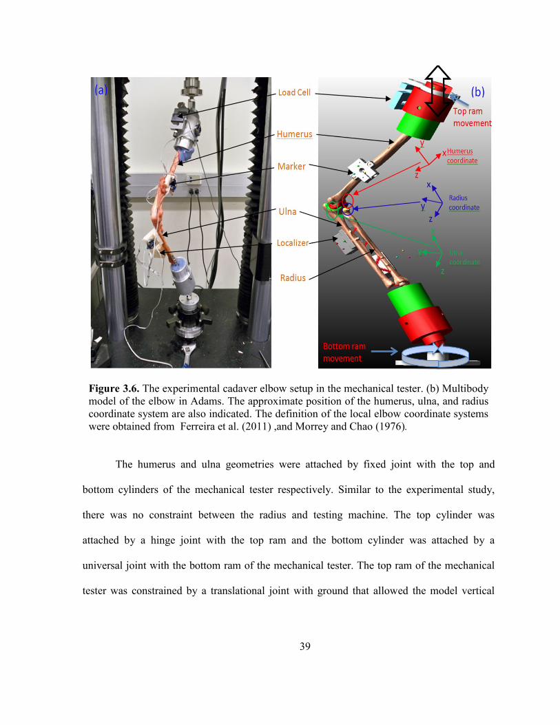
3.6. The experimental cadaver elbow setup in the mechanical tester. (b)
Multibody model of the elbow in Adams. The approximate
position of the humerus, ulna, and radius coordinate system
are also indicated. The definition of the local elbow
coordinate systems were obtained from Ferreira et al.
(2011) ,and Morrey and Chao (1976). ....................................................... 39
3.7. The force-displacement relationship for the central bundle of the
medial collateral ligament (cMCL) anterior part. The

ix
measured zero-load length of the cMCL was 17.2 mm and
the stiffness coefficient in the linear region was 24.1 N/mm. .................... 41
3.8. Interosseous membrane and distal radioulnar ligaments in the
model. Right limb shown. .......................................................................... 43
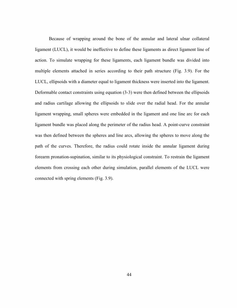
3.9. Wrapping of the LUCL and annular ligament around the bone. Also
shown is the point-curve constraints and parallel connection
between two spheres of the LUCL and annular ligaments. ....................... 45
3.10. Approximate position and orientation of the elbow joint coordinate
system. Source: Ferreira (2011). ................................................................ 47
4.1. Superior-inferior (S-I) displacement of the ulna coordinate system
relative to the humerus coordinates for specimen 1. .................................. 52
4.2. Anterior-posterior (A-P) displacement of the ulna coordinate
system relative to the humerus coordinates for specimen 1. ...................... 53
4.3. Medial-lateral (M-L) displacement of the ulna coordinate system
relative to the humerus coordinates for specimen 1. .................................. 53
4.4. Ulna internal-external (I-E) rotation relative to the humerus
coordinates for specimen 1......................................................................... 54
4.5. Ulna adduction-abduction (AD-AB duction) relative to the humerus
coordinates for specimen 1......................................................................... 55
4.6. Ulna flexion-extension (F-E) relative to the humerus coordinates for
specimen 1. ................................................................................................. 55
4.7. S-I displacement of the radius coordinate system relative to the
humerus coordinates for specimen 1. ......................................................... 56
4.8. A-P displacement of the radius coordinate system relative to the
humerus coordinates for specimen 1. ......................................................... 57
4.9. M-L displacement of the radius coordinate system relative to the
humerus coordinates for specimen 1. ......................................................... 57
4.10. Radius I-E rotation relative to the humerus coordinates for
specimen 1. ................................................................................................. 58
4.11. Radius I-E rotation relative to the humerus coordinates for
specimen 1 .................................................................................................. 59
4.12. Radius AD-AB duction relative to the humerus coordinates for
specimen 1. ................................................................................................. 59
4.13. Comparison of triceps tendon force for specimen 1............................................. 60
A.1. Measured and predicted displacement and rotation of the ulna
coordinate system relative to the humerus coordinate system
for specimen 2. ........................................................................................... 67

x
A.2 Measured and predicted displacement and rotation of the radius
coordinate system relative to the humerus coordinate system
for specimen 2. ........................................................................................... 68
A.3. Measured and predicted displacement and rotation of the ulna
coordinate system relative to the humerus coordinate system
for specimen 3. ........................................................................................... 69
A.4. Measured and predicted displacement and rotation of the radius
coordinate system relative to the humerus coordinate system
for specimen 3. ........................................................................................... 70
xi
LIST OF TABLES
Table Page
3.1. Information regarding each cadaver elbow used in this study. .............................. 31
3.2. Elbow flexion angle during movement. ................................................................. 35
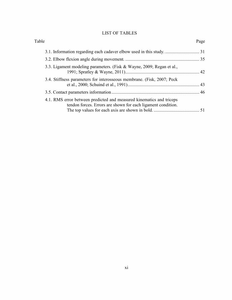
3.3. Ligament modeling parameters. (Fisk & Wayne, 2009; Regan et al.,
1991; Spratley & Wayne, 2011)................................................................. 42
3.4. Stiffness parameters for interosseous membrane. (Fisk, 2007; Peck
et al., 2000; Schuind et al., 1991) ............................................................... 43
3.5. Contact parameters information ............................................................................. 46
4.1. RMS error between predicted and measured kinematics and triceps
tendon forces. Errors are shown for each ligament condition.
The top values for each axis are shown in bold. ........................................ 51

xii
ACKNOWLEDGMENTS
I would like to thank the School of Medicine, University of Missouri-Kansas City
(UMKC), for funding this research.
I would like to acknowledge many people who have helped and provided support for
me during this project. To begin with my advisor Dr. Guess, who has provided a great
opportunity to work in the Musculoskeletal Biomechanics Research Laboratory and enabled
me to have a fulfilling research experience. He opened the door to a subject that I have
become passionate about. His guidance, support, and wisdom have also been indispensable. I
would also like to acknowledge Dr. Akin Cil for his support and guidance to successfully finish
this research. I would like to thank my advisory committee members Dr. Thiagarajan and Dr.
King for taking the time and effort to serve on my committee. I want to thank my lab partners
Mohammad Kia, Antonis Stylianou, and Katherine Bloemker, Yunkai Lu for helping
troubleshoot problems.
I would also like to thank my wife Mashruba for her unwavering support and care
throughout this process.

13
CHAPTER 1
INTRODUCTION
The human elbow joint is a unique joint that produces the complex motion of the
forearm for hand positioning and allows humans to accomplish numerous significant
activities in their daily life that makes them distinct from other mammals (Gonzalez,
Hutchins, Barr, & Abraham, 1996).Unfortunately, this most important joint of the upper
extremity (Morrey, 2000) has been recognized as the second most commonly dislocated joint
in adults (de Haan et al., 2011). Although not as common as in the knee joint, osteoarthritis
of the elbow can cause severe pain in the joint, loss of joint mobility, and can be a cause of
entire upper limb disability (Degreef & De Smet, 2011). The enervating nature of
osteoarthritis is well established, but the underlying reasons of this chronic disease are not
completely understood. Furthermore, fracture, tennis elbow, tendinitis, bursitis, and motion
impingement can be significantly debilitating for the elbow joint. Additionally, the high
frequency of dislocation (Wiesel & Delahay, 2010), complexity of posttraumatic instability
(Ring & Jupiter, 2000), and operative complications associate with joint trauma (Ring &
Jupiter, 2000) have made the elbow joint an important focus of research (Fisk, 2007).
Detailed knowledge of the in vivo loading of elbow structures is important to
understand the biomechanical causes associated with joint degeneration and injuries and to
find suitable treatment. Prediction of joint and tissue level loading during elbow activities has
a great potential to significantly improve orthopaedic repair. In addition, better
understanding of in vivo mechanical loads has good indications regarding the development
14
and progression of osteoarthritis and thereby reduces the cost of treatment (Guess,
Thiagarajan, Kia, & Mishra, 2010). Likewise, knowledge of in vivo ligament and tendon
forces of elbow joint would provide valuable insight regarding joint stability and injury
mechanism. But currently, measuring the in vivo tendon and ligament forces and cartilage
contact pressures of the elbow joint during various activities is not possible.
Computational multibody models can be a potential tool to predict tendon, ligament
and contact forces (Cohen, Henry, McCarthy, Mow, & Ateshian, 2003; Giddings, Beaupre,
Whalen, & Carter, 2000; Hirokawa, 1991; Kwak, Blankevoort, & Ateshian, 2000; Lemay &
Crago, 1996; Shelburne, Pandy, Anderson, & Torry, 2004; Wismans, Veldpaus, Janssen,
Huson, & Struben, 1980). These models could provide valuable understanding to the in vivo
loading environment of the elbow joint and enhance our comprehension of elbow mechanics
and tissue interactions during dynamic activities (Guess, 2012). Therefore, computational
multibody models of the elbow could be a valuable tool to improve the diagnosis, treatment
and rehabilitation of post-traumatic injuries of the elbow joint. Many researchers have used
these model to investigate muscle contribution to joint moment (Arnold & Delp, 2001;
Gonzalez et al., 1996; Hutchins, Gonzalez, & Barr, 1993; Lemay & Crago, 1996; Murray,
Delp, & Buchanan, 1995; van der Helm, 1994a) and body segment motion (Anderson &
Pandy, 2001; Gonzalez, Abraham, Barr, & Buchanan, 1999; Nagano, Komura, Yoshioka, &
Fukashiro, 2005; Peck, Langenbach, & Hannam, 2000; van der Helm, 1994b). A validated
model can be used as a potential biomechanical tool for patient-specific preoperative
planning, computer-aided surgery, and computer-aided rehabilitation (Chao, Armiger,
Yoshida, Lim, & Haraguchi, 2007; Fernandez & Pandy, 2006; Fisk & Wayne, 2009;

15
Holzbaur, Murray, & Delp, 2005; Kwak et al., 2000; Woo, Debski, Wong, Yagi, & Tarinelli,
1999).
Two main tools have been used in biomechanics for developing computational
models: finite element analysis (FEA) (Giddings et al., 2000; Li, Gil, Kanamori, & Woo,
1999; van der Helm, 1994b; Wu, Dong, Smutz, & Schopper, 2003) and multibody dynamics
(MBD) (Anderson & Pandy, 2001; Barker, Kirtley, & Ratanapinunchai, 1997; Chaudhari &
Andriacchi, 2006; Cohen et al., 2003; Freund & Takala, 2001; Gonzalez, Andritsos, Barr, &
Abraham, 1993; Gonzalez et al., 1996; Hirokawa, 1991; Iwasaki et al., 1998; Kwak et al.,
2000; Lemay & Crago, 1996; Li et al., 1999; Liacouras & Wayne, 2007; Lin et al., 2005;
Morey-Klapsing, Arampatzis, & Bruggemann, 2005; Nagano et al., 2005; Peck et al., 2000;
Piazza & Delp, 2001; Raikova, 1992, 1996; Shelburne et al., 2004; Triolo, Werner, & Kirsch,
2001; Wismans et al., 1980). FEA has the ability to predict the stress and strain within tissue
in articulating contacts. The models are based on the concepts of continuum mechanics and
contain many equations and unknown variables. As a result, finite element models take
extensive amounts of time for both development and simulation. Therefore, FEA is not an
efficient option in body level dynamic simulation (Guess & Stylianou, 2012). On the other
hand, multibody modeling uses rigid body dynamics algorithms where the models have
fewer unknown variables. MBD simulations are computationally efficient for dynamic
simulation compared to FEA. As a result, for the situations where calculating bone
deformation or stress-strain computations are not the choice, multibody modeling could be an
appealing option. Many researchers have applied multibody models for specific applications
such as predicting joint stability, joint contact areas and pressure, ligament functions, muscle
contributions to joint moments, body segment motion, and menisci effect in the knee
16
(Donahue, Hull, Rashid, & Jacobs, 2002; Ferreira, King, & Johnson, 2011; Fisk & Wayne,
2009; Guess, 2012; Guess, Liu, Bhashyam, & Thiagarajan, 2013; Guess et al., 2010;
Stylianou, Guess, & Cook, 2012; Zielinska & Donahue, 2006).
Numerous studies of computational modeling have been developed to investigate
joint behavior (Buchanan, Delp, & Solbeck, 1998; Fisk & Wayne, 2009; Garner & Pandy,
2001; Gonzalez et al., 1999; Gonzalez et al., 1996; Holzbaur et al., 2005; Kwak et al., 2000;
Lemay & Crago, 1996; Raikova, 1992; Schuind et al., 1991; Spratley & Wayne, 2011; Triolo
et al., 2001). Gonzalez et al. (1996) developed a computational elbow model to investigate
the elbow joint movement, relationship among muscle excitation patterns, and to determine
the effects of forearm and elbow position on the recruitment of individual muscles during
ballistic movements. Holzbaur et al. (2005) developed a three-dimensional model of the
upper extremity that comprises all the major muscles of the upper limb and provides accurate
estimation of muscle moment arms. Lemay and Crago (1996) developed a dynamic skeletal
model of the elbow joint where the model movements were produced by activation of Hill-
type muscle models and were capable of simulating elbow and wrist flexion-extension, and
radial-ulnar deviation movement. However, these models have assumed the joint structure to
have idealized joint motion (e.g. hinge joint) rather than true anatomical joint motion
constrained by ligament force and cartilage contact. Although in some circumstance such
simplification would be helpful for our understanding of joint kinematics and muscle
functions, it is not always appropriate to assume a human joint as a generalized mechanical
joint (Benham, Wright, & Bibb, 2001). These presumptions decrease the validity of model
results, and prevent investigation of ligament function and joint laxity (Fisk, 2007). Fewer
biomechanical models of the elbow joint have investigated the ligamentous constraints,

17
articular surface contact, and muscle loading effect on joint stability, but have not included
wrapping of ligaments around bone, the non-linear ligament ‘toe’ region, and articular
cartilage contribution (Fisk & Wayne, 2009; Spratley & Wayne, 2011). Irrespective of any
modeling assumption, some models have been limited by model validation (Chao et al.,
2007; Delp & Loan, 1995; Fernandez & Pandy, 2006; Kwak et al., 2000; Woo et al., 1999).
Model predicted results should be compared with experimental data before a computational
model can be used as a predictive and meaningful tool (Fisk, 2007).
The main purpose of this thesis is to develop an anatomically correct computational
elbow joint model that includes representation of articular cartilage. The elbow joint is
constrained by three-dimensional contact between articular bone geometries, triceps tendon
loading, and multiple ligament bundles having a non-linear toe region. Wrapping of the
lateral ulnar collateral and annular ligaments around the bone are also considered. This study
has examined the effects of articular contacts and different ligament loading on kinematics
during elbow flexion-extension associated with forearm pronation-supination. The models
have used easily accessible, well documented commercial software for developing the
computational models. The models are validated by comparing the predicted humerus,
radius, ulna kinematics and passive triceps tendon forces to identically loaded experimentally
measured values. Developing anatomically correct elbow models in the multibody
framework for incorporation in musculoskeletal models of the upper extremities is the overall
goal of this research.

18
CHAPTER 2
BACKGROUND
2.1 Elbow anatomy
Elbows play an important role for positioning and orientating the upper arm in three-
dimensional space. Careful examination of elbow anatomy is important to understand the
significant influences of various components on joint structure and behavior. Anatomy of the
elbow is relevant to all structures that accomplish and affect elbow motion such as bone,
ligaments, and muscle. As the most important joint of the upper extremity (Alcid, Ahmad, &
Lee, 2004), the elbow joint is comprised of all three long bones of the arm; humerus, radius,
and ulna (Fig. 2.1).
Figure 2.1. (A) The view of entire upper extremity and (B) the articulations of elbow joint.
Source: Ferreira (2011).
19
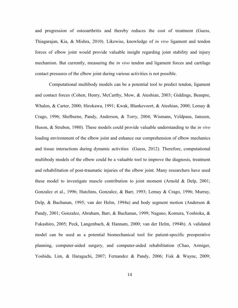
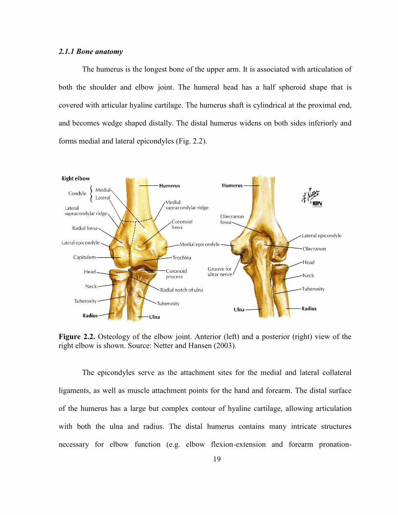
2.1.1 Bone anatomy
The humerus is the longest bone of the upper arm. It is associated with articulation of
both the shoulder and elbow joint. The humeral head has a half spheroid shape that is
covered with articular hyaline cartilage. The humerus shaft is cylindrical at the proximal end,
and becomes wedge shaped distally. The distal humerus widens on both sides inferiorly and
forms medial and lateral epicondyles (Fig. 2.2).
Figure 2.2. Osteology of the elbow joint. Anterior (left) and a posterior (right) view of the
right elbow is shown. Source: Netter and Hansen (2003).
The epicondyles serve as the attachment sites for the medial and lateral collateral
ligaments, as well as muscle attachment points for the hand and forearm. The distal surface
of the humerus has a large but complex contour of hyaline cartilage, allowing articulation
with both the ulna and radius. The distal humerus contains many intricate structures
necessary for elbow function (e.g. elbow flexion-extension and forearm pronation-

20
supination). Adjacent to the medial epicondyle is the spool-shaped surface of the trochlea.
The trochlea surface is covered by 3000 of articular cartilage (Chuang, Wu, Lin, & Lur, 2012;
Morrey, 2000) which articulates with the greater sigmoid notch of the ulna. This surface has
a circular cross-section in the sagittal plane and contains the trochlear sulcus at the center
which provides an articular bearing surface for flexion-extension motion. The trochlear
sulcus with the medial and lateral lips forms a track that keeps the greater sigmoid notch of
the ulna centered. Lateral to the trochlea is the capitulum that has a nearly spherical structure.
The capitulum is covered with articular cartilage by approximately 1800 (Ferreira, 2011) that
allows articulation with the concave dish of the radial head and provides a bearing for both
elbow flexion-extension and forearm pronation-supination. Two groove structures located
superior to trochlear and capitulum are called the coronoid fossa and radial fossa respectively
(Fig. 2.2). The depression region on the posterior distal humerus is the olecranon fossa that
provides clearance of the ulna’s olecranon at high elbow extension.
Structures of the proximal radius include several crucial features that are necessary
for proper elbow operation. At its most proximal aspect is the cup-shaped structure called the
radial head (Fig. 2.2). The axis of the radial head and the adjacent neck make a 150 angle
with the radius shaft (Morrey, 2000). The radial head is fully enveloped with articular
cartilage and provides articulation with the capitulum to allow forearm rotation. The
circumference of the radial head is also covered with hyaline cartilage by 2400 (Ferreira,
2011). This cartilage contributes to articulation with the lesser sigmoid notch of the proximal
ulna and forms the proximal radioulnar joint. A bony outcropping at the distal radius is the
radial tubercle that serves as the insertion site for biceps tendon (Morrey, 2000).

21
The proximal ulna has some very significant structures for elbow function. Most
superiorly, the ulna bone comes forward, approximating the form of a beak (Fig. 2.2). This
beak is called the olecranon process. The anteriorly extended surface is called coronoid
process that stays distally from the olecranon process. The olecranon and coronoid process
fits into their corresponding fossae during full elbow flexion and extension. The cartilage
enveloped region of the proximal ulna is divided into two regions; the lesser and greater
sigmoid notch. The lesser sigmoid notch has 60-80° of articular cartilage that articulates
with the radial head and forms the proximal radioulnar joint (PRUJ) which provides forearm
pronation-supination. The greater sigmoid notch generates articulations with the distal
humerus where the guiding ridge fits into the track of the trochlear sulcus of the humerus.
Elbow function is also influenced by skeletal features distal to the joint. The diaphysis
shafts of the ulna and radius area are triangular in cross section and run almost parallel to
each other to the distal end when the forearm is supinated (Fig. 2.3). Interosseous margin
areas are located at the medial and lateral boundaries of the supinated radius and ulna
diaphysis respectively. The radius becomes tapered as it goes distally to its limit, but the ulna
expands with triangular structure till it terminates at its distal head. At the distal end of the
radius, the bony lateral extension is called the styloid process. The styloid process provides
attachments for ligaments of the wrist. At the distal end of the ulna, the cartilage covered
knoblike head articulates laterally with a notch on the radius (ulnar notch) and forms the
distal radioulnar joint. This joint, together with the proximal radioular joint, provides
articulation for forearm rotational motion. A medial styloid process located at the distal end
of the ulna provides attachments for ligaments of the wrist.

22
Figure 2.3. Osteology of ulna and radius. Anterior (left) and lateral view of ulna (right).
Source: Tate (2012)
2.1.2 Ligament anatomy
The bony structures of the elbow joint are restrained and stabilized by other passive
structures. Predominantly, the medial and lateral collateral ligaments are two major
ligamentous structures that contribute to primary stabilization of the elbow. The forearm is
largely stabilized by the interosseous membrane between the ulna and radius. Distal
radioulnar ligaments, located at distal radioulnar joint, can also influence elbow behavior.
23
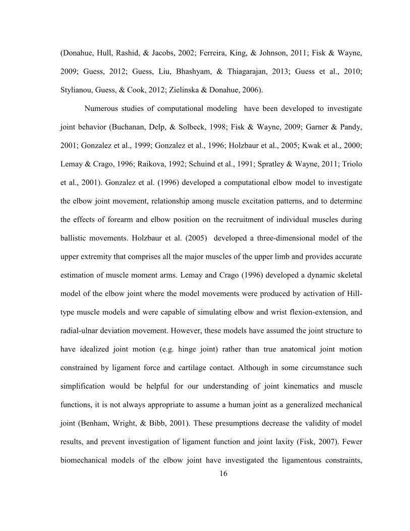
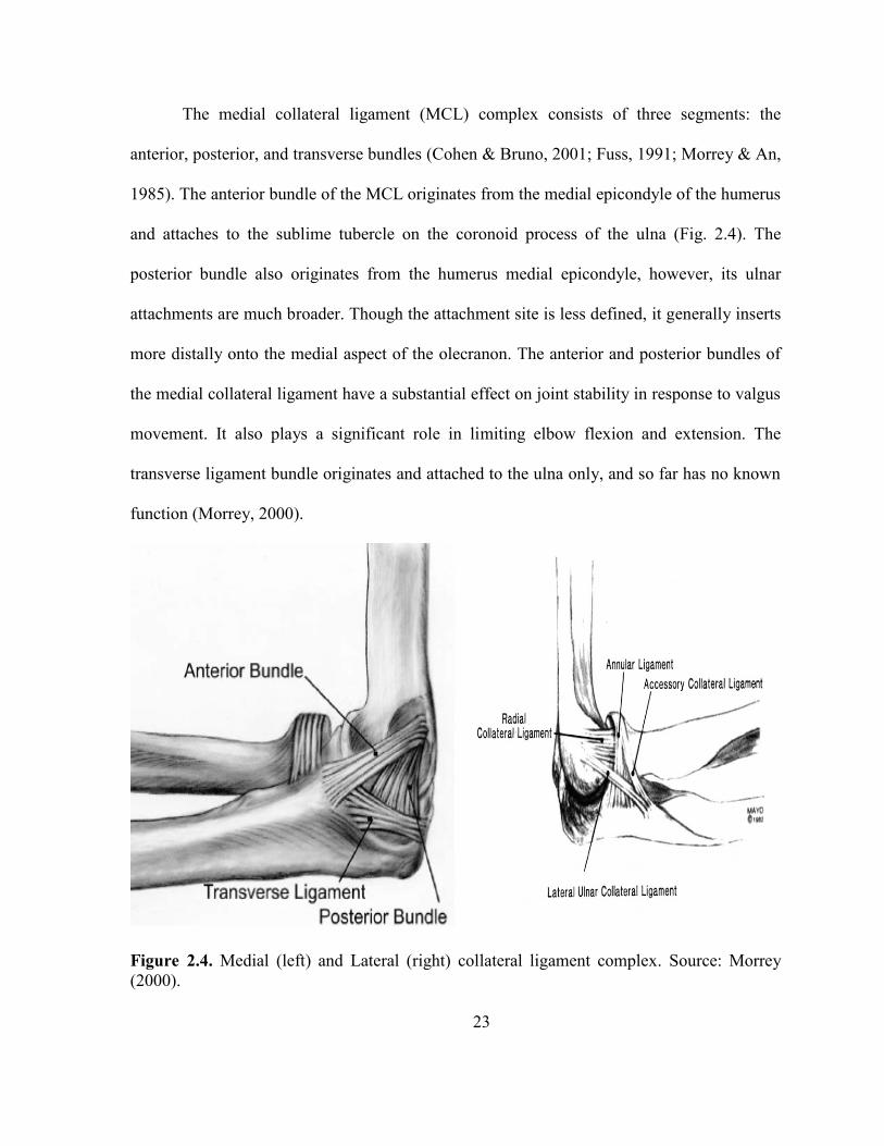
The medial collateral ligament (MCL) complex consists of three segments: the
anterior, posterior, and transverse bundles (Cohen & Bruno, 2001; Fuss, 1991; Morrey & An,
1985). The anterior bundle of the MCL originates from the medial epicondyle of the humerus
and attaches to the sublime tubercle on the coronoid process of the ulna (Fig. 2.4). The
posterior bundle also originates from the humerus medial epicondyle, however, its ulnar
attachments are much broader. Though the attachment site is less defined, it generally inserts
more distally onto the medial aspect of the olecranon. The anterior and posterior bundles of
the medial collateral ligament have a substantial effect on joint stability in response to valgus
movement. It also plays a significant role in limiting elbow flexion and extension. The
transverse ligament bundle originates and attached to the ulna only, and so far has no known
function (Morrey, 2000).
Figure 2.4. Medial (left) and Lateral (right) collateral ligament complex. Source: Morrey
(2000).

24
The lateral collateral ligament (LCL) typically includes four components (Morrey,
2000; Morrey & An, 1985). The lateral ulnar collateral ligament (LUCL) originates from the
lateral epicondyle of the humerus, and inserts in the crista supinatorum tubercle of the ulna
and superficially blends with the annular ligament (Fig. 2.4). The ring-shaped annular
ligament attaches to the anterior rim of the lesser sigmoid notch, wraps around approximately
80% of the radial head and attaches to the posterior rims of the lesser sigmoid notch. The
radial collateral ligament (RCL) originates from the lateral epicondyle of the humerus, fans
out at its distal end, and blends with the lateral portion of the annular ligament. A variable
accessory collateral ligament is sometimes described, which attaches to the crista
supinatorum and blends proximally with the distal lateral rim of the annular ligament
(Morrey, 2000).
Ligaments are viscoelastic (An, 2005), making the ligament mechanical
characteristics dependent on the direction of load and also on loading rate. Each ligament
bundle has fibers orientated in different directions according to the primary tensile force. The
collateral ligaments are heterogeneous structures which are composed of a combination of
collagen and elastin that provide stability of the ligament in various directions. The
interosseous membrane (IOM) is the sturdy thin collagenous sheet that usually attaches on
the interosseous borders of the radius and ulna (Fig. 2.5). It consists of several bands:
proximal band, central band, accessory bands, and distal membranous band (McGinley &
Kozin, 2001; Skahen, Palmer, Werner, & Fortino, 1997). Other than the proximal band, all
interosseous membrane bands runs distally and medially from its radial origin to its ulnar
insertion. The fiber bands make an average 210 angle with the long axis of the ulna (Skahen
et al., 1997). The proximal band is an oblique structure that attaches proximally to the ulna

25
and distally to the radius. The central band shares the insertion with proximal band and is
approximately twice as thick as other bands (Amis, Dowson, & Wright, 1979). Several other
bands are located inferior to the central band; distal to these bands are areas of membranous
tissue. Researchers have suggested that the interosseous membrane also acts as a stabilizer
of the distal radioulnar joint (Schuind et al., 1991).
Figure 2.5. Interosseous membrane of the forearm. Source: Fisk (2007).
2.1.3 Muscle anatomy
Twenty four distinct muscles cross the elbow joint and these muscles originate from
the distal humerus and insert on the forearm and hand (Morrey, 2000; Pigeon, Yahia, &
Feldman, 1996). These muscles produce flexion-extension, forearm pronation-supination,
and flexion-extension of the wrist and fingers. Although all of the muscles are essential for
proper elbow function, only a select subset of muscles that significantly influence elbow
operation will be discussed here.

26
Brachialis, biceps brachii, and brachioradialis are the three muscles that cross the
elbow joint to generate flexion moment (Fig 2.6). The brachialis originates broadly on the
anterior, distal half of the humerus and converges to insert more discretely on the ulnar
tuberosity and base of the coronoid process. The biceps brachaii has two origins (its name is
derived from the Latin word biceps which means “two heads”) and positioned more
superficially on the anterior aspect of the upper arm. The long head originates from the
superior glenoid tubercle of the scapula and wraps around the humeral head and runs down to
the intertubercular sulcus of the humerus. The short head originates from the apex of the
coracoid process of scapula and blends with the long head approximately 7 centimeters
proximal to the elbow to form a single tendon which inserts at the bicipital tuberosity of the
proximal radius. The biceps brachii has a distinct large cross section and insertion on the
medial aspect of the radius, as a result, the biceps works as a powerful forearm supinator.
Particularly, when the forearm is supinated, biceps brachii works as a significant elbow
flexor (Shiba et al., 1988). The brachioradialis originates from the lateral supracondylar ridge
of the humerus and inserts distally at the radial styloid (Morrey, 2000). Brachioradialis has
the longest moment arm of elbow flexion, but due to its small cross section, the
brachioradialis works as the weakest of the three flexor muscles (Hotchkiss, An, Sowa,
Basta, & Weiland, 1989; Murray et al., 1995; Shiba et al., 1988).

27
Figure 2.6. View of the four major muscles crossing the elbow joint. Source:
("Identify the muscles crossing the elbow joint," 2013)
The triceps is the only muscle that generates elbow extension moment. It has three
heads, as its name implies. The long head has the most medial attachment and originates
from the scapula at the infraglenoid tubercle. The lateral head originates on the lateral
intermuscular septum and passes along a thin linear strip superior to the radial groove. The
medial head has a broad origin and attaches to the posteromedial humeral shaft and medial
intermuscular septum. All three heads begin to converge in the middle of the muscle and
ultimately merge to form a single large tendon that inserts at the olecranon process of the
ulna (Morrey, 2000).
2.1.4 Joint kinematics
The ulnohumeral, radiohumeral, proximal radioulnar, and distal radioulnar joint are
described as a trochoginglymoid joint of upper extremities (Morrey, 2000) that jointly

28
construct two distinct forms of motion (flexion-extension and pronation-supination). The
flexion and extension motion is primarily produce by the ulnohumeral joint. The motion axis
for flexion-extension is defined as an axis through the centers of the capitellum and the
trochlear sulcus of the humerus (Currier, 1972). The full flexion range for normal subjects is
approximately from 0° (full extension) to 145° (full flexion) (Figure 2.7A) (Morrey, 2000).
Sometimes the hyperextension obtained from a subject is indicated by a negative flexion
angle. The actual flexion range for an individual can be affected by many reasons such as
prior disease or trauma, the bulk of soft tissue presence, and the ligamentous laxity or
looseness.
Forearm pronation-supination is generated by the incorporation of the radiohumeral,
proximal radioulna, and distal radioulnar articulation. To produce this motion, the ulna
remains stationary and the radius pronates and supinates around it. Rather than circling the
whole radius about the ulna, the distal radius encircles the distal ulna and the proximal radius
pivots about its own center on the capitulum surface. For a normal subject, the attainable
forearm ration range is about 150°-160° (Figure 2.7B) (Morrey, 2000), but it may vary
depending on subject joint condition.
In addition to the above mentioned principal motions, the forearm bones exhibit other
motion patterns. Along with rotation, the radius also moves proximally with pronation and
distally with supination in the sagittal plane (Morrey, 2000). The proximal ulna rotates a few
angles with respect to humerus and pronation-supination also causes the ulna to rotate
internally and externally.

29
Figure 2.7. (A) The flexion-extension and (B) pronation supination view of forearm. Right
arm is shown. Source: Ferreira (2011).
30
CHAPTER 3
METHODS AND MATERIALS
3.1 Cadaver elbow measurements and testing
Three fresh frozen cadaver elbow specimens were used for this study (Table 3.1). The
specimens were thawed at room temperature for 24 hours before collecting medical images.
The elbow donors had never been diagnosed with major elbow diseases and the elbows
appeared normal and intact during visual inspection. Two elbows were imaged with
computed tomography (CT) scans and one was imaged with magnetic resonance imaging
(MRI). The entire arm was scanned to obtain the complete bone lengths. CT scans of the
elbows were taken to create three mutually perpendicular imaging sequences using Syngo CT
(Siemens, Siemens medical solutions, PA) 20108 version software with 8 allocated bits and
fine resolution scan. The parameters used for the CT scan imaging were: slice thickness of
1.5mm, imaging frequency 63.68Hz, spacing between slices 2mm, and group lengths 192.
MRIs were attained using a Siemens 1.5T machine with a narrow field fine resolution setting.
The parameters used for MRI were: TR:13.64, TE:6.82, image resolution 512 x 512, slice
thickness 1.5mm, and spacing between slices 1.875mm. Before imaging, one custom made
ABS plastic “localizer” was rigidly attached with titanium screws to each bone segment
(humerus, ulna and radius) after limited incisions through the skin and soft tissues with the
help of a shoulder and elbow fellowship trained orthopaedic surgeon. During the incisions,
much care was taken to save the joint capsule and ligaments. Every localizer had two
perpendicular tubes that were packed with Vaseline to assist in global coordinate registration
31
later in the experiment (Stylianou et al., 2012). Following medical imaging, the elbows were
dissected by the orthopedic surgeon. Keeping the joint capsule, ligaments, and triceps tendon
intact, all other tissue was removed from the bone.
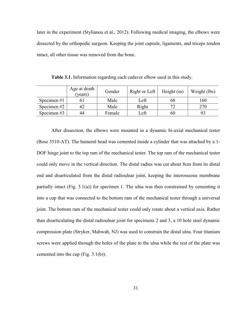
Table 3.1. Information regarding each cadaver elbow used in this study.
Age at death
(years) Gender Right or Left Height (in) Weight (lbs)
Specimen #1 61 Male Left 68 160
Specimen #2 42 Male Right 72 270
Specimen #3 44 Female Left 60 93
After dissection, the elbows were mounted in a dynamic bi-axial mechanical tester
(Bose 3510-AT). The humeral head was cemented inside a cylinder that was attached by a 1-
DOF hinge joint to the top ram of the mechanical tester. The top ram of the mechanical tester
could only move in the vertical direction. The distal radius was cut about 8cm from its distal
end and disarticulated from the distal radioulnar joint, keeping the interosseous membrane
partially intact (Fig. 3.1(a)) for specimen 1. The ulna was then constrained by cementing it
into a cup that was connected to the bottom ram of the mechanical tester through a universal
joint. The bottom ram of the mechanical tester could only rotate about a vertical axis. Rather
than disarticulating the distal radioulnar joint for specimens 2 and 3, a 10 hole steel dynamic
compression plate (Stryker, Mahwah, NJ) was used to constrain the distal ulna. Four titanium
screws were applied through the holes of the plate to the ulna while the rest of the plate was
cemented into the cup (Fig. 3.1(b)).

32
Figure 3.1. (a) The disarticulated radius for specimen 1. The radius was cut from the distal
radioulnar joint and the ulna was cemented directly to the cup. (b) A ten hole steel dynamic
compression plate was used to constrain the ulna for specimens 2 and 3.
The radius had no extra mechanical constraint for all specimens. A 100N load cell
was rigidly attached to the humerus cylinder to measure force in the triceps tendon. The
triceps tendon was threaded with a suture and the suture was attached to the load cell with the
help of a threaded nut and bolt (Fig. 3.2). After attaching the arm to the testing machine,
three rigid-body marker ireds (each containing three infrared markers (Fig. 3.1(a))) were
firmly attached to the humerus, radius, and ulna. The humerus cylinder also had a marker
ired added to it to measure the top ram movement and to aid in computational model
alignment. A 3-camera Optotrak Certus motion Capture system (Northern Digital
Inc,waterloo, Ontario, Canada) was used to track the motion of each bone segment during
experimental testing.

33
Figure 3.2. Triceps tendon attachment to the load cell and motion applied by the mechanical
tester.
Before the experimental trials began, a laxity test was performed to calculate ligament
bundle zero-load lengths (the lengths at which ligament bundles first become taut). To
accomplish the laxity test, the humerus was held in a fixed position (Fig. 3.3) while the ulna
and radius were manually moved through their full range of motion with minimal force
applied (as judged by the experimenter) (Guess et al., 2013). The kinematic envelope of
motion (KEM) was measured from corresponding bone segments by using the attached

34
Optotrak markers and camera system throughout this process. The zero-load length for each
ligament was then determined by calculating the maximum straight-line distance between
insertion and origin sites of the individual ligament throughout the range of motion and then
multiplying by a correction factor. A correction factor of 0.80 was applied to each ligament
bundle (Bloemker, Guess, Maletsky, & Dodd, 2012). The purpose of the correction factor
was to reduce the error inadvertently introduced by the experimenter during the laxity test
when a small amount of force was applied to each ligament when the experimenter moves
the joint throughout its range of motion.
Figure 3.3. Laxity test to measure the zero load length.
Once the laxity test was completed, the arm was put back on the testing machine and
the suture was pulled taut and secured to the load cell. The initial position and orientation of
the cadaveric bone geometries relative to the mechanical tester were determined by recording
multiple points on the localizers, along the bone surfaces, and on the load cell by using a
probing tip of the Optotrak system. The mechanical tester was set at neutral position before
35
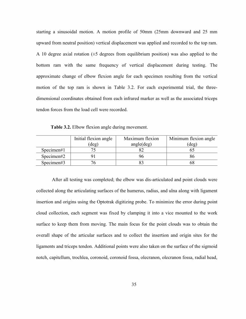
starting a sinusoidal motion. A motion profile of 50mm (25mm downward and 25 mm
upward from neutral position) vertical displacement was applied and recorded to the top ram.
A 10 degree axial rotation (±5 degrees from equilibrium position) was also applied to the
bottom ram with the same frequency of vertical displacement during testing. The
approximate change of elbow flexion angle for each specimen resulting from the vertical
motion of the top ram is shown in Table 3.2. For each experimental trial, the three-
dimensional coordinates obtained from each infrared marker as well as the associated triceps
tendon forces from the load cell were recorded.
Table 3.2. Elbow flexion angle during movement.
Initial flexion angle
(deg)
Maximum flexion
angle(deg)
Minimum flexion angle
(deg)
Specimen#1 75 82 65
Specimen#2 91 96 86
Specimen#3 76 83 68
After all testing was completed; the elbow was dis-articulated and point clouds were
collected along the articulating surfaces of the humerus, radius, and ulna along with ligament
insertion and origins using the Optotrak digitizing probe. To minimize the error during point
cloud collection, each segment was fixed by clamping it into a vice mounted to the work
surface to keep them from moving. The main focus for the point clouds was to obtain the
overall shape of the articular surfaces and to collect the insertion and origin sites for the
ligaments and triceps tendon. Additional points were also taken on the surface of the sigmoid
notch, capitellum, trochlea, coronoid, coronoid fossa, olecranon, olecranon fossa, radial head,
36
radial neck, bicipital tuberosity, and on the diaphyses to aid in orienting the bone geometries
during model generation.
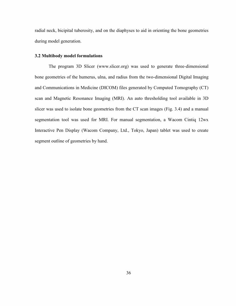
3.2 Multibody model formulations
The program 3D Slicer (www.slicer.org) was used to generate three-dimensional
bone geometries of the humerus, ulna, and radius from the two-dimensional Digital Imaging
and Communications in Medicine (DICOM) files generated by Computed Tomography (CT)
scan and Magnetic Resonance Imaging (MRI). An auto thresholding tool available in 3D
slicer was used to isolate bone geometries from the CT scan images (Fig. 3.4) and a manual
segmentation tool was used for MRI. For manual segmentation, a Wacom Cintiq 12wx
Interactive Pen Display (Wacom Company, Ltd., Tokyo, Japan) tablet was used to create
segment outline of geometries by hand.

37
Figure 3.4. Auto threshold segmentation of CT images to isolate the bone geometries in 3D
Slicer.
The geometries from 3D Slicer were imported into Geomagic Studio (Geomagic, Inc.
Research Triangle Park, NC) as STereoLithography (STL) files for post-processing (Fig.
3.5). The processing included removing spikes from the geometry by setting a threshold to a
maximum height relative to its surrounding points. A reduce noise command was also used
to smooth serrated features produced by the geometry segmentation. The file size was
reduced by decimating the geometries while maintaining the anatomical shape and volume.

38
The cartilage geometries were extracted as solid bodies of uniform thickness from the
articulating surfaces of the respective bones by using a feature available in Geomagic Studio.
Figure 3.5. Three-dimensional bone geometries a) before and b) after post processing in
Geomagic Studio.
A model was created in MD Adams (MSC Software Corporation, Santa Ana, CA) by
importing the geometries of the bones, cartilages, top and bottom cylinder, and top ram
mechanical tester. The geometries were then aligned by using the initial position and point
clouds of each bone collected during the experimental testing (Fig. 3.6).
39
Figure 3.6. The experimental cadaver elbow setup in the mechanical tester. (b) Multibody
model of the elbow in Adams. The approximate position of the humerus, ulna, and radius
coordinate system are also indicated. The definition of the local elbow coordinate systems
were obtained from Ferreira et al. (2011) ,and Morrey and Chao (1976).
The humerus and ulna geometries were attached by fixed joint with the top and
bottom cylinders of the mechanical tester respectively. Similar to the experimental study,
there was no constraint between the radius and testing machine. The top cylinder was
attached by a hinge joint with the top ram and the bottom cylinder was attached by a
universal joint with the bottom ram of the mechanical tester. The top ram of the mechanical
tester was constrained by a translational joint with ground that allowed the model vertical

40
movement. A density of 1600 kg/m3
(Donahue et al., 2002) were defined for humerus, radius,
and ulna bone and 1000 kg/m3
for each articular cartilage (Zielinska & Donahue, 2006).
The ligament and tendons were attached to the model according to the insertion and
origin point cloud information collected during experimental testing. The point clouds were
identified by an orthopaedic surgeon and were imported and added to their respective
geometries. The ligaments were divided into different bundles according to their structure
and function. The model included three bundles for the lateral ulnar collateral ligament
(LUCL), three bundles for the radial collateral ligament (RCL) (Spratley & Wayne, 2011),
three bundles for the medial collateral ligament (MCL) anterior part, three bundles for MCL
posterior part, and two bundles for the annular ligament (Fisk & Wayne, 2009).
The ligaments and tendon were modeled as non-linear springs using a piecewise
function describing the force–length relationship including the non-linear “toe” region to
describe the characteristics of human ligaments. The force-length relationship is described by
equations (3-1) and (3-2) (Blankevoort, Kuiper, Huiskes, & Grootenboer, 1991; Wismans et
al., 1980).
... ... ... (3-1)
... ... ... (3-2)
Here, k is the stiffness parameter, is a spring parameter assumed to be 0.03 (Li et al.,
1999), and ɛ is the ligament engineering strain (the ratio of range of motion divided by initial
length (equation (3-2)). The stiffness parameter (k) is defined in units of force (N) and is
derived from the stiffness coefficient (N/mm) by multiplying it by the ligament bundle zero

41
load length (mm). The zero strain regions resemble the ligament behavior when the ligament
length is less than the zero load length. The toe region corresponds to the parabolic transition
between the zero strain and linear regions that simulate the nonlinearity and crimping effect
of the ligament (Fig. 3.7). The linear region increases at a constant rate with the application
of forces to the ligament.
Figure 3.7. The force-displacement relationship for the central bundle of the medial
collateral ligament (cMCL) anterior part. The measured zero-load length of the cMCL was
17.2 mm and the stiffness coefficient in the linear region was 24.1 N/mm.
A custom subroutine was written in ADAMS to implement equation (3-1) in the
model. Input to the subroutine included the ligament insertion and origin point positions, the
ligament stiffness parameter, damping coefficient, spring parameter, and the measured zero-
load length. The stiffness coefficient (α) for each ligament bundle shown in Table 3.3 came

42
from published literature (Fisk & Wayne, 2009; Regan, Korinek, Morrey, & An, 1991;
Spratley & Wayne, 2011)
Table 3.3. Ligament modeling parameters. (Fisk & Wayne, 2009; Regan et al., 1991;
Spratley & Wayne, 2011)
Ligament
Bundle Description
Stiffness
coefficient
(N/mm)
Zero-load length (mm)
Specimen
1
Specimen
2
Specimen
3
aLUCL Lateral Ulnar Collateral
Ligament, anterior bundle 19.0 28.3 36.4 34.2
cLUCL Lateral Ulnar Collateral
Ligament, central bundle 19.0 29.8 37.3 36.7
pLUCL Lateral Ulnar Collateral
Ligament, posterior bundle 19.0 34.3 38.5 38.8
aMCL Medial Collateral Ligament,
Anterior part, ant. bundle 24.1 18.3 25.1 18.3
cMCL Medial Collateral Ligament,
Anterior part, cent. bundle 24.1 19.2 24.6 18.0
pMCL Medial Collateral Ligament,
Anterior part, post. bundle 24.1 19.8 23.6 17.3
PBAB MCL, Posterior part, ant.
bundle 17.4 15.5 20.2 14.9
PBCB MCL, Posterior part, cent.
bundle 17.4 15.3 19.3 13.5
PBPB MCL, Posterior part, post.
bundle 17.4 15.6 22.9 15.7
aRCL Radial Collateral Ligament,
anterior bundle 15.5 18.4 22.5 15.2
cRCL Radial Collateral Ligament,
central bundle 15.5 17.6 21.7 14.5
pRCL Radial Collateral Ligament,
posterior bundle 15.5 18.3 22.6 14.2
ALAB Annular Ligament, proximal
bundle 28.5 - - -
ALPB Annular Ligament, distal
bundle 28.5 - - -
A damping coefficient of 0.5 Ns/mm was included in each spring element to remove
the possibility of high frequency vibration during simulation (Guess, 2012). The triceps

43
tendon was also modeled as a single bundle nonlinear spring damper element using a
stiffness parameter (0.2 N/mm) obtained from Tate (2012). The distal radioulnar joint
ligament (For specimen 2 and 3) and interosseous membrane were modeled as five bundles
and two bundles of linear spring elements respectively. The stiffness coefficient (Table 3.4)
as well as attachment points (Fig. 3.8) of interosseous membrane in three-dimensional space
were obtained from the literature Fisk (2007); (Peck et al., 2000; Schuind et al., 1991).
Table 3.4. Stiffness parameters for interosseous membrane. (Fisk, 2007; Peck et al., 2000;
Schuind et al., 1991)
Tissue part Bundle name Stiffness (N/mm)
Interosseous
membrane
Accessory part, Distal bundle 18.9
Accessory part, proximal bundle 18.9
Central part, Distal bundle 65.0
Central part, proximal bundle 65.0
Distal oblique bundle 65.0
Distal
radioulnar
joint ligaments
Dorsal bundle 13.2
Palmar bundle 11.0
Figure 3.8. Interosseous membrane and distal radioulnar ligaments in the model. Right limb
shown.
44
Because of wrapping around the bone of the annular and lateral ulnar collateral
ligament (LUCL), it would be ineffective to define these ligaments as direct ligament line of
action. To simulate wrapping for these ligaments, each ligament bundle was divided into
multiple elements attached in series according to their path structure (Fig. 3.9). For the
LUCL, ellipsoids with a diameter equal to ligament thickness were inserted into the ligament.
Deformable contact constraints using equation (3-3) were then defined between the ellipsoids
and radius cartilage allowing the ellipsoids to slide over the radial head. For the annular
ligament wrapping, small spheres were embedded in the ligament and one line arc for each
ligament bundle was placed along the perimeter of the radius head. A point-curve constraint
was then defined between the spheres and line arcs, allowing the spheres to move along the
path of the curves. Therefore, the radius could rotate inside the annular ligament during
forearm pronation-supination, similar to its physiological constraint. To restrain the ligament
elements from crossing each other during simulation, parallel elements of the LUCL were
connected with spring elements (Fig. 3.9).
45
Figure 3.9. Wrapping of the LUCL and annular ligament around the bone. Also shown is the
point-curve constraints and parallel connection between two spheres of the LUCL and
annular ligaments.
Deformable contact constraints with no friction were defined between the articulating
geometries by using a modified Hertzian contact law defined in ADAMS as:
... ... ... (3-3)
where Fc is the contact force, kc is the contact stiffness, δ is the interpenetration of the
geometries, n is the nonlinear power exponent, is the velocity of interpenetration, and Bc(δ)
is a damping coefficient. To prevent discontinuities in the solution for when the rigid bodies
first come in contact, the damping co-efficient was a function of interpenetration (Hunt &
Crossley, 1975).

46
The contacts were defined by using equation (3-3) between the humerus and radius,
the humerus and ulna, the radius and ulna, the humerus cartilage and radius cartilage, the
humerus cartilage and ulna cartilage, and the ulna cartilage and radius cartilage. The
geometries were converted into the Parasolid geometric modeling kernel before defining the
contacts. Parasolids are three dimensional solids with continuous representation. If contact
occurs between geometries, the ADAMS contact model computes the contact location, the
contact normal force, and the contact penetration depth (δ). The contact parameters used for
this study are shown in Table 3.5.
Table 3.5. Contact parameters information
Parameters Values
Contact type Impact (Deformable)
Friction No
Stiffness (kc) 500 N/mm (bone to bone contact), 200 N/mm
(cartilage to cartilage contact)
Interpenetration of geometries (δ) 0.1 mm
Exponent (n) 1.5
Damping coefficient (Bc(δ)) 20 Ns/mm
Local coordinate systems for each bone segment were created as described by
Ferreira et al. (2011) and Morrey and Chao (1976) to measure the segment motion of the
model (Fig. 3.10). The origin for the humeral coordinate system was taken at the center of
the capitellum. The capitellum was fitted with sphere a least squares sense to find its center.
The positive Z axis was defined from the center of the capitellum to direct medially to the
center of the trochlear sulcus. The Z axis formed the flexion-extension axis of the elbow
joint. The positive X axis was defined from the center of the capitellum to proximally direct
to the center of the humeral head. The +Y axis was made from the vector cross product of the

47
+Z and +X axes and directed anteriorly for a right arm and posteriorly for a left arm. The X,
Y and Z axes correspond approximately to the superior-inferior (S-I), anterior–posterior (A–
P), and medial–lateral (M–L) direction respectively.
The origin of ulnar coordinate system was placed to the center of the greater sigmoid
notch obtained from fitting with a circle in a least squares sense. The +Z axis was defined
from the center of the circle and directed medially to the normal vector of the plane, forming
the ulnar flexion axis. The +X axis was defined by a line from the distal ulnar styloid to the
center of the greater sigmoid notch. The +Y axis was made by the vector cross product of the
+Z and +X axis that directed anteriorly for a right arm and posteriorly for a left arm.
Figure 3.10. Approximate position and orientation of the elbow joint coordinate system.
Source: Ferreira (2011).

48
The origin of the radius coordinate system was located at the center of the radial head
that was obtained from sphere fit in a least squares sense. The +Z axis was defined from the
center of the radial head and oriented similar to the humeral +Z axis. The +X axis was
defined by a line from the center of the distal radius diaphysis to the center of the radial head.
The +Y axis was made by the vector cross product of +Z and +X axis that directed anteriorly
for a right arm and posteriorly for a left arm. The translations of the radius and ulna were
computed from the origin of their respective local coordinate system relative to the humerus
local coordinate system and were presented in humerus coordinates. The rotations were
represented in a 123 Euler angle sequence (Body 1, 2 and 3 angles) which correspond to
internal-external rotation (I-E), adduction-abduction (AD-AB duction), and flexion-extension
(F-E) of the joint motion.
The model was then subjected to the same 50mm upwards-downwards motion profile
on the top ram and 100 axial rotations on the bottom ram as the cadaver experimental testing.
Finally for each simulation, the kinematics of each segment along with the forces on the
triceps tendon was predicted. Another simulation was conducted to observe the kinematic
difference for a linear-ligament model (the model that did not include ligament ‘toe’ region).
To implement this in the model, the ligament spring parameter ( ) were assumed to be very
small (3x 10-11
). An additional simulation was run to observe the kinematic difference for a
non-wrapping model (the model that did not include ligament wrapping).
The RMS error between the experimental and predicted kinematics were calculated
by using equation 3.4 for all simulations in every ligament condition. The RMS error was
also measured between experimental and predicted triceps tendon forces.

49
... ... ... (3-4)
Where xk is the single component position or orientation for experimental data, xs is
the single component position or orientation for predicted data, and n is the total number of
data points
Analysis of variance (ANOVA) was conducted to examine the effect of ligament
wrapping and ligament nonlinearity on model outputs. Kinematics RMS error against the
experimental data from the non-linear-wrapping model (the model that included both non-
linear ligament and ligament wrapping) was taken as one sample (Table 4.1) for ANOVA
calculation. Similarly, the kinematic RMS error against experimental data from non-
wrapping model was taken as second set of sample data. IBM SPSS (IBM Corporation,
Armonk, NY, USA) statistics software was used to calculate the ANOVA from those two
sets of data, and the F-ratios (the ratio of sample variances) were used to evaluate the
significance of changing factors. A similar approach was followed for ANOVA calculation
to compare the RMS error between non-linear-wrapping and the linear model. The p-value
was then used to measure the statistical significance and percentage confidence on the
results. If the p-value was less than 0.05, then the change was statistically significant for the
result. Conversely, if the p-value was greater than 0.05, then the factor change was not
statistically significant.
50
CHAPTER 4
RESULT
Model predicted displacement and rotations of the ulna and radius coordinate relative
to the humerus coordinate were compared to experimental data for specimen 1 (Figs. 4.1-
4.12). The same conditions were followed for all other specimens (Appendix A). The
predicted triceps tendon forces were also compared to the force obtained from the load cell
(Fig. 4.13). The RMS error (Table 4.1) between the experimental and predicted kinematics
and triceps tendon force were calculated to quantify how well the model followed the
experiment.
51
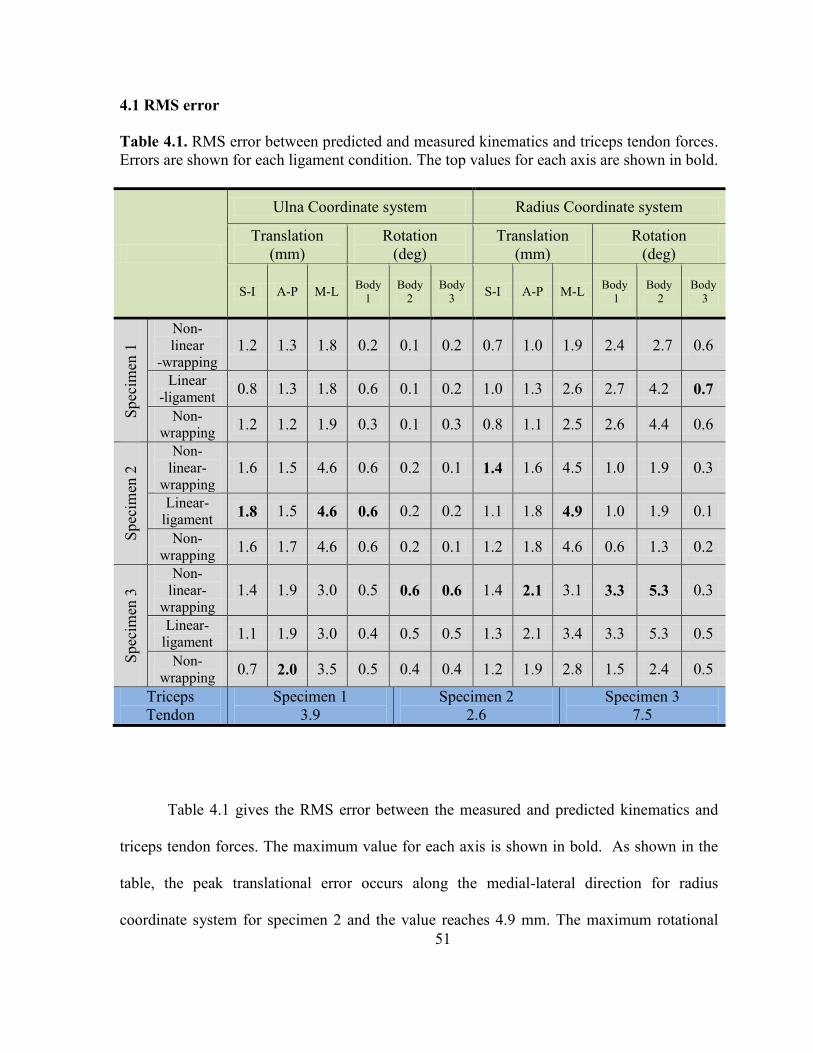
4.1 RMS error
Table 4.1. RMS error between predicted and measured kinematics and triceps tendon forces.
Errors are shown for each ligament condition. The top values for each axis are shown in bold.
Ulna Coordinate system Radius Coordinate system
Translation
(mm)
Rotation
(deg)
Translation
(mm)
Rotation
(deg)
S-I A-P M-L Body
1
Body
2
Body
3 S-I A-P M-L
Body
1
Body
2
Body
3
Spec
imen
1
Non-
linear
-wrapping 1.2 1.3 1.8 0.2 0.1 0.2 0.7 1.0 1.9 2.4 2.7 0.6
Linear
-ligament 0.8 1.3 1.8 0.6 0.1 0.2 1.0 1.3 2.6 2.7 4.2 0.7
Non-
wrapping 1.2 1.2 1.9 0.3 0.1 0.3 0.8 1.1 2.5 2.6 4.4 0.6
Spec
imen
2
Non-
linear-
wrapping 1.6 1.5 4.6 0.6 0.2 0.1 1.4 1.6 4.5 1.0 1.9 0.3
Linear-
ligament 1.8 1.5 4.6 0.6 0.2 0.2 1.1 1.8 4.9 1.0 1.9 0.1
Non-
wrapping 1.6 1.7 4.6 0.6 0.2 0.1 1.2 1.8 4.6 0.6 1.3 0.2
Spec
imen
3
Non-
linear-
wrapping 1.4 1.9 3.0 0.5 0.6 0.6 1.4 2.1 3.1 3.3 5.3 0.3
Linear-
ligament 1.1 1.9 3.0 0.4 0.5 0.5 1.3 2.1 3.4 3.3 5.3 0.5
Non-
wrapping 0.7 2.0 3.5 0.5 0.4 0.4 1.2 1.9 2.8 1.5 2.4 0.5
Triceps
Tendon
Specimen 1
3.9
Specimen 2
2.6
Specimen 3
7.5
Table 4.1 gives the RMS error between the measured and predicted kinematics and
triceps tendon forces. The maximum value for each axis is shown in bold. As shown in the
table, the peak translational error occurs along the medial-lateral direction for radius
coordinate system for specimen 2 and the value reaches 4.9 mm. The maximum rotational

52
error of 5.3° occurs for specimen 3 for body 2 rotation of the radius coordinate system. The
largest translational error for the ulna happens along the medial-lateral direction for specimen
3 and the value reach 4.6mm. The largest rotation error for the ulna occurs in the body 1
rotation of the 123 sequence (internal/external rotation) for specimen 2 (0.6°). The greatest
RMS error is 7.5N for the triceps tendon force in specimen 3.
4.2 Ulna kinematics
Figure 4.1. Superior-inferior (S-I) displacement of the ulna coordinate system relative to the
humerus coordinates for specimen 1.
53
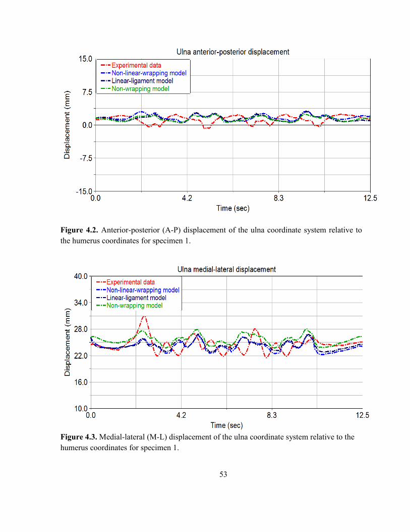
Figure 4.2. Anterior-posterior (A-P) displacement of the ulna coordinate system relative to
the humerus coordinates for specimen 1.
Figure 4.3. Medial-lateral (M-L) displacement of the ulna coordinate system relative to the
humerus coordinates for specimen 1.

54
Figures 4.1-4.3 provide the S-I, A-P, and M-L displacements of ulna coordinate
system relative to the humerus coordinate system respectively and presented in humerus
coordinate. The magnitude of S-I and A-P displacement is comparatively small and reached a
maximum range of 3mm. The value for M-L displacement is greater than S-I and M-L
displacement values and the range extend to about 8mm. The predicted results of ulna
displacements are an average agreement with the experimental values, and the maximum
RMS error (1.8 mm) occurs in M-L direction.
Figure 4.4. Ulna internal-external (I-E) rotation relative to the humerus coordinates for
specimen 1.

55
Figure 4.5. Ulna adduction-abduction (AD-AB duction) relative to the humerus coordinates
for specimen 1.
Figure 4.6. Ulna flexion-extension (F-E) relative to the humerus coordinates for specimen 1.

56
The presented figures 4.4-4.6 shown above provide the comparison between the body
1, 2, 3 orientations of ulna coordinate system relative to the humerus coordinate system about
the x, y and z-axes of humerus coordinate system respectively. The orientation magnitudes
are higher from their corresponding displacement magnitude. The body 3 orientation angle of
the ulna relative to the humerus represents the flexion-extension (F-E) of the forearm. The
value for F-E is the highest for the angles and ranged to nearly 20°. The angle values for
body 1 and 2 are smaller than body 3. The angel range was approximately 5° for body 1 and
8° for body 2. The body 1 and 2 rotations represent the internal-external (I-E) and adduction-
abduction (AD-AB duction ) of the ulna relative to humerus respectively. As illustrated in the
figures, the predicted results of ulna orientations are in a good agreement with the
experimental values throughout the period of study.
4.3 Radius kinematics
Figure 4.7. S-I displacement of the radius coordinate system relative to the humerus
coordinates for specimen 1.
57
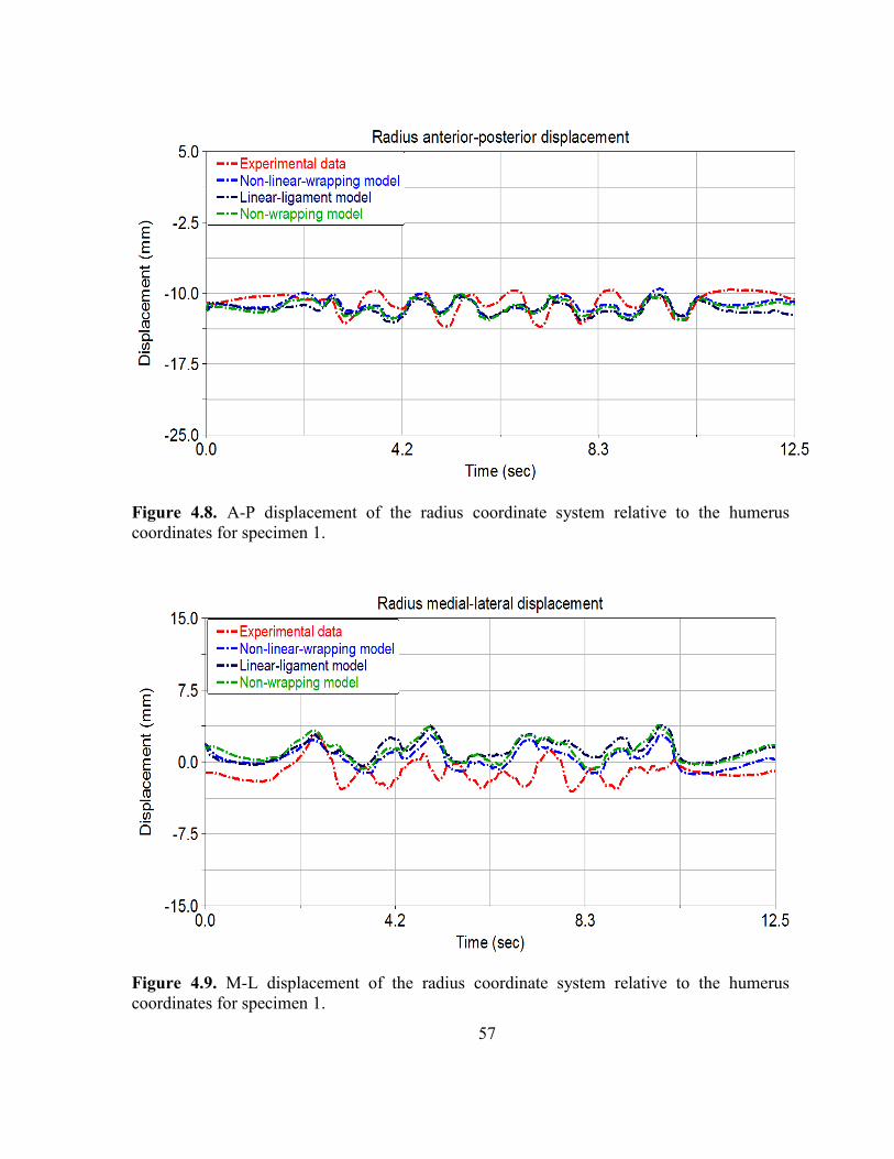
Figure 4.8. A-P displacement of the radius coordinate system relative to the humerus
coordinates for specimen 1.
Figure 4.9. M-L displacement of the radius coordinate system relative to the humerus
coordinates for specimen 1.

58
Figures 4.7-4.9 provides the S-I, A-P and M-L displacement of radius coordinate
system relative to the humerus coordinate system respectively and presented in humerus
coordinate system. The radius displacement practically shows the similar trends with the
ulnar displacement as they are connected with the interosseous membrane and annular
ligaments. However, since the radius has more laxity and less constraint than ulna, the
magnitude of radius displacement is little bigger compare to ulna. The maximum value for
M-L displacement is 7mm; and for S-I and A-P displacements are 6mm and 4mm
respectively. It is observed from the figure that the predicted radius displacements have good
proximity with the experimental values.
Figure 4.10. Radius I-E rotation relative to the humerus coordinates for specimen 1.

59
Figure 4.11. Radius I-E rotation relative to the humerus coordinates for specimen 1
Figure 4.12. Radius AD-AB duction relative to the humerus coordinates for specimen 1.
60
The body 1, 2, 3 rotations of radius coordinate system relative to the humerus
coordinate system as shown in figures 4.10-4.12 respectively represents the I-E rotation, AD-
AB duction, and F-E of radius. Although the I-E rotation and AD-AB duction are somewhat
deviated from the experimental observation, the F-E has a very good agreement with the
experiment. The difference might be explained by a defected structure of cartilages that
produced unpredicted contact surfaces and contact forces. As presented in the figures, the
range of I-E rotation, AD-AB duction, and F-E are 12°, 10° and 20° respectively.
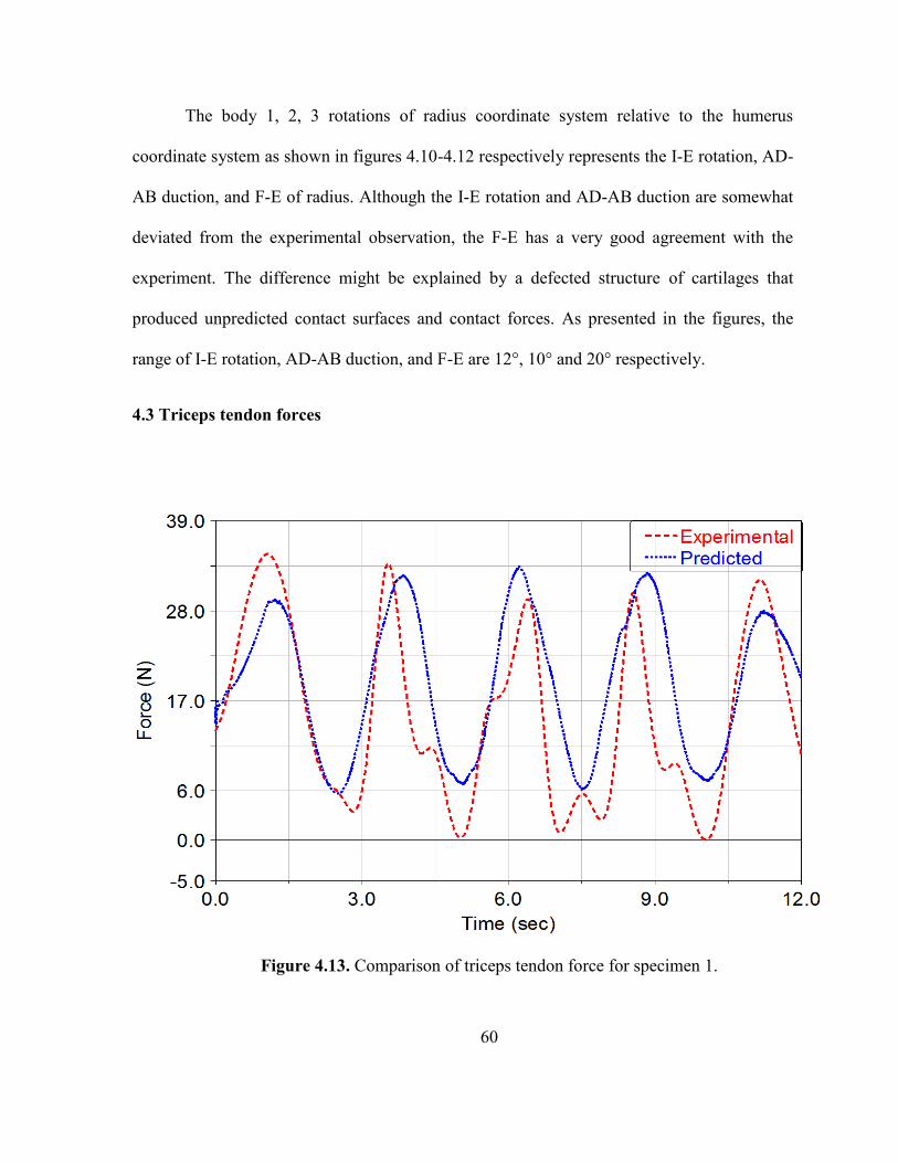
4.3 Triceps tendon forces
Figure 4.13. Comparison of triceps tendon force for specimen 1.

61
The peak triceps tendon force observed from the figure 4.13 is about 33N. As
illustrated in the figure, the triceps tendon was loaded when the elbow was flexing and
unloaded when the elbow was extending. The experimental load cell signals were smoothed
using a low-pass 2nd
order Butterworth filter with a cut-off frequency of 4Hz. The predicted
force data has nearly similar trends to the experimental measured data although some
difference was observed due to lack of accurate measurement of zero-load length and suture
stiffness parameter.
62
CHAPTER 5
DISCUSSION
The main purpose of this study was to develop and validate an anatomically correct
subject specific 3D computational multibody model of the elbow joint complex. The models
presented here were developed in the multibody framework that could be placed in neuro-
musucluloskeletal models of the upper arm. The models were validated by comparing the
predicted bone kinematics and triceps tendon force to experimentally measured data from an
identically loaded cadaver (Figs. 4.1 - 4.13). In order to quantify the model accuracy, the root
mean square errors (RMS error) between model predictions and experimental measures were
calculated. Overall, the RMS errors are small throughout the models that support a good
agreement between the models and experiments.
A small improvement in kinematics compared to experimental measurement was
observed when the lateral ulnar collateral and annular ligament were wrapped around the
bones. Some additional reductions of RMS error were also acquired when a non-linear toe
region was modeled in the ligament compared to models that had only a linear force-
displacement relationship. Although these observations were not statistically significant
(ANOVA p-value was greater than 0.05), this may suggest that ligament toe region and
ligament wrapping should be included.
Review of the literature revealed several modeling approaches for the elbow joint
(Buchanan et al., 1998; Garner & Pandy, 2001; Gonzalez et al., 1999; Gonzalez et al., 1996;
Holzbaur et al., 2005; Lemay & Crago, 1996; Raikova, 1992; Schuind et al., 1991; Triolo et

63
al., 2001). However, these models typically ignored the ligament contribution in joint
modeling. Although some studies incorporated the ligament effect in the model (Fisk &
Wayne, 2009; Spratley & Wayne, 2011), these studies ignored cartilages, ligament non-linear
property and ligament wrapping around the bone. Modeling cartilage in the joints, wrapping
the ligament around the bone, and incorporating the ligament non-linearity in the model is
the unique work presented in this study.
The modeling of annular ligament wrapping benefits simulation of the radial head
rotation. Modeling a circular path of for the annular ligament allows the radius to rotate
inside the ligament similar to its physiological motion. Furthermore, it provides the
attachment of radial collateral ligament with the annular ligament that provides the pathway
for forces to be transmitted between the lateral epicondyle and radius/lateral ulna (Fisk,
2007). Along with the ligament contributions, the contact between the articular cartilages is
essential to the elbow joint. The contact between the olecranon and olecranon fossa provides
the elbow extension limit (Morrey, 2000). In addition, contact between the coronoid process
and coronoid fossa provides significant effects on elbow flexion range of motion. Due to the
multiple contact points between the coronoid process and coronoid fossa, the computational
model here provides greater ulnohumeral contact force in elbow flexion (Fisk, 2007).
In the present study, the developed computational multibody model was able to
represent flexion-extension associated with forearm pronation-supination accurately. The
model was also able to persuasively predict joint function by providing a more detailed
description of the underlying structures. Furthermore, this model allowed prediction of
important biomechanical parameters that are difficult to measure in cadaver studies, such as
contact and ligament forces.

64
Although the results of this study are promising, differences still exist between the
model and experimental investigations. In most cases, the largest values of RMS error
occurred for the radius coordinate system relative to the humerus coordinate system. The
biggest RMS errors for translation occurred in the medial-lateral direction for the radius
relative to the humerus for specimen 2 and the value reached to 4.9 mm (Table 4.1). The
largest rotation RMS error was 5.30 adduction-abduction of the radius relative to the humerus
for specimen 3.
5.1 Study limitations
Multiple sources of modeling and experimental error exist that may have caused
differences between model prediction and experimentally measured values. Due to poor
quality of MRI, it was difficult to extract the real cartilage geometries. So, the articular
cartilage geometries were assumed to have a uniform thickness over bone surfaces. But
actual cartilage thickness is non-homogenous and varies over the bone. As a result, the
modeled contact surface will differ from the actual contact surfaces that may affect contact
magnitudes, locations and orientations, creating a source of modeling error. Furthermore,
during experiment for the large rotations of the radius, the Optotrak cameras could lose sight
of the ired markers, causing loss of kinematic data that affected the model validation.
Additionally, the model was validated only by testing the resulting joint segment motions and
triceps tendon force. Contact forces and pressures in the cadaver elbow joint were not
directly measured. In addition, the models were validated with only three specimens. A larger
sample size may help to make more generalized conclusions.

65
The inability to predict stress and strain within the tissue is a major limitation of rigid
multibody models. Predicting strain in cartilage and ligament tissues is important to
understand tissue level degeneration and disease (Bei & Fregly, 2004; Stylianou et al., 2012).
The ligament path was chosen for annular ligaments as a rigid spline that may resist the
translational movement of the radius. Including compliance contact instead of using point
curve constraint in the ligament may improve the medial-lateral translation errors of the
radius. Specimen 1 was disarticulated from the distal radioulnar joint, reducing constraints
for the radius and introducing unexpected movements. However, these limitations had been
overcome by using the steel dynamic compression plate for specimen 2 and 3. Finally, the bi-
axial mechanical tester had a limited range of motion (50mm) that producing small changes
in flexion angle during experimental testing. A larger range of motion evaluating the elbow
joint is important to understand ligament characteristics.
5.2 Future work
Various future works could be explored for this model such as; adding non-uniform
discrete cartilage, more ligament wrapping, incorporating ligament viscoelastic properties,
adding more muscle force and muscle contractile properties, and build a full musculoskeletal
model of upper extremities. Discretizing the cartilage would make it possible to predict
contact pressures in the cartilage during loading profiles. As a result, valuable insight about
the joint functions and developing better surgical technique for cartilage deficiency could be
attainable. To get a more generalized idea about model prediction and to intensify the model
validation, a larger sample size would be recommended. It is also recommended to use the
large value of flexion-extension to understand the ligament contribution in joint stability.

66
This modeling work is the first step in developing a musculoskeletal model of the
elbow joint. The developed model will then be used for subject specific full musculoskeletal
movement simulations of the upper-extremity.
5.3 Conclusion
The computational multibody model has been developed and validated by comparing
the simulated results with the experimental investigations. The models can predict some
parameters that are difficult to investigate experimentally, such as forces within ligaments
and contact forces between cartilages covered bones. While these results are promising,
further refinements of model parameters may increase its accuracy and applicability. The
models presented here were developed in the multibody framework that will be finally
incorporate into the neuro-musucluloskeletal models of the upper arm.
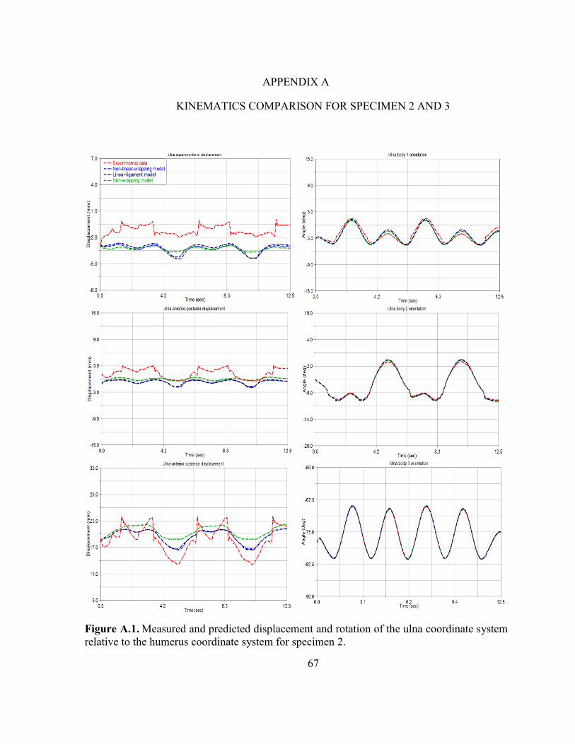
67
APPENDIX A
KINEMATICS COMPARISON FOR SPECIMEN 2 AND 3
Figure A.1. Measured and predicted displacement and rotation of the ulna coordinate system
relative to the humerus coordinate system for specimen 2.

68
Figure A.2 Measured and predicted displacement and rotation of the radius coordinate
system relative to the humerus coordinate system for specimen 2.
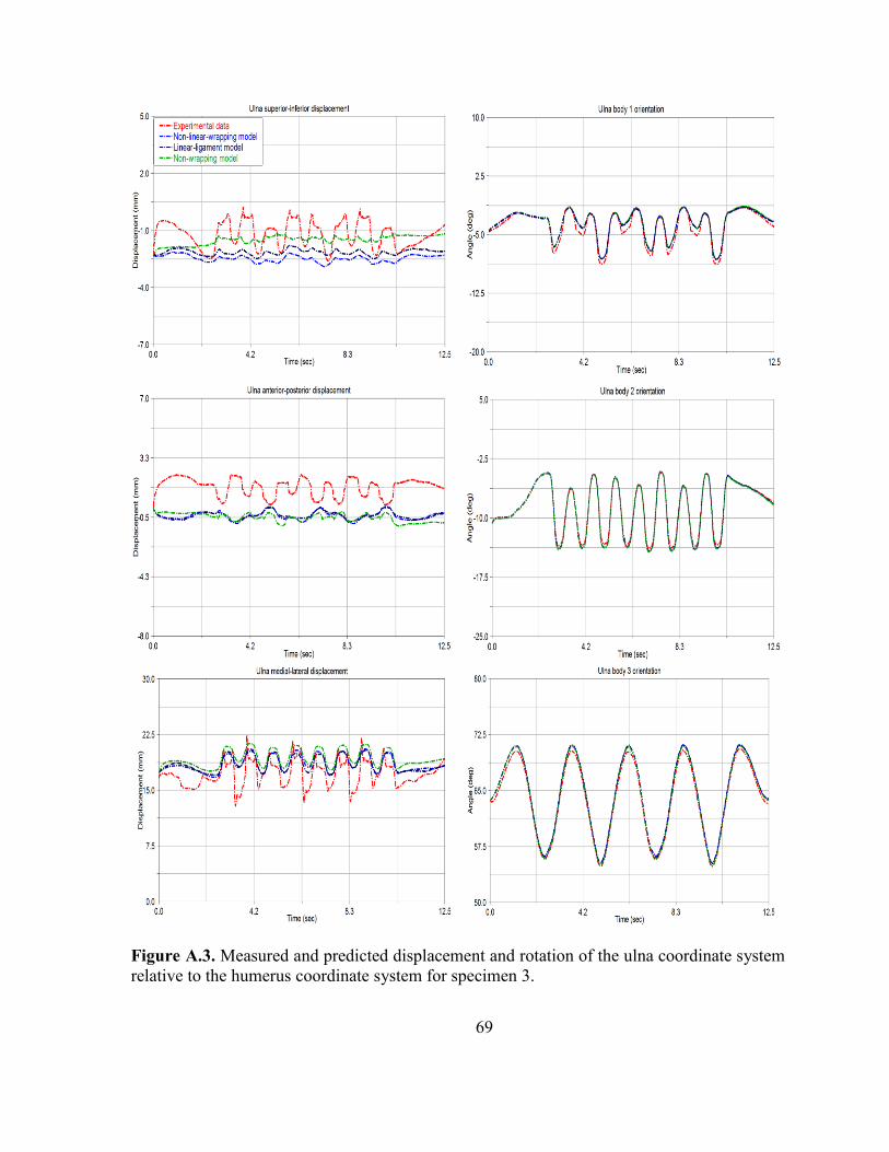
69
Figure A.3. Measured and predicted displacement and rotation of the ulna coordinate system
relative to the humerus coordinate system for specimen 3.
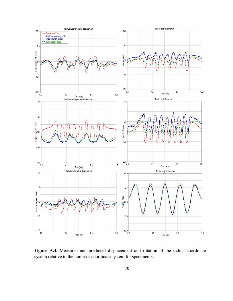
70
Figure A.4. Measured and predicted displacement and rotation of the radius coordinate
system relative to the humerus coordinate system for specimen 3.
71
REFERENCES
Alcid, J. G., Ahmad, C. S., & Lee, T. Q. (2004). Elbow anatomy and structural
biomechanics. Clin Sports Med, 23(4), 503-517, vii. doi: 10.1016/j.csm.2004.06.008
Amis, A., Dowson, D., & Wright, V. (1979). Muscle strengths and musculoskeletal geometry
of the upper limb. Engineering in Medicine, 8(1), 41-48.
An, K. N. (2005). Kinematics and constraint of total elbow arthroplasty. J Shoulder Elbow
Surg, 14(1 Suppl S), 168S-173S. doi: 10.1016/j.jse.2004.09.035
Anderson, F. C., & Pandy, M. G. (2001). Dynamic optimization of human walking. J
Biomech Eng, 123(5), 381-390.
Arnold, A. S., & Delp, S. L. (2001). Rotational moment arms of the medial hamstrings and
adductors vary with femoral geometry and limb position: implications for the
treatment of internally rotated gait. J Biomech, 34(4), 437-447. doi: 10.1016/s0021-
9290(00)00232-3
Barker, T. M., Kirtley, C., & Ratanapinunchai, J. (1997). Calculation of multi-segment rigid
body joint dynamics using MATLAB. Proc Inst Mech Eng H, 211(6), 483-487.
Bei, Y., & Fregly, B. J. (2004). Multibody dynamic simulation of knee contact mechanics.
Med Eng Phys, 26(9), 777-789. doi: 10.1016/j.medengphy.2004.07.004
Benham, M. P., Wright, D. K., & Bibb, R. (2001). Modelling soft tissue for kinematic
analysis of multi-segment human body models. Biomed Sci Instrum, 37, 111-116.
Blankevoort, L., Kuiper, J. H., Huiskes, R., & Grootenboer, H. J. (1991). Articular contact in
a three-dimensional model of the knee. J Biomech, 24(11), 1019-1031.
Bloemker, K. H., Guess, T. M., Maletsky, L., & Dodd, K. (2012). Computational knee
ligament modeling using experimentally determined zero-load lengths. Open Biomed
Eng J, 6, 33-41. doi: 10.2174/1874230001206010033
72
Buchanan, T. S., Delp, S. L., & Solbeck, J. A. (1998). Muscular resistance to varus and
valgus loads at the elbow. J Biomech Eng, 120(5), 634-639.
Chao, E. Y., Armiger, R. S., Yoshida, H., Lim, J., & Haraguchi, N. (2007). Virtual
Interactive Musculoskeletal System (VIMS) in orthopaedic research, education and
clinical patient care. J Orthop Surg Res, 2, 2. doi: 10.1186/1749-799x-2-2
Chaudhari, A. M., & Andriacchi, T. P. (2006). The mechanical consequences of dynamic
frontal plane limb alignment for non-contact ACL injury. J Biomech, 39(2), 330-338.
doi: 10.1016/j.jbiomech.2004.11.013
Chuang, L. L., Wu, C. Y., Lin, K. C., & Lur, S. Y. (2012). Quantitative mechanical
properties of the relaxed biceps and triceps brachii muscles in patients with subacute
stroke: a reliability study of the myoton-3 myometer. Stroke Res Treat, 2012, 617694.
doi: 10.1155/2012/617694
Cohen, M. S., & Bruno, R. J. (2001). The collateral ligaments of the elbow: anatomy and
clinical correlation. Clin Orthop Relat Res(383), 123-130.
Cohen, Z. A., Henry, J. H., McCarthy, D. M., Mow, V. C., & Ateshian, G. A. (2003).
Computer simulations of patellofemoral joint surgery. Patient-specific models for
tuberosity transfer. Am J Sports Med, 31(1), 87-98.
Currier, D. P. (1972). Maximal isometric tension of the elbow extensors at varied positions. I.
Assessment by cable tensiometer. Phys Ther, 52(10), 1043-1049.
de Haan, J., Schep, N. W., Eygendaal, D., Kleinrensink, G. J., Tuinebreijer, W. E., & den
Hartog, D. (2011). Stability of the elbow joint: relevant anatomy and clinical
implications of in vitro biomechanical studies. Open Orthop J, 5, 168-176. doi:
10.2174/1874325001105010168
Degreef, I., & De Smet, L. (2011). The arthroscopic ulnohumeral arthroplasty: from mini-
open to arthroscopic surgery. Minim Invasive Surg, 2011, 798084. doi:
10.1155/2011/798084
Delp, S. L., & Loan, J. P. (1995). A graphics-based software system to develop and analyze
models of musculoskeletal structures. Comput Biol Med, 25(1), 21-34.

73
Donahue, T. L., Hull, M. L., Rashid, M. M., & Jacobs, C. R. (2002). A finite element model
of the human knee joint for the study of tibio-femoral contact. J Biomech Eng,
124(3), 273-280.
Fernandez, J. W., & Pandy, M. G. (2006). Integrating modelling and experiments to assess
dynamic musculoskeletal function in humans. Exp Physiol, 91(2), 371-382. doi:
10.1113/expphysiol.2005.031047
Ferreira, L. M., (2011). Development of an Active Elbow Motion Simulator and Coordinate
Systems to Evaluate Kinematics in Multiple Positions. Paper 84.
Ferreira, L. M., King, G. J., & Johnson, J. A. (2011). Motion-derived coordinate systems
reduce inter-subject variability of elbow flexion kinematics. J Orthop Res, 29(4), 596-
601. doi: 10.1002/jor.21278
Fisk, J. P. (2007). Development and validation of a computational musculoskeletal model of
the elbow joint. Virginia Commonwealth University. Richmond, Virginia
Fisk, J. P., & Wayne, J. S. (2009). Development and validation of a computational
musculoskeletal model of the elbow and forearm. Ann Biomed Eng, 37(4), 803-812.
doi: 10.1007/s10439-009-9637-x
Freund, J., & Takala, E. P. (2001). A dynamic model of the forearm including fatigue. J
Biomech, 34(5), 597-605.
Fuss, F. K. (1991). The ulnar collateral ligament of the human elbow joint. Anatomy,
function and biomechanics. J Anat, 175, 203-212.
Garner, B. A., & Pandy, M. G. (2001). Musculoskeletal model of the upper limb based on the
visible human male dataset. Comput Methods Biomech Biomed Engin, 4(2), 93-126.
doi: 10.1080/10255840008908000
Gavronski, G., Veraksits, A., Vasar, E., & Maaroos, J. (2007). Evaluation of viscoelastic
parameters of the skeletal muscles in junior triathletes. Physiol Meas, 28(6), 625-637.
doi: 10.1088/0967-3334/28/6/002
Giddings, V. L., Beaupre, G. S., Whalen, R. T., & Carter, D. R. (2000). Calcaneal loading
during walking and running. Med Sci Sports Exerc, 32(3), 627-634.
74
Gonzalez, R. V., Abraham, L. D., Barr, R. E., & Buchanan, T. S. (1999). Muscle activity in
rapid multi-degree-of-freedom elbow movements: solutions from a musculoskeletal
model. Biol Cybern, 80(5), 357-367.
Gonzalez, R. V., Andritsos, M. J., Barr, R. E., & Abraham, L. D. (1993). Comparison of
experimental and predicted muscle activation patterns in ballistic elbow joint
movements. Biomed Sci Instrum, 29, 9-16.
Gonzalez, R. V., Hutchins, E. L., Barr, R. E., & Abraham, L. D. (1996). Development and
evaluation of a musculoskeletal model of the elbow joint complex. J Biomech Eng,
118(1), 32-40.
Guess, T. M. (2012). Forward dynamics simulation using a natural knee with menisci in the
multibody framework. Multibody System Dynamics, 28(1-2), 37-53. doi:
10.1007/s11044-011-9293-4
Guess, T. M., Liu, H., Bhashyam, S., & Thiagarajan, G. (2013). A multibody knee model
with discrete cartilage prediction of tibio-femoral contact mechanics. Comput
Methods Biomech Biomed Engin, 16(3), 256-270. doi:
10.1080/10255842.2011.617004
Guess, T. M., & Stylianou, A. (2012). Simulation of anterior cruciate ligament deficiency in
a musculoskeletal model with anatomical knees. Open Biomed Eng J, 6, 23-32. doi:
10.2174/1874230001206010023
Guess, T. M., Thiagarajan, G., Kia, M., & Mishra, M. (2010). A subject specific multibody
model of the knee with menisci. Med Eng Phys, 32(5), 505-515. doi:
10.1016/j.medengphy.2010.02.020
Hirokawa, S. (1991). Three-dimensional mathematical model analysis of the patellofemoral
joint. J Biomech, 24(8), 659-671.
Holzbaur, K. R., Murray, W. M., & Delp, S. L. (2005). A model of the upper extremity for
simulating musculoskeletal surgery and analyzing neuromuscular control. Ann
Biomed Eng, 33(6), 829-840.

75
Hotchkiss, R. N., An, K. N., Sowa, D. T., Basta, S., & Weiland, A. J. (1989). An anatomic
and mechanical study of the interosseous membrane of the forearm: pathomechanics
of proximal migration of the radius. J Hand Surg Am, 14(2 Pt 1), 256-261.
Hunt, K. H., & Crossley, F. R. E. (1975). Coefficient of Restitution Interpreted as Damping
in Vibroimpact. Journal of Applied Mechanics, 42(2), 440. doi: 10.1115/1.3423596
Hutchins, E. L., Gonzalez, R. V., & Barr, R. E. (1993). Comparison of experimental and
analytical torque-angle relationships of the human elbow joint complex. Biomed Sci
Instrum, 29, 17-24.
Identify the muscles crossing the elbow joint. (2013). Retrieved 11/5/2013, from http://www.usi.edu/science/biology/mkhopper/2401/01Ex14MuscleAnatomy/IDElbowJoint.htm
Iwasaki, N., Genda, E., Barrance, P. J., Minami, A., Kaneda, K., & Chao, E. Y. (1998).
Biomechanical analysis of limited intercarpal fusion for the treatment of Kienbock's
disease: a three-dimensional theoretical study. J Orthop Res, 16(2), 256-263. doi:
10.1002/jor.1100160213
Kwak, S. D., Blankevoort, L., & Ateshian, G. A. (2000). A Mathematical Formulation for 3D
Quasi-Static Multibody Models of Diarthrodial Joints. Comput Methods Biomech
Biomed Engin, 3(1), 41-64. doi: 10.1080/10255840008915253
Lemay, M. A., & Crago, P. E. (1996). A dynamic model for simulating movements of the
elbow, forearm, an wrist. J Biomech, 29(10), 1319-1330.
Li, G., Gil, J., Kanamori, A., & Woo, S. L. (1999). A validated three-dimensional
computational model of a human knee joint. J Biomech Eng, 121(6), 657-662.
Liacouras, P. C., & Wayne, J. S. (2007). Computational modeling to predict mechanical
function of joints: application to the lower leg with simulation of two cadaver studies.
J Biomech Eng, 129(6), 811-817. doi: 10.1115/1.2800763
Lin, H. T., Nakamura, Y., Su, F. C., Hashimoto, J., Nobuhara, K., & Chao, E. Y. (2005). Use
of virtual, interactive, musculoskeletal system (VIMS) in modeling and analysis of
shoulder throwing activity. J Biomech Eng, 127(3), 525-530.

76
McGinley, J. C., & Kozin, S. H. (2001). Interosseous membrane anatomy and functional
mechanics. Clin Orthop Relat Res(383), 108-122.
Morey-Klapsing, G., Arampatzis, A., & Bruggemann, G. P. (2005). Joint stabilising response
to lateral and medial tilts. Clin Biomech (Bristol, Avon), 20(5), 517-525. doi:
10.1016/j.clinbiomech.2005.01.008
Morrey, B. F. (2000). The elbow and its disorders. N.B. Saunders. Independent square west.
Philadelphia, PA.
Morrey, B. F., & An, K. N. (1985). Functional anatomy of the ligaments of the elbow. Clin
Orthop Relat Res(201), 84-90.
Morrey, B. F., & Chao, E. Y. (1976). Passive motion of the elbow joint. J Bone Joint Surg
Am, 58(4), 501-508.
Murray, W. M., Delp, S. L., & Buchanan, T. S. (1995). Variation of muscle moment arms
with elbow and forearm position. J Biomech, 28(5), 513-525.
Nagano, A., Komura, T., Yoshioka, S., & Fukashiro, S. (2005). Contribution of non-extensor
muscles of the leg to maximal-effort countermovement jumping. Biomed Eng Online,
4, 52. doi: 10.1186/1475-925x-4-52
Netter, F. H., & Hansen, J. T. (2003). Atlas of human anatomy (3rd ed.). Teterboro, N.J.:
Icon Learning Systems.
Peck, C. C., Langenbach, G. E., & Hannam, A. G. (2000). Dynamic simulation of muscle
and articular properties during human wide jaw opening. Arch Oral Biol, 45(11), 963-
982.
Piazza, S. J., & Delp, S. L. (2001). Three-dimensional dynamic simulation of total knee
replacement motion during a step-up task. J Biomech Eng, 123(6), 599-606.
Pigeon, P., Yahia, L., & Feldman, A. G. (1996). Moment arms and lengths of human upper
limb muscles as functions of joint angles. J Biomech, 29(10), 1365-1370.

77
Raikova, R. (1992). A general approach for modelling and mathematical investigation of the
human upper limb. J Biomech, 25(8), 857-867.
Raikova, R. (1996). A model of the flexion-extension motion in the elbow joint some
problems concerning muscle forces modelling and computation. J Biomech, 29(6),
763-772.
Regan, W. D., Korinek, S. L., Morrey, B. F., & An, K. N. (1991). Biomechanical study of
ligaments around the elbow joint. Clin Orthop Relat Res(271), 170-179.
Ring, D., & Jupiter, J. B. (2000). Reconstruction of posttraumatic elbow instability. Clin
Orthop Relat Res(370), 44-56.
Schuind, F., An, K. N., Berglund, L., Rey, R., Cooney, W. P., 3rd, Linscheid, R. L., & Chao,
E. Y. (1991). The distal radioulnar ligaments: a biomechanical study. J Hand Surg
Am, 16(6), 1106-1114.
Shelburne, K. B., Pandy, M. G., Anderson, F. C., & Torry, M. R. (2004). Pattern of anterior
cruciate ligament force in normal walking. J Biomech, 37(6), 797-805. doi:
10.1016/j.jbiomech.2003.10.010
Shiba, R., Sorbie, C., Siu, D. W., Bryant, J. T., Cooke, T. D., & Wevers, H. W. (1988).
Geometry of the humeroulnar joint. J Orthop Res, 6(6), 897-906. doi:
10.1002/jor.1100060614
Skahen, J. R., 3rd, Palmer, A. K., Werner, F. W., & Fortino, M. D. (1997). The interosseous
membrane of the forearm: anatomy and function. J Hand Surg Am, 22(6), 981-985.
doi: 10.1016/s0363-5023(97)80036-6
Spratley, E. M., & Wayne, J. S. (2011). Computational model of the human elbow and
forearm: application to complex varus instability. Ann Biomed Eng, 39(3), 1084-
1091. doi: 10.1007/s10439-010-0224-y
Stylianou, A. P., Guess, T. M., & Cook, J. L. (2012). Development and validation of a multi-
body model of the canine stifle joint. Comput Methods Biomech Biomed Engin. doi:
10.1080/10255842.2012.684243

78
Tate, P. (2012). Seeley's Principles of anatomy & physiology (2. ed.). New York, NY: McGraw-Hill.
Triolo, R. J., Werner, K. N., & Kirsch, R. F. (2001). Modeling the postural disturbances
caused by upper extremity movements. IEEE Trans Neural Syst Rehabil Eng, 9(2),
137-144. doi: 10.1109/7333.928573
van der Helm, F. C. (1994a). Analysis of the kinematic and dynamic behavior of the shoulder
mechanism. J Biomech, 27(5), 527-550.
van der Helm, F. C. (1994b). A finite element musculoskeletal model of the shoulder
mechanism. J Biomech, 27(5), 551-569.
Wiesel, S. W., & Delahay, J. N. (2010). Essentials of Orthopedic Surgery: Springer.
Wismans, J., Veldpaus, F., Janssen, J., Huson, A., & Struben, P. (1980). A three-dimensional
mathematical model of the knee-joint. J Biomech, 13(8), 677-685.
Woo, S. L., Debski, R. E., Wong, E. K., Yagi, M., & Tarinelli, D. (1999). Use of robotic
technology for diathrodial joint research. J Sci Med Sport, 2(4), 283-297.
Wu, J. Z., Dong, R. G., Smutz, W. P., & Schopper, A. W. (2003). Modeling of time-
dependent force response of fingertip to dynamic loading. J Biomech, 36(3), 383-392.
Zielinska, B., & Donahue, T. L. (2006). 3D finite element model of meniscectomy: changes
in joint contact behavior. J Biomech Eng, 128(1), 115-123.

79
VITA
Md Munsur Rahman was born March 1, 1985 in Joypurhat, Bangladesh. He attended
Kalai M.U. High school, a local public school and finished his tenth grade in 2001. The same
year, he enrolled at the Kalai Degree College and graduated with “outstanding honors” in
2003. The following year, he entered in the Bangladesh University of Engineering and
Technology (BUET) and began studying mechanical engineering. In the fall of 2008, he
graduated with a Bachelor of Science degree in Mechanical Engineering.
After finishing the graduation, he started working with a famous refrigeration and air
condition manufacturing company in Bangladesh. There, he had a chance to work closely
with the manufacturing process and obtained a firsthand experience on industrial
environment. After getting admission in University of Missouri-Kansas City in spring 2012
semester, he moved to the United States and started pursuing his M.S in Mechanical
Engineering, with an emphasis in Biomechanics.
In January 2012, Munsur joined the Musculoskeletal Biomechanics Research
Laboratory as a graduate research assistant and spent two full years working in the
biomechanical lab under the direction of Dr. Trent Guess. Throughout his academic years, he
gained considerable experience at developing a multi-body modeling of human elbow joints.
Upon completion of his degree requirements for a Master of Science degree in Mechanical
Engineering, Munsur plans to use his education to follow a career in biomechanics.