Development and Testing of a Wind Simulator at an Operating Wind Farm

R. J. Conzemius1, H. Lu2, L. Chamorro2, Y.-T. Wu2, and F. Porte-Agel2,3

1. Introduction The minimization of wind turbine wake impacts is one of the primary considerations in wind

farm design. Yet, due to the turbulent nature of wakes, they are often rather difficult to model,

and the problem becomes particularly challenging when large arrays are planned, due to the

potential for multiple interactions among wakes. The cumulative effects of upstream turbines

can have a substantial impact on both wind farm output as well as site suitability.

Numerous models exist for characterizing wind turbine wakes (Barthalmie et al. 2006). Due

to the great computational expense of explicitly simulating turbine wakes, these models employ

great simplifications in order to make it possible to optimize the layout of large wind turbine

arrays by calculating cumulative wake effects for a myriad of different possible configurations.

Bartholmie et al. (2003, 2006) have tested these models at offshore wind farms, but validation at

various onshore wind farms is rather limited.

In more recent years, computational fluid dynamics (CFD) has become more widely accepted

as a tool for estimating wind turbine multiple wake impacts at large wind farms. This larger

acceptance has come about largely due to the continuing rapid increase in computer power and

storage capacity. However, CFD has not been extensively evaluated within large wind farm

arrays. In particular, the parameterizations used in CFD to calculate the impacts of turbulence on

the mean flow have not been thoroughly tested for atmospheric applications, and the depth of

many CFD domains has been chosen only with the height of the rotor in mind, as opposed to

considering the entire depth over which turbulent flows occur in the atmosphere. In particular,

the relevance of large, organized turbulent structures in the atmospheric boundary layer and their

role in wake meandering and recovery has not been studied. The vertical transport of momentum

and heat accomplished by these large-scale turbulent eddies in the boundary layer is not well

represented by turbulence models.

In the present study, we use large eddy simulation (LES) methodology to resolve these larger

turbulent structures so that their impacts on the mean flow in addition to the development and

dissipation of wind turbine wakes can be explicitly calculated. To focus the LES evaluation

specifically on atmospheric turbulence and its effects on turbine wakes and to avoid the

1 WindLogics, Inc. Grand Rapids, Minnesota, USA 2 Saint Anthony Falls Laboratory, University of Minnesota, Minneapolis, Minnesota, USA 3 Ecole Polytechnique Federale de Lausanne, Switzerland

Corresponding author e-mail address: bobc@windlogics.com

complicating effects of topography, we have chosen for our study a wind farm located in

relatively simple terrain. The wind farm provided supervisory control and data acquisition

(SCADA) data on a turbine-by-turbine level every 10 minutes. Additionally, we placed two

sodar instruments in the farm with the intent of measuring both the free-stream (unwaked) air

flow and the turbine wakes.

By taking measurements of turbine wakes, we also seek to further test the application of LES

methodology to simulate multiple wind turbine wakes. The code to be used for these exercises

(Porté-Agel et al. 2000, Porté-Agel 2004, Stoll and Porté-Agel 2006, Wan et al. 2007, Stoll and

Porté-Agel 2008) has already been tested extensively and compared to both wind tunnel results

and atmospheric observations. These wind tunnel tests have more recently included model wind

turbines and their wakes. However, the spectrum of turbulence in the tunnel is limited by the

width and depth of the wind tunnel, and we would like to further validate the code for

commercial scale wind turbines operating under the full spectrum of atmospheric turbulence. In

particular, the counter-rotational effect of rotor torque has been found to be significant in the

wind tunnel measurements and in LES runs that have included blade torque in the turbine

parameterization. It remains to be seen whether these effects are present and measureable in

operating wind farms. Thus, one goal of the present study is to provide further tests of the LES

methodology applied to operating wind farms and to evaluate the skill of simulations to

reproduce the velocity profile in wind turbine wakes and to discover whether wake

characteristics measured in the wind tunnel differ greatly from those experiencing the full scale

of atmospheric turbulence.

2. Experimental setup

a. Wind Farm Location The wind farm location chosen for our simulations is located in Mower County, Minnesota and

is operated by NextEra Energy Resources, Inc. The farm contains 43 Siemens SWT2.3-93

turbines (see Fig. 1), each with a peak capacity of 2.3 MW, and has been operating since late

2007. In the summer and fall of 2009, we collected SCADA data from the farm. The SCADA

data provide 10-minute averages of ambient atmospheric temperature and wind speed at the

nacelle, power output, blade pitch angle, and rotor RPM. In general, the wind farm layout was

designed to minimize wake impacts for the two prevailing wind directions at the site, which are

from the northwest and from the south. For this reason, we focused our analysis on the

southwestern portion of the farm, where one wind turbine row is oriented more north to south

than the others and is therefore more likely to experience turbine wake effects. Due to the fact

that measurement equipment could only be placed on turbine access roads within the farm, this

southwestern segment was an ideal monitoring location because the row curves at a nearly 90-

degree angle, making it possible to measure waked and unwaked wind profiles within this row

simultaneously.

Fig. 1. Layout of the wind farm and placement of the sodars in the southwest segment.

b. Sodar Data We placed two SecondWind Triton sodars within this wind turbine segment (see Fig. 1) in order

to measure the unwaked and waked wind speed profiles. The first was placed midway between

Turbines 39 (T39) and 40 (T40) with the intention of measuring the background atmospheric

wind profile during periods when the wind is coming from the south, which is one of two

prevailing wind directions for the site. The second sodar was placed between T41 and T42, but

as close to T42 as possible, in order to measure downstream wake impacts from T41.

The sodars measure the vertical wind profile using three beams, each 10 degrees off the vertical,

and separated horizontally by 120 degrees. The half power beam width is approximately 11

degrees. The Tritons are typically deployed so that one of the three beams points directly south.

Pulses from each of these three beams are sent out at approximately 10 second intervals, and the

return signals are averaged over a 10-minute period to calculate the vertical wind profile. The

profile includes all three components of velocity at heights of 40, 50, 60, 80, 100, 120, 140, 160,

180, and 200 meters above ground level (AGL). Additionally, an estimate of turbulence

intensity at each of these levels is included. A barometer is also contained within the unit as well

as a thermometer at the 2-meter level on the outside edge of the dish so that air density can be

calculated for each 10-minute observation. The sodars were deployed on July 31, 2009 and

remained operating in the wind farm until December 14, 2009.

c. Data analysis technique In the wind tunnel (Chamorro and Porte-Agel 2009), the turbulent and time-averaged

components of velocity were measured using a fast-response hot wire probe that could be moved

to any position relative to the wind turbine location, and the air flow and vertical temperature

gradient within the tunnel could be precisely controlled. The measurements provided vertical

cross-sections and profiles of mean wind and turbulence properties for neutral atmospheric

conditions. In the wind farm, such control over the wind and temperature and measurement

locations is not possible, so it is necessary to use a compositing technique to construct the wake

vertical profiles and cross sections from all measurements available throughout the course of the

field measurement campaign. It is possible to categorize the measurements in terms of

Richardson number, nocturnal versus convective boundary layer conditions, or more simply in

terms of the atmospheric temperature gradient. However, due to sampling size limitations, it was

not possible to restrict the measurements to a precise set of conditions as was done in the wind

tunnel. Therefore, some variation in conditions (for example, a composite formed using

measurements with a similar vertical temperature gradient may have had different temperatures

and different wind speeds) within any of the constructed composites was an undesired yet

necessary result.

We used a cylindrical coordinate system for our analyses, with range (meters), azimuth

(degrees), and height (meters above ground level) as the three coordinates and the zero azimuth

pointed in the direction of the upwind turbine, which, in our presented analyses, is Turbine 41

(WT41—hereafter we shall denote wind turbines by the letters ‗WT‘ followed by the turbine

number). For the SCADA data, whose variables are all measured at 80 meters AGL, the

analyses are presented as functions of azimuth only. Analyses based on sodar data are presented

as a function of both azimuth and height above ground level.

In order to classify the data according to atmospheric stability, we calculated the vertical

temperature gradient by taking the difference between the average of the nacelle ambient

temperature measurements (from all 43 turbines) and the average of the two sodar temperatures

and dividing by the 78 meter difference in height between those two levels. The vertical

temperature gradient affects wake recovery by impacting the amount of background atmospheric

turbulence, whose role is to remove velocity gradients in the flow. As the vertical temperature

gradient increases, the atmospheric conditions become less supportive of turbulence, and wakes

persist farther downstream. The largest vertical temperature gradients are found at night, when

temperature often increases with height, turbulence is generally suppressed, and the wakes are

most easily measured. In an unstable profile, when the temperature gradient is less than -10 deg

C/km, buoyancy production of turbulence occurs, and large turbulent structures cause wake

meandering and rapid dissipation of wakes. The vertical temperature gradient values in Table 1

were used as limits of our stability categories.

Table 1. Temperature Gradient Ranges Used for Stability Classification

Stability Class Temperature Gradient (K/km)

A,B <-1.7

C -1.7<x<-1.5

D -1.5<X<-0.55

E -0.55<X<1.5

F 1.5<X<100

In order to focus on occurrences of more meaningful wake impacts, we eliminated any time

periods when either the upstream or waked turbine was offline or when the wind speed was too

light for both turbines to be producing at least 150 kW power. Likewise, if the wind speed was

large enough for either turbine to reach the maximum power of 2300 kW (meaning that one or

both turbines might be operating on the upper, flat part of the power curve), we eliminated that

time period from the analysis. Imposing this upper limit on wind speed also simplified the

turbine parameterization in LES by allowing a fixed blade pitch angle near zero because the

blade pitch does not increase from zero until the turbine is operating at peak capacity. We

thereby eliminated measurements if the blade pitch angle became greater than zero degrees, and

because this happens only at or near the top of the power curve, we used blade pitch angle as a

proxy for maximum power.

The yaw angle of the ―downstream‖ turbine was used as the wind direction for all measurements,

and the compass direction terminology was used. Under such terminology, angles increase in the

clockwise direction and decrease in the counterclockwise.

Prior to performing the calculations, we corrected the yaw angles from the SCADA data. The

correction procedure was needed in order to remove yaw angle offsets that developed in the

archiving system as a result of turbine downtime (for fault conditions, maintenance, or other

reasons). When turbines are subsequently brought back online, the yaw angle is erroneously

recorded as unchanged from its previous uptime value, even when the actual yaw angle has

changed. These errors appear to be a result of archival software design.

In order to construct vertically consistent sodar cross-sections and vertical profiles, we limited

our analysis to times when the entire vertical profile was available. This occurred only 19% of

the time, but the length of the data collection period allowed a sufficient number of

measurements to be collected to form a composite cross section.

d. Large eddy simulation methodology

i. Description of the code

The LES approach explicitly solves the scales of motion larger than the grid resolution (on the

order of 10 m), while the effect of the sub-grid scales (ranging from the grid scale to the

Kolmogorov scale, on the order of 1 mm in the atmospheric boundary layer) need to be

parameterized. Two types of sub-grid models are adopted in the current work: (i) subgrid-scale

models to parameterize the effects of the unresolved turbulent eddy motions, and (ii) wind-

turbine models to parameterize the turbine-induced lift and drag forces.

Large eddy simulations are performed using recently developed scale-dependent Lagrangian

dynamic approach, which is able to account, without tuning, for the effects of local shear and

flow anisotropy on the distribution of the SGS model coefficients (Porté-Agel et al. 2000, Porté-

Agel 2004, Stoll and Porté-Agel 2006, Wan et al. 2007, Stoll and Porté-Agel 2008). The model

overcomes the limitations of traditional models in the near-wall region and delivers improved

predictions of energy spectra, mean velocity profiles as well as other characteristics at different

heights from the ground.

Wind turbine loads are calculated using the actuator disk model (ADM) and the actuator line

model (ALM). The ADM distributes the force loading on the rotor disk; and the ALM distributes

the forces on lines that follow the blade positions and thus it has the strength to capture important

characteristics of the wind turbine wake such as tip vortices and coherent periodic structures in

helical wakes (Sørensen and Shen 2002).

ii. Wind Tunnel Tests of the Code

The wind tunnel measurements of wind turbine wakes are further described in Chamorro and

Porte-Agel (2009). Prior to the application of LES to the wind farm, the LES code was tested in

a wind tunnel environment. A model wind turbine array was constructed at the wind tunnel at

the Saint Anthony Falls Laboratory (SAFL) at the University of Minnesota. The array consisted

of model wind turbines at approximately 1/800 scale mounted on the floor of the tunnel. The tip

speed ratio (λ=4) was adjusted to match that of field-scale turbines (usually between 3.5 and 6).

The tunnel is a closed loop circuit with a plan length of 37.5 m and a main test section 16 m

long, 1.7 m wide, and 1.7 m in depth. The temperature of the lower surface can be precisely

controlled using a series of aluminum strips placed within the floor of the wind tunnel. The

precise control is achieved by pumping a temperature-regulated fluid through the strips. In

addition, the air temperature can be controlled using a heat exchanger mounted in the wind

tunnel expansion after the fan. The regulated temperatures of the air and the test section floor

determine the type of boundary layer that will affect the turbine array. A picture of a model wind

turbine array in the wind tunnel is shown in Fig. 2.

The turbulence is measured by a fast-response 3-wire anemometry. The sensor (a combination of

an x-type hot-wire and a single cold-wire) was used to obtain high resolution and simultaneous

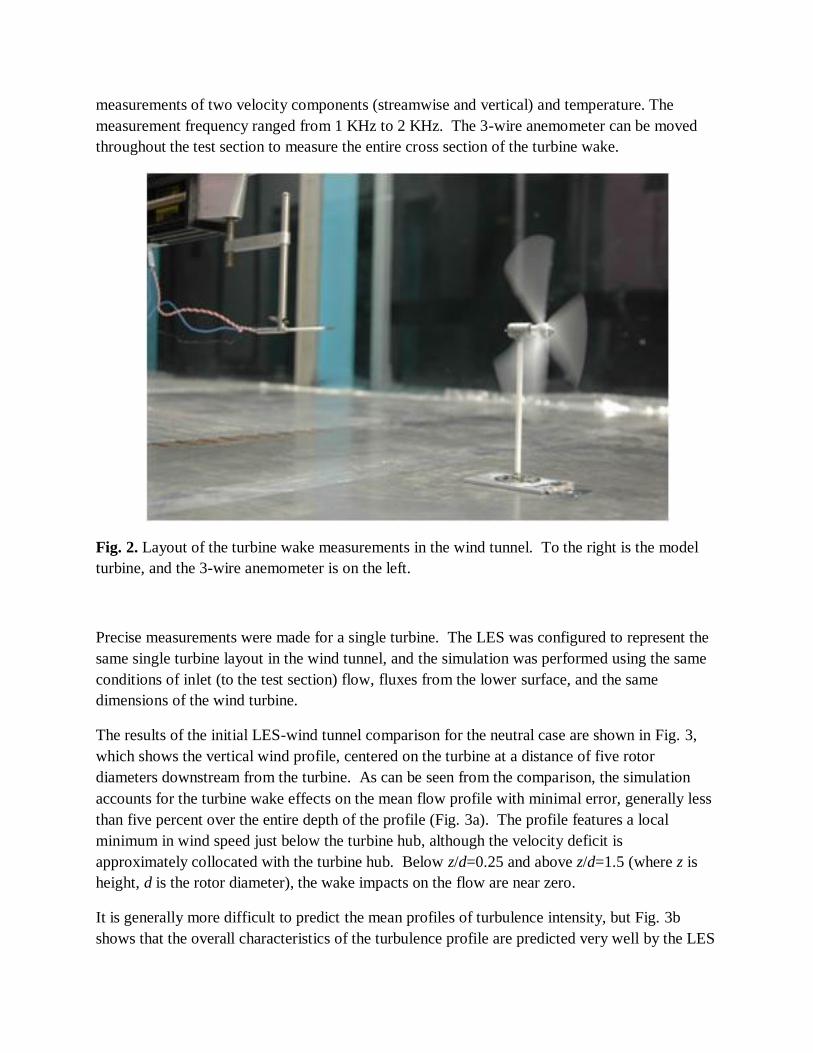
measurements of two velocity components (streamwise and vertical) and temperature. The

measurement frequency ranged from 1 KHz to 2 KHz. The 3-wire anemometer can be moved

throughout the test section to measure the entire cross section of the turbine wake.

Fig. 2. Layout of the turbine wake measurements in the wind tunnel. To the right is the model

turbine, and the 3-wire anemometer is on the left.

Precise measurements were made for a single turbine. The LES was configured to represent the

same single turbine layout in the wind tunnel, and the simulation was performed using the same

conditions of inlet (to the test section) flow, fluxes from the lower surface, and the same

dimensions of the wind turbine.

The results of the initial LES-wind tunnel comparison for the neutral case are shown in Fig. 3,

which shows the vertical wind profile, centered on the turbine at a distance of five rotor

diameters downstream from the turbine. As can be seen from the comparison, the simulation

accounts for the turbine wake effects on the mean flow profile with minimal error, generally less

than five percent over the entire depth of the profile (Fig. 3a). The profile features a local

minimum in wind speed just below the turbine hub, although the velocity deficit is

approximately collocated with the turbine hub. Below z/d=0.25 and above z/d=1.5 (where z is

height, d is the rotor diameter), the wake impacts on the flow are near zero.

It is generally more difficult to predict the mean profiles of turbulence intensity, but Fig. 3b

shows that the overall characteristics of the turbulence profile are predicted very well by the LES

code. Compared to the inflow profile (upstream from the turbine), the turbulence intensity

increases the most near the top of the rotor, where the wind shear experiences a local (in height)

maximum. The wake tip vortices may be most pronounced at this level. A very small decrease

in turbulence intensity occurs near the bottom of the blade-swept depth, likely because of the

decrease in vertical shear there, causing a decrease in mechanical turbulence production.

Fig. 3. 3-wire anemometry measurements of the center of the turbine wake at a downwind

distance of five rotor diameters: (a) mean vertical wind profile; and (b) profile of the standard

deviation of the x-component of velocity (u) scaled by hub height mean flow (uhub).

e. Measurements Used for LES Initialization in Operating Wind Farm

We selected a temporally contiguous set of measurements when WT41 and WT42 were

operating and when Triton169 was, during at least some portion of the selected time interval,

measuring a wake. Unlike the compositing procedure described above, it was not necessary to

restrict the analyses to time intervals when sodars were providing a full or nearly full vertical

profile of measurements, but it was necessary to have measurements up to at least 140 m AGL in

order for the entire wake profile to be measured. Within the selected time period (November 22,

2009), variations of wind speed and direction and temperature occurred, making it possible to

sample different locations in the cross section of the wake. The LES was initialized using the

unwaked profiles measured by Triton172, supplemented with gridded analysis data from the

Rapid Update Cycle (RUC) model at heights above the maximum measurement in the sodar

vertical profile. The temperature was constructed using the 2-meter sodar temperature (average

between the two sodars), the average of the 43 SCADA measurements of temperature taken at

the 80-meter level, and temperature from the RUC levels above 200 m AGL. Linear

interpolation was used between these levels to bring the measurements to the grid vertical levels.

Wind speed horizontal components were interpolated linearly between the lowest sodar level (40

m AGL) and all subsequent levels above that. RUC horizontal wind component data were used

at levels above the sodar measurements. In the lowest 40 meters, the wind was assumed to have

a logarithmic vertical profile with a friction velocity of 0.63 m/s and a surface roughness of 0.3

m.

In order to provide the turbulent component of LES inlet conditions that are representative of

the atmospheric conditions at the time, an LES pre-run was conducted without wind turbines, the

results were saved, and the pre-run data were used as the inlet (south boundary) condition for the

run with the wind turbines. The lateral (east-west) boundary conditions were chosen as periodic,

and the outlet condition (on the north side) was a Neumann zero gradient condition.

3. Results

a. SCADA Analysis Wind turbine wakes are not necessarily seen in the data during individual instances of waking.

Rather, the SCADA data reveal wakes when viewed in a composite manner with all available

observations taken during the course of the field measurement campaign. We show the data by

calculating the ratios of wind speed and power from the SCADA data from WT42 and WT41 in

order to indicate the velocity deficit. Although a large amount of scatter is obvious in the plots

(Fig. 4), if the data points are binned in five-degree increments (red lines), the wakes are more

clearly seen in the data When WT42 is waked, the ratio of the WT42 to WT41 wind speeds

drops below unity. When WT41 is waked and WT42 is unwaked, the ratio becomes larger than

one. It is possible to see the evidence of waking from various pairs of turbines in the row.

However, only neighboring turbines appear to have an impact on each other in these plots. Due

to the roughly cubic nature of the relationship between wind speed and power over the range of

wind speeds considered, plots of power ratio as a function of wind direction (Fig. 4b) show

larger peaks and valleys and also more scatter in the ratio, but overall, the power data confirm

the relationships among turbines shown by the wind speed data.

Atmospheric stability plays a large role in the scatter of the data points due to its impact on

background atmospheric turbulence (Fig. 5). When the background atmospheric temperature

profile is unstable (Fig. 5a), there is considerably larger scatter in the power ratio, making it

difficult to detect the wake impacts, even when the data are binned. The results are strongly

indicative of the role of atmospheric turbulence in bringing about the breakup of turbine wakes

during unstable conditions, when the production of atmospheric turbulence due to buoyancy

effects is rather pronounced. On the opposite end of the stability scale (Fig. 5b), wake impacts

are more pronounced, relative to the background scatter, when the atmospheric temperature

profile is very stable and background atmospheric turbulence is either suppressed or its length

scales reduced. In either case, the impact on turbine wakes is much less, and they persist farther

downstream.

Fig. 4. Ratio of WT42 to WT41 SCADA variables: (a) wind speed, and (b) active power. The

red lines denote averages of observations in 5-degree bins.

Fig. 5. Ratio of WT42:WT41 power as a function of atmospheric stability (see Table 1): (a) class

A/B, and (b) class F. The red lines denote averages of observations in 5-degree bins.

b. Sodar Data Sodar composite cross-sections can reveal the effects of multiple atmospheric processes on the

turbine wakes. One question about the wake measurements is whether or not rotational effects

-100 0 100Angle (degrees)

0

1

2

3

4

5R

atio

42

:41

win

d s

pee

d

W

T4

3 w

akin

g W

T4

2

W

T4

1 w

akin

g W

T4

2

WT

40

wa

kin

g W

T4

1

W

T4

2 w

akin

g W

T4

1(a)

-100 0 100Angle (degrees)

0

1

2

3

4

5

Ratio 4

2:4

1 p

ow

er

W

T4

3 w

akin

g W

T4

2

W

T41

wa

kin

g W

T4

2

WT40 waking WT41

WT42wakingWT41

(b)

-100 0 100Angle (degrees)

0

1

2

3

4

5

Ratio 4

2:4

1 p

ow

er

(a)

-100 0 100Angle (degrees)

0

1

2

3

4

5

Ratio 4

2:4

1 p

ow

er

(b)

exist in the wake, and if so, whether they can be detected by sodar. The cross sections of vertical

velocity (Fig. 6) suggest that the sodars have measured rotation of the turbine wake during the

experiment. Positive vertical velocity is preferentially located to the left of the wake centerline,

and negative vertical velocity is oriented more to the right, with the zero isotach slanting

downward from left to right across the wake. Although this configuration may not be purely

rotational (in particular, positive vertical velocity tends to be found at low levels under the entire

wake), the sign of rotation matches that which would be expected for the blade rotation of the

SWT2.3-93 turbines.

An additional aspect of the wake is that it appears sheared and rather oval-shaped, with the long

axis of the oval oriented from the upper left to lower right. This effect is due to the wind shear

that is most often present during nocturnal or stable conditions, when the wakes are most

pronounced. During such conditions, the wind vectors point more to the left at very low altitudes

and more to the right above (when seen in the framework moving with the flow), due to the

balance of vertical turbulent momentum exchange (otherwise known as Reynolds stresses) and

the Coriolis and pressure gradient forces. This sort of a vertical profile is consistent with the

Ekman profile: if the horizontal component of the velocity vectors were plotted on a Cartesian

axis, a spiral shape would result.

Perhaps the most noticeable characteristic of the wake is the offset of minimum velocity deficits

to the left of the so-called centerline at Y/Rd=0. We hypothesize that the positive vertical

velocity may advect smaller wind speeds from lower altitudes. Alternatively, the effects of wind

shear may simply move the deficit, which can generally be expected to occur just above the hub

height, to the left. Note that the reference wind speed is taken from the 80 meter level.

The wake recovery as a function of distance can be estimated using all of the available data from

the two operating sodars in the farm. Figure 7 shows the wind speed ratios of the sodars as a

function of wind direction. In this case, zero degrees is oriented to the north. This plot, which

we refer to as a ―sodar rose‖, reveals distinct wakes whose impacts can be roughly quantified by

taking the minimum of velocity ratio along a 30-degree arc centered on the azimuth pointing to

the turbine causing the wake. Although there are more turbines in the row than are indicated in

the sodar rose, not all of them have a discrete wake impact. In those cases, the turbine may be

too far away for the sodar to consistently measure its wake, or the wake may be too close to the

wake of another turbine to be measured as a distinct wake. For example, WT39 appears to have

no impact on Triton169 because the sodar wind speed ratio is almost exactly unity in the

direction from Triton169 to WT39.

(a)

(b)

Fig. 6. Cross sections of waked:unwaked wind speed ratio (shading) and vertical velocity (black

lines—dashed lines are negative, contour interval of 0.05 m/s) for the following pairs of turbines:

(a) WT42 (waked) and WT41 (unwaked), and (b) WT40 (waked) and WT39 (unwaked). The

rotor diameter of each turbine responsible for a velocity deficit is shown with a solid gray line.

Taking into account all the wake information from the sodar rose, as well as the distances

between the sodars and the respective turbines, one can estimate the wake as a function of

distance (Fig. 8). In general, the curve that can be inferred is that of a negative exponential

function that asymptotically approaches unity.

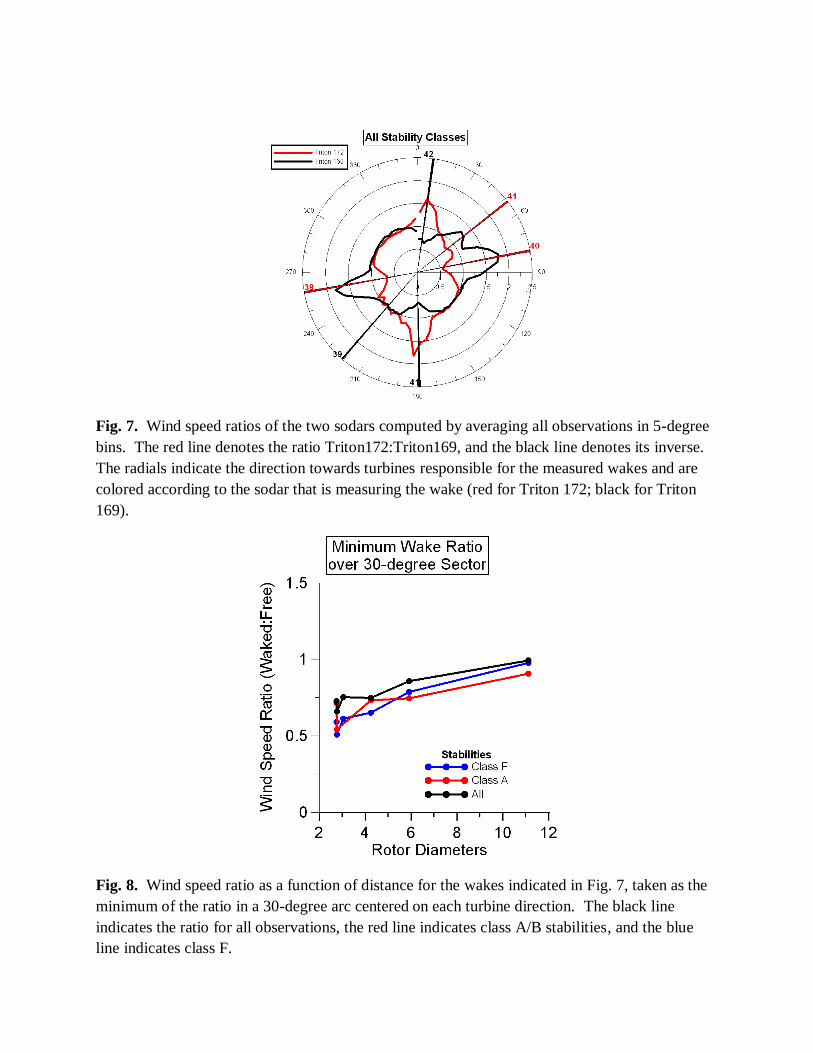
Fig. 7. Wind speed ratios of the two sodars computed by averaging all observations in 5-degree

bins. The red line denotes the ratio Triton172:Triton169, and the black line denotes its inverse.

The radials indicate the direction towards turbines responsible for the measured wakes and are

colored according to the sodar that is measuring the wake (red for Triton 172; black for Triton

169).

Fig. 8. Wind speed ratio as a function of distance for the wakes indicated in Fig. 7, taken as the

minimum of the ratio in a 30-degree arc centered on each turbine direction. The black line

indicates the ratio for all observations, the red line indicates class A/B stabilities, and the blue

line indicates class F.

We made an attempt to categorize the wake recovery according to atmospheric stability, but the

results do not have the expected stratification. One would expect a slower wake recovery with

stronger stability, but either the atmospheric stability is not having such an effect on the wakes,

or the field experiment collected an insufficient number of samples to clearly see the

relationships that exist between atmospheric stability and turbine wake recovery. We believe the

latter of these two possibilities to be true. In either case, approximately 80 percent wake

recovery has occurred by 12 rotor diameters downstream, with speed ratios there increasing to

0.9 from a minimum of 0.5 at a distance of 3 rotor diameters downstream.

c. Cumulative Wake Impacts Finally, we examine the cumulative wake impacts of multiple turbines in a row. We oriented the

SCADA analyses for WT33 through WT38 so that the zero azimuth was pointed at WT32. As is

demonstrated in the analysis (Fig. 9), the accumulation of wakes causes the velocity deficit to

grow in width and depth proceeding down the row of turbines. We averaged the wind power

ratio (WTXX:WT32) over a 30-degree width centered on zero degrees for each of these turbines,

and the results are presented in Fig. 10. We have also separated the results into the various

atmospheric stability categories. In general, the wake accumulation is more severe for more

stable conditions, which favor the persistence of wakes. In unstable conditions, greater

atmospheric turbulence favors the rapid breakup of wakes. Nevertheless, significant wake

accumulation occurs in all of the stability categories.

a. Large Eddy Simulation Case Study We chose November 22, 2009 at 2200 to 2300 UTC as a case study because of near neutral

atmospheric stability, the atmospheric conditions were favorable for good sodar echoes, and the

wind direction was from the south, which brought the wake from WT41 over Triton169. The

LES setup procedure was as described in the previous section. The simulation was set up as a

neutral ABL case with a surface roughness of z0=0.3 m, a friction velocity of u*=0.63 m/s,

domain dimensions of Lx=2100 m (including buffer zone), Ly=1350 m, and Lz=300 m at a

resolution of Nx=360, Ny=288, and Nz=64. These dimensions produce grid cells that are

approximately 5 meters on a side, allowing for approximately 20 grid points over the diameter of

the wind turbine rotor.

A snapshot of LES output on the X-Y plane at approximately 80 meters above the surface (Fig.

11) shows the turbulent nature of the flow for this case. The turbine wakes are visible, but the

velocity deficits within them are not a lot larger than the velocity fluctuations due to the

background atmospheric turbulence. The largest wind speeds are found on the inlet (left) side

upstream from the turbines, and the smallest wind speeds are found in the wake of WT42, where

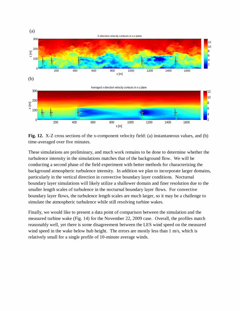
the combined wakes of WT41 and WT42 are present. An X-Z cross section taken along the

plane intersecting both WT41 and WT42 (Fig. 12a) shows a significant amount of velocity

fluctuation in the vertical direction as well. When time-averaging is applied to the flow (Fig.

12b), the wakes stand out more clearly.

Fig. 9. Ratio of the power output of the selected turbine to the power output of WT32 during all

occurrences of F class stability: (a) WT33, (b) WT34, (c) WT35, (d) WT36, (e) WT37, and (f)

WT38. The red lines denote the average of data points in five-degree bins.

-80 -40 0 40 80Angle (degrees)

0

1

2

3

4

5P

ow

er

Ra

tio

(a) WT33

-80 -40 0 40 80Angle (degrees)

0

1

2

3

4

5

Pow

er

Ra

tio

(b) WT34

-80 -40 0 40 80Angle (degrees)

0

1

2

3

4

5

Pow

er

Ra

tio

(c) WT35

-80 -40 0 40 80Angle (degrees)

0

1

2

3

4

5

Pow

er

Ra

tio

(d) WT36

-80 -40 0 40 80Angle (degrees)

0

1

2

3

4

5

Pow

er

Ra

tio

(e) WT37

-80 -40 0 40 80Angle (degrees)

0

1

2

3

4

5

Pow

er

Ra

tio

(f) WT38

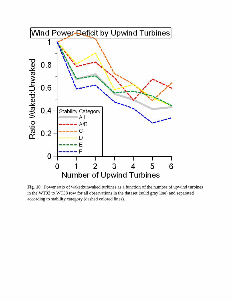
Fig. 10. Power ratio of waked:unwaked turbines as a function of the number of upwind turbines

in the WT32 to WT38 row for all observations in the dataset (solid gray line) and separated

according to stability category (dashed colored lines).

Fig. 11. X-Y cross section of the x-component of velocity for the LES of the November 22,

2009 case.

An idealized neutral simulation was also conducted with Lx=2400m (including buffer zone),

Ly=1200m, and Lz=300m at a resolution of Nx=128, Ny=128, and Nz=32 (each rotor plane

covers 10 grid points). The incoming flow was treated as neutrally stratified with z0=0.2m and

u*=0.65m/s. The time-averaged data on the X-Z plane intersecting WT41 and WT42 (Fig. 13)

show some interesting characteristics of the wakes. Fig. 13a shows the rotational component of

the flow in the turbine wakes to be on the order of 0.5 m/s. As in the case study, the largest

velocity deficit (Fig. 13b) is found downstream from WT42, where the wakes from WT41 and

WT42 combine. X-Z turbulence intensity cross sections from this simulation through the axis of

WT39 (Fig. 13c) confirm that the largest turbulence intensity in the wake is in the upper portion

where wind shear is the largest (see Fig. 13b). With combined wakes (Fig. 13d), the turbulence

intensity was larger in this simulation where wakes combined, creating larger shear at the top of

the combined wake than at the top of the single wake.

x [m]

y [m

]X-direction velocity contours in x-y plane

200 400 600 800 1000 1200 1400 1600

200

400

600

800

1000

1200

0

2

4

6

8

10

(a)

(b)

Fig. 12. X-Z cross sections of the x-component velocity field: (a) instantaneous values, and (b)

time-averaged over five minutes.

These simulations are preliminary, and much work remains to be done to determine whether the

turbulence intensity in the simulations matches that of the background flow. We will be

conducting a second phase of the field experiment with better methods for characterizing the

background atmospheric turbulence intensity. In addition we plan to incorporate larger domains,

particularly in the vertical direction in convective boundary layer conditions. Nocturnal

boundary layer simulations will likely utilize a shallower domain and finer resolution due to the

smaller length scales of turbulence in the nocturnal boundary layer flows. For convective

boundary layer flows, the turbulence length scales are much larger, so it may be a challenge to

simulate the atmospheric turbulence while still resolving turbine wakes.

Finally, we would like to present a data point of comparison between the simulation and the

measured turbine wake (Fig. 14) for the November 22, 2009 case. Overall, the profiles match

reasonably well, yet there is some disagreement between the LES wind speed on the measured

wind speed in the wake below hub height. The errors are mostly less than 1 m/s, which is

relatively small for a single profile of 10-minute average winds.

x [m]

z [m

]

X-direction velocity contours in x-z plane

200 400 600 800 1000 1200 1400 16000

100

200

300

2

4

6

8

10

12

x [m]

z [m

]

Averaged x-direction velocity contours in x-z plane

200 400 600 800 1000 1200 1400 16000

100

200

300

2

4

6

8

10

12

x [m]

z [m

]

<u'u'>1/2

contours in x-z plane

200 400 600 800 1000 1200 1400 16000

100

200

300

0.5

1

1.5

2

2.5

(a)

(b)

(c)

(d)

Fig. 13. Time-averaged (over one hour) contours along the indicated planes: (a) x-component

velocity u on the x-z plane through the axis of the 3rd

turbine; (b) y-component velocity v on the

x-z plane through the axis of the 3rd

turbine; (c) turbulence intensity (u)2 on the x-z plane

through the axis of the 1st turbine; and (d) turbulence intensity (u)

2 on the x-z plane through the

axis of the 3rd

turbine.

x

z

200 400 600 800 1000 1200 1400 1600 18000

100

200

300

-0.5

0

0.5

x

z

200 400 600 800 1000 1200 1400 1600 18000

100

200

300

4

6

8

10

12

x

z

200 400 600 800 1000 1200 1400 1600 18000

100

200

300

0.5

1

1.5

x

z

200 400 600 800 1000 1200 1400 1600 18000

100

200

300

0.5

1

1.5

50

100

150

200

4 5 6 7 8 9 10 11 12

Sodar 172 from field

Sodar 169 from field

Log-law fit (u*=0.63,z0=0.3)

Sodar 172 from LES

Sodar 169 from LES

U [m/s]

z [m

]

Fig. 14. Vertical wind speed profile comparison for the November 22, 2009 case. The unwaked

profile measured by sodar is indicated by the solid black squares, the LES counterpart is

indicated by the solid black line, and the logarithmic fit to the sodar data is shown with a thin,

dashed line. The sodar-measured waked profile is indicated with empty squares, and the LES

waked profile is the dot-dashed line.

4. Summary and Future Work The SCADA data show that wakes can be measured on land when the data are composited.

However, atmospheric turbulence plays a major role in determining how persistent and

detectable those wakes are. In unstable conditions, which are supportive of buoyancy-produced

turbulence, a deep convective boundary layer forms with large, organized structures on the order

of 1 km in size. This turbulence causes meandering and rapid destruction of wind turbine wakes.

In these conditions, the composited SCADA data show only a relatively subtle wake signature.

In stable conditions, turbulence is of a smaller length scale and relatively suppressed. Turbine

wakes in those conditions are much more persistent and are well-vidualized in the SCADA data.

Cross sections prepared from composite SODAR data, show the effects of multiple atmospheric

processes on the wakes. Some wake rotation is evident and matches the rotation that would be

expected from the rotation of the turbine blades. The oval shape of the wake reflects wind shear

that occurs during stable atmospheric conditions. Additionally, the greatest velocity deficit is

shifted up and to the left when viewed from a perspective looking upstream at the turbine

generating the wake. This displacement could be due either to the shear or to the upward

advection of slower velocity by the upward component of the turbine rotation. SODAR data also

have been used to demonstrate the recovery of wakes and show that by about 12 rotor diameters

downstream, at least 80 percent recovery has occurred.

The effect of accumulated wakes has been measured by SCADA data from a turbine row within

the farm. The accumulation of velocity deficit in the combined wakes is most significant during

the most stable atmospheric conditions. The wake accumulation is manifested in both the width

and the minimum of the velocity deficit within the wake.

LES of specific and idealized cases to date shows that the turbulent structure of the background

atmospheric flow tends to obscure the wakes. Time-averaging of this turbulent flow is necessary

to more clearly reveal the turbine wakes, which disperse relatively quickly in the turbulent flows

that have been simulated to date. The simulated wake profile from the November 22, 2009 case

shows a relatively close match with sodar data in the upper half of the profile, but the simulated

profile is slower than the measured profile in the lower portion of the wake.

A lot of simulation work remains to be done. In particular, a pre-simulation without wind

turbines is always needed to provide inflow conditions to the simulation with wind turbines. The

pre-simulation needs to be carefully checked to ensure that the time-averaged wind profiles

match the measured incoming flow, the turbulence is fully developed, and its statistics (intensity,

etc.) match the turbulence in the incoming flow. Only after these careful checks have been made

can the simulated wakes be meaningfully compared with the sodar-measured wakes. SCADA

and sodar measurements have provided strong evidence that the background atmospheric

turbulence plays a critical role in the downstream evolution of wind turbine wakes, and it is

critically important to get the atmospheric turbulence characteristics correct in order to perform

useful simulations of wind turbine wakes. Additionally, multiple simulations, encompassing a

variety of atmospheric conditions, need to be performed before the results can be interpreted in a

more general sense.

Acknowledgements This research was supported by the National Science Foundation (grant ATM-0854766), NASA (grant

NNG06GE256), customers of Xcel Energy through a grant (RD3-42) from the Renewable Development

Fund, and the University of Minnesota Institute for Renewable Energy and the Environment. Computing

resources were provided by the Minnesota Supercomputing Institute. The sodars were provided by

SecondWind, Inc., and Barr Engineering Company assisted with their deployment.

References

R. J. Barthelmie, L. Folkerts, F. T. Ormel, P. Sanderhoff, P. J. Eecen, O. Stobbe, and N. M.

Nielsen. Offshore wind turbine wakes measured by sodar. J. Atmos. and Oceanic Technol.,

20, 466-477, 2003.

R. J. Barthelmie, L. Folkerts, G. C. Larsen, K. Rados, S. C. Pryor, S. T. Frandsen, B. Lange, and

G. Schepers. Comparison of wake model simulations with offshore wind turbine wake

profiles measured by sodar. J. Atmos. and Oceanic Technol., 23:888-901, 2006.

L. P. Chamorro and F. Porte-Agel, F. A wind tunnel investigation of turbine wakes: boundary

layer turbulence effects. Boundary Layer Meteorol., 132:129-149, 2009.

F. Porte-Agel, C. Meneveau, and M. B. Parlange. A scale-dependent dynamics model for large-

eddy simulation: an application to the atmospheric boundary layer. J. Fluid. Mech., 415:261-

284, 2000.

F. Porté -Agel. A scale-dependent dynamic model for scalar transport in large-eddy simulations

of the atmospheric boundary layer. Boundary Layer Meteorol., 112:81–105, 2004.

R. Stoll and F. Porté-Agel. Effect of roughness on surface boundary conditions for large-eddy

simulation. Boundary Layer Meteorol., 118:169–187, 2006.

R. Stoll and F. Porté-Agel. Large-eddy simulation of the stable atmospheric boundary layer using

dynamic models with different averaging schemes, Boundary-Layer Meteorol., 126:1-28,

2008

F. Wan, F. Porté-Agel, and R. Stoll. Evaluation of dynamic subgrid-scale models in large-eddy

simulations of neutral turbulent flow over a two-dimensional sinusoidal hill. Atmos. Env.,

doi: 10.1016/j.atmosenv.2006.11.054, 1–10, 2007.

J. N. Sørensen and W. Z. Shen. Numerical modeling of wind turbine wakes. J. Fluids Eng.,

124:393–399, 2002.