University of South CarolinaScholar Commons

Theses and Dissertations

1-1-2013

Development and Figures of Merit ofMicroextraction and Ultra-Performance LiquidChromatography for Forensic Characterization ofDye Profiles on Trace Acrylic, Nylon, Polyester, andCotton Textile FibersScott James HoyUniversity of South Carolina

Follow this and additional works at: https://scholarcommons.sc.edu/etd

Part of the Chemistry Commons

This Open Access Dissertation is brought to you by Scholar Commons. It has been accepted for inclusion in Theses and Dissertations by an authorizedadministrator of Scholar Commons. For more information, please contact dillarda@mailbox.sc.edu.

Recommended CitationHoy, S. J.(2013). Development and Figures of Merit of Microextraction and Ultra-Performance Liquid Chromatography for ForensicCharacterization of Dye Profiles on Trace Acrylic, Nylon, Polyester, and Cotton Textile Fibers. (Doctoral dissertation). Retrieved fromhttps://scholarcommons.sc.edu/etd/2391

Development and Figures of Merit of Microextraction and Ultra-Performance Liquid

Chromatography for Forensic Characterization of Dye Profiles on Trace Acrylic, Nylon,

Polyester, and Cotton Textile Fibers

By

Scott J. Hoy

Bachelor of Science

Georgia Institute of Technology, 2005

Submitted in Partial Fulfillment of the Requirements

For the Degree of Doctor of Philosophy in

Chemistry and Biochemistry

College of Arts and Sciences

University of South Carolina

2013

Accepted by:

Stephen L. Morgan, Major Professor

Scott R. Goode, Committee Member

Michael L. Myrick, Committee Member

James M. Chapman, Committee Member

Lacy Ford, Vice Provost and Dean of Graduate Studies

ii

© Copyright by Scott James Hoy, 2013

All Rights Reserved.

iii

DEDICATION

This work is dedicated to my family for their unwavering love and support.

iv

ABSTRACT

Methodology for the microextraction of basic dyes on acrylic, acid dyes on nylon,

disperse dyes on polyester, and reactive dyes, direct dyes, and indigo on cotton textile

fibers is reported. Although these processes are destructive to the fiber evidence, the

ability to analyze dye extracts from sub-millimeter fiber lengths of single fibers, coupled

with detection limits in the hundred picogram range by ultra-performance liquid

chromatography (UPLC) with both diode array detection (DAD) and tandem mass

spectrometry (MS-MS) makes routine forensic characterization feasible.

Microextraction, followed by UPLC, can often distinguish similar fibers containing

different, but similar, dyes with the combination of retention time matching, UV/visible

spectral comparison, and structural analysis by mass spectrometry. This work focuses on

determining the optimum extraction conditions for each dye class and developing

chromatographic methods with suitable resolution and sensitivity for trace analysis.

Analysis of fibers as small as 1 mm in length is the target sample size to minimize

destruction of fiber evidence. Analytical figures of merit and validation statistics,

including extraction reproducibility, linearity, limits of detection and quantitation, and

UPLC precision, are reported.

The analysis of cotton fibers is challenging because they can be dyed with three

different classes of dye, each requiring a different method for extraction and analysis.

Reactive dyes present a unique challenge because they are chemically bound to the

cellulose structure of the fiber. Release of these dyes from cotton requires breaking of the

covalent bond using hot sodium hydroxide. The resulting hydrolysis reactions can also

cleave amide bonds and possibly other chemical bonds in the dye molecule. The various

v

structural changes that can take place leads, in many cases, to production of multiple

reaction products from a single dye. We demonstrate successful extraction of reactive

dyes from single 1 mm cotton fibers with detection limits as low as 3.3 pg. Systematic

experiments at varying reaction conditions, with product analysis by mass spectrometry,

were also performed to characterize the degradation of reactive dyes under hydrolysis,

and to facilitate interpretation of reactive dye extractions.

The concept of the sensitivity ratio as an analytical performance characteristic was

introduced by John Mandel of the National Bureau of Standards in 1954, but has been not

been widely applied in analytical chemistry. The basis for Mandel sensitivity is reviewed

here, along with examples of its use. Because the sensitivity ratio is independent of the

scale in which measurements are expressed, it is a useful tool for comparisons of

variability between different analytical methods.

vi

TABLE OF CONTENTS

Dedication ......................................................................................................................... iii

Abstract ............................................................................................................................. iv

List of Tables .................................................................................................................... vii

List of Figures ..................................................................................................................viii

Chapter One: Trace Chemical Analysis of Dyes Extracted from

Forensic Evidence Fibers: A Review ......................................................................1

Chapter Two: Comprehensive Screening of Acid, Basic, And

Disperse Dyes Extracted from Millimeter-Length Trace Evidence

Fibers by Ultra-Performance Liquid Chromatography:

Methodology and Figures of Merit ....................................................................... 20

Chapter Three: Extraction of Direct and Indigo Dyes from

Trace Cotton Fibers for Forensic Characterization by

Ultra-Performance Liquid Chromatography ......................................................... 65

Chapter Four: Extraction and Characterization of Reactive

Dyes and Their Hydrolysis Products from Trace Cotton Fibers

by Ultra-Performance Liquid Chromatography .................................................... 96

Chapter Five: Mandel Sensitivity Applied to Analytical Method

Performance Comparisons and Limits of Detection ............................................128

Works Cited .....................................................................................................................144

vii

LIST OF TABLES

Table 1.1 Limits of detection for food dyes determined by

HPLC-DAD and UPLC-DAD .............................................................................. 19

Table 2.1 List of textile dyes, molecular structures, and

UV/visible absorbance spectra .............................................................................. 36

Table 2.2 Mobile phase gradient profiles ......................................................................... 38

Table 2.3 MS-MS transitions and voltage settings ........................................................... 39

Table 2.4 Summary of the calibration and LOD results ................................................... 40

Table 2.5 Summary of the calibration and LOQ results ................................................... 40

Table 3.1 Structures and spectra of the direct dyes and indigo ........................................ 79

Table 3.2 Solvent compositions for each design point for the

extraction optimization for direct-dyed cotton fibers ........................................... 80

Table 3.3 Mobile phase conditions for the analysis of direct dyes by UPLC ................... 81

Table 3.4 Mobile phase conditions for the analysis of indigo by UPLC .......................... 82

Table 3.5 Peak retention time and area reproducibility for 1 cm fibers

dyed with Direct Blue 80 ...................................................................................... 83

Table 3.6 Limits of detection and quantitation of the direct and indigo dyes .................. 84

Table 3.7 Peak areas for four 5 mm fiber extracts for Direct Blue 71 .............................. 85

Table 4.1 Structures and absorbance spectra for the reactive dyes ..................................108

Table 4.2 Mobile phase conditions for the analysis of reactive dyes by UPLC ..............109

Table 4.3 Limits of detection and quantitation of the reactive dyes ................................110

viii

LIST OF FIGURES

Figure 2.1 Fiber guillotine for cutting fibers down to 5 mm in length ............................. 41

Figure 2.2 Separation of acid, basic, and disperse dyes at 1 ppm concentration .............. 42

Figure 2.3 UPLC-DAD chromatograms for Acid Blue 281 extracted

from a 0.5 mm fiber (top), 1 mm fiber (middle), and 5 mm fiber (bottom) ......... 43

Figure 2.4 UPLC-DAD chromatograms for Acid Red 337 extracted

from a 0.5 mm fiber (top), 1 mm fiber (middle), and 5 mm fiber (bottom) ......... 44

Figure 2.5 UPLC-DAD chromatograms for Acid Yellow 49 extracted

from a 1 mm fiber (top) and a 5 mm fiber (bottom) ............................................. 45

Figure 2.6 UPLC-DAD chromatograms for Basic Red 46 extracted

from a 0.5 mm fiber (top), 1 mm fiber (middle), and 5 mm fiber (bottom) ......... 46

Figure 2.7 UPLC-DAD chromatograms for Basic Violet 16 extracted

from a 0.5 mm fiber (top), 1 mm fiber (middle), and 5 mm fiber (bottom) ......... 47

Figure 2.8 UPLC-DAD chromatograms for Basic Yellow 28 extracted

from a 0.5 mm fiber (top), 1 mm fiber (middle), and 5 mm fiber (bottom) ......... 48

Figure 2.9 UPLC-DAD chromatograms for Disperse Violet 77 extracted

from a 0.5 mm fiber (top), 1 mm fiber (middle), and 5 mm fiber (bottom) ......... 49

Figure 2.10 UPLC-DAD chromatograms for Disperse Yellow 114 extracted

from a 0.5 mm fiber (top), 1 mm fiber (middle), and 5 mm fiber (bottom) ......... 50

Figure 2.11 UPLC-DAD chromatograms for Disperse Blue 60 extracted

from a 0.5 mm fiber (top), 1 mm fiber (middle), and 5 mm fiber (bottom) ......... 51

Figure 2.12 High concentration UPLC-DAD calibration plot for Acid Blue 281 ............ 52

Figure 2.13 Low concentration UPLC-DAD calibration plot for Acid Blue 281 ............ 52

Figure 2.14 UPLC-MS-MS Calibration plot for Acid Blue 281 ...................................... 53

ix

Figure 2.15 High concentration UPLC-DAD calibration plot for Acid Red 337 ............. 53

Figure 2.16 Low concentration UPLC-DAD calibration plot for Acid Red 337.............. 54

Figure 2.17 UPLC-MS-MS Calibration plot for Acid Red 337 ....................................... 54

Figure 2.18 High concentration UPLC-DAD calibration plot for Acid Yellow 49.......... 55

Figure 2.19 Low concentration UPLC-DAD calibration plot for Acid Yellow 49 .......... 55

Figure 2.20 UPLC-MS-MS Calibration plot for Acid Yellow 49 .................................... 56

Figure 2.21 High concentration UPLC-DAD calibration plot for Basic Red 46 .............. 56

Figure 2.22 Low concentration UPLC-DAD calibration plot for Basic Red 46 .............. 57

Figure 2.23 UPLC-MS-MS Calibration plot for Basic Red 46 ........................................ 57

Figure 2.24 High concentration UPLC-DAD calibration plot for Basic Violet 16 .......... 58

Figure 2.25 Low concentration UPLC-DAD calibration plot for Basic Violet 16 ........... 58

Figure 2.26 UPLC-MS-MS calibration plot for Basic Violet 16 ...................................... 59

Figure 2.27 High concentration UPLC-DAD calibration plot for Basic Yellow 28 ........ 59

Figure 2.28 Low concentration UPLC-DAD calibration plot for Basic Yellow 28 ......... 60

Figure 2.29 UPLC-MS-MS Calibration plot for Basic Yellow 28 ................................... 60

Figure 2.30 High concentration UPLC-DAD calibration plot for Disperse Blue 60........ 61

Figure 2.31 UPLC-MS-MS Calibration plot for Disperse Blue 60 .................................. 61

Figure 2.32 High concentration UPLC-DAD calibration plot for Disperse Violet 77 ..... 62

Figure 2.33 Low concentration UPLC-DAD calibration plot for Disperse Violet 77 ...... 62

Figure 2.34 UPLC-MS-MS Calibration plot for Disperse Violet 77 ................................ 63

Figure 2.35 High concentration UPLC-DAD calibration plot for

Disperse Yellow 114 ............................................................................................. 63

Figure 2.36 Low concentration UPLC-DAD calibration plot for

Disperse Yellow 114 ............................................................................................. 64

x

Figure 2.37 UPLC-MS-MS calibration plot for Disperse Yellow 114 ............................. 64

Figure 3.1 Reduction of indigo to its water-soluble leuco form ....................................... 86

Figure 3.2 Perspective view (left) and contour plot (right) of fitted absorbance

response surface for direct dye extraction as a function of solvent conditions.

Design points from Table 3.2 are indicated by solid dots.

A, Water; B, Pyridine; C, Acetone ....................................................................... 87

Figure 3.3 Optical microscope image (magnification12.5) of cotton fibers

dyed with Direct Orange 39 .................................................................................. 88

Figure 3.4 Fitted linear absorbance response surface for Indigo extraction

as a function of solvent conditions Design points follow those from

Table 4.2 and are indicated by solid dots.

A, DMSO; B, Chloroform; C, Pyridine ................................................................ 89

Figure 3.5 Chromatogram showing the separation of all three direct dyes.

Some dyes have multiple components. Peak 1 is Direct Blue 80,

peak 2 is Direct Blue 71, and peak 3 is Direct Orange 39 .................................... 90

Figure 3.6 Multiple direct dye component in the chromatographic region

of 1 to 2.5 min from Figure 3.5. Peak 1 is Direct Blue 80, peak 2 is

Direct Blue 71, peak 3 is Direct Orange 39, and peaks labeled ―D‖

are miscellaneous dye stuff ................................................................................... 91

Figure 3.7 UPLC-DAD chromatogram of Indigo ............................................................. 92

Figure 3.8 Calibration relationship for Direct Blue 80 ..................................................... 93

Figure 3.9 Chromatogram of 1 mm Direct Blue 71 dye peak from 1.6-2.0 min .............. 94

Figure 3.10 Chromatogram of the extraction of Indigo from a 1 mm cotton fiber........... 95

Figure 4.1 Worldwide consumption of cotton dyes .........................................................111

Figure 4.2 Mechanism for the dyeing of cellulose by Reactive Orange 72 .....................112

Figure 4.3 Mechanism showing the extraction of Reactive Orange 72

from cellulose, and further dye hydrolysis due to excess NaOH .........................113

Figure 4.4 Chromatogram showing the separation of all three reactive

dyes. Some dyes have multiple components. Peak 1 is Reactive

Blue 220, peak 2 is Reactive Orange 72, and peak 3 is Reactive

Yellow 160 ...........................................................................................................114

xi

Figure 4.5 Multiple reactive dye components in the chromatographic

region of 0.8 to 2.6 min from Figure 4. Peaks labeled with a 1 are

Reactive Blue 220, peaks labeled with a 2 are Reactive Orange 72,

and peaks labeled with a 3 are Reactive Yellow 160 ...........................................115

Figure 4.6 (Left) UPLC chromatograms for Reactive Orange 72

standard and (right) extracted (standard treated with NaOH and heat) ...............116

Figure 4.7 Areas of both peaks observed after treatment of Reactive

Orange 72 with varying amounts of NaOH. 100% represents

9.375e-7 moles of NaOH to 1 ng of dye 117 .......................................................117

Figure 4.8 Total ion chromatogram of Reactive Yellow 160 standard

and isolated molecular ions of four dye derivatives ............................................118

Figure 4.9 Total ion chromatogram of the Reactive Yellow 160 standard,

isolated molecular ions of the potential dye derivatives, and their

corresponding UV/visible absorbance spectra .....................................................119

Figure 4.10 TIC of Reactive Yellow 160 after being treated with NaOH

and heat (100°C). Two products were visible by HPLC-MS ..............................120

Figure 4.11 TIC of Reactive Orange 72 showing the only visible

chromatographic peak and its mass spectra .........................................................121

Figure 4.12 Extracted ion chromatograms for m/z 572, 474, 492,

and 417 from the analysis of Reactive Orange 72. Individual

chromatographic peaks for each mass suggest multiple

compounds present in the standard ......................................................................122

Figure 4.13 TIC and mass spectra of Reactive Orange 72 after treatment

with NaOH and heat (100°C) ...............................................................................123

Figure 4.14 Calibration model for Reactive Blue 220 .....................................................124

Figure 4.15 Calibration Model for Reactive Orange 72 ..................................................125

Figure 4.16 Calibration Model for Reactive Yellow 160 ................................................126

Figure 4.17 UPLC-DAD chromatograms of extracted Reactive

Yellow 160 from a 10 mm fiber (top), a 5 mm fiber (middle) and

a 1 mm fiber (bottom) ..........................................................................................127

Figure 5.1 Calibration relationship for two different measurement processes ................141

xii

Figure 5.2 Calibration relationship for two different measurement

processes with noise; standard deviation for upper (blue) calibration is

5 counts, and the standard deviation for the lower (red)

calibration is 2 counts ..........................................................................................141

Figure 5.3 Calibration relationship for the first method with plus

and minus one standard deviation window about the response

of 25 peak counts for 25 micrograms. The right hand scale shows

the Mandel response in unitless multiples of the standard deviation ...................142

Figure 5.4 Calibration relationship for the second method with plus

and minus one standard deviation window about the response at 25

peak counts for 50 micrograms. The right hand scale shows the

Mandel response in unitless multiples of the standard deviation ........................142

Figure 5.5 Common Mandel response scale for comparison of

calibration performance. The second (red) method has larger

Mandel sensitivity (0.25 µg-1

) than the first (blue) method (0.20 µg-1

) ...............143

Figure 5.6 Common Mandel response scale for estimation of LDA.

The second (red) method has a lower LDA (13.2 µg) than the

first (blue) method (16.5 µg) ................................................................................143

Figure 5.7 Common Mandel response scale for estimation of MCDA.

The second (red) method has a lower MCDA (26.4 µg) than the first

(blue) method (33.0 µg) .......................................................................................144

Figure 5.8 Common Mandel response scale for estimation of LQ.

The second (red) method has a lower LQ (40.0 µg) than the

first (blue) method (50.0 µg) ................................................................................144

1

CHAPTER ONE

TRACE CHEMICAL ANALYSIS OF DYES EXTRACTED FROM FORENSIC

EVIDENCE FIBERS: A REVIEW

2

INTRODUCTION

Trace fiber evidence has been probative in cases ranging from the 1963 JFK

assassination,1 to the Atlanta Child murders

2 of the early 1980s, and the 2002

Washington, DC, sniper case.3 The fiber examiner typically performs a series of

comparisons of the questioned fiber to a known fiber in an attempt to exclude the

possibility that a ‗questioned‘ fiber and ‗known‘ fiber could have originated from a

common source. If the two fibers can be shown to be substantially different, then the

hypothesis that the two fibers originated from a common source can be discounted. The

comparison of an ‗unknown‘ to a ‗known‘ fiber is illustrated by the testimony of FBI

fiber examiner Paul Stombaugh before the Warren Commission.1 A tuft of fibers that

appeared to match fibers from Oswald‘s shirt was found caught on a jagged edge of

Oswald‘s rifle stock. Stombaugh testified ―there is no doubt in my mind that these fibers

could have come from this shirt. There is no way, however, to eliminate the possibility of

the fibers having come from another identical shirt.‖ Whenever the hypothesis of a

common source for two fibers cannot be rejected, evidence may have probative value,

and investigative leads could evolve from the suggested association between victim and

suspect. The history of fiber examinations is characterized by a search for increased

discrimination to render trace evidence more specific and discriminating. Significance of

fiber evidence and discrimination are expanded by combinatorial possibilities of fiber

types and dyes.4-9

If dye formulations on trace fibers can be reliably profiled at trace

levels, match exclusions can be made with higher reliability, and ―results consistent with‖

will have increased significance. Separation and detection of individual dye components

provides a qualitative and semi-quantitative fiber dye ‗fingerprint.‘ Determining the

3

number and relative amounts of dyes present, and characterizing those dyes at the

molecular level by UV/visible absorbance and MS, offers an entirely new level of

discrimination. Such information may also open the possibility of tracing specific dye

formulations to the dye manufacturer.

Our work has focused on manufactured fibers (nylon, acrylic, and polyester), and the

natural fiber, cotton, because of their prevalence in case work.10,11

Understanding the

chemistry and industrial processes involving fibers and dyes is a starting point for design

of extraction methods, for developing improved analysis methods, and for correct data

interpretation.4,12

In manufacturing, raw fibers are treated to remove contaminants and

lubricants, or to change morphology; fabrics may be bleached; cotton is mercerized to

change its morphology and increase dye uptake; nylon and polyester are heat-set to

stabilize distortion and to improve dyeability. Fabrics may be flame-treated to remove

surface fuzz, or desized by enzymes to remove weaving aids (e.g., lubricants). Fibers are

dyed with processes appropriate for their chemistry (acid dyes, basic dyes, direct dyes,

azoic dyes, mordant dyes, sulfur dyes, vat dyes, reactive dyes, disperse dyes, and

pigments). Dyes may be loosely associated with fibers (direct dyes on cotton are held by

Van der Waals forces and hydrogen bonding), bound by salt linkages (acid dyes on

nylon, basic dyes on acrylic), or covalently bonded (reactive dyes on cotton). Dyes may

be dispersed through the fiber (e.g., on polyester), mechanically trapped through redox

processes (vat dyes on cotton), applied during melt spinning (pigment coloration of

nylon, polyolefins, and polyester), or adhered to surfaces with adhesives (pigment dyeing

of bedding and apparel fabrics). Fabrics are often finished to impart aesthetic and

4

performance properties, such as stay-press finishing and water-proofing. Preprocessing,

dyeing, and finishing all may leave residues on fibers that are useful for discrimination.

Dyes are conjugated molecules, generally consisting of aromatic and/or unsaturated

compounds that are either derived from natural sources or are made synthetically. Dyes

are often classified according to their application method (e.g., reactive, disperse, and

vat) and their chemical constitution (e.g., azo, anthraquinone, metal complex azo).

Knowledge of the chemistry of both fibers and dyes is relevant to the extraction of dyes

from fibers and to development of appropriate methods of analysis. To extract dye from

fiber, the dye‘s substantivity for the fiber (affinity via intermolecular interactions) must

be reduced, then the dye is solvated and transported from the fiber into the extractant.

Wiggins13

summarized solvents for dye extraction. Thin layer chromatography (TLC) of

dyes has been widely used in forensic labs.4-6,13-27

Gaudette14

mentions that some dyes on

2 mm fibers can be analyzed by TLC, but light-colored fibers may require more than

100× that length. Of 64 fibers listed by polymers, dyes, and color intensities, only 17% of

those fibers could be analyzed at 2 mm lengths, 30% at 5 mm, and 61% at 10 mm. For

applicability to casework relevant sample sizes, optimizing extraction protocols is

critical.

Stefan, et al. and Dockery, et al. employed experimental design30-33

to optimize

extraction of acid dyes on nylon, basic dyes on acrylic, disperse dyes on polyester, and

direct, reactive, and indigo vat dyes on cotton. As an example, with acid dyes on nylon,

10 mixtures of water: pyridine: aqueous ammonia were prepared in duplicate by a

laboratory robot, in vials on a 96-well plate. Identical 10-cm fibers were extracted and the

absorbance of extracts were measured by a plate reader.30

In the fitted model, a diagonal

5

ridge of high extraction response runs across the surface from 50:50 pyridine:water to 50

:50 pyridine/ammonia. Of the pure solvents, water gives the best extraction, although the

amount of dye extracted is low. Pyridine does not dissolve the dye completely; the

solubility of the dye in water is four times higher than that in pyridine. However, pure

water is not sufficiently basic to deprotonate the nylon amine end groups and to release

acid dyes completely from nylon. Although aqueous ammonia dissolves acid dyes better

than does pure pyridine, aqueous ammonia lacks the organic content necessary to fully

extract the organic anions of acid dyes. The diagonal ridge runs across the ternary solvent

triangle at constant pyridine content of about 45-50%. For extraction of the

anthraquinone Acid Blue 45 dye from nylon, the predicted optimum is at a solvent

composition of 42% pyridine/58% water. These extraction conditions were confirmed for

two other subclasses of acid dyes (azo, and metal complex azo dyes) and produce

complete extraction of the tested dyes.30

All extraction protocols that we have developed

can be done in reasonable times (30-60 min, even if done manually).

LC, CE, and MS are established in applications from drug identification to DNA

analysis and forensic toxicology. CE and LC methods offer efficiency, selectivity, short

analysis time, low organic solvent consumption, low required sample, and relatively low

running costs. CE is well suited for dye analysis because many dyes are ionized,

depending on their pKa and buffer solution pH, however a comprehensive separation

method by CE is problematic due to a number of non-ionizing dyes (disperse dyes on

polyester, vat dyes on cotton). HPLC is theoretically superior to CE because dye species

need not be ionic or ionizable, and offers mobile and stationary phase tunability. Sirén

and Sulkava34

used CE and UV/visible diode array detection (DAD) for analysis of black

6

dyes from cotton and wool fibers. Xu, et al.35

employed CE to separate reactive, acid,

direct, azoic and metal complex dyes extracted from cotton, wool, polyacrylic, polyester,

and polyamide fibers; sample stacking was used to improve detection limits.

Environmental or industrial applications dominate the dye extract analysis literature.36-47

Minor peaks are often observed in separations of dye extracts using any separation

technique. These contaminants in the ―pure‖ dyestuffs and side products from incomplete

dye synthesis may be signatures of the manufacturing process. Purified component dyes

are neither required nor economically feasible on a commercial scale as long as the dyes

possess the desired properties. Whether patterns of trace contaminants can be related to

manufacturing processes is worth investigating in discussions with industrial

manufacturers. However, whether such trace patterns can be reliably used to associate a

fiber with a manufacturer is unlikely. The relative amounts of dyes can be correlated with

the quantitative dye formulation from the manufacturer might be of forensic significance,

if such information were obtainable. Additionally, environmental changes associated with

a questioned fiber could affect the quality of such information for comparative purposes.

UV/visible detection of dyes from short single fiber lengths can be difficult. One cm

of nylon fiber dyed with commercial levels of an acid dye was extracted with 60:40

water:pyridine and the extract was dried down and reconstituted with 190 L of water

prior to CE injection. The absorbance of 3 mAU at the peak maximum produced

unreliable spectra. Wheals, et al.49

reported HPLC detection limits of 200 pg/dye, but

also found that extracts of short fibers of light shades often yielded insufficient dye.

Minor dye components sometimes discriminated fibers even when major components

were indistinguishable. Laing, et al.50

analyzed acid dyes by LC with UV/visible diode

7

array detection (DAD), but did not show analysis of very short fibers. The target size for

forensically relevant fibers derives in part from fiber examinations and population studies

reporting that recovered fibers are often as small as 2 mm in length, depending on the

degree of dyeing.50-52

Clearly, methods for the analysis of dyes extracted from fibers

require high sensitivity for applicability to forensic casework. Other studies have also

reported that UV/visible detection provides neither sufficient sensitivity, nor

discrimination, for analysis of trace fiber extracts from structurally-related dyes.53-58

The coupling of separations to mass spectrometry for analysis of dye extracts

represents a state-of-the-art approach to forensic dye identification. LC-MS, and more

often LC-MS/MS, is the benchmark analytical approach for chemical quantitation in

virtually all biological fluids. Analysis of dye extracted from single fibers of 2-10 mm in

length has been achieved by Xu, et al.55

by sample-induced isotachophoresis with

micellar elecktrokinetic capillary chromatography, by Tuinman, et al. 56

who directly

infused dyes into electrospray MS, and by other researchers with LC or CE coupled to

MS.30-33,48,53-58

Huang, et al.57

demonstrated LC-MS identification of dyes with 22

reference dyes and 10 dyes extracted from fibers. Significantly, this paper showed MS

discrimination of dyes that were not reliably identified by HPLC/DAD.58

Pawlak, et al.

used HPLC-MS to successfully identify several natural blue dye compounds from a

tapestry fiber and concluded that several compounds exhibited complex fragmentation

patterns due to chromatographic conditions using ESI-MS.59

Zhang, et al. investigated

alternative methods to HCl extraction for six flavonoid and mordant dyes on silk and

used HPLC/ESI-MS to identify and quantify extracts for comparison.60

ESI appears to be

the ionization method of choice for most dye classes, however Szostek, et al. reported

8

difficulty in ionizing indigotin and brominated indigotin dyes by ESI but demonstrated

successful ionization using APCI.61

Several wool dyes were extracted from historic

textiles and analyzed using HPLC and tandem ESI-MS (ion trap MS-MS) by Petroviciu,

et al. who also noted that most MS literature on dyes focuses on molecular ion

identification, and highlighted the importance of the availability of standards to build

databases for unambiguous dye identification.62

The importance of method optimization

for fiber extract analysis was highlighted by Rafaëlly, et al. who cited the challenges of

small extract quantities and commercial availability of dyestuff standards. They

concluded that the superior sensitivity and structural elucidation properties of MS were

sufficient to overcome low concentrations of extracts.63

Conventional HPLC uses 4-5 mm ID columns of 10-25 cm length; injected dyes are

diluted by band broadening and relatively large samples are needed. Only a small number

of papers in the forensic literature have applied HPLC to dye extracts; one notable paper

is that of Laing, et al., who used diode array detection for acid dyes.64

Ultra-performance

liquid chromatography (UPLC), introduced commercially in 2004-2005, uses high

pressures (>10,000 psi), smaller column particles (<2 µm), short columns (~5 cm), and

minimal sample (~100 µL) to obtain high speed, resolution, and sensitivity. UPLC has

rapidly become an established instrumental analysis technique, especially in areas

requiring sample throughput (speed of analysis) and high resolution. Decreasing column

particle size allows for columns to be packed tighter and more uniformly, resulting in

reduced band broadening due to eddy diffusion. Smaller particles also provide a shorter

pathway into and out of the stationary phase, yielding less band broadening due to mass

transfer. Finally, the shorter column length of small particle columns allows for faster

9

separation times and thus reduces band broadening due to longitudinal diffusion within

the column. Together, these three factors produce increased plate count and flatten the

van Deemter curve at high flow rates. As a result, UPLC chromatographic peaks are

narrower, and flow rates can be effectively doubled over that in HPLC columns with 5 µ

particles without the penalty of band broadening and decreased resolution. However, the

small UPLC particle sizes used requires the high pressures mentioned above to achieve

flow through packed columns.

When compared to HPLC separations, UPLC separations produce a narrower, and

thus more concentrated, analyte band allowing for lower limits of detection by

UV/visible analysis. A comparison of detection limits of several food dyes characterized

by HPLC-DAD and UPLC-DAD shows similar detection limits at first glance, however

the required injection volume to achieve these levels by HPLC was 20 L versus 3 L for

UPLC.65,66

These results are summarized in Table 1.1.

The HPLC-DAD literature for dye analysis is abundant with refined analysis

techniques while literature for UPLC-DAD of dyes is very scarce and underdeveloped.

Achieving comparable limits of detection at lower injection volumes by UPLC suggests

the possibility of lowering those limits through higher volume injections and optimizing

the methodology. The UPLC-DAD LOD results listed in Table 1.1 were reported by Ji, et

al. They also reported LOD values using UPLC-MS-MS, and their results indicate that

Tartrazine, Amaranth, Indigo Carmine, Allura Red AC, and Sunset Yellow FCF are more

sensitive to UV/visible analysis than tandem mass spectrometry.65

A recent search on Science Direct (only Elsevier journals) found 1,334 articles on

UPLC, many of which were in biomedical and environmental applications; forensic

10

applications of UPLC were targeted mostly in toxicology and drug identification. These

applications typically report UPLC analysis times of 30 s to 1-3 min, and detection limits

in the range of pg of analyte injected using MS detection. For example, UPLC TOF-MS

was used to analyze liver blood from a poisoning case involving Bromo-Dragonfly

drug.67

Another forensic application involved post-mortem analysis of ethyl glucuronide

(EtG) as an alcohol metabolite in hair; with an evaporative light scattering detector, levels

of EtG at just above 30 pg/mg were detected.68

A review of applications of LC/MS,

including some UPLC discussion, was published by Wood, et al.69

It has been observed that use of trace evidence and testimony of examiners has

decreased in recent years, perhaps due to ―over-reliance on nuclear DNA, latent print, and

mitochondrial DNA evidence.‖3 Fiber evidence is also maligned in popular forensic

books with phrases such as ―hanging by a thread‖ and ―an inexact science‖ implying fiber

comparisons are entirely ―subjective.‖70,71

While the identification of particular dye

formulations or the presence of less common characteristics resulting from environmental

exposure or laundering may impart distinctiveness to fibers, fibers cannot be

individualized from other exemplars of their class. Other significant questions raised in

the 2009 National Academy of Sciences report72

include the following:

(1) Scientific Working Group for Materials Analysis (SWGMAT) ―has produced

guidelines, but no set standards, for the number and quality of characteristics that must

correspond in order to conclude that two fibers came from the same manufacturing batch.

There have been no studies of fibers (e.g., the variability of their characteristics before

and after manufacturing) on which to base such a threshold.‖73

11

(2) ―Similarly, there have been no studies to inform judgments about whether

environmentally related changes discerned in particular fibers are distinctive enough to

reliably individualize their source.‖

(3) ―[T]here have been no studies that characterize either reliability or error rates in

the procedures.‖

Optical microscopy (color and morphology), polarized light microscopy (retardation

and birefringence indices for generic class), UV/visible microspectrophotometry (visible

spectrum of the fiber and dyes), and infrared spectroscopy (polymer type) are

irreplaceable as screening tools for excluding fiber matches. Fast nondestructive methods

are preferred, but these techniques do not identify dyes. Two textile fibers dyed with

mixtures of several, possibly different, dyes might be formulated by different

manufacturers to achieve a particular (common) color. These fibers could be visually

indistinguishable and exhibit very similar UV/visible spectra. Visual comparison of

shapes of peak, valleys, and rising or falling portions of the spectra may indeed reveal

subtle differences. However, judgment of the practical significance of these differences is

often subjective, and the spectra usually represent unresolved mixtures of several

unidentified dyes. Identification of separated dye components can increase the reliability

of fiber examinations by providing informative discriminating information on dye

characterization and possibly identification. Stoney stated the case well: ―Failure to use

state of the art techniques for fibre identification and comparison can lead to a reduction

in evidential value, as the number of potential alternative sources will rise considerably if

all comparative possibilities are not exhausted.‖74

12

The development and validation of reliable microextraction protocols followed by

sensitive trace analyses by chromatography and mass spectrometry is the subject of the

research presented in this dissertation.

13

REFERENCES

(1) The Warren Commision Report. St. Martin's Press, New York, 1964; p. 592.

(2) Deadman, H. Fiber evidence and the Wayne Williams trial, US Government

Document J1.14/8a:F44, Federal Bureau of Investigation, US Department of

Justice, FBI Law Enforcement Bulletin, March and May, 1984.

(3) Oien, C. T. Case management issues from crime scene to courtroom. Trace

Evidence Symposium, Clearwater, FL, 2007 [URL: http://nfstc.org/projects/trace/].

(4) Robertson J.; Grieve, M., Eds., Forensic Examination of Fibres. 2nd edition.

London: Taylor & Francis: 1999.

(5) Eyring, M. B.; Gaudette, B. D. An introduction to the forensic aspects of textile

fiber examinations. Chapter 6 in: Forensic Science Handbook, vol. 2, R.

Saferstein, Ed.; Prentice Hall: Englewood Cliffs, NJ, 2005.

(6) Grieve, M. Interpretation of fibres evidence. Chapter 13 in: Forensic Examination

of Fibres, 2nd edition, Robertson J.; Grieve, M., Eds.; Taylor & Francis: London,

1999.

(7) Wiggins, K.G.; Cook, R.; Turner, Y.J. Dye batch variation in textile fibers. J.

Forensic Sci. 1988, 33, 998-1007.

(8) Wiggins, K.; Holness, J. A further study of dye batch variation in textile and carpet

fibres. Science & Justice 2005, 45, 93-96.

(9) National Research Council of the National Academies. Forensic Analysis:

Weighing Bullet Lead Evidence. The National Academies Press: Washington, DC,

2004.

(10) Rendle, D. F.; Wiggins, K. G. Forensic analysis of textile fibre dyes. Review of

Progress in Coloration and Related Topics 1995, 25, 29-34.

(11) Webb-Salter, M.; Wiggins, K. G. Aids to Interpretation, in: Forensic Examination

of Fibres. 2nd edition, J. Robertson, M. Grieve, Eds., Taylor & Francis: London,

1999; pp. 364-378.

(12) Needles, H. L. Textile Fibers, Dyes, Finishes, and Processes: A Concise Guide.

Noyes Publications: Park Ridge, NJ, 1986.

(13) Wiggins, K. G. Thin layer chromatographic analysis for fibre dyes. Chapter 11 in:

Forensic Examination of Fibres, 2nd edition, Robertson J.; Grieve, M., Eds.;

Taylor & Francis: London, 1999.

14

(14) Gaudette, B. D. The forensic aspects of textile fiber examination. Chapter 5 in:

Forensic Science Handbook, vol. 2, R. Saferstein, Ed.; Prentice Hall: Englewood

Cliffs, NJ, 1988.

(15) Macrae, R.; Dudley, R. J.; Smalldon, K. W. The characterization of dyestuffs on

wool fibers with special reference to microspectrophotometry. J. Forensic Sci.

1979, 24, 117-129.

(16) Resua, R. A semi-micro technique for the extraction and comparison of dyes in

textile fibers. J. Forensic Sci. 1980, 25, 168-173.

(17) Shaw, I. C. Micro-scale thin-layer chromatographic method for the comparison of

dyes stripped from wool fibers. Analyst 1980, 105, 729-730.

(18) Home, J. M.; Dudley, R. J. Thin-layer chromatography of dyes extracted from

cellulosic fibers. Forensic Sci.Int. 1981, 17, 71-78.

(19) Beattie, B.; Roberts, H.; Dudley, R. J. The extraction and classification of dyes

from cellulose acetate fibers. J. Forensic Sci. Soc. 1981, 21, 233-237.

(20) Hartshorne, A. W.; Laing, D. K. The dye classification and discrimination of

colored polypropylene fibers. Forensic Sci.Int. 1984, 25, 133-141.

(21) Wiggins, K. G.; Crabtree, S. R.; March, B. M. The importance of thin layer

chromatography in the analysis of reactive dyes released from wool fibers. J.

Forensic Sci. 1996, 41, 1042-1045.

(22) Laing, D. K.; Boughey, L.; Hartshorne, A. W. The standardization of thin layer

chromatographic systems for comparison of fiber dyes. J. Forensic Sci. Soc. 1990,

30, 299-307.

(23) Laing, D. K.; Hartshorne, A. W.; Bennett, D. C. Thin layer chromatography of

azoic dyes extracted from cotton fibers. J. Forensic Sci. Soc. 1990, 30, 309-315.

(24) Rendle, D. F.; Wiggins, K. G. Forensic analysis of textile fibre dyes. Review of

Progress in Coloration and Related Topics 1995, 25, 29-34.

(25) Rendle, D. F.; Crabtree, S. R.; Wiggins, K. G.; Salter, M. T. Cellulase Digestion of

Cotton Dyed with Reactive Dyes and Analysis of the Products by Thin-Layer

Chromatography. J. Soc. Dye. Colour 1994, 110, 338-341.

(26) Crabtree, S. R.; Rendle, D. F.; Wiggins, K. G.; Salter, M. T. The Release of

Reactive Dyes from Wool Fibers by Alkaline- Hydrolysis and Their Analysis by

Thin-Layer Chromatography. J. Soc. Dye. Colour 1995, 111, 100-102.

(27) Beattie, I.B.; Dudley, R.J.; Smalldon, K.W. The extraction and classification of

dyes on single nylon, polyacrylonitrile and polyester fibers. J. Soc. Dye. Colour

1979, 95, 295-302.

15

(28) Smith, W. F. Experimental Design for Formulation. Cambridge University Press:

New York, 2005.

(29) Deming, S. N.; Morgan, S. L. Experimental Design: A Chemometric Approach,

2nd ed. Elsevier Science Publishers: Amsterdam, 1993.

(30) Stefan, A. R., Dockery C. R., Nieuwland, A. A., Roberson, S. N., Baguley, B. M.,

Hendrix, J. E., Morgan, S. L. Forensic analysis of anthraquinone, azo, and metal

complex acid dyes from nylon fibers by micro-extraction and capillary

electrophoresis. Anal. Bioanal. Chem. 2009, 394, 2077-2085.

(31) Stefan, A. R., Dockery, C. R., Baguley, B.M., Vann, B. C., Nieuwland, A. A.,

Hendrix, J. E., Morgan, S. L. Microextraction, capillary electrophoresis, and mass

spectrometry for forensic analysis of azo and methine basic dyes from acrylic

fibers. Anal. Bioanal. Chem.2009, 394, 2087-2094.

(32) Hartzell-Baguley, B.; Stefan, A. R.; Dockery, C. R.; Hendrix, J. E.; Morgan, S. L.

Non-aqueous capillary electrophoresis of azo and anthraquinone disperse dyes

extracted from polyester fibers for forensic analysis. Anal. Bioanal. Chem., 2009,

unpublished manuscript.

(33) Dockery C. R., Stefan, A. R., Nieuwland, A. A., Roberson, S. N., Baguley, B.M.,

Hendrix, J. E., Morgan, S. L. Automated extraction of direct, reactive, and vat dyes

from cellulosic fibers for forensic analysis by capillary electrophoresis. Anal.

Bioanal. Chem. 2009, 394, 2095-2103.

(34) Sirén, H.; Sulkava, R. Determination of black dyes from cotton and wool fibers by

capillary zone electrophoresis with UV detection: application of marker technique.

J. Chromatogr. A 1995, 717, 149-155.

(35) Xu, X.; Leijenhorst, H.; Van den Hoven, P.; De Koeijer, J.A.; Logtenberg, H.

Analysis of single textile fibres by sample-induced isotachophoresis-micellar

electrokinetic capillary chromatography. Sci. Justice 2001, 41, 93-105.

(36) Croft, S.N.; Lewis, D.M. Analysis of reactive dyes and related derivatives using

high-performance capillary electrophoresis. Dyes and Pigm. 1992, 18, 309-317.

(37) Croft, S.N.; Hinks, D. Analysis of dyes by capillary electrophoresis. Textile

Chemist and Colorist 1993, 25, 47-51.

(38) Burkinshaw, S.M.; Hinks, D.; Lewis, D.M. Capillary zone electrophoresis in the

analysis of dyes and other compounds employed in the dye-manufacturing and

dye-using industries. J. Chromatogr. A 1993, 640, 413-417.

(39) Burkinshaw, S.M.; Hinks, D.; Lewis, D.M. The use of capillary electrophoresis for

the analysis of several dye classes. In: Special Publication - Royal Society of

Chemistry 1993,122, 93-100.

16

(40) Croft, S.N.; Hinks, D. Analysis of dyes by capillary electrophoresis. J. Soc. Dye.

Colour 1992, 108, 546-551.

(41) Takeda, S.; Tanaka, Y.; Nishimura, Y.; Yamane, M.; Siroma, Z.; Wakida, S.

Analysis of dyestuff degradation products by capillary electrophoresis. J.

Chromatogr. A 1999, 853, 503-509.

(42) Borros, S.; Barbera, G.; Biada, J.; Agullo, N. The use of capillary electrophoresis

to study the formation of carcinogenic aryl amines in azo dyes. Dyes and Pigm.

1999, 43, 189-196.

(43) Burkinshaw, S.M.; Graham, C. Capillary zone electrophoresis analysis of

chlorotriazinyl reactive dyes in dyebath effluent. Dyes and Pigm. 1997, 34, 307-

319.

(44) Riu, J.; Schonsee, I.; Barcelo, D. Determination of sulfonated azo dyes in

groundwater and industrial effluents by automated solid-phase extraction followed

by capillary electrophoresis mass spectrometry. J. Mass Spectrom. 1998, 33, 653-

663.

(45) Riu, J.; Eichhorn, P.; Guerrero, J.A.; Knepper, T.P.; Barcelo, D. Determination of

linear alkylbenzenesulfonates in wastewater treatment plants and coastal waters by

automated solid-phase extraction followed by capillary electrophoresis-UV

detection and confirmation by capillary electrophoresis-mass spectrometry. J.

Chromatogr. A 2000, 889, 221-229.

(46) Riu, J.; Barcelo, D. Determination of linear alkylbenzene sulfonates and their polar

carboxylic degradation products in sewage treatment plants by automated solid-

phase extraction followed by capillary electrophoresis-mass spectrometry. Analyst

2001, 126, 825-828.

(47) Robertson, J.; Wells, R.J.; Pailthorpe, M.T.; David, S.; Aumatell, A.; Clark, R. An

assessment of the use of capillary electrophoresis for the analysis of acid dyes in

wool fibers. Advances in Forensic Sciences, Proceedings of the Meeting of the

International Association of Forensic Sciences, 13th, Duesseldorf, Aug. 22-28,

1995, 4, 247-249.

(48) Morgan, S. L.; Vann, B. C.; Baguley, B. M.; Stefan, A. R. Advances in

discrimination of dyed textile fibers using capillary electrophoresis/mass

spectrometry. Trace Evidence Symposium, Clearwater, FL, 2007

(49) Wheals, B.B.; White, P.C.; Paterson, M.D. High-performance liquid

chromatographic method utilizing single or multi-wavelength detection for the

comparison of disperse dyes extracted from polyester fibers. J. Chromatogr. 1985,

350, 205-215.

(50) Macrae, R.; Smalldon, K.W. The characterization of dyestuffs on wool fibers with

special reference to microspectrophotometry. J .Forensic Sci. 1979, 24, 109-116.

17

(51) Roux, C.; Margot, P. The population of textile fibres on car seats. Sci Justice 1997,

37, 25-30.

(52) Watt, R.; Roux, C.; Robertson, ―The population of coloured textile fibres in

domestic washing machines. J. Sci Justice 2005, 45,75-83.

(53) Petrick, L.M.; Wilson, T.A.; Fawcett, W.R. High-performance Liquid

Chromatography-Ultraviolet-Visible Spectroscopy-Electrospray Ionization Mass

Spectrometry Method for Acrylic and Polyester Forensic Fiber Dye Analysis. J.

Forensic Sci. 2006, 51, 771-779

(54) Yinon, J.; Saar, J. Analysis of dyes extracted from textile fibers by thermospray

high-performance liquid chromatography-mass spectrometry. J. Chromatogr. A

1991, 586, 73-84.

(55) Xu, X.; Leijenhorst, H.; Van den Hoven, P.; De Koeijer, J.A.; Logtenberg, H.

Analysis of single textile fibres by sample-induced isotachophoresis-micellar

eletrokinetic capillary chromatography. Sci. Justice 2001, 41, 93-105.

(56) Tuinman, A.A.; Lewis, L.A.; Lewis, S.A. Trace-fiber color discrimination by

electrospray ionization mass spectrometry: A tool for the analysis of dyes extracted

from submillimeter nylon fibers. Anal. Chem. 2003, 75, 2753-2760.

(57) Huang, M.; Yinon, J.; Sigman, M. E. Forensic identification of dyes extracted from

textile fibers by liquid chromatography mass spectrometry (LC-MS). J. Forensic

Sci. 2004, 49, 238-249.

(58) Huang, M.; Russo, R.; Fookes, B. G.; Sigman, M. E. Analysis of Fiber Dyes by

Liquid Chromatography Mass Spectrometry (LC-MS) with Electrospray

Ionization: Discriminating Between Dyes with Indistinguishable UV-Visible

Absorption Spectra. J. Forensic Sci. 2005, 50, 526-534.

(59) Pawlak, K.; Puchalska, M.; Miszczak, A.; Rosloniec, E.; Jarosz, M. Blue natural

organic dyestuffs – from textile dyeing to mural painting. Separation and

characterization of coloring matters present in elderberry, longwood and indigo. J.

Mass Spectrom. 2006, 41, 613-622.

(60) Zhang, X.; Laursen, R. Development of Mild Extraction Methods for the Analysis

of Natural Dyes in Textiles of Historical Intersest Using LC-Diode Array Detector-

MS. Anal. Chem. 2005, 77, 2022-2025.

(61) Szostek, B.; Orska-Gawrys, J.; Surowiec, I.; Trojanowicz, M. Investigation of

natural dyes occurring in historical Coptic textiles by high-performance liquid

chromatography with UV-Vis and mass spectrometric detection. J. Chromatogr. A

2003, 1012, 179-192.

18

(62) Petroviciu, I.; Albu, F.; Medvedovici, A. LC/MS and LC/MS/MS based protocol

for identification of dyes in historic textiles.‖ Microchemical Journal, 2010, 95,

247-254.

(63) Rafaëlly, L.; Héron, S.; Nowik, W.; Tchapla, A. Optimization of ESI-MS detection

for the HPLC of anthraquinone dyes. Dyes and Pigm. 2008, 77, 191-203.

(64) Laing, D. K.; Gill, R.; Blacklaws, C.; Bickley, H.M. Characterization of acid dyes

in forensic fiber analysis by high-performance liquid chromatography using

narrow-bore columns and diode array detection. J. Chromatogr. 1988, 442, 187-

208.

(65) Minioti, K.; Sakellariou, C.; Thomaidis, N. Determination of 13 synthetic food

colorants in water-soluble foods by reversed-phase high-performance liquid

chromatography coupled with diode-array detector. Anal. Chim. Acta, 2007, 583,

103-110.

(66) Ji, C.; Feng, F.; Chen, Z.; Chu, X. Highly sensitive determination of 10 dyes in

food with complex matrices using SPE followed by UPLC-DAD-Tandem mass

spectrometry. J. Liq. Chromatogr. & Relat. Technol. 2011, 34, 93-105.

(67) Andreasen, M. F.; Telving, R.; Birkler, R.I.D.; Schumacher, B.; Johannsen, M. A

fatal poisoning involving Bromo-Dragonfly. Forensic Sci. Int. 2009, 183, 91–96.

(68) Bendroth, P.; Kronstrand, R.; Helander, A.; Greby, J.; Stephanson, N.; Krantz, P.

Comparison of ethyl glucuronide in hair with phosphatidylethanol in whole blood

as post-mortem markers of alcohol abuse. Forensic Sci. Int. 2008, 176, 76-81.

(69) Wood, M.; Laloup, M.; Samync, N.; del Mar Ramirez Fernandez, M.; de Bruijn, E.

A.; Maes, R A.A.; De Boeck, G. Recent applications of liquid chromatography-

mass spectrometry in forensic science. J. Chromatogr. A 2006, 1130, 3–15.

(70) Fisher, J. Forensics under Fire: Are Bad Science and Dueling Experts Corrupting

Criminal Justice? Rutgers University Press: New Brunswick, NJ, 2008.

(71) Kelly, J. F.; Wearner, P. K. Tainting Evidence: Inside the Scandals at the FBI

Crime Lab, The Free Press: New York, 1998.

(72) National Research Council of the National Academies. Strengthening Forensic

Science in the United States: A Path Forward, The National Academies Press:

Washington, DC, 2009.

(73) Houck, M. Statistics and trace evidence: the tyranny of numbers, Forensic Science

Communications, 1 January 1999.

(74) Stoney. D.A. The assumption of relevance and an application to one-trace and two-

Relaxation of trace problem. J. Forensic Sci. Soc. 1994, 34, 17-21.

19

Table 1.1. Limits of detection for food dyes determined by HPLC-DAD and UPLC-

DAD.

Food dye

HPLC-DAD

LOD (pg)64

UPLC-DAD

LOD (pg)65

Amaranth 204 450

Indigo Carmine 161.8 30

Allura Red AC 149.2 120

Brilliant Blue FCF 54.4 150

Patent Blue V 210 390

Sunset Yellow FCF 88.2 30

20

CHAPTER TWO

COMPREHENSIVE SCREENING OF ACID, BASIC, AND DISPERSE DYES

EXTRACTED FROM MILLIMETER-LENGTH TRACE EVIDENCE FIBERS BY

ULTRA-PERFORMANCE LIQUID CHROMATOGRAPHY: METHODOLOGY AND

FIGURES OF MERIT

21

ABSTRACT

Methodology for the microextraction of basic dyes on acrylic, acid dyes on nylon,

and disperse dyes on polyester textile fibers is reported. A single ultra-performance liquid

chromatography method suited for qualitative and semi-quantitative analysis of all three

dye types has also been developed. Although our approach is destructive to the fiber

evidence, the ability to analyze sub-millimeter fiber lengths of single fibers, coupled with

detection limits in the hundred picogram range by both diode array detection (DAD) and

tandem mass spectrometry (MS-MS) make routine forensic characterization feasible.

INTRODUCTION

The ubiquitous nature of textile fibers should provide an information-rich evidence

source for crime scene investigations, however in cases of similarly dyed fibers current

fiber analysis techniques do not provide adequate chemical information for unambiguous

match determinations to be made. The standard procedure for analyzing forensic textile

fibers involves polymer and morphology determinations, followed by visual color

comparisons and UV/visible absorbance spectrum comparisons between known and

questioned fibers.1 These techniques are efficient and non-destructive, however if a

match exclusion cannot be made with sufficient confidence using these techniques, the

evidence is left in indetermination as there are no established and validated methods for

further analysis.

This research seeks to establish methodology that profiles the chemical identity of

constituents attached to textile fibers, including dyes, fluorescent brighteners, and

finishing agents. By extracting these components from the fibers, separating them, and

individually identifying and quantifying them, match exclusions may be made based on

22

substantially more discriminative information than possible using visual and

spectrophotometric microscopic analysis. Microextraction, followed by chromatography

and mass spectrometry, enables fiber comparisons to be based on dye formulations,

relative amounts of dyes present. The possible presence of contaminants due to

environmental exposure and impurities in dye batch formulations also may increase the

individuality of a trace evidence fiber.

The challenge of analyzing dye extracts from forensic fibers stems from the need to

preserve the evidence. Extraction of dyes is destructive to the fiber, and recovered trace

evidence fibers are often as small as 2 mm in length and contain as little as 2 ng of dye2,

thus very sensitive analysis techniques are needed. Previous research into dye extract

analysis has used thin layer chromatography (TLC) as a classification technique, however

issues of reproducibility and large required sample size plague the conclusions.3–13

More

advanced techniques have been applied such as capillary electrophoresis (CE), and while

CE excels at separating ionized dyes, dye classes such as disperse dyes on polyester and

vat dyes on cotton are difficult to ionize.14–16

High performance liquid chromatography (HPLC) has the added benefit of both

stationary phase and mobile phase tuning to achieve a separation. Because many dyes

have acid or base character, control of the mobile phase pH permits adjustment of

retention for improved resolution and tuning of retention times for faster analysis speed.

The numerous combinations of mobile and stationary phases essentially create a

universal separation for small organic molecules, and is the state-of-the-art approach for

comprehensive dye analysis. HPLC has been used to separate mixtures of acid, basic, and

disperse dyes.17,18,20

Where HPLC-DAD was not sufficient to differentiate between some

23

similarly colored dyes, Huang, et al. point out that discrimination at the molecular level

by HPLC-MS is usually successful.17

Dye extracts not discriminated by UV/visible

detection were also analyzed using HPLC-MS, however success was only demonstrated

using 5 mm threads and not single fibers.18

Ultra-performance liquid chromatography (UPLC) has demonstrated its utility for

rapid analysis by using high pressure pumps (<15,000 psi) capable of moving samples

and mobile phases through columns packed with increasingly smaller diameter (1.7 m)

stationary phase particles. This allows UPLC to achieve very high resolution separations

in very short analysis times (< 5 min). As a consequence, brand broadening is decreased

substantially compared to HPLC and the viability of using UV/visible detection for trace

analysis increases.

The objective of this study is to establish comprehensive methodology for the

extraction and separation of acid, basic, and disperse dyes from nylon, acrylic, and

polyester fibers. Our target fiber size is 1 mm to offset the issue of damaging evidence,

and we use UPLC to achieve the necessary sensitivity. We validate the chromatographic

methods by establishing calibration models and calculating limits of detection and

quantitation.

EXPERIMENTAL

Materials

Analytical grade chlorobenzene, glacial acetic acid, pyridine, ammonium hydroxide,

ammonium acetate, formic acid, and HPLC/UPLC grade acetonitrile and methanol were

purchased from Fisher Scientific (Pittsburg, PA). Dyed fabric and textile dye standards

were sampled from our collection of production samples, which were donated by textile

24

and dyestuff manufacturers from the southeastern United States. The dyes used in this

work are listed in Table 2.1 using the Color Index nomenclature (Society of Dyers and

Colourists, Bradford, UK). The nine dyes selected for this study included three dyes from

each of the acid, basic, and disperse classes.

Fiber sample preparation

Prior to extraction analysis, all samples are cut to prescribed lengths. In previous CE

analyses for fiber dyes, percent relative standard deviations (RSDs) for peak areas have

varied from 10-20%, of most synthetic fibers to as high as 25-35% for cotton.14-16

We

attribute these high RSDs to the inability to cut small fiber sizes reproducibly. Fibers that

have intrinsic curled, crinkly, or helical shapes, such as cotton and acrylic fibers, must be

stretched lengthwise while cutting. We have designed and machined a device to facilitate

reproducible measurement and cutting of fibers down to 5 mm in length (Figure 2.1). The

device has a metal block with a groove within which the fiber can be securely positioned;

above the block is a rotating shaft on which multiple razor blades are fixed, spaced in 5

mm distance increments and aligned with cutting slots. Once the fiber is positioned, the

operator selects the desired length and can safely rotate the shaft to cut the fiber.

Individual fibers 5-mm in length were cut using the fiber guillotine; 1 mm and 0.5

mm fibers were cut by hand using a table-mounted magnifying glass and scalpel. Each

fiber length was cut in triplicate. Cut fibers were then loaded into Waters Total

Recovery

vials for extraction. These vials enable extractions to be performed with low

solvent volumes (< 50 L), enabling concentration of dyes in the resulting extract. When

typical low volume vial inserts were employed for extractions, solvent often condensed

25

on the inside vial wall outside the vial insert because of poor sealing between the insert

and the top of the vial.

Calibration design

Experimental designs for UPLC-DAD calibration were constructed for all nine dyes

based on 5 replicate experiments at 7 levels of dye concentration (0 ppb, 100 ppb, 500

ppb, 1000 ppb, 1500 ppb, 2000 ppb, and 2500 ppb). A blank sample was measured 15

times as a quality control sample interspersed through the runs. A lower concentration

design was also performed based on five replicate experiments at using standard mixtures

of the 9 dyes at concentrations 10 ppb, 20 ppb, 30 ppb, 40 ppb, 50 ppb, and 18 blank

injections to better characterize low limits of detection. For UPLC-MS-MS, calibration

designs included standards at 10 ppb, 200 ppb, 400 ppb, 600 ppb, 800 ppb, and 1000 ppb.

For each dye peak, QuanLynx™, data management software included with MassLynx™

(Waters Corporation, Milford, MA) was used to integrate peak areas above corrected

baselines. For each dye standard at 1000 ppb concentration, the retention time window

encompassing the baseline peak width was determined; this window was then employed

as the dye peak integration window for all samples, including blanks.

Instrumentation

Dye standards and extracts were separated and detected using a Waters Acquity™

UPLC H-Class equipped with a quaternary solvent pump system and a Waters PDA e

detector. The column was a 2.1 50 mm I.D. 1.7 m particle size Waters Acquity™

BEH C18 column with a 2.1 5 mm I.D. 1.7 m particle size Waters Acquity UPLC

BEH C18 VanGuard precolumn. The mobile phase gradient was based on mixtures of 50

mM ammonium acetate in water and 0.15% formic acid in methanol (program shown in

26

Table 2.2). The column temperature was set at 40 °C. The diode array detector scanned

the wavelength range from 325 nm to 675 nm at a rate of 40 Hz and 1.2 nm resolution.

The sample injection volumes were 10 L.

Separations using MS characterization were performed using a Waters Acquity

UPLC

equipped with a binary solvent system coupled to a Waters Micromass Quattro

Premier XE

tandem quadrupole mass spectrometer. For MS compatibility, the mobile

phase consisted of 50 mM ammonium acetate in water and 0.15% formic acid (FA) in

methanol. The mobile phase gradient, shown in Table 2.2, differs from that for UPLC-

UV/visible detection to compensate for the slower flow rate required for MS. The column

was at ambient temperature during runs. Sample injection volumes were 5 L. The MS-

MS transitions, cone voltages, and collision voltages are listed in Table 2.3.

Acid dyes on nylon

The optimum solvent conditions for extraction of acid dyes from nylon was

previously investigated by Stefan, et al., using a mixtures of pyridine, ammonium

hydroxide, and water.14

Because the extraction response was robust over the center of the

design, here we used equal proportions (33:33:33) of the three components for

extractions. Aliquots (100 L) of the extractant were added to vials containing fibers, and

vials were capped and extracted at 100°C for 1 h. After extraction, the vials were

uncapped and heated at 90°C to evaporate solvent (ca. 30-45 min). Samples were

reconstituted in a 50 L mixture of 50:50 methanol and 50 mM ammonium acetate

buffered at pH 4.5, then vortex-mixed to ensure complete solvation of extracted dye.

27

Basic dyes on acrylic

Extraction conditions for basic dyes on nylon were also explored by Stefan, et al.15

In

the present work, 50:50 mixtures of 88% formic acid and water were employed for all

extractions, in agreement with literature-cited values.6,19,20

Aliquots (100 L) of

extractant were added to the vials containing the fibers and then capped. The extraction

was carried out at 100°C for 1 h, then the vials were uncapped and evaporated at 90°C

until dry (ca. 30-45 min). The samples were reconstituted in a 50 L mixture of 50:50

methanol and 50 mM ammonium acetate buffered at pH 4.5. Samples were then vortex-

mixed to ensure complete solvation of the extracted dye.

Disperse dyes on polyester

Chlorobenzene was previously reported to extract disperse dyes on polyester.21

As

with acid and basic dyes, aliquots of 100 L of extractant were added to vials containing

the fibers and the extractions were carried out at 100 °C for 1 h. The vials were then

uncapped and heated to evaporate solvent at 90 °C until dry (ca. 30-45 min). The samples

were then reconstituted in a 50 L mixture of 50:50 methanol and 50 mM ammonium

acetate buffered at pH 4.5. Samples were then vortex-mixed to ensure complete solvation

of the extracted dye.

MS-MS Optimization

Electrospray ionization (ESI) and MS-MS transition parameters were tuned by

infusing 1000 ppb of each dye into the source with a 0.300 mL/min mobile phase of a

50:50 mixture of 0.05 M ammonium acetate and methanol with 0.15% formic acid by

volume. Desolvation temperature was set at 450 °C. Dye standards were infused at 20

μL/min and the optimum cone voltage for maximum ion count was determined,

28

characteristic mass fragments were found, and collision voltages were adjusted to

maximize fragment ion counts. Table 2.3 summarizes the MS-MS parameters employed.

RESULTS AND DISCUSSION

Chromatographic analysis of dyes

A comprehensive separation of all nine dyes was achieved using the mobile phase

gradient shown in Table 2.2. In developing this gradient method, ammonium acetate

buffered to pH 4.5 was found to broaden several dye peaks, and caused Basic Yellow 28

and Acid Yellow 49 to coelute. pH-neutral ammonium acetate produced two peaks

almost baseline-resolved for these dyes. Further the Basic Violet 16 baseline peak width

decreased from 5.4 s to 4.2 s, and peak height and area increased by ca. 20%.

Figure 2.2 displays the separation, in under five min, of all nines dyes evaluated for

this work. The first (peak 1, Basic Red 46), third (peak 3, Acid Yellow 49), and last dye

(peak 9, Disperse Blue 60) produced two peaks. In each case, each pair of peaks

exhibited UV/visible spectra identical to those in Table 2.1. For the last pair of peaks, the

absorbance is shifted to longer wavelength compared to many of the other dyes.

Figure 2.3 shows the chromatograms of dyes extracted from fibers of lengths 5 mm, 1

mm, and 0.5 mm; these extractions were performed in triplicate. All extractions were

successful down to 0.5 mm except those involving Acid Yellow 49 and Disperse Blue 60,

which were only successful down to 1 mm lengths. Acid Yellow 49 failed at 0.5 mm due

to difficulty handling, and even seeing, a. A 1 mm fiber extract of Acid Yellow 49 dye

appears to have sufficient signal for a 0.5 mm extract to be detectable; however, pale

yellow-colored fiber are difficult to see regardless of length, which makes handling fibers

0.5 mm long is difficult. Even the stock fabric, from which fibers dyes with Disperse

29

Blue 60 were sampled, were lightly colored indicative of low dye loading. As seen

below, Disperse Blue 60 has the highest limit of detection of all nine dyes, and although

LOD values found suggest that a 0.5 mm extract should be detectable, there is increased

noise associated with its absorbance peak.

Calibration Models of Dye Standards

Table 2.4 shows UPLC-DAD results for all dyes over in the high and low

concentration calibration designs; calibration results are also shown for UPLC-MS-MS

over mid-range concentrations. Figures 12-37 display calibration plots for the nine dyes

investigated. All first order linear calibration models (with intercept and slope

parameters) produced coefficients of determination (R2) of 0.9993 or higher for the wide

range calibrations. Calculated signal-to-noise ratios (SNR) were 100 or higher at 100 ppb

in the wide range calibrations (based on integrated baseline root-mean-square variation

from the MassLynx

). The second calibration, performed over a range of standards

bracketing the estimated dye limits of detection, produced lower R2 values of 0.9913 or

higher, except for one dye. The decrease is expected from data in this region of higher

uncertainty—noise and detector linearity have a larger impact on peak shape as

concentrations approach the LOD—but these results are still excellent. The single dye

whose behavior differed from the other eight dyes was Disperse Yellow 114. The low-

range UPLC-DAD results exhibited higher variability about the calibration line than any

other dye. Although an R2 of 0.9687 was achieved, the model also exhibited a statistically

significant lack of fit (p < 0.05).

Calibration models for MS-MS were constructed using 5 replicate standard injections

at concentrations 10 ppb, 200 ppb, 400 ppb, 600 ppb, and 6 blank injections. The MS-MS

30

models exhibit heteroscedastic behavior and greater variation at higher concentrations,

and consequently these models had the least fit (R2

> 0.9813) with Disperse Violet 77

(R2=0.9700) and Basic Red 46 (R

2=0.9371) showing wide residual distribution, possibly

due to unoptimized MS ionization conditions.

Limits of detection are reported in Table 2.4 based on three different estimation

approaches. Each method calculates the LOD or LOQ using

LOD = (3.3 × σb)/S

LOQ = (10 × σb)/S,

where σb is the standard deviation of the blank and S is the slope of the calibration line.

The three methods used differ with how σb is estimated. LOD1 estimates σb using the

standard deviation of the integrated blank signals across the width of the actual peak.

LOD2 approximates σb using the standard deviation of the lowest non-zero concentration

calibrator (at 100 ppb for the high concentration DAD calibration; at 10 ppb for the low

concentration DAD and MS calibrations). LOD3 estimates σb based on the standard error

of the y-intercept of the calibration model; because the standard error of the y-intercept is

calculated from the standard deviation of residuals, this may be inflated by the presence

of lack fit of the model and by heteroscedasticity (non-constant variability at different

concentration levels). There are many ways to calculate LODs; we present these three

approaches to indicate a range of reasonable values for the LODs. Most LODs calculated

using the high concentration calibration design were 10 ppb or lower, suggesting absolute

amounts of dye less than 100 pg can be detected by UPLC-DAD.

LODs of the disperse dyes using diode array detection appear to be higher than the

other dye types. Disperse Blue 60 had the lowest absorbance response of all dyes

31

investigated ; the low concentration(10-50 ppb) calibration on UPLC-DAD was not

determined because only the 50 ppb standard produced a peak that could be integrated by

MassLynx

. LOD1 and LOD3 estimated the limit of detection for Disperse Blue 60 to be

13.50 ppb and 16.80 ppb, respectively. This result illustrates an important point:

confirming actual detection for a sample concentration at the estimated LOD is required

if one plans to operate near the LOD. Conducting the low concentration calibration

design achieved this requirement for the present study. MS-MS calibration for Disperse

Blue 60 produced LODs ranging from 2.88 to 30.50 ppb, depending on the estimation

approach. The calibration in Figure 2.31 exhibits an R2 of 0.9813; however, the curvature

visible in the calibration plot is confirmed by a statistically significant lack of fit (p <

0.0001).

Estimated LODs based on the lower concentration calibration designs for all dyes

were all less than 4.38 ppb (corresponding to 43.8 pg of dye), except for the Disperse

Yellow 114 dye (mentioned above). The calibration for Disperse Yellow 114 had

abnormally high variance in the blanks and consequently LOD1 was 12.60 ppb while

LOD2 and LOD3 were 1.67 ppb and 2.34 ppb. LODs calculated for ESI-MS-MS by LOD1

and LOD2 were evenly distributed between 0.38 ppb and 10.30 ppb. The high LOD3

values are due to the high amount of variance at 600 ppb for each dye by MS. This may

be due to unoptimized dye ionization conditions for higher concentrations.

CONCLUSIONS

A single liquid chromatographic method has been developed, using an ultra high

pressure system with columns packed with 1.7 µm diameter stationary phase particles,

that is capable of comprehensive analysis for acid, basic, and disperse dyes extracted

32

from nylon, acrylic, and polyester fibers, respectively. While this method has only been

evaluated using three dyes from each class, it not common to find more than 3-5 dyes on

a single fiber. If dyes are not resolved by the gradient programs proposed here, further

method development for improvement of the resolution of merged peak is easily done.

For present set of nine dyes, changes in the gradient start and the rate of change of

solvent composition during the gradient were successful in adjusting conditions for

complete separation. The limit of detection results across the broad of three dye classes

were displayed considerable consistency, notwithstanding the few exceptions. The low

concentration range calibration designs for UPLC produced lower LODs that achieved by

UPLC-MS-MS. the high concentration range calibrations for UV/visible and MS-MS

detection showed lower detection limits than MS-MS in this study. , and more

importantly that both methods are sensitive enough to detect and quantify the estimated 2

ng of dye on a 2 mm fiber. UPLC-DAD appears to be more sensitive than UPLC-MS-

MS, however more optimized ionization conditions are needed to confirm.

Using UPLC-DAD, extracts from single 1 mm fibers were detected for each dye, with

all but two dye extracts being detected from 0.5 mm fibers. Further tuning of our MS-MS

system may lead to even smaller fiber length possibilities, however improved handling

techniques are needed to prepare for extraction fibers smaller than 1 mm in length. It is

clear that trace evidence fibers can be analyzed for dye formulation even when very little

sample is present.

ACKNOWLEDGMENTS

Coauthors of this work include Molly R. Burnip, Kaylee R. McDonald, Oscar G.

Cabrices, and Stephen L. Morgan (Department of Chemistry and Biochemistry,

33

University of South Carolina, Columbia, SC 29208). Research in this presentation was

supported by award 2010-DN-BX-K245 from the National Institute of Justice, Office of

Justice Programs, U. S. Department of Justice. The opinions, findings, and conclusions or

recommendations expressed in this publication are those of the author(s) and do not

necessarily reflect those of the Department of Justice. Mention of commercial products

does not imply endorsement on the part of the National Institute of Justice or the

University of South Carolina.

34

RFERENCES

(1) Robertson, J.; Grieve, M. Forensic Examination of Fibres; 2nd ed.; Taylor &

Francis: London, 1999.

(2) Macrae, R.; Smalldon, K. The Extraction of Dyestuffs from Single Wool Fibers. J.

Forensic Sci. 1979, 24, 109–116.

(3) Macrae, R.; Dudley, R.; Smalldon, K. The characterization of dyestuffs on wool

fibers with special reference to microspectrophotometry. J. Forensic Sci. 1979, 74,

117–129.

(4) Shaw, I. C. Micro-scale thin-layer chromatographic method for the comparison of

dyes stripped from wool fibres. The Analyst 1980, 105, 729.

(5) Home, J.; Dudley, R. Thin-layer chromatography of dyes extracted from cellulosic

fibres. Forensic Sci.Int. 1981, 17, 71–78.

(6) Beattie, I.; Roberts, H.; Dudley, R. Thin-layer chromatography of dyes extracted

from polyester, nylon and polyacrylonitrile fibres. Forensic Sci.Int. 1981, 17, 57–

69.

(7) Hartshorne, A. W.; Laing, D. K. The dye classification and discrimination of

coloured polypropylene fibres. Forensic Sci.Int. 1984, 25, 133–141.

(8) Wiggins, K.; Crabtree, S.; March, B. The importance of thin layer chromatography

in the analysis of reactive dyes released from wool fibers. J. Forensic Sci. 1996,

41, 1042–1045.

(9) Laing, D.; Boughey, L.; Hartshorne, A. The standardisation of thin layer

chromatographic systems for comparison of fibre dyes. J. Forensic Sci. Soc. 1990,

30, 299–307.

(10) Laing, D.; Hartshorne, A.; Bennet, D. Thin layer chromatography of azoic dyes

extracted from cotton fibres. J. Forensic Sci. Soc. 1990, 30, 309–315.

(11) Rendle, D. F.; Wiggins, K. G. Forensic analysis of textile fibre dyes. Review of

Progress in Coloration and Related Topics 1995, 25, 29–34.

(12) Rendle, D. F.; Crabtree, S. R.; Wiggins, K. G.; Salter, M. T. Cellulase digestion of

cotton dyed with reactive dyes and analysis of the products by thin layer

chromatography. Journal of the Society of Dyers and Colourists 1994, 110, 338–

341.

35

(13) Crabtree, S. R.; Rendle, D. F.; Wiggins, K. G.; Salter, M. T. The release of

reactive dyes from wool fibres by alkaline hydrolysis and their analysis by thin

layer chromatography. Journal of the Society of Dyers and Colourists 1995, 111,

100–102.

(14) Stefan, A. R.; Dockery, C. R.; Nieuwland, A. a; Roberson, S. N.; Baguley, B. M.;

Hendrix, J. E.; Morgan, S. L. Forensic analysis of anthraquinone, azo, and metal

complex acid dyes from nylon fibers by micro-extraction and capillary

electrophoresis. Anal. Bioanal. Chem 2009, 394, 2077–85.

(15) Stefan, A. R.; Dockery, C. R.; Baguley, B. M.; Vann, B. C.; Nieuwland, A. a;

Hendrix, J. E.; Morgan, S. L. Microextraction, capillary electrophoresis, and mass

spectrometry for forensic analysis of azo and methine basic dyes from acrylic

fibers. Anal. Bioanal. Chem 2009, 394, 2087–94.

(16) Dockery, C. R.; Stefan, a R.; Nieuwland, a a; Roberson, S. N.; Baguley, B. M.;

Hendrix, J. E.; Morgan, S. L. Automated extraction of direct, reactive, and vat

dyes from cellulosic fibers for forensic analysis by capillary electrophoresis. Anal.

Bioanal. Chem 2009, 394, 2095–103.

(17) Huang, M.; Russo, R.; Fookes, B. G.; Sigman, M. E. Analysis of Fiber Dyes By

Liquid Chromatography Mass Spectrometry (LC-MS) with Electrospray

Ionization: Discriminating Between Dyes with Indistinguishable UV-Visible

Absorption Spectra. J. Forensic Sci 2005, 50, 1–9.

(18) Huang, M.; Yinon, J.; Sigman, M. E. Forensic identification of dyes extracted

from textile fibers by liquid chromatography mass spectrometry (LC-MS). J.

Forensic Sci 2004, 49, 238–49.

(19) Beattie, I. B.; Dudley, R. J.; Smalldon, K. W. The Extraction and Classification of

Dyes on Single Nylon, Polyacrylonitrile and Polyester Fibres. Journal of the

Society of Dyers and Colourists 1979, 95, 295–302.

(20) Petrick, L. M.; Wilson, T. a; Ronald Fawcett, W. High-performance liquid

chromatography-ultraviolet-visible spectroscopy-electrospray ionization mass

spectrometry method for acrylic and polyester forensic fiber dye analysis. J.

Forensic Sci 2006, 51, 771–9.

(21) West, J. C. Extraction and analysis of disperse dyes on polyester textiles. J.

Chromatogr. A 1981, 208, 47–54.

36

Table 2.1. List of textile dyes, molecular structures, and UV/visible absorbance spectra.

C.I. Name

Formula

Mol. Wt.

(g/mol)

Structure Absorbance Spectrum

Basic Red 46

C18H21BrN6

401.30

Basic Violet 16

C23H29N2+

333.49

Basic Yellow 28

C20H24N3O+

322.42

Acid Red 337

C17H12F3N3O4S

411.36

400 500 600

0.5

1

1.5

2

2.5

x 104

Wavelength (nm)

Absorb

ance (

mA

U)

400 500 6000

1

2

3

4

5

6

x 104

Wavelength (nm)

Absorb

ance (

mA

U)

400 500 600

0.5

1

1.5

2

2.5

3

x 104

Wavelength (nm)

Absorb

ance (

mA

U)

400 500 6000

0.5

1

1.5

2

x 104

Wavelength (nm)

Absorb

ance (

mA

U)

37

Table 2.1. Continued

Acid Yellow 49

C16H13Cl2N5O3S

426.28

Acid Blue 281

C27H20N2O8S2

564.59

Disperse Violet

77

C21H24N6O5

440.45

Disperse Blue

60

C22H21N3O6

423.42

Disperse

Yellow 114

C20H16N4O5S

424.43

400 500 600

0.5

1

1.5

2x 10

4

Wavelength (nm)

Absorb

ance (

mA

U)

400 500 600

2000

4000

6000

8000

10000

12000

Wavelength (nm)

Absorb

ance (

mA

U)

350 400 450 500 550 600

0.5

1

1.5

2

2.5x 10

4

Wavelength (nm)

Absorb

ance (

mA

U)

400 500 600 700

2000

4000

6000

8000

10000

12000

14000

Wavelength (nm)

Absorb

ance (

mA

U)

400 500 600

2000

4000

6000

8000

Wavelength (nm)

Absorb

ance (

mA

U)

38

Table 2.2. Mobile phase gradient profiles.

UPLC mobile phase gradient for UV/visible detection

Time (min) Flow Rate

(mL/min)

Methanol 0.15

% FA (%)

50 mM Ammonium

Acetate (%)

0.0 0.6 10 90

0.5 0.6 10 90

4.0 0.6 90 10

4.5 0.6 90 10

4.6 0.6 10 90

6.5 0.6 10 90

UPLC mobile phase gradient for MS-MS detection

Time (min) Flow Rate

(mL/min)

Methanol

0.15% FA (%)

50 mM Ammonium

Acetate (%)

0.0 0.3 20 80

0.5 0.3 20 80

4.0 0.3 90 10

4.5 0.3 90 10

4.6 0.3 20 80

6.5 0.3 20 80

39

Table 2.3. MS-MS transitions and voltage settings.

Dye Transition (m/z) Cone Voltage (V) Collision Voltage (V)

Basic Red 46 321-196 30 16

Basic Violet 16 333-319 39 29

Basic Yellow 28 322-136 33 30

Acid Red 337 412-161 45 33

Acid Yellow 49 426-144 40 35

Acid Blue 281 565-409 40 30

Disperse Violet 77 441-221 36 21

Disperse Blue 60 424-348 32 18

Disperse Yellow 114 425-178 47 30

40

41

Figure 2.1. Fiber guillotine for cutting fibers down to 5 mm in length,

42

Figure 2.2. Separation of acid, basic, and disperse dyes at 1 ppm concentration. Peak

identification: (1) Basic Red 46 (two peaks); (2) Basic Yellow 28; (3) Acid Yellow 49

(two peaks); (4) Acid Red 337; (5) Basic Violet 16; (6) Disperse Yellow 114; (7) Acid

Blue 281; (8) Disperse Violet 77; (9) Disperse Blue 60 (two peaks).

3 3.5 4 4.5

0

1

2

3

4

5

x 106

Retention time (min)

Absorb

ance (

counts

)

1

2

4 3

6

5

9

8

7

43

Figure 2.3. UPLC-DAD chromatograms for Acid Blue 281 extracted from a 0.5 mm fiber

(top), 1 mm fiber (middle), and 5 mm fiber (bottom).

4.1 4.2 4.3

-3

-2.5

-2

-1.5

-1

x 105

Retention time (min)

Absorb

ance (

counts

)

4.1 4.2 4.3-3

-2

-1

0

1

2

3x 10

5

Retention time (min)

Absorb

ance (

counts

)

4.1 4.2 4.3

0

5

10

15

x 105

Retention time (min)

Absorb

ance (

counts

)

44

Figure 2.4. UPLC-DAD chromatograms for Acid Red 337 extracted from a 0.5 mm fiber

(top), 1 mm fiber (middle), and 5 mm fiber (bottom).

3.3 3.4 3.5 3.6

0

1

2

3

x 105

Retention time (min)

Absorb

ance (

counts

)

3.3 3.4 3.5 3.6

0

1

2

3

4

5

x 105

Retention time (min)

Absorb

ance (

counts

)

3.3 3.4 3.5 3.60

5

10

15

x 105

Retention time (min)

Absorb

ance (

counts

)

45

Figure 2.5. UPLC-DAD chromatograms for Acid Yellow 49 extracted from a 1 mm fiber

(top) and a 5 mm fiber (bottom).

3.1 3.2 3.3 3.4 3.5 3.60

2

4

6

8

10

12

x 105

Retention time (min)

Absorb

ance (

counts

)

3.1 3.2 3.3 3.4 3.5 3.6

0

1

2

3

4

x 105

Retention time (min)

Absorb

ance (

counts

)

46

Figure 2.6. UPLC-DAD chromatograms for Basic Red 46 extracted from a 0.5 mm fiber

(top), 1 mm fiber (middle), and 5 mm fiber (bottom).

3 3.05 3.1

0.5

1

1.5

2

2.5

3

3.5

x 105

Retention time (min)

Absorb

ance (

counts

)

3 3.05 3.1

0.5

1

1.5

2

2.5

x 105

Retention time (min)

Absorb

ance (

counts

)

3 3.05 3.1

4

6

8

10

x 104

Retention time (min)

Absorb

ance (

counts

)

47

Figure 2.7. UPLC-DAD chromatograms for Basic Violet 16 extracted from a 0.5 mm

fiber (top), 1 mm fiber (middle), and 5 mm fiber (bottom).

3.4 3.5 3.6 3.70

0.5

1

1.5

2

2.5

x 106

Retention time (min)

Absorb

ance (

counts

)

3.4 3.5 3.6 3.7

0

2

4

6

8

x 105

Retention time (min)

Absorb

ance (

counts

)

3.4 3.5 3.6 3.7

0

1

2

3

4

5

x 105

Retention time (min)

Absorb

ance (

counts

)

48

Figure 2.8. UPLC-DAD chromatograms for Basic Yellow 28 extracted from a 0.5 mm

fiber (top), 1 mm fiber (middle), and 5 mm fiber (bottom).

3.2 3.25 3.3 3.35

0

2

4

6

8

10

12

x 105

Retention time (min)

Absorb

ance (

counts

)

3.2 3.25 3.3 3.35

-2

-1

0

1

2

3

4x 10

5

Retention time (min)

Absorb

ance (

counts

)

3.2 3.25 3.3 3.35

-5

-4.5

-4

-3.5

-3

-2.5

-2

x 105

Retention time (min)

Absorb

ance (

counts

)

49

Figure 2.9. UPLC-DAD chromatograms for Disperse Violet 77 extracted from a 0.5 mm

fiber (top), 1 mm fiber (middle), and 5 mm fiber (bottom).

4.3 4.35 4.4 4.45

0

0.5

1

1.5

2

2.5

3

x 106

Retention time (min)

Absorb

ance (

counts

)

4.3 4.35 4.4 4.45

-2

0

2

4

x 105

Retention time (min)

Absorb

ance (

counts

)

4.3 4.35 4.4 4.45

-3

-2.5

-2

-1.5

-1

-0.5

0

x 105

Retention time (min)

Absorb

ance (

counts

)

50

Figure 2.10. UPLC-DAD chromatograms for Disperse Yellow 114 extracted from a 0.5

mm fiber (top), 1 mm fiber (middle), and 5 mm fiber (bottom).

3.8 3.9 4

0

2

4

6

8

x 105

Retention time (min)

Absorb

ance (

counts

)

3.8 3.9 4

-1

-0.5

0

0.5

1

1.5

2x 10

5

Retention time (min)

Absorb

ance (

counts

)

3.8 3.9 4

-10

-5

0

5

x 104

Retention time (min)

Absorb

ance (

counts

)

51

Figure 2.11. UPLC-DAD chromatograms for Disperse Blue 60 extracted from a 0.5 mm

fiber (top), 1 mm fiber (middle), and 5 mm fiber (bottom).

4.4 4.5 4.6 4.7

-3

-2.5

-2

-1.5

-1

x 105

Retention time (min)

Absorb

ance (

counts

)

4.4 4.5 4.6 4.7

-3.4

-3.2

-3

-2.8

-2.6

x 105

Retention time (min)

Absorb

ance (

counts

)

52

Figure 2.12. High concentration UPLC-DAD calibration plot for Acid Blue 281.

Figure 2.13. Low concentration UPLC-DAD calibration plot for Acid Blue 281.

0 1000 2000

0

2

4

6

8

x 104

Concentration (ppb)

Peak a

rea (

counts

)

0 20 40

0

500

1000

1500

Concentration (ppb)

Peak a

rea (

counts

)

53

Figure 2.14. UPLC-MS-MS Calibration plot for Acid Blue 281.

Figure 2.15. High concentration UPLC-DAD calibration plot for Acid Red 337.

0 200 400 600

0

500

1000

1500

2000

Concentration (ppb)

Peak a

rea (

counts

)

0 1000 2000

0

5

10

x 104

Concentration (ppb)

Peak a

rea (

counts

)

54

Figure 2.16. Low concentration UPLC-DAD calibration plot for Acid Red 337.

Figure 2.17. UPLC-MS-MS Calibration plot for Acid Red 337.

0 20 40

0

500

1000

1500

2000

2500

3000

Concentration (ppb)

Peak a

rea (

counts

)

0 200 400 600

0

500

1000

1500

Concentration (ppb)

Peak a

rea (

counts

)

55

Figure 2.18. High concentration UPLC-DAD calibration plot for Acid Yellow 49.

Figure 2.19. Low concentration UPLC-DAD calibration plot for Acid Yellow 49.

0 1000 2000

0

2

4

6

8

10

12

x 104

Concentration (ppb)

Peak a

rea (

counts

)

0 20 40

0

500

1000

1500

2000

Concentration (ppb)

Peak a

rea (

counts

)

56

Figure 2.20. UPLC-MS-MS Calibration plot for Acid Yellow 49.

Figure 2.21. High concentration UPLC-DAD calibration plot for Basic Red 46.

0 200 400 600

0

500

1000

1500

Concentration (ppb)

Peak a

rea (

counts

)

0 1000 2000

0

5

10

15

x 104

Concentration (ppb)

Peak a

rea (

counts

)

57

Figure 2.22. Low concentration UPLC-DAD calibration plot for Basic Red 46.

Figure 2.23. UPLC-MS-MS Calibration plot for Basic Red 46.

0 20 40

0

500

1000

1500

2000

2500

Concentration (ppb)

Peak a

rea (

counts

)

0 200 400 600

0

1

2

3

4

5x 10

4

Concentration (ppb)

Peak a

rea (

counts

)

58

Figure 2.24. High concentration UPLC-DAD calibration plot for Basic Violet 16.

Figure 2.25. Low concentration UPLC-DAD calibration plot for Basic Violet 16.

0 1000 2000

0

0.5

1

1.5

2

2.5

x 105

Concentration (ppb)

Peak a

rea (

counts

)

0 20 40

0

1000

2000

3000

4000

5000

Concentration (ppb)

Peak a

rea (

counts

)

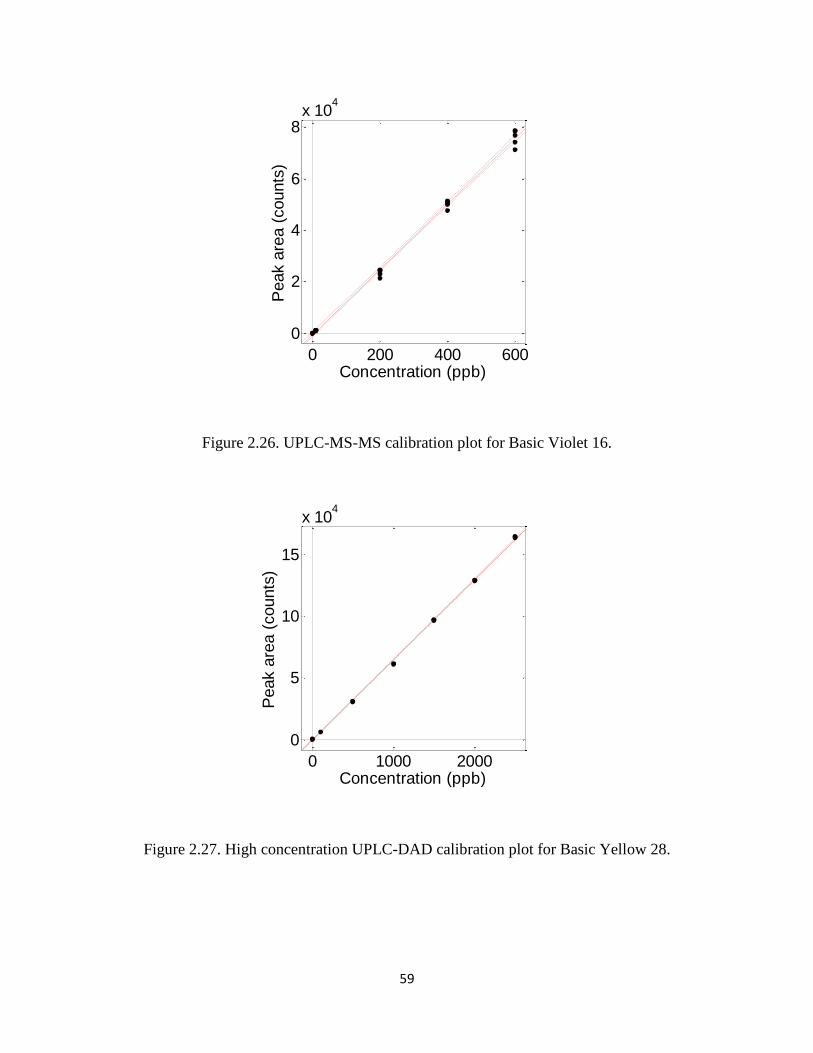
59

Figure 2.26. UPLC-MS-MS calibration plot for Basic Violet 16.

Figure 2.27. High concentration UPLC-DAD calibration plot for Basic Yellow 28.

0 200 400 600

0

2

4

6

8x 10

4

Concentration (ppb)

Peak a

rea (

counts

)

0 1000 2000

0

5

10

15

x 104

Concentration (ppb)

Peak a

rea (

counts

)

60

Figure 2.28. Low concentration UPLC-DAD calibration plot for Basic Yellow 28.

Figure 2.29. UPLC-MS-MS Calibration plot for Basic Yellow 28.

0 20 40

0

500

1000

1500

2000

2500

3000

Concentration (ppb)

Peak a

rea (

counts

)

0 200 400 600

0

2000

4000

6000

8000

Concentration (ppb)

Peak a

rea (

counts

)

61

Figure 2.30. High concentration UPLC-DAD calibration plot for Disperse Blue 60.

Figure 2.31. UPLC-MS-MS Calibration plot for Disperse Blue 60.

0 1000 2000

0

0.5

1

1.5

2

x 104

Concentration (ppb)

Peak a

rea (

counts

)

0 200 400 600

0

2000

4000

6000

8000

10000

Concentration (ppb)

Peak a

rea (

counts

)

62

Figure 2.32. High concentration UPLC-DAD calibration plot for Disperse Violet 77.

Figure 2.33. Low concentration UPLC-DAD calibration plot for Disperse Violet 77.

0 1000 2000

0

5

10

15

x 104

Concentration (ppb)

Peak a

rea (

counts

)

0 20 40

0

500

1000

1500

2000

2500

3000

Concentration (ppb)

Peak a

rea (

counts

)

63

Figure 2.34. UPLC-MS-MS Calibration plot for Disperse Violet 77.

Figure 2.35. High concentration UPLC-DAD calibration plot for Disperse Yellow 114.

0 200 400 600

0

0.5

1

1.5

2

2.5

x 104

Concentration (ppb)

Peak a

rea (

counts

)

0 1000 2000

0

1

2

3

4

x 104

Concentration (ppb)

Peak a

rea (

counts

)

64

Figure 2.36. Low concentration UPLC-DAD calibration plot for Disperse Yellow 114.

Figure 2.37. UPLC-MS-MS calibration plot for Disperse Yellow 114.

0 20 40

0

200

400

600

800

Concentration (ppb)

Peak a

rea (

counts

)

0 200 400 600

0

500

1000

1500

2000

2500

3000

Concentration (ppb)

Peak a

rea (

counts

)

65

CHAPTER THREE

EXTRACTION OF DIRECT AND INDIGO DYES FROM TRACE COTTON FIBERS

FOR FORENSIC CHARACTERIZATION BY ULTRA-PERFORMANCE LIQUID

CHROMATOGRAPHY

66

ABSTRACT

Microextraction, followed by ultra-performance liquid chromatography, can often

distinguish similar fibers containing different, but similar, dyes with the combination of

retention time matching, UV/visible spectral comparison, and structural analysis by mass

spectrometry. The analysis of cotton fibers is challenging because they can be dyed with

three different classes of dye, each requiring a different method for extraction and

analysis. This work focuses on the chemistries of direct dyes and indigo and their

optimum extraction conditions and chromatographic methods. Cotton fibers as small as 1

mm in length have been successfully extracted and characterized. Analytical figures of

merit and validation statistics, including extraction reproducibility, linearity, limits of

detection and quantitation, and UPLC precision, are reported.

INTRODUCTION

The classic example of forensic fiber analysis involves the comparison of "known"

and "questioned" fibers using various microscopic techniques in an attempt to establish

associations between crime scenes, suspects, and victims. Cotton is an extremely

abundant fiber material and cotton fibers are easily identified using polarized light

microscopy by their refractive index and visually based on their unique morphology.1

Additional discriminative information can be obtained from fibers using techniques such

as infrared spectroscopy and UV-visible microspectrophotometry.2 These techniques are

preferred due to them being non-destructive to the fiber sample; however they provide

limited information on the identity and amount of chemical constituents on the fibers.

Though many different types of fibrous textiles are commonly manufactured, 80% of

all fibers found as criminal evidence are made of cotton, nylon, polyester, or acrylic.1–4

67

Cotton is of high interest due to its popularity in clothing. Cotton is a natural fiber made

of cellulose, a polysaccharide containing hydroxyl groups and acetal linkages. The

absence of ionic sites on the polymer backbone necessitates the use of direct dyes that are

attached through hydrogen bonding, and reactive dyes that are covalently bound to the

hydroxyl groups of the polymer. An additional dyeing technique involves water-insoluble

vat dyes which migrate into the cellulose in their reduced form and are then oxidized and

"locked" into the cellulose polymer. Direct, reactive, and vat dyes account for

approximately 82% of all dyes used in the dyeing of cotton.5

Direct dyes are soluble in water due to the abundance of sulfonic acid, amine, and

hydroxyl groups in their structures. The anionic dyes coat the fiber during the dying

process and are held in place through hydrogen bonding. The removal of these dyes

requires the disruption of the hydrogen bonds using alkaline solvents. A 4:3 (v/v) mixture

of pyridine and water has been widely reported to extract direct dyes from cotton

efficiently.6,7

Vat dyes are water-insoluble pigments used to dye cotton and account for

approximately 15-25% of all cotton dyes consumed in the last 20 years.8,9

This usage is

due largely to indigo, an historically important and the oldest discovered vat dye, which

is used today as the primary color of blue jeans. Due to their water-insoluble nature, vat

dyes must first be chemically reduced to their water-soluble leuco form before

application to cotton. Figure 3.1 shows this process for indigo. This process is commonly

referred to as ―vatting‖ in the textile industry as it is usually performed in a large vat.

Vatting is typically conducted using sodium dithionite at very high pH conditions. Once

the leuco form of the dye has been formed, the dye can migrate into the hydrophilic

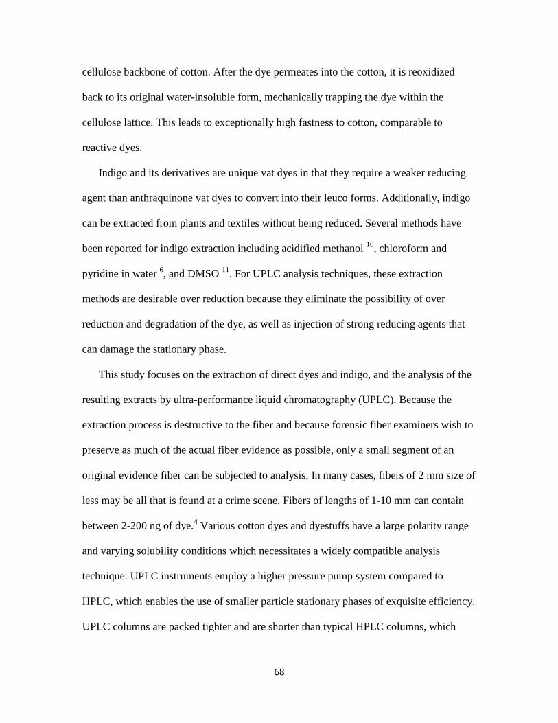
68

cellulose backbone of cotton. After the dye permeates into the cotton, it is reoxidized

back to its original water-insoluble form, mechanically trapping the dye within the

cellulose lattice. This leads to exceptionally high fastness to cotton, comparable to

reactive dyes.

Indigo and its derivatives are unique vat dyes in that they require a weaker reducing

agent than anthraquinone vat dyes to convert into their leuco forms. Additionally, indigo

can be extracted from plants and textiles without being reduced. Several methods have

been reported for indigo extraction including acidified methanol 10

, chloroform and

pyridine in water 6, and DMSO

11. For UPLC analysis techniques, these extraction

methods are desirable over reduction because they eliminate the possibility of over

reduction and degradation of the dye, as well as injection of strong reducing agents that

can damage the stationary phase.

This study focuses on the extraction of direct dyes and indigo, and the analysis of the

resulting extracts by ultra-performance liquid chromatography (UPLC). Because the

extraction process is destructive to the fiber and because forensic fiber examiners wish to

preserve as much of the actual fiber evidence as possible, only a small segment of an

original evidence fiber can be subjected to analysis. In many cases, fibers of 2 mm size of

less may be all that is found at a crime scene. Fibers of lengths of 1-10 mm can contain

between 2-200 ng of dye.4 Various cotton dyes and dyestuffs have a large polarity range

and varying solubility conditions which necessitates a widely compatible analysis

technique. UPLC instruments employ a higher pressure pump system compared to

HPLC, which enables the use of smaller particle stationary phases of exquisite efficiency.

UPLC columns are packed tighter and are shorter than typical HPLC columns, which

69

allows for significantly faster chromatographic analyses, sharper peaks, and higher

signal-to-noise measurements. As in other forms of liquid chromatography, both the

column and mobile phase systems can be tuned to analyze samples of varying chemical

makeup.

EXPERIMENTAL

Materials and Instrumentation

Analytical grade water, acetone, pyridine, ammonium acetate, dimethyl sulfoxide

(DMSO), chloroform, formic acid, glacial acetic acid, and HPLC/UPLC grade

acetonitrile and methanol were purchased from Fisher Scientific (Pittsburg, PA).

Dye standards and extracts were separated and detected using a Waters Acquity™

UPLC H-Class equipped with a quaternary solvent pump system and a Waters PDA e

detector. The column was a 2.1 50 mm I.D. 1.7 m particle size Waters Acquity™

BEH C18 column with a 2.1 5 mm I.D. 1.7 m particle size Waters Acquity UPLC

BEH C18 VanGuard precolumn. Mobile phase gradients are shown in Table 3.3 and

Table 3.4. The column temperature was set at 40 °C. The diode array detector scanned at

a rate of 40 Hz and 1.2 nm resolution. The sample injection volumes were 10 L.

All dyed fabrics and matching dye standards were current production samples

donated by dyestuff manufacturers in the southeastern United States. Dye names follow

the Color Index nomenclature. All fibers were dyed at levels consistent with commercial

use (2–4% by weight). All dye standards were solid in phase and stored in a dark room to

avoid photodegradation. Photographs of cotton fibers were made with a Nikon (Melville,

NY) model SMZ1500 microscope with a DS-Fi1 camera at 11.25x magnification.

Direct Dye Extraction Optimization

70

Direct Blue 71 (structure in Table 3.1) was selected as a representative direct dye for

cotton fibers. Fibers dyed with this single dye were extracted under the solvent

combinations shown in Table 3.2, generated using a three-component mixture design

with Design Expert 7 (Milwaukee, WI). For each of the ten design points, four replicate 1

cm threads dyed with Direct Blue 71 were individually subjected to microextraction.

Extractions at each design point were performed on four replicate fibers of the same

length, for a total of 40 extractions. Extractions were conducted in Waters Total

Recovery Vials because the narrow diameter of the vial allows the entire fiber sample to

be submerged in less solvent than that of a typical conical vial, concentrating the extract.

The threads were extracted by adding 1 mL of solvent, capped, and heated in an oven at

100°C for 60 min. Following extraction, the vials were uncapped and the solvents were

evaporated at 95°C and then reconstituted in 1 mL of water for UPLC analysis. A Waters

(Milford, MA) Acquity H-Class Quaternary Solvent UPLC coupled to a Waters PDA e

diode array detector for UV-visible analysis and equipped with a Waters Acquity BEH

C18 column (1.7 um particle size, 2.1 mm ID x 50 mm length) was used for all analysis.

The diode array detector measured absorbance from 400-700 nm at 40 Hz and 1.2 nm

resolution. Dye peak areas were used as the response, and ternary response surface

models were generated using Design Expert, v. 7 (StatEase Corp., Inc., Minneapolis,

MN, USA). The mobile phase gradient conditions are given in Table 3.3.

Indigo Dye Extraction Optimization

A second ternary component mixture containing chloroform, pyridine, and DMSO

was studied for the extraction of indigo. As with the direct dye optimization study, five

replicate fibers were extracted at each design point and then quantified by UPLC. The

71

solvents used were DMSO, chloroform, and pyridine. Extractions were carried out at

100°C for 60 min in 1 mL of solvent. The solvent was then boiled off and samples were

reconstituted in 1 mL of 50:50 methanol and water. UPLC gradient conditions for indigo

analysis are listed in Table 3.4.

Limits of Detection and Extract Quantitation

Standard mixtures of direct dyes were made 1-10 ppm concentrations. The direct dye

mixtures contained Direct Blue 80, Direct Blue 71, and Direct Orange 39 in 90:10 (v/v)

0.2 M ammonium acetate and acetonitrile. The dye mixtures were analyzed (five

replicates) using UPLC. A calibration plot was generated for each dye and limits of

detection were determined.

Direct Dye Extraction

For the extraction of direct dyes, fibers 1 cm in length, dyed with Direct Orange 39,

Direct Blue 71, or Direct Blue 80 from Dystar (structures shown in Table 3.1), were cut

using a fiber guillotine and loaded into total recovery vials. 100 μL of optimal extraction

solvent mixture (50% DI H2O, 25% pyridine, 25% Acetone) was dispensed into the vial.

The vials were sealed with screw tops to minimize solvent evaporation and were placed

in a laboratory oven at 100°C for 60 min. The vials were uncapped and allowed to

completely evaporate in the oven at 95°C. Dye residues were reconstituted with 50 uL

90% 0.2 M ammonium acetate and 10% acetonitrile and vortex-mixed to ensure

solvation. The dyes were then analyzed by UPLC-DAD using the same chromatographic

conditions as the extraction study.

72

Indigo Extraction

It was determined from the indigo extraction optimization that the optimum

extraction solvent was 100% DMSO. Extractions were carried out by adding 100 μL of

DMSO to the fibers in the vials which were then capped and heated to 100°C for 60 min.

After extraction, the extractant was allowed to cool to room temperature and then

injected.

Dye samples were analyzed using a diode array detector measuring absorbance from

400-700 nm. The area of the peak on the chromatogram was acquired for each dye using

the corresponding maximum wavelength (for Direct Orange 39, Direct Blue 80, and

Direct Blue 71 at 420, 571, and 586 nm, respectively), and compared to standard

mixtures of dyes to quantify the amount of dye on each fiber.

RESULTS AND DISCUSSION

Extraction optimization for direct dyes

Figure 3.2 displays a three dimensional fitted surface and contour plot for the

absorbance of direct dye extracts as a function of solvent conditions. Optimum

absorbance is predicted at 51.5% A (water), 20.6% B (pyridine), and 27.9% C (acetone).

Because the region around this optimum is relatively flat, this outcome is relatively

robust: slight variations in solvent conditions do not diminish significantly the amount of

dye extracted. For ease of use, 50% water, 25% pyridine, and 25% acetone was employed

for direct dye extractions.

Table 3.5 shows variability of UPLC peak retention and area for extracts of Direct

Blue 80 for ten replicate dyed cotton fibers taken from the same 1 cm thread Variability

in amounts of dye extracted from single fibers originates from several sources. The Q test

73

rejected the data from Fiber 4 as an outlier at the 99% level of confidence. The percent

relative standard deviation (%RSD) for the fiber extractions, if the datum from Fiber 4 is

retained, was 47.4%.; after deleting the outlier, the RSD drops to 35.4%. These results are

typical for cotton. Unlike synthetic fibers (e.g., nylon), natural cotton fibers exhibit

biological variety and differ in morphology among fibers and even along the length of the

same fiber. Physical parameters that may differ include diameter, cross section shape,

degree of fiber convolutions, and surface area. Many of these characteristics are affected

by the processes to which cotton is subjected prior to dyeing, such as desizing, bleaching,

or mercerization. Although mercerization (treatment with sodium hydroxide) commonly

makes cotton cross section more rounded and decreases convolutions, process variations

may impart variations in fiber shape.12

Figure 3.3 shows an optical microscopy photograph of several cotton fibers. Because

cotton fiber morphology exhibits variability, dye amounts on an individual fiber can vary

significantly from the other 80-100 fibers taken from the same segment of thread.

Additionally, fibers on the inside of the thread can also be "shielded" by those on the

outside during the dyeing process, also affecting dye uptake.

Extraction optimization for indigo

Design Expert 8 (Statease Corp., Minneapolis, MN) was used for construction of

experimental designs and response surface modeling. Figure 3.4 shows the fitted

response surface for the indigo extraction optimization study. The calculated model-F

value indicated that a linear model best fit the data. According to the model, the optimum

extraction solvent mixture is pure DMSO. This result is favorable because mixtures of

DMSO, chloroform, and pyridine when heated evolved pungent fumes that smelled

74

characteristic of hydrogen sulfide. DMSO is also compatible with C18 stationary phase,

thus the reconstitution step after dye extraction can be skipped and the extract injected

after cooling to room temperature, minimizing potential sample loss during evaporation.

UPLC of dye standards

Separation of the direct dye standards shows that some of the dyes have multiple

components. In Figure 3.5, Direct Orange 39 is clearly comprised of two dye

components. Many smaller peaks are also obvious in the expanded view of Figure 3.6.

These peaks can be attributed to various "dyestuffs" that are added during the dyeing

process such as compounds that aid in the dye-uptake by the fibers, finishing agents, and

fluorescent brighteners. Indigo did not contain any miscellaneous peaks and its

chromatogram is shown in Figure 3.7. UV/visible spectra for the main dye peaks are

shown in Table 3.1.

Limit of Detection

The limits of detection and quantification for each dye can be determined from the

calibration models by:

LOD = 3.3σb/S

LOQ = 10σb/S

where σb is the standard deviation of the blank and S is the slope of the calibration model.

LOD and LOQ values are reported in Table 3.6 using three different methods that differ

in how σb is estimated. LOD1and LOQ1 estimate σb using the standard deviation of the

integrated noise signal across the width of the actual peak. LOD2 and LOQ2 estimate σb

by calculating the standard deviation of the lowest concentration calibrator and requires

this concentration to be near the actual LOD to be considered accurate. LOD3 and LOQ3

75

estimate σb using the standard deviation of the y-intercept of the calibration line. Variance

in the high concentration calibrators will increase the variance of the y-intercept leading

LOD3 to provide a high estimate for LOD and LOQ.

Calibration models had generally good fit with coefficients of determination of

0.9997 for Direct Orange 39 and Direct Blue 71, 0.9946 for Direct Blue 80, and 0.9986

for Indigo. The calibration plot for Direct Blue 80 is shown in Figure 3.8. Detection

limits were below 1 ppb for three of the dyes according to LOD1 due to low and

reproducible noise. LOD2 showed values in the 25-60 ppb range for the direct dyes and

6.07 ppb for Indigo. LOD2 for Indigo is lower due to the addition of a 500 ppb calibrator

not present for the direct dyes. Direct Blue 80 has the lowest LOD2 value despite having

higher LOD1 and LOD3 values because it has the lowest detector response of all the dyes,

resulting in a lower standard deviation for the lowest calibrator. The LOD3 values are the

highest overall due to the number of high concentration calibrators. Variance in the high

concentration region of a calibration model can lead to high variance of the y-intercept.

Together, LOD1, LOD2, and LOD3 present a possible range for the true limit of detection

to reside. With exception to LOD3, all calculated detection limits indicate that detection

of 2 ng of dye from a 1 mm fiber is possible.

Trace fiber extractions

Direct dyes were extracted and detected from fibers of lengths down to 1 mm.

Because of their non-uniform morphology, cotton fibers do not lay flat. Cutting cotton

fibers reproducibly to small lengths is difficult. We found that cutting an entire thread to

the desired length and then unweaving the fibers from that thread produced many fibers

of lengths very close to the desired length. These fibers can then be examined under a

76

magnifying glass using a ruler and similar length fibers can be selected. As fiber length

decreases down to 1 mm, handling of the fibers becomes extremely difficult. It is very

important to ensure that the fiber is deposited on the bottom of the inside of the vial, and

that extractant covers the entire fiber. Additionally, during the extractant evaporation

stage, care must be taken to not let the extractant boil. Otherwise extracted dye will be

deposited all over the inside of the vial and lower the amount that is successfully

reconstituted.

A batch of three 1 mm fibers that were cut from a thread dyed with Direct Blue 71

were analyzed. Of the three samples, only one was extracted successfully. This was due

entirely to the difficulty of handling 1 mm fibers. The chromatogram for the 1 mm fiber

extract is shown in Figure 3.9. The dye peak is located at 1.85 min. The RMS signal-to-

noise for the dye peak of interest is 118.05. The negative response and sloping baseline is

due to the mobile phase gradient response on the UV/visible detector.

Another extraction study was conducted on 5 mm fibers to compare their extraction

success to the 1 mm extraction study. Five samples were taken from the same 5 mm

thread and similar length fibers were chosen for extraction. Of the five samples, four

were extracted successfully and the data is presented in Table 3.7. The %RSD for the

four successful 5 mm extractions was 38.73% and is comparable to the 35.42% RSD for

the 1 cm reproducibility study.

Indigo was successfully extracted from a 1 mm fiber and detected by UPLC-DAD. A

set of five 1 mm indigo-dyed cotton fibers were extracted using DMSO. Because DMSO

has such a high boiling point and is compatible with the C18 stationary phase, the boil-off

and reconstitute step of the extraction process was skipped, and the extract was injected

77

directly into the UPLC after cooling to room temperature. The extract chromatogram had

a RMS signal-to-noise of 62.80 and is shown in Figure 3.10.

CONCLUSIONS

Solvent conditions were optimized for the extraction of direct and indigo dyes from

cotton. UPLC separation methods were also devised that, together with the optimized

extraction conditions, was successful in detecting extracts from single 1 mm length fibers

with RMS signal-to-noise ratios of 118.05 and 62.80 for Direct Blue 71 and Indigo

respectively. Calibration models yielded limits of detection and quantification as low as

2.1pg and 6.2 pg respectively, suggesting the possibility of analyzing sub-millimeter

length fibers. Handling fibers of millimeter and sub-millimeter lengths continues to be a

challenge and new fiber handling techniques need to be developed. Future work will

involve mass spectrometry characterization of the various dye stuffs present in the dye

standards as well as characterizing finishing agents from fiber extracts.

ACKNOWLEDGMENTS

Coauthors of this work include Molly R. Burnip, Kaylee R. McDonald, and Stephen

L. Morgan (Department of Chemistry and Biochemistry, University of South Carolina,

Columbia, SC 29208). Research in this presentation was supported by award 2010-DN-

BX-K245 from the National Institute of Justice, Office of Justice Programs, U. S.

Department of Justice. The opinions, findings, and conclusions or recommendations

expressed in this publication are those of the author(s) and do not necessarily reflect those

of the Department of Justice. Mention of commercial products does not imply

endorsement on the part of the National Institute of Justice or the University of South

Carolina.

78

References

(1) Robertson, J.; Grieve, M. Forensic Examination of Fibres; 2nd ed.; Taylor &

Francis: London, 1999.

(2) Rendle, D. F.; Wiggins, K. G. Forensic analysis of textile fibre dyes. Review of

Progress in Coloration and Related Topics 1995, 25, 29–34.

(3) Gaudette, B. D. The forensic aspects of textile fiber examination. Chapter 5 in:

Forensic Science Handbook, vol. 2, R. Saferstein, Ed.; Prentice Hall: Englewood

Cliffs, NJ, 1988.

(4) Macrae, R.; Smalldon, K. The Extraction of Dyestuffs from Single Wool Fibers. J.

Forensic Sci. 1979, 24, 109–116.

(5) Shore, J.; Colourists, S. of D. and Colorants and Auxiliaries: Colorants; Society of

Dyers and Colourists, 2002.

(6) Laing, D.; Dudley, R.; Hartshorn, A.; Home, J.; Rickard, R.; Bennet, D. The

extraction and classification of dyes from cotton and viscose fibres. Forensic

Sci.Int. 1991, 50, 23–35.

(7) Cheng, J.; Wanogho, S. O.; Watson, N. D.; Caddy, B. The extraction and

classification of dyes from cotton fibres using different solvent systems. J.

Forensic Sci. Soc. 1991, 31, 31–40.

(8) Meksi, N.; Ben Ticha, M.; Kechida, M.; Mhenni, M. F. Using of ecofriendly α-

hydroxycarbonyls as reducing agents to replace sodium dithionite in indigo dyeing

processes. Journal of Cleaner Production 2012, 24, 149–158.

(9) Hunger, K. Industrial dyes: Chemistry, Properties, Applications; Wiley-VCH,

2003.

(10) Surowiec, I.; Quye, A.; Trojanowicz, M. Liquid chromatography determination of

natural dyes in extracts from historical Scottish textiles excavated from peat bogs.

J. Chromatogr. A 2006, 1112, 209–17.

(11) Michel, R. H.; Lazar, J.; McGovern, P. E. The chemical composition of the

indigoid dyes derived from the hypobranchial glandular secretions of Murex

molluscs. Journal of the Society of Dyers and Colourists 1992, 108, 145–150.

(12) Incorporated, C.; Staff, C. I. Cotton Dyeing and Finishing: A Technical Guide;

Cotton, Incorporated, 1997.

79

Table 3.1. Structures and spectra of the direct dyes and indigo.

Structure Absorbance Spectra

400 500 600

5000

10000

15000

Wavelength (nm)

Absorb

ance (

mA

U)

400 500 600

1

2

3

4

5

6

7

x 104

Wavelength (nm)A

bsorb

ance (

mA

U)

400 500 600

0.5

1

1.5

2

2.5

x 104

Wavelength (nm)

Absorb

ance (

mA

U)

300 400 500 600 700

0.5

1

1.5

2

x 106

Wavelength (nm)

Absorb

ance (

mA

U)

80

Table 3.2. Solvent compositions for each design point for the extraction optimization for

direct-dyed cotton fibers.

Design

Point

A: Water

(%)

B: Pyridine

(%)

C: Acetone

(%)

1 100 0 0

2 0 100 0

3 0 0 100

4 50 50 0

5 50 0 50

6 0 50 50

7 33.33 33.33 33.33

8 66.66 16.66 16.66

9 16.66 66.66 16.66

10 16.66 16.66 66.66

81

Table 3.3. Mobile phase conditions for the analysis of direct dyes by UPLC.

Time

(min)

Flow Rate

(mL/min)

%

Methanol

% 0.2 M

Ammonium

Acetate

%

Acetonitrile

Initial 0.45 5 90 5

5 0.45 5 5 90

6 0.45 5 90 5

8 0.45 5 90 5

82

Table 3.4. Mobile phase conditions for the analysis of indigo by UPLC.

Time

(min)

Flow

Rate

(mL/min)

% Water

(0.15%

Formic

Acid)

%

Methanol

0 0.5 70 30

0.25 0.5 70 30

2 0.5 0 100

3 0.5 0 100

3.1 0.5 70 30

5.5 0.5 70 30

83

Table 3.5. Peak retention time and area reproducibility for 1 cm fibers dyed with Direct

Blue 80.

Fiber Retention

time (min) Area (counts)

1 1.34 28667.68

2 1.35 14122.29

3 1.34 25609.83

4 1.33 68574.72

5 1.34 34615.79

6 1.34 21941.95

7 1.34 37175.18

8 1.33 49014.68

9 1.34 33480.44

10 1.34 20549.12

84

Table 3.6. Limits of detection and quantitation of the direct and indigo dyes. Calculations

based on the standard deviation of the blanks (LOD/LOQ1), the standard deviation of the

lowest concentration calibrator (LOD/LOQ2), and the standard deviation of the y-

intercept of the calibration plot (LOD/LOQ3).

Dye R2

LOD1

(ppb)

LOD2

(ppb)

LOD3

(ppb)

LOQ1

(ppb)

LOQ2

(ppb)

LOQ3

(ppb)

Direct Blue 80 0.9946 1.39 26.3 166 4.21 79.7 503.03

Direct Orange 39 0.9997 0.83 59.3 39.6 2.5 179.7 120

Direct Blue 71 0.9997 0.21 44.2 39.5 0.63 133.94 119.7

Indigo 0.9986 0.74 6.07 79.9 2.23 18.39 242.12

85

Table 3.7. Peak areas for four 5 mm fiber extracts for Direct Blue 71.

Fiber Peak Area

1

19319.44

2

25204.23

3

28823.84

4

10275.35

%RSD

38.73

86

Figure 3.1. Reduction of indigo to its water-soluble leuco form.

87

Figure 3.2. Perspective view (left) and contour plot (right) of fitted absorbance response

surface for direct dye extraction as a function of solvent conditions. Design points from

Table 3.2 are indicated by solid dots. A, Water; B, Pyridine; C, Acetone.

88

Figure 3.3. Optical microscope image (magnification12.5) of cotton fibers

dyed with Direct Orange 39.

89

Figure 3.4. Fitted linear absorbance response surface for Indigo extraction as a function

of solvent conditions Design points follow those from Table 4.2 and are indicated by

solid dots. A, DMSO; B, Chloroform; C, Pyridine.

90

Figure 3.5. Chromatogram showing the separation of all three direct dyes. Some dyes

have multiple components. Peak 1 is Direct Blue 80, peak 2 is Direct Blue 71, and peak 3

is Direct Orange 39.

0.5 1 1.5 2 2.5 30

2

4

6

8

10

12

14x 10

6

Retention time (min)

Absorb

ance (

counts

)

1

2

3

91

Figure 3.6. Multiple direct dye component in the chromatographic region of 1 to 2,5 min

from Figure 3.5. Peak 1 is Direct Blue 80, peak 2 is Direct Blue 71, peak 3 is Direct

Orange 39, and peaks labeled ―D‖ are miscellaneous dye stuff.

1 1.5 2 2.5

0

2

4

6

x 105

Retention time (min)

Absorb

ance (

counts

)1

2 3 1

D

D

D D D

D

3

92

Figure 3.7. UPLC-DAD chromatogram of Indigo.

0.5 1 1.5 2 2.50

1

2

3

4

5

6

x 107

Retention time (min)

Absorb

ance (

counts

)

93

Figure 3.8. Calibration relationship for Direct Blue 80.

0 5 10

0

2

4

6

8

10

x 104

Concentration (ppm)

Peak a

rea (

counts

)

94

Figure 3.9. Chromatogram of 1 mm Direct Blue 71 dye peak from 1.6-2 min.

95

Figure 3.10. Chromatogram of the extraction of Indigo from a 1 mm cotton fiber.

1.44 1.46 1.48 1.5 1.52 1.54-4

-3.5

-3

-2.5

-2x 10

5

Retention time (min)

Absorb

ance (

counts

)

96

CHAPTER FOUR

EXTRACTION AND CHARACTERIZATION OF REACTIVE DYES AND THEIR

HYDROLYSIS PRODUCTS FROM TRACE COTTON FIBERS BY ULTRA-

PERFORMANCE LIQUID CHROMATOGRAPHY

97

ABSTRACT

Microextraction and ultra-performance liquid chromatography methods have been

developed for reactive dyes on cotton. Reactive dyes are chemically bound to the

cellulose structure of the fiber and present an analytical challenge to the forensic fiber

examiner because release of these dyes requires breaking of the covalent bond using hot

sodium hydroxide. The resulting hydrolysis reactions can also cleave amide bonds and

possibly other chemical bonds in the dye molecule. The various structural changes that

can take place leads, in many cases, to production of multiple reaction products from a

single dye molecule. We demonstrate successful extraction of reactive dyes from single 1

mm cotton fibers with detection limits as low as 3.3 pg. Systematic experiments at

varying reaction conditions, with product analysis by mass spectrometry, were also

performed to characterize the degradation of reactive dyes under hydrolysis, and to

facilitate interpretation of reactive dye extractions.

INTRODUCTION

Cotton fibers are unique in the textile industry because they can be dyed with three

different classes of dyes: direct, vat, and reactive. Reactive dyes differ from most other

dye classes in that they are covalently bound to the fiber. This makes reactive dyes the

most substantive of dyes used on cotton because the covalent bonding of the dye to the

fiber provides excellent fastness to laundering. As a result, reactive dyes are the most

popular dye class used to color cotton textiles. Figure 4.1 summarizes worldwide

consumption of cotton dyes in 2003, showing that reactive dyes constitute 50% of all

dyes on cotton textiles.1

98

The reactive dyeing process typically involves the reaction of a haloheterocycle such

as a chlorotriazine on the dye with a hydroxyl group on the fiber.2,3

Reactive dyes can

also attach to cotton via vinylsulphone groups that form activated alkenes when treated

with sodium hydroxide, as shown in Figure 4.2. The extraction of reactive dyes from

cotton requires the hydrolysis of the covalent bond using sodium hydroxide at elevated

temperatures via the mechanism shown in Figure 3.5

This study focuses on the extraction of reactive dyes from cotton followed by

separation and detection using ultra-performance liquid chromatography (UPLC). This

chemical extraction process is destructive to the fiber and the dyes itself because sodium

hydroxide and heat are used to break the covalent fiber-dye bond. Our research

hypothesis is that, despite chemical degradation of the original dye to various products,

separation of the resulting product mixture and (ultimately, identification of components

by mass spectrometry) can provide forensic profiling to discriminate reactive dyes from

one another. Improved understanding of reactive dye degradation can also assist

interpretation of extracted components and potentially enable identification of the parent

reactive dye. Trace evidence fibers can often be as short as 10 mm and contain between

2-200 ng of dye.6 Emphasis will be placed on optimizing extraction and UPLC conditions

to facilitate extracting from 1 mm fibers.

EXPERIMENTAL

Analytical grade water, sodium hydroxide, ammonium acetate, ammonium

hydroxide, and HPLC/UPLC grade acetonitrile were purchased from Fisher Scientific

(Pittsburg, PA).

99

Dyed fabrics and matching dyes standards were current production samples donated

by dyestuff manufacturers in the southeastern United States. Dye names reported here

follow the Color Index nomenclature (Society of Dyers and Colourists, Bradford, UK).

All fibers were dyed at levels consistent with commercial use (2–4% by weight). All dye

standards were solid in phase and stored in a dark room to avoid photodegradation.

Literature has suggested that 1.5% NaOH and heat should be used to facilitate the

extraction of reactive dyes from cotton.6-9

Previous reactive dye extraction work in our

laboratory has also employed these conditions.2 Hydrolysis presents a number of

potential issues. The dye to be extracted may change its chemical form under hydrolysis

conditions. Strongly alkaline solutions are also not compatible with many stationary

phases for liquid chromatography. In the present work, reactive dye standards were

treated with 1.5% sodium hydroxide and heated at 100 °C for 60 min. The resulting

solution was then treated with equimolar hydrochloric acid to neutralize any excess

sodium hydroxide remaining prior to liquid chromatography.

Fibers of lengths 10 mm, 5 mm, and 1 mm dyed with Reactive Yellow 160, Reactive

Blue 220, or Reactive Orange 72 (structures shown in Table 4.1) were cut with a fiber

guillotine (as described in chapter 2) and placed into 200 µL conical Total Recovery

Vials. A 50 μL aliquot of 0.1875 M sodium hydroxide was dispensed into the vial and

sealed to prevent evaporation. Extraction was carried out in the laboratory oven at 100°C

for 60 min. The dyes were reconstituted by addition in sequence of 25 µL of 0.375 M

hydrochloric acid (equimolar with the sodium hydroxide), 25 μL of 10 mM ammonium

acetate adjusted to pH 9.3. Dyes were separated using a Waters Acquity UPLC system

coupled to a diode array detector (DAD). The system was equipped with a room

100

temperature sample manager and a Waters Acquity BEH C18 column (1.7 um particle

size, 2.1 mm ID × 50 mm length) heated to 40 °C. The mobile phase solvent gradient

conditions employed for all runs is listed in Table 4.2. The sample injection volumes

were 10 L.

Dyes samples were detected using a UV/visible diode array detector scanning

absorbance from 300-700 nm. The peak area on the chromatogram was acquired for each

dye using the corresponding maximum wavelength (for Reactive Yellow 160, Reactive

Blue 220, and Reactive Orange 72 at 405 nm, 610 nm, and 478 nm, respectively), and

was used for comparison to standard dye mixtures to determine the amount of dye on

each fiber.

Limits of detection and quantitation were determined from calibration models based

on the UPLC-DAD analysis of reactive dye standards at varying concentrations.

Calibration solutions were made for each dye in water at concentrations 100 ppb, 200

ppb, 400 ppb, 600 ppb, 800 ppb, and 1000 ppb. Five replicates samples were prepared at

each concentration level and analyzed by UPLC-DAD.

RESULTS AND DISCUSSION

A chromatogram showing the separation of the mixture of three reactive dyes is

shown in Figure 4.4. Figure 4.5 shows a magnified view of the retention time window for

0.75 to 2.75 min within which multiple additional components are present. As indicated,

most of these peaks have UV/visible absorbance spectra that match those of the one of

three primary reactive dyes. We initially assumed that these peaks are secondary

degradation products derived from the corresponding primary dyes, or represent other

contaminants introduced during the dye manufacturing process. UV/visible absorbance

101

spectra of the main dye peaks are shown in Table 4.1. During method development, the

first eluting peak, Reactive Blue 220, displayed poor chromatographic peak shape and

lower peak height than the other dyes. The addition of 10 mm ammonium acetate

adjusted to pH 9.3 resulted in sharpening this peak.

UPLC-DAD analysis of extracted reactive dyes

UPLC-DAD analysis of reactive dyes treated with 1.5% NaOH confirmed that

additional reactions occur during the extraction process. Figure 4.6 shows the

chromatograms for Reactive Orange 72 standard and ―extracted‖ (treated with NaOH).

The standard chromatogram shows a single peak corresponding to the dye with an

absorbance maximum of 478 nm. The extracted chromatogram shows two peaks, both of

which increased in retention, and the main peak having an absorbance maximum of 473

nm. Because the second peak showed a similar absorbance maximum, we hypothesized

that both peaks were ―dye‖ and that one of the peaks was due to the incomplete base-

hydrolysis of the dye standard.

To test this hypothesis, a nominal starting ratio of NaOH to dye was first established.

Assuming that a single 1 cm cotton fiber contained 20 ng of dye, using 50 μL of 1.5%

NaOH to extract the dye from the fiber gives a ratio of 9.375 × 10-7

moles of NaOH to 1

ng of dye. For the purposes of later comparisons, other ratios were expressed as a

percentage of this value. Several 1 ppm standards of Reactive Orange 72 were then

treated with amounts of NaOH varying 10%-150% of that amount, neutralized with

equimolar HCl, and analyzed by UPLC-DAD. Figure 4.7 displays the dependence of the

resulting peak areas peaks on NaOH amount. Approximately 50% of the nominal amount

of NaOH is required to completely hydrolyze the dye molecule. Due to the variability of

102

the amount of dye on cotton fibers, 75% of the nominal amount was selected as a

compromise between ensuring complete extraction and hydrolysis of the dye and

maintaining a low amount of NaOH in solution. Thus, a 1 cm length of a single cotton

fiber requires 50 µL of 0.28125 M NaOH for the extraction of a reactive dyes. The

amount of NaOH can then be adjusted depending on the length of the cotton fiber of

interest.

HPLC-MS of reactive dyes

HPLC-MS confirms that reactive dyes undergo additional reactions during NaOH

extraction from cotton. Both C. I. Reactive Orange 72 and Reactive Yellow 160 were

analyzed using negative-ion electrospray ionization (ESI-) mass spectrometry. C. I.

Reactive Blue 220 did not did not appear in HPLC-MS due to the requirements of using

an acidic buffer for the MS analysis (basic buffer is required to maintain a proper

chromatographic peak shape for Reactive Blue 220).

Analysis of the C. I. Reactive Yellow 160 standard by HPLC-MS shows at least four

derivatives of the dye molecule (Figure 4.8). The molecular mass of Reactive Yellow 160

is 653 g/mol and elutes at a retention time of 16.61 min with a characteristic ion of m/z

652 due to deprotonation of the dye in solution. Derivatives of this molecule appearing at

m/z 572 and 554 are probably due to the loss of a sulfonic acid and a sulfate functional

group, respectively. The longer retention time for these products can be attributed to the

decrease in their mobile phase solubility on losing these functional groups, and their

increased affinity for the non-polar C18 stationary phase. Additional fragments of mass

m/z 572 m/z and 554 appear in the mass spectra of Reactive Yellow 160 peak at 16.61

min. The structure of the component of m/z 614 is unknown, however it has an almost

103

identical absorbance spectra to that of the dye molecule and its other derivatives (Figure

4.9), suggesting that it also is a derivative of the dye.

Treatment of Reactive Yellow 160 dye standard with NaOH to simulate the extraction

conditions yielded two products observable by HPLC-MS (ESI-), as shown in Figure

4.10. The combination of NaOH and heat (100°C) hydrolyzes the amide bond and

removes the sulfate group, as seen in the second product at 18.66 min. This compound

fragments further with the cleavage of the azo group. Because this compound is a beta-

keto acid, it undergoes decarboxylation under basic conditions and heat, with loss of

carbon dioxide, resulting in the product eluting at 15.07 min.

Analysis of the Reactive Orange 72 dye standard by HPLC-MS also shows multiple

derivatives of the dye. The total ion chromatogram shows only a single chromatographic

peak with a mass spectrum containing a spectral peak at 474 m/z, as seen in Figure 4.11.

This result is unexpected because the reported mass for Reactive Orange 72 is 572 g/mol.

Isolation of 572 m/z from the chromatogram yields a broad chromatographic peak, and

the combined spectra for this peak shows what appears at first glance to be a

fragmentation pattern for the dye molecule. However, ESI should not yield much, if any,

fragmentation as it is a ―soft‖ ionization technique. Extraction of the prominent masses

572 m/z, 492 m/z, 474 m/z, and 417 m/z from the TIC yields four separated

chromatographic peaks, shown in Figure 4.12, suggesting that our Reactive Orange 72

dye standard is actually a mixture of multiple compounds. The combination of this result

for Reactive Orange 72with the multiple derivatives of Reactive Yellow 160 suggests

mixtures of multiple compounds may be common for all reactive dyes.

104

Reactive Orange 72 was also treated with NaOH to simulate an extraction. The

resulting chromatogram, shown in Figure 4.13, as expected only contained one peak of

interest. Unlike Reactive Yellow 160, Reactive Orange 72 has an ―external‖ amide bond

which upon hydrolysis leaves the bulk of the dye molecule unchanged.

Limits of Detection

The limits of detection and quantification for each dye can be determined from the

calibration models by:

LOD = 3.3σb/S

LOQ = 10σb/S

where σb is the standard deviation of the blank and S is the slope of the calibration model.

LOD and LOQ values are reported in Table 4.6 using three different methods that differ

in how σb is estimated. LOD1and LOQ1 estimate σb using the standard deviation of the

integrated noise signal across the width of the actual peak. LOD2 and LOQ2 estimate σb

by calculating the standard deviation of the lowest concentration calibrator and requires

this concentration to be near the actual LOD to be considered accurate. LOD3 and LOQ3

estimate σb using the standard deviation of the y-intercept of the calibration line. Variance

in the high concentration calibrators will increase the variance of the y-intercept leading

LOD3 to provide a high estimate for LOD and LOQ.

The calibration models produced high coefficients of determination of 0.9987 for

Reactive Yellow 160, 0.9989 for Reactive Blue 220, and 0.9993 for Reactive Orange 72.

All three LOD estimates yield detection limits in the 3 pg to 83 pg range (based 10 L

injections) which is low enough to detect extracts from 1 mm fibers. LOQ values range

105

from 10 pg and 252 pg and suggests the possibility of conducting quantitative

comparisons between 1 mm fiber extracts.

Trace fiber extractions

All three reactive dyes were extracted and detected from fibers of lengths down to 1

mm. Because of their non-uniform morphology, cotton fibers do not lay flat. Cutting

cotton fibers reproducibly to small lengths is difficult. As fiber length decreases down to

1 mm, handling of the fibers becomes extremely difficult. The reactive extractions

showed the same amount of variance in the amount extracted from equal length fibers

from the same thread. This variance is explained by the biological nature of cotton which

produces fibers of different diameters and shapes capable of containing different amounts

of dye. Analysis of this variability was conducted in Chapter 3. Figure 4.17 shows

successful extraction and detection of a 10 mm, 5 mm, and 1 mm cotton fiber dyed with

Reactive Yellow 160. Close inspection of the 1 mm extraction chromatogram suggests

that 1 mm fibers dyed with Reactive Yellow 160 are near the fiber length limit of this

method. The calibration model for Reactive Yellow 160 returns concentrations of 135

ppb, 35 ppb, and 12 ppb for the 10 mm, 5 mm, and 1 mm extractions respectively.

Comparing these values to those in Table 4.3 confirms that the 1 mm extract of Reactive

Yellow 160 is detected and is arguably quantifiable.

CONCLUSIONS

Methods for the extraction of reactive dyes from cotton using sodium hydroxide have

been reported. Extraction using hot sodium hydroxide results in hydrolysis of the dye-

cellulose bond as well as hydrolysis of the amide bonds in the dye molecule. The reported

UPLC-DAD method gave detection limits as low as 0.33-1.42 ppb and quantitation limits

106

as low as 1.00-4.30 ppb, and detection and quantification of 1-10 mm extracts of

Reactive Yellow 160 were confirmed. Future work on this project will require the

construction of calibration models based on the simulated extraction of the dye standards

by addition of sodium hydroxide and heat. Additional extractions are also needed to

solidify the validity of the method.

ACKNOWLEDGMENTS

Coauthors of this work include Molly R. Burnip and Stephen L. Morgan (Department

of Chemistry and Biochemistry, University of South Carolina, Columbia, SC 29208).

Research in this presentation was supported by award 2010-DN-BX-K245 from the

National Institute of Justice, Office of Justice Programs, U. S. Department of Justice. The

opinions, findings, and conclusions or recommendations expressed in this publication are

those of the author(s) and do not necessarily reflect those of the Department of Justice.

Mention of commercial products does not imply endorsement on the part of the National

Institute of Justice or the University of South Carolina.

107

REFERENCES

(1) Bozic, M.; Kokol, V. Ecological alternatives to the reduction and oxidation

processes in dyeing with vat and sulphur dyes. Dyes and Pigments, 2008, 76, 299-

309.

(2) Dockery, C. R.; Stefan, a R.; Nieuwland, a a; Roberson, S. N.; Baguley, B. M.;

Hendrix, J. E.; Morgan, S. L. Automated extraction of direct, reactive, and vat dyes

from cellulosic fibers for forensic analysis by capillary electrophoresis. Anal.

Bioanal. Chem 2009, 394, 2095–103.

(3) Christie, R. Colour Chemistry. RSC Paperbacks: Cambridge, England, 2001.

(4) Christie, R. Colour Chemistry. RSC Paperbacks: Cambridge, England, 2001.

(5) Shore, J. Colorants and Auxiliaries, vol. 1, 2nd edition. Society of Dyers and

Colourists, West Yorkshire: England, 2002; pp. 18–23.

(6) Gaudette, B. D. The forensic aspects of textile fiber examination. Chapter 5 in:

Forensic Science Handbook, vol. 2, R. Saferstein, Ed.; Prentice Hall: Englewood

Cliffs, NJ, 1988.

(7) Home, J.; Dudley, R. Thin-layer chromatography of dyes extracted from cellulosic

fibres. Forensic Sci.Int. 1981, 17, 71–78.

(8) Sirén, H.; Sulkava, R. Determination of black dyes from cotton and wool fibers by

capillary zone electrophoresis with UV detection: application of marker technique.

J. Chromatogr. A 1995, 717, 149-155.

(9) Xu, X.; Leijenhorst, H.; Van den Hoven, P.; De Koeijer, J.A.; Logtenberg, H.

Analysis of single textile fibres by sample-induced isotachophoresis-micellar

electrokinetic capillary chromatography. Sci. Justice 2001, 41, 93-105.

108

Table 4.1. Structures and absorbance spectra for the reactive dyes.

Structure Absorbance Spectrum

400 450 500 550 600 6500

1

2

3

x 104

Wavelength (nm)

Absorb

ance (

AU

)

400 450 500 550 600 650

2000

4000

6000

8000

Wavelength (nm)

Absorb

ance (

mA

U)

400 450 500 550 600 6500

1

2

3

4

x 104

Wavelength (nm)

Absorb

ance (

mA

U)

109

Table 4.2. Mobile phase conditions for the analysis of reactive dyes by UPLC.

Time

(min)

Flow rate

(mL/min)

% 10 mM

Ammonium acetate

(pH 9.3)

%

Acetonitrile

Initial 0.400 95 5

2 0.400 50 50

3 0.400 95 5

5 0.400 95 5

110

Table 4.3. Limits of detection and quantitation of the reactive dyes. Calculated based on

the standard deviation of the blanks (LOD/LOQ1), the standard deviation of the lowest

concentration calibrator (LOD/LOQ2), and the standard deviation of the y-intercept of the

calibration plot (LOD/LOQ3).

Dye R2

LOD1

(ppb)

LOD2

(ppb)

LOD3

(ppb)

LOQ1

(ppb)

LOQ2

(ppb)

LOQ3

(ppb)

Reactive Yellow 160 0.9987 0.33 2.68 8.31 1.00 8.12 25.18

Reactive Blue 220 0.9989 1.42 6.81 8.09 4.30 20.64 24.52

Reactive Orange 72 0.9993 1.05 1.50 6.31 3.18 4.55 19.12

111

Figure 4.1. Worldwide consumption of cotton dyes.

Direct Dyes 16%

Naphtoles 3%

Sulfur Dyes 7%

Indigo 7%

Vat Dyes 17%

Reactive Dyes 50%

112

Figure 4.2. Mechanism for the dyeing of cellulose by Reactive Orange 72.5

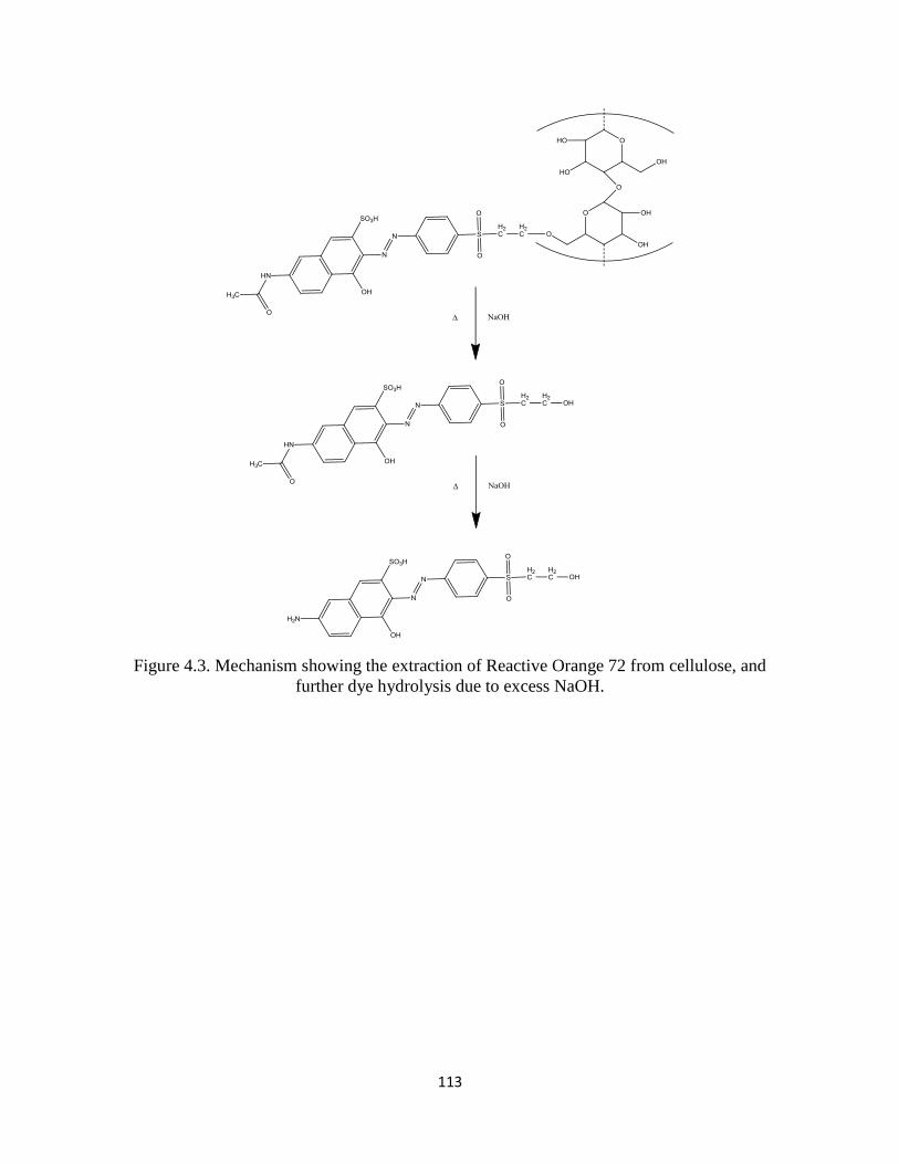
113

Figure 4.3. Mechanism showing the extraction of Reactive Orange 72 from cellulose, and

further dye hydrolysis due to excess NaOH.

114

Figure 4.4. Chromatogram showing the separation of all three reactive dyes. Some dyes

have multiple components. Peak 1 is Reactive Blue 220, peak 2 is Reactive Orange 72,

and peak 3 is Reactive Yellow 160.

0.5 1 1.5 2 2.5 3

0

1

2

3

4

x 106

Retention time (min)

Absorb

ance (

counts

)

1

2

3

115

Figure 4.5. Multiple reactive dye components in the chromatographic region of 0.8 to 2.6

min from Figure 4. Peaks labeled with a 1 are Reactive Blue 220, peaks labeled with a 2

are Reactive Orange 72, and peaks labeled with a 3 are Reactive Yellow 160.

1 1.5 2 2.5-5

0

5

10x 10

5

Retention time (min)

Absorb

ance (

counts

)1

2

3

1

1

2

2

2

3

3

3

3

116

Figure 4.6. (Left) UPLC chromatograms for Reactive Orange 72 standard and (right)

extracted (standard treated with NaOH and heat).

117

Figure 4.7. Areas of both peaks observed after treatment of Reactive Orange 72 with

varying amounts of NaOH. 100% represents 9.375E-7 moles of NaOH to 1 ng of dye.

0

1000

2000

3000

4000

5000

6000

7000

8000

0% 20% 40% 60% 80% 100% 120% 140% 160%

Pe

ak A

rea

NaOH

Peak D'

Peak D''

118

Figure 4.8. Total ion chromatogram of Reactive Yellow 160 standard and isolated

molecular ions of four dye derivatives.

119

Figure 4.9. Total ion chromatogram of the Reactive Yellow 160 standard, isolated

molecular ions of the potential dye derivatives, and their corresponding UV/visible

absorbance spectra.

120

Figure 4.10. TIC of Reactive Yellow 160 after being treated with NaOH and heat

(100°C). Two products were visible by HPLC-MS.

121

Figure 4.11. TIC of Reactive Orange 72 showing the only visible chromatographic peak

and its mass spectra.

122

Figure 4.12. Extracted ion chromatograms for m/z 572, 474, 492, and 417 from the

analysis of Reactive Orange 72. Individual chromatographic peaks for each mass suggest

multiple compounds present in the standard.

123

Figure 4.13. TIC and mass spectra of Reactive Orange 72 after treatment with NaOH and

heat (100°C).

124

Figure 4.14. Calibration model for Reactive Blue 220.

0 500 1000

0

1

2

3

x 104

Concentration (ppb)

Peak a

rea (

counts

)

125

Figure 4.15. Calibration Model for Reactive Orange 72.

0 500 1000

0

1

2

3

4

5

x 104

Concentration (ppb)

Peak a

rea (

counts

)

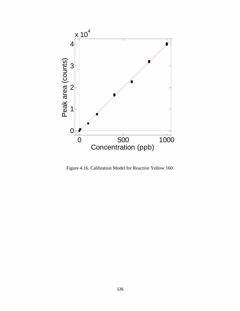
126

Figure 4.16. Calibration Model for Reactive Yellow 160.

0 500 1000

0

1

2

3

4

x 104

Concentration (ppb)

Peak a

rea (

counts

)

127

Figure 4.17. UPLC-DAD chromatograms of extracted Reactive Yellow 160 from a 10

mm fiber (top), a 5 mm fiber (middle) and a 1 mm fiber (bottom).

1.7 1.8 1.9 2

-4.5

-4

-3.5

x 105

Retention time (min)

Absorb

ance (

counts

)

1.7 1.8 1.9 2

-4

-3.5

-3

-2.5

x 105

Retention time (min)

Absorb

ance (

counts

)

1.7 1.8 1.9 2

-3

-2

-1

0

1x 10

5

Retention time (min)

Absorb

ance (

counts

)

128

CHAPTER FIVE

MANDEL SENSITIVITY APPLIED TO ANALYTICAL METHOD PERFORMANCE

COMPARISONS AND LIMITS OF DETECTION

129

ABSTRACT

The concept of the sensitivity ratio as an analytical performance characteristic was

introduced by John Mandel of the National Bureau of Standards in 1954, but has been not

been widely applied in analytical chemistry. The basis for Mandel sensitivity is reviewed

here, along with examples of its use. Because the sensitivity ratio is independent of the

scale in which measurements are expressed, it is a useful tool for comparisons of

variability between different analytical methods.

INTRODUCTION

Validation of a chemical measurement process (CMP) typically involves the reporting

of accuracy, precision, limit of detection, and other figures of merit. Such measures are

often used to decide which approach should be employed in favor of another. Mandel

points out that accuracy comparisons are usually not are contingent on meeting just a few

requirements: (a) a monotonic functional relation must exist between what is measured

and the property to be determined; (b) reference materials having known values must be

available over the target range of the property to be studied; and, (c) the calibration model

must be sufficiently free of both random and systematic errors to establish a clear and

unbiased relationship.1,2

Further, statistical measures of calibration accuracy are available

for assessing the accuracy performance of a calibration function established by

regression.3,4

Comparing CMP performance based on estimates of variability from different

measurement methods and assigning a level of technical merit to a relevant performance

characteristic, however, can be problematic. The oft-recommended approach is to report

relative standard deviations (RSDs) or, equivalently, coefficients of variation (CVs) for

130

the two methods Otto-Hanson, et al. provides an illustrative example for which the

different measurement scales confound comparison.5 With two measurements of daily

temperature at certain different times and locations expressed in Celsius and Fahrenheit

degrees, Assuming that one measurement has a mean of 50 F with a standard deviation

of 10 F, and the other a mean of 10 C with a standard deviation of 5.6 C. With relative

standard deviations of 20% and 56%, it might seem that Fahrenheit measurements are

more reliable. This comparison is invalid because Fahrenheit and Celsius scales are not

proportional to one another because they are interval scale measurements without a

meaningful origin, or zero point.6. In this case, the relationship between the two

measurements is known and the numbers could be converted into the other. In general,

the relationship between measurements having different scales may not be known.

Mandel sensitivity can be applied to comparisons of CMPs on different scales

because it is a scale independent. The computations are trivial, depending only on the

slope of the calibration lines and estimates of the variability of the measurement methods

to be compared.

STATISTICAL BACKGROUND FOR MANDEL SENSITIVITY

Conventional sensitivity

The conventional sensitivity (S) of a CMP is defined as the change in the measured

signal (y) divided by the change in the property being measured (x), i.e., the slope of

the calibration relationship:

S = y / x (1)

131

Figure 5.1 represents the calibration relationship for two different chromatographic

methods of determining the same analyte. The first (upper blue line) method has a

sensitivity of

(2)

The second method (lower red line) has a sensitivity of

(3)

Because of the steeper slope, it appears that the first method is better (more sensitive).

Mandel response

The straight-line calibration relationships represent idealized models of the real

behavior of the chromatographic methods, idealized in the sense that they ignore noise or

uncertainty in the measured data. A more realistic view of variation in the

chromatographic results for these two methods is shown by the numerous individual data

points in Figure 5.2. The calibration lines show what might be expected on the average;

the dots show what might be obtained if many individual measurements were made on

these two systems. Although the first method has the greater sensitivity (y/x = 1.0

count g-1

vs. 0.5 count g-1

), it also has greater noise (b = 5 counts vs. 2 counts).

The noise associated with the first chromatographic method is illustrated in two ways

in the Figure 5.3. The point at (25 g, 25 counts) is shown with a window extending one

standard deviation of the blank (b = 5 counts) above, and one standard deviation below.

The Gaussian curve to the left in the figure is another way of illustrating the uncertainty

of the data point at (25 g, 25 counts). It is a projection of the uncertainty onto the signal

axis (chromatographic peak area). The Gaussian curve is centered at 25 counts, with

marked lines drawn at ±b as "verticals" within the Gaussian. For the first

-1Δy 100 counts= =1.0 counts μg

Δx 100 μg

-150 counts0.5 counts μg

100 μg

y

x

132

chromatographic method, b = 5.0 counts, and the Mandel response for the data point

above 25 g is

(4)

The vertical scale at the right of the plot shows the Mandel response. Note that the

conventional response of 25 counts corresponds to a Mandel response of 5.

Similarly, the noise associated with the second chromatographic method is illustrated

in two ways in Figure 5.4. The point at (50 g, 25 counts) is shown with another window

extending one standard deviation of the blank (b = 5 counts) above, and one standard

deviation below. Again, the Gaussian curve to the left in the figure is a projection of the

uncertainty onto the signal axis. In this case, the Gaussian is centered at 25 counts, with

marked lines drawn at ±b as "verticals" within the Gaussian.

Mandel sensitivity

Mandel defined sensitivity as the ability of a test method to detect a change in the

amount of the property under study.1,2

This ability depends (in part) on the precision of

the CMP. Mandel suggested measuring the response as unitless multiples of the standard

deviation of the blank (b): yM = y / b. The Mandel sensitivity, SM, is defined in the same

way as traditional sensitivity, however, for Mandel response, yM, replaces Δy in the

sensitivity calculation. Thus, the Mandel sensitivity (SM) is defined as the change in the

Mandel response (yM) divided by the change in the property (x):

SM = yM/x = (y/b) / x = (y/x)/b = S/b (5)

For the first method (with the steeper slope), the Mandel sensitivity is

25 counts5.0

5.0 countsM

b

yy

-1-1(1.0 counts μg )

/ 0.20 μg5.0 counts

M bS S

133

The second (less sensitive) method, for which b = 2.0 counts, has a Mandel sensitivity

(SM) of

(6)

The Mandel sensitivity is a slope. It can be interpreted as the number of standard

deviations of the blank that the signal changes per unit change in analyte amount. The

Mandel sensitivity removes the original response measurement units (peak area), and has

units of reciprocal amount (in this case, g-1

).

Although the first method had a larger conventional sensitivity (1.0 counts g-1

vs. 0.5

counts g-1

), the second method has the larger Mandel sensitivity (0.25 g-1

vs. 0.20 g-

1). Because Mandel sensitivity is "the ability of a test method to detect a change in the

amount of the property under study," the second method (with the shallower slope) will

be better able to detect a change in the amount of analyte.

The Mandel response concept lends itself to depicting the performance of two CMPs

on a common scale for comparison. When the two chromatographic methods are plotted

in Figure 5.5 on the same vertical scale of Mandel response, it is clear that the second

method, which had the smaller conventional sensitivity, has the larger Mandel sensitivity

(0.25 g-1

). The first method, which had the larger conventional sensitivity, is seen to

have the smaller Mandel sensitivity (0.20 g-1

). Note that the scaled noise in this plot is

the same for both methods (as it should be on this common scale).

Detection decision limits

Mandel's original sensitivity paper was motivated by the concept of deciding whether

two CMP responses close to one another can be discriminated—a decision process that is

related to calculating decision levels associated with analyte detection. The common

-1-1(0.5 counts μg )

/ 0.25 μg2.0 counts

M bS S

134

Mandel response scale is an elegant path to calculate such decision limits, because these

limits are all based on multiples of the standard deviation of the blank (b), the very

quantity that is measured by the Mandel response. Before discussing the application of

Mandel sensitivity to CMP detection limits, we review the basis for the common critical

decisions limits for analyte detection.

The limit of detection (LD) is specified by calculating the signal level above the mean

of the blank at which the fraction risk of concluding that analyte is present, when it

actually is not present, is acceptably small. Assuming a Gaussian distribution of noise for

measurements of a sample containing no analyte (the 'blank'), an estimate of the standard

deviation is obtained by replicate measurements of a blank, or by other statistical

approaches, and assumed to have sufficient reliability to be considered a good estimate of

the population standard deviation of the CMP. Because the variability of many CMPs is

homoscedastic at low levels of analyte, the standard deviation of the blank, b, is usually

a good estimate of the uncertainty around the LD. This decision limit is calculated by

finding the number (k) of standard deviations above the mean that provides an acceptably

low upper-tailed area above that level. A common choice for this criterion is k = 3, which

provides an upper-tailed area of = 0.0014. This probability can be interpreted as the

false positive risk of obtaining a response as high as or higher than LD from a sample that

contains no analyte. Equivalently, the level of confidence associated with correct

detection decision at this level is 100% (1 - ), or 99.86 %. No single value of k is

appropriate for all situations. For example, k = 3.3 provides higher detection reliability

with a level of confidence for correct detection of 99.95 %, and a fractional false positive

probability of = 0.0005. The amount of analyte equivalent to the limit of detection (on

135

the signal axis) is the limit of detection amount (LDA) and is found by inverting the

calibration relationship. If a straight line calibration (y = mx + b, where y is detector

response, x is analyte amount, m is the slope, and b is the y-intercept) is assumed and

using k = 3.3,

(7)

However, at k = 3 or k = 3.3 for the LDA, the false negative error rate ( ) is

unacceptably high: 50% of time samples containing analyte present at that LDA will be

falsely declared not detected. Remarkably, the risk has historically been often ignored,

even in standards documents from regulatory authorities.7,8

The recognition of false negative () risk leads to another critical limit, the minimum

consistently detectable amount (MCDA). The MCDA represents the amount at which

analyte can be said to be consistently detected, i.e., where the false negative error rate is

reduced to be equivalent to the false positive error rate. With the signal domain

measurement 6 standard deviations of the blank above the mean of the blank, the

fractional risk of encountering a sample giving a signal below the LD is 0.0014. At 6.6

standard deviations of the blank above the mean of the blank, the fractional risk of a false

negative result occurring below the LDA is 0.0005. Thus, the MCDA might be calculated

as

(8)

Analyte amounts above the LDA support the detection decision with high confidence, but

do so without controlling the false negative risk. Analyte detected at or above the MCDA

are associated with a detection confidence of at least 99.95 % and a false negative risk

6.6 bsMCDA

m

3.3 bsLDA

m

136

of 0.0005. The low false negative error rate at the MCDA insures that analyte at or above

this limit is consistently detected.

At an analyte concentration equal to the LDA, the expected % relative standard

deviation (%RSD) of measurements can be calculated from the standard deviation of the

blank b projected to the amount axis as the standard deviation of predicted analyte

amount, a:

(9)

The %RSD at an analyte concentration equal to the MCDA is:

(10)

These %RSD values are too uncertain for the resulting measurements to be considered

quantitative (no analytical chemist would boast of achieving a 30.30 %RSD). The

generally accepted signal-to-noise ratio considered to be quantitative is 10:1, or

equivalently and %RSD of 10 %. Thus, the limit of quantitation (LQ) is defined as the

concentration of analyte that produces a signal 10 times the standard deviation of noise

(defined by the standard deviation of the blank),

(11)

At analyte levels between the MCDA and the LQ, analyte is consistently detected with

high confidence and low false negative errors, but the %RSD is insufficiently to

guarantee accurate quantitation unbiased by experimental uncertainty.

Applying Mandel sensitivity to detection decision limits

Calibrations from the two chromatographic methods discussed earlier are plotted on

again on the same vertical scale of Mandel response in Figure 5.6. The LDA (with k =

3.3) for both methods can be calculated from the Mandel sensitivity as

% 100% 30.30%3.3

a

a

RSD

% 100% 15.15%6.6

a

a

RSD

% 100% 10%10

a

a

RSD

137

(12)

For the first chromatographic method, with SM = 0.20 µg-1

,

For the second chromatographic method, with SM = 0.25 µg-1

,

These LDA values are the analyte amounts (on the x-axis in Figure 5.6 ) at which the

horizontal green line at height 3.3b intersects with the respective calibration lines.

The MCDA (with k = 6.6) for both methods can be calculated from the Mandel

sensitivity as

(12)

For the first chromatographic method, with SM = 0.20 µg-1

,

(13)

For the second chromatographic method, with SM = 0.25 µg-1

,

(14)

These MCDA values occur in Figure 5.7 at the intersection of the horizontal green line at

6.6b with the Mandel response calibration lines.

Finally, the LQ (with k = 10) for both methods can be calculated from the Mandel

sensitivity as

(15)

For the first chromatographic method, with SM = 0.20 µg-1

,

For the second chromatographic method, with SM = 0.25 µg-1

,

3.3

m

LDAS

1

3.316.5

0.20LDA g

g

1

3.313.2

0.25LDA g

g

1

6.633.0

0.20MCDA g

g

1

6.626.4

0.25MCDA g

g

6.6

M

MCDAS

1

1050.0

0.20LQ g

g

1

6.640.0

0.25LQ g

g

10

M

LQS

138

These MCDA values occur in Figure 5.8 at the intersection of the horizontal green line at

10b with the Mandel response calibration lines.

Conclusions

Evaluating a CMP form the viewpoint of Mandel response and Mandel sensitivity

offers an easy and rapid method for comparison of the calibration performance of

analytical methods by use of scale independent approach. The Mandel sensitivity offers

an advantage over scale dependent approaches such as RSDs and CVs because it

normalizes performance relative to the variability of the measurement method. Mandel

sensitivity allows for calculation of detection limit critical values in a universal way that

also provides intuitive and visual understanding of the differences among limit of

detection amount, minimal consistently detectable amount, and limit of quantitation. We

recommend its use for comparing the calibration performance of different analytical

methods.

Coauthors of this work include Stanley N. Deming (Statistical Designs, Houston, TX)

and Stephen L. Morgan (Department of Chemistry and Biochemistry, University of South

Carolina, Columbia, SC 29208). Research in this presentation was supported by award

2010-DN-BX-K245 from the National Institute of Justice, Office of Justice Programs, U.

S. Department of Justice. The opinions, findings, and conclusions or recommendations

expressed in this publication are those of the author(s) and do not necessarily reflect those

of the Department of Justice. Mention of commercial products does not imply

endorsement on the part of the National Institute of Justice or the University of South

Carolina.

139

REFERENCES

(1) Mandel, J.; Stiehler, R. D. Sensitivity—A criterion for the comparison of methods

of test, Journal of Research of the National Bureau of Standards 1954, 53, 155-

159.

(2) Mandel, J. The Statistical Analysis of Experimental Data, John Wiley & Sons, Inc.,

New York, 1964, pp. 363-389.

(3) Draper, N. R; Smith, S. Applied Regression Analysis, 3rd

ed., John Wiley & Sons,

Inc., New York, 1998.

(4) Deming, S. N.; Morgan, S. L. The use of linear models and matrix least squares in

clinical chemistry, Clin. Chem. 1979, 25, 840-855.

(5) Otto-Hanson, L.; Eskridge, K. M.; Steadman; J. R.; Madisa, G. The sensitivity

ratio: A superior method to compare plant and pathogen screening tests. Crop Sci.

2009, 49(1), 153-160.

(6) Stevens, S. S. On the theory of scales of measurement. Science 1946, 677-680.

(7) Currie, L. A. Detection: Overview of historical, societal, and technical issues.

Chapter 1 in: Detection in Analytical Chemistry: Importance, Theory, and

Practice, L. A. Currie (ed.), American Chemical Society, Washington, DC, 1988.

(8) Currie, L. A. Detection: International update, and some emerging di-lemmas

involving calibration, the blank, and multiple detection decisions. Chemom, Intell.

Lab. Sys. 1997, 37, 151-181.

140

Figure 5.1. Calibration relationship for two different measurement processes.

Figure 5.2. Calibration relationship for two different measurement processes with noise;

standard deviation for upper (blue) calibration is 5 counts, and the standard deviation for

the lower (red) calibration is 2 counts.

141

Figure 5.3. Calibration relationship for the first method with plus and minus one standard

deviation window about the response of 25 peak counts for 25 micrograms. The right

hand scale shows the Mandel response in unitless multiples of the standard deviation.

Figure 5.4. Calibration relationship for the second method with plus and minus one

standard deviation window about the response at 25 peak counts for 50 micrograms. The

right hand scale shows the Mandel response in unitless multiples of the standard

deviation.

142

Figure 5.5. Common Mandel response scale for comparison of calibration performance.

The second (red) method has larger Mandel sensitivity (0.25 µg-1

) than the

first (blue) method (0.20 µg-1

).

Figure 5.6. Common Mandel response scale for estimation of LDA. The second (red)

method has a lower LDA (13.2 µg) than the first (blue) method (16.5 µg).

143

Figure 5.7. Common Mandel response scale for estimation of MCDA. The second (red)

method has a lower MCDA (26.4 µg) than the first (blue) method (33.0 µg).

Figure 5.8. Common Mandel response scale for estimation of LQ. The second (red)

method has a lower LQ (40.0 µg) than the first (blue) method (50.0 µg).

144

WORKS CITED

Andreasen, M. F.; Telving, R.; Birkler, R.I.D.; Schumacher, B.; Johannsen, M. A fatal

poisoning involving Bromo-Dragonfly. Forensic Sci. Int. 2009, 183, 91–96.

Beattie, B.; Roberts, H.; Dudley, R. J. The extraction and classification of dyes from

cellulose acetate fibers. J. Forensic Sci. Soc. 1981, 21, 233-237.

Beattie, I.B.; Dudley, R.J.; Smalldon, K.W. The extraction and classification of dyes on

single nylon, polyacrylonitrile and polyester fibers. J. Soc. Dye. Colour 1979, 95, 295-

302.

Bendroth, P.; Kronstrand, R.; Helander, A.; Greby, J.; Stephanson, N.; Krantz, P.

Comparison of ethyl glucuronide in hair with phosphatidylethanol in whole blood as

post-mortem markers of alcohol abuse. Forensic Sci. Int. 2008, 176, 76-81.

Borros, S.; Barbera, G.; Biada, J.; Agullo, N. The use of capillary electrophoresis to study

the formation of carcinogenic aryl amines in azo dyes. Dyes and Pigm. 1999, 43, 189-

196.

Bozic, M.; Kokol, V. Ecological alternatives to the reduction and oxidation processes in

dyeing with vat and sulphur dyes. Dyes and Pigments, 2008, 76, 299-309.

Burkinshaw, S.M.; Graham, C. Capillary zone electrophoresis analysis of chlorotriazinyl

reactive dyes in dyebath effluent. Dyes and Pigm. 1997, 34, 307-319.

Burkinshaw, S.M.; Hinks, D.; Lewis, D.M. Capillary zone electrophoresis in the analysis

of dyes and other compounds employed in the dye-manufacturing and dye-using

industries. J. Chromatogr. A 1993, 640, 413-417.

Burkinshaw, S.M.; Hinks, D.; Lewis, D.M. The use of capillary electrophoresis for the

analysis of several dye classes. In: Special Publication - Royal Society of Chemistry

1993,122, 93-100.

Christie, R. Colour Chemistry. RSC Paperbacks: Cambridge, England, 2001.

Crabtree, S. R.; Rendle, D. F.; Wiggins, K. G.; Salter, M. T. The Release of Reactive

Dyes from Wool Fibers by Alkaline- Hydrolysis and Their Analysis by Thin-Layer

Chromatography. J. Soc. Dye. Colour 1995, 111, 100-102.

145

Croft, S.N.; Hinks, D. Analysis of dyes by capillary electrophoresis. Textile Chemist and

Colorist 1993, 25, 47-51.

Croft, S.N.; Hinks, D. Analysis of dyes by capillary electrophoresis. J. Soc. Dye. Colour

1992, 108, 546-551.

Croft, S.N.; Lewis, D.M. Analysis of reactive dyes and related derivatives using high-

performance capillary electrophoresis. Dyes and Pigm. 1992, 18, 309-317.

Currie, L. A. Detection: International update, and some emerging di-lemmas involving

calibration, the blank, and multiple detection decisions. Chemom, Intell. Lab. Sys. 1997,

37, 151-181.

Currie, L. A. Detection: Overview of historical, societal, and technical issues. Detection

in Analytical Chemistry: Importance, Theory, and Practice, L. A. Currie (ed.), American

Chemical Society, Washington, DC, 1988.

Deadman, H. Fiber evidence and the Wayne Williams trial, US Government Document

J1.14/8a:F44, Federal Bureau of Investigation, US Department of Justice, FBI Law

Enforcement Bulletin, March and May, 1984.

Deming, S. N.; Morgan, S. L. Experimental Design: A Chemometric Approach, 2nd ed.

Elsevier Science Publishers: Amsterdam, 1993.

Deming, S. N.; Morgan, S. L. The use of linear models and matrix least squares in

clinical chemistry, Clin. Chem. 1979, 25, 840-855.

Dockery C. R., Stefan, A. R., Nieuwland, A. A., Roberson, S. N., Baguley, B.M.,

Hendrix, J. E., Morgan, S. L. Automated extraction of direct, reactive, and vat dyes from

cellulosic fibers for forensic analysis by capillary electrophoresis. Anal. Bioanal. Chem.

2009, 394, 2095-2103.

Draper, N. R; Smith, S. Applied Regression Analysis, 3rd

ed., John Wiley & Sons, Inc.,

New York, 1998.

Eyring, M. B.; Gaudette, B. D. An introduction to the forensic aspects of textile fiber

examinations. Chapter 6 in: Forensic Science Handbook, vol. 2, R. Saferstein, Ed.;

Prentice Hall: Englewood Cliffs, NJ, 2005.

Fisher, J. Forensics under Fire: Are Bad Science and Dueling Experts Corrupting

Criminal Justice? Rutgers University Press: New Brunswick, NJ, 2008.

Gaudette, B. D. The forensic aspects of textile fiber examination. Chapter 5 in: Forensic

Science Handbook, vol. 2, R. Saferstein, Ed.; Prentice Hall: Englewood Cliffs, NJ, 1988.

Grieve, M. Interpretation of fibres evidence. Chapter 13 in: Forensic Examination of

Fibres, 2nd edition, Robertson J.; Grieve, M., Eds.; Taylor & Francis: London, 1999.

146

Hartshorne, A. W.; Laing, D. K. The dye classification and discrimination of colored

polypropylene fibers. Forensic Sci.Int. 1984, 25, 133-141.

Hartzell-Baguley, B.; Stefan, A. R.; Dockery, C. R.; Hendrix, J. E.; Morgan, S. L. Non-

aqueous capillary electrophoresis of azo and anthraquinone disperse dyes extracted from

polyester fibers for forensic analysis. Anal. Bioanal. Chem., 2009, unpublished

manuscript.

Home, J. M.; Dudley, R. J. Thin-layer chromatography of dyes extracted from cellulosic

fibers. Forensic Sci.Int. 1981, 17, 71-78.

Home, J.; Dudley, R. Thin-layer chromatography of dyes extracted from cellulosic fibres.

Forensic Sci.Int. 1981, 17, 71–78.

Houck, M. Statistics and trace evidence: the tyranny of numbers, Forensic Science

Communications, 1 January 1999.

Huang, M.; Russo, R.; Fookes, B. G.; Sigman, M. E. Analysis of Fiber Dyes by Liquid

Chromatography Mass Spectrometry (LC-MS) with Electrospray Ionization:

Discriminating Between Dyes with Indistinguishable UV-Visible Absorption Spectra. J.

Forensic Sci. 2005, 50, 526-534.

Huang, M.; Yinon, J.; Sigman, M. E. Forensic identification of dyes extracted from

textile fibers by liquid chromatography mass spectrometry (LC-MS). J. Forensic Sci.

2004, 49, 238-249.

Ji, C.; Feng, F.; Chen, Z.; Chu, X. Highly sensitive determination of 10 dyes in food with

complex matrices using SPE followed by UPLC-DAD-Tandem mass spectrometry. J.

Liq. Chromatogr. & Relat. Technol. 2011, 34, 93-105.

Kelly, J. F.; Wearner, P. K. Tainting Evidence: Inside the Scandals at the FBI Crime Lab,

The Free Press: New York, 1998.

Laing, D. K.; Boughey, L.; Hartshorne, A. W. The standardization of thin layer

chromatographic systems for comparison of fiber dyes. J. Forensic Sci. Soc. 1990, 30,

299-307.

Laing, D. K.; Gill, R.; Blacklaws, C.; Bickley, H.M. Characterization of acid dyes in

forensic fiber analysis by high-performance liquid chromatography using narrow-bore

columns and diode array detection. J. Chromatogr. 1988, 442, 187-208.

Laing, D. K.; Hartshorne, A. W.; Bennett, D. C. Thin layer chromatography of azoic dyes

extracted from cotton fibers. J. Forensic Sci. Soc. 1990, 30, 309-315.

Macrae, R.; Dudley, R. J.; Smalldon, K. W. The characterization of dyestuffs on wool

fibers with special reference to microspectrophotometry. J. Forensic Sci. 1979, 24, 117-

129.

147

Macrae, R.; Smalldon, K.W. The characterization of dyestuffs on wool fibers with special

reference to microspectrophotometry. J .Forensic Sci. 1979, 24, 109-116.

Mandel, J. The Statistical Analysis of Experimental Data, John Wiley & Sons, Inc., New

York, 1964, pp. 363-389.

Mandel, J.; Stiehler, R. D. Sensitivity—A criterion for the comparison of methods of test,

Journal of Research of the National Bureau of Standards 1954, 53, 155-159.

Minioti, K.; Sakellariou, C.; Thomaidis, N. Determination of 13 synthetic food colorants

in water-soluble foods by reversed-phase high-performance liquid chromatography

coupled with diode-array detector. Anal. Chim. Acta, 2007, 583, 103-110.

Morgan, S. L.; Vann, B. C.; Baguley, B. M.; Stefan, A. R. Advances in discrimination of

dyed textile fibers using capillary electrophoresis/mass spectrometry. Trace Evidence

Symposium, Clearwater, FL, 2007

National Research Council of the National Academies. Forensic Analysis: Weighing

Bullet Lead Evidence. The National Academies Press: Washington, DC, 2004.

National Research Council of the National Academies. Strengthening Forensic Science in

the United States: A Path Forward, The National Academies Press: Washington, DC,

2009.

Needles, H. L. Textile Fibers, Dyes, Finishes, and Processes: A Concise Guide. Noyes

Publications: Park Ridge, NJ, 1986.

Oien, C. T. Case management issues from crime scene to courtroom. Trace Evidence

Symposium, Clearwater, FL, 2007 [URL: http://nfstc.org/projects/trace/].

Otto-Hanson, L.; Eskridge, K. M.; Steadman; J. R.; Madisa, G. The sensitivity ratio: A

superior method to compare plant and pathogen screening tests. Crop Sci. 2009, 49, 153-

160.

Pawlak, K.; Puchalska, M.; Miszczak, A.; Rosloniec, E.; Jarosz, M. Blue natural organic

dyestuffs – from textile dyeing to mural painting. Separation and characterization of

coloring matters present in elderberry, longwood and indigo. J. Mass Spectrom. 2006, 41,

613-622.

Petrick, L.M.; Wilson, T.A.; Fawcett, W.R. High-performance Liquid Chromatography-

Ultraviolet-Visible Spectroscopy-Electrospray Ionization Mass Spectrometry Method for

Acrylic and Polyester Forensic Fiber Dye Analysis. J. Forensic Sci. 2006, 51, 771-779

Petroviciu, I.; Albu, F.; Medvedovici, A. LC/MS and LC/MS/MS based protocol for

identification of dyes in historic textiles.‖ Microchemical Journal, 2010, 95, 247-254.

148

Rafaëlly, L.; Héron, S.; Nowik, W.; Tchapla, A. Optimization of ESI-MS detection for

the HPLC of anthraquinone dyes. Dyes and Pigm. 2008, 77, 191-203.

Rendle, D. F.; Crabtree, S. R.; Wiggins, K. G.; Salter, M. T. Cellulase Digestion of

Cotton Dyed with Reactive Dyes and Analysis of the Products by Thin-Layer

Chromatography. J. Soc. Dye. Colour 1994, 110, 338-341.

Rendle, D. F.; Wiggins, K. G. Forensic analysis of textile fibre dyes. Review of Progress

in Coloration and Related Topics 1995, 25, 29-34.

Resua, R. A semi-micro technique for the extraction and comparison of dyes in textile

fibers. J. Forensic Sci. 1980, 25, 168-173.

Riu, J.; Barcelo, D. Determination of linear alkylbenzene sulfonates and their polar

carboxylic degradation products in sewage treatment plants by automated solid-phase

extraction followed by capillary electrophoresis-mass spectrometry. Analyst 2001, 126,

825-828.

Riu, J.; Eichhorn, P.; Guerrero, J.A.; Knepper, T.P.; Barcelo, D. Determination of linear

alkylbenzenesulfonates in wastewater treatment plants and coastal waters by automated

solid-phase extraction followed by capillary electrophoresis-UV detection and

confirmation by capillary electrophoresis-mass spectrometry. J. Chromatogr. A 2000,

889, 221-229.

Riu, J.; Schonsee, I.; Barcelo, D. Determination of sulfonated azo dyes in groundwater

and industrial effluents by automated solid-phase extraction followed by capillary

electrophoresis mass spectrometry. J. Mass Spectrom. 1998, 33, 653-663.

Robertson J.; Grieve, M., Eds., Forensic Examination of Fibres. 2nd edition. London:

Taylor & Francis: 1999.

Robertson, J.; Wells, R.J.; Pailthorpe, M.T.; David, S.; Aumatell, A.; Clark, R. An

assessment of the use of capillary electrophoresis for the analysis of acid dyes in wool

fibers. Advances in Forensic Sciences, Proceedings of the Meeting of the International

Association of Forensic Sciences, 13th, Duesseldorf, Aug. 22-28, 1995, 4, 247-249.

Roux, C.; Margot, P. The population of textile fibres on car seats. Sci Justice 1997, 37,

25-30.

Shaw, I. C. Micro-scale thin-layer chromatographic method for the comparison of dyes

stripped from wool fibers. Analyst 1980, 105, 729-730.

Shore, J. Colorants and Auxiliaries, vol. 1, 2nd edition. Society of Dyers and Colourists,

West Yorkshire: England, 2002; pp. 18–23.

149

Sirén, H.; Sulkava, R. Determination of black dyes from cotton and wool fibers by

capillary zone electrophoresis with UV detection: application of marker technique. J.

Chromatogr. A 1995, 717, 149-155.

Smith, W. F. Experimental Design for Formulation. Cambridge University Press: New

York, 2005.

Stefan, A. R., Dockery C. R., Nieuwland, A. A., Roberson, S. N., Baguley, B. M.,

Hendrix, J. E., Morgan, S. L. Forensic analysis of anthraquinone, azo, and metal complex

acid dyes from nylon fibers by micro-extraction and capillary electrophoresis. Anal.

Bioanal. Chem. 2009, 394, 2077-2085.

Stefan, A. R., Dockery, C. R., Baguley, B.M., Vann, B. C., Nieuwland, A. A., Hendrix, J.

E., Morgan, S. L. Microextraction, capillary electrophoresis, and mass spectrometry for

forensic analysis of azo and methine basic dyes from acrylic fibers. Anal. Bioanal.

Chem.2009, 394, 2087-2094.

Stevens, S. S. On the theory of scales of measurement. Science 1946, 677-680.

Stoney. D.A. The assumption of relevance and an application to one-trace and two-

Relaxation of trace problem. J. Forensic Sci. Soc. 1994, 34, 17-21.

Szostek, B.; Orska-Gawrys, J.; Surowiec, I.; Trojanowicz, M. Investigation of natural

dyes occurring in historical Coptic textiles by high-performance liquid chromatography

with UV-Vis and mass spectrometric detection. J. Chromatogr. A 2003, 1012, 179-192.

Takeda, S.; Tanaka, Y.; Nishimura, Y.; Yamane, M.; Siroma, Z.; Wakida, S. Analysis of

dyestuff degradation products by capillary electrophoresis. J. Chromatogr. A 1999, 853,

503-509.

The Warren Commision Report. St. Martin's Press, New York, 1964; p. 592.

Tuinman, A.A.; Lewis, L.A.; Lewis, S.A. Trace-fiber color discrimination by

electrospray ionization mass spectrometry: A tool for the analysis of dyes extracted from

submillimeter nylon fibers. Anal. Chem. 2003, 75, 2753-2760.

Watt, R.; Roux, C.; Robertson, ―The population of coloured textile fibres in domestic

washing machines. J. Sci Justice 2005, 45,75-83.

Webb-Salter, M.; Wiggins, K. G. Aids to Interpretation, in: Forensic Examination of

Fibres. 2nd edition, J. Robertson, M. Grieve, Eds., Taylor & Francis: London, 1999; pp.

364-378.

Wheals, B.B.; White, P.C.; Paterson, M.D. High-performance liquid chromatographic

method utilizing single or multi-wavelength detection for the comparison of disperse

dyes extracted from polyester fibers. J. Chromatogr. 1985, 350, 205-215.

150

Wiggins, K. G. Thin layer chromatographic analysis for fibre dyes. Chapter 11 in:

Forensic Examination of Fibres, 2nd edition, Robertson J.; Grieve, M., Eds.; Taylor &

Francis: London, 1999.

Wiggins, K. G.; Crabtree, S. R.; March, B. M. The importance of thin layer

chromatography in the analysis of reactive dyes released from wool fibers. J. Forensic

Sci. 1996, 41, 1042-1045.

Wiggins, K.; Holness, J. A further study of dye batch variation in textile and carpet

fibres. Science & Justice 2005, 45, 93-96.

Wiggins, K.G.; Cook, R.; Turner, Y.J. Dye batch variation in textile fibers. J. Forensic

Sci. 1988, 33, 998-1007.

Wood, M.; Laloup, M.; Samync, N.; del Mar Ramirez Fernandez, M.; de Bruijn, E. A.;

Maes, R A.A.; De Boeck, G. Recent applications of liquid chromatography-mass

spectrometry in forensic science. J. Chromatogr. A 2006, 1130, 3–15.

Xu, X.; Leijenhorst, H.; Van den Hoven, P.; De Koeijer, J.A.; Logtenberg, H. Analysis of

single textile fibres by sample-induced isotachophoresis-micellar electrokinetic capillary

chromatography. Sci. Justice 2001, 41, 93-105.

Yinon, J.; Saar, J. Analysis of dyes extracted from textile fibers by thermospray high-

performance liquid chromatography-mass spectrometry. J. Chromatogr. A 1991, 586, 73-

84.

Zhang, X.; Laursen, R. Development of Mild Extraction Methods for the Analysis of

Natural Dyes in Textiles of Historical Intersest Using LC-Diode Array Detector-MS.

Anal. Chem. 2005, 77, 2022-2025.