DEVELOPMENT AND EVALUATION OF INCIDENT-DETECTION ALGORITHMS FOR ELECTRONIC-DETECTOR SYSTEMS ON FREEWAYS

Masami Sakasita, De Leuw, Cather and Company; and Adolf D. May, Institute of Transportation and Traffic Engineering,

University of California, Berkeley

This paper describes a study of the development and evaluation of incident­detection algorithms for electronic-detector systems on freeways. The study was in 3 parts. The first part reviewed existing detection algorithms and the development of 2 new detection algorithms. During the develop­ment of these 2 algorithms, a section of a freeway lane formed by 2 detec­tors at both ends was treated as a system, and an attempt was made to express traffic movements by using dynamic equations. The second part involved the development of a microscopic simulation model of freeway traffic performance. The simulation model was capable of simulating traffic conditions on a freeway under incident and nonincident situations. The output of the simulation model, which was recorded at presence detec­tors in each lane at 0.125-mile (0.20-km) spacings, was stored on a mag­netic tape and played back later to test each detection algorithm. The third part evaluated the newly developed algorithms. The California model, which is considered to be the most widely known algorithm, was compared to the 2 proposed algorithms.

•INCIDENT-FREE flow conditions on urban freeways are abnormal. Previous studies have noted that freeway incident rates may be as high as 1 incident per directional mile (0.62 incident per directional kilometer) per hour (1) . Freeway incidents are hazardous to all in the traffic stream. And reduction in freeway capacity may be significant enough to cause congestion and thus create further hazards and delay for passing motorists.

Knowledge of incidents that reduce capacity is extremely important for freeway­control strategies. Previous work has been undertaken by us and by others to evaluate incident-detection systems (!, ~ !). But the development and evaluation of electronic­detector systems have received only limited attention. These systems generally are based on uncontrolled empirical experiments only. The results of these empirical experiments are discussed in the paper.

This paper describes a study of the development and evaluation of incident-detection algorithms for electronic-detector systems. The study consisted of the development of 2 detection algorithms and a simulation model of freeway traffic performance. In addition, the algorithms were evaluated by using the simulation model, TRAFFIC. Two detection algorithms were proposed. One was the dynamic model, which applies the information-theory technique (5). The other was the stream discontinuity model, which is based on a macroscopic treatment of the dynamic model. This study also evaluated the detection algorithms. The California model, which is considered to be the most widely known, was evaluated along with the 2 newly developed algorithms.

AUTOMATIC DETECTION ALGORITHMS

Several unique studies of automatic detection systems have been completed. This paper will describe 2 operational systems and 2 experimental systems.

48

49

Port of New York Authority Method

The Port of New York Authority method is described in detail elsewhere (J_, Q_). Con­trol strategy for the Lincoln Tunnel is based on the number of vehicles in each of 3 sections. If Yk =the number of vehicles in a section at the beginning of the kth obser­vation period, ulk = the number of vehicles that have entered the section in the kth time period, and U2lc =the number of vehicles that have left the section in the kth time period, then the number of vehicles at the beginning of the k + 1 period should be

(1)

The traffic density in each section of the tunnel was estimated by this relation, and in­cidents were predicted for abnormally large values of density. This method, however, accumulates errors because of miscounts by the sensors. Therefore, it requires microscopic identification of vehicles after a certain time. This method can be used in the tunnel because of the tunnel's accurate detection system and because vehicles are not permitted to change lanes in the tunnel. Recently this method was improved by applying the extended Kalman filtering theory to it.

The California Model

The California model (6), which has produced promising results, uses occupancy as a measure of traffic concTitions . It is less accurate than that used in the Lincoln Tunnel in New York. The basic concept of the method is a comparison of occupancies at the neighboring detectors in the same time interval and a comparison of occupancies at adjacent time intervals at the same detector. Occupancies are 1-min values updated every 20 or 30 sec. The detection criterion should predict an incident when all the calculated values of X1, X2, and X3 exceed K1, K2, and & at the same time.

where

OCC1

t X1, X2, X3 Ki, K2, K3

B

occupancy at station i that is counted in the direction of travel, time instant, X occupancy values,

(2)

(3)

(4)

K occupancy values (K1, K2, and &, which can be adjusted depending on location, are 8, 0.55, and 0.10 respectively for the nonpeak period and 8, 0.55, and 0.15 respectively for the peak period), and a time period of 20 or 30 sec (backward shift operator).

Texas Transportation Institute Method

Experimental studies conducted by the Texas Transportation Institute (!!) suggest several

50

new approaches to automatic detection systems, one of which is the kinetic energy ap­proach. Kinetic energy is computed as follows.

Ea: kµ2

that is,

where

E kinetic energy, k density, µ. speed, q flow, and e occupancy.

In a study based on this approach, the 1-min kinetic energy values were compared with preestablished limits and a probable incident was reported whenever the measurements exceeded their lower limits. This approach was extended to an individual-lane-energy approach that was done lane by lane. The results of the experimental study tended to show that this method has a high false-alarm rate.

Double Exponential Smoothing Method

Cook and Cleveland (10) introduced another new approach for automatic incident­detection: a time-series analysis technique called the double exponential smoothing method. In this method, the smoothing function of observation at the t th time incre­ment, St (x), is expressed as

where

a smoothing constant, Xt = t th observation, and

f3 = 1 - ll!.

(5)

Traffic parameters were forecast, and incidents were predicted for parameter values that exceeded the preset limit based on Eq. 5. Experiments have shown that this method is comparable or superior to the California model.

DEVELOPMENT OF INCIDENT-DETECTION ALGORITHMS

To develop incident-detection algorithms, one should treat a section of freeway lane formed by 2 detectors at both ends as a system. An upstream detector would provide the system with certain output traffic measures. This system is shown in Figure 1. In­side the system, vehicles do or do not change lanes. The function of the system is ex­pressed by a travel-time distribution.

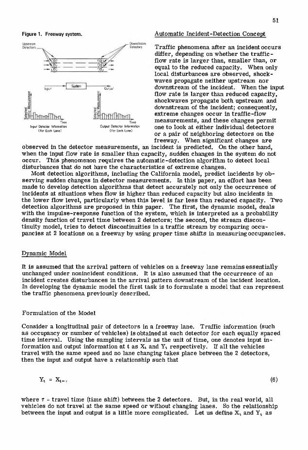
Figure 1. Freeway system.

Upstream Detectors

Input

Time Input Oeteclor Information

(F"or Each Lone)

51

Automatic Incident-Detection Concept

Downslreom oe1ee10<s Traffic phenomena after an incident occurs

Output

,~Lm_ .!!l; .x ....

Time Output Oe1ec1or lnformolion

(For Eoch l one )

differ, depending on whether the traffic­flow rate is larger than, smaller than, or equal to the reduced capacity. When only local disturbances are observed, shock-waves propagate neither upstream nor downstream of the incident. When the input flow rate is larger than reduced capacity, shockwaves propagate both upstream and downstream of the incident; consequently, extreme changes occur in traffic-flow measurements, and these changes permit one to look at either individual detectors or a pair of neighboring detectors on the freeway. When significant changes are

observed in the detector measurements, an incident is predicted. On the other hand, when the input flow rate is smaller than capacity, sudden changes in the system do not occur. This phenomenon requires the automatic-detection algorithm to detect local disturbances that do not have the characteristics of extreme changes.

Most detection algorithms, including the California model, predict incidents by ob­serving sudden changes in detector measurements. In this paper, an effort has been made to develop detection algorithms that detect accurately not only the occurrence of incidents at situations when flow is higher than reduced capacity but also incidents in the lower flow level, particularly when this level is far less than reduced capacity. Two detection algorithms are proposed in this paper. The first, the dynamic model, deals with the impulse-response function of the system, which is interpreted as a probability density function of travel time between 2 detectors; the second, the stream discon­tinuity model, tries to detect discontinuities in a traffic stream by comparing occu­pancies at 2 locations on a freeway by using proper time shifts in measuring occupancies.

Dynamic Model

It is assumed that the arrival pattern of vehicles on a freeway lane remains essentialiy unchanged under nonincident conditions. It is also assumed that the occurrence of an incident creates disturbances in the arrival pattern downstream of the incident location. In developing the dynamic model the first task is to formulate a model that can represent the traffic phenomena previously described.

Formulation of the Model

Consider a longitudinal pair of detectors in a freeway lane. Traffic information (such as occupancy or number of vehicles) is obtained at each detector for each equally spaced time interval. Using the sampling intervals as the unit of time, one denotes input in­formation and output information at t as Xt and Yt respectively. If all the vehicles travel with the same speed and no lane changing takes place between the 2 detectors , then the input and output have a relationship such that

(6)

where 7' = travel time (time shift) between the 2 detectors. But, in the real world, all vehicles do not travel at the same speed or without changing lanes. So the relationship between the input and output is a little more complicated. Let us define Xt and Yt as

52

the respective deviations of t from the mean of input and output information over a long time period. Then output of the RyRtem Yt iR rP.prP.sented as a linear aggregate of input deviations at t, t - 1, t - 2, ... , and the noise sequence, Nt, is such that

Yt = VaXt + V1Xt - 1 + v2Xt - 2 + .•• + Nt

(va + v1B + v2B2 + ••• )Xt + Nt

v(B)Xt + Nt (7)

In the field of time-series analysis, the weights of Vo, v1, ... in Eq. 7 are the impulse­response function of the system and v(B) is the transfer function of the filter. B is defined by BXt = Xt _ 1. The sum of the weights v0 , v1, ... is equal to the steady-state gain of the system, g.

(8)

The steady-state gain inthis application is interpreted as the ratio of the mean values of traffic information at the upstream and downstream detectors. Under nonincident conditions g is assumed to come very close to 1, and v1 represents the travel-time probability between the 2 i detectors.

Nt in Eq. 7 corrupts the linear dynamic system; this is mainly due to lane changing and detector errors. It is assumed that Xt is uncorrelated with Nt.

If it is known that the v1s are effectively zero beyond i = K, then, in order to deter­mine the v1s of the system (N + 1) :<?: (K + 1), sets of Xt and Yt have to be made. Obser­vations would yield equations of the form

(9)

If only K + 1 sets of measurements are made, then unique solutions would exist for Vu

but noise and measurements errors would cause Eq. 9 to yield incorrect values. Thus more measurements than the number of unknowns are taken. If substitution of the values v0 , v, ... ,vK for the unknown v0 , v, ... , vK on the left sideof Eq.9yields Yt, Yt-i, .. ., Yt - N, which differ from Yu Yt - i. ••. , Yt - N by e1 = Yi - y1 (where i = t, ... , t - N), then vi is to be determined such that the V1S have the smallest mean square deviation; that is to say that

t

I: e: i=t-N

is a minimum.

t L (Y1 - Y1)

2

i=t -N

If the vectors V and Y and the matrix X are defined such that

(10)

V=

x

y =

Vo

v1

Yt Yt -1

Yt - N -1

then the y that gives the smallest possible mean square deviation is given as

53

(11)

(12)

(13)

(14)

where T = average travel time of vehicles in each T-sec interval. For a large value of N, Eq. 14 can be rewritten

where

(16)

(17)

c .. (j) and cxy(j) are the respective estimates of the autocovariance coefficient of the x series and the cross-covariance coefficient between x and y that are given as

54

1 I!\ C xx \JJ N

1 Csy(j} = N

t ~ £...,,

i=t-N

t E

i=t-N

Xi. Xi. - j

X1 -iY1

lot n\ \.1..0/

(19)

If the input series is not autocorrelated, then matrix Cxx can be considered as a diagonal matrix, and y would be given as

(20)

(21)

where rx1(i) =estimate of the cross-correlation coefficient at lag i.

If the input series is autocorrelated, then either Eq. 14 can be computed directly or the input series can be prewhitened in obtaining the v1 s. But prewhitening the input series considerably simplifies the solution process. As shown in the next section, the autocorrelation functions of several input series that are obtained from TRAFFIC were computed, and it was found that these input series were not autocorrelated. The dy­namic model does not have a prewhitening routine, and all input series are treated as nonautocorrelated series.

Detection Criterion

It is assumed that each vehicle's travel time between the 2 detectors under a certain traffic condition follows a certain distribution. Observed sets of v1 s are considered similar to each other. If the observations of v1s are performed for only certain time periods that would effectively cover the necessary range of the impulse-response func­tion under the nonincident condition, then the sum of v1s would be close to 1, but the sum of v1s under incident conditions would become much smaller than 1 because travel-time distribution would be disturbed by the existence of an incident. At the same time a large difference is assumed to be observed in values of upstream and downstream mea­surements if the proper shifted T is used in measuring them. Let

ex E Vi (22) V observed i

t+N+T I T+N

f3 E X1 l~=t Y1 i=t+T

(23)

where N + 1 =number of input and output noise observations. The detection criterion should predict an incident for a small value of a and a large value of {3. Or, more precisely, an incident should be predicted if an observed ex, f3 point is in the critical region that is shown in Figure 2. The Clio and f3o values in Figure 2 were determined empirically.

55

Numerical Example

Before applying the dynamic model to a simulated traffic condition, we first observed whether the input series was autocorrelated. Estimated autocorrelation functions in the right lane at input levels of 400, 1,000 and 1,600 vehicles per hour (vph) per lane were obtained. The study showed that the input series was not autocorrelated in most cases.

Figure 3 shows the estimated cross-correlation function of the vehicle arrival counts at 2 detectors located in the right lane that are 0.125 mile (0.20 km) apart. Because observed variances of the input and output series were nearly equal in all the 3 flow levels, the estimated cross-correlation function was almost identical to the impulse response function of the system. There were 80 upstream and 80 downstream 1-sec arrival counts. No incident occurred when the cross-correlation function was observed. The flow level was 1,000 vph per lane. 7' (estimated from the downstream detector) was 8.1 sec. Here, v1, va, V9, and V10 formed the observed travel-time distribution.

Figure 4 shows the estimated cross-correlation function of the arrival counts at the same 2 detectors but with an incident located between them. Again there were 80 up­stream and 80 downstream 1-sec arrival counts, and the flow level was 1,000 vph per lane. Figure 4 shows that no v1 values, when compared to standard error, are signif­icantly large.

Figure 5 shows the plot of 01, fJ values in the incident lane under both nonincident and incident conditions. Flow was 1,000 vph per lane, and detectors were spaced 0.125 mile (0.20 km) apart. It is evident that the points under the incident condition are dis­tinctly separate from the points under the nonincident condition as shown by the ellipse in the figure .

Stream Discontinuity Model

The dynamic model estimates by the least squares method the probability function of the travel time between the longitudinally placed detectors. It is assumed that, if an incident occurs, the probability function of travel time would be disturbed. In the stream discontinuity model, average travel time instead of travel-time distribution is esti­mated, and it is assumed that the occurrence of an incident creates a large difference in traffic measurements at the upstream and downstream detectors.

Formulation of the Model

Consider a pair of detectors in a lane on a freeway; occupancies are measured at each detector for equally spaced time intervals. Occupancies at 2 detectors in a T ending at t are expressed by 0x,t and 0y,t where

0x,t upstream detector occupancy in seconds, and 0y,t = downstream detector occupancy in seconds.

If the ending time of each T at the upstream detector is shifted by 7', then 0x,t and 07 ,t are assumed to differ greatly under incident condition. In a similar manner to that of the California model, the stream discontinuity model considers 2 measures such that

(24)

and

(25)

Figure 2. Critical region of the dynamic modei.

Cdlical '"I°"~ "

-ol

Pa. = ~g~~[ii~~ mean of c.J. under the non incidenl

f'~ = ~:~3fri~~ mean of fJ under lhe non incident

Figure 4. Estimated cross-correlation function in right lane under incident condition.

1.0

r xylil O.G

-o~ 1 mile= 1.6 km

+20:

10 20

-2a

Figure 3. Estimated cross-correlation function in right iane under normai condition.

1.0

•xyl i l 0.5

o

-0,0 1mile • 1.6 km

Figure 5. a, (3 values.

D

a D D " c

c "

• WI 0

0 0

---

~ 20

IB

16

Re9ion

-- ' ........

L8

0

08 ./

/ ---0 .6

o Under non incident condition

1mile=1.6 km o Under inciden1 condition

\ \

wf;;. I

/

57

The detection criterion s hould predict an incident when calculated values of Z1 and Z 2 exceed Zf and Zf at the same time. The values Zf and zr are determined empirically.

T can vary depending on detector spacing. Larger T values would give stable re­sults but larger detection times. On the other hand, smaller T values would give shorter detection times but more false alarms.

The amount of shifted r is estimated from downstream detector information. r is given as

where

Ld = detector spacing in feet (meters), t' = average vehicle length plus effective detector length in feet (meters), and f = number of vehicles counted at downstream detector in T.

Numerical Example

(26)

This example was taken from a simulation result produced by TRAFFIC. The flow level was 1,000 vph per lane. An incident was generated in the right lane of a 3-lane freeway 10 min after the simulation began. The detectors were set 0.25 mile (0.40 km) apart. Twas 60 sec.

Figure 6 shows the plot of observed r, Z1, and Z 2. It is clearly seen that both Z1 and Z2 values were stable before the incident occurred, but they became unstable after the incident. Because shifted r, which represents estimated average travel time be­tween the 2 detectors along the freeway lane, is estimated from the downstream de­tector, the value of r tends to be smaller after the incident.

DEVELOPMENT OF A SIMULATION MODEL

TRAFFIC Simulation Model

A simulation model, TRAFFIC, was developed to evaluate various incident-detection schemes. TRAFFIC is a microscopic Monte Carlo simulation model. The program consists of 12 subprograms and 11 functions. Its program length is about 1,800 state­ments, and it uses about 36,000 octal core locations . Simulation was carried out for a 1.5-mile (2.4-km) section, but the first 0.5-mile (0.8-km) section was used for warm-up, so no output was obtained from this subsection. The physical structure of the freeway section and detector arrangements are shown in Figure 7. The detectors were uniformly spaced 0 .12 5 mile (0 .20 km) apart, and each transverse lane had a separate detector. Traffic information was obtained through these detectors and stored on a magnetic tape. The information from each detector consisted of occupancies (or pulse lengths) and actual speeds of vehicles. This information was the input for the detection algorithm programs: By storing the traffic information on tape, one is able to avoid repetitious runs of the simulation program. The scanning time of the model is 1 sec, which is considered to be an allowable maximum value for this type of freeway simulation.

Per fo rmance Anal ysis

To check the reasonableness of the simulated traffic performance, we analyzed the output data from 9 selected detectors and compared the results to field measurements.

Analyzed items included spot-speed distribution, headway distribution, volume-

58

density relationship, lane-changing phenomena, queue evolution, and capacity estimation. Analysis of the output shows that the simulation model gave realistic results. The

simulation results are shown in Figures 8, 9, and 10. Figure 8 shows the speed dis­tribution at 3 flow levels; speed distribution curves from the Highway Capacity Manual (11) are superimposed on the figure's 3 graphs. At the 400 vph per lane flow level the speed distribution of the simulation was almost the same as the Highway Capacity Manual's distribution. But at the 1,000 vph per lane and 1,600 vph per lane flow levels, simulation results differed greatly from the distributions of the Highway Capacity Manual. But it should be noted that on newly constructed freeways the mean of the speed distributions at these flow levels is even higher than simulation results. Makigami, Woodie, and May (12) noted that on the East Bayshore Freeway in the San Francisco Bay area the observed mean speed for 400 vph per lane was 95.3 fps (29.07 m/s); for 1,000 vph per lane it was 86.5 fps (26.38 m/ s) and for 1,600 vph per lane it was 83.6 fps (25.50 m/ s). Figure 9 shows headway distributions for these 3 flow levels. These distributions are compared in Figure 9 to the observed distributions noted by May and Wagner (13). Simulation results reasonably fit the observed distributions. Figure 10 shows the volume-density diagram obtained from the 3 simulation runs. The resulting curve, which was drawn from 12 observations, appears reasonable.

Transition matrices that show lane-changing phenomena under nonincident condition were constructed and compared to the field observation values reported by Worrall, Bullen, and Gur (15); it was found that the simulation model gave reasonable results. Lane-changing phenomena under incident conditions were not tested because empirical data were not available. Queue evolution was observed at the 1,600 vph per lane flow level; it was found that the average speed of the queue front was 103 ft/ min (0.523 m/ s) or 1.2 mph (1.9 km/ h). The capacity was found to rangefrom2,200vphperlaneto2.300 vph per lane as shown in Figure 10. The reduced capacity (calculated for the 1,600 vph per lane level) was 4,518 vph or 2,259 vph per lane. The capacity values showed reasonable results.

EVALUATION OF THE DETECTION ALGORITHMS

Production runs were made with the simulation model for the 3 traffic levels (400, 1,000, and 1,600 vph per lane) and for 2 different incident occurrerices (an incident in the right lane and an incident in the middle lane). Each simulation run was conducted in 20 min of real time. Approximately 10 min after the beginning of the simulation run, an incident was generated in the right lane (or middle lane) of the freeway midway be­tween the 5th and 6th detector sets. This simulation procedure provided a simulation run of 10 min before the incident and 10 min after the incident. Detector information from all the detectors was stored on a magnetic tape.

The aforementioned detection algorithms were computerized and evaluated by using the traffic performance on the simulation runs. The California model was computerized and compared to the newly developed models.

Experiment Design

The variables considered in designing the experiment were as follows:

1. Detection algorithms (California, dynamic, and stream discontinuity models); 2. Detection configurations [0.125-mile (0.20-km), 0.25-mile (0.40-km), 0.5-mile

(0.80-km), and 1-mile (1.6-km) spacings (Fig. 11)]; 3. Traffic-flow levels (400, 1,000, and 1,600 vph per lane); and 4. Incident location [2 locations: right lane and middle lane, both of which were

2,970 ft (990 m) from origin of effective simulation section].

Combinations of these variables made 36 experiments for each algorithm. Evaluation of algorithms and detector spacings was based on these experiments.

Figure 6. Observed T, Z1, Z2 values from the simulation results.

Figure 7. Detector arrangement on the freeway section.

-

59

-1---------l----'--'---"~,.-,,,..'-'---'---'--t

N" 0 .,, ~ -I

Q; · 2 ..

.Q

0 • 3

· 4

2.5 .. 20 N

.,, 1,5 ~ Q; 1.0 ..

.Q

0 0.5

0

1mile= 1.6 km

5

5

fi

T t (min)15

Incident Generation

I

20

T ime

20 t (min)

Wlrm seclion

1mfle= 1.6 km 15 miles

Figure 8. Spot-speed distributions at the 3 flow levels, middle point of middle lane.

10 ntW td SOlff'd D~tJ IM.ll l lVI Slmu lolfon otflowLevelO fril t.On• B8 0 MtOP• B7, ll

~ s,n·•·•• ~.....,ro.,.....-~r-~~..,sotLI- ~raji,-~ speed

I '~'

~ 60 70 (fps)

lL 30

Volume Level: 1000 vph/lo ne

20

HCM,

10

i

./

Simulation Mean• 81,88

S.O. • 7. 23

100 sp"d

/-- Mean Speed Oburvtd / on Eos1shore Frerwoy

I i i

(Rd. 30)

Simu lation Meon •70.64 s.o. •7.09

Figure 9. Headway distributions at the 3 flow levels, middle point of middle lane.

10 15 20 10 15

lO

·60

50

0

Figure 11 . Detector-set combinations used for analyses.

1------I mile--------

I I I I = = =

I I I

Traffic

Simulation V= 1600 vph/lor.e mean : 2.31sec

Figure 10. Volume-density diagram. S.O. : I 75 sec

~Hf'l'or l011 Rtt 31

5 ro •I ; 0 >

50 100 150

l: left Jone M : Middle lone R : Ri9ht lone

\

Density (vprnl 1 vehicle/mile = 0 .63 vehicte/km

Detector sel combinations, which ore used for lhe analyses

<D 125 mile spacing 5th and 61h deleclor sets

® 250 " 41h and 61h

@ 250 51h and 71h

@) 500 " 41h and 81h

@ 500 " 3rd and 71h

@ 1000 • Isl and 9th 1mile 0 1.6 l<m

250

60

Evaluation Criteria

The criteria of evaluation considered in this experiment were as follows:

1. Probability of no detection, pnd• which is the probability of having no alarm indicat­ing an incident in t)le 10 min after an incident;

2. Average detection time, t4 , which is calculated; and 3. Average number of detections in 10 detection trials (lld). In each incident case,

the detection of the incident was tried 10 times after the incident generation to show how many times an incident is detected in the 10 trials. A large n4 value would indi­cate that the algorithm is highly reliable.

False-Alarm Probability

False-alarm probability (p,a) is the probability of having a false alarm at a detection trial when no incident is on the freeway section. False-alarm probability is related directly to the critical values of each detection algorithm. This probability can almost be controlled by changing the critical values. Although Pra is often one of the evaluation criteria of incident-detection algorithms, it is treated not as an evaluation criterion but as a controllable variable in this experiment. The algorithms are evaluated for the Pra of 0.001.

In reality, this Pra should be different depending on the number of detectors used in the surveillance system and the number of detection trials per unit of time. For ex­ample, if the number of detectors used is 100, and detection trials are performed each minute, then 6,000 detection trials would be performed in 1 hour. If a p,. of 0.001 is used, then the expected number of false alarms in 1 hour in the system would be 6.

Detection Algorithm Results

The experiment was initiated by using several critical values set up for each incident­detection algorithm. The resulting operating characteristics of the 3 algorithms are shown in Figure 12. In Figure 12, the vertical axis represents Pn4 , and the horizontal axis represents pr.. In any incident-detection algorithm, there is a trade-off between p04 and p,. . For example, at the 0.00 Pr. level, the California model has a probability of 0.40 of not detecting an incident; the stream discontinuity model has a lower value of 0.19; and the dynamic model has the lowest value of 0.07. To achieve the 0.00 prob­ability of no detection, the California model has to allow the highest false-alarm prob­ability of 0.031; to achieve the same level, the dynamic model only has to allow 0.012. Obviously the dynamic model shows the best result.

Com;.•.lrison of Detection Algorithm Results

At the false-alarm probability 0.001, a comparison of detection algorithms was made for the t4 for each flow level and n4 • Figure 13 shows the comparison at the 3 flow levels. td was calculated for each flow level and detector spacing. In calculating t 4,

no detection was counted as 11 min of detection time. In Figure 13, the observed points that contain no detections are shown.

At the flow level of 400 vph per lane, the effect of detector spacing on detection time was not strong. Because of no-detection observations in the original data, a straight­forward comparison is difficult. But it can be seen that at the 0.125:-, 0.25-, and 0.5-mile (0.20-, 0.40-, and 0.80-km) detector spacings the dynamic model had the best re­sults; at the 1-mile (1.6-km) detector spacing the dynamic model again showed the best results. The stochastic elements of the traffic flow prevented any monotonic trend in the curves for any of the 3 algorithms.

At the 1,000 vph per lane flow level, a monotonic increase of the average detection

time was observed in all of the 3 algorithm results. In this case also, the dynamic model had the best results for td except at the 0.25-mile (0.40-km) detector spacing.

61

At the 1,600 vph per lane flow level, the 4s of the 3 algorithms increased mono­tonically as a function of the detector spacing. The dynamic model showed the best result at all 4 detector spacings. It is rather surprising that the California model showed very poor results at the 0.5- and 1- mile (0.40- and 0.80-km) detector spacings.

Looking at the 3 graphs in Figure 13, one should notice that especially the California model shows rather unpredictable results. This may indicate that the California model tends to pick up stochastic elements of the traffic flow more easily than the other 2 algorithms.

Figure 14 shows the n4 trials under the same false-alarm level <Pta = 0.001). At the 400 vph per lane flow level, the dynamic model showed the best results.

Atthe 1,000 vph per lane and 1,600 vph per lane flow levels, the dynamic model and the stream discontinuity model showed better results compared to the California model. The number of detections in 10 min tended to decrease as space increased except for the flow level of 400 vph per lane for the California model.

CONCLUSIONS

Two detection algorithms were proposed and tested with the microscopic simulation model that was developed to analyze detector schemes. The California model was compared to these 2 detection algorithms, and they compared favorably at all flow levels, particularly when detectors were spaced far apart.

The results of this study have revealed the influence of detector spacings and flow levels on the 3 detection algorithms. Further research is required to obtain more comprehensive results and to perform more exhaustive evaluations of these and other possible detection algorithms. The simulation model is limited in terms of its geo­metrics, demand patterns, and its ability to change capacity and demand over time and over the length of route. However, these limitations are not inherent in the method­ology. More flexible models can be constructed, and other detection algorithms can be developed based on the results given in this paper. In addition, some modifications in the methodology such as reducing the decision interval for incident prediction and additional and longer simulation runs are desirable. Finally, field experiments should be conducted to validate the results of this study under real-life situations.

ACKNOWLEDGMENT

We wish to thank William A. Stock for his assistance in computer programming.

REFERENCES

1. S. J. Kolenko and J. A. Albergo. Disabled and Non-Disabled Vehicle Stoppage on the Congress Street Expressway. Chicago Area Expressway Surveillance Project, Illinois Department of Transportation, 1962.

2. H. Keller. An Analysis of the Freeway Emergency Service Systems. Operations Research Center, Univ. of California, Berkeley, ORC 69-20, Aug. 1969.

3. M. Sakasita, C. K. Lu, and A. D. May. Evaluation of Freeway Emergency Service Systems Using a Simulation Model. Operations Research Center, Univ. of California, Berkeley, ORC 70-23, July 1970.

4. W-M. Chow and A. D. May. Searching for the Best Locations of Service Facilities Along the Freeway. Operations Research Center, Univ. of California, Berkeley, ORC 72-19, Aug. 1972.

5. G. E. Box and G. Jenkins. Time Series Analysis Forecasting and Control. Holden Day, 1969.

6. R. Kahn. Interim Report on Incident Detection Logics for the Los Angeles Freeway

62

Figure 12. Operating characteristics of the 3 algorithms.

o. 5

0.4 .

o. 3 California Model

Probab1l1ty of No~detect1on Pnd Stream 01 scont1 nu1 ty Modo1

0. 2

0.1

0.01 0. 02 0.03

Fal!e Alarm Probab111ty Pfa

Figure 13. Comparison of average detection times, false-alarm probability: 0.001.

c x i ;:: c 0 .. u .. .. .. c

i ..... c: . 0 .. ~ ,!:

c x i ..... c: 0 .. u . .. .. c

10

10

400 VPH/ Lane Flow Level

. 125 .250 ,500

.125 .250 • 5DO

l 6DD VPH/Lane Fl ow Level

--

1.0D _ ....

1.00

c l r st:- Disc. -1' . ·7 ~. - · -- ·

/ .~- -- · ( _.., · / "-.Dynam.

.125 .250 .soo 1.00 Detector Spacing, M1le

e-Contai ns No Detections 1 mil e • 1.6 km

D.04 0,05

Figure 14. Comparison of average number of detections in 10 detection trials, false-alarm probability: 0.001.

10 ~

400 VPH/Lane Fl ow Level c: 0

~ !i .. c

~ r ~

6-- · -6-- . - . -L>-..... ,,JJ......_ - ........

z if '- ;-..,, St. Disc/ · -..... . ......_

Ca 1-,/' 'o- - - - - _ ·::::-e

.. lo r c 0 .. u !i ~ ... 0 .. i z

~ c 0 .. u .. .. .. c ... 0 .. ..

-"' !i z

10

• 125 • 250 • 500 1000 VPH/ Lane Flow Level

.1 25 .250 • 500

' "· ~·­ ·~·-

o---o-.­/--0.-.

Cal. --

. 125 .250 .500 Detector Spacing, Hile

1.00

1.00

---1.00

1 mile = 1.6 km

63

Surveillance and Control Project. California Division of Highways, Sept. 1972. 7. D. C. Gazis and R. S. Foote. Surveillance and Control of Tunnel Traffic by On-Line

Digital Computer. IBM Research, Jan. 1969. 8. K. G. Courage and M. Levin. A Freeway Corridor Surveillance, Information, and

Control System. Texas Transportation Institute, Texas A&M Univ., Research Rept. 488-8.

9. M. W. Szeto and D. C. Gazis. Application of Kalman Filtering to the Surveillance and Control of Traffic Systems. Transportation Science, Vol. 6, 1972, pp. 419-439.

10. A. R. Cook and D. E. Cleveland. Detection of Freeway Capacity-Reducing Incidents by Traffic-Stream Measurements. Transportation Research Record 495, 1974, pp. 1-11.

11. Highway Capacity Manual. HRB Spec. Rept. 87, 1965. 12. Y. Makigami, L. Woodie, and A. D. May. Analytic Techniques for Evaluating Free­

way Improvements. In Bay Area Freeway Operations Study, Institute of Trans­portation and Traffic Engineering, Univ. of California, Berkeley, Vol. 3, Aug. 1970.

13. A. D. May and F. A. Wagner. Headway Characteristics and Interrelationships of Fundamental Characteristics of Traffic Flow. HRB Proc., Vol. 39, 1960.

14. J. L. Barker. Determination of Discontinuities in Traffic Flow as a Factor in Freeway Operational Control. Traffic Engineering, Nov. 1961.

15. R. D. Worrall, A. G. R. Bullen, and Y. Gur. An Elementary Stochastic Model of Lane-Changing on a Multilane Highway. Highway Research Record 308, 1970, pp. 1-12.

16. M. Sakasita. Development and Evaluation of Incident Detection Algorithms for Electronic Detector Systems on Freeways. Univ. of California, Berkeley, PhD dissertation, July 1974.