Development and application of Spalart–Allmaras one … and application of Spalart–Allmaras one equation turbulence model to three-dimensional supersonic complex conﬁgurations

Aerospace Science and Technology 6 (2002) 171–183www.elsevier.com/locate/aescte

Development and application of Spalart–Allmaras one equationturbulence model to three-dimensional supersonic complex

configurations

Sébastien Deck∗, Philippe Duveau, Paulo d’Espiney, Philippe Guillen

ONERA, 29, avenue Division Leclerc, 92322 Chatillon cedex, France

Received 1 June 2001; received in revised form 18 December 2001; accepted 11 January 2002

Abstract

This paper presents an extension of Spalart–Allmaras model to compressible supersonic flows. The model is implemented in a three-dimensionnal structured multi domain code using a high resolution implicit upwind scheme. Details of the formulation as well as thetreatment of viscous gradients near boundaries are given. The method is validated for two different configurations. Firstly a cruciform missilesimulation shows the ability of the method to capture accurately the interaction between the fuselage vortices and the winglets enablingthe correct evaluation of the roll induced moment. Secondly an internal inlet flow computation including bleeds and struts demonstrates theusefulness and the accuracy of the method for multiple boundary layers supersonic complex configurations. 2002 Éditions scientifiques etmédicales Elsevier SAS. All rights reserved.

Keywords:Spalart–Allmaras model; Compressible supersonic flows

1. Introduction

Computational Fluid Dynamics (CFD) is playing anever increasing role in missile aerodynamic design. Thedesign of modern tactical supersonic missiles is heavilydependent upon the prediction of the vortical structureswhich appear along the leeward side of missiles bodies andinside the inlet. Accurate prediction of the flowfield, andmore precisely the loss of total pressure in the core of thevortices, is all the more needed that they generally stronglyinteract with wings or control surfaces located downstream.CFD has definitively become an important tool in missileaerodynamic research.

Turbulence models play a key role when performingRANS simulations of turbulent flows. The prediction offlow phenomena such as boundary layer separation or shockboundary layer interaction depends strongly on the choice ofthe turbulence model. Algebraic models rely on equilibriumideas to express directly the eddy viscosity in terms ofknown quantities of the mean flow. The well-known BaldwinLomax model [4] has been widely used and has led to

* Corresponding author.E-mail address:[email protected] (S. Deck).

breakthrough of RANS simulations in industrial missileapplications [6]. This model is cheap, robust and needsminimum requirements of computer time and storage whichwas particularly important in the past years. Nevertheless,as every algebraic model, it was built to calculate attachedturbulent boundary layers, and some modifications have tobe made to calculate other flowfields. Degani and Schiff[12] for instance proposed a modification in order to takethe leeward vortices into account. A good review of suchmodifications for missiles can be found in Ref. [1,22].Deck and Guillen [10] adapted an algebraic model to strongseparated flows inside overexpanded nozzles.

Two equation models, even if they sometimes have to beaware of wall distances, can be formulated independentlyof the flow topology and with this respect are more suitedto computations of complex geometries. Moreover, theytake naturally into account history effects through transportequations, and are therefore considered to be more general.A large number of two equation models have been proposedin the literature. A good review of transport equation modelscapacities, like the standardk–ε model with low reynoldsversion of Jones–Launder [18], can be found in Deniau’sthesis [13]. His study on two equation models provides aclassification for supersonic missile configuration and shows

1270-9638/02/$ – see front matter 2002 Éditions scientifiques et médicales Elsevier SAS. All rights reserved.PII: S1270-9638(02 )01148-3

172 S. Deck et al. / Aerospace Science and Technology 6 (2002) 171–183

Nomenclature

CA Total axial force coefficientCAf Skin friction coefficientCl Roll moment coefficientCN Normal force coefficientCp Pressure coefficientD Diameter of the fuselageE Total energyM Mach numberP Static pressureP0 Total pressure

T TemperatureV Velocityx, y, z Physical Carthesian coordinate axesα Angle of attack (degree)γ Ratio of specific heatsµ,µt Laminar, eddy viscositiesρ DensityBL Baldwin–Lomax modelDG Degani–Schiff modificationSA Spalart–Allmaras model

that some models can be difficult to implement in a generalway. Moreover, boundary wall conditions are not alwaysstraightforward and can influence stability and accuracy ofcalculations. These numerical problems restrict their generalapplication.

One equation models such as the Spalart–Allmaras model[25,26] or the Baldwin–Barth model [3] seem to be a goodcompromise between algebraic and two equation models. Inparticular, the Spalart–Allmaras model which solves directlya transport equation for the eddy viscosity, became quitepopular because of its reasonable results for a wide range offlow problems and its numerical properties. This model hasgiven good results for transonic turbulent flow in complex in-dustrial configuration [16,24] and for slightly separated flowin overexpanded nozzles [11]. Nevertheless, not so manypublications are devoted to investigations of the Spalart–Allmaras model behaviour in supersonic configurations. Inorder to try to fill this lack of knowledge, a numerical studyof the Spalart–Allmaras model in two typical internal andexternal supersonic configurations has been undertaken.

The Spalart–Allmaras model and its different formsused in this study are described in Section 2. Section 3concerns the numerical scheme and some implementationdetails are discussed. The last section relies on numericalaerodynamic calculations of industrial configurations ofincreasing complexity.

2. Turbulence modelling

2.1. First version of the model

The Spalart–Allmaras model [25] is a transport equationmodel for the eddy viscosity. The differential equation isderived by “using empiricism and arguments of dimensionalanalysis, Galilean invariance and selected dependence on themolecular viscosity”. This model does not require finer gridresolution than the one required to capture the velocity fieldgradients with algebraic models. The transport equation forthe working variableν is given by:

∂ν

∂t+ uj

∂ν

∂xj= cb1Sν︸︷︷︸

Production

+ 1

σ

[∂

∂xj

((ν + ν)

∂ν

∂xj

)+ cb2

∂ν

∂xj

∂ν

∂xj

]︸︷︷︸

Diffusion

− cw1fw

(ν

d

)2

︸︷︷︸Destruction

. (1)

The eddy viscosity is defined as

µt = ρνfv1 = ρνt . (2)

In order to ensure thatν equalsκyuτ in the log layer, in thebuffer layer and viscous sublayer, a damping functionfv1 isdefined as:

fv1 = χ3

χ3 + c3v1

with χ = ν

ν. (3)

The vorticity magnitudeS is modified such thatS maintainsits log-layer behaviour (S = uτ

κy):

S = √2ΩijΩij fv3 + ν

κ2d2fv2,

Ωij = 1

2

(∂ui

∂xj− ∂uj

∂xi

)(4)

which is accomplished with help of the functions:

fv2 = 1− χ

1+ χfv1, fv3 = 1. (5)

In order to obtain a faster decaying behaviour of destructionin the outer region of the boundary layer, a functionfw isused:

fw(g) = g

(1+ c6

w3

g6 + c6w3

)1/6

,

g = r + cw2(r6 − r

), r = ν

Sκ2d2, (6)

whereg acts as a limiter that prevents large values offw .Both r andfw are equal to 1 in the log-layer and decrease inthe outer region. Constants of the model are:

S. Deck et al. / Aerospace Science and Technology 6 (2002) 171–183 173

cb1 = 0.1355, cb2 = 0.622, σ = 2

3,

κ = 0.41, cw1 = cb1

κ2 + 1+ cb2

σ, cw2 = 0.3,

cw3 = 2, cv1 = 7.1. (7)

2.2. Spalart’s modifications

Some cases showed poor convergence of the residualturbulence especially near reattachment. The problem wastraced toS going negative which disturbedr and resulted inblinking. Spalart has proposed the following modificationsof his model:

S = fv3(χ)S + ν

κ2d2fv2(χ) with

fv2(χ) =(

1+ χ

cv2

)−3

,

fv3(χ) = (1+ χfv1)(1− fv2)

χ. (8)

Now S 0. Nevertheless, if bothν and S are equal tozero, thenS is still zero. An efficient mean for vanishingnumerical problems is to take max(χ,10−4) instead ofχ .Spalart also suggested to takecv2 = 5.

Modified fv2 function remains positive along the wall.Modified functionfv3 differs notably from 1 in the vicinityof walls. This results in a modification of the natural laminar-turbulent transition of the model.

2.3. Possible extensions to compressible flows

A natural way to take into account some possible com-pressibility effects is to useρν instead ofν as workingvariable: Another solution has been proposed by Catris andAupoix [8] by modifying the diffusion laws in the turbulencemodel. Catris suggests to advectρν and to diffuse

√ρν.

Nevertheless, this strategy complicates the numerical imple-mentation. We preferred another form of (1) which can alsobe found in [7]:

Dρν

Dt= cb1Sρν + 1

σ

(∇.(µ+ ρν)∇ν + cb2∇ν∇ρν)

− ρcw1fw

(ν

d

)2

. (9)

This formulation needs the calculation of∇ρν which ap-pears only in the source term.

3. Numerical method

3.1. Integral form of governing equations

The governing equations are the Navier–Stokes ones. Forturbulent flows, a Reynolds averaged form is used, wherethe conservative variables are mass averaged and represent

the mean flow contributions. Considering a finite volumeΩ ,its surface∂Ω with an exterior normaln, the integration ofthe RANS equations leads to the following integral form:

∂

∂t

∫Ω

W dΩ +∮∂Ω

[Fc[ W ] − Fd [ W,∇ W ]].ndΣ

=∫Ω

T [ W,∇ W ]dΩ (10)

with

W = t (ρ, ρ V ,ρE) + t (ρν),Fc = t (ρ V ,ρ( V ⊗ V )+ P1, ρE V +P V )+ t (ρν. V ),Fd = t

(0, ¯τ + ¯τR, ( ¯τ + ¯τR). V − (q + qt )

)+ t

(− 1σ(µ+ ρν)∇ν

),

T = t (0)+ t(cb1Sρν + cb2

σ∇ρν∇ν − ρcwfw

(νd

)2).

(11)

The above system is formulated in an absolute frame.Turbulence contribution is reduced to the Reynolds tensor¯τR and to the turbulent heat transfertqt . The first sourceterm in (11) is written equal to 0 to recall that the turbulenceequation is decoupled from the RANS equations. Thisstrategy makes the numerical implementation easier andreduces CPU cost per iteration since the costly constructionand inversion of a(6 × 6) matrix for each grid point is notrequired. Assuming the air as an ideal gas, the state equationrelates the static pressureP to the conservative variables:

P = (γ − 1)

(ρE − (ρ V )2

2ρ

). (12)

For a Newtonian fluid, shear stresses are related to mean ve-locity gradients. Apparent turbulent stresses are also relatedto mean velocity gradients, using Boussinesq’s assumption:

¯τ + ¯τR= (µ+µt )

[−2

3

(div V ) ¯1+ (

gradV + tgradV )]. (13)

For the dependance of the laminar viscosity on temperature,Sutherland’s law is used:

µ(T ) = µ0

(T

T0

)3/2

.T0 + 110.4

T + 110.4(14)

with T0 = 273.16 K andµ0 = 1.711.10−5 kg m−1 s−1.

3.2. Numerical algorithm

The numerical method, implemented in the computersolver FLU3M is based on the finite volume approach (10)and on a cell centered discretization. Computations arerealized by block, each block being divided in hexaedralcells. Time discretization is based on second-order accurateGear’s formulation of the fully implicit scheme:

Ωijk

32

Wn+1ijk − 2 Wn

ijk + 12

Wn−1ijk

.t+

6∑l=1

(−→Fc− −→

Fd)n+1ijk,l = 0

(15)


where ijk are the grid indices,l one of the six interfacesof the hexaedral rigid cellΩijk and(

−→Fc − −→

Fd)n+1ijk,l denotes

the fluxes budget through interfacel. Subscriptn refersto the time evaluation. The implicit formulation results ininversion of a large sparse matrix system. The LU [17]factorization simplifies the inversion of the latter implicitsystem. Roe’s [23] flux difference splitting is employedto obtain advective fluxes at cell interface. MUSCL [27]approach extends the spatial accuracy to the second orderand is combined with minmod or Van Albada’s limiter. Allviscous terms are centrally differenced. Further details of thenumerical method for RANS equations can be found in Ref.[9,21]. Concerning the turbulent variable, special care has tobe taken to ensure a non-negative eddy viscosity (ν 0) atall grid points and at all time steps. This can be achievedby a proper linearization of the advective, diffusive andsource terms. The linearization of the turbulence equationfollows Spalart’s approach [25]. They construct, followingBaldwin and Barth analysis [3], an implicit operator suchthat a positive turbulence field is obtained for all transientsolution states.

3.3. Boundary conditions

In this cell centered discretization, every boundary con-dition is imposed by ensuring adequate fluxes at boundaryinterfaces. Inviscid boundary conditions are based on char-acteristics theory [28].

Numerical implementation of diffusive wall boundaryconditions is a subject which, despite its considerable practi-cal importance, receives little attention in the literature. Thenumerical solid wall boundary condition for cell-centered fi-nite volume discretization procedures is presented. The vis-cous and diffusive flux computation needs the knowledge ofinterface primitive states and gradients. These gradients aredefined by the average over an adequate control volumeΩijk

using Green formulae:

(∇Φ)ijk ≈ 1Ωijk

∫ ∫∂Ωijk

Φ.nextdS. (16)

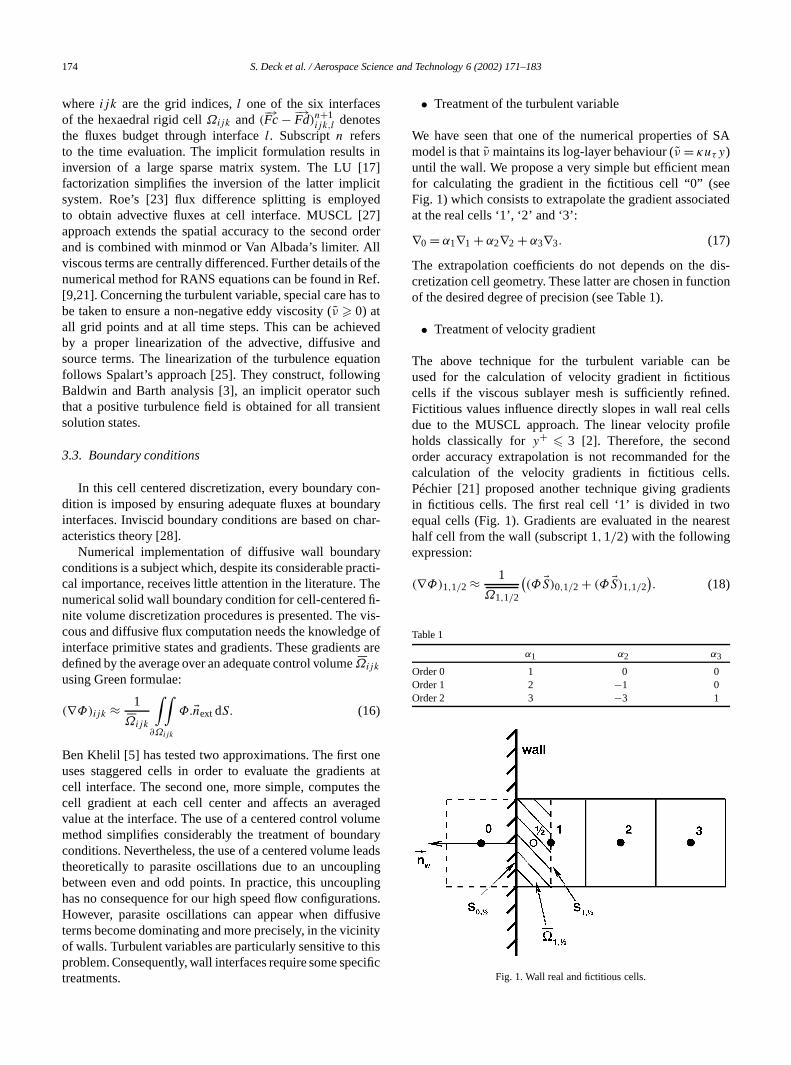
Ben Khelil [5] has tested two approximations. The first oneuses staggered cells in order to evaluate the gradients atcell interface. The second one, more simple, computes thecell gradient at each cell center and affects an averagedvalue at the interface. The use of a centered control volumemethod simplifies considerably the treatment of boundaryconditions. Nevertheless, the use of a centered volume leadstheoretically to parasite oscillations due to an uncouplingbetween even and odd points. In practice, this uncouplinghas no consequence for our high speed flow configurations.However, parasite oscillations can appear when diffusiveterms become dominating and more precisely, in the vicinityof walls. Turbulent variables are particularly sensitive to thisproblem. Consequently, wall interfaces require some specifictreatments.

• Treatment of the turbulent variable

We have seen that one of the numerical properties of SAmodel is thatν maintains its log-layer behaviour (ν = κuτ y)until the wall. We propose a very simple but efficient meanfor calculating the gradient in the fictitious cell “0” (seeFig. 1) which consists to extrapolate the gradient associatedat the real cells ‘1’, ‘2’ and ‘3’:

∇0 = α1∇1 + α2∇2 + α3∇3. (17)

The extrapolation coefficients do not depends on the dis-cretization cell geometry. These latter are chosen in functionof the desired degree of precision (see Table 1).

• Treatment of velocity gradient

The above technique for the turbulent variable can beused for the calculation of velocity gradient in fictitiouscells if the viscous sublayer mesh is sufficiently refined.Fictitious values influence directly slopes in wall real cellsdue to the MUSCL approach. The linear velocity profileholds classically fory+ 3 [2]. Therefore, the secondorder accuracy extrapolation is not recommanded for thecalculation of the velocity gradients in fictitious cells.Péchier [21] proposed another technique giving gradientsin fictitious cells. The first real cell ‘1’ is divided in twoequal cells (Fig. 1). Gradients are evaluated in the nearesthalf cell from the wall (subscript 1,1/2) with the followingexpression:

(∇Φ)1,1/2 ≈ 1

Ω1,1/2

((Φ S)0,1/2 + (Φ S)1,1/2

). (18)

Table 1

α1 α2 α3

Order 0 1 0 0Order 1 2 −1 0Order 2 3 −3 1

Fig. 1. Wall real and fictitious cells.


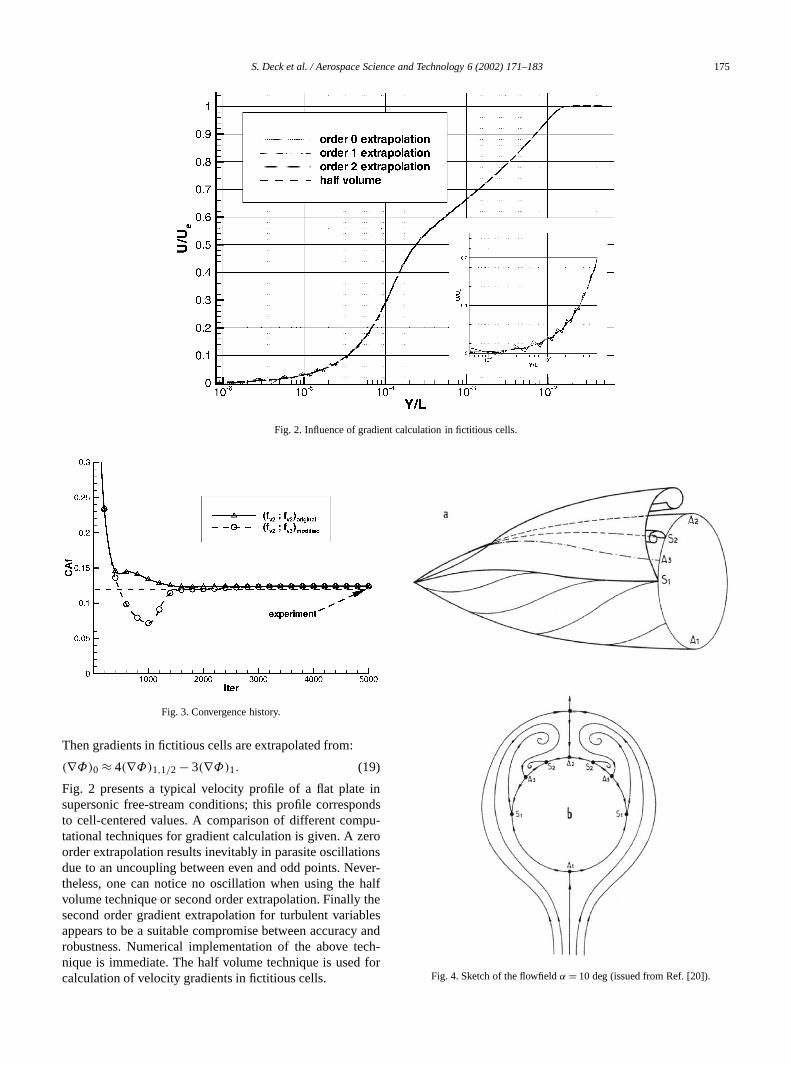
Fig. 2. Influence of gradient calculation in fictitious cells.

Fig. 3. Convergence history.

Then gradients in fictitious cells are extrapolated from:

(∇Φ)0 ≈ 4(∇Φ)1,1/2 − 3(∇Φ)1. (19)

Fig. 2 presents a typical velocity profile of a flat plate insupersonic free-stream conditions; this profile correspondsto cell-centered values. A comparison of different compu-tational techniques for gradient calculation is given. A zeroorder extrapolation results inevitably in parasite oscillationsdue to an uncoupling between even and odd points. Never-theless, one can notice no oscillation when using the halfvolume technique or second order extrapolation. Finally thesecond order gradient extrapolation for turbulent variablesappears to be a suitable compromise between accuracy androbustness. Numerical implementation of the above tech-nique is immediate. The half volume technique is used forcalculation of velocity gradients in fictitious cells. Fig. 4. Sketch of the flowfieldα = 10 deg (issued from Ref. [20]).


Fig. 5. Skin friction contours and separation lines.

4. Results-discussion

4.1. External flows

SA model implemented in FLU3M has been validatedwith various conventional configurations as a part of theSIAM (Simulation Industrielle de l’Aérodynamique desMissiles) program. Two simple but representative test caseshave been chosen for generic configurations at Mach 2 andmoderate angle of attack: a simple circular body and a body-tail configuration.

4.1.1. Ogive-cylinderα = 0A basic study of the influence offv functions is con-

ducted forα = 0 deg. The flow is turbulent (forced transi-tion near the body nose) and Reynolds number based on thediameter is equal to 1.2 106. Fig. 3 presents a typical conver-gence history of the friction drag coefficient (most restrict-ing criterion) together with the experimental value. Modifiedfunctions(fv2, fv3) shifts laminar-turbulent transition back-ward but do not modify the converged value of the normalforce coefficient. Moreover, one can notice a slight differ-ence of speed convergence; the steady state is reached afteronly 1700 iterations with originalfv functions while 3000iterations are necessary to obtain the same value with mod-ified fv functions. Both calculations have been performedwith a CFL number equals to 50.

Fig. 6. Total pressure(pi/pi0) contours in the cross sectionX/D = 7 atα = 10 deg.

4.1.2. Ogive-cylinderα = 10A detailed experimental study of an ogive cylinder

(oil flow visualisations, flowfield measurements, pressuredistributions, boundary layer profiles, skin friction values)


Fig. 7. Eddy viscosity field.

has been carried out at ONERA wind tunnels at Mach 2,particularly at 10 deg of incidence. The flow structure isclassical, including a primary vortex and a secondary one(Fig. 4), but the major interest of this test case is that theintensity of the vortex flow is highly sensitive to the laminaror turbulent nature of the boundary-layers. Indeed, withinthe framework of a GARTEUR group (AG24), this resultswere already used to test and compare a lot of turbulencemodels and codes. Two Reynolds numbers have been underconsideration. First experiments [20] are carried out witha ‘transitional’ Reynolds number ReyD= 0.16 millions(based on the diameter of the cylinder). This allowed toswitch from laminar to turbulent boundary layer when the

transition was free or triggered on the body apex (the natureof the boundary have was controlled by acenaphtene coatingvisualisation). To be sure that the flow is ‘fully turbulent’and also to complete the database, a lot of experiments witha Reynolds number (ReyD= 1.2 millions) were conductedin a second step [14].

Freestream conditions are Mach= 2 and α = 10.Laminar calculations are performed with ReyD= 0.16millions and ReyD= 1.2 millions for all other turbulentcalculations.

The grid, has about 400 000 points (61 in the axialdirection, 85 in the radial direction, 73 in circumferentialdirection with.Φ = 2.5 deg). Moreover, a normal size cell


Fig. 8. Wall pressure coefficient(Cp).

in axial direction (equal to 2.5 10–6 D) leading toY+ < 1 isassumed around the whole body (checked with calculationsatα = 0).

The numerical validation is completed with a K-epsilonmodel computation (Jones and Launder [18]).

Computed skin friction lines are presented on Fig. 5 (de-veloped view). Experimental location of primary and sec-ondary separation lines are obtained from oil flow visualisa-tions. One can notice a good position of the primary separa-tion line is observed with both models, the second separationline is quite visible.

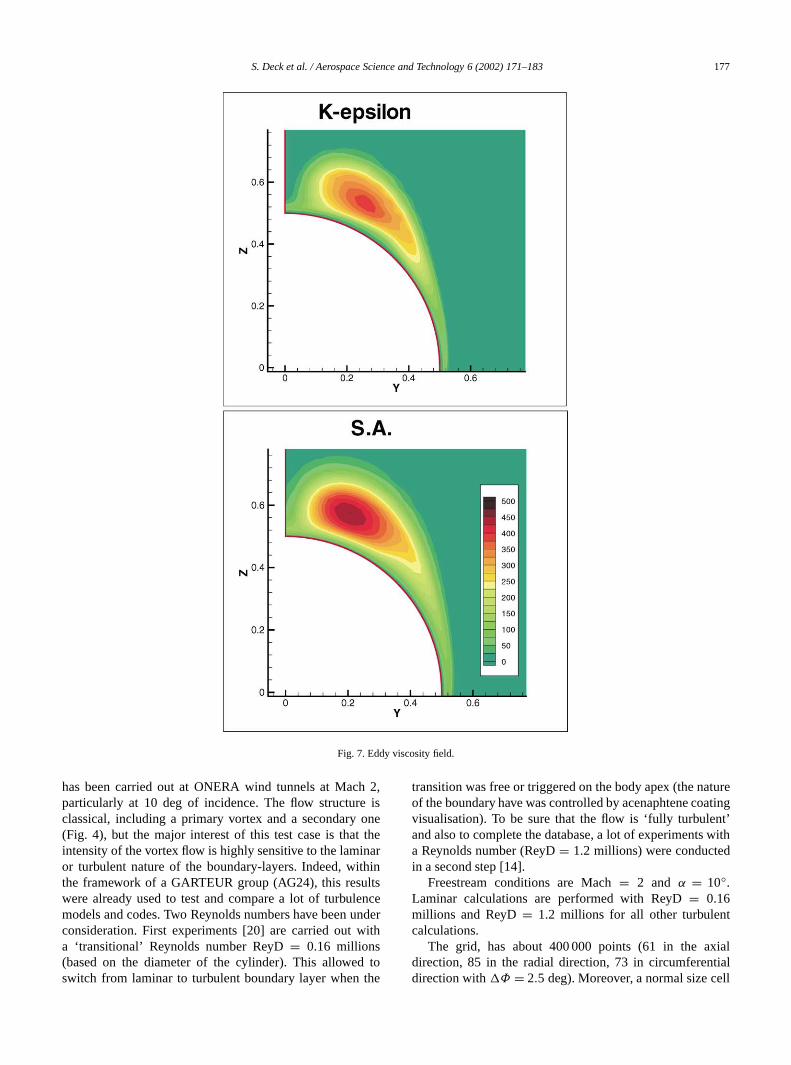
At stationX/D = 7 the main vortex on upper side of thebody shown by total pressure contours of Fig. 6, is alreadydeveloped for this angle of attack. The secondary vortexis embedded in the boundary layer and cannot thereforebe clearly seen. It is wellknown that computational resultsare very sensitive to viscous effects (laminar/turbulent) andto turbulence modelling [14]. Moreover SA and K-epsilongive very close results for total pressure and eddy-viscosity(Fig. 7).

Under the main vortical in leeward side (φ = 140 deg) asuction peak is found on the pressure distributions (Fig. 8).This peak is linked to the high intensity of vortex primarystructure and to wall proximity. K-epsilon, and SA modelsagree with the experiment, except near this peak due to anoverprediction of the eddy viscosity.

The cumulated normal force coefficient obtained by inte-gration of pressure distributions along the body is presentedFig. 9. Euler and laminar calculations are also presented. Thedifferences are clearly related to the vortical lift and eddyviscosity: no vortical lift for Euler calculations, under esti-mation of vortical lift for K-epsilon and SA calculations.

In spite of slight differences in normal force coefficient(CN), both models give the same axial force coefficients(pressure+ skin friction) and compare well with theexperimental results as can be seen on Fig. 10.

Fig. 9. Comparison of the normal force coefficient(CN).

Fig. 10. Total axial force coefficient.

4.1.3. Body-tail configurationThis second test case was considered in order to get an

insight into the effect of vortices on the overall aerodynamicsof a body-fin configuration, and more precisely on theinduced rolling moment. The results presented hereafterwere obtained at Mach 2 and for a non-symmetric roll angleof 22.5. Euler and Spalart–Allmaras solutions are comparedto experiments. Fig. 11 shows the forebody vortices actingon the fins.

The prediction of normal force (Fig. 12) is very good forthe Spalart–Allmaras computation, but not so bad for theinviscid one. This is quite surprising, and can be explainedby the fact that with the inviscid solution the body liftis underestimated (as seen above), whereas the fin lift isoverestimated (no or very small effect of the vortices). Onthe other hand, an accurate estimation of the rolling momentis only obtained by taking into account the viscous effects


Fig. 11. Total pressure contours.

Fig. 12. Normal force coefficient.

(Spalart–Allmaras model on Fig. 13) because it is highlydependent on the individual contribution of each fin.

Generic configurations have been studied for supersonicflow and moderate angles of attack: a body alone and a body-tail. For the body alone a detailed study was performed at10 of incidence. None of the models is really satisfactory:Spalart–Allmaras and K-epsilon (Jones–Launder) give veryclose results between one another but slightly overestimatethe eddy viscosity. TheCN induced by the vortical flowdeveloped on leeward side is very sensitive to viscous effects(laminar/turbulent) and to the turbulence model. However,for configurations with rear tails, body vortical flow haveno tangible effect on the global longitudinal characteristics(CN) as showed by the good agreement obtained with

Fig. 13. Polar in roll fuselage+ wing.

inviscid calculations. Taking into account the vortical bodyis important to predict correctly the rolling moment. Thiswas done with SA model.

4.2. Internal flows

In the frame of ‘JAPHAR’ project, focused on scramjettechnologies and involving DLR and ONERA [19], an in-ternal compression inlet was designed to match the require-ments of a mixed-combustion engine between Mach number4 and 8 [15].


Fig. 14. Isolated inlet in S3MA wind tunnel.

This inlet is supposed to be operated with fixed geome-try on a small scale flight test vehicle propelled by a scram-jet engine burning hydrogen as a fuel. The air flow is de-celerated trough a series of ramps prior to the combustionchamber and, since the compression process is fully inter-nal, four boundary layer bleeds are positioned upstream theinlet throat in order to minimise corner flow developmentsand shock induced boundary layer separations. A contrac-tion ratio around 4 is chosen to decelerate the air flow suf-ficiently at high Mach number while keeping stabilised flowconditions inside the inlet at the lowest bound of the flightrange.

The inlet design is influenced to a great extent by thedesign of the scramjet engine itself. Two struts levels areindeed installed in the combustion chamber for an efficientfuel injection and mixing in the air. Furthermore, sinceignition delays are quite high in supersonic flows, the inletdiffuser must act as scramjet chamber: hence, the struts arepositioned in its upstream part, where only a small amountof divergence is allowed to minimise losses associatedwith supersonic combustion. All these features give theinlet highly three-dimensional characteristics and make itsnumerical simulation a real challenge.

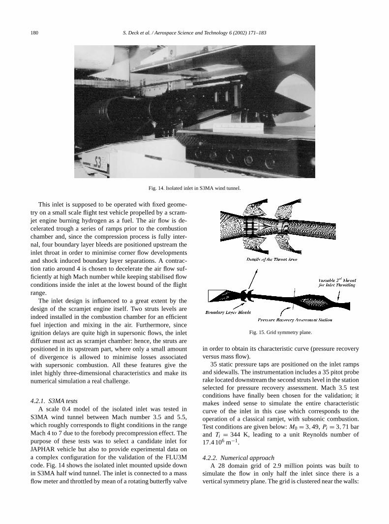
4.2.1. S3MA testsA scale 0.4 model of the isolated inlet was tested in

S3MA wind tunnel between Mach number 3.5 and 5.5,which roughly corresponds to flight conditions in the rangeMach 4 to 7 due to the forebody precompression effect. Thepurpose of these tests was to select a candidate inlet forJAPHAR vehicle but also to provide experimental data ona complex configuration for the validation of the FLU3Mcode. Fig. 14 shows the isolated inlet mounted upside downin S3MA half wind tunnel. The inlet is connected to a massflow meter and throttled by mean of a rotating butterfly valve

Fig. 15. Grid symmetry plane.

in order to obtain its characteristic curve (pressure recoveryversus mass flow).

35 static pressure taps are positioned on the inlet rampsand sidewalls. The instrumentation includes a 35 pitot proberake located downstream the second struts level in the stationselected for pressure recovery assessment. Mach 3.5 testconditions have finally been chosen for the validation; itmakes indeed sense to simulate the entire characteristiccurve of the inlet in this case which corresponds to theoperation of a classical ramjet, with subsonic combustion.Test conditions are given below:M0 = 3,49,Pi = 3,71 barand Ti = 344 K, leading to a unit Reynolds number of17.4 106 m−1.

4.2.2. Numerical approachA 28 domain grid of 2.9 million points was built to

simulate the flow in only half the inlet since there is avertical symmetry plane. The grid is clustered near the walls:


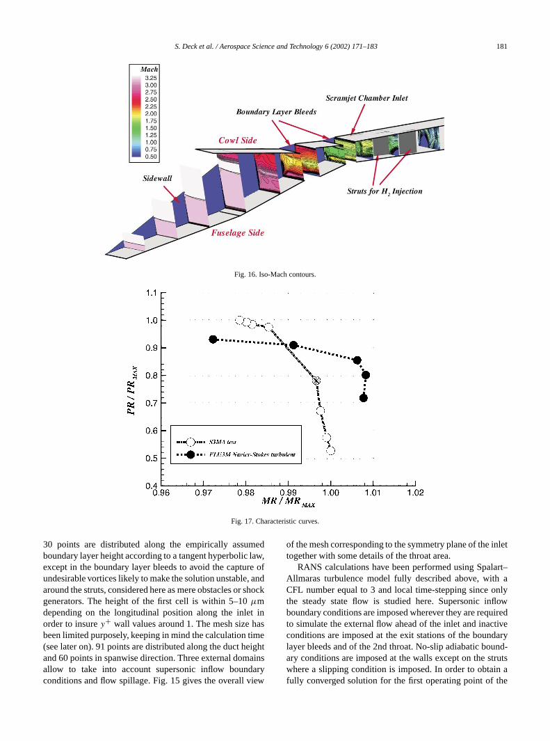
Fig. 16. Iso-Mach contours.

Fig. 17. Characteristic curves.

30 points are distributed along the empirically assumedboundary layer height according to a tangent hyperbolic law,except in the boundary layer bleeds to avoid the capture ofundesirable vortices likely to make the solution unstable, andaround the struts, considered here as mere obstacles or shockgenerators. The height of the first cell is within 5–10µmdepending on the longitudinal position along the inlet inorder to insurey+ wall values around 1. The mesh size hasbeen limited purposely, keeping in mind the calculation time(see later on). 91 points are distributed along the duct heightand 60 points in spanwise direction. Three external domainsallow to take into account supersonic inflow boundaryconditions and flow spillage. Fig. 15 gives the overall view

of the mesh corresponding to the symmetry plane of the inlettogether with some details of the throat area.

RANS calculations have been performed using Spalart–Allmaras turbulence model fully described above, with aCFL number equal to 3 and local time-stepping since onlythe steady state flow is studied here. Supersonic inflowboundary conditions are imposed wherever they are requiredto simulate the external flow ahead of the inlet and inactiveconditions are imposed at the exit stations of the boundarylayer bleeds and of the 2nd throat. No-slip adiabatic bound-ary conditions are imposed at the walls except on the strutswhere a slipping condition is imposed. In order to obtain afully converged solution for the first operating point of the


inlet, starting from a uniform state at Mach 3.5, 35 000 it-erations are necessary, which means roughly 45 h CPU onONERA NEC SX-5 supercomputer. The other points onlyrequire 25 000 iterations to reach convergence, and are ob-tained step by step, closing progressively the 2nd throat.

4.2.3. Results and discussionThe three-dimensionality of the internal flowfield is

highlighted by Fig. 16 showing several iso-Mach slicesdown to the first struts level. In this example, the transitionbetween supersonic and subsonic flow is achieved through acomplex system of shock trains located around the upstreamstruts, which results in large flow distortions in the chamber.

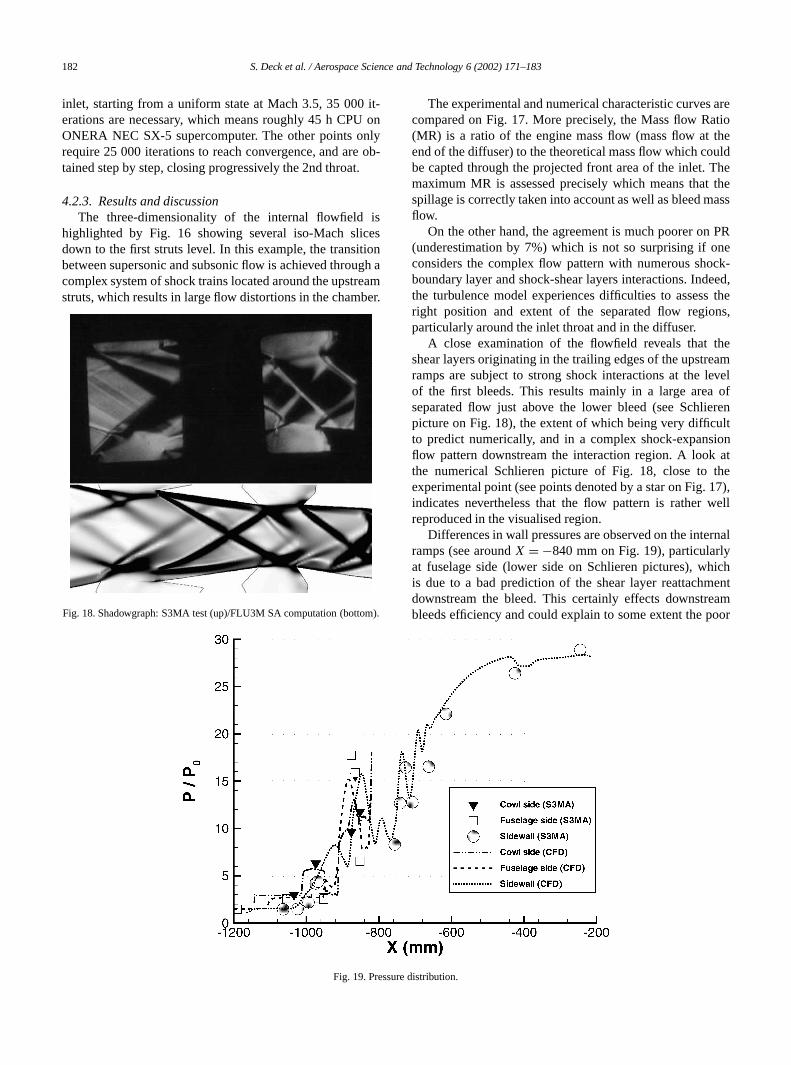
Fig. 18. Shadowgraph: S3MA test (up)/FLU3M SA computation (bottom).

The experimental and numerical characteristic curves arecompared on Fig. 17. More precisely, the Mass flow Ratio(MR) is a ratio of the engine mass flow (mass flow at theend of the diffuser) to the theoretical mass flow which couldbe capted through the projected front area of the inlet. Themaximum MR is assessed precisely which means that thespillage is correctly taken into account as well as bleed massflow.

On the other hand, the agreement is much poorer on PR(underestimation by 7%) which is not so surprising if oneconsiders the complex flow pattern with numerous shock-boundary layer and shock-shear layers interactions. Indeed,the turbulence model experiences difficulties to assess theright position and extent of the separated flow regions,particularly around the inlet throat and in the diffuser.

A close examination of the flowfield reveals that theshear layers originating in the trailing edges of the upstreamramps are subject to strong shock interactions at the levelof the first bleeds. This results mainly in a large area ofseparated flow just above the lower bleed (see Schlierenpicture on Fig. 18), the extent of which being very difficultto predict numerically, and in a complex shock-expansionflow pattern downstream the interaction region. A look atthe numerical Schlieren picture of Fig. 18, close to theexperimental point (see points denoted by a star on Fig. 17),indicates nevertheless that the flow pattern is rather wellreproduced in the visualised region.

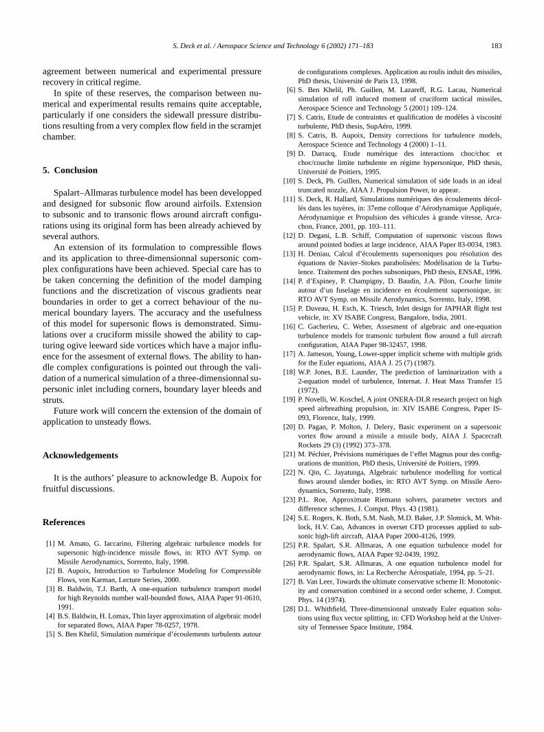
Differences in wall pressures are observed on the internalramps (see aroundX = −840 mm on Fig. 19), particularlyat fuselage side (lower side on Schlieren pictures), whichis due to a bad prediction of the shear layer reattachmentdownstream the bleed. This certainly effects downstreambleeds efficiency and could explain to some extent the poor

Fig. 19. Pressure distribution.


agreement between numerical and experimental pressurerecovery in critical regime.

In spite of these reserves, the comparison between nu-merical and experimental results remains quite acceptable,particularly if one considers the sidewall pressure distribu-tions resulting from a very complex flow field in the scramjetchamber.

5. Conclusion

Spalart–Allmaras turbulence model has been developpedand designed for subsonic flow around airfoils. Extensionto subsonic and to transonic flows around aircraft configu-rations using its original form has been already achieved byseveral authors.

An extension of its formulation to compressible flowsand its application to three-dimensionnal supersonic com-plex configurations have been achieved. Special care has tobe taken concerning the definition of the model dampingfunctions and the discretization of viscous gradients nearboundaries in order to get a correct behaviour of the nu-merical boundary layers. The accuracy and the usefulnessof this model for supersonic flows is demonstrated. Simu-lations over a cruciform missile showed the ability to cap-turing ogive leeward side vortices which have a major influ-ence for the assesment of external flows. The ability to han-dle complex configurations is pointed out through the vali-dation of a numerical simulation of a three-dimensionnal su-personic inlet including corners, boundary layer bleeds andstruts.

Future work will concern the extension of the domain ofapplication to unsteady flows.

Acknowledgements

It is the authors’ pleasure to acknowledge B. Aupoix forfruitful discussions.

References

[1] M. Amato, G. Iaccarino, Filtering algebraic turbulence models forsupersonic high-incidence missile flows, in: RTO AVT Symp. onMissile Aerodynamics, Sorrento, Italy, 1998.

[2] B. Aupoix, Introduction to Turbulence Modeling for CompressibleFlows, von Karman, Lecture Series, 2000.

[3] B. Baldwin, T.J. Barth, A one-equation turbulence transport modelfor high Reynolds number wall-bounded flows, AIAA Paper 91-0610,1991.

[4] B.S. Baldwin, H. Lomax, Thin layer approximation of algebraic modelfor separated flows, AIAA Paper 78-0257, 1978.

[5] S. Ben Khelil, Simulation numérique d’écoulements turbulents autour

de configurations complexes. Application au roulis induit des missiles,PhD thesis, Université de Paris 13, 1998.

[6] S. Ben Khelil, Ph. Guillen, M. Lazareff, R.G. Lacau, Numericalsimulation of roll induced moment of cruciform tactical missiles,Aerospace Science and Technology 5 (2001) 109–124.

[7] S. Catris, Etude de contraintes et qualification de modèles à viscositéturbulente, PhD thesis, SupAéro, 1999.

[8] S. Catris, B. Aupoix, Density corrections for turbulence models,Aerospace Science and Technology 4 (2000) 1–11.

[9] D. Darracq, Etude numérique des interactions choc/choc etchoc/couche limite turbulente en régime hypersonique, PhD thesis,Université de Poitiers, 1995.

[10] S. Deck, Ph. Guillen, Numerical simulation of side loads in an idealtruncated nozzle, AIAA J. Propulsion Power, to appear.

[11] S. Deck, R. Hallard, Simulations numériques des écoulements décol-lés dans les tuyères, in: 37eme colloque d’Aérodynamique Appliquée,Aérodynamique et Propulsion des véhicules à grande vitesse, Arca-chon, France, 2001, pp. 103–111.

[12] D. Degani, L.B. Schiff, Computation of supersonic viscous flowsaround pointed bodies at large incidence, AIAA Paper 83-0034, 1983.

[13] H. Deniau, Calcul d’écoulements supersoniques pou résolution deséquations de Navier–Stokes parabolisées: Modélisation de la Turbu-lence. Traitement des poches subsoniques, PhD thesis, ENSAE, 1996.

[14] P. d’Espiney, P. Champigny, D. Baudin, J.A. Pilon, Couche limiteautour d’un fuselage en incidence en écoulement supersonique, in:RTO AVT Symp. on Missile Aerodynamics, Sorrento, Italy, 1998.

[15] P. Duveau, H. Esch, K. Triesch, Inlet design for JAPHAR flight testvehicle, in: XV ISABE Congress, Bangalore, India, 2001.

[16] C. Gacherieu, C. Weber, Assesment of algebraic and one-equationturbulence models for transonic turbulent flow around a full aircraftconfiguration, AIAA Paper 98-32457, 1998.

[17] A. Jameson, Young, Lower-upper implicit scheme with multiple gridsfor the Euler equations, AIAA J. 25 (7) (1987).

[18] W.P. Jones, B.E. Launder, The prediction of laminarization with a2-equation model of turbulence, Internat. J. Heat Mass Transfer 15(1972).

[19] P. Novelli, W. Koschel, A joint ONERA-DLR research project on highspeed airbreathing propulsion, in: XIV ISABE Congress, Paper IS-093, Florence, Italy, 1999.

[20] D. Pagan, P. Molton, J. Delery, Basic experiment on a supersonicvortex flow around a missile a missile body, AIAA J. SpacecraftRockets 29 (3) (1992) 373–378.

[21] M. Péchier, Prévisions numériques de l’effet Magnus pour des config-urations de munition, PhD thesis, Université de Poitiers, 1999.

[22] N. Qin, C. Jayatunga, Algebraic turbulence modelling for vorticalflows around slender bodies, in: RTO AVT Symp. on Missile Aero-dynamics, Sorrento, Italy, 1998.

[23] P.L. Roe, Approximate Riemann solvers, parameter vectors anddifference schemes, J. Comput. Phys. 43 (1981).

[24] S.E. Rogers, K. Both, S.M. Nash, M.D. Baker, J.P. Slotnick, M. Whit-lock, H.V. Cao, Advances in overset CFD processes applied to sub-sonic high-lift aircraft, AIAA Paper 2000-4126, 1999.

[25] P.R. Spalart, S.R. Allmaras, A one equation turbulence model foraerodynamic flows, AIAA Paper 92-0439, 1992.

[26] P.R. Spalart, S.R. Allmaras, A one equation turbulence model foraerodynamic flows, in: La Recherche Aérospatiale, 1994, pp. 5–21.

[27] B. Van Leer, Towards the ultimate conservative scheme II: Monotonic-ity and conservation combined in a second order scheme, J. Comput.Phys. 14 (1974).

[28] D.L. Whithfield, Three-dimensionnal unsteady Euler equation solu-tions using flux vector splitting, in: CFD Workshop held at the Univer-sity of Tennessee Space Institute, 1984.

Documents

Development and application of Spalart–Allmaras one … and application of Spalart–Allmaras one equation turbulence model to three-dimensional supersonic complex conﬁgurations