Development and Application of CV Benchmarks

Naval Center for Cost AnalysisSCEA Luncheon; 18 May 2011

Brian Flynn

Contents

Development of Benchmarks

• Conjectures

• Data Collection

• Cost Growth Calculations

• MS B Results

• MS C Results

• Other Findings

• Summary of Findings

• Policy Considerations

• Operational Construct

Application of Benchmarks

• Case Study: NATO AGS– Program

– Cost Element Structure

– ICE Methodology

• Point Estimate

– Elements of Risk

– Scenarios

– S-Curve

• S-Curve Tool

• Backup

2

Conjectures of CV Behavior

Conjectures

• Estimation Consistency– CVs from ICEs jibe with acquisition

experience

• Evaluation of accuracy more problematic

• Decline During Acquisition– CVs decrease throughout

acquisition lifecycle

• MS A, B, C, FRP DR

• Platform Homogeneity– CVs equivalent for aircraft, ships,

and other platform types

• Cost growth factors and variances

Conjectures

• Adjustment Decline– CVs decrease when adjusted

for changes in quantity and inflation

• Secular Invariance– CVs steady long-term

3

Data Collection

Source

• SAR Summary Sheets– Total program acquisition cost

• R&D, procurement, MILCON

– Tied to acquisition milestones

• Planning Estimate (PE) for MS A

• Development Estimate (DE) for MS B

• Production Estimate (PdE) for MS C

• Historically, equivalent to milestones I, II, and III

– Base-year$ and then-year$

– From 1985 to 2009

Focus

• DON MDAPS only

• 100 observations

• Baseline Estimates date from 1969 to 2003– Mostly completed programs

but a few on-going such as LPD-17 and LCS

– Ships, submarines, missiles, and aircraft predominate

– Excludes notables such as A-12 and Presidential Helicopter

4

Cost Growth Calculations

Cost Growth Factors (CGFs)

• Unadjusted for quantity changes• Current Estimate in base-year$

divided by Baseline Estimate in base-year$

• Adjusted for changes in inflation

• Current Estimate in then-year$ divided by Baseline Estimate in then-year$

• Completely unadjusted

• Adjusted for quantity changes• Also in base-year and then-year$

Quantity Adjustment

• Three choices– Adjust baseline estimate to

reflect current quantities

• CGF = CE/(BE + Q∆)

• Analogous to Paasche Index

• Used in SARs

– Adjust current estimate to reflect baseline quantities

• CGF = (CE – Q∆)/BE

• Analogous to Laspeyres Index

– “Fischer” index = square root of the product of the first two

• CV deltas insignificant (.02 and .04

spreads in BY$ & TY$ for ships & submarines) 5

Cost Growth Calculations

Example: CG-47 Class

6

• Baseline Estimate (BE) of 1978

– 16 ships at $9.01B (BY$) and $14.08B (TY$)

• Current Estimate (CE) of 1992

– 27 ships at $14.11B (BY$) and $23.28B (TY$)

• Deltas in BY$

• $5.10B total & $5.49B quantity

• Deltas in TY$

• $9.20B total & $11.74B quantity

• Estimating change negative

• Unadjusted for quantity ∆– Then-year dollars

$23.28B/$14.08B = 1.65

– Base-year dollars

$14.11B/$9.01B = 1.57

• Adjusted for quantity ∆, using OSD methodology – Then-year dollars

$23.28B/($14.08B + $11.74B ) = 0.90

– Base-year dollars

$14,11B /($9.01B + $5.49B) = 0.97

Cost Growth Factors

Provenance of Baseline Estimates

7

Ratio of Ratio of Ratio of Ratio of

POACE to POACE to ICE to ICE to

SAR BE SAR BE SAR BE SAR BE

in BY$ in TY$ in BY$ in TY$ in BY$ in TY$ in BY$ in TY$ in BY$ in TY$

$2,877 $3,093 $2,817 $3,032 $3,130 0.98 0.98 1.09

$4,123 $4,310 $4,123 $4,104 1.00 1.00

$45,633 $71,081 $45,500 $47,400 1.00 1.04

$8,636 $8,400 $8,580 0.97 0.99

$26,494 $31,429 $24,490 $26,810 0.92 1.01

$31,548 $36,296 $32,800 $39,100 1.04 1.24

$10,627 $11,425 $10,727 1.01

$43,490 $46,826 $43,000 0.99

$4,263 $4,890 $4,245 $4,349 1.00 1.02

$2,977 $3,290 $3,019 $3,284 $3,505 1.01 1.00 1.07

Means = 0.99 0.98 1.07 1.03

1.03 without outlier

Program Office's

Acquisition ICE (CAIG for ID;

SAR BE Cost Estimate NCCA for IC)

Analysis of Deltas

Comparisons based on available data for cost estimates of recent vintage (1990 and later)

• 6 ACAT ID programs (OSD CAIG ICE)

• 4 ACAT IC programs (NCCA ICE)

F/A-18 E/F

JSOW

Expeditionary Fighting Vehicle (formerly AAAV)

MIDS - Low Volumne Terminal (LVT)

Cooperative Engagement Capability (CEC)

H-1 UPGRADES

MH-60S

TACTICAL TOMAHAWK

MH-60R

E-2D Advanced Hawkeye

EA-18G (Electronic Attack - 18G Growler)

COBRA JUDY REPLACEMENT

P-8A

Mobile User Objective System (MOUS)

SM-6

AGM-88E AARGM

Sample Data at MS B

Database Elements• Base year, baseline

type, platform type• Baseline Estimate

– Base Year$– Then Year$– Quantity

• Changes to Date– Base Year$– Then Year$– Quantity

• Current Estimate– Base Year$– Then Year$– Quantity

• Quantity Changes– Base Year$ – Then Year $

• Date of last SAR

8

F-14D

F/A-18 C/D

Fixed Distributed System (FDS)

HARM

HARPOON

LAMPS MK III

MK-48 ADCAP

MK-50 TORPEDO

PHOENIX AIM-54C

SEA LANCE (ASW-SOW)

SH-60F

SPARROW (AIM-7M)

STANDARD MISSILE-2 (Blocks I to IV)

TOMAHAWK Baseline Improvement Program (TBIP)

V-22

AN/BSY-2

SLAT (Supersonic Low Altitude Target)

DDG-51 Destroyers (Arleigh Burke Class)

DDG-1000 Destroyers (Zumwalt Class)

CVN-78 Aircraft Carriers (Gerald R. Ford Class)

LPD-17 Amphibious Transport Dock (San Antonio Class)

LHA-6 Amphibious Assault Ships (America Class)

SSN-774 Attack Submarines (Virginia Class)

LHD-1

CG-47

SSN-688 Submarines

Strategic Sealift

FFG-7

AN/BSY-1 (Submarine Advanced Combat System; SUBACS)

Airborne Self Protection Jammer (ASPJ)

AV-8B

C/MH-53E

E-6A

F-14A

n = 50

MS B: All Programs

All DON MDAPs at MS B• Distribution skewed to

right

• Adjustments for changes in quantity and inflation decrease values of CGFs and CVs

• CVs sensitive to outliers– E.g., removing

Harpoon decreases quantity-adjusted TY$ CV to 0.45

• 2nd oldest datum (1970 baseline)

9

0

2

4

6

8

10

12

14

16

18

< 0.75 0.75 - 1.00 1.01 - 1.25 1.26 - 1.50 1.51 - 1.75 1.76 - 2.00 2.01 - 2.25 2.26 - 2.50 2.51 - 2.75 >= 2.76

Fre

qu

en

cy

Cost Growth Factor (Current Estimte/Baseline Estimate)

Acquisition Cost Growth from MS B for "All" DON MDAPS(Quantity Adjusted in Then-Year Dollars)

Median CGF = 1.18

Mean CGF = 1.36CV = 51%

Base-Year$ Then-Year$ Base-Year$ Then-Year$

Mean 1.48 1.84 1.23 1.36

Standard Deviation 0.94 1.60 0.44 0.69

CV 0.63 0.87 0.36 0.51

(Without Qty Adjustment) (Quantity Adjusted)

Statistics

Cost Growth Factors & CVs for All DON MDAPs at MS B for 1969 & Later; n = 50

MS B: Ships and Submarines

Comparison with “All DON”• Median CGF = (1.18, 1.12)

• Mean CGF = (1.36, 1.30)

• CV = (51%, 45%)

10

Base-Year$ Then-Year$ Base-Year$ Then-Year$

Mean 1.78 2.17 1.21 1.30

Standard Deviation 0.95 1.38 0.30 0.58

CV 0.54 0.64 0.25 0.45

(Without Qty Adjustment) (Quantity Adjusted)

Statistics

Cost Growth Factors & CVs for Ship & Sub MDAPs at MS B; n = 11

0

1

2

3

4

5

0.75 - 1.00 1.01 - 1.25 1.26 - 1.50 1.51 - 1.75 1.76 - 2.00 2.01 - 2.25 2.26 - 2.50 2.51 - 2.75

Fre

qu

en

cy

Cost Growth Factor (Current Estimte/Baseline Estimate)

Acquisition Cost Growth from MS B for Ships & Submarines(Quantity Adjusted in Then-Year Dollars)

Median CGF = 1.12Mean CGF = 1.30

CV = 45%

CG-47 ClassStrategic Sealift

LHD-1 Class

LHA-6 ClassCVN-78 Class

SSN-688 Class

DDG-1000 Class

DDG-51 ClassSSN-774 Class LPD-17 Class FFG-7 Class

SampleMedian Sample Mean

MS B: Aircraft

Comparison with All DON, Ships

• Median CGF = (1.18, 1.12, 1.19)

• Mean CGF = (1.36, 1.30, 1.43)

• CV = (51%, 45%, 44%)

11

0

1

2

3

4

5

6

< 0.75 0.75 - 1.00 1.01 - 1.25 1.26 - 1.50 1.51 - 1.75 1.76 - 2.00 2.01 - 2.25 2.26 - 2.50 2.51 - 2.75 >= 2.76

Fre

qu

en

cy

Cost Growth Factor (Current Estimte/Baseline Estimate)

Acquisition Cost Growth from MS B for Aircraft(Quantity Adjusted in Then-Year Dollars)

F/A-18 C/D

Sample Mean

Median CGF = 1.19

Mean CGF = 1.43CV = 44%

F-14D

AV-8BF-14ASH-60FE-2DEA-18GP-8A

E-6AF/A-18 E/F V-22

SH-60BMH-60SMH-60R

C/MH 53EH-1 Upgrades

SampleMedian

Base-Year$ Then-Year$ Base-Year$ Then-Year$

Mean 1.55 2.03 1.29 1.43

Standard Deviation 0.89 1.87 0.43 0.63

CV 0.57 0.92 0.34 0.44

(Without Qty Adjustment) (Quantity Adjusted)

Statistics

Cost Growth Factors & CVs for Aircraft MDAPs at MS B; n = 16

0

1

2

3

4

5

< 0.75 0.75 - 1.00 1.01 - 1.25 1.26 - 1.50 1.51 - 1.75 1.76 - 2.00 2.01 - 2.25 2.26 - 2.50 2.51 - 2.75 >= 2.76

Fre

qu

en

cy

Cost Growth Factor (Current Estimte/Baseline Estimate)

Acquisition Cost Growth at MS B for Missiles(Quantity Adjusted in Then-Year Dollars)

Median CGF = 1.19

Mean CGF = 1.37CV = 70%

SampleMedian

Sample Mean

Sea LanceTomahawk (TBIP)Phoenix

SLAT

JSOWSM-6AARGM

SM-2

Tactical TomahawkSparrow

HARM Harpoon

MS B: Missiles

Comparison with All DON, Ships, Aircraft• Median CGF = (1.18, 1.12, 1.19, 1.19)

• Mean CGF = (1.36, 1.30, 1.43, 1.37)

• CV = (51%, 45%, 44%, 70%)

12

Without HARPOON

(CGF = 3.96), CV =

47%

Base-Year$ Then-Year$ Base-Year$ Then-Year$

Mean 1.44 1.94 1.19 1.37

Standard Deviation 1.19 1.93 0.49 0.96

CV 0.82 0.99 0.41 0.70

(Without Qty Adjustment) (Quantity Adjusted)

Statistics

Cost Growth Factors & CVs for Missile MDAPs at MS B; n = 12

MS B: Electronics & Other

Comparison with All DON, Ships, Aircraft, Missiles• Median CGF = (1.18, 1.12, 1.19, 1.19, 1.19)

• Mean CGF = (1.36, 1.30, 1.43, 1.37, 1.29)

• CV = (51%, 45%, 44%, 70%, 47%)

13

0

1

2

3

4

5

< 0.75 0.75 - 1.00 1.01 - 1.25 1.26 - 1.50 1.51 - 1.75 1.76 - 2.00 2.01 - 2.25 2.26 - 2.50 2.51 - 2.75 >= 2.76

Fre

qu

en

cy

Cost Growth Factor (Current Estimte/Baseline Estimate)

Acquisition Cost Growth at MS B for Electronics & Other(Quantity Adjusted in Then-Year Dollars)

Median CGF = 1.19

Mean CGF = 1.29CV = 47%

BSY-1 SUBACSFixed Distributed

System

BSY-2MUOSMIDS LVTCOBRA JUDY

MK-48 ADCAPMK-50 TorpedoCEC

ASPJExpeditionary Fighting

Vehicle

SampleMedian

Sample Mean

Base-Year$ Then-Year$ Base-Year$ Then-Year$

Mean 1.14 1.14 1.22 1.29

Standard Deviation 0.67 0.69 0.55 0.60

CV 0.59 0.61 0.45 0.47

(Without Qty Adjustment) (Quantity Adjusted)

Statistics

Cost Growth Factors & CVs for Electronics & Other MDAPs at MS B; n = 11

Hypothesis Testing for MS B

Hypothesis

• Homogeneity of CGF means• Ho: μ1 = μ2 = … = μk, where μi is

a platform population mean CGF

• Ha: μi ≠ μj, for at least one (i,j) pair

• F(3,45) = 0.12 (from ANOVA)

Implies that variation in platform-level sample means is not, at the 5% level of significance, statistically distinguishable from noise

14

1.30 1.43 1.37 1.29

0.0

0.5

1.0

1.5

2.0

2.5

3.0

3.5

4.0

4.5

Ships & Subs Aircraft Missiles Elex & Other

Co

st G

row

th F

acto

r

Means & Spreads of CGFs from MS B(Quantity Adjusted in Then-Year$)

Sample σ2 = .34

Sample σ2 = .40

Sample σ2 = .92

Sample σ2 = .36

Hypothesis Testing for MS B

Hypothesis

• Homogeneity of CGF variances Ho: σ2

1 = σ2

2 = … = σ2

k, where σ2i is a

platform population variance CGF

Ha: σ2

i ≠ σ2

j , for at least one (i,j) pair

Statistical tests:

Pairwise comparisons

Levene test for k samples

Test Results

• Pairwise comparisons– In all cases, Ho is not rejected

at 5% level of significance

• Levene’s test For skewed distributions

F(3,47) = 0.46 versus critical value of 4.23; Ho not rejected

• In both cases, platform-level sample variances not statistically distinguishable from noise

15

Ships & Elex &

Platforms Subs Aircraft Missiles Other

Ships and Subs 2.840 2.940 2.970

Aircraft 2.510 2.720

Missiles 2.940

Elex and Other

Sample Pairwise F Statistics

Homogeneous means and variances strongly support the conjecture of homogeneous CVs

Other Findings for MS B

• CVs decline monotonically with adjustments– 15 percentage points for inflation, after quantity adjustment

• Perhaps due to volatility of average annual rates during the Nixon/Ford (6.5%), Carter (10.7%), Reagan (4.0%), G.H.W. Bush (3.9%), and Clinton (2.7%) administrations

16

0.87

0.63

0.51

0.36

0

0.2

0.4

0.6

0.8

1

Then-Year$ Base-Year$ Then-Year$ Base-Year$

Co

eff

icie

nts

of

Var

iati

on

Quantity- and Inflation-Adjusted CVs from MS B

Quantity Unadjusted

Aircraft

Electronics

Missiles

Ships

Quantity Adjusted

51 and 15percentage points of CV

Other Findings for MS B

Secular decline in CVs

• Especially in TY$– Less drop in BY$

• Inflation stability– After the turmoil of

the late 1970s

• Less variance and greater accuracy in OMB rates

• Less CV (TY$ to BY$)

– Unclear if trend will continue in long run

• Caution:– Confidence lessens as

sample size decreases

17

0

0.2

0.4

0.6

0.8

1

Then-Year$ Base-Year$ Then-Year$ Base-Year$

Co

eff

icie

nts

of

Var

iati

on

Secular Trends in CVs from MS B

Quantity Unadjusted

=> 1980; n = 37

=> 1990; n = 22

24 percentage points of CV

Quantity Adjusted

15 percentage points of CV

=> 1969; n = 50

Sample Data at MS C

All DON MDAPs at MS C

18

n = 43

• PdE represents estimated total program acquisition cost• Includes sunk R&D

and MILCON costs

• Roughly 20% had a DE, too

DDG-51 Destroyers (Arleigh Burke Class)

CVN-77 (1 ship) from CVN-68 Aircraft Carriers (Nimitz Class)

T-AKE Dry Cargo/Ammunition Ships (Lewis and Clark Class)

AOE-6

CVN-72/73

CVN-74/75

Landing Craft Air Cushion (LCAC) Vehicles

LSD-41 Landing Ship Dock (Whidbey Island Class)

LSD-49 Landing Ship Dock (Cargo Variant)

MCM-1 Mine Countermeasure Ships (Avenger Class)

TAO-187 Fleet Oiler

Trident II Submarines

CVN-76

MHC-51 Mine Hunter Coastal Class Ships

T-AGOS

CVN-68 Class (two ships)

CVN-68 Class (one ship)

Battleship Reactivation

SSN-21 & AN/BSY-2

A-6E/F

AN/SQQ-89 Anti-Submarine Warfare System

E-2C

EA-6B

F-14D

MK-48 ADCAP

P-3C

PHALANX CIWS

T-45TS

TRIDENT II MISSILE

V-22

UHF FOLLOW-ON

ROTHR (Relocatable Over the Horizon Radar)

F/A-18 E/F

JSOW Baseline/Unitary-108

MIDS - Low Volumne Terminal (LVT)

Navy EHF Satellite Communications Program (NESP)

AV-8B REMANUFACTURE

Cooperative Engagement Capability (CEC)

E-2C REPRODUCTION

MH-60S

TACTICAL TOMAHAWK

MH-60R

EA-18G (Electronic Attack - 18G Growler)

MS C: All Programs

All DON MDAPs at MS C• CVs uniformly lower

• Cost growth factors less compared to DE values

– Mean (1.10 versus 1.36)

– Median (1.07 versus 1.18)

– Similar trend for the 9 programs with both DEs and PdEs

• Distribution less skewed

19

0

5

10

15

20

25

< 0.75 0.75 - 1.00 1.01 - 1.25 1.26 - 1.50 1.51 - 1.75 1.76 - 2.00 2.01 - 2.25 2.26 - 2.50 2.51 - 2.75 >= 2.76

Fre

qu

en

cy

Cost Growth Factor (Current Estimte/Baseline Estimate)

Acquisition Cost Growth from MS C for "All" DON MDAPS(Quantity Adjusted in Then-Year Dollars)

Median CGF = 1.07

Mean CGF = 1.10CV = 26%

Base-Year$ Then-Year$ Base-Year$ Then-Year$

Mean 1.11 1.08 1.11 1.10

Standard Deviation 0.50 0.58 0.21 0.28

CV 0.45 0.53 0.19 0.26

(Without Qty Adjustment) (Quantity Adjusted)

Statistics

Cost Growth Factors & CVs for All DON MDAPs at MS C for 1969 & Later; n = 43

0.87

0.63

0.51

0.36

0.530.45

0.260.19

0

0.2

0.4

0.6

0.8

1

Then-Year$ Base-Year$ Then-Year$ Base-Year$

Co

eff

icie

nts

of

Var

iati

on

CVs for Total Acquisition Cost: MS B and MS C

Quantity Unadjusted

CVs from MS C

Quantity Adjusted

CVs from MS B

MS C: Ships and Submarines

Comparison with “All DON”• Median CGF = (1.07, 1.05)

• Mean CGF = (1.10, 1.07)

• CV = (26%, 22%)

20

0

2

4

6

8

10

< 0.75 0.75 - 1.00 1.01 - 1.25 1.26 - 1.50 1.51 - 1.75 1.76 - 2.00 2.01 - 2.25

Fre

qu

en

cy

Cost Growth Factor (Current Estimte/Baseline Estimate)

Acquisition Cost Growth from MS C for Ships & Submarines(Quantity Adjusted in Then-Year Dollars)

Trident II Subs

Median CGF = 1.05Mean CGF = 1.07

CV = 22%

CVN-72/73LSD-41 ClassLSD-49 ClassTAO-187 ClassLCACsBattleship React

CVN-71 (1 Ship)T-AKE ClassCVN-74/75

MCM-1 ClassCVN-76 (1 Ship)MHC-51 ClassT-AGOSCVN-68 Class (2 ships)

CVN-68 Class (1 ship)

DDG-51 ClassAOE-6 Class

SSN-21 & AN/BSY-2Sample Median and Mean

Base-Year$ Then-Year$ Base-Year$ Then-Year$

Mean 1.15 1.12 1.11 1.07

Standard Deviation 0.59 0.74 0.15 0.24

CV 0.52 0.66 0.14 0.22

(Without Qty Adjustment) (Quantity Adjusted)

Statistics

Cost Growth Factors & CVs for Ship & Sub MDAPs at MS C; n = 19

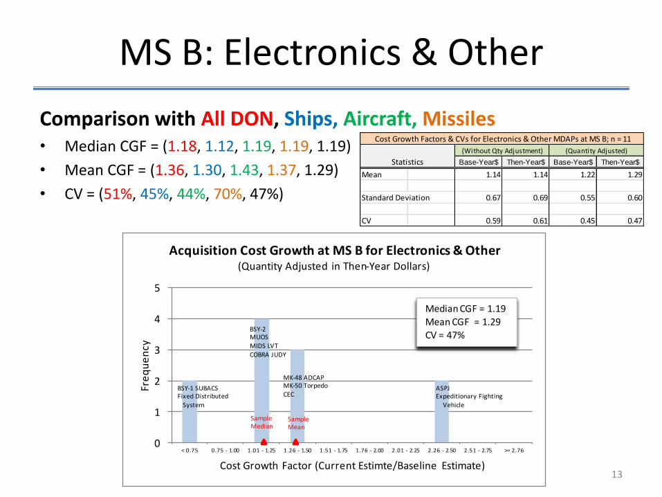
MS C: AircraftComparison with All DON, Ships

• Median CGF = (1.07, 1.05, 1.08)

• Mean CGF = (1.10, 1.07, 1.12)

• CV = (26%, 22%, 36%)

21

Base-Year$ Then-Year$ Base-Year$ Then-Year$

Mean 1.17 1.08 1.15 1.12

Standard Deviation 0.44 0.39 0.31 0.40

CV 0.38 0.36 0.27 0.36

(Without Qty Adjustment) (Quantity Adjusted)

Statistics

Cost Growth Factors & CVs for Aircraft MDAPs at MS C; n = 13

0

2

4

6

8

10

< 0.75 0.75 - 1.00 1.01 - 1.25 1.26 - 1.50 1.51 - 1.75 1.76 - 2.00 2.01 - 2.25

Fre

qu

en

cy

Cost Growth Factor (Current Estimte/Baseline Estimate)

Acquisition Cost Growth from MS C for Aircraft(Quantity Adjusted in Then-Year Dollars)

F-14DP-3C

Median CGF = 1.08Mean CGF = 1.12

CV = 36%

V-22AV-8B Remanufacture

E-2CT-45 TSF/A-18 E/FE-2C Reproduction

MH-60SMH-60R

EA-18G

A-6E/F EA-6BSample Median and Mean

CV falls to

22% without

EA-6B outlier

MS C: “Other”Comparison with All DON, Ships, Aircraft

• Median CGF = (1.07, 1.05, 1.08, 1.12 )

• Mean CGF = (1.10, 1.07, 1.12, 1.12)

• CV = (26%, 22%, 36%, 16%)

22

CV falls to

22% without

EA-6B outlier

0

2

4

6

8

10

< 0.75 0.75 - 1.00 1.01 - 1.25 1.26 - 1.50 1.51 - 1.75 1.76 - 2.00 2.01 - 2.25

Fre

qu

en

cy

Cost Growth Factor (Current Estimte/Baseline Estimate)

Acquisition Cost Growth from MS C for "Other"(Quantity Adjusted in Then-Year Dollars)

Median CGF = 1.12Mean CGF = 1.12

CV = 16%

ROTHRNavy EHF Satellite

AN/SQQ-89MK-48 ADCAP

PHALANX CIWSUHF Follow-OnJSOW Baseline/UnitaryMIDSCooperative Engagement Capability

Trident II MissileTactical Tomahwak

Sample Median and Mean

Base-Year$ Then-Year$ Base-Year$ Then-Year$

Mean 0.99 1.00 1.07 1.12

Standard Deviation 0.39 0.45 0.16 0.18

CV 0.40 0.45 0.15 0.16

(Without Qty Adjustment) (Quantity Adjusted)

Statistics

Cost Growth Factors & CVs for "Other" MDAPs at MS C; n = 11

Insufficient sample sizes for missiles and electronics

Hypothesis Testing for MS C

Hypothesis

• Homogeneity of CGF means• Ho: μ1 = μ2 = … = μk, where μi is

a platform population mean CGF

• Ha: μi ≠ μj, for at least one (i,j) pair

• F(2,40) = 0.16 (from ANOVA)

Implies that variation in platform-level sample means is not, at the 5% level of significance, statistically distinguishable from noise

23

1.07 1.12 1.12

0.0

0.5

1.0

1.5

2.0

2.5

3.0

Ships & Subs Aircraft Other

Co

st G

row

th F

acto

r

Means & Spreads of CGFs from MS C(Quantity Adjusted in Then-Year$)

Sample σ2 = .06

Sample σ2 = .16

Sample σ2 = .03

Hypothesis Testing for MS C

Hypothesis

• Homogeneity of CGF variances Ho: σ2

1 = σ2

2 = … = σ2

k, where σ2i is a

platform population variance CGF

Ha: σ2

i ≠ σ2

j , for at least one (i,j) pair

Statistical tests:

Pairwise comparisons

Levene test for k samples

Test Results

• Mixed– Pairwise comparisons

• Ho rejected for aircraft/ships and aircraft/other

– Due solely to EA-6B outlier

– Levene’s test

For skewed distributions

F(2,38) = 0.54 versus critical value of 3.25; Ho not rejected

– On balance, deltas in sample variances not distinguishable from noise

24

Homogeneous means and some evidence of homogeneous

variances support the conjecture of homogeneous CVs

Ships &

Platforms Subs Aircraft Other

Ships and Subs 2.792 1.677

Aircraft 4.682

Other

Sample Pairwise F Statistics

Other Findings for MS C

Secular decline in CVs

• In both TY$ and BY$– Compared to MS B

results:

• Fewer older programs

• Less inflation impact

• Hypotheses– Better estimating

– Increased program stability

– Stronger link to ICEs

• Caution: confidence lessens as sample size decreases

25

0.00

0.10

0.20

0.30

0.40

0.50

0.60

Then-Year$ Base-Year$ Then-Year$ Base-Year$

Co

eff

icie

nts

of

Var

iati

on

Secular Trends in CVs from MS C

Quantity Unadjusted

=> 1990; n = 20

8 percentage points of CV versus4 points for 1990s & later

Quantity Adjusted

1978 (1 datum) & => 1980s; n = 43

Other Findings: MS A

CVs at MS A

• Insufficient sample size for sound inferences– CV of 49% (TYS; quantity-adjusted)

– Median CGF of 1.65

• Alternative– Use MS B-to-C delta as

analogy to MS A-to-B delta

• Assumes equal degree of cost uncertainty and risk between milestones

– For equal sample time periods, delta ~ 15 percentage points in CV

26

0.00

0.10

0.20

0.30

0.40

0.50

0.60

0.70

0.80

Then-Year$ Base-Year$ Then-Year$ Base-Year$

Co

eff

icie

nts

of

Var

iati

on

Deltas in CVs from MS B to MS C

Quantity Unadjusted

MS B; => 1980s

MS B; => 1990s

MS C; => 1980s

MS C; => 1990s

17 percentage pts

14 percentage pts

Quantity Adjusted

0

1

2

3

< 0.75 0.75 - 1.00 1.01 - 1.25 1.26 - 1.50 1.51 - 1.75 1.76 - 2.00 2.01 - 2.25 2.26 - 2.50 2.51 - 2.75 >= 2.76

Fre

qu

en

cy

Cost Growth Factor (Current Estimte/Baseline Estimate)

Cost Growth Factors at MS A for 7 DON MDAPS(Quantity Adjusted in Then-Year Dollars)

Summary of Findings

Conjectures

• Estimation Consistency– CVs from ICEs jibe with acquisition

experience

• Ad hoc observation suggests underestimation of CVs, at times, in the international defense community

• Decline During Acquisition– CVs decrease throughout acquisition

lifecycle

• Strongly supported (MS B to MS C)

• Platform Homogeneity– CVs equivalent for aircraft, ships, and

other platform types

• Strongly supported, especially for MS B

Conjectures

• Adjustment Decline– CVs decrease when adjusted

for changes in quantity and inflation

• Strongly supported

• Secular Invariance– CVs steady long-term

• Rejected

• Evidence of secular decline

• However, small sample sizes lessen confidence

27

Policy Considerations

General

• Type of CV to employ– Perhaps quantity adjusted in TY$ is

best

• Many programs using non-OSD inflation rates

• Quantity deltas influenced by JCIDS and Congress

• Possibility of structural change– For example,

• WSARA; systems engineering early on; competitive prototyping; affordability as a KPP; should-cost studies; budgeting to SCPs; capability/cost tradeoffs

– Uncertain effect on CGFs & CVs

Benchmark CVs• View of long-term inflation

– Instability would argue for inclusion of data from 1970s

– Stability would argue against

28

Operational Construct

29

1.2

0.80.8

0.5

0.9

0.6

0.5

0.4

0.50.5

0.30.2

0.8 0.8

0.5 0.5 0.5 0.5

0.3 0.3 0.30.3

0.20.10.0

0.2

0.4

0.6

0.8

1.0

1.2

1.4

MS A MS B MS C

Co

eff

icie

nt o

f V

aria

tio

n

Quantity random

TY$ BY$

Quantity random

TY$ BY$

Quantity ExogenousTY$ BY$

Quantity ExogenousTY$ BY$

Quantity ExogenousTY$ BY$

All data Data => 80s Data => 90s

Quantity random

TY$ BY$

Milestone A: Milestone B Milestone CEstimated by analogy

Options for “trigger values” requiring an explanation

• Use historical range

• Use fixed percentage from endpoints

• Use confidence intervals

Operational Construct

Confidence Intervals

• Assumptions– Lognormal distribution

at MS B

– Normal distribution at MS C

• Data from 1980s and later– Other confidence

intervals available

• E.g., MS B, using all sample data

• 0.42, 0.51, 0.66 for lower bound, mean, and upper bound

30

0.74

0.54

0.34

0.41

0.31

0.21

0.0

0.1

0.2

0.3

0.4

0.5

0.6

0.7

0.8

0.9

MS A MS B MS C

Co

eff

icie

nt o

f V

aria

tio

n

95% Confidence Intervals for CVs(Quantity-Adjusted; TY$; Data => 1980s)

Estimated from historical data

Estimated by analogy

Case Study #1

NATO Alliance Ground Surveillance System

31

NATO AGS Program

32

ICE Methodology

Based on DON Cost Estimating Guide

33

Buy-in from NATO, OSD(CAPE), USD(AT&L),

AGS Board of Directors, and “Program Office”;

formal ICE development plan with signatures

Site visits to

NATO AGS

Management

Agency and

Northrop

Grumman

NATO’s

SAS-076

Task

Group

January 2011 meeting in

Brussels

eSBM

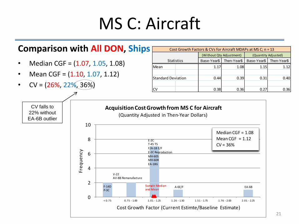
Cost Element Structure

34

ICE Methodology

Unadjusted Point Estimate

• Air Vehicle– Global Hawk Block 30 and 40

actuals

• Learning curves

• Averages

• Payload (MP RTIP)– Analogy to AESA

• Ground Segment– Analogies for hardware

– CERs for software development

• Manmonths

• Burdened salaries from Eurohawk

Unadjusted Point Estimate

• Support Elements– Global Hawk actuals

• G&A, FCCM, & Fee– Global Hawk actuals

35

Notional Quantity Profile

• NATO AGS’s position on learning curve influenced by– U.S. Global Hawk production

– BAMS development and production

36

Cumulative Block 30 & 40 Air Vehicles

0

10

20

30

40

50

60

FY05 FY06 FY07 FY08 FY09 FY10 FY11 FY12 FY13

Year

Cu

mu

lati

ve Q

uan

tity

Includes 2 AGS Qual Units

Includes 6 AGS Production Units

Buy Year; TOA Funding FY02 FY03 FY04 FY05 FY06 FY07 FY08 FY09 FY10 FY11 FY12 FY13

U.S. Global Hawk LRIP Lot 1 Lot 2 Lot 3 Lot 4 Lot 5 Lot 6 Lot 7 Lot 8 Lot 9 Lot 10 Lot 11 Lot 12

Block 10 Aircraft 3 3 1

Block 20 Aircraft 3 3

Block 30 Aircraft 1 4 5 2 2 2 2 3 3

Block 40 Aircraft 1 3 3 2 2 2 2

Total

DON BAMS

SDD Units 2

LRIP 3

APN

NATO AGS

Assumption #1:

Design, Development, & Qualification 2

Production 2 2 2

Note: AGS scheduled has slipped

Example: Airframe Wing• Wing fabrication, assembly, structural testing

– Graphite & epoxy materials; high-modulus unidirectional tape

– Vought Aircraft Industries

• Unit-learning curve; yields median value

37

0

2

4

6

8

10

0 5 10 15 20 25 30 35 40 45 50

Un

it C

os

t in

FY

10

$M

Lot-Midpoint Quantity

Estimated Unit Cost (FY10$M) of Airframe Wing

Estimated Unit CostsActual Unit

FY10 FY11 FY12 FY13

Lot 4

Lot 5

Lot 6

Learning-curve slope = 94%

Y^

= 7.463 x (Lot-Midpoint Quantity)-.096

; R2 = 0.9 ; F = 69

(t = 525) (t = -8.3)

Example: Airframe Fuselage• Northrop Grumman’s Unmanned Systems Center

– Moss Point, Mississippi

• Fabrication and mating of fore, mid, and aft of fuselage

• Cost estimated using unit-learning curve

38

0.0

0.5

1.0

1.5

2.0

0 5 10 15 20 25 30 35 40 45 50

Un

it C

ost in

FY

10$M

Lot-Midpoint Quantity

Estimated Unit Cost (FY10$M) of Fuselage

Estimated Unit CostsActual Unit Costs

FY10 FY11 FY12 FY13

Lot 4

Lot 5Lot 6

Learning-curve slope = 93%

Y^

= 1.350 x (Lot-Midpoint Quantity)-.11

; R2 = 0.9 ; F = 6.2

(t = 115) (t = -2.5)

AGS Risk ElementsElements of Risk

• Exchange rate– Swing of 93% from low to high:

$0.83/€ to $1.60/€ in 2008

• Inflation– Could accelerate with economic

growth

• Affordability– Ceiling price denominated in 2007

base-year Euros

– Many countries have dropped out

• Schedule– Slipped already

Elements of Risk• Software development

– x.x M ESLOC

• Large from U.S. perspective

• Includes requirement for user exploitation elements (mobile and transportable ground stations) covered by DCGS in U.S. for GH

• Radar– R&D problems could

translate into higher production costs

• International Participation– “Best value,” but each

nation demands work 39

Exchange Rate

“Random Walk” Theory

• Phrase coined by Karl Pearson in 1905– Trajectory based on successive random steps

– 1st order Markov chain

40

Inflation Rate

Threat of Rising Rates

• 3.0 %/yr as baseline

• Economic recovery gaining traction– North America and Europe

– Inflation in Euro zone at two-year high of 2.2% (above 2.0% ECB target)

• Food, energy, raw materials

• Risk of second-round effect on wages

– Aerospace inflation higher than in general economy

41

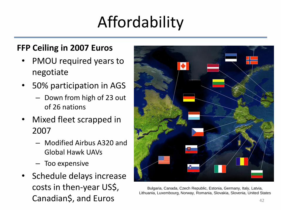
Affordability

FFP Ceiling in 2007 Euros

• PMOU required years to negotiate

• 50% participation in AGS– Down from high of 23 out

of 26 nations

• Mixed fleet scrapped in 2007– Modified Airbus A320 and

Global Hawk UAVs

– Too expensive

• Schedule delays increase costs in then-year US$, Canadian$, and Euros 42

Bulgaria, Canada, Czech Republic, Estonia, Germany, Italy, Latvia,

Lithuania, Luxembourg, Norway, Romania, Slovakia, Slovenia, United States

Software Development

Highest-Risk Element

• Growth in ESLOC– Requirements

• Configuration Management– Across many companies

• Different levels of CMMI certification

• Integration of Components– Software modules

– Hardware with software

– Other ISR assets and with intelligence gathering and analysis systems (e.g., MAGIC)

43

0

2

4

6

8

10

12

14

16

<0.25 0.50 0.75 1.00 1.25 1.50 1.75 2.00 2.25 2.50 2.75 3.00 3.25 3.50 3.75 4.00 > 4.00

Fre

qu

en

cy

ESLOC Count Growth Factor (Final/Estimate); Bin Endpoints

Growth in Count of ESLOC

Median CGF = 1.14

Mean CGF = 1.73CV = 95%

“The first 90% of the code accounts for the

first 90% of the development time. The

remaining 10% of the code accounts for

the other 90% of the development time.”

(Tom Cargill)

Software Development

Highest-Risk Element

• Demand for “Noble Work”– Software versus laying coaxial cable

• Knowledge gain

• Leverage for follow-on work

• NATO owns design but not code

• Schedule for MOB Development– Test facilities and equipment for

software

44

International Participation

45

Prime: Northrop Grumman Integrated Systems Sector International, Inc

Prime 2nd Level Subs Country

NGISSII

USA

Northrop Grumman Systems Corp (NGSC)

USA

CASSIDIAN (EADS) Germany

Selex Galileo Italy

General Dynamics Canada Canada

Kongsberg Norway

Potential subs to Cassidian: Retia ICZ (Czech

Republic); Aktors (Estonia); Dati (Latvia); Elsis

(Lithuania); Konstrukta (Slovakia); Hermes Soft

Lab (Slovenia)

3rd Level SubsNations

Bulgaria

Czech Republic

Denmark

Estonia

Latvia

Lithuania

Luxemburg

Romania

Slovakia

Slovenia

AGS CV and Scenarios

Choice of CV

• AGS a NATO rather than U.S. acquisition program. But,– Direct commercial sale to Northrop

Grumman

• Total System Performance Responsibility

– Based on U.S. Global Hawk

– Most of costs to be incurred in U.S.

• Many risk elements– Therefore, robust CV of 51% used

• Quantity-adjusted in then-year dollars (and Euros)

• Based on complete sample at MS B

Scenarios

• Baseline– Mostly likely

• Pessimistic– Unfavorable yet plausible

• Resource-Constrained– To meet ceiling price

46

Scenario Parameters

47

Elements Baseline Pessimistic ConstrainedExchange rate $1.35 per € $x.xx per € $x.xx per €

Inflation rate 3.00% x% x%

slip in schedule

Quantities/Schedule FY11 FY12 FY13 FY14 FY15 FY11 FY12 FY13 FY14 FY15 FY11 FY12 FY13 FY14 FY15

UAVs 2 2 2 2 0

Ground Stations change in quantities

Transportable 1 1 1 1 0 and schedule

Mobile 2 3 3 3 0

ESLOC Count No growth x% increase No growth

Radar 91% learning x% learning 91% learning

Int'l Participation Built-in redundancy x% delta to SE/PM Built-in redundancy

Affordability Unconstrained Unconstrained Constrained

S-Curve for NATO AGS

48

Cost values not displayed because of business sensitivity

0%

20%

40%

60%

80%

100%

€0.0 €0.5 €1.0 €1.5 €2.0 €2.5 €3.0

Esti

mat

ed

Cu

mul

ativ

e P

rob

abili

ty

Estimated Acquisition Cost in Billions of Then-Year Euros

Estimated Acquisition Cost of NATO AGS

Baseline Scenario● $1.35 per Euro● No growth in ESLOC; learning on MR-RTIP● Inflation at 3%; no delta for NATO work

Baseline CV of 51%with 95% Confidence Interval

Mean Median

Pessimistic Scenario● $x.xx per Euro● x% growth in ESLOC● x% learning on MP-RTIP● Cost delta for NATO work

• Inflation at x% per year23% probability of cost increase

S-Curve for NATO AGS

49

0%

20%

40%

60%

80%

100%

€0.0 €0.5 €1.0 €1.5 €2.0 €2.5 €3.0

Esti

mat

ed

Cu

mul

ativ

e P

rob

abili

ty

Estimated Acquisition Cost in Billions of Then-Year Euros

Estimated Acquisition Cost of NATO AGS

Baseline Scenario● $1.35 per Euro● No growth in ESLOC; learning on MR-RTIP● Inflation at 3%; no delta for NATO work

Baseline CV of 51%with 95% Confidence Interval

Mean Median

Pessimistic Scenario● $x.xx per Euro● x% growth in ESLOC● x% learning on MP-RTIP● Cost delta for NATO work

• Inflation at x% per year23% probability of cost increase

10% CV yields estimate at 99.9995Cum Percentile

Cost values not displayed because of business sensitivity

• Hypothetical Option– CV of 10%

– Pessimistic estimate

• Five in one million chance of costs reaching that level or higher!

– Deceives stakeholders

• Underestimates probability

• Take away– Essential to use

benchmark data

– Perform “deep dive”

S-Curve Tool

50

• Excel based– Reflects historical CVs and Cost

Growth Factors (CGFs)

– Supports both

• Monte Carlo simulation

• eSBM

• Allows practitioners to– Perform internal V&V

• Compare their estimated S-curves to curves using benchmark CVs and CGFs

– Perform assessments and reconciliations

• Compare ICE and Program Office S-curves

– Generate graphics

• eSBM POC– Dr. Paul Garvey, MITRE

• Tool POCs– Mr. Peter Braxton

– Mr. Richard Lee

• Tool and eSBM paper on NCCA’s website– At www.ncca.navy.mil

Backup

51

CVs: Calculation Issue

52

• “… a central issue of risk analysis:– We are trying to characterize within-program risk

• But “Cost is an unrepeatable experiment,” and we only ever get one observation for each historical program

– Thus, we are stuck using data from cross-programrisk

– We must cleverly devise a model that explains the former, while using historical data from the latter”

“The Perils of Portability: CGFs and CVs,”

Peter J. Braxton, Richard C. Lee, Kevin M. Cincotta,

Jack Smuck, Megan Guild, and Richard L. Coleman;

SCEA/ISPA Conference 2011

Translation of BY$ CGFs Into Costs

53

0

1

2

3

4

5

6

7

8

9

$0.2 $0.4 $0.6 $0.8 $1.0 $1.2 $1.4 $1.6 $1.8 $2.0 $2.2 $2.4 $2.6 $2.8Fr

eq

ue

ncy

CE Relative to a BE of $1.0 in Any Dollar Unit (e.g., Billions)

Acquisition Cost Outcomes from MS B for "All" DON MDAPs (Translation of CGFs into Normalized BY$; Unadjusted for Q∆s)

Mean = 1.0CE = BE

CE = $2.2B in FY10$ (BE = $1.0 )

CE = $1.0B in FY10$ (BE = $1.0 )

CE = $1.4B in FY10$ (BE = $1.0 )

Steps:– Inflate each ratio to common

year (e.g., FY2010)

– Normalize CGFs to mean of 1.0

• $CE = $BE at the mean

– Each $CE now interpretable as a cost outcome per dollar of $BE

• Same units of measurement

• Same year dollars

– CV is unchanged

• Computation also holds for BY$ quantity adjustments

Sequence of 50 BY$ CGFs: CE/BE1,1984, CE/BE2,1978, CE/BE3,1986, …, CE/BE50,2004

where i,j = observation number, base year of numerator and denominator

CV of costs & CGFs = 63%Desirable Statistical Properties:

CV independent of base year

CV independent of unit of measurement

Questionable Statistical Property:

CV invariant with respect to program size

Different raw indices for different SAR base years; purely conceptual since ratios won’t change

Pedagogical aid

Military Reading List

54

• With the Old Breed, E. B. Sledge– Wall Street Journal calls this book one of the “top five” ever in

describing any battle in the 20th century. A mortarman (MOS 0341) in the First Marine Division gives his account of fighting on the front lines in the Pacific campaigns of Peleliu and Okinawa.

• Unbroken, Laura Hillenbrand– The author of “Seabiscuit” chronicles the ordeals of Louis Zamperini,

an Olympic miler, who survived incredible hardship and torture when his B-24 Liberator crashed in the South Pacific in WW II.

• Ambush Alley, Tim Pritchard– According to many, “the most extraordinary battle of the Iraq war. “

• Inside Delta Force, Eric Haney– A gripping account of the formation, operation, and skills of America’s

elite counter-terrorism unit.

• Horse Soldiers, Doug Stanton– U.S. Special Forces defeat the Taliban in Afghanistan shortly after 9/11.

• Ender’s Game, Orson Scott Card

– Aliens have nearly destroyed the human race in two attacks. Our survival now rests entirely in the hands of a young genius, Ender Wiggin.

– Officially recommended as “professional reading” by the U.S. Marine Corps.

– I picked this one up at Quantico.

Nonfiction Fiction