Developing Thinking in Statistics (Published in association with The Open University)

StatisticsDEVELOPING THINKING IN

ALAN GRAHAM

Developing Thinking in Statistics

00_PRELIMS.QXD 16/1/06 12:56 pm Page i

00_PRELIMS.QXD 16/1/06 12:56 pm Page ii


Alan Graham

The Open University in association with Paul Chapman Publishing

00_PRELIMS.QXD 16/1/06 12:56 pm Page iii

© The Open University 2006

First published 2006

Apart from any fair dealing for the purposes of research or privatestudy, or criticism or review, as permitted under the Copyright,Designs and Patents Act, 1988, this publication may be reproduced,stored or transmitted in any form, or by any means, only with theprior permission in writing of the publishers, or in the case of reprographic reproduction, in accordance with the terms of licencesissued by the Copyright Licensing Agency. Enquiries concerningreproduction ouside those terms should be sent to the publishers.

Paul Chapman Publishing A SAGE Publications Company1 Oliver’s Yard55 City RoadLondon EC1Y 1SP

SAGE Publications Inc2455 Teller RoadThousand Oaks, California 91320

SAGE Publications India Pvt LtdB-42, Panchsheel EnclavePost Box 4109New Delhi 110 017

Library of Congress Control Number: 2005934566

A catalogue record for this book is available from the British Library

ISBN-10 1-4129-1166-4 ISBN-13 978-1-4129-1166-5ISBN-10 1-4129-1167-2 ISBN-13 978-1-4129-1167-2 (pbk)

Typeset by Pantek Arts Ltd, Maidstone, KentPrinted in Great Britain by the Cromwell Press,Trowbridge,Wiltshire Printed on paper from sustainable resources

00_PRELIMS.QXD 16/1/06 12:56 pm Page iv

Contents

Author viBook Series viiDeveloping Thinking in Statistics viiiAcknowledgements xi

Block 1 1

1 Describing with Words and Numbers 22 Comparing with Words and Numbers 183 Interrelating with Words and Numbers 344 Uncertainty 48

Block 2 61

5 Describing with Pictures 626 Comparing with Pictures 787 Interrelating with Pictures 938 Picturing Probability 110

Block 3 129

9 Describing with ICT 13010 Comparing with ICT 14511 Interrelating with ICT 16012 Probability with ICT 177

Block 4 193

13 Models and Modelling 19414 Statistical Investigation 20815 Teaching and Learning Statistics 219

Comments on Tasks 231References 266Index 269

00_PRELIMS.QXD 16/1/06 12:56 pm Page v

Author

Alan Graham has written over 20 short plays for BBC Schools Radio under the seriestitle Calculated Tales. Over the last 10 years, his work has concentrated on two mainareas, Statistics and Graphics calculators. He has published numerous books in theseand other areas, including Teach Yourself Statistics, Teach Yourself Basic Maths and theCalculator Maths series.Alan's main goal has been to help make the learning of mathe-matics both fun and accessible to all, taking in a variety of contexts including musicand art.

00_PRELIMS.QXD 16/1/06 12:56 pm Page vi

Book Series

This is one of a series of three books on developing mathematical thinking written bymembers of the influential Centre for Mathematics Education at The OpenUniversity in response to demand.The series is written for primary mathematics spe-cialists, secondary and FE mathematics teachers and their support staff and othersinterested in their own mathematical learning and that of others.

The three books address algebraic, geometric and statistical thinking. Each bookforms the core text to a corresponding 26-week, 30-point Open University course.

The titles (and authors) are:

Developing Thinking in Algebra, John Mason with Alan Graham and Sue Johnston-Wilder, 2005 Developing Thinking in Geometry, edited by Sue Johnston-Wilder and John Mason,2005 Developing Thinking in Statistics, Alan Graham, 2006

These books integrate mathematics and pedagogy. They are practical books towork through, full of tasks and pedagogic ideas, and also books to refer to when look-ing for something fresh to offer and engage learners. No teacher will want to bewithout these books, both for their own stimulation and that of their learners.

Anyone who wishes to develop an understanding and enthusiasm for mathematics,based upon firm research and effective practice, will enjoy this series and find it chal-lenging and inspiring, both personally and professionally.

00_PRELIMS.QXD 16/1/06 12:56 pm Page vii


Statistical thinking will one day be as necessary a qualification for efficient citizen-ship as the ability to read and write. (H.G.Wells, 1865, quoted in Weaver, 1952)

Statistics is a key area of the school mathematics curriculum where mathematics andthe real world meet.The term ‘data handling’ is sometimes used to refer to the samething as ‘statistics’. In this book, however,‘statistics’ is given a wider meaning than ‘datahandling’, covering the full range of ideas and concepts that inform one’s thinkingwhen posing and tackling real-world problems where data are used.

Although potentially a subject where teaching can be motivating and relevant toeveryday concerns, statistics is nevertheless sometimes seen as boring, predominantlyinvolving mechanical calculation.The aim in writing this book is to help teachers andothers interested in statistical thinking to become excited about and inspired by thebig ideas of statistics and, in turn, to teach them enthusiastically to learners.

INTRODUCTION

This book is for people with an interest in statistics/data handling, whether as alearner or a teacher, or perhaps as both. By working actively on the tasks rather thansolely reading the text, you will gain in a number of ways.

For example, you will:� be challenged to question your own understanding of statistical thinking;� come into contact with a number of pedagogic strategies and principles that teach-

ers will likely find useful in preparing for and conducting lessons;� engage with a number of theoretical ideas about teaching and learning;� learn more about working on and designing statistical tasks.

Throughout the book, tasks are offered for you to think about for yourself and, prob-ably after some modification, to use with learners. It is vital to work on themyourself, in order to have immediate experience of what the text is highlighting.Should they seem too simple, or occasionally out of reach, then you can adapt thetasks so that you feel personally challenged by them. Should you wish to try out simi-lar ideas with other learners, you will almost certainly need to adapt both thestructure and the presentation of tasks so as to render them appropriate to their needsand experience.

Mention was made above to ‘big ideas’ – these include:� measurement;� sampling;� modelling;� variation;

00_PRELIMS.QXD 16/1/06 12:56 pm Page viii

� drawing practical inferences;� randomness;� uncertainty.

Such topics are presented here by means of a variety of approaches, including infor-mation and communication technology (ICT) based simulations and the medium ofwhat is referred to as ‘telling’ stories and events. A ‘telling’ story is an important teach-ing strategy of the sort that has been used for several millennia (from biblical parablesand Aesop’s fables to problem pages found in modern magazines).

One of the problems with statistics is that it is a subject that comes with somethingof a reputation. Spend a few minutes now working at Task 0.1, which asks you toexplore different negative attitudes to statistics.You are encouraged to spend severalminutes thinking about this (and each subsequent) task and actually to write some-thing down.As you will find in the later chapters, many of the key ideas of the bookare presented in the context of such tasks.There is benefit to be gained from readingthe comments to be found either at the end of the book (they start on p. 231) or, onoccasion, as the text continues.The benefit will be considerably greater as a conse-quence of your having already worked and reflected on the questions posed and theissues raised. (Those tasks that have specific comments at the back of the book aremarked with a ‘C’ in the task header.)

Developing your ideas about what statistics is forms a large part of what this book isabout. So a good place to start is with your current sense of the meaning and set ofconnotations of this term.

There is obviously no ‘right’ answer to this question.You may have written somethingincluding ‘working with tables of data’ or ‘calculations with real-world numbers’.Alternatively, you may have written something about the big ideas in statistics, such as‘variability’ or ‘uncertainty’.

DEVELOPING THINKING IN STATISTICS ix

Task 0.1 Attitudes CRead the five statements below and try to express what attitudes may lie behind these observations.

(a) I’m a people person, not a numbers person.

(b) £1 000, £1 million, £1 billion, whatever. It doesn’t matter, as long as you do something aboutthe problem!

(c) I can’t even balance my cheque book!

(d) Will I need to know that for the exam?

(e) Lies, damned lies and statistics!

Task 0.2 What is ‘Statistics’?

What does the word ‘statistics’ mean to you? Write a sentence or two that captures your presentunderstanding.

00_PRELIMS.QXD 16/1/06 12:56 pm Page ix

As you will see in working through this book, emphasis is placed on the ‘big ideas’of statistics.These are the unifying concepts around which the day-to-day routinetasks of data handling gather (statistical calculation, drawing graphs, and so on), with-out access to which learners would be able to make little sense of the subject.

STRUCTURE OF THE BOOK

The book consists of 15 chapters.These are divided into four blocks, the first three ofwhich have four chapters each, whose contents run roughly parallel to one another,block by block.The first chapter of a block focuses on describing, the second on com-paring and the third with interrelating (in the sense of connecting two variables), whilethe fourth is concerned with various aspects of uncertainty (particularly probability).

The underlying theme of Block 1 is ‘words and numbers’. Block 2 focuses on pic-tures and graphs, while Block 3 is concerned with learning and teaching with ICT(specifically the graphics calculator, the spreadsheet and a computer statistical pack-age). In these first three blocks, each chapter has five sections, whose numberinglocates both the chapter and the section itself: Section 7.2 is the second section inChapter 7.These sections vary both in page length and in the time that you may wishor need to spend on them. However, there is an expectation that each section is basedon a notional average of two hours’ work.The fifth section of each chapter addressespedagogic issues concerned with the teaching and learning of statistics in school.

The final block has only three chapters in it, which first look at models and model-ling, then at statistical investigations before, finally, providing an overview of issuesrelating to teaching and learning statistics.

SUMMARY

To use this book effectively, you will need to engage with the tasks yourself, makeobservations about what you notice, both in your activity and in reflection upon yourown performance. Do not be distressed by getting stuck for a while on a task, as thisprovides an opportunity for you to experience the creative side of statistical thinkingand to learn something about pedagogy from the point of view of a learner. If a taskseems easy, then modify it so as to challenge yourself; if, after a reasonable period ofstruggle on your part, it seems too hard, find some way to simplify it. At the end ofeach chapter, you will be asked to reflect upon implications for teaching – in particu-lar, for promoting statistical thinking with learners. Should you have the opportunity,it is strongly recommended that you try out suitably modified tasks with learners, soyou can connect their experience with your own on similar tasks.

x DEVELOPING THINKING IN STATISTICS

Chapter: Describing

typical block

Chapter: Comparing

Chapter: Interrelating

Chapter: Uncertainty

Development

typical chapter

DevelopmentDevelopmentDevelopmentPedagogic issues

Tasks

typical section

CommentsText

00_PRELIMS.QXD 16/1/06 12:56 pm Page x

Acknowledgements

The writers and the publishers would like to thank the following for allowing theirwork to be reproduced in the book.

The Office for National Statistics for permission to use data from Social Trends 34(March 2005) in Figures 2.3 and Tables 5.1 and 5.2. Crown Copyright material isproduced under Class Licence Number C01W0000065 with the permission of theController of HMSO and the Queen’s Printer for Scotland.

The Daily Telegraph and Fischbacher, B (12th April 2005) for permission to repro-duce the photographs taken from the article by Fleming,‘Smiles that destroy the mythof female intuition’ in Chapter 2.

The American Statistician 35 (2) 1981, for permission to use Ehrenberg’s Tables fromthe article ‘The Problem of Numeracy’, in Tables 3.3 and 3.4.

The United Nations Millennium Indicators Database for permission to use the data inTable 3.5

The Gallup Organisation Inc., Princeton, NJ for permission to use data from‘Teens’ Supernatural Beliefs’ (1988) in Table 4.2.

Graphics Press USA, for permission to use John Snow’s map of the patterns ofcholera infection in Figure 5.3 and to reproduce the table in Table 6.1 from the VisualDisplay of Quantitative Information,Tufte E W (2001).

Michael Friendly, University of York, Canada (http://yorku.ca) for permission touse the diagram ‘Causes of Mortality in the Army in the East’ in Figure 5.9.

The New York Times Agency for permission to use the photograph in Figure 6.1.Lucent Technologies Inc./Bell Labs for permission to reprint the photograph of

John Tukey, Figure 6.4.Graphics Press, USA for permission to use the 1985 timetable of the Tokaido Line

at Yokohama Station, Sagami Tetsudo Complany, taken from Tufte, E W (1990) inFigure 6.8.

The Minerals Council of Australia for permission to use data from their informa-tion sheet ‘Olympic men’s 100m sprint results in athletics’ in Table 7.2.

NatureVol. 431, 30th September 2004, for permission to use the figure on the win-ning Olympic 100-metres sprint times for men and women in Figure 7.4.

The Daily Express (Express Newspapers), 14th June 2002, for the table of rainfallfigures for June in Stratford-Upon-Avon, taken annually over a ten year period inTable 7.3.

Nick Sinclair for the National Portrait Gallery for permission to use the photo-graph of Sir Richard Doll in Figure 7.8.

David Tideswell for permission to use the photograph of robins in Figure 8.6.The Guardian 4th December 2004 for permission to use the article by Hooper J

‘Curse of 53, Italy’s unlucky number’ in Figure 8.13.

00_PRELIMS.QXD 16/1/06 12:56 pm Page xi

00_PRELIMS.QXD 16/1/06 12:56 pm Page xii

Introduction to Block 1

Statistical ideas can be expressed using alternative andcomplementary forms: words and numbers, pictures and ICT.Block 1 of this book looks at statistical ideas from the point ofview of how they can be expressed using words and numbers,while pictures and ICT are the central themes of Blocks 2 and 3.

These first four chapters cover, in turn, the following ways ofthinking: describing, comparing, interrelating and dealing withuncertainty.A variety of statistical ‘big ideas’ are explored – forexample, relative and absolute differences, the notion ofvariability and the distinction between a statistical and a cause-and-effect relationship.

A number of useful and important teaching issues are offered;for example, the gambit of providing learners with ‘telling tales’that are designed to illustrate an important statistical idea in aninteresting and memorable context. Constructivism is an area ofeducational philosophy that describes how learners ‘construct’meaning in their learning and you are asked to consider howthis idea might relate to statistics learning.You will also beshown, and asked to use, a four-stage framework for tackling astatistical investigation.

01_CHAP 1.QXD 12/1/06 4:37 pm Page 1

1 Describing with Words and Numbers

In general, descriptions of things can be verbal or numerical in nature.This chapterexplores some similarities and differences between these two forms of describing.

Some people have a good eye for shape and can do these sorts of tasks fairly easily.Others find it difficult to remember the details and perhaps tend to get mixed up, forexample, when trying to remember shapes of similar type such as the last two. Oneproblem is that there seems to be nothing that enables you to see these shapes as awhole – they appear to be just five unconnected things.

So, these five shapes are not unconnected after all. It is the experience of most peoplethat, having grasped the ‘bigger picture’, the component parts are subsequently easierto discern. It is a facet of human nature that different people attend to different thingsand, indeed, the same person attends to different things at different times.This phe-

Task 1.0.1 Shapes

Spend about 20 seconds looking at the five shapes below. Then close the book and try to draw them asaccurately as you can.

Task 1.0.2 The Bigger Picture

Place two straight edges horizontally across the top and bottom of the drawings above. Now look not atthe shapes themselves but at the spaces in-between. Does a word jump out at you? Keep looking untilit does. Eventually, you should find that that the individual shapes seem to have a ‘life’ of their own.Now have another go at drawing the five shapes. Is the task suddenly easier?

01_CHAP 1.QXD 12/1/06 4:37 pm Page 2

nomenon is sometimes referred to as ‘stressing and ignoring’, a phrase that will beused more than once in this book. It describes an important aspect of learning,whereby, in order for a learner’s attention to be directed to one aspect of a problem, itis helpful to shut out its other features.

It seems that information is hard to absorb when each fact stands in isolation fromothers, unconnected to a wider context or some overarching ‘big idea’. Knowingabout these big ideas will help provide learners with coherence and meaning to themany facts and techniques they are expected to acquire from a statistics course. Anawareness of the big ideas enables a newly learned technique to be applied to othersituations in the future, not just the one in hand.As novelist George Eliot observed:

It has been well said that the highest aim in education is analogous to the highestaim in mathematics, namely, not to obtain results but powers, not particular solu-tions, but the means by which endless solutions may be wrought.

(Quoted in Carlyle, 1855; italics in original)

In common with many other disciplines, one big idea stands out from all others andthat is describing. As you can see from the main title of this chapter, this is its centraltheme. Section 1.1 suggests that, in statistics, the central building block of thinkingstatistically is data. As Sherlock Holmes once remarked to Dr Watson, ‘You weretrying before you had sufficient data, my friend; one can’t make bricks without straw’(quoted in Hanson, 2001, p. 628).

The two main themes in the first section are sampling and designing a question-naire. Section 1.2 then explores questions of measurement, and you will beintroduced to a number of different types of measuring scales. Data can involve bothvery large and very small numbers and how these are handled and represented isexplored in Section 1.3. Summarising data often takes the form of calculating aver-ages and spreads: these ideas are considered in Section 1.4.The final section looks atteaching and learning issues.

1.1 DESCRIBING WITH DATA

Depending on each individual’s personality and training, everyone sees the world in aslightly different way. An artist’s ways of seeing are predominantly tactile and visual,exploiting colour, texture and shape. A historian draws on and produces descriptions

DESCRIBING WITH WORDS AND NUMBERS 3

Task 1.0.3 The Big Ideas of Statistics CSpend a few minutes looking at Table 1.1, which lists some of the know-how and techniques of statis-tics (row 1) and some big ideas (row 2). To help you to get a better feeling for the nature of a big idea,try to match up each item in row 1 with one or more corresponding terms in row 2. Are there any termshere you are unfamiliar with? How might you find out what they refer to?

TABLE 1.1 Matching Up

Know-how and techniques Understanding and knowing how to calculate or draw:the range, the median, a bar chart, a scatter plot, the quartiles

Big ideas Summarising, measures of location, spread and variation, interrelating

When you see a ‘C’ in the task header, remember to check ‘Comments on Tasks’ at the end of the book.

01_CHAP 1.QXD 12/1/06 4:37 pm Page 3

and analyses of past events, in order to gain insights about human behaviour. Anauthor will describe her or his world with words, using metaphor, onomatopoeia and,on occasion, poetry. Each of these ways of seeing is valuable, and, when takentogether, provide rich, diverse and complementary perspectives on human concerns.

What, then, is the particular statistical view of the world? It is essentially one basedon quantitative descriptions, where the world is viewed on the basis of measures andcounts, otherwise known as statistical information or data. Outside a narrow educa-tional context, data are rarely collected without a clear reason or purpose.Typicalquestions that may inspire the need for data collection may be of the form,‘How bigis A?’ or ‘Is A bigger than B (and by how much)?’ or ‘How is X related to Y?’.Thenature of these questions is considered in more detail in, respectively, the first, secondand third chapters of each of the first three blocks.

Once data have been collected, they need to be analysed in order for interesting orunexpected patterns to be identified.These patterns must then be interpreted in thecontext of the original question that started the investigation.

Four stages have now been identified that correspond to the following four impor-tant phases of a statistician’s work. In summary, these are:

P stage: pose a question;C stage: collect relevant data;A stage: analyse the data;I stage: interpret the results in the context of the question.

These four stages are referred to as the PCAI framework for conducting a statisticalinvestigation: they are considered more fully later in the book, particularly inChapters 2 and 14.

In this section, you will focus on the C stage of data collection, looking at twoimportant aspects of how data are collected.The first concerns exploring how andwhy samples are taken in statistical work. In the second, you will look at how socialdata are collected, raising issues of polling and questionnaire design.

Sampling

A census refers to data collection where all the people or items of interest are meas-ured or surveyed. However, when collecting information about a large population, itis often too inconvenient or expensive to measure every item: you must make dowith taking a representative sample.This might take the form of choosing items ran-domly from a production line and measuring them to ensure that the values fallwithin acceptable tolerance limits.Alternatively, you may wish to survey the opinionsof customers on how satisfied they are with the layout of a store or invite people toreveal their voting intentions just before a general election.

4 BLOCK 1

Task 1.1.1 Thinking it Through CImagine that you wish your learners to carry out a poll of television viewing habits of young people. Thiswill involve taking a sample from the learners at their school. Before carrying out the poll, there are cer-tain questions that they will need to think through about choosing their sample. Write down two orthree of these questions. How might you help learners to tackle these questions sensibly?

01_CHAP 1.QXD 12/1/06 4:37 pm Page 4

Inevitably, in any discussion with learners about choosing a sample, a key point toemerge will be the importance of choosing a representative sample. (Sampling is lookedat again in Section 14.2.)

Questionnaire Design

Although many scientific and industrial data are collected by direct measurement,‘social’ data (for example, people’s opinions on social issues like crime and health)usually require the use of a well-designed questionnaire. Unfortunately, the wordingof questions in newspaper questionnaires is sometimes blatantly loaded or biased.Look at this one published several years ago in the Daily Star under the headline‘We’ve had ENOUGH!’

1. I believe that capital punishment should be brought back for the followingcategories of murder:Children [ ] Police [ ] Terrorism [ ] All murders [ ].2. Life sentences for serious crimes like murder and rape should carry a mini-mum term of:20 years [ ] 25 years [ ].3.The prosecution should have the right of appeal against sentences they con-sider to be too lenient [ ].Tick the boxes of those statements you agree with and post the coupon to:VIOLENT BRITAIN, Daily Star, 33 St. Bride St., London EC4A 4AY.

The fact that this article appeared alongside articles with headlines such as ‘Mymother’s killer runs free’ and ‘Hang the gunmen’ is likely to have biased the responseto these questions. But it is the nature and limited range of choices offered that dis-torts the survey even more. For example, there are no tick boxes available for peoplewho do not support the death penalty or who favour alternative forms of punishmentto imposing longer jail sentences.

It may not be too surprising to learn that, of the 40 000 readers who responded(and just how representative were they of the readers of the Daily Star or the popula-tion as a whole?), 86% favoured restoring the death penalty for murder, 92% wanted a25-year minimum sentence for serious crimes of violence and 96% supported theprosecution right of appeal against ‘too lenient’ sentences.

In this Daily Star example, the bias was obvious. However, bias can occur, even in awell-designed questionnaire where there is no intention to deceive.As Steven Barnett(former chairman of the Social Research Association) argued in an article in theGuardian newspaper in 1989:

Ultimately, however reliable the sample, social surveys consist of an aggregationof very short dialogues between two complete strangers.When these dialoguesattempt to address intimate questions of feelings and opinions on social issues,the scope for misinterpretation is considerable. (p. 5)

As can be seen from the Daily Star questionnaire, how the question is worded canhave a crucial impact on the response given. (For example, many people are stronglyin favour of the democratic right to withhold their labour in an industrial dispute, butwould personally draw the line at striking.)


01_CHAP 1.QXD 12/1/06 4:37 pm Page 5

Some people think this sort of research is invalid on the grounds that, ‘they didn’t askmy opinion’. This is an unfair criticism – provided the sample has been sensiblychosen to represent, fairly, the overall population, its findings should provide a usefulsnapshot of opinion. Second, they may feel it to be deceitful, because sometimes sur-veys are used as a cheap device for pitching a sale about a related product.This is avalid point and a good reason for avoiding co-operation with certain ‘surveys’ con-ducted in the street or on the phone. Finally, people may think that surveys are awaste of time because the questionnaires they see are designed by school pupils carry-ing out a shopping survey or those in newspapers like the Daily Star example.Thisproblem is compounded by the fact that many newspaper polls (for example, thosesoliciting voting intentions before an election) are carried out in a matter of days,with little time to check wordings or test accuracy.

Nevertheless, despite these obvious dangers and drawbacks, social research can fulfilan important and valuable function in identifying areas of need in society and tryingto ensure that resources are used sensibly.This sort of justification for social research israrely explained to the general public and is certainly an aspect of statistics that shouldbe discussed with learners.As Steven Barnett (1989) remarked:

Whatever the hazards, however, survey research has a critical role in the devel-opment of much social policy. Patterns of employment, of health care, oftransport, or of criminal activity pose awkward social questions requiring urgentsolutions which compete for scarce resources. Results of large-scale socialresearch can therefore provide the basis for decisions which affect people’s lives.For this reason, the responsible social scientist will take every conceivable meas-ure to ensure that the scope for misunderstandings are reduced to an absoluteminimum. (p. 5)

1.2 DESCRIBING BY MEASUREMENT

The philosopher Aristotle (384–322 BCE) described a human being as ‘a rationalanimal’, believing in the power of reason as a natural human state.This view largelydisappeared in the ‘dark ages’ (roughly 400–1300) in favour of the view that peopleshould act on the basis of faith and emotion. René Descartes (1596–1650) was a keysupporter of the re-emergence of rationality and argued that people should actaccording to the evidence of their senses and be informed by the power of reasoningrather than making decisions on the basis of divine inspiration.

However, rational decision-making is still treated with suspicion in certain quarters– based on a fear, perhaps, that individualism is being suppressed by the imposition of

6 BLOCK 1

Task 1.1.2 Your Opinion about Seekers of Opinion

What are your attitudes to social research? Do you feel it provides worthwhile data or is largely a wasteof time? If you do have negative feelings, try to note down precisely why you hold this view.

Task 1.1.3 Eliminating Questionnaire Bias CHow do you think reputable polling agencies like MORI and Gallup try to ensure that the questions theyask are as clear and free from bias as possible?

01_CHAP 1.QXD 12/1/06 4:37 pm Page 6

conformity, with no room to express one’s individual personality.This is an attitude ofmind raised in some of the quotations listed in Task 0.1. People are correct to besceptical when attempts to achieve rationality are conducted in a crass or inappropri-ate manner. People fear that decisions based on quantification and measurement maymiss the point – perhaps this runs the risk of including only the easy-to-identify fac-tors and under-representing more subtle human characteristics. As Frenchphilosopher and mathematician Blaise Pascal (1623–62) expressed it:

The heart has its reasons, which reason does not know. (1670, IV: 277)

Perhaps the moral here is that there are many ways of seeing the world, of which auseful and sometimes illuminating means involves quantification and statistical analysis.

Measuring Scales

The purpose of measuring is to describe things and the two most basic forms ofdescription are words and numbers. In the next task, you are asked to think aboutthese two ways of describing.

When different but related words are used as descriptors, it is often helpful to beaware how they relate to each other. Sometimes it is possible to elicit a natural order-ing for these words that may not have been obvious initially.

Task 1.2.2 shows that, depending on context, certain sets of words do sometimes have anatural order. Clearly, there are other sets of words that always possess a natural order-ing (for example, small/medium/large, months of the year, days of the week, and soon). However, care must be taken when the words are used in a cyclic arrangement –to take the example of days of the week, does Monday come before or afterThursday? The answer is that it depends which Monday and which Thursday you arereferring to.

Turn your attention now to numbers and their properties for describing things. Asyou will see from the next task, numbers also operate in different ways, depending oncontext.


Task 1.2.1 Words or Numbers CWhat are some strengths and weaknesses of using ‘words’ and ‘numbers’ to describe things? List someexamples of things that are better described by words and others that are better described by numbers.

Task 1.2.2 Only Words? CLook at the three lists of words below. Can you think of any sensible way of ordering them?

(a) sit, walk, roll, crawl, run;

(b) gold, wood, silver, ruby, paper;

(c) rayon, cotton, linen, silk, wool.

01_CHAP 1.QXD 12/1/06 4:37 pm Page 7

The next two sub-sections look at two key ideas in the area of measurement – theStevens taxonomy for sorting out measures and their properties, and the distinctionbetween discrete and continuous scales of measure.

The Stevens Taxonomy

There has long been confusion and debate about measurement and the nature ofmeasurement scales.This became a major issue in the field of psychophysics in the1930s. (Psychophysics is concerned with describing how anorganism uses its sensory systems to detect events in its envi-ronment.) In 1932, a British committee investigatedquestions such as: ‘By how much must the frequency of asound be raised or lowered before a person can just detecta difference in pitch?’ (Such a difference is referred to as alimen.) The committee concluded that subjective judgementsof this sort could not be a basis of measurement.

This is where Stanley Smith Stevens, a professor of psy-chophysics at Harvard University, joined the debate. Heargued that the fault lay not with the particular measures,such as the limen, but with the fact that there existed noclear schema for understanding the nature of measurement.In a seminal paper (Stevens, 1946), he described a taxonomyof measurement based on four classes of scales. He named these ‘nominal’, ‘ordinal’,‘interval’ and ‘ratio’ scales and they are discussed below.

A nominal (or naming) scale of measurement is used for named categories such asrace, national origin, gender, surname, and so on. For the purposes of counting suchdata, it is common to code the names with numbers: for example, 0 = male and 1 =female. Sometimes numbered data are actually nominal, in the sense that the numberis no more than a label, with no conventional quantitative significance: for example,the numbers on the shirts of footballers or marathon runners, telephone numbers anduniversity learner numbers are all nominal.All that can be done with nominal meas-ures is to count how many fall into each category (and maybe compute thecorresponding percentages).

An ordinal (or ordered) scale of measurement involves data which can be ranked inorder (first, second, third, and so on), but for which the numbers cannot be used forfurther calculation. For example, a questionnaire on attitudes to university fees may

8 BLOCK 1

Task 1.2.3 Twice CRead the statements below. If you feel that any are incorrect, write down why.

(a) Manchester United scored six – twice as many as their rivals Charlton Athletic.

(b) She turned up at 6 p.m. – twice as late as the advertised starting time of 3 p.m.

(c) He turned up six hours late – twice as late as his sister who came only three hours after theadvertised starting time.

(d) The temperature was 15 ºC, but the next day it was twice as hot, at 30 ºC.

(e) The first tremor measured 2.0 on the Richter scale. That was followed by one twice as strong –it measured just over 4 on the Richter scale.

S.S. Stevens(1906–73)

01_CHAP 1.QXD 12/1/06 4:37 pm Page 8

ask respondents to indicate their attitude on a five-point scale, ranging from 1 = verystrongly opposed to 5 = very strongly in favour.As with nominal data, the number ofresponses falling into each category can be counted and percentages calculated, butnow the values can be ordered by size. (Ideas of ordering were raised in Task 1.2.2.)

An interval scale of measurement is a rather subtle concept – numbers are used formeasurement of the amount of something, but the scale is such that the zero is arbi-trary. This idea occurred in Task 1.2.3, with the questions about time of day andtemperature. Zero degrees (0 °C) does not mean ‘no temperature’. It is an arbitrarypoint on the temperature scale associated with the temperature at which water freezesat sea level (under normal atmospheric pressure). Contrast this with measures such asmass or length: a length of 0 cm does mean ‘no length’ and something that is 20 cm istwice as long as something that is 10 cm. Most psychological tests, such as measures ofpersonality and academic ‘ability’, are interval measures. (If a learner receives zero onan exam, it does not mean that he or she knows nothing about the course.)

Interval data have all the properties of nominal and ordinal data but, additionally,the intervals between adjacent values are equal.This means that they can be addedand subtracted (so, 40 °C is 10 °C warmer than 30 °C or a person may increase theirIQ score by 5 points). However, the operations of multiplication and division do notapply appropriately to interval scales. For example, as you saw in Task 1.2.3, a temper-ature of 30 °C is not twice as warm as a temperature of 15 °C.

A ratio scale of measurement has all the properties of an interval scale but, addition-ally, the operations of multiplication and division can be used meaningfully.Thus, it isfair to say that an age of 16 years is twice as much as an age of 8 years, or that some-one weighing 66 kg is twice as heavy as someone weighing 33 kg. Change the yearsto days or the kilos to pounds and the relationship of ‘twice as much’ is unaffected.Examples of ratio measurements include mass, length, speed or acceleration and,unlike with interval scales, zero really does mean ‘none’ of whatever quantity is beingmeasured.

You can consolidate your understanding of Stevens’s taxonomy of measuring scalesby tackling Task 1.2.4.


Task 1.2.4 Testing Your Take on the Taxonomy C(a) Classify the following measures according to Stevens’s taxonomy:

(i) A questionnaire asking: ‘How would you rate the service of our catering staff?’

Excellent ( ) Good ( ) Fair ( ) Poor ( )

(ii) Windspeed, measured in knots.

(iii) Bathroom scales, measuring in kg.

(iv) The UK is made up of four separate countries: England, Scotland, Wales and Northern Ireland.

(v) Wind force, measured on the Beaufort scale (0 = calm, 1 = light air, 2 = light breeze, …,12 = hurricane).

(b) Is it possible for temperature to be measured on a ratio scale?

(c) How can time of day and time elapsed be distinguished using the Stevens taxonomy?

01_CHAP 1.QXD 12/1/06 4:37 pm Page 9

The Discrete/Continuous Distinction

There is another means of distinguishing types of measurement scale, namely, the dif-ference between discrete and continuous scales.

The distinctions in parts (a) and (b) above are essentially the same.Words like ‘howmany’ and ‘fewer’ refer to measures of discrete, separate, countable items, whereas ‘howmuch’ and ‘less’ refer to something that cannot be counted out, such as amount ofwater, size of slice of a pie, and so on.The terms used in statistics to make this distinc-tion are ‘discrete’ and ‘continuous’, respectively.

The key feature of a continuous variable is that, as the name implies, one valueflows continuously into the next with no gaps or steps. Between any two values of acontinuous variable there is an infinite number of other possible values. Examples ofcontinuous variables include height of plants in a nursery, air temperature and waitingtime in a dental surgery.

Contrast this with a discrete variable, where the possible values that it can take arerestricted, with gaps between adjacent values. Examples include size of household,marks scored in a test and outcome when rolling a die. It is not possible to have ahousehold size or die score of, say, 3.17. (It is, of course, possible to have an averagehousehold size of 2.4 or an average die score of 3.17, but these numbers arise as aresult of calculating an average and such averages are not usually an actual item of thedata from which they were calculated.)

10 BLOCK 1

Task 1.2.5 Grammar, Timothy! C(a) Overheard: Timothy, aged 9, was in a bookshop with his mum. Holding up the new Harry Potter

book, he said, ‘Mum, guess how much pages are in this book’.

Why is Timothy’s grammar incorrect?

(b) Distinguish the meanings of the words ‘fewer’ and ‘less’.

(c) What ‘big idea’ connects your answers to parts (a) and (b) and how does it relate to statistics?

Task 1.2.6 Distinguishing Discrete and Continuous Measures CLook at the measures below and classify them into ‘discrete’ or ‘continuous’ measurements.

(a) A child’s foot length.

(b) A child’s shoe size.

(c) The duration of a film.

(d) The time taken to run a race.

(e) The number of runners in a race.

(f) Air temperature.

(g) The number of matches in a box.

(h) The speed of a car.

(i) The number of goals scored in a season.

(j) Time displayed on a dial watch.

(k) Time displayed on a digital watch.

(l) Annual salaries of teachers.

01_CHAP 1.QXD 12/1/06 4:37 pm Page 10

Now look at the two sentences below and then tackle Task 1.2.7.

The UK is made up of fourseparate countries: England,Scotland,Wales and NorthernIreland.The UK is made up of four separate countries:Wales, England,Scotland and Northern Ireland.

One difficulty with making the discrete/continuous distinction is that, in the real world,measurement of a continuous variable can never be carried out with perfect accuracy.Inevitably, rounding reduces the number of possible values that the variable can takefrom a theoretical infinity of possibilities to something finite.This means that, in practice,all measurement can be thought of as being discrete. However, the distinction is still auseful one to make, particularly when it comes to displaying data graphically.

1.3 LARGE AND SMALL NUMBERS

There is no doubt that most measurement involves numbers; sometimes these can behuge numbers and at other times extremely tiny. It is often hard to know how toreact to being told certain numerical information without knowing whether it is a lotor a little.A ‘mental muscle’ that needs regular exercise is the ability to make sensible,‘ball-park’ estimates, particularly with large and small numbers. Estimation tasks are auseful and entertaining way of developing your number feel – finding out how bigthings are to some order of magnitude.

Rough Calculations

Some facts you either tend to know or not, as the case may be. (How far is it fromJohn o’Groats to Land’s End or what is the approximate population of the world?)Other ‘facts’ may not be known precisely, but with a bit of intelligent guesswork and afew ‘back-of-an-envelope’ calculations, a rough estimate can be made. Sometimes, forcertain purposes, a rough estimate is all that is required. For example, in 2004, a vandriver drove through Dover with 1 million cigarettes in the back.When questioned,he claimed these were for his ‘personal use’. On the basis of a rough calculation,Customs officials estimated that even a heavy smoker would have enough smokingmaterial for ‘personal use’ to last for 50 years!


Task 1.2.7 Wales Has Been Moved! CThe two sentences are identical except that, in the second, the word ‘Wales’ has been moved to a dif-ferent position in the sentence. Clearly, these sentences have exactly the same number of characters,yet they do not occupy the same number of lines of text – a matter of great importance to, say, a news-paper editor.

Try to explain this phenomenon, using the ideas of this section.

01_CHAP 1.QXD 12/1/06 4:37 pm Page 11

Having an understanding of the orders of magnitude of numbers is an important lifeskill that is best developed by letting learners explore a wide range of real-world con-texts, which is something for which statistics lessons provide many opportunities. Inthe next task, you are asked to think further about how this skill can be developed.

If you used a calculator with Tasks 1.3.1 and 1.3.2, you will, no doubt, have come intocontact with numbers expressed in scientific notation (also sometimes referred to as‘standard form’).This notation is inescapable when calculators and spreadsheets areused and is a topic that learners from age 14 on need to be able to handle with confi-dence. It is considered further in Task 1.3.4.

Visualising

In 1999, the eyes of the sporting world were focused on Wales with the opening ofthe Millennium Stadium, which was built on the historic Cardiff Arms Park site.Designed for all-year, all-weather use, the stadium was the first in the UK with aretractable roof and the first of its type in the world with 75 000 seats. If you havenever attended a major public event, it is hard to imagine what 75 000 people gath-ered together in one place looks like, let alone what it sounds like when they all startshouting or singing at the same time.What would help you or a learner to get a feelfor a number as large as this?

Writer Bill Bryson (2004) has a knack of making statistical information bothmeaningful and palatable to his readers, by providing a helpful mental picture of themagnitudes involved. Here are a few examples taken from his book, A Short History ofNearly Everything.

12 BLOCK 1

Task 1.3.1 Rough Estimates CMake a rough guess and then an estimate of the following. As you do so, think about the estimates andcalculations that you carried out along the way and what ‘facts’ and assumptions they were based on.

(a) How long will it take for 1 million seconds to tick by? (Make a guess before getting out your enve-lope.)

(b) How long would it take for 1 billion seconds to tick by? Note that modern usage of the word ‘billion’refers to 1000 million. (Make a guess before making your estimate.)

(c) The population of the world is roughly 6.5 billion people. How many people in the world die eachday?

(d) The population of the UK is roughly 57 million. How many cigarettes are smoked annually in theUK?

(e) How fast does human hair grow, in km per hour?

Task 1.3.2 Adapting Tasks CTake one of the five statements listed in Task 1.3.1 and adapt or extend it for use with another learner.

01_CHAP 1.QXD 12/1/06 4:37 pm Page 12

� A typical atom has a diameter of 0.00000008 cm. … Half a million of them linedup shoulder to shoulder could hide behind a human hair. (p. 176)

� An atom is to a millimetre as the thickness of a sheet of paper is to the height ofthe Empire State Building. (p. 177)

� Avogadro’s number, the number of molecules found in 2.016 grams of hydrogengas (or an equal volume of any other gas at the same temperature and pressure), isequal to 6.0221367 × 10^23, which is equivalent to the number of popcorn ker-nels needed to cover the US to a depth of 9 miles, or cupfuls of water in thePacific Ocean, or soft-drinks cans that would, evenly stacked, cover the Earth to adepth of two hundred miles. (p. 139)

� Astronomers today believe that there are perhaps 140 billion galaxies in the visibleuniverse. … If galaxies were frozen peas, it would be enough to fill a large audito-rium – … say … the Royal Albert Hall. (p. 169)

� The most striking thing about our atmosphere is that there isn’t very much of it. Itextends upwards for about 190 kilometres … if you shrank the Earth to the size ofa standard desktop globe, it would only be about the thickness of a couple of coatsof varnish. (p. 313)

� [On how far back the Cambrian era is.] If you could fly backwards into the past ata rate of one year per second, it would take you about half an hour to reach thetime of Christ, and a little over three weeks to get back to the beginnings ofhuman life. But it would take you twenty years to reach the dawn of the Cambrianperiod. (p. 395)

Here are some of the examples given in this section of very large and very smallnumbers.

� The number of seconds that have elapsed since the creation of the earth is about15000000000000000000.

� There are perhaps 140 billion galaxies in the visible universe.� Human hair grows at roughly 0.000000014 km per hour.� A typical atom has a diameter of 0.00000008 cm.

These are very extreme numbers and it is almost impossible to understand how largeor how small they are.The problem lies with the sea of zeros that such numbers con-tain when expressed in conventional notation. Scientific notation (sometimes calledstandard form) provides an alternative way of representing numbers that overcomesthis problem.


Task 1.3.3 Visualising Facts CHere are some facts. How would you try to visualise these numbers?

The capacity of the Millennium stadium, Cardiff: 75000 people.

The capacity of the Centre Court at Wimbledon: 15000 people.

The capacity of the London Palladium theatre: about 2200 people.

The length of time humans have been around (4 million years), compared with the length of time theearth has been around (4.6 billion years).

01_CHAP 1.QXD 12/1/06 4:37 pm Page 13

The number 37 200 can be written in standard form as 3.72 × 104 or sometimes as3.72E4.The number 0.00000437 can be written in standard form as 4.37 × 10–6 or some-times as 4.37E–6.

Handling numbers in standard form needs a fair degree of practice, as you will seefrom Task 1.3.5.

1.4 SUMMARISING – AVERAGES AND SPREADS

So far in this chapter, descriptions have come in the form of individual words or num-bers.An important feature of statistics is that, usually, many measures are made in order todescribe things.This may take the form of an experiment or a survey in which a batch ofdata items together represents the description in question. (A batch is another name for adata set.) This move from single numbers to many numbers is a very big idea in statistics,one that is not always obvious to learners when they first study the subject.

Once data have been collected, whether from a survey or scientific experiment orsomething else, it is often hard to ‘see the wood for the trees’. Some sort of organisa-tion or simplification is necessary in order to gain a sense of what the data seem to be‘saying’.Where possible, data can usefully be organised into a table (table layout is dis-cussed in Section 3.2) or summarised into a single figure (sometimes called ‘a statistic’).

If that single figure is a summary of where the data are centred (often called a measureof location), then the numerical summary is known as an average. If the aim of the sum-mary is to understand how widely dispersed the data are, then a measure of spread isneeded.Whatever the purpose of the summary (to describe the location or the disper-sion of the data), they have one thing in common – summarising enables a largenumber of figures to be reduced to a single representative figure.This has obvious bene-fits in terms of providing a useful overview. However, summaries inevitably bring

14 BLOCK 1

Task 1.3.4 Converting Numbers into Standard Form C(a) Using the two examples above as a guide, convert the following numbers into standard form.

15 000 000 000 000 000 000

140 billion

0.000000014

0.00000008

(b) Type these four numbers into a scientific or graphics calculator and press ‘=’ (or ENTER) to checkthat your answers to part (a) are correct.

(c) What are the advantages of displaying these numbers in scientific notation?

Task 1.3.5 Calculating with Standard Form CPredict what answer would be displayed on a calculator or spreadsheet to the following calculation:2.4E36 – 2.4E12. Then perform the calculation and explain why this answer has resulted. What issuesare there here that you might wish to share with learners?

01_CHAP 1.QXD 12/1/06 4:37 pm Page 14

corresponding costs in terms of the loss of data and an investigator needs to steer a sen-sible path between these two aspects, namely, too much and not enough information.

The three best-known measures of location are the three averages, the mean, themode and the median.

At a more advanced level, two other useful ‘averages’ in some circumstances are thegeometric mean and the harmonic mean.

The geometric mean: just as the arithmetic mean of two numbers is found by addingthem and dividing by two, the geometric mean is found by multiplying themtogether and then taking the square root.The geometric mean of n numbers is foundby multiplying them all together and then taking the nth root. (Finally, note that thegeometric mean cannot be used when any of the values are ≤0.)

An example of where the geometric mean is useful is in calculations of vibrating fre-quencies in the tuning of musical instruments.The vibrating frequency of middle C on apiano is 256 Hz.The vibrating frequency of the C above middle C (one octave above) istwice this value, at 512 Hz.There are 12 semitone intervals between these two notes andin order to ensure that the intervals are equal, the geometric mean must be calculated.One way of explaining this is that, as the 12 semitone steps of the octave together multi-ply to 2 (in order to double the frequency from 256 to 512), each step is the twelfth rootof 2, or roughly 1.059. So the semitone above middle C (named C sharp, written C#) hasa vibrating frequency of 256 × 1.059, or roughly 271 Hz; the next semitone in thesequence (named D) has a vibrating frequency of 256 × (1.059)2, or roughly 287 Hz; andso on all the way up to C above middle C, with a frequency of 512 Hz.

The harmonic mean: a common problem for learners is in the calculation of averagespeeds. If the average speed for the outward journey is, say, 40 kph and the averagespeed of the return journey is 60 kph, it is not the case that the average speed of theround trip is 50 kph.The arithmetic mean simply does not apply to this situation andwhat is required is the harmonic mean.This involves taking the following steps:

� take the reciprocals of the values 40 and 60: 1/40 and 1/60;� find the arithmetic mean of the reciprocals: (1/40 + 1/60)/2 = 5/240;� take the reciprocal of the result: the reciprocal of 5/240 = 240/5 = 48.

So, the overall average speed of the round trip is 48 kph.So, why does it work? In this particular example, further investigation by learners

may reveal that the key to understanding calculations involving speeds is to concen-trate on the time elapsed for each part of the journey. Since speed is equal to distancedivided by time, there is an inverse relationship between speed and time. It followsthat in order to average the times of the two parts of the journey, you need to find theaverage of the reciprocals of the two speeds.


Task 1.4.1 Learner Definitions CHere are plausible definitions of these three averages provided by a learner. Try to decide which iswhich and then, if required, improve the learner’s definitions.

Definition 1: If there are 20 values, it’s 10.

Definition 2: Add them together and divide by how many there are.

Definition 3: It’s the biggest frequency.

01_CHAP 1.QXD 12/1/06 4:37 pm Page 15

A message here for learners is that it is always useful to consider problems frombasic principles rather than mindlessly applying a formula.

In Section 1.2, you read about the Stevens taxonomy for classifying scales of measure-ment.This way of thinking is very helpful when checking which numerical summariescan and cannot be applied to certain measures. For example, since calculation of themean involves adding numbers together, this choice of summary would not be suitablefor nominal or ordinal data, where there is no uniform interval between values.This iseasiest understood with specific examples, as the next task will reveal.

1.5 PEDAGOGY: PREPARING TO TEACH A TOPIC

This section highlights some thoughts about teaching and learning statistics in rela-tion to the topics of this chapter.

There is clearly no single correct answer to these questions of preparation of a topic –people prepare in various ways, depending on their own subject knowledge, particularinterests and their perceptions of the needs of the learner(s) that they have in mind.

In this chapter, and indeed in all the chapters of the book as far as Chapter 12, the finalsection looks at pedagogic (that is, teaching) issues in terms of the following six themes.They will be referred to as the ‘Preparing to Teach’ framework (or PTT for short).

� Language patterns – learners may be using some of the technical terms and expres-sions already but perhaps without the standard mathematical meaning.

16 BLOCK 1

Task 1.4.2 Create Your Own Task CNow create a task of your own for helping learners to think about a measure of spread – the range.What might another measure of spread be?

Task 1.4.3 When Averaging is Appropriate CNote down four data sets, one each based on nominal, ordinal, interval and ratio measuring scales,respectively. Decide whether each can be summarised using the mean, the mode and the median. Tryto make a general conclusion (in the form of a table) about which forms of average operate correctlywith each of the four Stevens scales of measure.

Task 1.5.1 Preparing to Teach

Choose a particular statistical topic that you may be required to teach a learner or group of learners (forexample, types of average, ways of plotting statistical data or a topic in probability).

How would you prepare the lesson? Write down up to six key teaching issues that you would need toconsider in the course of your preparation. Note that this is not an invitation to divide up the statisticaltopic into six sub-topics. Rather, you are asked to consider what aspects of learner learning you willneed to bear in mind.

01_CHAP 1.QXD 12/1/06 4:37 pm Page 16

� Imagery that will help learners to create a richer inner sense of the topic, fromwhich further connections can be made.

� Different contexts that can be used to enhance understanding and motivate learnersby demonstrating that the topic has useful currency outside the classroom.

� Root questions – the sort of questions that prompted people to develop generaltechniques, thus giving rise to the topic.

� Standard misconceptions or different or incomplete conceptions.� Techniques and methods that learners need to be able to master and recognise when

to use them appropriately.


Task 1.5.2 Using PTT CHow do the six pedagogic themes relate to the topic that you chose in Task 1.5.1? Write notes undereach of the six PTT headings.

01_CHAP 1.QXD 12/1/06 4:37 pm Page 17

2 Comparing with Words and Numbers

In an attempt to make sense of the world, it seems to be a characteristic of the humanmind to want to search for patterns and make comparisons.This applies to learningassociated with the development of all the human senses.The young child is con-stantly engaging with questions such as:

� is this light brighter than that one?� is this surface rougher than that one?� is this voice higher in pitch than that one?

So fundamental to the human mind is the desire to seek out patterns that sometimespeople see patterns, even when they are not there. For example, Sutherland (1992,pp. 267-8) reported that during the ‘blitz’ in the Second World War, Londoners devel-oped elaborate theories about patterns of targets in the German bombing – largelybased on explanations that could not possibly be true, given the high degree of vari-ability and inaccuracy. For example, following a particularly intensive period ofbombing suffered by the (poorer) East End of the city, one popular theory emergedthat the Germans were trying to drive a psychological wedge between rich and poor –a theory that was firmly debunked after the war, when a calmer analysis revealed thepatterns to be random. So, an issue of concern to Londoners was based on makingcomparisons (about the intensity of the bombing) between one area of London andanother.The point of relevance to this chapter is that making comparisons seems to bea basic and natural human instinct that can be observed in a wide variety of situations.

Research suggests that pattern seeking seems to be hard-wired into our brain func-tioning.A report was published in Scientific American (Treffert and Wallace, 2002, p. 21)of a group of volunteers who were shown random sequences of circles and squares,while measurements were made of the blood flow to their prefrontal cortex (the partof the brain used in memorisation during moment-to-moment activity). Even thoughthese subjects knew that the patterns were random, this brain layer seemed to ‘notice’apparent short-term patterns and then show a reaction whenever they were violated.

Chapter 1 addressed the important human need to describe or summarise infor-mation, in order to understand its main features.Verbal descriptions are sometimesrequired in order to capture descriptions of certain subtle human qualities, but, partic-ularly when comparisons are needed, describing with numbers is a useful alternative.In this chapter, some of these ideas will be extended, although the emphasis now is onusing measurement in order to make comparisons.

Section 2.1 looks at how the process of making numerical comparisons needs tobe considered in the light of how much variation is exhibited by the data. A similartheme is explored in Section 2.2, although the emphasis there is on comparing spreads

02_CHAP 2.QXD 13/1/06 8:07 am Page 18

rather than locations. An important distinction when making comparisons is betweenrelative and absolute differences and this is the theme of Section 2.3. Section 2.4 setsout a useful four-stage framework for carrying out a statistical investigation (PCAI,mentioned in Section 1.1), one that is used repeatedly throughout the rest of thebook.The final pedagogy section explores teaching and learning issues based on thePTT framework, which was introduced at the end of Chapter 1.

2.1 COMPARING SIZES

People take decisions every day of the type ‘Is A bigger than B?’This may be basedsimply on visual inspection (‘Does the bookcase look smaller than the gap I want tofit it into?’), but when the differences are close or hard to do by eye, formal measuringmay be needed.

Often, verbal descriptions of size (large, small, medium, …) are good enough foreveryday purposes, but again there are situations where greater precision is required.For example, a heavy goods vehicle (HGV) is clearly a large truck, but how large is‘large’ here? For the purpose of licensing and insuring such vehicles, an HGV is for-mally designated as a road vehicle intended to carry goods, with a maximum ladenweight in excess of 7.5 tonnes. On certain stretchesof motorways in the UK, there are road signs advis-ing drivers of large vehicles to stop at the nextemergency phone and contact the police. But, as adriver of ‘large’ truck, how would you know thismeant you?

The question of how large is large clearly needssome attention here and indeed the definition of‘large’ is spelled out in the road sign (see right).When words alone are not sufficiently explicit, sizesoften need to be spelt out numerically.

Here is an example whereby the outcome was informed by a numerical comparison.

My cousin in Ireland had been increasingly worried about his Aunt Betty.Aftera bad fall and an extended stay in hospital, she had become immobile andseemed to have lost all confidence in trying to walk again. Betty was 93 and itlooked as if she could no longer look after herself, even in her own ‘sheltered’accommodation. It was suggested to her that she would have to go into a carehome. Her response, as we knew it would be, was to put her head in her hands.My cousin, being Betty’s next of kin, did not want to take responsibility for thisaction.Talking it over with a friend, his attention was drawn to a research find-ing quoted in Sutherland (1992: 116). He got hold of the article, whichdescribed a study of 55 elderly women who had entered nursing homes. Ofthese, 17 felt that they had not entered the home of their own free choice, whilethe remaining 38 did feel that they had freely chosen to go there. A follow-upstudy was carried out on how these 55 women fared in the first 10 weeks intheir care home. Of the first group, all but one of the women had died. Of thesecond group, all but one survived the first 10 weeks. There were no healthdifferences between the two groups at the time of entry to the nursing homes.

‘Large’ means

11’ 00” (3.3m)

wide or over.

COMPARING WITH WORDS AND NUMBERS 19

02_CHAP 2.QXD 13/1/06 8:07 am Page 19

Reading these statistics gave my cousin quite a jolt. He asked a health profes-sional from the local hospital whether these facts confirmed her experiences.They did. Rather than trying to decide what was in Aunt Betty’s best interests,he spent time involving Betty in making the decision for herself: ‘You must saywhat you want, auntie.’The good news was that Betty’s choice to return to herown sheltered home was respected.Within weeks, her mobility had improvedand she returned to a life not very different from what it was before the fall –something that would have been thought impossible a few months before.

Now tackle Task 2.1.1, which asks you to think about some investigations that involvemaking comparisons.

Variation

While it is true that some women are taller than some men, it is generally the case thatmen are taller.A problem with this previous sentence lies in the use of the word ‘gen-erally’. In mathematics, a generality is something that is true ‘for all cases’: forexample, in general the sum of two odd numbers is even. However, as the term is usedin everyday situations (and that is how it has been used here), it is taken to mean‘mostly but not necessarily always’.Thus, a patient might say to a doctor, ‘In general,my health has been good, but I still have my bad days’.

What sets statistics apart from the rest of mathematics is that in statistics eventsoccur under conditions of uncertainty.Whereas in pure mathematics all even numberspossess the property of evenness, a statistical variable may take a range of differentvalues that are usually unpredictable in advance.To take the case of the heights of menand women, both vary considerably and there is overlap in the ranges over which thevariation take place.This means that, if a woman and a man were chosen randomlyfrom the population, there is a better than even chance of the man being taller, butstill a reasonable chance that the woman would be taller.

On the other hand, comparisons are sometimes made between two different variableswhere there is very little variation. For example, when comparing the lengths of batchesof 50 mm and 55 mm screws, it is very unlikely that the longest screw from the 50 mmbatch would ever turn out to be as long as the shortest screw from the 55mm batch.

The whole point of making comparisons is to decide whether the items underconsideration are different.The difficulty is distinguishing the nature of any observeddifferences, as these could be due to two quite different explanations.The first is thatthe items are from different populations.The second is that they are taken from the

20 BLOCK 1

Task 2.1.1 Taller, Better, Lighter CImagine that you were trying to answer the three questions below. Note down what form of measuringyou would have to carry out and what related issues you would need to investigate, in order to answerthe following questions.

(a) Are men taller than women?

(b) Are women better drivers than men?

(c) Your friend has been on an expensive, controversial diet and believes that it helped her to lose 3 kg.Does the diet work?

02_CHAP 2.QXD 13/1/06 8:07 am Page 20

same population, but the differences between them are due to natural variation.Where variation is wide (as with people’s heights), observed differences between twomeasures are more likely to be explained by natural variation. But if variation is small,given the same degree of observed difference, it is more likely that the two measuresreally do come from different populations. Measurement of variation is looked atmore closely in Section 2.2 and finding helpful ways of picturing variation will be atheme of Chapter 6.

Comparing Like with Like

Question (b) of Task 2.1.1 (‘Are women better drivers than men?’) raises a number ofinteresting measurement issues to do with making comparisons. First, the term ‘betterdriver’ is not well defined: it could mean ‘safer’ or ‘more proficient’ (that is, bettertechnically).

To answer the question of whether women are safer drivers than men, it is clearfrom available statistical data that women drivers are involved in fewer accidents thanmen. It would be easy to conclude that they are therefore safer drivers. Many expla-nations are offered to justify this conclusion (men are more aggressive, men try toshow off in a car, women are more aware of the consequences, women are moretimid, and so on). Even if these psychological differences between the sexes are true,there is no guarantee that they translate into differentiated driving behaviour.However, one key factor that needs to be taken into account is the fact that, on aver-age, men drive more miles annually.This means that men are more exposed to therisk of accidents. Only when men’s and women’s driving accident records are exam-ined on the basis of equal road mileage can a fairer comparison be made, by comparinglike with like.

Looking for Other Explanations

The third question posed in Task 2.1.1 asked whether there was evidence that yourfriend’s diet was successful. A key question here is, ‘successful, compared with what?’She certainly lost (a little) weight, but maybe she would have lost that weight anywayfor other reasons. For example, there may have been changes in her level of stress orof exercise. Also, most people experience a small degree of variation in their weightover time, so some of this weight change may be simply due to natural variation. So,there is no guarantee that the treatment was what caused the weight loss.Psychological factors can affect results in these sorts of treatments.

In a study reported in Sutherland (1992, p. 98), two groups of overweight womenwere given bogus treatments to encourage weight loss.This involved them readingaloud while listening to their voices being played back through headphones with ashort delay – a slightly stressful experience that tends to cause stuttering. Group A wassubjected to this treatment for long periods while Group B was only required to


Task 2.1.2 Four Times as Dangerous CA newspaper article claims that if you were out driving at 7 p.m., you are four times as likely to bekilled as at 7 a.m., because there are roughly four times as many fatal road accidents at that time. Doyou agree with this conclusion?

02_CHAP 2.QXD 13/1/06 8:07 am Page 21

endure it for minutes at a time. One year later, all the women were re-weighed.Theaverage weight loss for Group A was roughly 3 kg, while the average weight loss forGroup B was roughly 150g (about one twentieth of the first group).

This might seem to suggest that the ‘bogus’ treatment actually worked. However,there are other explanations. Even though the treatment was dubious, it is likely thatthose women who had made greater effort and sacrifice felt the need to justify theirefforts and so lost more weight than the other group.This is one reason that quackmedicines or treatments (for hair loss, cigarette smoking, and so on) tend to be expen-sive – if it costs you a lot in terms of time, money, effort or public ‘face’, you have astronger vested interest in making it work (or at least in convincing others that it wassuccessful)!

2.2 COMPARING SPREADS

One point raised in the previous section is that it is often misleading to attempt toanswer questions of the form,‘Is group A bigger than group B?’ by a simple compari-son of averages. How A and B vary will have considerable bearing on how anydifferences should be interpreted. In this section, you are asked to look at some of thecommon measures of variation and how they are calculated.These are the range, theinterquartile range (IQR) and the standard deviation.The section ends with a useful wayof summarising the spread and location summary values of a set of data, which isknown as a five-figure summary.As you will see in Chapter 6, the numbers containedin a five-figure summary are closely connected to a box plot (also known as a box-and-whisker diagram).

Range

The range is the simplest of all measures of spread: it is simply the minimum value inthe set subtracted from the maximum value.

For example, the heights of eight people were taken, giving the following results:

1.62 m, 1.74 m, 1.81 m, 1.66 m, 1.77 m, 1.45 m, 1.60 m, 1.69 m.

To find the range, you need to identify the smallest and the largest values and thensubtract smallest from largest.With a small data set, this may be easy to do, but with alarger data set it may be necessary first to sort the numbers in order from smallest tolargest before subtracting, thus:

1.45 m, 1.60 m, 1.62 m, 1.66 m, 1.69 m, 1.74 m, 1.77 m, 1.81 m.Range = 1.81 m – 1.45 m = 0.36 m.

Note that when the range is stated, its unit of measure needs to be included (if thesesame heights had been recorded in centimetres, the answer would have been 36 cmrather than 0.36 m).

The main advantages of the range are that it is easy to understand and involves nocomplicated calculation.The main disadvantage is that having just one unrepresenta-tive member of the data set can greatly affect the value of the range and so distort theimpression of the degree of spread in the rest of the set. For example, if a ninthextremely tall person, measuring 2.18 m, were included in the set, the value of therange would go up from 0.36 m to just over double this value (0.73 m).

22 BLOCK 1

02_CHAP 2.QXD 13/1/06 8:07 am Page 22


Interquartile Range

The range is the interval between the maximum and minimum values in the data set.In Task 2.2.1, a weakness with the range was identified, namely, that it is too easilyaffected by a single, unrepresentative value at either extreme. As was suggested in thecomments to this task, learner attention can be drawn to this drawback of the rangein order to help them see the need for a measure of spread that is not so easilyaffected by extreme outliers. (Note: outliers are looked at again in Section 7.1.) Thisproblem can be overcome by excluding some of the values at either end of the distri-bution and choosing a different interval, such as that between the upper and lowerquartiles – the difference between the quartiles – giving rise to the interquartile range(IQR). In effect, the IQR measures the range of the middle 50% of the data.

The two quartiles involved in calculating this measure of spread, the IQR, areoften referred to as Q1 (the lower quartile) and Q3 (the upper quartile).To find thevalues of the quartiles, sort the data in order of size and then identify, respectively, thevalues one quarter and three quarters of the way through the sorted set. As you mayhave already guessed, Q2 is the symbol often used to stand for the median – the valuethat is two quarters of the way (that is, halfway) through the data set.

Calculating the Quartiles

Although the lower and upper quartiles sound simple to define (the values that lieone quarter and three quarters of the way through the data set when the values areplaced in order), in fact the exact calculation of the values of the quartiles is some-thing of a minefield. It is tempting to introduce learners to the calculation of thequartiles starting with a simple and very small data set. However, it is with these smalldata sets that the problems in calculating the quartiles arise. Task 2.2.2 provides asimple example to illustrate the point.

The median value of the 11-year-olds’ data set of nine values is the fifth one, namely 49seconds.With even-numbered data sets, like that for the 16-year-olds, there is no uniquevalue that lies at the halfway point.To calculate the median for this sort of set, the usual

Task 2.2.1 The Range as a Measure of Spread CImagine that you are planning to demonstrate to learners this disadvantage of using the range as ameasure of spread. Choose a context in which you think your learners will be interested. Make up twodata sets for comparison, one of which contains an extreme outlier. Write notes about some of theissues that you would hope to draw from a discussion of these data sets.

Task 2.2.2 Calculating Quartiles in Small Data Sets

In the comments to Task 2.2.1, the ordered estimates (in seconds) for the nine 11-year-olds were: 40,42, 43, 47, 49, 50, 58, 60 and 65, while for the eight 16-year-olds their estimates were: 21, 55, 57, 57,58, 61, 65, 65. What are the values of Q1, Q2 and Q3 for these two data sets? What problems do youanticipate when teaching these calculations to learners?

02_CHAP 2.QXD 13/1/06 8:07 am Page 23

24 BLOCK 1

convention is to take the mean of the two middle values, which in this case is the meanof 57 and 58 (the fourth and fifth values), namely 57.5 seconds. (In the case of an evennumber of data points, the median is not an item of the original data set.)

Unfortunately, however, there is no single agreed convention for calculating thelower and upper quartiles: whichever method you choose may seem a little messy andconfusing to most learners. In Chapter 6, you will read about the ‘exploratory dataanalysis’ (EDA) approach to data handling, pioneered by statistician John Tukey.Tukey’s method for calculating Q1 is to choose the lower half of the data including themedian of the batch and then find the median of this (smaller) set of values. Similarly, tofind Q3 (the upper quartile of the batch),Tukey includes the median value of the set.However, in both cases, he only does so if the median is a member of the originaldata set.Where the median is not a member of the original batch,Tukey excludes itfrom the determination of both Q1 and Q3.

In this example, then, finding Q1 of the 11-year-olds’ data involves finding themedian of the five values 40, 42, 43, 47 and 49, which is 43 seconds. By a similar cal-culation, the corresponding value of Q3 is calculated to be the median of the fivevalues 49, 50, 58, 60 and 65, which is 58 seconds.

However, where there is an even number of values in the initial data set, themedian will not itself be a member of the data set, in which case, according to Tukey’smethod, it is to be excluded from both halves of the data set in calculating the quar-tiles.This is the case with the 16-year-olds’ data: as you saw above, the median is 57.5seconds. So, for Tukey, Q1 is found as the median of 21, 55, 57, 57, which is 56 sec-onds, and Q3 is the median of 58, 61, 65 and 65, which is 63 seconds. (In this case,notice that none of Q1, Q2 or Q3 is a data point from the original data set.)

If you were to key these numbers into a graphics calculator, such as one from TexasInstruments’s TI-83 or TI-84 families, you will find that the values of Q1 and Q3 forthe 11-year-olds are given as 42.5 and 59 seconds, respectively, as opposed to thevalues of 43 and 58 we found above, following Tukey’s method.

Using Large Data Sets

Clearly, introducing quartiles by means of simple data sets is not that simple.An alterna-tive would be to start with a very large data set (say with 200 values) and ask learners tolook for the value of the ‘middle’ data point and those a quarter and three quarters of theway through.These give the values of Q1, Q2 and Q3 as, respectively the 50th, 100thand 150th items, when placed in order of size.This definition may have to be adjustedlater, but the error will be small for data sets of this sort of size, because the two adjacentvalues in even-numbered sets are likely to be very close in size. Learners could applyboth methods listed above (Tukey’s method and the calculator approach) and confirmthat there is little difference between them for large data sets.

Overall, it is important for learners to establish the following two big ideas whenlearning about these summary statistics:

Task 2.2.3 Calculating Quartiles with a Calculator CWhat algorithm do you think these calculators use for calculating the quartiles?

02_CHAP 2.QXD 13/1/06 8:07 am Page 24

� they are only really useful for large data sets, in which case all the rules for calculat-ing them will give more or less the same values (except in pathological cases);

� these summaries are only used as general description measures, so the exact valuesare not that important.

Five-figure Summary

If you wished to summarise a set of data with just five numbers, a useful selection,covering the full range of the data would be:

Minimum value (Min), Lower quartile (Q1), Median (Med), Upper quartile(Q3) and Maximum value (Max).

Imagine these placed below a line, as in Figure 2.1.

Now bend the line to create three sidesof a rectangle, as shown in Figure 2.2.Thediagram in Figure 2.2 is referred to as a‘five-figure summary’.

Standard Deviation

At higher levels of statistical work (for learners aged over 16), the best-known andleast-loved measure of spread is the standard deviation. An alternative name for thestandard deviation is the ‘root mean squared’ (RMS) deviation. In other words, it isthe (square) root of the mean of the squared deviations.This is a bit of a mouthful formost people, but it is actually a useful mnemonic for remembering how it is calcu-lated.When you reach Block 3 of this book (Chapters 9–12), you will be offered thechance to use a graphics calculator and a spreadsheet to lay out the calculation of thestandard deviation and make sense of it with a minimum of pain.

A common way of calculating the standard deviation of a data set is:

� first, to calculate the mean;� then, to find the deviation of each value from the mean;


Figure 2.1 FIVE KEY SUMMARY VALUES OF A DATA SET

Q1 Med Q3

Min Max

Figure 2.2 A FIVE-FIGURE SUMMARY

Task 2.2.4 The Five-figure Summary C(a) What possible benefits can you see in using a five-figure summary?

(b) Represent the 16-year-olds’ data set provided in Task 2.2.2 by means of a five-figure summary.

Min Q1 Med Q3 Max

02_CHAP 2.QXD 13/1/06 8:07 am Page 25

26 BLOCK 1

� then, to square the deviations and find the mean of these values (this value is calledthe variance);

� finally, to find the square root of the variance to get the standard deviation.

Before the days of calculating machines, learners spent many unhappy hours calculat-ing standard deviations: it is not proposed that you do that here. However, you doneed to have an idea of what it is and why it was devised in the first place.

A feature shared by both the range and the interquartile range is that they are eachcalculated on the basis of just two values – the range uses the maximum and the min-imum values, while the IQR uses the two quartiles.The standard deviation, on theother hand, has the distinction of using, directly, every value in the set as part of itscalculation. In terms of representativeness, this is a great strength. But the chief draw-back of the standard deviation is that, conceptually, it is harder to grasp than othermore intuitive measures of spread. As you will see from the next task, these featurescrop up in other statistical measures.

There are other issues about the standard deviation that are worth exploring, some ofwhich are picked up on in Chapter 10, where you will have the support of technology.

2.3 RELATIVE AND ABSOLUTE DIFFERENCES

Did you know that rich people give more to charitable causes than poor people? Ofcourse, the rich have more to give, so this is not too surprising. However, when calcu-lated as a percentage of earnings, the rich give, on average, 1% while the poor give, onaverage 3% of their earnings (quoted on 19 November 2004, BBC Radio 4, You andYours). So maybe the rich are not so generous after all.

Differences can take two possible forms, usually called ‘relative’ and ‘absolute’ dif-ferences.The next two tasks introduce the distinction and illustrate why it is a usefulone to make.

Task 2.2.5 Turning to Location CWhich measure of central location uses all the values in the data set in its calculation? Which one usesa single value?

Task 2.3.1 First Impressions CWhat first impression does the table of data below suggest? If you wished to gain a more informedsecond impression, what additional information would you like to be given?

TABLE 2.1 ‘Most Sporty Nation’ Table (Athens Olympic Games, 2004)

1. USA 35 gold medals2. China 32 gold medals3. Russia 27 gold medals4. Australia 17 gold medals

Source: www.athens2004.com/en/OlympicMedals/medals.

02_CHAP 2.QXD 13/1/06 8:07 am Page 26


‘Dotheboys Comprehensive School’ boasts that compared with all the secondaryschools in the city, they have the largest number of learners each year gaining fiveGCSEs at Grade C or better.This may not be surprising, since Dotheboys is by farthe largest school in the area. In order to make comparisons between institutions orcountries of different size, absolute figures such as these are fairly useless by themselves.A relative measure such as a proportion or a percentage will ensure that the compari-son is fairer. Note that relative comparisons depend crucially on the introduction of adivisor and it is not always obvious to novices which divisor to choose. For example,in Task 2.3.2, the divisor was population size, but another possibility might have beenthe number of athletes from each country attending the games. Similarly, with theDotheboys Comprehensive School example, the divisor could have been the totalschool population or the number of learners taking the examinations or the numberof learners eligible to take the examinations. Basically, the choice of divisor must bemade with care, bearing in mind the precise comparison you want to make.

In the comments to Task 2.3.3, it wassuggested that ‘roughly 10 people die onour roads every day’. Do you believe thisfigure? How might you check it? Oneuseful source of interesting data, availablein a book and freely available on the web,is the UK government publication SocialTrends.The 2004 edition provides relevantdata in the form of the horizontal barchart in Figure 2.3.

Study the bar chart and then answerthe questions in Task 2.3.4.

Task 2.3.2 Second Impressions CBelow are the populations of the four countries concerned. Use these figures, together with the goldmedal table, to reach a more informed conclusion about which is the most sporty nation.

Populations (millions):

USA 289, China 1308, Russia 143, Australia 20.

Source: www.mnsu.edu/emuseum/information/population/.

Task 2.3.3 Big Dipper CWhich do you think is riskier, riding on a white-knuckle fairground machine such as ‘Nemesis’ or‘Oblivion’ at Alton Towers or cycling on a main road in the UK?

United KingdomNetherlands

SwedenDenmark

FinlandGermany

IrelandItaly

AustriaFranceSpain

BelgiumLuxembourg

GreecePortugal

Rate per100,000 populationRoad deaths: EU comparison, 20011

0 5 10 15 20 25

Figure 2.3 ROAD DEATHS

02_CHAP 2.QXD 13/1/06 8:07 am Page 27

2.4 STATISTICAL INVESTIGATIONS

As you will see from later chapters, a major theme of this book is the importance ofplacing statistical work in meaningful and purposeful contexts.Although it is not sug-gested that all statistical work be conducted as part of a statistical investigation,nevertheless an investigation is an excellent vehicle for teaching statistics that willdevelop useful skills in a motivating way.The defining characteristic of an investiga-tion is that it is based on a question that learners want to answer. Practising statisticalcomputations without relating them to a question is like practising scales on a pianobut never playing a tune, or learning how to trap, head and pass a soccer ball but nevergetting to play a game. Certainly there is a place for practice, but putting practisedroutines to work is essential if learners are to turn a useful skill into a usable one.

As you saw in Chapter 1, the four stages of a statistical investigation used through-out the book can be summarised by the acronym PCAI, which refer to:

� P : pose the question;� C : collect relevant data;� A : analyse the data;� I : interpret the results.

These four stages are explored in greater depth later, particularly in Chapter 13. Inthis section, you are asked to use them as a framework for planning how you mightthink through an investigation on the theme of human intuition.

Stage P : Pose the Question

Many classroom statistical projects such as traffic surveys or ways of getting to schoolstart with the C stage of collecting data.The problem that learners then face is that,without a clear question, there are no criteria for deciding what to do next. Thisvagueness of purpose tends to ripple through the rest of the investigation, making ithard for learners to choose an appropriate calculation or graphical representation, orto come to any conclusion about what the data reveal.

28 BLOCK 1

Task 2.3.4 Relative and Absolute, Revisited C(a) Is the statement, that ‘roughly 10 people die on our roads every day’, a relative or an absolute

figure?

(b) By reading off the horizontal bar chart in Figure 2.3, estimate the scale of road deaths for the UK. Isthis a relative or an absolute figure?

(c) By means of a suitable calculation, check if these two figures are mutually consistent.

Task 2.4.1 Thinking Up a Question CImagine that you wish to carry out statistical work with students that involves them doing a traffic survey orlisting ways of getting to school. For each of these projects, think up two questions that might make themmore purposeful. One should be a ‘describing’ and the other a ‘comparing’ question.

02_CHAP 2.QXD 13/1/06 8:07 am Page 28

Now turn your thoughts to carrying out an investigation on something much morevague and subtle – human intuition.

Cognitive psychologists define intuition as the fast processing of information, so thatthe person is able to make a judgement before knowing the reasons for their choice.There are many possible questions and ways of investigating intuition. One that wascarried out by Professor Richard Wiseman of the University of Hertfordshire iswhether women’s powers of intuition exceed those of men.An account of this inves-tigation can be found in the 12 April 2005 issue of the Daily Telegraph (Fleming,2005).Wiseman measured one aspect of intuition, namely, people’s ability to identifythe sincerity or otherwise of different smiles.

Stage C : Collect Relevant Data

Look at the two photographs. One purports to show a genuine smile and the other afalse smile. Can you tell the difference?

In his investigation on intuition,Wiseman invited more than 15 000 men and women tolook at 10 pairs of photographs of smiling faces – one real and the other false – to see ifthey could tell which was the phoney smile. If you want to try out the investigation foryourself, visit the following website where five pairs of the photographs can be found:www.telegraph.co.uk/news/main.jhtml?xml=/news/2005/04/12/nsmile12.xml


Task 2.4.2 Defining Intuition

Spend a few minutes thinking about the following aspects of human intuition and then note down yourthoughts before reading on.� How would you define human intuition?� Pose a ‘comparing’ question about intuition that you might want to investigate.� How could you measure intuition and what sort of data would your investigation yield?

Task 2.4.3 Matching the Data to the Question

Do you think the data from this experiment will provide a good measure of people’s intuition? Explainyour answer.

02_CHAP 2.QXD 13/1/06 8:07 am Page 29

The match between the data and the question posed in the investigation is only, atbest, partial. Intuition covers a very wide range of aspects and a person’s ability to dis-tinguish real from false smiles only taps in to one small part of one. So, you mayalready be alerted that care will need to be exercised when making any conclusions atthe I stage of the investigation. Interestingly, before doing the experiment,Wisemanasked the participants to rate their intuitive abilities. Of the women, 77% rated them-selves as highly intuitive, compared with 58% of the men.

Stage A : Analyse the Data

The data that resulted from this experiment took the form of over 15 000 scores,ranging from a minimum of 0 (no correct guesses) to a maximum of 10 (all guessescorrect).

Stage I : Interpret the Results

In the Daily Telegraph article that featured this piece of research (Fleming, 2005), muchwas made of the fact that men proved to be better at reading women’s faces thanwomen were at reading men’s.The views of three ‘experts’ were sought to explainthese differences. Here is what they had to say.

Richard Wiseman: ‘This could be because women experience emotions morefully and are more expressive. If men have a more limited emotional system, thismay make it easier for them to fake it.’Susan Quilliam (a relationship psychologist): ‘Women are not good at spottinginsincerity because they are programmed to look on the bright side.Womenwill be less likely to notice and to want to see fakeness in any situation.’Gladeana McMahon (a cognitive psychologist): ‘It may be that women havebeen labelled as intuitive because they tend to talk more about their feelings.’

One point worth making about the statistical summaries of men’s and women’s intuitionis that there was very little difference between men’s and women’s performances overall,but only in their performances when reading the faces of the opposite sex (for whichthe men did somewhat better).There is, however, a corollary to this result, namely, that itmust follow that the women were better than the men in reading the faces of their ownsex. If you are unsure about the validity of this conclusion, consider the followingsimple, made-up example based on a sample of three men and three women.

30 BLOCK 1

Task 2.4.4 Doing a Calculation CBearing in mind that the aim of this investigation was to see whether women or men were better ableto distinguish real from false smiles, what calculations do you think would be appropriate?

Task 2.4.5 What Are They Really Saying? C(a) Read these three comments carefully and make an evaluation about what they seem to be saying.

(b) What are your own interpretations of these findings?

02_CHAP 2.QXD 13/1/06 8:07 am Page 30

In Table 2.2, when the three men viewed pictures of men, they were poor at read-ing their expressions, leading to an average of 50% success (column 1). However, thesethree men were very good at reading the opposite sex, gaining an average of 90% suc-cess in column 2.The men’s overall average score was therefore 70%.Assume that thewomen scored the same overall average scores of 70%, but their reading of the oppo-site sex was less good than the men (80% as compared with 90%).The data belowillustrate this situation.

2.5 PEDAGOGY

‘Telling’ Tales

For thousands of years, stories, legends, parables and fables have been used to goodeffect in teaching. Such an approach has many advantages – a ‘ripping yarn’ engagesthe learner’s interest in the first place, it provides a memorable context on which abetter understanding of new ideas can be hung and, if sufficiently powerful, meritsretelling over and over. A ‘telling’ tale is one that not only entertains the listener, butalso is one that contains some wider issue, moral or ‘big idea’. Put another way, itenables the movement ‘from the particular to the general’.Whereas abstract ideas ontheir own can sometimes be difficult to grasp, this is often easier when the ideas areplaced within a human (or otherwise interesting) context.

As you may already be aware, an attempt has been made to incorporate ‘telling’tales into the writing of this book.This is an approach that you may want to try outwith learners.Throughout the rest of this book, you will be encouraged to apply thisteaching strategy to your own learning and teaching.As you work with learners, youwill be asked to use telling tales with them and invite them to think up some of theirown. One example in this chapter was the (true) story of Aunt Betty.


TABLE 2.2 Men’s and women’s success rates

Men Men Women Women(same sex) (opposite sex) (same sex) (opposite sex)

5 9 85 9 85 9 8

Task 2.4.6 Deducing the Missing Data CLook at the column of missing data in Table 2.2 (showing women’s scores on reading sincerity of thefaces of their own sex from a photograph). If the three women all have the same scores in this column,work out what this value must be in order to maintain the same overall average as the men of 70%.How does this result compare with the men’s scores in reading their own sex?

Task 2.5.1 Aunt Betty CWithout looking back to the text, try to remember the story of Aunt Betty, so that you have a picture of herand her circumstances. Then make a note of the statistical point that this story helped to make.

02_CHAP 2.QXD 13/1/06 8:07 am Page 31

In Chapter 1, the six themes referred to as ‘Preparing to Teach a Topic’ (PTT) werelisted. In this section, these themes are used to direct your thinking towards teachingand learning issues that relate to comparing.

Language Patterns

Imagery

Different Contexts

In Section 2.4, you looked at an investigation on measuring and comparing intuitionbetween men and women.This is an interesting context for learners to look at, notleast because it draws attention to a variety of important issues about ambiguity ofmeasurement and the difficulties of interpreting the results in such situations.Youcould consider accessing the website and using these photographs with your learnersto see how they compared with the respondents in the survey. Alternatively, theycould select 10 volunteers to create photographs of real and fake smiles and carry outa parallel investigation of their own.

This chapter focused on investigations involving comparing.The next task asks youto think in more detail about how you might prepare a lesson on helping learnersmake statistical comparisons.

32 BLOCK 1

Task 2.5.2 Statistical Words and Phrases CMake a note of about 10 of the key statistical words and phrases that were used in this chapter. With aparticular learner or group of learners in mind, choose two of these terms and plan how you might helpyour chosen learner(s) gain a better understanding of them.

Task 2.5.3 Visualising CThink back to an example from earlier in this chapter that you might like to use when working withanother learner or learners, such as the distinction between relative and absolute differences. Howmight you use ‘visualising’ to clarify the key ideas? What other concepts mentioned in this chaptermight be clarified by the use of imagery?

Task 2.5.4 Contexts CTwo of the big ideas of statistical thinking discussed in this chapter were ‘investigating differences’ and‘relative comparison’. With a particular learner or group of learners in mind, note down several examplesof everyday contexts that would illustrate or further enrich these topics for your learner(s).

02_CHAP 2.QXD 13/1/06 8:07 am Page 32


Root Questions

Standard Misconceptions

A common misunderstanding about the median is that learners sometimes think it isthe positional number of the middle value rather than its numerical value. For example, totake the estimation data for the eight 16-year-olds given in Task 2.2.2, learners maysay that there are 8 values, so the median = 4.5, rather than the value lying halfwaybetween the fourth and fifth value, when placed in order of size. One way of remedy-ing this problem is to ask them to estimate the summary values before calculatingthem; this gives them a better sense of what these values refer to, rather than simplycalculating with numbers unthinkingly. It also gives them a ‘ball-park’ figure againstwhich they can check the reasonableness of their answer.

Techniques and Methods

Task 2.5.5 Root Questions CBelow are a number of statistical terms. Make a note of the sorts of root questions that might create aneed to use these measures and representations:

standard deviation, five-figure summary, standard form.

Task 2.5.6 Misconceptions CWhat other misunderstanding or partial understanding do you think some students may have about themedian and how might you try to remedy it?

Task 2.5.7 Techniques CThink back to the discussion in Section 2.2 about introducing the calculation of the quartiles. Try to findan imaginative way of presenting this topic that you might not have used or thought of before, so thatthe focus is on the big ideas rather than the detailed algorithm of the calculation.

02_CHAP 2.QXD 13/1/06 8:07 am Page 33

3 Interrelating with Words and Numbers

There are many ways of ‘seeing’ the subject of statistics and clearly no one way is cor-rect by itself. In this book, a particular structure and development have been chosen,in order to set out one version of the subject. At this point, it would be worthwhiletrying to get a clear picture of the story that underpins the opening chapters.

� ‘Describing’ is how humans make sense of their world; words and numbers areboth useful tools for creating descriptions that others can share. Describing was thetheme of Chapter 1.

� Sometimes it is useful to describe things not just singly but in groups or batches,which requires the collection of ‘data’ and the subsequent summarising of suchdata sets. Data are the building bricks of statistics.

� When a comparison between two things is required, a statistical approach is to col-lect data from a set of each and compare the results. Comparing was the theme ofChapter 2.

Now, in Chapter 3, you are asked to look at what happens when you start to explorerelationships between two things.This involves asking questions such as the following:

� ‘Is there a connection between speed of reaction and acuity of eyesight?’� ‘Is salary linked to level of education?’� ‘Are ice cream sales linked to air temperature?’

In Section 3.1, you will be introduced to the basic idea of a bi-variate relationship.Section 3.2 looks at how a relationship can be depicted using two-way tables of data,with a particular look at how these can be set out in a clear and helpful way. Section3.3 draws an important distinction between a statistical relationship and one of causeand effect. Section 3.4 looks at two important features of a statistical relationship, regres-sion and correlation, while, as usual, the final section is about pedagogic issues (includinga sub-section on constructivism).

3.1 RELATIONSHIPS

It was a few days after her third birthday that Caitlin sadlyviewed her diminishing balloon and said,‘The more the longtime, the littler my balloon grows!’

Despite her slender years, Caitlin seems to have got togrips with the essence of what is sometimes referred to as abi-variate (that is, two-variable) relationship. In this example,the variables are ‘time’ and ‘size of balloon’.

03_CHAP 3.QXD 13/1/06 7:22 am Page 34

Bi-variate relationships can often be expressed in the form of a ‘double compara-tive’, which is the form that Caitlin used with her balloon relationship.This is ‘themore of X, the more of Y’ or sometimes, as in Caitlin’s case, ‘the more of X, the less ofY’. In the first case (the more, the more), the relationship is an increasing one and thetwo variables have a direct (or positive) connection. In the second case (the more, theless), there is an inverse (or negative) relationship.

Explanatory and Response Variables

An important feature of bi-variate relationships is that the data come in pairs.Thepairs may take many possible forms; for example:‘before’ and ‘after’,‘left eye’ and righteye’, and so on.Table 3.1 shows the heights and weights of six individuals.The attrib-ute that creates the pairings are the names of the individuals – two data items werecollected from each individual.

An attribute of paired data is that the number of items in both lists must be thesame.The most helpful way of getting an instant handle on paired data like these is toplot them as a scatter plot, and this is something that you will look at closely inChapter 7. In order to be able to plot these data, the first decision that needs to bemade is which variable to place on the horizontal and which on the vertical scale (oraxis). There is a convention attached to this choice, which is that the explanatory

INTERRELATING WITH WORDS AND NUMBERS 35

Task 3.1.1 Direct and Inverse Relationships C(a) Write down two examples of direct relationships of the form, ‘the more, the more’.

(b) Write down two examples of inverse relationships of the form, ‘the more, the less’.

(c) Here are some proverbs expressed in the form of a ‘double comparative’. See if you can identifythem.

(i) The greater the number of chefs, the less appetising becomes their soup.

(ii) It is not the case that the more money you have, the happier you become.

(iii) The less similar two people are, the greater the attraction.

(iv) The better your fortune in games of chance, the worse your fortune in affairs of the heart.

(v) The more workers there are, the less each one has to do.

(vi) The less time the feline predator is around, the greater the opportunity for the rodents to frolic.

(vii) The shorter the time interval before repairs are undertaken, the fewer repairs will be required.

TABLE 3.1 Height and weight data

Name Height (m) Weight (kg)

Ahmed 1.67 74Barrie 1.69 78Carrie 1.53 53Deena 1.60 58Evelyn 1.63 51Faruk 1.70 63

03_CHAP 3.QXD 13/1/06 7:22 am Page 35

variable (sometimes referred to as the independent variable) goes on the horizontalscale and the response variable (sometimes referred to as the dependent variable) goeson the vertical scale.

Note that there is a difference between the sort of paired data given in Table 3.1(where each of the 12 values in the six data pairs can vary randomly) and the sort ofpaired data generated in a scientific investigation, such as an experiment on Hooke’sLaw (which relates the extension of a spring to the mass attached to it). In this sort ofexperiment, the ‘x’-values (in this case, the various masses) are chosen and fixed inadvance and only one of the ‘variables’ (the length of the spring) is genuinely free tovary.The terms ‘independent’ and ‘dependent’ variables are more commonly used inthis sort of situation.

A dictionary definition of an explanatory variable might be something like: ‘a variablein an experiment or study whose presence or degree determines the change in theresponse variable’.

To take the example of too many cooks spoiling the broth, the explanatory vari-able is the ‘number of cooks’, as their number determines the quality of the broth,rather than the other way around.

When considering a particular relationship, it is not always clear which is the explana-tory variable. In order to make this judgement, you need to make certain assumptionsabout the ‘cause-and-effect’ nature of each relationship.As you will see in Section 3.4,this choice is not always easy.

3.2 LAYING OUT TABLES

Tables of bi-variate data are often referred to as two-way tables, for the very goodreason that they are two-dimensional.Two variables or attributes will be representedin the table; one horizontally and the other vertically.The size of a table is normallydefined in terms of the numbers of its rows and columns (not including the row andcolumn headings) – in that order: for example, a 2 × 3 table has data contained in tworows and three columns.

36 BLOCK 1

Task 3.1.2 Independent and Dependent Variables CIn the Hooke’s Law experiment, which variable is the independent and which the dependent variable?

Task 3.1.3 Choosing the Explanatory Variable CLook at the following relationships and try to pick out the explanatory variable.

(a) Heights and weights of a group of people.

(b) An individual’s pulse rate and number of minutes spent jogging.

(c) Child’s age and shoe size.

(d) Distance from home to school and journey time.

(e) The height of the sun in the sky and the time of day.

(f) The weight of the heart and the weight of the liver in mice.

03_CHAP 3.QXD 13/1/06 7:22 am Page 36

The table of heights and weights shown in the last section consisted of six rowsand three columns, so would be referred to as a 6 × 3 table. Look at the 2 × 2 table(Table 3.2), which summarises the mobile phone ownership by boys and girls in aparticular class.Then tackle Task 3.2.1, which will give you the opportunity to thinkmore carefully about the ideas in Section 3.1 and how they relate to data presented ina table.

Many people find looking at a table containing a mass of numbers rather off-putting.In fact, where a page of textbook prose contains a table, the human eye seems to wantto leap straight over it, as if it were not there.This may be for the very good reason thatmany tables of data are poorly presented and not designed for ease of understanding.

A.S.C. Ehrenberg

An influential pioneer in improving the presentation of data has been A.S.C.Ehrenberg, former professor at the London Business School. Ehrenberg could see thatin order to read a table of figures successfully, there was a heavy loading on short-termmemory – one needs to remember some or all of the numbers contained in the table,at least momentarily, and this is what causes overload.

During the late 1970s and 1980s, Ehrenberg revolutionised people’s thinking abouthow tables could be reorganised to make them easier to read and analyse.To illustratethe point, Ehrenberg (1981), in one of his seminal papers on the subject, providedtwo tables (see Tables 3.3 and 3.4), referred to below as ‘before’ and ‘after’.The first istypical of the sort of hard-to-read table that is still too common in textbooks, whilethe second is Ehrenberg’s improved version.


TABLE 3.2 Mobile phone ownership

Owns a mobile phone Does not own a mobile phone

Girls 13 4Boys 9 6

Task 3.2.1 Clarifying the Measures CLook at the two row headings (’Girls’ and ‘Boys’). These are two categories from a broader generalmeasure; a person’s sex.

(a) Now look at the two column headings. What is the general measure of which these are the twocategories?

(b) Using the Stevens taxonomy discussed in Chapter 1, which type of scale of measure are these –nominal, ordinal, interval or ratio?

(c) Would you say these measures could be described as ‘variables’ or ‘attributes’?

03_CHAP 3.QXD 13/1/06 7:22 am Page 37

Ehrenberg set out six guiding principles, which are:

1. Give marginal averages to provide a visual focus.2. Order the rows or columns of the table by the averages or by some other measure

of size.3. Put figures to be compared in columns instead of rows (with the larger number on

top if possible).4. Round to two figures.5. Use clear layout to guide the eye.6. Include a brief verbal summary.

Ehrenberg suggested that his six guiding principles should be known and acted uponby both the users and producers of data. His advice to users who were unhappy withhaving to deal with badly designed tables was to ‘send incomprehensible data back toits maker with constructive comments, since it is easier for the analyst to rearrangethe figures than for every potential user to try to make sense of them’ (p. 70).

38 BLOCK 1

TABLE 3.3 Quarterly sales of product X in eight cities (Ehrenberg’s ‘before’ table)

£000 Quarter 1 Quarter 2 Quarter 3 Quarter 4

Bolton 31.3 29.1 25.2 29.3Edinburgh 135.2 126.9 132.1 208.3Hull 70.3 81.3 70.9 84.0Leeds 276.8 258.6 223.0 336.2Luton 23.5 27.5 22.7 27.1Plymouth 41.4 44.0 33.2 50.2Sheffield 233.4 220.1 193.6 220.9Swansea 62.3 66.4 61.8 76.7

TABLE 3.4 The cities ordered by population size (Ehrenberg’s ‘after’ table)

Sales in£000 Q1 Q2 Q3 Q4 Av.

Sheffield 230 220 190 220 220Leeds 280 260 220 340 270Edinburgh 140 130 130 210 150Hull 70 81 71 84 76

Swansea 62 66 62 77 67Plymouth 41 44 33 50 42Luton 24 28 23 27 25Bolton 31 29 25 29 29

Average 110 107 94 130 110

Task 3.2.2 Good Table Layout CLook carefully at both Table 3.3 and 3.4 and note how they differ. Which of Ehrenberg’s principles canyou see exemplified in Table 3.4?

03_CHAP 3.QXD 13/1/06 7:22 am Page 38

Look at Table 3.5 and then try Task 3.2.3.

Table 3.6 shows one possible alternative layout.

� Ehrenberg’s principle 3 suggests putting figures to be compared in columns ratherthan rows.The arrangement below allows you to compare the yearly figures easilyand hence the improvement in literacy rates. However, the original layout allowsfor easier comparison of countries.

� In the original layout, the countries were in alphabetical order: in Table 3.6 theyhave been arranged in decreasing order of overall literacy (Ehrenberg’s principle 2).Note that Ehrenberg suggested using decreasing rather than increasing values asyou go down the columns, on the grounds that people would find it easier to sub-tract a smaller number from a bigger number just above it.

� A row has been added showing the mean literacy rates of the five countries(Ehrenberg’s principle 1). Notice that it would be quite meaningless to calculatethe mean of the six rates for each country, so there is no extra column.

� Numbers have been rounded to two figures (Ehrenberg’s principle 4) and also the% sign has been omitted from each cell but included in the title.

� A mixture of bold and non-bold borders for the cells has been used to guide theeye (Ehrenberg’s principle 5).

� A brief verbal summary has been included (Ehrenberg’s principle 6).


Algeria Egypt Libya Morocco Tunisia

Women in 1990 68.1% 51.0% 82.7% 42.0% 75.2%

Men in 1990 86.1% 70.9% 98.9% 68.0% 92.8%

All in 1990 77.3% 61.3% 91.0% 55.3% 84.1%

Women in 2004 85.6% 66.9% 94.0% 61.3% 90.6%

Men in 2004 94.0% 79.0% 99.8% 77.4% 97.9%

All in 2004 89.9% 73.2% 97.0% 69.5% 94.3%

TABLE 3.5 Literacy rate of 15–24-year-olds

Source: United Nations millennium indicators data base:millenniumindicators.un.org/unsd/mi/mi_indicator_xrxx.asp?ind_code=8

Task 3.2.3 Re-laying the Table

The data on which Ehrenberg demonstrated his principles were fictitious. Table 3.5 is a table of real-world contemporary data, the layout of which leaves something to be desired. Apply as many of Ehrenberg’s principles as seem appropriate (or any other ideas of your own) to improve the table’s presentation.

03_CHAP 3.QXD 13/1/06 7:22 am Page 39

Between 1990 and 2004, all five countries improved their literacy rate, particularly among women.However, the literacy rate among women is still considerably less than that among men in all five countries.

One final thought about reading data in tables: are all the figures in this table to bebelieved (for example, the remarkably high rates of literacy in Libya)? Learners shouldbe encouraged not simply to accept statistical information because it is printed ‘inblack and white’ on the page. Reading any table of data requires a reality checkagainst common sense and common knowledge.

3.3 CAUSE AND EFFECT

In statistics, it is one thing to demonstrate that there is a statistical relationshipbetween two things. However, this is not at all the same as demonstrating that thechange in one was brought about by the change in the other. Cause-and-effect rela-tionships are notoriously difficult to prove and if you can help learners to becomemore careful in making unwarranted assumptions in this area, then your work as ateacher of the big ideas of statistics will not have gone to waste.

In this section, you will read a number of stories or situations and be asked totackle some puzzles or problems. As you think about each of the examples provided,devote some of your thoughts to asking how it relates to ideas of cause and effect.

40 BLOCK 1

All Women Men

1990 2004 1990 2004 1990 2004

Libya 91 97 83 94 99 100

Tunisia 84 94 75 91 93 98

Algeria 77 90 68 86 86 94

Egypt 61 73 51 67 71 79

Morocco 55 70 42 61 68 77

Mean 74 85 64 80 83 90

TABLE 3.6 Literacy rate (%) of 15–24 year-olds in five North African countries

Task 3.3.1 Fire the Firefighters? CSuppose you were to collect annual data on the number of fires and the number of fire engines inBirmingham over the past 50 years.

(a) What statistical connection would you expect to find?

(b) How would you explain the connection?

03_CHAP 3.QXD 13/1/06 7:22 am Page 40

Health

In the UK, in 2005, roughly £93 billion was spent on health care, including privatehealth care sector spending of £10 500 million (see the Kings Fund website:www.kingsfund.org.uk/electionbriefings/funding.html).

That works out at roughly £1 500 per head of population. Is this expendituremaking people better?


Task 3.3.2 The Four-card Problem CHere is a problem attributed to psychologist Peter Wason (1966). Imagine that the following four cardsare visible on the table.

You are told that each card has two faces, with a letter on one face and a number on the opposite face.Which cards would you need to turn over in order to test whether or not the following rule is true?

Rule: Any card with an ‘A’ on one face has a ‘3’ on the other.

A D 3 7

Task 3.3.3 On the Mend CEvery day, thousands of people start a course of medical treatment for some ailment. Many (though notall) get better. Maybe the treatment worked – or perhaps there was some other reason that they gotbetter. What alternative explanations can you think of?

Task 3.3.4 Down with Milk CIt was noted in the 1930s that cancer levels were much higher in England than in Japan. Medicalexperts also observed that, at that time, much more milk was drunk in England than Japan. They con-cluded that that milk was a likely cause of cancer.

Note down any alternative explanations.

Task 3.3.5 Blaming the Parents CIn studies of the profile of drug addicts, certain psychoanalysts have argued that the parents of suchpeople appear to be emotionally removed from their children. This has led to the conclusion that, wherethere is a poor emotional relationship between a child and its parents, the child is more likely tobecome a drug abuser.

What alternative explanations can you think of?

03_CHAP 3.QXD 13/1/06 7:22 am Page 41

Establishing Cause and Effect

This section has looked at the dangers of inferring a cause-and-effect relationshipwhere none exists.The key point is that just because a statistical relationship can beobserved between two variables, this does not prove that one has caused the other.There is always the possibility that some other factors – often referred to as confound-ing variables – have affected the outcomes without your being aware of it. However, itwould be poor teaching to suggest to learners that no relationships are based on causeand effect just because causality is hard to prove conclusively.

Statisticians have traditionally taken one of two approaches to this issue.The first isto show that there is (or is not) a statistical relationship and then leave it to others toexplain the exact mechanism. However, this is rather a unsatisfactory approach, as itleaves too many questions unresolved.The other, as was the case with research aboutsmoking and health, is to conduct studies that would rule out different possible con-founding factors.This can be done by ensuring that samples are chosen so that allother factors are kept fixed.

However, there is still the possibility that there are yet other confounding factorsthat have not been thought of, leading to the view that the link between smoking andill-health has not been conclusively proved.This was a smokescreen behind which theinfluential tobacco lobby sheltered for many decades while, one by one, the possibleconfounding variables were researched and accounted for.Today, most sensible peopletake the view that there are no further factors that are worth considering and that thelink between smoking and ill-health has been proved beyond all reasonable doubt.

Further discussion of this issue and the landmark study on smoking and health byDoll and Hill (1954) are provided in Section 7.3.

3.4 REGRESSION AND CORRELATION

Regression

Unlike in mathematics, where rela-tionships tend to be clearly definedand unambiguous, statistical relation-ships tend to reflect the generalmessiness of the real world fromwhich the data were drawn.To take asimple example, the height andweight data given in Section 3.1could be plotted in the form of ascatter plot to give the pattern oppo-site (see Figure 3.1).

42 BLOCK 1

Task 3.3.6 Israeli Pilots CIsraeli Air Force officers conducted an analysis of the effect of praise on their trainee pilots. They foundthat when they praised their performance after a mission, the trainees tended to perform worse on thesubsequent mission. It was therefore recommended to the officers that they should criticise thetrainees when they flew badly, but not praise them if they flew well.

What alternative explanations can you think of for the findings of this study?

80

75

70

65

60

55

50

45

401.5 1.55 1.6

Height (m)

Wei

ght

(Kg

)

1.65 1.7 1.75

Figure 3.1 A SCATTER PLOT OF HEIGHT AND WEIGHT

03_CHAP 3.QXD 13/1/06 7:22 am Page 42

A common practice in statistics is to use paired data in the form of a scatter plot tohelp visualise the nature of the relationship in general between, say, height andweight. There is not a very clear pattern here but, in general, weight increases asheight increases. Regression, as the term is used in statistics, is the procedure of fittinga trend line or curve to a scatter of points in such a way that it best describes the gen-eral nature of the relationship – in this case, between height and weight.

The choice of whether the best function to choose is linear, quadratic or some-thing else is often referred to in this context as modelling or choosing a suitableregression model.The best regression model to choose to describe the relationshipbetween height and weight may well be linear (a straight line). Having made thechoice of which model to use (linear), the technical side of regression is to work outwhere the best-fit line is, either visually by drawing it in by eye or algebraically byfinding its equation.

Suppose, on the other hand, you were carrying out a scientific experiment toestablish the nature of the relationship between the time of a pendulum’s swing (T)and the pendulum length (L).The experimental data will show a non-linear pattern.Due to the inaccuracies of measurement, it will not be immediately obvious to learn-ers what the underlying model is and they may need help to see that the underlyingmodel is of the form T = kL0.5.

Making Predictions

The regression line is useful because it allows predictions to be made about theresponse variable corresponding to particular values of the explanatory variable ofyour own choosing. Interpolation is the term given to predictions made within theknown range of data. Extrapolation requires extending the regression line beyond thisrange in order to make the predictions. Clearly, there are dangers in extrapolation, asit cannot be certain that the regression trend will continue in the same manner forvalues beyond the known range.

These are ideas that you will look at more closely in later chapters, particularlyChapters 7, 11 and 14.

Regression to the Mean

’Regression to the mean’ describes a natural phenomenon whereby, after a shortperiod of success, things tend to return to normal immediately afterwards.This notionapplies particularly to random events. For example, suppose that you were to roll anordinary die, and it came up 5. If you were to roll the die again, its outcome would beindependent of the outcome on the first roll. However, the chances are that the nextroll will be lower than 5.This does not mean that you have lost your magic touch, butmerely that the ‘5’ was a hard act to follow.


Task 3.4.1 Meanings of Regression COutside the world of statistics lessons, the term ‘regression’ is generally taken to mean ‘returning tosome more primitive state’. For example, a child may be said to have regressed, if she returns to eatingwith her fingers after having successfully been taught to use a knife and fork.

Can you relate this use of the term ‘regression’ to the idea of statistical regression?

03_CHAP 3.QXD 13/1/06 7:22 am Page 43

To take another example, imagine that two extremely tall parents had a son, Brian.By virtue of his genetic inheritance, you might expect Brian to be taller than theaverage person. However, because his father was exceptionally tall and there is an ele-ment of chance in people’s stature, Brian’s height will tend to regress to the mean andhe is likely to end up shorter than his father, but still be well above average height.

Now apply this principle to the Israeli trainee pilots in Task 3.3.6. Suppose thattheir performance from one mission to the next contained a large random compo-nent. When a trainee performed exceptionally well on a particular mission (andgained praise from his officers), it is in the nature of random variation that his per-formance next time may be less good. His poorer performance was not as a result ofthe praise, but merely due to a natural regression to the mean.

Here is another example of regression to the mean in a sporting context. JustinRose is a successful British golfer who turned professional in 1999, after an excep-tionally successful year as an amateur. His first year as a professional was adisappointment and the source of much media speculation (he was spoiled by success,he had lost his ‘bottle’, there were problems in his private life, and so on). In fact, nosuch explanation was necessary. Given that chance always plays a part in a golfer’s per-formances, he had probably enjoyed a particularly favourable run of luck during hislast year as an amateur player and his luck simply ‘regressed to the mean’ during thefollowing year.

The same phenomenon can be applied to all sporting events, particularly wherethere is a strong element of chance such as golf or soccer. In sports such as tennis orsnooker, where there are many more scoring opportunities, there is not such adependency on chance – in these sports, sudden boosts or dips in form are lesscommon, leaving newshounds with less scope for filling their column inches withspeculative explanations for what is mostly just natural variation.

Of course, it is sometimes the case that a player or team really does start playingpoorly. How, then, can you distinguish a result that shows regression to the mean froma genuine change for the worse? One answer to this is to take a longer-term view. Inother words, do not just compare recent poor performance with the good run thatimmediately preceded it, but choose a larger sample of past experience against whichto make comparisons.

Correlation

Whereas regression is about attempting to specify the underlying relationship thatsummarises a set of paired data, correlation is about assessing the strength of that rela-tionship.Where there is a very close match between the scatter of points and theregression line, correlation is said to be ‘strong’ or ‘high’.Where the points are widelyscattered, the correlation is said to be ‘weak ‘ or ‘low’.

Spurious Correlation

Where correlation exists, it is tempting to assume that one of the factors has causedthe changes in the other (that is, that there is a cause-and-effect relationship betweenthem). Although this may be true, often it is not.When an unwarranted or incorrectassumption is made about cause and effect, this is referred to as spurious correlation andmany examples were provided in Section 3.3.

44 BLOCK 1

03_CHAP 3.QXD 13/1/06 7:22 am Page 44

3.5 PEDAGOGY

As in the final section of previous chapters, this section looks at teaching and learningissues, based on many of the PTT themes.The section ends with a brief discussion ofan important educational philosophy, constructivism.

Language Patterns

Imagery

A helpful picture can often get an idea across more quickly and effectively than adetailed verbal explanation. For example, the following series of diagrams might helpclarify for learners the different possibilities in terms of deciding which is the causeand which the effect in the fire-engine example (Task 3.3.1).

(The arrow represents ‘cause(s)’.)(a) Fire engines Fires(b) Fires Fire engines(c) Population increases Fires

Fire engines

Different Contexts


Task 3.4.2 Reasons for Claiming Spurious Correlation CWhen a cause-and-effect relationship is assumed, attempts should always be made to seek out otherexplanations for why such a pattern might exist. Look through the examples in Section 3.3 and try tolist several possible generic types of alternative explanation.

Task 3.5.1 Words CMake a note of the key statistical words and phrases that were used in this chapter. With a particularlearner or group of learners in mind, choose two of these terms and plan how you might help yourchosen learner(s) to gain a better understanding of them.

Task 3.5.2 Visualising

Think back to another example from earlier in this chapter that you might like to use when workingwith a learner or learners. How might you use ‘visualising’ to clarify the key ideas?

Task 3.5.3 Contexts CWith a particular learner or group of learners in mind, make a note of a big idea of statistical thinkingcontained in this chapter, such as the notion of spurious correlation, and write down examples of every-day contexts that would illustrate or further enrich the topic for your learner(s).

03_CHAP 3.QXD 13/1/06 7:22 am Page 45



Constructivism

To end this section on pedagogic issues, attention turns to one of the most influentialareas of educational philosophy in the past 20 years, constructivism, in order to con-sider what implications it has for teaching and learning statistics.

The roots of constructivism can be traced back to Jean Piaget’s (1970) notion ofgenetic epistemology. Since then, it has taken different forms: Ernst von Glasersfeld(1984) introduced radical constructivism, which had its roots in psychology with itsfocus on the individual. Social constructivism, as the name suggests, is rooted in soci-ology, with an emphasis on social factors that affect learning.

The central idea underpinning constructivism concerns how learners learn.Theyare not, argue the constructivists, empty vessels into which the teacher pours knowl-edge. On the contrary, they suggest that learners construct their own knowledge andunderstanding, based on information that they already have and on new informationthat comes from various sources, including the teacher’s input.

According to von Glasersfeld, learners adapt and adjust their understanding of theworld as the world around them changes.The ‘urge to know’ therefore becomes the‘urge to fit’ (in the sense of adapting to the environment), where learning and adapta-tion are seen as complementary. Based on this philosophical position, he argues thatknowledge cannot be transferred directly from one person to another but, rather,must be built up by each individual learner.

So what are the implications of this idea for learning and teaching? As vonGlasersfeld (1996) argues:

Learners’ answers and their solutions of problems should always be taken seri-ously.At the moment they are produced, they mostly make sense to the learnereven if they are wrong from the teacher’s point of view. Ask learners how theyarrived at their answer.This helps to separate answers given to please the teacherfrom those that are the results of understandings or misunderstandings. (p. 25)

46 BLOCK 1

Task 3.5.4 Misconceptions CBearing in mind the content of this chapter and the particular learner(s) you have in mind, choose atopic that you think may be the basis of a learner misconception (or perhaps a ‘partial conception’). Tryto explain the misconception, why it may occur and how you might try to remedy it.

Task 3.5.5 Techniques CBearing in mind the content of this chapter and the particular learner(s) you have in mind, choose atechnique or method that you would like your learner(s) to master. Try to find an imaginative way ofpresenting it that you might not have used or thought of before.

03_CHAP 3.QXD 13/1/06 7:22 am Page 46

The statistics educator David Moore (1990) propounds what he and others refer to as‘naïve constructivism’. By this, he suggests that you tend to get a better understandingif you work at things yourself and integrate them into your existing knowledge.Thissensible and down-to-earth view resonates with a phrase associated with the 1970sNuffield Primary Mathematics Project, ‘I do and I understand’. Such a view is linkedto personal motivation and increased interest and enthusiasm due to ‘ownership’ ofthe learning by the learner.

For a useful summary of some of the key ideas of constructivism, read the short arti-cle by Nyaradzo Mvududu (2005) ‘Constructivism in the statistics classroom: fromtheory to practice’.The author closes this readable article with the following comments:

A constructivist-oriented teacher must be skilled in structuring the social cli-mate of the classroom such that learners discuss, reflect on and make sense ofstatistics tasks. Statistics instructors need to (a) study how learners think aboutthe particular statistical topics they teach and (b) work to understand theirlearners’ thinking at a level deeper than everyday communication. (p. 52)

There is not space in this book to explore in detail the various forms of construc-tivism that have emerged in recent years.To keep things simple, you are asked to focusmainly on the core ideas suggested by David Moore.The challenges for you in statis-tics education are first to consider whether you subscribe to his views of learningand, if so, how they can be manifested in your teaching of statistics.


Task 3.5.6 Ownership CHow can you organise your teaching in ways that give learners a stronger sense of personal motivationthrough ownership of their learning?

03_CHAP 3.QXD 13/1/06 7:22 am Page 47

4 Uncertainty

In the world nothing can be said to be certain except death and taxes.(Benjamin Franklin, 13 November 1789, letter to Jean-Baptiste Leroy)

A key feature of real-life decisions is that they involve uncertainty.Whether you arechoosing your job, house, car or partner, you do not really know how things are goingto turn out. Life’s events tend to have not just one but two or more possible out-comes. One particular outcome may, in your judgement, be more likely than others,but you simply do not know which one will happen until ‘after the event’. Of course,it is easy to have 20:20 hindsight, but before the event, as Descartes (1637, p. 2)advised, ‘when it is not in our power to follow what is true, we ought to follow whatis most probable’.

Section 4.1 looks at three ways of thinking about and measuring uncertainty –chance, odds and probability – as well as some theoretical perspectives on how proba-bility can be understood. In Section 4.2, you are asked to test your intuition about anumber of classic probability problems and paradoxes. Section 4.3 explores somecommon beliefs and superstitions about probability, while Section 4.4 considers sev-eral areas of misconception.As usual, the final section looks at issues of pedagogy.

4.1 CHANCE, ODDS AND PROBABILITY

Chance

Task 4.1.1 Words of Chance C(a) Here are four words or phrases used to describe degrees of uncertainty: ‘fifty-fifty’, ‘likely’, ‘improb-

able’, ‘certain’. Sort them in order from least to most likely.

(b) Write down 10 or 12 different words or phrases used to describe degrees of uncertainty. Includethem with the four above and sort them again in order from least to most likely.

(c) Make a note of terms that were difficult to separate. If this exercise were done by a number ofpeople, which terms do you think they would agree on and which would cause some disagree-ment?

(d) Thinking back to the Stevens taxonomy introduced in Chapter 1, to which of the four measuringscales (nominal, ordinal, interval and ratio) would you classify words or phrases used to describedegrees of uncertainty?

(e) If you have time, use the internet to explore the derivation of some of these terms and phrases.

04_CHAP 4.QXD 13/1/06 7:23 am Page 48

For the needs of most everyday situations that involve talking about chance events,words like ‘likely’ and ‘improbable’ are sufficient. However, sometimes greater preci-sion is needed. It is when people are asked to map their understandings of these termsonto a number line that differences of opinion are revealed.This movement, from thelanguage of uncertainty to some numerical measure, represents the shift from ‘chance’to ‘probability’.

Probabilities are conventionally measured on a number scale from 0 to 1, where 0means impossible and 1 means certain.

Odds

Betting odds are a well-known but not well-understood way of quantifying chance.The odds attached to a particular runner or player (horse, dog, tennis player, and soon) are, roughly speaking, a measure of how likely punters think they are to win aparticular race or contest. (It is, of course, more complicated than that, because book-makers also build in some margin of profit into these numbers.)

The men’s Tennis Masters Cup is an end-of-year event played by the top eightplayers on the Association of Tennis Professionals (ATP) tour.

Table 4.1 shows the odds that were offered in November 2004.If you were to bet, say, £1 on Carlos Moya, then, were he to win, you would receive

£101 (that is, your winnings of £100 plus your ‘stake’ of £1). Roger Federer is what isreferred to as an ‘odds-on’ favourite.This term refers to odds that are so low (or ‘short’)that, if successful, your winnings will be less than the amount of your stake. Odds of8/11 (often referred to as ‘11 to 8 on’) mean that you must bet, say, £11 to win £8.‘Short odds’ are offered on Roger Federer because he is the outstanding favourite.Gaudio and Coria are ‘long odds’ bets, otherwise known as ‘long shots’. (As a footnote,Federer did win this competition. It was his twenty-third consecutive win against atop 10 opponent. He collected $1.52 million for a season total of $6.35 million – justshort of Pete Sampras’s all-time record of $6.5 million in 1997.)

Task 4.1.2 From Words to Numbers C(a) Take your list of chance terms that you sorted in Task 4.1.1 and allocate to each a numerical value

in the range 0 to 1. You may find that this exercise causes you to rethink some of your originalorderings.

(b) Draw a probability line as shown in Figure 4.1.

Label the terms from part (a) using the letters A, B, C, … and then place them in their appropriatepositions on your probability line.

(c) Did you find that the letters were evenly spaced across the probability line or were there clusters?How do you account for this pattern?

(d) Were there any other patterns in the placement of these terms?

Figure 4.1 A PROBABILITY LINE

0 10.5

UNCERTAINTY 49

04_CHAP 4.QXD 13/1/06 7:23 am Page 49

50 BLOCK 1

Subjective Probability

Bruno de Finetti (1906–85) was an Italian mathematician with interests in both psy-chology and economics. One of his many concerns was measuring subjectiveprobability (the intuitive sense that people often have about the likelihoods of certainevents occurring, when there are no clear objective measures available). In order toquantify people’s intuitions, he devised what is known as de Finetti’s game, in whichthe individual is asked to rate their intuitions against an imaginary lottery. For exam-ple, suppose that you wish to assess a friend’s strength of belief that a particular soccerteam (Team A) will win the World Cup.Ask her to choose one of two actions.

Either(a) wait for the final to take place and you will give her £1 million if Team A wins;or(b) offer to draw, at random, a ball from a bag containing 50 red and 50 blackcounters. If you draw a black counter, you will give her £1 million.

Once your friend has made a choice between these two options, repeat the game withdifferent odds in option (b) – depending on their first choice, reduce (or increase) theproportion of black counters to, say, 20% (or 80%). Continue adjusting option (b) untilyour friend feels indifferent between options (a) and (b), at which point you have aquantitative measure of her subjective probability. According to Amir Aczel (2005), itseems that most people do have well-defined, measurable intuitions about subjective

TABLE 4.1 Tennis Masters Cup odds

Player Odds

Federer, Roger 8/11Safin, Marat 5Roddick, Andy 5Hewitt, Lleyton 10Henman, Tim 50Moya, Carlos 100Gaudio, Gaston 250Coria, Guillermo 250

Task 4.1.3 An ‘Odds’ Way of Thinking C(a) To convert odds to a probability, divide the amount bet by the total amount of the return if the bet is

successful. Convert the eight odds listed in Table 4.1 into probabilities and add them together. Howcould this figure be used to compute an estimate of the probabilities of each player winning thecompetition?

(b) What are the implications of the use of odds for teaching? Do you think they should be introducedand, if so, how can they be linked to probabilities?

Task 4.1.4 Odds and Probability CDo the terms ‘short odds’ and ‘low probability’ refer to roughly the same degree of likelihood?

04_CHAP 4.QXD 13/1/06 7:23 am Page 50

probabilities, but they are not consciously aware of this.The benefit of playing deFinetti’s game is to force people into being more aware of the factors that contribute totheir judgements and to come up with a more precise quantification of their opinions.

Bayes’s Theorem

While still on the theme of subjective probability, consider the contribution of theReverend Thomas Bayes (1703–61). Bayes is known particularly for his work on sub-jective probability and Bayes’s theorem is still very much discussed – and itssignificance challenged – by statisticians today. His theorem provides a way of apply-ing quantitative reasoning when you are trying to choose among several alternativehypotheses.These are evaluated by deducing the consequences of each one, then con-ducting experimental tests to observe whether or not those consequences actuallyoccur. If a hypothesis makes a prediction that does occur, it strengthens your belief inthe truthfulness of the hypothesis. Conversely, an observation that contradicts the pre-diction would reduce your confidence in the hypothesis.

For example, Hypothesis A might predict that a certain outcome has a 20% chanceof occurring, while Hypothesis B might predict a 50% chance of the same outcome.In these situations, the occurrence or non-occurrence of the outcome would shiftyour relative degree of belief from one hypothesis towards another. Bayes’s theoremprovides a way of calculating these ‘degree of belief ’ adjustments.

In other words, Bayes’s theorem enables you to calculate the probability of a partic-ular hypothesis being true, given the actual outcome that occurs.This is the reverse ofconventional ways of thinking about probability, where you start with a hypothesisand use it to calculate the probability of various outcomes occurring.

A practical area where Bayes’s theorem has considerable application is in the justicesystem, where juries sometimes make judgements on the basis of faulty probabilisticreasoning. Robert Matthews (1994) provides an example of the case of Andrew Deenwho, in 1990, was sentenced to jail for 16 years for raping three women. Based onDNA and blood-sample evidence, the jury was told that the probability of the sam-ples having come from someone other than Deen was 1 in 3 million. However, this isnot the same thing as saying that this was the (tiny) probability of Deen being inno-cent and Bayesian theory demonstrates the distinction between these statements.

As Matthews points out:

In essence the theory as it relates to legal proceedings has two stages.The firststage involves calculating the value of the so-called likelihood ratio, a measure ofthe probabilities of getting specific evidence if the accused is innocent and if theaccused is guilty. In the case of DNA evidence, this ratio is usually large andcould run into millions.The next stage is to multiply the probability of the sus-pect being guilty before the discovery of the new evidence by the likelihoodratio.The result is the new probability of guilt, given this evidence.

Therefore to assess the evidence properly, the jury would have needed to knowthe probability of Deen’s guilt before the forensic evidence was given. If thatprior probability of guilt was small – that is, if there is little other evidence tocorroborate the forensic evidence – then even the impressive probabilities ofgenetic finger-printing can be dramatically diminished. (p. 12)

Bayes’s theory can also help jurors to assess the weight to put on a confession by theaccused. If they come to the conclusion that an innocent person is just as likely to

UNCERTAINTY 51

04_CHAP 4.QXD 13/1/06 7:23 am Page 51

52 BLOCK 1

‘crack’ under police interrogation as a guilty one, then they would be wrong to takethe confession as increasing the probability of guilt.

Theoretical and Empirical Probability

There are two additional views ofprobability, referred to as ‘theoretical’and ‘empirical’ probability. Calculationsof the likelihoods of various outcomesfrom rolling dice or tossing coins areoften based on an understanding ofthe symmetries of the objects andtherefore on knowing that ‘in theory’all separate outcomes are equally likely.Such calculations are based on takinga ‘theoretical’ view of probability(Figure 4.2(a)).

The empirical approach (Figure4.2(b)), as the name suggests, meansactually rolling up your sleeves androlling dice, tossing coins and spinningspinners. If you find that, for example,100 tosses of a coin produced 54 heads,then the empirical probability of ‘get-ting heads’ would be 54/100, or 0.54.

4.2 INTUITION ABOUT PROBABILITY

Intuition: that strange instinct that tells a woman she is right, whether she is or not.(Attributed to Oscar Wilde)

How well do you trust your intuition about situations involving probability? If youare like most people, the sensible answer might be,‘not much’. In this section, you areasked to tackle some questions and puzzles and see where your intuition leads you.Later, in Chapter 12, you will be guided through a number of computer and calcula-tor simulations, in order to understand the solutions.

Jannie and Peter

Read the two accounts below about Jannie and Peter and then answer the questionsin Task 4.2.1.

My next-door neighbour Jannie is a secondary school teacher. She is very inter-ested in history and her idea of a perfect evening is to watch a televisionprogramme about archaeology.

Peter is 28, has always been keen on sport and is particularly fond of ball games.He also loves music and for the past seven years has worked hard developing hisskills on the guitar.

Figure 4.2(a) THE THEORETICAL APPROACH

Figure 4.2(b) THE EMPIRICAL APPROACH

04_CHAP 4.QXD 13/1/06 7:23 am Page 52

UNCERTAINTY 53

Hospital Births

The Birthday Problem

The Monty Hall Dilemma

The so-called ‘Monty Hall’ dilemma was discussed in the popular ‘Ask Marylin’question-and-answer column of the US magazine Parade, on 9 September 1990.The ‘Marylin’ in question calls herself Marylin vos Savant. It all started when aseemingly simple question from Craig. F.Whitaker of Columbia, MD, was publishedin her column.

Marylin’s ‘solution’ to the problem caused an avalanche of correspondence, mostlyfrom people who disagreed with her solution. In fact, many mathematicians, statisti-cians and others who should have known better got a lot of public egg on their facesas they rushed to print during 1991–92. Even the New York Times ran a front-pagearticle about it (Tierney, 1991).

Task 4.2.1 Jannie and Peter C(a) Is it more likely that Jannie teaches Classical Studies or English?

(b) Read the following statements about Peter and rank them in order of likelihood from least likely tomost likely.� Peter plays in a successful rock band.� Peter is a member of a tennis club.� Peter plays in a successful rock band and is a member of a tennis club.

(c) Are there more English words ending in ‘-ing’ or words with ‘n’ as the penultimate letter?

Task 4.2.2 Red Star Births CImagine two hospitals, one large with an average of 45 births per day and a smaller one that averagesonly 15 births daily. Over a year, there are roughly equal numbers of boys and girls born in each hospi-tal. In each hospital, a ‘red star’ day is when more than 60% of births that day are girls. Each hospitalcounts its number of red star days over a year.

Which of the following do you think is true:� each hospital has roughly the same number of red star days;� the larger hospital has more red star days than the small one;� the smaller hospital has more red star days than the large one?

Task 4.2.3 Shared Birthdays C(a) Imagine that you are in a room with lots of people. What is the smallest number of people in the

room to be certain that at least two people share a birthday?

(b) Now imagine that there are 30 people in the room. Estimate the probability that at least two peoplein the group share a birthday.

04_CHAP 4.QXD 13/1/06 7:23 am Page 53

54 BLOCK 1

Some readers with access to computers ran computer simulations (www.cut-the-knot.org/hall.shtml) and finally the truth for this version of the problem wasestablished and accepted.There are many Java applets freely available on the web run-ning such simulations, such as: www.open.ac.uk/applets/Goingup.html andwww.shodor.org/interactivate/activities/monty3/

In Chapter 12, you will be guided through such simulations, but for now, tacklethe question as set out in Task 4.2.4.

4.3 LUCK OR JUDGEMENT?

Here is another telling story.

The children were to be driven, as a special treat, to the sands at Jagborough.Nicholas was not to be of the party; he was in disgrace. Only that morning, hehad refused to eat his wholesome bread-and-milk on the seemingly frivolousgrounds that there was a frog in it. Older and wiser and better people had toldhim that there could not possibly be a frog in his bread-and-milk and that hewas not to talk nonsense; he continued, nevertheless, to talk what seemed theveriest nonsense, and described with much detail the colouration and markingsof the alleged frog.The dramatic part of the incident was that there really was afrog in Nicholas’ basin of bread-and-milk; he had put it there himself, so he feltentitled to know something about it. (Munro, 1993, p. 325)

Probability is about making decisions under uncertainty – indeed, where there is nouncertainty, no decision is required, as you would simply choose the outcome thatyou know will occur. A ‘good’ or ‘rational’ decision favours the Cartesian principlethat ‘when it is not in our power to follow what is true, we ought to follow what ismost probable’. Of course, rational decisions sometimes turn out to be wrong.Thatdoes not mean that the decisions were bad – they may have been the best choices,given the information available at the time. In the Munro extract above, the ‘older andwiser and better people’ made the best decision they could in the circumstances, butthey were not in possession of the full facts.

In the long run, the vagaries of chance tend to even out, but in particular cases itcan happen that the long shot comes in first.This is the corollary of a ‘good’ decisionthat has bad consequences – a ‘bad’ or ‘irrational’ decision that turns out to be right.People tend to take credit when their choices turn out to be successful (’I just feltlucky today’ or ‘I had a very good feeling about these numbers’), but remain silent orblame the situation when they are unsuccessful. As a novelist (as well as playwright,director, poet, essayist, painter, set designer and actor) Jean Cocteau is credited withsaying,‘I believe in luck: how else can you explain the success of those you dislike?’

Task 4.2.4 The Monty Hall Dilemma CHere is the original problem as sent in by Craig. F. Whitaker. Try it now.

Suppose you are on a game show, and you are given the choice of three doors. Behind one door is acar, behind the others, goats. You pick a door, say number 1, and the host, who knows what is behindeach door, opens another door, say number 3, which has a goat behind it. He says to you, ‘Do you wantto pick door number 2?’ Is it to your advantage to switch your choice of doors?

04_CHAP 4.QXD 13/1/06 7:23 am Page 54

The phenomenon of giving significance to chance events is nicely captured byGarrison Keillor (1985) in the following extract:

The stone plaque on the façade fell off one hot July afternoon, the plaque thatreads CENTRAL BLDG. 1913, and crashed on the sidewalk, almost hitting BudMueller, who had just stopped and turned to walk the other way. If he hadn’t, hewould have been killed. He didn’t know why he had turned. ‘It was like some-thing spoke to me right then,’ he said. Others realized then that they had beenon the verge of walking by the Central Building moments before and some-thing had spoken to them. ‘You know, I was thinking, “Maybe I will go toSkoglund’s and purchase a pencil,” but then something said, “No, you wait onthat,” so I didn’t go. If I had gone, it would have killed me,’ Mr. Berge said. Hewas one of many whose lives had been spared by a narrow margin. (p. 4)

Superstitions

Shallow men believe in luck. Strong men believe in cause and effect.(Attributed to Ralph Waldo Emerson, 1803–82)

The term ‘superstition’ tends to be used to describe a practice that is not believed inby the person referring to it. In their influential book about children’s beliefs, theauthors Iona and Peter Opie (1959) chose not to use the term ‘superstition’ with thechildren they interviewed, on the grounds that it would likely result in them men-tioning only those practices that they did not believe in.They also feared that thiswould result in a devaluing of folklore and traditional customs. Instead, they usedphrases such as ‘magic practices’ and ‘ways of obtaining luck or avoiding bad luck’.They also coined the term ‘half-belief ’, which helped allow the children some degreeof ownership of a belief that they may have been shy about revealing to others.Alternatively, perhaps a better term than ‘superstition’ to use with adults or older chil-dren might be ‘supernatural belief ’.

Some superstitions fulfil a useful social purpose by instilling in children certain vir-tuous qualities such as tidiness, thrift, cleanliness and hard work.

Task 4.3.1 Give Me Credit! CPeople sometimes refer to being guided by the stars or magnetic force fields or to having hunches. (Asan aside, a ‘hunch’ is said to derive from the gambler’s superstition that it is lucky to touch the curve ofa hunchback.)

Make a note of some other ways that people (a) take credit for lucky successes and (b) make excusesfor failures.

Task 4.3.2 Your Turn

These sorts of anecdotes are useful resources for livening up a lesson. Find an example from your ownexperience, or from someone that you know, where credit was taken for a lucky success or excuseswere made for a bad decision.

UNCERTAINTY 55

04_CHAP 4.QXD 13/1/06 7:23 am Page 55

56 BLOCK 1

Table 4.2 shows the extent to which, in 1988,American teenagers claimed to believein supernatural phenomena.

Availability Error

People tend to give greater weight to the data thatthey have just been exposed to than other relevantdata.This human characteristic is exploited by casi-nos where all heads turn to observe a win, as aresult of the noisy clatter of coins in the metal trayof a fruit machine.At other times, when punters arelosing, the machines maintain a steadfast silence.The same strategy is used in lotteries, where theorganisers make great play of publicising the win-ners. Thus, evidence of ‘being a winner’ is moreavailable to punters than ‘being a loser’, whichhardly makes front-page news, as the (spoof) cut-ting opposite illustrates.

This phenomenon, where people give greaterattention to recent or easily available data, is oftenreferred to as an availability error.

Task 4.3.3 Virtuous Superstitions CFind examples of two or three superstitions that seem to promote virtuous qualities.

TABLE 4.2 US teens’ supernatural beliefs (in 1988)

Male % Female % Ages Ages 13–15 16–17

Angels 73 74 74 73Astrology 53 64 60 56ESP 54 46 47 54Witchcraft 30 28 26 34Bigfoot 33 11 22 24Ghosts 28 16 19 25Clairvoyance 24 19 15 30Loch Ness Monster 22 10 16 16

Source: The Gallup Organisation, Inc., Princeton, NJ.

Task 4.3.4 Patterns of Belief CLook at Table 4.2. What are the main features that stand out for you? How would you account for them?

Birminghamwoman failsto win lotteryMrs Denise O’Reilly, 41, ofAcocks Green said yester-day, ‘I’ve been playing thelottery on and off for aboutfour years and I haven’t wonyet.’ Her husband, Brian, 44,has had two premium bondssince 1990 and is still wait-ing! ‘They’ve never beenlucky at things like that’,said friend and neighbourAnita Kelley (54).

04_CHAP 4.QXD 13/1/06 7:23 am Page 56

UNCERTAINTY 57

4.4 (MIS-)CONCEPTIONS IN PROBABILITY

Why do coloured balls in urns, dice, coins and spinners feature so heavily in many sta-tistics courses? The short answer is that these are simple random number generatorswith unambiguous equally likely outcomes. They permit the exploration of basicideas of probability without the complications of context to confuse the learner.There may be ‘better’ contexts in which to introduce ideas of probability that providestronger motivation for learners, but often they are difficult to model. For examplethe event, ‘will it rain tomorrow?’ has two outcomes, yes and no. But problems arisewhen it comes to assigning probabilities to these outcomes, as these will vary fromsituation to situation and from one person’s opinion to another.Also, the mathematicsof ‘rain tomorrow?’ is complicated by the fact that the two outcomes (’rain’ and ‘notrain’) are not of equal likelihood. Contrast this with a symmetrical, two-faced coin orsix-faced die, where the outcomes are unambiguous and equally likely.

This mismatch between the neat world of probability models and the messiness ofchance events in the everyday world may have contributed to a common misconcep-tion that where there are, say, two outcomes, they are always equally likely. (‘I’ve got afifty-fifty chance of passing my driving test, because there are only two possibilities,“pass” and “fail”.’)

Dice

There are many misconceptions in probability held by both children and adults. Hereare just four claims in the mathematics of rolling a die:

� a six is hardest to get;� if you roll the die gently, you will get a low score and if you roll hard, you will get

a high score;� blowing on the die makes the desired outcome more likely;� if you get a six on the first throw, you are less likely to get a six on the next throw.

The Gambler’s Fallacy

At the time of writing, according to the UK lottery website (lottery.co.uk), the lot-tery number that has come up most often is 38 (with 142 occurrences), while theleast commonly occurring number is 20 (with only 90 occurrences). How might thisinformation affect your choice of lottery number next time you buy a ticket? Oneresponse might be to say that 38 is clearly a ‘good bet’, so it is worth including in yourchoice of six numbers.Alternatively, you could take the opposite view and argue that20 is overdue and so it is a good bet.As it happens, both views are bunkum, as in eachcase you are committing the gambler’s fallacy.

For each of the 49 numbers available, the odds are always the same, no matterwhich numbers have been selected in the past.This fallacy is commonly committed

Task 4.4.1 Is it True? C(a) Choose one of the four claims above and devise a way of testing whether or not it is true.

(b) Can you account for why someone should subscribe to some of these beliefs?

04_CHAP 4.QXD 13/1/06 7:23 am Page 57

by gamblers who, for example, bet on black at roulette when red has come up threetimes in a row.The chances of black or red coming up next are the same regardless ofwhich of the two colours have come up in previous turns.The underlying idea here isindependence of events. Unless the random number generator is biased, or someone isbeing dishonest, all outcomes are independent of what has gone on before.

People sometimes appeal to the ‘law of averages’ to justify their faith in the gambler’sfallacy.They may reason that, since all outcomes are equally likely, in the long run theywill come out roughly equal in frequency. However, the next throw is very much inthe short run and the coin, die or roulette wheel has no memory of what went before.

Clever Hans

Often people are faced with events that appear to challenge the basic laws of scienceand the rules of normal human experience.While wishing to allow for the possibili-ties of new ideas, a healthy scepticism is an initial sensible response to such claims.Two useful questions to pose in this context are:

� What is the causal mechanism? For example, how might an astrologer explain howthe gravitational attraction of the planets at the time of one’s birth affects one’s per-sonality (bearing in mind that the gravitational pull of the delivering mid-wife faroutweighs that of distant planets).

� What alternative explanations are there?

The following story of Clever Hans is an account of how such questions were used ininvestigating the case of an equine genius.

Wilhelm Von-Osten was a Russian Aristocrat who, during the late 19th century,owned a stallion that became famous for its mathematical prowess. Using anabacus and a blackboard, he schooled the horse in basic arithmetic, rewarding itwith a bite of carrot when it gave the correct answers to his questions. Thehorse (Clever Hans) emerged as an equine genius, eagerly tapping out with hishoof the correct solutions to problems. Some people looked upon it as a hoax,but Von-Osten remained unshaken in his belief that Hans was an equine genius.

On 6th September 1904, a commission of thirteen people from a variety ofbackgrounds visited Von-Osten’s stable yard.The dignitaries were both amazedand unable to detect the slightest sign of fraud, or even involuntary cueing onthe part of Von-Osten.

Later, a scientist called Oskar Pfungst devised a series of tests designed toexplore the limits of Clever Hans’s understanding of arithmetic and language.His experiment confirmed that Hans was indeed clever, but not in the way hismaster had believed. Pfungst discovered that the horse could not give correct

58 BLOCK 1

Task 4.4.2 The Lottery is Biased CSuppose a learner remarks, ‘You say that the odds for each of the 49 numbers coming up are the samebut you can’t prove that. The fact that number 38 has come up much more often than number 20proves the exact opposite.’ How would you respond to this learner?

04_CHAP 4.QXD 13/1/06 7:23 am Page 58

UNCERTAINTY 59

answers if Von-Osten did not know the solution. He concluded that Von-Ostenwas unwittingly supplying the answers to Clever Hans.The question was, how?

Further research revealed that Von-Osten was ‘controlling’ the horse’s countingbehaviour by almost imperceptible alterations in his own body posture. Duringthe training period, the horse had learned to paw the ground when Von-Osten’shead inclined slightly forward to get a better view of the hoof. In anticipation ofthe correct ‘answer’, he unconsciously tended to straighten himself and that wasthe cue the horse took to stop. Pfungst found that even a slight elevation of Von-Osten’s eye-brows or a subtle flaring of his nostrils were sufficient to halt thecounting.Von-Osten died in 1909, bitter and disillusioned.

(Adapted from www.dogtraining.co.uk/hans.htm)

4.5 PEDAGOGY

As usual, this final section looks at teaching and learning issues based on five of the sixPTT themes.

Language Patterns

Because life is uncertain, the language of chance is securely placed within most cul-tures. Most people are interested in these matters, and chance events in their realworld can be a good starting point for learners to learn about probability. Gamblingand games of chance are also useful but, as has been mentioned earlier in this chapter,for religious or moral reasons, not all teachers or parents wish to appear to endorsegambling by including these ideas in classroom tasks.

Nevertheless, the vocabulary of uncertainty can be a rich starting point for teach-ing this topic.

Imagery

Different Contexts

Now read this tall tale about Uncle Jim.

Task 4.5.1 Words CSection 4.1 looked at some of the words used to describe chance. Carry out a survey with severallearners, where you ask them to attach numerical probabilities to various terms used to describechance. Then look at the location and spread of the numerical measures of each word – which termsare used precisely and which more loosely?

Task 4.5.2 Visualising CThink back to an example from earlier in this chapter that you might like to use when working withanother learner or learners. How might you use ‘visualising’ to clarify the key ideas?

04_CHAP 4.QXD 13/1/06 7:23 am Page 59

Uncle Jim hated flying. No matter how safe people told him it was, he wasalways worried that someone would have a bomb on the plane. His familydoctor was little help so, in desperation, he visited a statistician.

‘Tell me,’ he asked, ‘what are the chances that someone will have a bomb on aplane?’

The statistician looked through her tables and said, ‘A very small chance. Maybeone in a hundred thousand.’

‘So what are the odds of two people having a bomb on the same plane?’

‘Extremely remote,’ she replied.‘About one in ten billion.’

Uncle Jim nodded and left her office.

And from that day on, every time he flew, he took a bomb with him.


One learner was asked to imagine tossing a drawing pin in the air 20 times, recordinghow often it came up on its side and how often on its back, pointing up. Note that,typically, around 60% of drawing pins land on their backs.The learner predicted that,since there were only two ways it could land, he would expect them to be aboutfifty-fifty.

Random number generators do not always need to be symmetrical.This miscon-ception of assuming equal likelihood for each outcome is fostered in a restrictedlearning environment, where learners see only such situations (that is, dice, coins andspinners). It is therefore very important for learners to be aware of situations wherethe different outcomes are not equally likely (as with the drawing-pins example).


60 BLOCK 1

Task 4.5.3 Telling Tall Tales

Above is a ‘tall tale’ on the theme of ‘Independence and the Gambler’s Error’. Rewrite the story to makethe same point, using a context that would be attractive to your learners.

Task 4.5.4 Misconceptions

Bearing in mind the content of this chapter and the particular learner(s) you have in mind, choose atopic that you think may be the basis of a learner misconception (or perhaps a ‘partial conception’). Tryto explain the misconception, why it may occur and how you might try to remedy it.

Task 4.5.5 Techniques CIn addition to drawing pins, think up some other simple examples where learners would find it easy tocarry out experiments, but where the outcomes were not equally likely or predictable in advance.

04_CHAP 4.QXD 13/1/06 7:23 am Page 60


Just as Block 1 looked at how statistical ideas can be expressedusing words and numbers, attention turns in Block 2 to doing thesame job with pictures.As was the case for the previous block,the four block chapters deal in turn with describing, comparing,interrelating and uncertainty.

The statistical ‘big ideas’ addressed include the contribution ofJohn Tukey to the development of an intuitive and pictorial wayof interpreting data known as Exploratory Data Analysis (EDA).This approach encourages the picturing of data as a way ofhelping learners to make statistical decisions.You will see howprobability models can inform these sorts of questions.You willalso look at some ‘real-world’ statistical investigations such as thequestion of whether female athletes will ever out-sprint men anda classic study from the 1950s which investigated the linkbetween smoking and health.

Teaching ideas include the use of ‘people graphs’, wherelearners create data pictures based on where they choose tostand, an investigation on distinguishing authorship and asuggestion for a class project on constructing cheating charts.Once again, throughout the block, use is made of the four-stageframework for tackling statistical investigations.

05_CHAP 5.QXD 13/1/06 7:25 am Page 61

5 Describing with Pictures

In Block 2 of this book (Chapters 5 to 8), you will see some of the ways in whichpictures (graphs and charts) can provide insights not easily discernible from the dataalone. Section 5.1 looks at some of the historical examples of charts contained inbooks by Edward Tufte. Section 5.2 considers when and why bar charts and pie chartscan be used to portray information, while histograms are discussed in Section 5.3.Section 5.4 looks at the statistical contribution of Florence Nightingale, and in partic-ular her invention of a chart that she called a coxcomb. As usual, the chapter ends byconsidering teaching and learning issues.

5.1 EDWARD R. TUFTE

Edward Tufte is an author and former Professor at Yale University, where he taughtcourses in statistical evidence and information design. His website is:www.edwardtufte.com

He is best known for two beautiful books, entitled The Visual Display ofQuantitative Information (2001) and Envisioning Information (1990). Not only haveTufte’s ideas on visual design influenced the choices that people make when creatingmaps, diagrams or graphs, but his publications comprise a fascinating historical recordof the development of maps and pictures. In this section, you will explore some ofthese historical examples.

Time Series Plots

A key contributor to the early development of graphs and diagrams was WilliamPlayfair (1759–1823), not to be confused with the Scottish architect,William HenryPlayfair (1789–1857). Our Playfair was a Scottish political economist who is consid-ered one of the great inventors of statistical graphics. Playfair's book Commerical andPolitical Atlas, published in 1786, contained 44 charts, all but one of which were timeseries plots.These are graphs depicting how a particular variable (perhaps sales, popu-lation or, in the example in Figure 5.1, the balance of trade) changes over time.Theterm ‘time series’ means, literally, ‘a graphic showing how a series of values are chang-ing over time’.

Prior to Playfair’s charts and graphs, statistical information was normally displayedin tables. Of tables, Playfair (1786) wrote:

a man who has carefully investigated a printed table, finds, when done, that hehas only a very faint and partial idea of what he has read; and that like a figureimprinted on the sand, is soon totally erased and defaced. (Quoted in Tufte,2001 p. 32)

05_CHAP 5.QXD 13/1/06 7:25 am Page 62

Even in the eighteenth century, he acknowledged that people were suspicious of thepotential of graphs for distorting the truth:

As to the propriety and justness of representing sums of money, and time, by partsof space, tho’ very readily agreed to by most men, yet a few seem to apprehendthat there may possibly be some deception to it, of which they are not aware.(Quoted in Tufte, 2001 p. 52)

There is not space here to do justice to Playfair’s contribution to statistical graphs.The issue of the potential of graphs and charts to distort information, whether delib-erately or unintentionally, will be taken up in Chapter 7.

A Multi-Variable Chart

In The Visual Display of Quantitative Information,Tufte shows a classic chart by CharlesJoseph Minard (1781–1870), which he refers to as ‘probably the best statistical graphicever drawn’ (Figure 5.2). It is a combined map, graph and chart that documents thelosses suffered by Napoleon's army in the disastrous Russian campaign of 1812.

Beginning in June 1812 at the Polish–Russian border (on the left side of Figure5.2) with 422 000 men, the paler band shows the army’s outward journey east.Thethickness of the band shows the size of the army at each stage.The path of Napoleon'sretreat from Moscow (which began in October 1812) in the bitterly cold winter isdepicted by the dark lower band, which is linked to temperature and time scales(shown at the bottom of Figure 5.2). In the disastrous crossing of the River Berezinaduring the retreat, nearly half (22 000) of the remaining 50 000 men perished.Thearmy finally returned to Poland with only 10 000 men, just over 2% of the numberwho set out.

DESCRIBING WITH PICTURES 63

Figure 5.1 ENGLAND’S BALANCE OF TRADESource: Tufte (2001, p. 32)

05_CHAP 5.QXD 13/1/06 7:25 am Page 63

Dot Map

Figure 5.3 is another chart given by Tufte that is of great historical significance. It isthe ‘dot map’ created by Dr John Snow to investigate patterns of infection during thecholera epidemic in London of 1854.

Using only written accounts of the locations of the deaths, no clear patterns werediscernible about where they were taking place and, consequently, there was no infor-mation about what might be the possible cause. Snow’s moment of insight was tomark dots to show the locations of the deaths on a map of the worst affected area andcrosses to indicate the locations of the water pumps.

In researching ideas for this book, a number of members of the public were asked torecord anecdotes that involved the use of statistical ideas. Here is an example from amanager of a Health and Fitness Club in the English Midlands.

64 BLOCK 2

Figure 5.2 MINARD’S FIGURATIVE CHART OF NAPOLEON’S RUSSIAN CAMPAIGN 1812–13Source: Tufte (2001, p. 41).

Task 5.1.1 Interrogating the Map C(a) There are six variables depicted here. How many can you spot?

(b) What, for you, is the main impact of this chart?

(c) Minard’s chart has been used to suggest that Napoleon’s army froze to death during the fierceRussian winter. What evidence is there for this here?

Task 5.1.2 Cholera Patterns CThe fact that Snow marked the location of the pumps on the map indicates that he suspected these tobe a major part of the problem. Study the map and try to decide which of the pumps looks most likelyto be implicated in spreading the epidemic.

05_CHAP 5.QXD 13/1/06 7:25 am Page 64

Whenever an accident occurs in the gym or pool, it is logged into the incidentbook. Over a period of some weeks, there seemed to be a larger than expectednumber of falls around the pool. I decided to log not only the fact of the inci-dent, but also where the fall occurred. When the locations of the falls weremarked on a map, they clearly clustered around one particular section of thepoolside. Further enquiries revealed why – the cleaners’ equipment did notstretch all around the pool.They cleaned as far as they could in both directions,but this left a short section that remained greasy.The problem was solved byproviding the cleaners with a longer extension lead.

To end this section, here is a selection of some of the key features of a well-designedstatistical graphic as set out by Tufte. It should:

� use position to represent numbers;� show the data fairly;� encourage the eye to compare different pieces of data;� be able to reveal both the broad overview and the fine detail.

Particularly within the school context, this final feature is worth considering further.Clearly there is a degree of conflict between the desire to see the big and the small


Figure 5.3 A DOT MAP OF CHOLERA INFECTIONSource: Tufte (2001, p. 24).

Task 5.1.3 Your Own Picture

Make a note of any situation where you had direct experience of a map or picture providing an insightthat would not otherwise have been possible.

05_CHAP 5.QXD 13/1/06 7:25 am Page 65

picture. In most situations involving graphs, the broad detail is the more importantaspect, particularly where it is possible to return to the original data should you needto check something in the fine detail.

5.2 PIE CHARTS AND BAR CHARTS

Used imaginatively and sensibly, a graph can really bring data to life. For example, hereare some dry, dusty facts about Australian aboriginals and later settlers to Australia.

� It is estimated that aboriginals have lived in Australia for at least 60000 years.� European settlers have been there since Captain Cook first visited it in 1770.� Some 2.2% of the Australian population identified themselves as being of aborigi-

nal origin in the 2001 census.

Representing the first two facts on a time line produces the graphic in Figure 5.4.

This graphic is like a horizontal bar chart, except for the fact that the bars are right-aligned rather than having the usual left-alignment.The graph really gets across thepoint that the aboriginals lived in Australia undisturbed by Europeans for 99.5% of theirtime there. In fact, the non-aboriginal bar is barely visible when placed alongside the eraof the aboriginal people alone. It is worth emphasising that this chart does not show therelative sizes of the two populations, but only their existence along a time line.

Comparison by size could be represented using a pie chart as shown in Figure 5.5.This shows vividly the tiny proportion of the Australian population that are, today, ofaboriginal origin.A bar chart, with either vertical or horizontal bars indicating the abo-riginal and non-aboriginal percentages, could also be used to depict this information.

Note, however, that a pie chart would be quite inappropriate as a way of represent-ing the comparative lengths of time that the two groups have lived on the continent.A pie chart can only be meaningfully used to represent distinct parts of a whole. If a

66 BLOCK 2

Task 5.1.4 The Joy of Graphing

Look through the three historical graphs shown in this section. How well do they stand up when judgedagainst Tufte’s four criteria above?

Task 5.2.1 Picture This

Can you think of ways of using graphics to represent the above three facts more vividly?

Date CE(’000 years) –50

Now

Aboriginal

0

Non-aboriginal

Figure 5.4 AUSTRALIAN TIME LINE

05_CHAP 5.QXD 13/1/06 7:25 am Page 66

pie chart were drawn with an aboriginal sector representing 60 000 years and a non-aboriginal sector representing (2 000 – 1700) = 300 years, it would imply that theywere somehow sharing a total of 60 300 years, as well as having no overlap, which isclearly nonsense!

A good rule of thumb for checking the validity of a pie chart is to ask what thewhole pie represents.The one in Figure 5.5 is valid, because the whole pie representsthe whole Australian population and the sectors show the slices of the pie (percent-ages of the population) corresponding to the aboriginals and the non-aboriginals.

Pie Charts

Look at the data in Table 5.1 and focus on the first and third columns (‘Year’ and‘Mean female age of first marriage’).Think about how to represent this informationas a pie chart.Then undertake Task 5.2.2.

TABLE 5.1 Marriage and divorce data in England and Wales (mean age, years)

First marriage DivorceMales Females Males Females

1971 24.6 22.6 39.4 36.8

1981 25.4 23.1 37.7 35.2

1991 27.5 25.5 38.6 36.0

2001 30.6 28.4 41.5 39.1

Source: Social Trends, 34 (2004 edition), table 2.12.

This pie chart is quite pretty (and could look even prettier in colour), but is actuallytotally useless as a way of presenting these figures. Lumping these four sectorstogether has produced a complete pie that means nothing – the whole point of usinga pie chart is to show how the ‘whole’ subdivides into its component parts.

Pie charts are rarely useful for depicting numerical data.They should be reservedfor categorical data (or ‘nominal’ measures, using the Stevens terminology that wasintroduced in Chapter 1). Also, arranging ‘Year’ in a circular manner around the cir-cumference of the pie is not helpful, as it makes comparisons difficult – time in yearsis linear and should be arranged on a straight line.


Aboriginal

Australian population: 2001 censusAboriginal

2%

Non-aboriginal

Figure 5.5 A PIE CHART OF THE AUSTRALIAN POPULATION

05_CHAP 5.QXD 13/1/06 7:25 am Page 67

Pie charts would be suitable for depicting categorical data such as hair or eye colour,ethnic group, favourite school subject, marital status, and so on.As a general rule, it isconventional to draw the first slice of the pie from 12 o’clock and the slices are thenarranged clockwise.Where data are ordinal, the slices should retain their natural orderon the pie. For nominal data, where order does not matter, the pie chart is easier toread if the slices are ordered by size, from largest to smallest.You will get a chance tolook at some of these issues again in Block 3 (Chapters 9–12), when you will beasked to use ICT to experiment with graphs and charts.

Bar Charts

For these data, the bar chart solves both of the problems identified with the pie chart.First, there is no implication that the four bars taken together form any coherentwhole. Second, presenting them in a linear manner on the horizontal scale makescomparison (based on the relative heights of the bars) easy.

Another example where it would be appropriate to use a bar chart to depict dis-crete numerical data would be to show the frequencies of getting 1, 2, 3, 4, 5 and 6on, say, 30 rolls of a die.

5.3 HISTOGRAMS

Use of a histogram should be strictly reserved for continuous numerical data or fordata that can be effectively modelled as continuous, such as wages in £. Unlike barcharts, therefore, the bars of a histogram corresponding to adjacent intervals shouldnot have gaps between them, for obvious reasons. Figure 5.7 comprises two examplesof well-constructed histograms.

68 BLOCK 2

Task 5.2.2 Crusty Pie C(a) Figure 5.6 is an attempt to use a pie chart to repre-

sent these data. Note down some criticisms of thischart.

(b) Note down an example of data that could be use-fully depicted using a pie chart.

(c) What would be a better form of representation forthe ‘age of first marriage’ data?

Age

197123%

198123%

199126%

200128%

Figure 5.6 PIE CHART SHOWING FEMALEAGE AT FIRST MARRIAGE (1971–2001)

Task 5.2.3 Bar Chart to the Rescue CMake a sketch of the ‘female age at first marriage’ data as a bar chart.

05_CHAP 5.QXD 13/1/06 7:25 am Page 68

There is a vertical scale on the first histogram, but not on the second.Also, in the firstexample, the frequencies of each interval are marked above the corresponding bars.These features are appropriate with the first histogram, because the interval widths areall equal and therefore the frequencies are directly comparable by means of theheights of the bars. Contrast this with the earnings example, where there is a greatdeal of variation in the interval widths used. In this latter case, the heights of each barare not directly comparable. Instead, a key is provided to show what area of the his-togram corresponds to 500 people.

When it comes to drawing a picture of continuous data, you need to thinkthrough carefully where one interval ends and the next one begins. Failing to do thiscan result in overlaps or gaps between adjacent intervals, which can cause confusion.However, this is a situation where common sense should prevail. For example, to takethe earnings histogram in Figure 5.7, if salaries are typically given in thousands ofpounds, the exact positions of the boundaries can be rounded to the nearest £1, £10or £100.The main thing is that the drawing should convey the correct impressionwithout being too fussy.

Look at the population data in Table 5.2 and then tackle Task 5.3.2.

TABLE 5.2 Population by age and sex (UK, percentages)

All ages75 and (=100%)

Under 16 16–24 25–34 35–44 45–54 55–64 65–74 over (millions)

Males1971 27 14 13 12 12 11 7 3 27.21981 23 15 15 12 11 11 8 4 27.41991 21 14 16 14 12 10 8 5 27.92001 21 11 15 15 13 11 8 6 28.82002 21 12 14 15 13 11 8 6 28.92011 19 12 13 14 14 12 9 7 29.52021 19 11 13 12 13 13 10 8 30.3


Heights of 29 children

Height (m) Weekly earnings (£)

500 people

1.30

1

1.40 1.50 1.60 0 200 400 600 800 1000

10

Num

ber

of c

hild

ren

Weekly earnings of employees

8

6

4

2

0

3

87

9

1

Figure 5.7 TWO HISTOGRAMS

Task 5.3.1 Say What You See

Look closely at the two examples in Figure 5.7 and note any differences in the way they havebeen presented.

05_CHAP 5.QXD 13/1/06 7:25 am Page 69

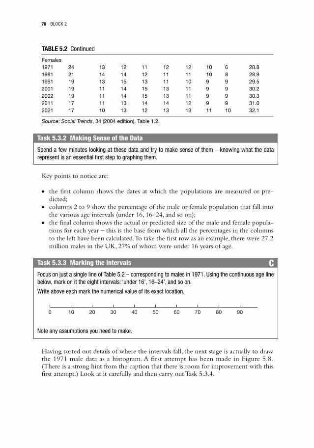
TABLE 5.2 Continued

Females1971 24 13 12 11 12 12 10 6 28.81981 21 14 14 12 11 11 10 8 28.91991 19 13 15 13 11 10 9 9 29.52001 19 11 14 15 13 11 9 9 30.22002 19 11 14 15 13 11 9 9 30.32011 17 11 13 14 14 12 9 9 31.02021 17 10 13 12 13 13 11 10 32.1

Source: Social Trends, 34 (2004 edition), Table 1.2.

Key points to notice are:

� the first column shows the dates at which the populations are measured or pre-dicted;

� columns 2 to 9 show the percentage of the male or female population that fall intothe various age intervals (under 16, 16–24, and so on);

� the final column shows the actual or predicted size of the male and female popula-tions for each year – this is the base from which all the percentages in the columnsto the left have been calculated.To take the first row as an example, there were 27.2million males in the UK, 27% of whom were under 16 years of age.

Having sorted out details of where the intervals fall, the next stage is actually to drawthe 1971 male data as a histogram. A first attempt has been made in Figure 5.8.(There is a strong hint from the caption that there is room for improvement with thisfirst attempt.) Look at it carefully and then carry out Task 5.3.4.

70 BLOCK 2

Task 5.3.2 Making Sense of the Data

Spend a few minutes looking at these data and try to make sense of them – knowing what the datarepresent is an essential first step to graphing them.

Task 5.3.3 Marking the intervals CFocus on just a single line of Table 5.2 – corresponding to males in 1971. Using the continuous age linebelow, mark on it the eight intervals: ‘under 16’, 16–24’, and so on.

Write above each mark the numerical value of its exact location.

Note any assumptions you need to make.

10 20 30 40 50 60 70 80 900

05_CHAP 5.QXD 13/1/06 7:25 am Page 70

The main problem is that columns have been drawn so that the percentages corre-sponding to each interval are proportional to the heights of the columns, rather thanto the areas.When people look at graphs like these, it is to the height of each columnthat their eyes are naturally drawn.As you already know from Task 5.3.3, the intervalwidths are not all equal. In order to ensure a fair comparison based on area of thecolumns, rather than height, the wider columns should be scaled down in height andthe narrower columns scaled up.This can be done using the following two steps:

� identify a convenient basic interval for each column (say, 10 years) as a basis ofcomparison for all the intervals;

� for each interval in turn, calculate the percentage of the population falling into a10-year portion of this interval – this calculation gives the required height of eachcolumn.To take an example, the first column (containing 27% of the population)has an interval of 16 years.You would expect the percentage of the populationfalling into a 10-year portion of this interval to be (10/16) × 27 or roughly 17. So,this is a measure of the correct height to which the first interval should be drawn.

5.4 FLORENCE NIGHTINGALE (1820–1910)

Florence Nightingale’s story is usually portrayed as one woman’s crusade to improvethe quality of life of ordinary soldiers who were dying, needlessly, in their thousandsin Scutari during the Crimean War. But she also needed to convince the authoritiesof the full extent of the scandal of military medical care and encourage them to beprepared to make fundamental changes in the supply of essential medical facilities andto improve the basic hygiene and diet of soldiers in hospital.


0 16 25 35 45Age (years)

55 65 75 95

% o

f pop

ulat

ion

27

14 13 12 12 117

3

Figure 5.8 DODGY HISTOGRAM BASED ON THE POPULATION DATA

Task 5.3.4 Dodgy Histogram

Can you spot the ‘deliberate mistake’ in the drawing of this histogram? How could it be corrected?

Task 5.3.5 Corrected Histogram CBased on the suggestions above, recalculate the correct heights of each column of the histogram andredraw it correctly.

05_CHAP 5.QXD 13/1/06 7:25 am Page 71

She had some useful weapons at her disposal. First, she came from a wealthy upper-class family that moved in the highest echelons of Victorian society. So, when she wasdenied the basic supplies and food that were needed, she could turn for support toinfluential friends like the then Secretary at War, Sidney Herbert. And she also hadprivate means of her own, sometimes having to resort to bypassing the militarybureaucracy by purchasing the supplies she needed out of her own pocket.

But Florence Nightingale’s other weapon was that she was knowledgeable aboutstatistics, and keen to exploit that knowledge. Indeed, she became a formidable andrespected statistician, pioneering a number of original and imaginative measures andforms of graphical representation. She unleashed on a sceptical male military world anarray of well-researched and clearly presented statistics which changed attitudes andallowed fundamental reforms to take place.

She kept and published a careful record of the causes of mortality in British mili-tary hospitals during the Crimean War (1854–56). For example, she showed that, inthe single month of January 1855, 3168 soldiers died in British hospitals. Of these,2889, or just over 90%, died of non-battle causes (mostly cholera and typhus). But shewas not content simply with presenting these data as dry, impersonal numbers. Shewanted them to make a real impact, particularly if they were to be understood by thestatistically unsophisticated, that is, by just about everyone in the mid-nineteenth cen-tury.Table 5.3 shows the data (based on estimates) that she found so shocking.

TABLE 5.3 Florence Nightingale’s data

Date April May June July Aug. Sept. Oct. Nov. Dec. Jan. Feb. Mar.1854 1855

Battle 3 14 19 46 55 86 185 322 138 279 322 169

Non-Battle 28 24 12 396 863 795 367 597 1631 2889 1830 1118

Total 31 38 31 442 918 881 552 919 1769 3168 2152 1287

Just as Minard’s classic chart powerfully captured the loss of Napoleon’s army,Nightingale’s invention of a diagram that she called a ‘coxcomb’ (a kind of lace withan edging like a cock’s comb) did likewise (Figure 5.9). Indeed, she published hercoxcomb diagram along with the phrase,‘the loss of an army’.Today, this form of rep-resentation is known as a ‘polar-area diagram’.

The area of each wedge of the diagram in Figure 5.9 is a measure of the extent ofhospital deaths. Again, to increase the impact of the figures on her audience, largelycomposed of public figures who were untrained in statistical understanding, shedevised a novel way of working it out as a mortality rate.

The number of deaths was given monthly and each month’s figure was expressedas a percentage of the monthly average number of deaths, calculated over the 12months of that year. For example, the monthly average number of non-battle deathsduring 1854 was roughly 879. In January 1855, the actual number of non-battledeaths was 2889, which is 329%, as a percentage of the monthly average.

72 BLOCK 2

Task 5.4.1 Representing Mortality Levels

As you can see, the number of deaths from non-battle causes each month greatly outweighed the cor-responding battle-related deaths. Find a way of representing these figures pictorially so that thesedifferences are very clear, even to a statistical novice (a rough sketch will be sufficient).

05_CHAP 5.QXD 13/1/06 7:25 am Page 72

The main success of this diagram is the (correct) use of area to depict numerical size.Also, the use of two concentric circles is a neat way of seeing two distributions at once.

There are some difficulties with the chart, however. First, it is not clear that the circu-lar arrangement is helpful – although the months of the year are cyclic, that is not animportant issue here and clearly there is nowhere to go after all 12 sectors are in place.Second, her choice to start in the 9 o’clock seems arbitrary and the modern conventionof starting at 12 o’clock seems (at least to modern eyes) to be more natural. Finally, ifher graph is designed to show the benefits of her hygiene reforms, it fails to do sobecause it stops before the results of these reforms took effect.

For comparison, Figure 5.10 shows the same data represented as a componentbar chart.


Oct

Sept

AugustJulyJune

May

Apr 1854

March

February

Jan 1855

From: F. Nightingale, ‘Notes on Matters Affecting the Health,Efficiency and Hospital Adminstration of the British Army’, 1855

Dec

Nov

Non-Battle

Causes of Mortality in the Army in the EastApril, 1854 to March 1855

Battle

Figure 5.9 COXCOMB OR POLAR-AREA DIAGRAMSource: www.math.yorku.ca/SCS/Gallery/noframes.html

Task 5.4.2 Summarising the Coxcomb C(a) Spend a few minutes studying Figure 5.9 to gain an understanding of the patterns of death levels

over this 12-month period.

(b) Bearing in mind some of the issues raised in Section 5.2, how successfully do you thinkNightingale’s diagram depicts these data to make the point that she wished to get across? In par-ticular, do you feel that the circular arrangement is helpful?

05_CHAP 5.QXD 13/1/06 7:25 am Page 73

Between October 1854 and January 1855, just three months later, the levels of mor-tality had increased by a factor of six. Her sanitary reforms went into operation inMarch 1855. By the late spring, mortality levels had dropped to something like onetwentieth of the level a few months earlier.

In defiance of the military authorities, Florence Nightingale published data andanalyses such as these.The statistical sections of her reports, normally relegated todusty shelves, she printed off separately and circulated them to every Member ofParliament. It was the power of her data, combined with the intuitive simplicity ofthe calculations and graphical representations that she herself devised – as well, ofcourse, as her political shrewdness – that brought these sorts of data, and the needlessdeaths they described, to life in the public consciousness.

In fact, the coxcomb was Nightingale’s second attempt at comparing areas in thisway.The first, which she referred to as a ‘bat’s wing’, was drawn such that the length ofeach radial line was proportional to the mortality levels.This was misleading, since theeye is naturally drawn to comparing areas. Nightingale recognised her error (afterpublication) and felt obliged to include an erratum note.

Florence Nightingale took the view that the ruling classes of Victorian England(both those in the military hierarchy and in government) were either unwilling orunable to see the truth about conditions in Scutari and elsewhere unless presented withirrefutable evidence. Her life's work as a statistician, therefore, centred around two key

74 BLOCK 2

April1854

May0

500

1000

1500

2000

2500

3000

3500

June July Aug Sept

Month

Dea

ths

Oct Nov Dec Jan1855

Feb Mar

Non-Battle

Battle

Figure 5.10 NIGHTINGALE’S DATA REPRESENTED AS A COMPONENT BAR CHART

Task 5.4.3 Investigating the Coxcomb CIt is not a good idea to assume that a particular graph always provides a fair representation of the data.To test out the coxcomb, measure as accurately as you can with a ruler the radii of the October 1854and January 1855 wedges of the coxcomb. Using a suitable calculation, check the claim above thatthese wedges show an increase in mortality by a factor of about six over this three-month period.

05_CHAP 5.QXD 13/1/06 7:25 am Page 74

themes. First, she needed data that she could trust.The data had to be accurate, compre-hensive and comparable between hospitals and between regions.This resulted in herlong-running campaign to standardise hospital record-keeping. Second, she was awarethat most of the decision-makers around her were statistically illiterate and tables of fig-ures, however accurate, were simply not winning over their hearts and minds.This ledher to devise creative and innovative forms of diagrammatic and graphical representa-tions of her data, which demonstrated the underlying patterns in a way that no onecould ignore. For a readable account of these issues, see Cohen (1984).

5.5 PEDAGOGY

As usual, this section on teaching and learning issues asks you to carry out tasks basedon the six PTT themes.

Language Patterns

Imagery

Different Contexts

Learners only need to flick through a newspaper or magazine or to watch a currentaffairs programme on television to see a range of statistical graphs and charts. Clearly,there is scope for incorporating some of these into statistical lessons, in the context oftrying to make sense of someone else’s statistical picture.The other side of this coin isfor learners to use statistical pictures in order to represent their own data.


Task 5.5.1 Words C(a) Make a list of the key statistical words and phrases that were used in this chapter.

(b) With a particular learner or group of learners in mind, decide which of these words and phrases itwould be appropriate for them to know.

(c) How might you help them gain a better understanding of these ideas?

Task 5.5.2 People Graphs CA simple but effective way of illustrating the nature of a bar chart is to create a people graph, as fol-lows. Ask a group of children to sort themselves, say, by hair colour (dark, brown, fair, red). A bar chartcan be formed if they stand, equally spaced in four parallel rows. How might this idea be extended toform a pie chart?

Decide for what age of learners creating people graphs could be an effective teaching strategy. Howwould you bridge the gap between a people chart and one drawn on paper?

Choose one of the other graphics covered in this chapter. How might you use ‘visualising’ to clarify thekey ideas to learners?

05_CHAP 5.QXD 13/1/06 7:25 am Page 75

For example, Rosie’s passion ismusic and, in particular, using heriPod MP3 player. With her musicstored on a computer, she caninstantly identify the various genresof music in her collection and thenumber of artists within each genre.Figure 5.11 is a pie chart represent-ing Rosie’s music collection, bymusical genre. At a glance, she canuse the chart to gain an insight intoher musical tastes.

Root Questions

76 BLOCK 2

Rosie's Recordings

Pop52%

Rock25%

R&B12%

Folk11%

Figure 5.11 A PIE CHART OF ROSIE’S RECORD COLLECTION

Task 5.5.3 A passion for Pie Charts C(a) Rosie’s pie chart depicts the number of separate tracks in her collection that fall into each category.

How else might the pie chart categories be organised?

(b) Make a short list of other contexts that your particular groups of learners might find motivating.

(c) Choose two of the graphics described in this chapter and sketch possible graphics that might arisewithin the contexts you have identified.

Task 5.5.4 Words Versus Pictures

Section 5.1 ended with four key features that characterise a well-designed graphic. Here are oneperson's notes for an activity designed to convey this in an interesting manner:

• set up a competition called ‘words versus pictures’;

• one learner is asked to convey certain information in words using, say, less than 100 words;

• a second learner must depict the same information using a graphic representation plus a maximumof five words for titles and labelling;

• the two representations are compared and other learners decide which is ‘better’ and why;

• follow up with a discussion of the strengths and weaknesses of each approach.

For what age of learner is this task appropriate? Bullet point 2 talks of ‘certain information’. Decide ontwo different pieces of information that would be appropriate to use and decide how this informationcould be presented.

05_CHAP 5.QXD 13/1/06 7:25 am Page 76




Task 5.5.5 Getting it Wrong CBearing in mind the content of this chapter and the particular learner(s) you have in mind, choose atopic that you think may be the basis of a learner misconception (or perhaps a ‘partial conception’). Tryto explain the misconception, why it may occur and how you might try to remedy it.

Task 5.5.6 Made by Hand CA feature of data presentation with a computer is that it is achieved with just a few clicks of the mouse.Drawing a graphic by hand demands some technical skill and may take a long time. A key pedagogicissue is how long to spend on the various methods of creating graphics.

(a) List the technical skills that your learners would need if they were to be able to create a pie chartwithout a computer. What are the gains and losses if they were only to use a computer instead?

(b) Choose another graphic from this chapter and repeat (a).

05_CHAP 5.QXD 13/1/06 7:25 am Page 77

6 Comparing with Pictures

This chapter offers a second opportunity for you to think about questions of compar-ison in statistics. In Chapter 2, you considered this idea based on using words andnumbers – now it is applied to pictures. One of the ‘big ideas’ of statistics, highlightedin Chapter 2, was the following root question that underpins many statistical investi-gations:‘Is A bigger than B?’ Here are some examples:

� ‘Are pupils faster than teachers at texting with mobile phones?’� ‘Is traffic heavier on a Saturday than a Sunday?’� ‘Are people’s speed of reaction faster using their dominant hand than their non-

dominant hand?’� ‘Are girls better able to distinguish colours than boys?’

At an advanced level of statistical work, there are certain formal tests that are used tomake comparisons between two data sets – for example, the z-test, the t-test, the chi-squared test, and so on. However, these are beyond the scope of this book and anotherway must be found to answer questions of comparison.An acceptable alternative is todepict the two data sets graphically and then make visual comparisons.Two graphicsthat are particularly good for comparing sets of data are the box plot and the stemplot and these are examined in Sections 6.2 and 6.3. Section 6.4 asks you to workthrough a statistical investigation based on comparing writing styles. The chapterends, as usual, with a section on pedagogy.

The first section looks at some examples of how a well-chosen graphic can create aparticular impression.

6.1 GETTING THE MESSAGE ACROSS

In a Brooklyn courthouse in 1987, alleged Mafia godfather John Gotti (known as the‘dapper don’; Figure 6.1), along with his six co-defendants, was tried on and acquittedof racketeering and conspiracy charges.The failure to convictafter a widely reported, seven-month trial was a serious blow tothe US government’s campaign against organised crime.

A key factor in securing Gotti’s release was the final exhibit(Table 6.1) prepared by Gotti’s defence team and handed to thejury just before they retired to make their decision. It was a chartlisting the names of the seven key witnesses who had testifiedagainst Gotti and the various crimes of which these witnesses hadthemselves been convicted. Study Table 6.1 for a few minutes andthen try Task 6.1.1.

Figure 6.1 JOHN GOTTI (1940–2002)Source: The New York Times Agency

06_CHAP 6.QXD 13/1/06 7:26 am Page 78

Now You See It

TABLE 6.1 The criminal activity of seven witnesses

Criminal activity of government informants

Crime Cardinale Lofaro Maloney Polisi Senatore Foronjy Curro

Murder X XAttempted murder X X

Heroin possession and sale X X X XCocaine possession and sale X X X

Marijuana possession and sale XGambling business X X X

Armed robberies X X X X XLoansharking X X

Kidnapping X XExtortion X X

Assault X X X XPossession of dangerous X X X X X X

weapons

Perjury X XCounterfeiting X XBank robbery X X

Armed Hijacking X XStolen financial documents X X X

Tax evasion X XBurglaries X X X X

Bribery X XTheft: auto, money, other X X X X XBail jumping and escape X X

Insurance frauds X XForgeries X X

Pistol whipping a priest XSexual assault on minor XReckless endangerment X

Task 6.1.1 Creating a Bad Impression C(a) Without thinking about it for more than a few seconds, estimate, roughly, the percentage of boxes

that are marked with an X.

(b) Look at the order of the criminal activities shown down the left of the table. How do you think thesehave been ordered?

(c) What overall impression does this table convey?

COMPARING WITH PICTURES 79

Task 6.1.2 Don’t Blame the Drink! CLook at the glass of wine below in Figure 6.2. Make a rough estimate of what percentage of the glassis filled.

06_CHAP 6.QXD 13/1/06 7:27 am Page 79

To check your estimate, a calculation canbe made to find the ratio of the volume ofwine in the glass to the maximum capacityof the glass. Both of these are roughly con-ical in shape, so you need to know that theformula for the volume of a cone is(4/3)πr2h, where r is the radius of the cir-cular ‘base’ of the cone and h is its height.

If you measure the level of the wine as apercentage of the total depth of the glass, itis roughly 80% of the way up the glass.Correspondingly, the radius of the circularwine surface is also 80% of the radius ofthe circular top of the glass. So, applying the formula for the volume of a cone, theratios of the volume of wine to maximum capacity of the glass is determined bysquaring the ratio of the radii and multiplying by the ratio of the heights. (Note that,when computing these ratios, the constants 4/3 and π cancel out.) In other words,the volume ratio is found by calculating (0.8)3 = 0.512, which is roughly one half.

A fundamental way in which pictures change real-ity is that when any image (such as this photograph ofthe wine glass) is printed on a page, the three-dimen-sional world that it represents collapses into twodimensions. Inevitably, therefore, comparisons such asthe one presented in Task 6.1.2 will be misleading.Since only two dimensions are available on a printedpage, the eye tends to compare areas, not volumes.

To illustrate this point, the shaded triangle inFigure 6.3 represents half the area of the total trian-gle. If you measure the heights of the triangles, youwill find that the shaded triangle is roughly 70% ofthe height of the larger one, not 80% as it was in the three-dimensional (3-D) case.So, that is why this particular ‘glass’ does look roughly half-full, even though, as a pic-ture of a 3-D glass, it would be only (0.7)3, or roughly 35% full.

Cleverly drawn pictures can sometimes disguise or render invisible what is there.Atother times, they can make you see things that are not really there. It is helpful to beaware of how these illusions are achieved, as some of the illusionist’s ‘tricks of thetrade’ can also be found in distortions used in graphs and diagrams.

6.2 EXPLORATORY DATA ANALYSIS (EDA)

John Wilder Tukey (Figure 6.4) was born in New Bedford,Massachusetts, in 1915. He gained degrees in chemistry, fol-lowed by a doctorate in mathematics and, from 1939 on,taught mathematics at Princeton University. He directedPrinceton’s Statistical Techniques Research Group from itsfounding in 1956.

Although internationally known for his studies in mathe-matical and theoretical statistics and their applications,Tukey led

80 BLOCK 2

Figure 6.2 A GLASS OF RED WINE

Figure 6.3 A DRAWING OF AGLASS OF RED WINE

Figure 6.4 JOHN TUKEY (1915–2000)Source: stat.bell-labs.com/who/tukey/

06_CHAP 6.QXD 13/1/06 1:19 pm Page 80

the way in the field of Exploratory Data Analysis (EDA).The seminal work in EDA isTukey (1977). Exploratory Data Analysis is more than just a collection of data-analysistechniques; it provides a philosophy of how to dissect a data set. It stresses the powerof visualisation and aspects such as what to look for, how to look for it and how tointerpret the information it contains. Most EDA techniques are graphical in nature,because the main aim of EDA is to explore data in an open-minded way. Usinggraphics, rather than calculations, keeps open possibilities of spotting interesting pat-terns or anomalies that would not be apparent with a calculation (where assumptionsand decisions about the nature of the data tend to be made in advance).

Although bar charts, pie charts and histograms have been around for a long time,the EDA movement brought with it a number of exciting new ways of visualising datathat are gradually becoming established in school and college statistics syllabusesaround the world.Whereas traditional approaches to data analysis emphasised the meanas the key measure of location and the standard deviation as the fundamental measureof spread, EDA stresses the median and the interquartile range respectively. Note thatthese summary measures are not the result of performing an abstract calculation, butare based on picking out particular values from the set, when sorted in order of size.Akey feature of visualisation, in EDA terms, is imagining the data items laid out on anumber line (or in a series of rows) and matching this to a helpful graphic.

You have already seen in Chapter 2 an example of a visualising technique that isnormally attributed to EDA – the five-figure summary. In this chapter, you will lookat two further examples: the box plot (also known as the box-and-whisker diagram) andthe stem plot (also known as the stem-and-leaf diagram).They have been included in thischapter because they not only provide excellent ways of summarising single sets ofdata, but also offer particularly powerful ways of comparing two or more data sets.

Box Plots

A box plot is a simple but powerful means of gaining an overview of a set of data bymarking, on a number line, the five key summary statistics: Min, Q1, Med, Q3 andMax. For example, here are the examination scores (in order) of 14 students.

23, 35, 41, 45, 55, 55, 58, 60, 62, 66, 69, 72, 73, 73.

The summaries (as calculated both by the calculator and by Tukey’s method) are:

Min = 23, Q1 = 45, Q2 = 59, Q3 = 69, Max = 73.

In Task 6.2.1, you are asked to go through the main steps of translating these sum-maries into a box plot.

The box plot shows the locations of the quarter points of the data.The left and rightwhiskers correspond, respectively, to the values of the bottom and top quarters of thevalues, the central box corresponds to the values of the middle 50% of the values and


Task 6.2.1 Creating a Box with Whiskers CImagine that you are working with students who require detailed instructions on how to draw a boxplot. Using the example of the data set of 14 marks above, write down the main steps, suitable for anaudience of your choosing.

06_CHAP 6.QXD 13/1/06 7:27 am Page 81

82 BLOCK 2

the median line separates these into the second and third quarters of the data.Thestrength of this diagram is that you can see at a glance where these five key summariesfall in relation to each other and thereby gain a useful visualisation of the overall dis-tribution of values. For instance, in this example, the right whisker is shorter than theleft one, and the right portion of the box is shorter than the left.

It is when two or more data sets are to be compared that box plots really come intotheir own. Consider the data sets below, which were collected from a class project ontexting speeds. A group of Key Stage 3 (KS3) students challenged their teachers to aspeed-texting competition.The 21 participants (12 students and 9 teachers) were eachrequired to send a short text message on a mobile phone.Their times and the sum-maries for each group (Table 6.2) are given below. For convenience, the data havebeen sorted in order of size.

Teacher times (secs): 18, 27, 28, 31, 33, 33, 36, 47, 51.Student times (secs): 19, 19, 21, 24, 24, 25, 27, 29, 30, 30, 33, 41.

It is clear from the completed box plots that the students’ times are generally fasterthan those of the teachers.The only redeeming feature of the teachers’ performancewas their one exceptionally fast time of 18 seconds, but for all the other four summaryvalues, the students outperformed them. In fact, the median student time (26 seconds)

Task 6.2.2 The Long and the Short of a Box Plot CThink about the implications of a lack of symmetry in a box plot in terms of where the data values areconcentrated.

For cases where the left whisker is longer than the right whisker, are either of the following statementstrue?� Values are more densely packed into the bottom 25% than the top 25% of the batch.� Values are more densely packed into the top 25% than the bottom 25% of the batch.

TABLE 6.2 Student and teacher summaries

Min Q1 Med Q3 Max

Teachers 18 27.5 33 41.5 51Students 19 22.5 26 30 41

Task 6.2.3 Box Plots Compared C(a) What inaccuracies do you think might have cropped up in this experiment and how might they have

been dealt with?

(b) Sketch two box plots, one above the other, for the teacher and student times. Make sure that bothplots relate to the same horizontal scale.

(c) Comparing the two box plots, what can you conclude about the relative performances of the teach-ers and the students?

06_CHAP 6.QXD 13/1/06 7:27 am Page 82


was actually faster than the lower quartile teacher time (27.5 seconds). Put anotherway, half of the students were faster than the best quarter of the teachers. Also, theworst performing student (timed at 41 seconds) performed better than the slowestquarter of the teachers (the fastest of these apparently being shown at 41.5 seconds, butrecall that this Q3 figure is actually a computed average of 36 and 47 seconds).

Deciding on Differences

In Task 6.2.3, you were asked to compare, visually, the student and teacher box plots.Clearly, student times are, overall, faster than those of their teachers, but there wasquite wide variation in the two sets of times and therefore considerable overlapbetween the two box plots. When comparing two sets of data in order to decidewhether or not there is a difference, two key factors need to be considered – whetherthere is a difference in the location of the two data sets and how widely the two sets ofvalues are spread.

Imagine two schools, A and B, where a similar experiment on measuring textingspeeds was carried out. In both schools, the difference in location between studentand teacher times was very similar to the data above (with medians of 26 and 33,respectively), but the spreads were very different.

These are represented by the two pairs of box plots (Figure 6.5).

The differences are more convincing in school B, where the spreads are small. In gen-eral, differences are more convincing when the locations differ widely and the spreadsare narrow.

Figure 6.5 TEACHER AND STUDENT BOX PLOTS FROM TWO SCHOOLS

Task 6.2.4 Location and Spread

(a) For which of these schools, A or B, would you feel able to claim with greater confidence that thestudents have outperformed the teachers?

(b) In general, when comparing two sets of data, how do their locations and spreads affect your judge-ment when deciding on differences?

(c) Can you think about a third factor (as well as location and spread) that might affect the process ofdeciding on differences?

06_CHAP 6.QXD 13/1/06 7:27 am Page 83

84 BLOCK 2

A relevant third factor is the batch size.The larger the batch size, the more confi-dent you can be that the shape and position of the box plot has settled down.Where,say, just five or six values are plotted, these may be fairly unrepresentative of the wholebatch and the shape and position of the box plot may change considerably as moredata are collected.

In summary, then, when deciding on differences between two data batches, youneed to look for:

� a large difference in location;� small spreads in the batches;� large batch sizes.

As was mentioned at the beginning of this chapter, students under the age of 16 arenot expected to make use of formal tests of significance.When deciding on differ-ences, therefore, these students must look elsewhere to inform their decision-making.One alternative is to perform relevant calculations (for example, averages) and makenumerical comparisons.The alternative explored here is to make visual comparisonsbased on helpful graphics such as box plots. However, where students are makingvisual comparisons, they should be aware of the relevance of location, spread andbatch sizes to inform their interpretation. Another option to consider is the creationof several samples.This is easier to achieve by means of simulations using a computeror graphics calculator, something that is explored in Block 3.

6.3 STEM PLOTS (OR STEM-AND-LEAF DIAGRAMS)

Another visual representation attributed to John Tukey and the EDA movement is thestem plot (also known as the stem-and-leaf diagram). Task 6.3.1 asks you to thinkthrough the procedure of drawing a stem plot based on the data you used in the pre-vious section. For convenience, the data are repeated below.

Student times (secs): 19, 19, 21, 24, 24, 25, 27, 29, 30, 30, 33, 41.Teacher times (secs): 18, 27, 28, 31, 33, 33, 36, 47, 51.

The students’ completed stem plot should look like this.

0|1|992|1445793|0034|15|

1|9 means 19

Task 6.3.1 Creating a Stem-and-leaf Diagram CImagine that you are working with students who require detailed instructions on how to draw a stemplot. Using the example of the student and teacher times above, write down the main steps, suitable foran audience of your choosing.

06_CHAP 6.QXD 13/1/06 7:27 am Page 84

Note that, in this example, as shown in the ‘key’ at the bottom, the tens correspondto the stem, while the unit parts of the numbers are the leaves. Conventionally, theleaves are placed in increasing order of size along each branch corresponding to the‘tens’ branch to which they are linked.When teaching stem plots to older students, anumber of deeper questions may arise and you are asked to think about some of thesein Task 6.3.2.

A useful feature of a stem plot is that the values maintain their natural order, while atthe same time they are laid out in a way that emphasises the overall distribution ofwhere the values are concentrated (that is, where the longer branches are). Thisenables you easily to pick out key values such as the median and quartiles.

Comparing Stem Plots

Just as box plots are a good way of comparing two data sets, so too are stem plots.However, this is not done with one placed above the other (as is the case when com-paring two box plots), but rather with them placed back-to-back.This is illustrated inFigure 6.6.


Task 6.3.2 Deeper Questions about a Stem Plot C(a) Unlike the box plot or histogram, a stem plot incorporates and displays each separate data value.

What are the advantages and disadvantages of this feature?

(b) What other features does a stem plot share with a box plot and a histogram?

(c) Is it important that the values on each branch are ordered?

(d) What are some advantages and disadvantages of the convention of drawing a stem plot so that thevalues on the stem increase downwards?

Task 6.3.3 Interpreting the Stem Plot CFrom the stem plot based on student times, pick out the Min, Max and Med values.

Teacher times (secs) Student times (secs)

8

87

6331

7

1

0

1

2

3

4

5

99

144579

003

1

Figure 6.6 A BACK-TO-BACK STEM PLOT

4 |1 means 41

06_CHAP 6.QXD 13/1/06 7:27 am Page 85

With a back-to-back stem plot, you can compare, at a glance, the extreme values ofthe two data sets. Also, as has already been observed, the length of each branch is agood indication of where the values are concentrated. So, this allows you to seeimmediately that the modal interval for the students is 20–29 seconds, whereas for theteachers it is 30–39 seconds.

As was mentioned in the comments to Task 6.3.2, a stem plot is very similar to ahistogram with equal class intervals, except that the picture has been turned through90º.Thus, all the interpretations afforded by a histogram are also available with a stemplot, with the added advantage that two sets of data can now be compared directly.

The particular data sets used here were easy to display as a stem plot – eachnumber consisted of two digits, so naturally the ‘tens’ digit formed the stem and the‘units’ digit filled the leaves. Data are not always so co-operative and sometimes youwill need to be a little creative when displaying the numbers in a stem plot, as youwill see in the next task.

Ideally, the optimum number of branches on a stem plot should be somewherebetween four and eight.With small data sets, anything more or less than that makes ithard to perceive any underlying shape to the distribution.With this first data set,something unconventional may be required, such as grouping the data in twos.Thistime, the stem value marked 4 refers to the range 4–5, not 40–49.

The final stem plot will look something like this.

2|24|445556|667778|889

8|9 means 9Note that the key is particularly important here as 8|9 is more conventionally

taken to mean something like 89 or 0.89.You may take the view that this particularform of stem plot is so unconventional as to be confusing for students.An alternativeapproach might be to use a dot plot, with dots corresponding to 8, 9, and so on, asshown in Figure 6.7.

86 BLOCK 2

Task 6.3.5 Making the Data Fit the Stem Plot

Making whatever adjustments you feel necessary, display the two data sets below as separate stemplots.

2, 4, 4, 5, 5, 5, 6, 6, 7, 7, 7, 8, 8, 9.

431, 506, 544, 582, 610, 627, 674, 711, 729.

Can you come up with a sensible general rule for creating a stem on a stem plot?

Task 6.3.4 Interpreting the Back-to-back Stem Plot

(a) What features can be compared using a back-to-back stem plot?

(b) What similarities can you observe between this representation and others, such as a histogram?

06_CHAP 6.QXD 13/1/06 7:27 am Page 86

Whereas with the first data set, each item had too few digits to make a conven-tional stem plot, the second set had the opposite problem.The simplest solution is toround each value to two figures, thus:

430, 510, 540, 580, 610, 630, 670, 710, 730.

You can then make the plot using the hundreds digits as the stems and the tens digitsas the leaves, as follows.

4|35|1486|1377|13

7|1 means 710To end this section, Figure 6.8 contains a timetable that has been used by Japanese

rail passengers for many years (and probably all were quite unaware of the term ‘back-to-back stem plot’).

The central stem corresponds to hours, while the leaves are arranged as pairs ofdigits, corresponding to minutes.The left half of the schedules refers to platforms 7and 8, while the right half refers to platforms 5 and 6. Note also that time increasesdownwards on the vertical stem.


1 2 3 4 5 6 7 8 9

Figure 6.7 DOT PLOT SHOWING THE FIRST DATA SET FROM TASK 6.3.5

Figure 6.8 TOKAIDO LINE AT YOKOHAMA STATION (SAGAMI TETSUDO COMPANY, 1985 TIMETABLE, P. 72)Source: Tufte (1990, p. 47).

06_CHAP 6.QXD 13/1/06 7:27 am Page 87

6.4 A STATISTICAL INVESTIGATION ON COMPARING

In this section, you are asked to carry out a statistical investigation, comparing thewriting of three authors, Jane Austin, J.K. Rowling and J.R.R.Tolkien. Clearly, thereare many subtle features that characterise particular authors’ styles – for example, theiruse of metaphor, description, imagery, and so on – but here you are simply asked toconcentrate on writing characteristics that are easily defined and measured. As youtackle this investigation, notice that it has been organised into the four key stagesintroduced in Block 1 that mark out the thinking required in order to conduct a sta-tistical investigation. (These are also described in the Key Stages 3 and 4 Programmesof Study in England.) The stages are Pose the question, Collect relevant data, Analysethe data and Interpret the results (summarised as PCAI).Throughout this book, otherinvestigations are offered for you to try and these are also organised using these fourheadings.A more general discussion on issues relating to conducting a statistical inves-tigation appears in Chapter 14.

The P Stage – Pose the Question

Posing a suitable or sensible question is a crucial part of the PCAI data-handlingcycle, since it is the key to everything that follows in the investigation. Students willnot find this initial step easy, particularly if they have not had much previous experi-ence of working investigatively. Ensuring that each student has a sense of individualchoice and personal ownership of the investigation will be important. But, at thesame time, the teacher will not want them to embark on an extended piece of workthat is likely to fail. Consequently, considerable teaching skill and tact will be requiredto help them move from a vague, general idea to formulating a realistic question thatcan be investigated.

Here are five considerations that might help students to come up with a goodquestion for investigation. Choose a question that is:

� actually a question, rather than simply an area for investigation – an investigationbased on a question is more likely to draw on statistical and mathematical skills andprovide greater focus and clearer direction;

� personally interesting to you – not only will this bring greater motivation, but alsoyour common-sense knowledge about the context should help ensure that theinvestigation proceeds along sensible lines;

� likely to draw on data that will be available within the time frame of the investiga-tion – for example, do not investigate the growth of flowers or plants during thewinter months;

� specific, so that it is answerable from data – questions that are too vague and gen-eral are harder to answer;

� measurable – think through in advance what you will measure and whether it willhelp to answer the question.

In general, it is useful for students to be familiar with the PCAI cycle when they areat the question-posing stage. A useful exercise when first selecting a question is forthem to go through in their minds how the investigation might develop at the subse-quent C, A and I stages. If they can foresee a stumbling block, this might be becauseof some problem in the wording of the investigation, in which case they can try tocome up with a rewording that gets around the problem.

88 BLOCK 2

06_CHAP 6.QXD 13/1/06 7:27 am Page 88

In this section, you are asked to follow through a short investigation based on thequestion: ‘Which of the authors writes the simplest sentences?’ Before thinking aboutcollecting relevant data, note down your instinctive response to this question.Thiswill make it more interesting when you reach the final stage of your investigation andyou can compare what you found with what you expected.

The C Stage – Collect the Data

How can you measure the complexity of the sentences written by different authors?One simple approach would be to take a sample of, say, 30 sentences from eachauthor and count the number of words in each sentence. A possible weakness of thisapproach is that it does not take word length into account. Both of these factors, thenumber of words and word length, can be compounded by counting, say, the numberof letters per sentence or even the number of syllables.The latter approach is the oneyou are asked to take here.

The books selected were:

Pride and Prejudice (by Jane Austen)Harry Potter and the Goblet of Fire (by J.K. Rowling)Lord of the Rings:The Two Towers (by J.R.R.Tolkien)

The next choice is how to select the sentences from these books.

There are other measuring choices to be made when measuring sentence length,whether you are counting words, syllables or letters. For example, the ambiguities ofpronunciation sometimes make it difficult to know precisely how many syllables arein each word. Where letters are being counted, rather than syllables, you need todecide whether or not to include punctuation marks and spaces between words.

Table 6.3 shows the syllable lengths of 30 randomly chosen sentences from thesethree books. In the next sub-section, you are asked to analyse these data visually.

The A Stage – Analyse the Data

As you may have already guessed from the way the data have been presented, theywere entered into a spreadsheet.The eight relevant summary statistics (Mean, Range,IQR, Min, Q1, Median, Q3 and Max) for the Austen and Tolkien data were calcu-lated and are displayed in Table 6.4.


Task 6.4.1 Choosing the Right Question CThink about the general area of this investigation (comparing authorship) and write down as preciselyas you can two or three questions that you feel would be both interesting and also answerable by stu-dents below the age of 16. Bear in mind the C, A and I stages that are likely to follow, and adjust thewording of your questions accordingly.

Task 6.4.2 Selecting the Sentences CConsider several ways of selecting the sentences and weigh up their advantages and disadvantages interms of collecting the data fairly.

06_CHAP 6.QXD 13/1/06 7:27 am Page 89

90 BLOCK 2

Producing these summaries is an important step at the A stage of an investigationand one that is greatly supported by ICT. Information and communication technol-ogy can also support creating helpful visual representations of the data, something youwill look at again more closely in Block 3.

TABLE 6.3 Syllable lengths from sentences of three authors

Austen Rowling Tolkien

1 50 26 332 63 12 333 9 42 44 10 26 25 37 23 66 8 62 77 33 27 148 46 80 159 30 44 10

10 34 42 1811 38 67 1412 50 73 2813 39 35 1314 10 64 615 60 30 1616 68 10 6217 50 13 1718 54 34 4019 30 20 420 16 17 1121 78 54 522 136 31 1023 57 42 4424 12 29 4525 10 26 926 59 40 2927 8 37 1428 30 28 1029 49 13 830 79 52 7

TABLE 6.4 Eight summary statistics for Austen and Tolkien

Austen Tolkien

Mean 41.8 17.8Range 128 60IQR 36.8 18.3

Min 8 2Q1 19.5 7.3Median 38.5 13.5Q3 56.3 25.5Max 136 62

06_CHAP 6.QXD 13/1/06 7:27 am Page 90


The I Stage – Interpret the Results

The final stage of the investigation is to interpret the results produced in the A stage.

6.5 PEDAGOGY

As usual, in this section on teaching and learning issues, you are asked to carry outtasks based on the six PTT themes.

Language Patterns

Imagery

Different Contexts

Task 6.4.3 Visualising the Data CRepresent, visually, the Jane Austen and J.R.R. Tolkien data, in order to compare their levels of difficulty(to save time, a rough sketch will be sufficient here). How fairly does your choice of representationdescribe the data sets overall?

Task 6.4.4 Interpreting the Box Plots C(a) Based on the summaries and box plots, what can you conclude about these two authors, Jane

Austen and J.R.R. Tolkien?

(b) You have now completed one complete pass around the PCAI cycle. This does not necessarily meanthat you have completed the investigation. What further thoughts or ideas do you have?

(c) If you have time, you could carry out a similar investigation based on the Rowling data, starting withyour intuitive guess as to how her sentence lengths would compare with these other two authors.

Task 6.5.1 The Long and the Short of it CThe terms ‘box plot’ and ‘box-and-whisker diagram’ were used to describe the same representation.This is also true of the terms ‘stem plot’ and ‘stem-and-leaf diagram’. What are some advantages anddisadvantages of using these different terms with learners?

Task 6.5.2 People Plots CRecall how, in Task 5.5.2, people graphs were suggested as means of visualising vividly both bar chartsand pie charts. Can you think of similar activities to illustrate box-and-whisker and stem-and-leaf dia-grams? Consider, for example, an investigation where each student has recorded the number ofseconds it took them to send a (standard) text message.

Task 6.5.3 Sporty Plots CMany people are interested in sport. With a particular learner or group of learners in mind, think ofexamples from sporting contexts where box-and-whisker and/or stem-and-leaf diagrams would beuseful to make comparisons between sets of data.

06_CHAP 6.QXD 13/1/06 7:27 am Page 91

Root Questions



In this chapter, box plots and stem plots have been suggested as means of comparing datasets. In Chapter 5, bar charts, histograms and pie charts were discussed and, of course,these diagrams too can be used to make visual comparisons of sets of data. For example,two pie charts can be placed side by side or compound or component bar charts (theseare explained in Block 3) can be used to compare more than one attribute at a time.

With such a variety of types of charts available, it is not easy to decide which to usein any particular instance. A list of the factors that influence your choice couldinclude the following:

� some are much easier than others to draw by hand;� a stem plot is good for numerical data in the range 0–99, where the stem and

leaves correspond, respectively, to tens and units. It is less satisfactory for more awk-ward decimals, where the meaning of the stem and the leaves is not so obvious.Also, stem plots are not useful for large data sets.

92 BLOCK 2

Task 6.5.4 Root Question CConsider the term ‘difference’ as it might be used in statistics.

Make a note of a possible root question that connects it to ideas of natural variation.

Task 6.5.5 Symmetrical Box Plots?

a) Recall the box plot produced in Task 6.2.1. Imagine that one of your students produced the box plot inFigure 6.9 from the same data. In fact, all the box plots they produce show the same perfect symmetry.What fundamental misconception do you think they might have? How you might try to remedy it?

b) Bearing in mind the content of this chapter and the particular learner(s) you have in mind, writedown some possible misconceptions. For each misconception you can think of, describe how you,the teacher, would become aware of it and how you might remedy it.

0 20 40 60 80 100

Figure 6.9 A SYMMETRIC BOX PLOT

Task 6.5.6 Comparing Charts of Comparison C(a) Make as full a list as you can of other factors that might affect your choice when you want to make

a visual comparison of data sets.

(b) Is this task a good one for your students to carry out?

06_CHAP 6.QXD 13/1/06 7:27 am Page 92

7 Interrelating with Pictures

Chapter 6 was about looking for differences between attributes (for example, ‘menversus women’, ‘children versus adults’, and so on). The information required toanswer such questions were two sets of numerical data, one for each attribute. Nowconsider the following question that might be the subject of a class investigation:‘Canpeople with longer legs run faster?’

There are two possible approaches to tackling a question like this. One is to adaptit to match the approach taken in Chapter 6, by creating two groups of people (’thelong-legged’ and ‘the short-legged’) and then measuring their respective runningspeeds. (Note that the two batches do not need to be of equal size.) The data for thesetwo data sets could then be compared numerically using averages or visually usingbox plots or stem plots.

However, this classification of people into two leg lengths creates rather an artificialdistinction. Leg length is not an attribute like ‘gender’ or ‘hand dominance’, but a full-blown variable with all the features of a ratio scale.The second approach, the onefeatured in this chapter, is to acknowledge that leg length and running speed are bothvariables.This will mean using paired (that is, bi-variate) data in order to explore therelationship between them. In Chapter 3, you looked at such relationships in terms ofwords and pictures. Here you will look at the power of pictures (particularly scatterplots and line graphs) to explore such relationships.

A particularly common example of interrelating can be seen in time series plots –that is, tables or graphs showing how some quantity (say, height, weight, earnings,sales, and so on) changes over time.A feature of time series graphs is that the variable‘time’ is always placed on the horizontal axis, for the simple reason that time is alwaysthe ‘explanatory’ variable in such situations.

Section 7.1 looks at some of the data that can be found on the CensusAtSchoolwebsite and examines how such data can be made the basis of an ‘interrelating’ inves-tigation. Sections 7.2 and 7.3 consider ideas of regression and correlation. Section 7.4provides examples of ways in which pictures can misrepresent data, while the finalsection looks at pedagogic issues.

7.1 THE CENSUSATSCHOOL DATA SOURCE

In this section, you are asked to look at some possible school-level investigationsbased on data found at the CensusAtSchool website: www.censusatschool.ntu.ac.ukThe CensusAtSchool project is run by the Royal Statistical Society Centre forStatistical Education, based at Nottingham Trent University. It is an international chil-dren’s census set up to collect and disseminate real data for use by teachers and pupils

07_CHAP 7.QXD 13/1/06 7:27 am Page 93

in data handling, ICT and projects across the curriculum. Countries currently repre-sented are UK, South Africa, Australia, New Zealand and Canada.You will have theopportunity to look at this site more closely in Block 3 and use it as it has beendesigned to be used, namely, supported by ICT.

Table 7.1 contains a small selection of the many thousands of data items available atthis site.These 20 boys and girls were aged 11 to 14 years and all measurements pro-vided are in centimetres.

The graphs in Figure 7.1 were drawn from Table 7.1. Note that they have been delib-erately left unlabelled in order to provide you with a challenge for Task 7.1.1.

94 BLOCK 2

TABLE 7.1 Some ‘typical’ data from the CensusAtSchool website

Gender Height Foot length Head Vertical reachcircumference

M 172 28 56 221M 161 28 57 225F 153 24 52 199M 168 28 55 222M 161 23 56 202M 166 26 59 215M 149 24 52 204F 153 24 56 198M 162 26 57 202M 170 25 45 189F 150 22 53 195M 161 24 54 201F 166 25 56 220M 155 24.5 60 218M 155 25 48 215F 155 18 47 190F 162 24 58 212M 155 15 60 188F 155 22 52 203M 161 22 50 217

Task 7.1.1 Which Variables? CLook at the four unlabelled graphical representations in Figure 7.1.

(a) Using your judgement, decide which graph corresponds to which pairs of data columns.

(b) In the case of the three scatter plots, which variable is plotted on the horizontal axis?

(c) What patterns do you observe in the data?

07_CHAP 7.QXD 13/1/06 7:27 am Page 94

All four of the graphical representations show something about these learners’heights.The box plots depict the female and male heights, so this is an example ofcomparing, not interrelating.The three scatter plots show the relationships amongfoot length, head circumference and vertical reach, plotted against height. In eachcase, the variable ‘height’ is plotted on the horizontal scale, for the reason that it canbe considered the ‘explanatory’ variable. (A person’s foot length, vertical reach, and soon, can be more reasonably thought to be ‘explained’ by their height, rather than theother way around.)

In the three scatter plots, there is a clear pattern of certain points sharing the samevertical (and horizontal) lines. Points that share the same vertical line on the plot arevalues with the same height (in fact, five of these 30 learners are all 155 cm and fourare 161 cm). It should not be assumed, however, that any two of these learners areexactly the same height. It is possible that learners numbered 15, 16, 18 and 19 allbelieved themselves to be roughly the same height as learner 14, so they were all ‘putdown’ as 155 cm without much in the way of formal measurement taking place.Another possibility is that these particular learners simply rounded their heights tothe nearest 5 cm.

INTERRELATING WITH PICTURES 95

145

30

28

26

24

22

20

18

16

14

12

10150 155 160 165 170 175

145

Female

150

150153 155 162

166

155 160 165 170 175

Male149

155 161 167172

145

65

60

55

50

45

40150 155 160 165 170 175 145

230

225

220

215

210

205

200

195

190

185150 155 160 165 170 175

Figure 7.1 (a)–(d) FOUR GRAPHS

c d

a b

07_CHAP 7.QXD 13/1/06 7:27 am Page 95

Outliers

As was mentioned in the comments to Task 6.4.3, an outlier is an observation that liesan ‘abnormal’ distance from other values in a batch of data.There are two possibleexplanations for the occurrence of an outlier. One is that this happens to be a rare butvalid data item that is either extremely large or extremely small.The other is that it isa mistake – maybe due to a measuring or recording error.

The question of just how abnormal a value needs to be in order to be classed as anoutlier is often based upon a subjective judgement. Sometimes, the particular contextcan lead you to suspect that an error has occurred. For example, in the context ofthese data, there is the added dimension that for each data item there are linked dataitems measuring different variables for the same person.This provides some sort ofcross-check as to the reasonableness of a particular data item. (Would you expect aboy of this height to have a foot of that length, and so on?) One strength of usingvisual representations is that when certain values fail to fit in with the rest, their posi-tions tend to stand out clearly as outliers.

7.2 REGRESSION

As you read in Chapter 3, regression is the process of fitting a line or curve to a set ofpoints representing paired data.The whole procedure makes more sense when thedata are viewed pictorially in the form of a scatter plot, where the overall ‘shape’ ofthe data and the underlying trend can be appreciated.

Linear Regression

Most elementary examples of regression involve fitting a straight line to the data.Thisis known as linear regression, for obvious reasons. However, if learners only ever seelinear regression, this can encourage them in the mistaken belief that regressionalways involves fitting a ‘straight line of best fit’ to data.As you will see in Chapter 11,linear regression is not always the most appropriate model to use.

It is important for learners to be aware of why anyone might want to carry outregression at all. As you will see from the next task, the main reason is to be able tomake predictions. Note that the example of prediction explored in Task 7.2.1 is basedon time series data, where the prediction applies to some future time. Statistical pre-diction is not restricted just to time series data, but can apply to any situation wherepaired data are modelled by a regression line or curve. For example, a regression lineconnecting, say, height with foot length can be used to predict a particular person’sfoot length based on knowing their height.

Pose the question: a plausible investigation might be,‘When, if ever, will women out-perform men at sprinting?’

96 BLOCK 2

Task 7.1.2 Outliers CLook again at the three scatter plots in Figure 7.1.

Identify any apparent outliers and indicate your reasoning.

07_CHAP 7.QXD 13/1/06 7:27 am Page 96

Collect relevant data: in order to make predictionssuch as these, some historical data are required abouthow men’s and women’s 100-metre sprint timeshave improved. Table 7.2 shows the men’s andwomen’s 100-metre winning sprint times at theOlympic Games from 1928 until 2004. (Note thatthe data for 1940 and 1944 are absent because theOlympic Games were not held during the waryears.) It should be pointed out that these data allowcomparisons to be made between the best female andmale sprinters, rather than any comparison betweenall women and all men.

Analyse the data: the scatter plots of the two datasets look like Figure 7.3.The next logical step wouldbe to fit a regression line or curve to each set ofpoints and then extend the lines to predict times inthe future. A key question to consider is whether alinear model is appropriate to fit the data.These datawere analysed using linear regression in the article inNature, producing the graphs shown in Figure 7.4.


Task 7.2.1 Women Sprinting

Read the cutting from The Times newspaper (Figure 7.2). It is based on an article that appeared inNature magazine (Tatem et al., 2004), entitled, ‘Momentous sprint at the 2156 Olympics?’

How could you test a claim such as this? Try to frame your responses using the PCAI stages of a statis-tical investigation stated in Chapter 6.

Athens might haveproduced a memorableOlympics, but its place inhistory will be nothingcompared with the gamesof 2156. Scientists predictthat this is the year inwhich women will overtake men as the fastestsprinters in the world.The women’s 100

metres champion in 150years will breast the tapein a time of 8.079 seconds, fractionallyquicker than the winningmen’s mark of 8.098 sec-onds, British researchershave calculated. (TheTimes, 30 September2004, p. 5)

TABLE 7.2 Winning Olympic 100m sprint times (1928–2004)

Year Female Male Year Female Male

1928 12.2 10.8 1972 11.1 10.21932 11.9 10.3 1976 11.1 10.11936 11.6 10.3 1980 11.1 10.31948 11.9 10.3 1984 11.0 10.01952 11.6 10.4 1988 10.6 9.91956 11.6 10.5 1992 10.8 10.01960 11.2 10.2 1996 10.9 9.81964 11.5 10.0 2000 10.7 9.91968 11.1 9.9 2004 10.9 9.8

Source: www.minerals.org.au/olympics/

Figure 7.2 THE TIMES NEWSPAPER ARTICLE

07_CHAP 7.QXD 13/1/06 7:27 am Page 97

These graphs show the winning Olympic 100-metre times for men (lower points)and women (higher points), with superimposed best-fit regression lines (solid blacklines) and coefficients of determination (r 2). The regression lines are extrapolated(broken heavy lines) and 95% confidence intervals (light dotted lines), based on theavailable points, are superimposed. The projections intersect just before the 2156Olympics, when the winning women’s 100-metre sprint time of 8.079 seconds willbe faster than the men’s at 8.098 seconds.

Note: a 95% confidence interval is the range of values within which you can be95% confident that the ‘true’ population value lies. So, the more widely scattered thepoints on the graph are, the wider would be the confidence interval and, in thisexample, the further apart these two light dotted lines would be.The fact that theconfidence interval is narrow, in this example, is a measure of how strong the correla-tion is here. Ideas of correlation and how it is measured (including the coefficient ofdetermination) are discussed in Section 7.3.

Visually, both sets of points do look reasonably linear. However, based on just 20values each (for both men and women), it is dangerous to place too much faith in aparticular model. For example, place a finger over the women’s data point correspon-ding to the particularly fast 1988 time of 10.6 seconds and then consider the patternof the remaining points. Is it your impression now that the women’s data appear to belevelling off over the 40-year period from 1964 to 2004? If removing a single valuefrom the data set has the effect of leading you to rethink the model, then you mightconclude that the model itself is not a very robust one.

98 BLOCK 2

1920

13

12.5

12

11.5

11

10.5

10

9.5

91940

Tim

e (s

ecs)

1960

Year

1980 2000 2020

1900

13

12 r 2 = 0.789

r 2 = 0.882

11

10

9

8

7

6

1916

1932

1948

1964

1980

1996

2012

2028

2044

2060

2076

2092

2108

2124

2140

2156

2172

2188

2204

2220

2236

2252

Tim

e (s

ecs)

Year

Figure 7.3 OLYMPIC MALE AND FEMALE100 M SPRINT TIMES (1928–2004)

Figure 7.4 REGRESSION LINES AND MORE

Task 7.2.2 Is a Linear Model Appropriate?

Look carefully at the data points for both men and women. Do you think that a linear model is appropriate?

07_CHAP 7.QXD 13/1/06 7:27 am Page 98

A term often used to describe the model chosen to fit a set of points on a scatterplot is the fit.The vertical interval between any point (the data point) and the corre-sponding point on the regression line is referred to as a residual. It follows, thereforethat the relationship between data, fit and residual can be expressed as:

DATA = FIT + RESIDUALS.

For a particular choice of regression model, investigating the residuals can be a usefulway of testing how good the fit is. If there is a discernible pattern in the residuals, thiswould suggest that the model (that is, the fit) could be improved.A fit can be consid-ered ‘good’ if there are no discernible patterns in the residuals.

The fourth stage of an investigation is ‘Interpret the results’ and some issues of inter-pretation are picked up in the next two tasks.The explanation of the graphs fromNature (mentioned above) talks of extrapolation – a process of extending the modeloutside the known range of values in order to make predictions. Interpolation is whenpredictions are made from the underlying regression model within the range ofknown values.

There are several issues raised by this prediction.The main concern is that it rests oncertain assumptions about the regression model – namely, that it is both highly accu-rate and that this same accuracy holds when extrapolated 150 years into the future.Tobe fair to the Nature article authors, they acknowledge these concerns by usingphrases such as ‘should these trends continue …’, thereby displaying a degree of cau-tion about the predictions that is lacking in the opening remarks of The Times report.Another objection is the questionable three decimal place accuracy contained in thestated time of 8.079 seconds, which is considerably more accurate than can be war-ranted on the basis of extrapolating this regression model 150 years into the future.Tatem et al. also acknowledged that there might be other possible ‘confounding influ-ences’ that would affect the validity of the conclusions.

One historical reason that men have outperformed women in sport has been to dowith social factors – in the past, women were not expected to achieve sporting excel-lence and, correspondingly, they were given little encouragement or financialbacking. Gradually, as these social inequalities have narrowed, explanations for differ-ences in performance must increasingly look to physical differences between thesexes, as future gains in women’s levels of achievement may not be so readily brought


Task 7.2.3 Is the Extrapolation a Step too Far?

How confident would you be in the time predicted in The Times article (Figure 7.2), that, ‘the women’s100-metres champion in 150 years will breast the tape in a time of 8.079 seconds’?

Task 7.2.4 Other Factors

What other factors might affect these predictions?

07_CHAP 7.QXD 13/1/06 7:27 am Page 99

about by social changes. So, aside from these social factors, there are certaininescapable biological differences between men and women that are always likely toaffect their capabilities as sprinters. For example, testosterone in men tends to createmore muscle and oxygen-carrying haemoglobin than women possess. Also, femalereproductive hormones mean that women, even including super-lean athletes, tend tocarry around more fat for their body weight than men, which slows them down.

There are a number of other factors that bring into question the data on whichthese regression models are built – for example, the historical accuracy of timings,variations due to differences in environment (for example, enhanced performances ataltitude) and the use of illegal stimulants.

Nevertheless, however well researched the data or sophisticated the model, onething is certain – improvements in performance cannot continue for ever, since nei-ther men nor women will ever run the 100-metres race in zero time: therefore, alinear pattern must eventually fail to provide a satisfactory model.

Non-linear Regression

For most learners studying up to Key Stage 4 (KS4), linear regression means simplyfitting a straight line to a set of points by eye and then using the line as a predictiontool, either for interpolation or extrapolation. At a more advanced level, regressionmeans finding the equation of the line (or curve) of best fit. Consider a relationshipbetween two variables x and y, where x is the explanatory variable.The general formof the linear regression equation used to model the relationship between x and y canbe written as y = ax + b.

Essentially, the task of deriving the linear regression line boils down to determiningthe values of these coefficients a and b (which are referred to as the regression coeffi-cients, for obvious reasons). Once a and b are known, the equation may be used topredict values of y for particular values of x. It should be remembered, however, thatthese predictions will not be perfect, since the regression model will almost certainlynot be a perfect fit for the data and a careful examination of the errors (in the form ofthe residuals) may reveal further ways of improving the model.

In the case of quadratic regression, there are three regression coefficients, a, b and c,corresponding to the general quadratic regression equation y = ax2 + bx + c.Exponential regression consists of determining two regression coefficients, a and bcorresponding to the general exponential regression equation y = abx, and so on.

There are two main options here. One is to fit the line by eye and then deduce theslope and intercept, which are, respectively, the values of a and b. However, for learn-ers with limited algebra, this may prove quite a demanding procedure. A secondalternative could make even greater demands on the learner’s algebraic understand-ing, as well as their arithmetic skill.This is to work out the regression coefficients by

100 BLOCK 2

Task 7.2.5 Finding the Regression Coefficients

Focusing just on linear regression and learners up to KS4, how might you help them to work out theseregression coefficients?

07_CHAP 7.QXD 13/1/06 7:27 am Page 100

applying the method of ‘least squares’ to the data values. Fortunately, ICT can come tothe rescue here to calculate these coefficients directly from the data. However, thisease of calculation has a flip side – most learners will have little idea what has hap-pened inside the magic technological box to produce these values. This is animportant dilemma for the teacher and one that is explored in Chapter 11.

Variability in One Dimension

As you saw in Chapter 6, a dot plot can prove a simple but effective means of illustrat-ing variation in a single variable.

Look at Table 7.3, which will be used to illustrate variation.

A dot plot can be drawn either horizontally or vertically (see Figures 7.5(a) and7.5(b)).


TABLE 7.3 June rainfall and sunshine data in Stratford-upon-Avon

Year Rainfall (mm) Sunshine (hrs)

1992 46.4 192.91993 58.3 186.81994 9.9 104.51995 6.5 180.41996 14.6 235.11997 111.9 117.91998 100.7 119.31999 53.8 174.32000 22.5 149.42001 21.1 190.7Mean 44.57 165.13

Source: Daily Express, 14 June 2002, p. 17Note: The figures are for the month of June in Stratford-upon-Avon, Warwickshire, taken annuallyover a 10-year period.

0 20 40Rainfall (mm)

60 80 100 125

Figure 7.5(a) HORIZONTAL DOT PLOT SHOWING JUNE RAINFALLDATA AND THE MEAN (45 MM)

250

230

210

190

170

150

130

110Sun

shin

e (h

ours

)

90

70

50

Figure 7.5(b) VERTICAL DOT PLOT SHOWING THE JUNE SUNSHINE DATA AND THE MEAN (165 HOURS)

07_CHAP 7.QXD 13/1/06 7:27 am Page 101

Look at the rainfall plot (Figure 7.5(a)).As you can see, the mean has been marked inat 45 mm. (Here, the mean is chosen rather than the median, because it is deviationsfrom the mean that are of interest.) Consider the position of each point in compari-son with the mean. The deviation of each point to the left of the mean will benegative, while the deviations of all points to the right of the mean will be positive.

The extent of the variability of rainfall or amount of sunshine can also be calculatednumerically using some measure of spread, such as the IQR or the standard deviation. Inthe case of standard deviation, the calculation is based on computing a form of averagedeviation of all the points from the batch mean.As you will see in the next sub-section,these ideas are closely paralleled when you move from one dimension to two.

Variability in Two Dimensions

Now, examine the scatter plot in Figure 7.6, which captures, in two dimensions, therelationship between sunshine and rainfall over this 10-year period.This plot was cre-ated in the spreadsheet applicationExcel and, in this case, the linearregression line has been added inorder to emphasise the underlyingtrend. (As an aside, Excel uses the‘least squares’ method to calculateand draw the regression line. Also,one of the properties of the least-squares regression is that it passesthrough the (meanX, meanY) point.You could confirm this by calculat-ing the means for rainfall andsunshine and check that the pointcorresponding to these two meansreally does lie on the line.)

Just as a mean drawn onto a dot plot provides a representative summary of the datavalues in one dimension, so a linear regression line represents a summary of the rela-tionship between the data pairs in two dimensions.

102 BLOCK 2

Task 7.2.6 Deviations from the Mean CWrite down an important property of the mean in relation to these deviations.

0

250

200

150

100

50

020 40 60

Rainfall (mm)

Sun

shin

e (h

ours

)

80 100 120

Figure 7.6 REGRESSION LINE ON SCATTER PLOT

Task 7.2.7 From 2D Back to 1 CHow could you use the scatter plot above to re-create the separate dot plots of the two variables?

07_CHAP 7.QXD 13/1/06 7:27 am Page 102

7.3 CORRELATION

In Section 7.2, you read about an investigation by Tatem et al. on predicting futuremen’s and women’s sprint times. One of the figures included on the Nature graph wasa coefficient of determination, r2, which was given as 0.789 for the analysis ofwomen’s times and 0.882 for the men’s times. In order to understand this notion, it ishelpful to think of the regression line as being your best guess at explaining how they-values (sprint times) vary, subject to changes in the x-values (year).

So, for any chosen year, the regression line ‘predicts’ the corresponding sprint time.The value, r2, explains how much of the variability in the y-values can be predicted bythe regression line.The part that cannot be explained is due to the fact that there is adegree of variation of the points around the line. If the regression line passed throughevery point on the scatter plot exactly, the line would be able to explain all of thevariation in y and so r2 would be 100%, or 1.0. In general, the wider spread the datapoints are from the line (or curve) of fit, the weaker the correlation and the lower thevalue of r2.

The coefficient of determination, r2, takes values from 0 (a situation of zero correla-tion) to 1 (where there is perfect correlation). A more commonly used measure ofcorrelation is the correlation coefficient, r, which is the square root of the coefficient ofdetermination. Possible values for r fall within the range –1 to 1, where –1 means perfectnegative correlation, 0 is zero correlation and 1 is perfect positive correlation. Negativecorrelation refers to situations where the trend line slopes downwards to the right.

Figure 7.7 provides a few examples to help you match different levels of correla-tion to the corresponding pictures.


r = 0.93

Strong positivecorrelation

r = – 0.2

Weak negativecorrelation

r = – 0.93

Strong negativecorrelation

r = 0.2

Weak positivecorrelation

r = 0

Nocorrelation

Figure 7.7 FIVE DIFFERENT DEGREES OF CORRELATION

07_CHAP 7.QXD 13/1/06 7:27 am Page 103

Proving Causality

In Chapter 3, several examples were given of the dangers of inferring causality wherecorrelation existed between two variables. It was pointed out that there may be manyother ‘confounding variables’ that are actually part of the causal chain. It may be thecase that the correlation is merely a ‘statistical association’, rather than one that is gen-uinely cause and effect.To take another example, there is a strong statistical associationbetween global warming (as measured, say, by the rising temperature of the seas) andGCSE maths grades in the UK over the past 20 years.You may come up with manypossible confounding factors to challenge the ‘obvious’ conclusion that such warmingexpands the minds of the learners.

In June 1954, the British Medical Journal published a‘preliminary report’ by Richard Doll (Figure 7.8) andBradford Hill that was to have a far-reaching impact onpeople’s attitudes to smoking for decades to come.Thearticle, entitled ‘The mortality of doctors in relation totheir smoking habits’, described a study of some 40 000male UK doctors which had taken place over29 months between 1951 and 1954. Here is an extractfrom the opening page of the article.

While, therefore the various [previous] authorshave all shown that there is an ‘association’between lung cancer and the amount of tobaccosmoked, they have differed in their interpretation.Some have considered that the only reasonableexplanation is that smoking is a factor in the pro-duction of the disease; others have not beenprepared to deduce causation and have left theassociation unexplained.

(Doll and Hill, 1954, p. 1451)

Doll and Hill went on to explain that retrospective studies were unsatisfactory,because they were unlikely to throw light on the nature of the association. Their‘prospective’ study involved contacting 60 000 male doctors, asking them to providedata about their age and smoking habits, and then monitoring their health over twoand a half years. Of the 40 000 doctors who participated, 789 died during that periodand, of these, 36 died of lung cancer. All of these 36 doctors were smokers. Foursmoking categories were identified: non-smokers, smokers of 1–14 cigarettes per day,smokers of 15–24 cigarettes per day and smokers of 25+ cigarettes per day. Theauthors compared the ‘observed’ number of deaths in each category with the‘expected’ number of deaths in each smoking category ‘if smoking were quite unre-lated to the chance of dying of lung cancer’ (p. 1452).

104 BLOCK 2

Task 7.3.1 Coping with the Confounding Variables

Imagine that you were researching a health issue, such as the relationship between smoking andhealth. How might you move towards a causal explanation, given the complicating effects of possibleconfounding variables?

Figure 7.8 RICHARD DOLL(1912 –2005)

Source: Nick Sinclair for The National Portrait Gallery:ref.PNG P564(7)

07_CHAP 7.QXD 13/1/06 7:27 am Page 104

This information was presented in a table, as well as pictorially (see Figure 7.9).Thediagram shows that the heavier smokers tended to have a greater ratio betweenobserved and expected deaths. This sharp gradient suggested a strong relationshipbetween death by lung cancer and amount smoked.

Doll and Hill considered (and satisfactorily accounted for) a number of possible alter-native explanations to these findings. For example, it was possible that doctors, knowingthat they had contracted a fatal disease might be disinclined to complete the study.However, records of all deceased respondents were obtained from the Registrar-General’srecords along with the cause of death.They also considered the possibility that, wheresomeone was known to be a heavy smoker, the diagnosis of cause of death might bebiased in favour of lung cancer. However, if this did occur, one might expect a dispropor-tionate reduction in the diagnoses of other causes of death and this did not occur.

This preliminary publication was just the beginning of an important prospectivestudy. In the follow-up reports, published every 10 years, more information becameavailable – leading to results, for example, that smoking decreases expected life spanby up to 10 years, and that more than 50% of all smokers die of a disease known to besmoking related.

7.4 CHEATING CHARTS

An important aim in statistics teaching is to help raise learners’ awareness of situationswhere they are being duped or misled. Nowhere is this more of an issue than in thepresentation and misrepresentation of graphs and charts.There are a number of stan-dard ways of distorting and misrepresenting graphical information that learnersshould be aware of and these are explored in this section.

A class of KS4 learners were given the following project. Each of five groups wasgiven, in a sealed envelope, a different form of graphical misrepresentation. (For example,Group A was given the task of depicting a bar graph for which the lower portions of thebars had been truncated.) They were then asked to find or collect suitable data and usethat particular type of misrepresentation deliberately to distort the data and thereby drawan incorrect conclusion. Each group then presented their data, graph and conclusion tothe rest of the class, whose job it was to work out how they had cheated.The projectended with a round-up of all five ‘cheats’ and, over the following weeks, the learners wereon the look-out to spot these in newspapers, magazines and on television. Because of theway in which the project was set up, there is a range of different types of graph here, notjust those to do with interrelating, which is the theme of this chapter.


Figure 7.9 DOLL AND HILL’S (1954) GRAPHIC

07_CHAP 7.QXD 13/1/06 7:27 am Page 105

The five learner presentations are summarised below.

Group A

Data

Here are the viewing figures for aparticular Monday in November2004 for two of the most populartelevision ‘soaps’.

Eastenders 11.0mCoronation Street 13.8m

Conclusion

The graph (Figure 7.10) showsthat ‘Corrie’ is outstandingly thenation’s favourite soap – in fact,over three times as popular asEastenders.

Group B

Data

The unemployment numbersshown in Table 7.4 were esti-mated from Figure 4.19 inSocial Trends, 34.

Conclusion

The graph (Figure 7.11), basedon the data below, shows howunemployment is rising steadily,year on year.

106 BLOCK 2

10

CoronationStreet

Eastenders

11 12Viewers (millions)

13 14

Figure 7.10 GROUP A’s GRAPH

1990

3.5

3

2.5

2

1.5

1

0.5

01991 1992

Year

Mill

ions

1993

Figure 7.11 GROUP B’s GRAPH

TABLE 7.4 UK Unemployment (millions)

1984 3.3 1991 2.5 1998 1.81985 3.2 1992 2.8 1999 1.81986 3.2 1993 2.9 2000 1.71987 3.0 1994 2.7 2001 1.51988 2.5 1995 2.5 2002 1.61989 2.1 1996 2.4 2003 1.51990 2.0 1997 2.1

07_CHAP 7.QXD 13/1/06 7:27 am Page 106

Group C

Data

As found from Figure13.13 of Social Trends, 34,the percentage of UKhouseholds with homecomputers rose from 28%in 1997 to 48% in 2003.

Conclusion

Figure 7.12 shows thehuge increase in owner-ship of home computers.

Group D

Data

The bar chart in Figure 7.13 shows how our classgets to school.

Conclusion

This graph shows that most pupils walk toschool, closely followed by car, then bus andfinally train.

Group E

Data

These data show the number of crimes in the UK involving the use of firearms from1997 to 2002.

’97/98 ’98/99 ’99/00 ’00/01 ’01/024903 5209 6843 7362 9974

Source: Social Trends, 35,Table 9.5.

Conclusion

Figure 7.14 shows a gentle increase in crimes involving the use of firearms over thisperiod.


Figure 7.12 GROUP C’s CHART

21

6

21

0Walk

Ways of getting to school

Car Bus Train

21

6

21

Figure 7.13 GROUP D’s CHART

07_CHAP 7.QXD 13/1/06 7:27 am Page 107

7.5 PEDAGOGY

As usual, this section looks at teaching and learning issues, based on the six PTT themes.

Language Patterns

Imagery

Different Contexts

108 BLOCK 2

Task 7.4.1 Spot the Cheat C(a) Look at each of the representations in turn and try to identify the form of misrepresentation used.

Make a sketch of how the data might be represented more fairly.

(b) Make a note of any other possible form of distortion that you can identify.

Task 7.5.1 Simplifying CA number of fairly sophisticated statistical ideas were discussed in this chapter. List five or six of themore difficult ideas and try to explain them for yourself in your own words. Then choose two of themand note down how you might present these ideas for a less sophisticated learner.

Task 7.5.2 People Plots CHow might the idea of ‘people plots’, introduced in the previous two chapters, help to support alearner’s understanding of some of the ideas in this chapter?

Task 7.5.3 Across the Curriculum CTry to find one or more other area of the curriculum where questions of interrelating might reasonablyinvolve using and depicting data. Research several examples within that curriculum area. Use theseexamples to prepare an illustration of how visual comparisons might be used in other parts of theschool curriculum.

12000100008000600040002000

01997/98 1998/99

Num

ber

of o

ffenc

es

2001/022000/011999/2000

Figure 7.14 GROUP E’S GRAPH

07_CHAP 7.QXD 13/1/06 7:27 am Page 108

Root Questions


Learners will sometimes join adjacent points on a scatter plot, regardless of whetherthis is an appropriate or helpful thing to do.



Task 7.5.4 Correlation for a Younger Audience CClearly, ideas involving the calculation and exact meaning of the correlation coefficient are tooadvanced for most learners at KS4 or below. Yet there are some important ideas about correlation ofwhich even young learners should be aware. With a particular learner age in mind, note down somethoughts for how you might introduce to them some key aspects of the principles of correlation.

Task 7.5.5 Dot-to-dot C(a) When is it appropriate and when inappropriate to join adjacent dots on a scatter plot?

(b) How can learners be helped to understand this subtle idea?

Task 7.5.6 Preparation for Scatter Plots CWhat preparatory mathematical skills will learners require if they are to be able, successfully, to explorethe idea of investigating relationships in paired data?

07_CHAP 7.QXD 13/1/06 7:27 am Page 109

8 Picturing Probability

Like the rest of Block 2, this chapter looks at the learning and teaching implicationsof using pictures to investigate and communicate statistical ideas. But, being the finalchapter in the block, it is also concerned with probability.As you might expect, there-fore, you will be asked to revisit some of the problems and questions posed inChapter 4, but this time representing them using helpful pictures.

Section 8.1 sets out some of the main ideas and terms of basic probability. Section8.2 then looks at the notion of probability distributions and their importance whenmaking decisions with data. In Section 8.3, you will read about an investigation intochildren’s understanding of probability carried out by Michael Shaughnessy andMatthew Ciancetta. Section 8.4 introduces Jerome Bruner’s three modes of thinking(enactive, iconic and symbolic) and applies them to probability ideas. As usual, the finalsection looks at teaching and learning issues.

8.1 SOME BASICS IN PROBABILITY

In this section, you are offered a quick run through some of the basic ideas in proba-bility. If any of these are new to you, you will need to look elsewhere for moredetailed explanations of these concepts.The tasks in this section are designed to helpyou think more deeply about some of the ideas and to consider how they might beintroduced to learners.

Trials and Events

There are a variety of terms and concepts in probability that confuse both learnersand teachers.A key term is the word used to describe a trial or experiment in proba-bility, such as rolling a die, tossing a coin or spinning a spinner. These are oftenmistakenly and confusingly referred to as ‘events’ and until this terminological diffi-culty is dealt with, all that follows will be baffling to learners.

Sample Space

A sample space is a set of all possible outcomes for a trial or experiment. For example,the sample space for rolling a die is normally written as {1, 2, 3, 4, 5, 6}.

Task 8.1.1 Trials and Events CHow would you distinguish the terms ‘trial’ and ‘event’?

08_CHAP 8.QXD 13/1/06 7:47 am Page 110

The sample space for rolling a pair of dice has 36 outcomes, as follows:{(1, 1), (1, 2) (1, 3), …, (6, 6)}.

Conditional Probability

One feature of probability is that the likelihood of a particular event can sometimeschange as a result of some earlier event having taken place. For example, if you aredrawing one ball at a time, without replacement, from a bag containing, say, three whiteballs and two red balls, then the probabilities of the various outcomes at each stagewill vary, depending on which balls have already been removed. Contrast this withsampling with replacement, where the probabilities remain fixed.

Breathalyser tests provide a useful context for this idea.Table 8.1 contains an exam-ple taken from a Schools Council (1981, p. 5) publication, Statistics in Your World, in theunit ‘Testing testing’.

(In this example, the positive/negative categories are the result of taking a breathal-yser test, while the drunk/sober judgements are a matter of legal definition fromsubsequent tests, tests which are accepted as authoritative.)

The questions posed in part (a) of Task 8.1.2 are based on proportions. A conceptualleap is required to translate these numbers into probabilities.This may require thelearners to imagine choosing, at random, a person from the group of drunk driversand asking,‘What is the probability that this person will test positive?’, and so on.

Having established the link with probability, learners also need to grasp the notionof conditionality. One reason that they find ideas of conditional probability confusingmay be a failure to think through the various probabilities contained in the question.For example, a clear distinction needs to be made between the proportion of all

TABLE 8.1 Results of 100 tests with a breathalyser

Positive Negative Total

Drunk 23 6 29

Sober 8 63 71

Total 31 69 100

Task 8.1.2 Conditional Probability C(a) From the table above, calculate the proportion of:

(i) people who gave a positive reaction to the test;

(ii) drunk people who gave a positive reaction to the test;

(iii) people who gave a negative reaction to the test;

(iv) sober people who gave a negative reaction to the test.

(b) What are the two types of error that can occur in a breathalyser test? On the basis of these data,estimate their probabilities.

(c) How might you use a table like this to introduce to learners the basic idea of conditional probability?

PICTURING PROBABILITY 111

08_CHAP 8.QXD 13/1/06 7:47 am Page 111

112 BLOCK 2

drivers who give a positive reaction to the test and the proportion of drunk driverswho give a positive reaction to the test. It is also important to find a shorthand way ofexpressing these ideas, so that they are clear, yet easily manipulable.The usual notationis of the form, p(N|S), where N refers to ‘negative’ and S refers to ‘sober’. Thisexpression p(N|S) means,‘the probability of an individual being tested negative, giventhat he or she was sober’.

Tree Diagrams

A tree diagram is a useful visual tool in teaching basic probability ideas. For example,the breathalyser data above can be presented in the form of a tree diagram to demon-strate the component proportions as follows.

As an aside, the tree diagram in Figure 8.1 has been drawn so that the drunk/soberdistinction precedes the positive/negative judgement. In practice, these stages are theother way around – the roadside breathalyser test takes place before the formal teststhat determine whether the driver is declared drunk or sober.

Look at the learner task below and then tackle Task 8.1.3.

Typical learner task

A family has three children.

(a) Show all the possible combinations of the sex of the children.(b) Assume that the probability of any child being male (M) and being female (F) are

each 1/2. Calculate the probability that all three children are not of the same sex.

63Negative

Total71

8

Positive71

71Sober

100

29

Drunk100

63

8

100 1

629

Negative

100

23

Positive

NumberProportion

of total29

6

23 23100

6100

8100

63100

Figure 8.1 BREATHALYSER DATA AS A TREE DIAGRAM

Task 8.1.3 Tree Diagrams CDraw a tree diagram and complete this learner task.

In what ways is the tree diagram helpful in tackling questions like these? What are the limitations ofusing a tree diagram?

08_CHAP 8.QXD 13/1/06 7:47 am Page 112


Venn Diagrams

Venn diagrams are traditionally used as a way of visualising sets.The notation used todefine the various regions of the Venn diagram is set out in Figure 8.2 (in the simpletwo-circle case).

Tables

Tables are also a useful way of illustrating probabilities and the various rules. Supposethat Tables 8.2(a) and 8.2(b) show a random sample of 764 learners sorted accordingto sex and whether they are in Further or Higher Education.

This sectioncontains

outcomes inset A but not

in set B.

The common area is theintersection of A and B

written as: A�B

The completesample space, S.

Everything containedinside both circles isthe union of A and B

written as: A�B

A B

This section contains outcomes not in either set.


outcomes inset B but not

in set A.


outcomes inboth sets.

Figure 8.2 A TWO-CIRCLE VENN DIAGRAM

Task 8.1.4 Venn Diagrams CA Venn diagram is certainly useful for handling sets and subsets, but what has this got to do with probability?

TABLES 8.2(a) and (b)

TABLE 8.2(a) Random sample of students by sex and education (fictitious)

Sample Male Female Total

Further ed. 223 312 535Higher ed. 101 128 229Total 324 440 764

TABLE 8.2(b) Proportions based on Table 8.2(a)

Proportions Male Female Total

Further ed. 0.29 0.41 0.70Higher ed. 0.13 0.17 0.30Total 0.42 0.58 1.00

08_CHAP 8.QXD 13/1/06 7:47 am Page 113

A common misunderstanding is to confuse p(A|B) and p(B|A).This can be tack-led from tables such Tables 8.2(a) and 8.2(b), by asking learners to calculate theirrespective conditional probabilities. For example, the calculations below distinguishthe following two probabilities:

� that a learner is male, given that they are in Further Education;� that a learner is in Further Education, given that they are male.

The point here is that calculating these values gives clearly different results.

p(M|FE) = 223/535.p(FE|M) = 223/324.

Mutually Exclusive Events

Two or more events are mutually exclusive when the occurrence of one excludes thepossibility that the other(s) can occur (that is, literally, they exclude each other). Forexample, when rolling a die, the events ‘getting a 1’ and ‘getting an even score’ aremutually exclusive, because they cannot both occur at the same time. (When drawn asa tree diagram, the branches from any particular node show the mutually exclusiveoutcomes at that stage.) Learners often find this difficult, partly for the reason that theydo not clearly distinguish the trial from its outcomes.A key idea is that the concept ofmutual exclusivity applies only to the events that result from a single trial (say, spinninga spinner or tossing a coin). Independence, on the other hand, is a concept that relatesto performing two or more trials (for example, tossing a coin and rolling a die).

The Multiplication Rule

The probabilities of two separate events,A and B, are written as p(A) and p(B), respec-tively. In general, the probability of both of these events occurring is the product of thetwo probabilities. However, once A has already occurred, this may (or may not) affectthe likelihood of B’s occurrence. So, to be on the safe side, this rule is usually written as:

p(A and B) = p(A) × p(B|A)

Or, in words:

The probability of both A and B occurring equals the probability of A multi-plied by the probability of B given that A has already occurred.

A key area of confusion for learners when using the multiplication rule is that theytend to believe that multiplication always makes numbers bigger. However, sinceprobabilities are always in the range 0 to 1, multiplying two probabilities always makesthese numbers smaller. It would be convenient to tackle this potential confusion byappealing to common sense: the phrase ‘The likelihood of A and B occurring’.However, learners also tend to believe that ‘A and B’ has a greater probability thaneither ‘A’ or ‘B’ separately, so there are no easy insights here. Learners may need tospend considerable time with several practical and numerical examples before theyare convinced that ‘the probability of A and B’ is usually less likely than either ‘theprobability of A’ or ‘the probability of B’.The probability with the greatest likelihoodis ‘the probability of A or B’ (because it means A or B or both occurring).

114 BLOCK 2

08_CHAP 8.QXD 13/1/06 7:47 am Page 114

Independence

Two events, A and B, are independent if the fact that A occurs does not affect theprobability of B occurring.A possible source of confusion is a failure to realise, whenconsidering independence, that these events A and B result from different trials.

Some examples of independent events are:

� a coin landing on tails and rolling a 1 on a die (the trial being tossing a coin androlling a die);

� choosing a 10 from a deck of cards, replacing it and then choosing an ace as thesecond card;

� getting a 4 on a roll of a die and then getting a 1 on a second roll of that die.

An example of events that are not independent would be choosing an ace from adeck of cards, not replacing it, and then choosing a heart from the same deck.

When two events,A and B, are independent, it follows that p(B|A) = p(B), so theprobability of both occurring is:

p(A and B) = p(A) × p(B).

8.2 PROBABILITY DISTRIBUTIONS

Something that lies at the very heart of probability and uncertainty is the fact that, inthe events of the real world, things vary. Ronald Fisher, often referred to as the founderof modern statistics, had this to say about the nature of variation (written in 1925).

The populations which are the object of statistical study always display variationin one or more respects.To speak of statistics as the study of variation also servesto emphasise the contrast between the aims of modern statisticians and those oftheir predecessors. For until comparatively recent times, the vast majority ofworkers in this field appear to have had no other aim than to ascertain aggre-gate, or average, values.The variation itself was not an object of study, but wasviewed instead as a troublesome circumstance which detracted from the value ofthe average. (p. 3)

There are many ways in which one can describe variation. One is to measure it quan-titatively using statistics such as the range, the interquartile range or the standarddeviation. However, it can also be described visually. In this section, you will look athow suitable pictures can reveal insights into the exact nature of variation in differentcircumstances.


Task 8.1.5 Picturing Mutual Exclusivity and Independence CIn this section, two representations were introduced that are used in probability – a Venn diagram and atree diagram. Which would you prefer to use to teach about mutual exclusivity and which to teachabout independence? Give your reasons.

08_CHAP 8.QXD 13/1/06 7:47 am Page 115

116 BLOCK 2

Golf and Dice Scores – Discrete Data

One of the great annual golf tournaments is the US Masters tournament, which waswon in 2005 by Tiger Woods (Figure 8.3). As with most sports, golf is a statistical

junkie’s paradise and among the many obscure factsposted on golfing websites is the number of shots takenby each player on each round of the 18-hole course.

For example,Table 8.3 shows the scores taken bythe 50 players at the eighteenth hole on their first round.

These figures can be represented in a barchart, as in Figure 8.4.

The scores range from a minimum of 3to a maximum of 6. The most commonscores lie in the middle of the range (4and 5), while the least common scores areat the extremes (3 and 6). The overallshape of the distribution is that it peaks inthe middle and tails off at the extremes.

Questions such as the following couldbe posed.

� What was the most common/leastcommon score?

� How many scores of less than 5 wererecorded?

These sorts of questions can be answered bylooking at the heights of the bars or, in the latter case, to add two or more bars together.

The move from questions of fact based on the data in Table 8.3 to questions of proba-bility is a subtle but important one. It is a shift from what has already happened to

Figure 8.3 TIGER WOODSWINNING THE GREEN JACKET

(US MASTERS, 2005)Source:www.masters.org/images/pics/large/b_10_greenjacket.jpg

TABLE 8.3 Masters score, hole 18

Score 3 4 5 6Frequency 3 34 12 1

Source: www.masters.org/en_US/scores/hbyh/hbyh1_2.html

30

10

20

30

Freq

.

4Score

5 6

Figure 8.4 SCORES ON THE EIGHTEENTH HOLE,US MASTERS FIRST ROUND, 2005

Task 8.2.1 Varying Golf Scores

(a) How would you describe the pattern of these golf scores?

(b) What sorts of questions might this information allow you to pose and how might you use the barchart to answer them?

(c) How is this connected to probability?

(d) Find two other sporting contexts where one could gain access to discrete frequency data like theseand use them to illustrate variation.

08_CHAP 8.QXD 13/1/06 7:47 am Page 116

what might happen in the future under similar circumstances. For example, 3 out ofthe 50 scores were less than 4. A corresponding probability question might be: ‘If arandomly chosen player from the tournament were asked to play this hole again, undersimilar playing conditions, what is the probability that his first round score would be lessthan 4?’ A reasonable answer to this question might be about 3/50 or 0.06. Note,however, the two caveats marked above in italics.

A related question would be to ask: ‘If a player were chosen at random from thistournament, what is the probability that his score was less than 4?’ However, with thiswording, the answer is exactly 3/50.

Other contexts could include:

� soccer – the number of matches containing 0, 1, 2, (and so on) goals;� cricket – the number of wickets taken by a bowler in each match over a season.

Task 8.2.2 provides another example of discrete data – the scores on the roll of a die.

The range of dice scores will run from 1 to 6, rather than 3 to 6 and, in both cases,the bars will be separated by spaces, emphasising the fact that the data are discrete.However, unlike with the golf scores, you would not expect the dice distribution topeak in the middle. On the contrary, given the large batch size, you might expect thefrequencies of these six outcomes to be almost exactly equal.This shape, where theheights of each bar are uniformly equal, is referred to as a uniform distribution, for obvi-ous reasons.

Make the ‘probability shift’ now into the future and consider how likely it is thatthe next roll of a fair die will produce a 1, 2, 3, and so on. Based on an assumption ofequal likelihood, it is now reasonable to assume that each outcome is exactly equallylikely, with a probability of 1/6.This affects how you will draw the corresponding barchart, as you can see from Figures 8.5(a) and 8.5(b).


Task 8.2.2 Dice Distribution

Imagine that you were able to roll a fair die hundreds of times and then plot the outcome frequenciesusing a bar chart. How might the overall shape of the distribution of dice scores compare with that ofthe golf scores?

1

50

100

Freq

uenc

y

2 3 4 5 6Outcomes

Figure 8.5(a) EMPIRICAL BAR CHART BASED ON SIX HUNDRED ROLLS OF A FAIR DIE

1

1/6

Pro

bab

ility

2 3 4 5 6Outcomes

Figure 8.5(b) THEORETICAL BAR CHART FOR THENEXT ROLL OF A FAIR DIE

Task 8.2.3 Comparing the Bar Charts

Note down two important differences between these two bar charts.

08_CHAP 8.QXD 13/1/06 7:47 am Page 117

The bars on the empirical bar chart are not all exactly the same height, because youmight expect some small differences due to natural variation, even though the six out-comes are equally likely. On the theoretical bar chart, all the bars are equal, because itdescribes a model or idealised form of a perfect die with equally likely outcomes.

The empirical bar chart describes the results of an actual experiment so the verticalscale reads ‘Frequency’.The theoretical bar chart describes your best estimate of thelikelihood of getting 1, 2, 3, and so on, on the next roll of a perfect die and so it reads‘Probability’ on the vertical scale.

Robin Egg Weights – Continuous Data

As has already been mentioned, a feature of discrete data such as golf or dice scores isthat they can be represented using a bar chart, one where each bar is of the samewidth and there are gaps between the bars. For abar chart, then, the height of each bar is a meas-ure of its frequency.This contrasts with graphinga continuous variable like weight or height,where a histogram should be used rather than abar chart, and frequencies are represented by arearather than height. This is considered below, bymeans of an examination of the weights ofrobins’ eggs.

The eggs of common birds are difficult to dis-tinguish by colour alone.Typically, a robin’s eggweighs around 2.7 g. An average clutch containsfive or six eggs and their combined weight repre-sents a remarkable 80 per cent of the adult robin’stotal body weight (Figure 8.6).

The histogram in Figure 8.7 shows the distri-bution of weights of 100 robin eggs.

The egg-weight histogram is based onempirical data. Any decision that you mightmake about any future egg will be based on asimilar-looking theoretical probability distri-bution, which you might expect to look likethat in Figure 8.8.

118 BLOCK 2

Figure 8.6 ROBINS FEEDINGSource: www.bbc.co.uk/stoke/features/2003/05/robin_mating.shtmlCourtesy of David Tideswell

Task 8.2.4 Whose Egg? CSuppose that you are shown a whiteish egg weighing 3.1 g. Do you think this could be a robin’s egg?What additional statistical information would you need to know about the weight of robin eggs, in orderto help answer this question?

2.5

0.05

0.10

0.15

0.20

0.25

Freq

uenc

y

32Weight (g)

Figure 8.7 EMPIRICAL DISTRIBUTION OFROBIN EGG WEIGHTS

08_CHAP 8.QXD 13/1/06 7:47 am Page 118


The height of each column now correspondsto the probability of a randomly chosenrobin’s egg falling into this weight interval andthis is calculated by dividing the correspon-ding frequency by 100 (the number of eggs inthe batch).Whereas, with discrete data, proba-bilities of particular outcomes wererepresented by lengths of the correspondingbars, with continuous data such as weight orheight, the probability that the next valuefalls within a given range is represented bythe area contained within the probability dis-tribution above that range of values.

In the case of the unusually large egg weighing 3.1 g, the probability of the nextrobin’s egg you weigh being 3.1 g or more corresponds to the shaded area in Figure8.9.This principle of relating probabilities to areas under probability distributions liesat the heart of statistical decision-making and is one that many learners at a higherlevel fail to grasp fully.

In this example, the shaded area correspondsto about 7% of the entire probability distribu-tion, so, based on this particular probabilitymodel, there would be roughly a 7% chance ofgetting an egg at least as large as this by chancealone. On the basis of this information, you canthen form a judgement of whether you reallybelieve that this is a robin’s egg.

Note that this is just one possible model ofthe distribution of robin egg weights, basedupon data from a particular batch of 100 eggs.If another batch were selected, the picturemight look slightly different. However, it islikely that all such models would follow the pattern common to most measurementsin nature – that it peaks in the middle and tails off to both extremes.

Task 8.2.5 Whose Egg Revisited?

Draw a vertical line on the histogram corresponding to the weight of the unmarked egg.

Based just on this weight information, how likely is a robin to have laid this weight of egg?

2.5

0.05

0.10

0.15

0.20

0.25

Pro

bab

ility

32Weight (g)

Figure 8.8 THEORETICAL PROBABILITYDISTRIBUTION OF ROBIN EGG WEIGHTS

2.5

0.05

0.10

0.15

0.20

0.25

Pro

bab

ility

3

3.1g

2Weight (g)

Figure 8.9 BIRD EGG-WEIGHT PROBABILITIES

Task 8.2.6 A Perfect Model

Now imagine creating the perfect probability model of robin egg weights.

How might you adjust your batch selection, measurement and choice of display of the data to create amore perfect picture of the underlying probability model?

What shape would you expect the ‘perfect’ model to take?

08_CHAP 8.QXD 13/1/06 7:47 am Page 119

120 BLOCK 2

In order to achieve the perfect model, you will need to increase the batch size toinfinity, measure each egg to the accuracy of an infinite number of decimal placesand, when drawing the data as a histogram, reduce the widths of each bar to zero.

These adjustments are, of course, impossible to achieve in practice. However, it ispossible, mathematically, to create a model of the perfect distribution that appears tomatch the picture of variation common to many growing things in nature veryclosely.

It is called the normal curve –sometimes referred to as the bell-shaped curve or the Gaussian curve,after its inventor, Carl FriedrichGauss (1777–1855) – and is shownin Figure 8.10. The mathematicalformula defining a normal curve isalso shown in Figure 8.10.

Look at the right-hand side ofthe equation, for which X is therandom variable. Ignoring constantslike 2 and �, notice that the proba-bility function, p(X) is determinedby just two parameters, the mean,µ, and the standard deviation, σ(pronounced, respectively ‘mew’and ‘sigma’).As you will see when you study Block 3 (Chapters 9–12), this is a usefulproperty of the normal distribution, as it will allow you, easily, to create artificial butrealistic data for a particular variable, using just these two numbers, the mean andstandard deviation.

8.3 TESTING CHILDREN’S UNDERSTANDING OF PROBABILITY

In 2002, Michael Shaughnessy and Matthew Ciancetta presented a paper to the SixthInternational Conference on Teaching Statistics (ICOTS 6) entitled,‘Students’ under-standing of variability in a probability environment’ (www.stat.auckland.ac.nz/~iase/publications.php?show=1).

In it, they investigated how important it was for learners to clarify the sample spacewhen investigating a probability task. Here is the problem that their learners wereasked to tackle.

These two fair spinners are part of a carnival game. A player wins a prize onlywhen both arrows land on black after each spinner has been spun once. Jeffthinks he has a 50–50 chance of winning.

Do you agree?A Yes B NoJustify your answer.

The ‘perfect’ theoretical probability distribution– the ‘normal’ curve

Figure 8.10 THE NORMAL DISTRIBUTION

2.0 2.5Weight (g)

3.0 3.5

B = black, W = white

W

B

W

B

08_CHAP 8.QXD 13/1/06 1:20 pm Page 120


A possible reason that some might fail to get the correct answer of B is a failure tounderstand, fully, the question. In particular, they may not have grasped that two con-ditions must be satisfied in order to win the prize.

As reported in Shaughnessy and Ciancetta’s paper, only about 20% of the learnersin grades 6 to 8 (aged 12–14 years) chose option B, and of these, some gave incorrector quirky reasons for their answers. Here are three of the quirkier responses.

No, Jeff does not have a 50–50 chance of winning this game because:

� you can never tell with spinners;� carnival games are rigged;� anything that you believe can happen.

Where learners gave the correct answer with correct reasoning, they tended to list thesample space or use the multiplication principle. The reasoning of learners whothought there was a 50–50 chance of winning the game was largely based on the half-black, half-white areas in the spinners. (‘They’re half of a circle, so 1/2 is 50% and theother half is 50%’; ‘Both spinners have an equal amount of B and W so it’s 50–50’;‘The circles are exactly in half ’, and so on.)

Interviews with these learners showed that they did not have much practical expe-rience with probability tasks in terms of actually trying them out for themselves.Shaughnessy and Ciancetta conducted a follow-up investigation of 28 learners aged14–16, where each learner played the game 10 times with actual spinners andrecorded their results.They were then given the ‘carnival’ question again to see ifthese practical experiences affected their judgement.The results of this experimentare set out in Table 8.4.

The percentage of learners giving the correct response went up from 46% (13/28) to82% (23/28), which is a very significant increase.

Task 8.3.1 Two Spinners C(a) Complete your own answer to this question.

(b) Note down several reasons why you think learners might fail to get the correct answer.

TABLE 8.4 Summary frequencies for learners interviewed on the spinner game

n = 28 ‘Before’ data ‘After’ data

Yes, game 50–50 15 5No, game not 50–50 13 23Correct reasons 5 12Incorrect reasons 23 16

Task 8.3.2 Consequences

What conclusion can you draw from these data?

What conclusions might you expect these learners to come to on the basis of carrying out these 10trials as described above?

08_CHAP 8.QXD 13/1/06 7:48 am Page 121

It is likely that almost all of the learners who actually play the game 10 times willfind that they win the game less than five times. At this point, they can choose tobelieve that they were simply unlucky or take the view that their original 50–50theory was flawed. An interesting consequence of this experiment was that many ofthese learners ‘discovered’ empirically that the game had to be less than 50–50 forwins. It is likely that this really did change their intuition about how the game wasstructured, thereby enabling them to consider why it was not 50–50 – something thatmany of them had resisted considering before.

Interestingly, one might imagine that the five learners who maintained their beliefthat the game was 50–50 did so as a result of getting particularly high scores (such as4 or 5) in their experiment. In fact, this was not the case; the results of these learnersranged from 0 wins, 10 losses up to 3 wins, 7 losses. For these learners, the departurefrom 50–50 was perhaps not sufficiently large to warrant a change of view.

It is possible that increasing the number of trials from 10 up to, say, 30 may have helpedthese learners. However, the authors questioned whether these learners were able to relatetheir intuitions to the experimental results at all.They may have had a poor intuitionabout how extreme a result must be in order to question their initial model.This is some-thing that you will look at again in Chapter 12, when you are asked to explore howcalculator and computer simulations can help to develop this sort of intuition.

Another interesting consequence was that seeing the actual data and seeing thevariation in repeated samples of 10 trials led a number of the learners, withoutprompting, to construct the sample space for themselves.This encouraged the authorsto believe that ‘there is a connection between the concept of sample space in proba-bility and the concept of expected variation of the value of a random variable instatistics’ (Shaughnessy and Ciancetta, 2002, p. 5). Expressed more simply, they sug-gested that the act of spelling out clearly all the possible outcomes of a particular trialmakes learners more aware of how things vary and can thereby become betterequipped to understand the underlying probabilities.

This is a very common error.The problem lies with the BW outcomes which learn-ers may classify, misleadingly, as ‘one of each’.This masks the fact that there are twoways of achieving this result (BW and WB). A sensible approach is for the teacher toencourage learners to be explicit about setting out the sample space, perhaps by usinga tree diagram.

122 BLOCK 2

Task 8.3.3 Wrong Justification

What is wrong with the following learner justification for why Jeff had a less than 50–50 chance ofwinning this game?

‘The chance is 1/3 as there are three outcomes, BB, WW, BW.’

08_CHAP 8.QXD 13/1/06 7:48 am Page 122


8.4 PICTURING PROBABILITY PROBLEMS

Jerome Bruner

Jerome Bruner (Figure 8.11) was born in New York in 1915.He had a difficult start in life, undergoing, at the age of 2,several cataract operations. His father died when he was 12,after which the family moved frequently and Jerome’s edu-cation was greatly interrupted by frequent changes of school.However, despite these early setbacks, he excelled at schooland university. Among other jobs, he held the post ofProfessor of Psychology at Harvard for 20 years (1952–1972)and then Watts Professor at Oxford University (1972–1980).

Bruner’s major contribution to education theory has beenin the development of cognitive psychology as an alternativeto the behaviourist theories that dominated psychology in the first half of the twenti-eth century. He demonstrated how thought processes could be classified into thefollowing three distinct ‘worlds of experience’:

� enactive mode (manipulating objects, spatial awareness);� iconic mode (visual recognition, the ability to compare and contrast);� symbolic mode (abstract reasoning).

These three modes are often referred to as ‘EIS’: expressed simply, they correspond to‘action’, ‘pictures’ and ‘symbols’. In contrast to Piaget, who related each of his (four)modes to a specific period of childhood development, Bruner believed that, for a par-ticular learner, while one mode was dominant during a given developmental phase, allmodes were present and accessible throughout.

Bruner argued that information or knowledge is most effectively gained by personaldiscovery and advocated that learners should be allowed to pursue learning independ-ently.Through discussion, a teacher would help learners to select and process information,construct hypotheses and make decisions, based on their own thinking capabilities.

EIS and Probability

In Chapter 4, you were introduced to a number of classic problems in probability.These were: Jannie and Peter, ‘-ing’ words, hospital births, the birthday problem andthe Monty Hall dilemma.

These are all problems that most learners have some difficulty in grasping.Thinking particularly of Bruner’s ‘E’ and ‘I’ modes of thinking, it may be possible tofind alternative ways of presenting or re-presenting these problems, so as to makethem more tractable for learners.

Figure 8.11JEROME BRUNER (1915–)

Task 8.4.1 Jannie – Classical Studies or English Teacher?

Reread the problem describing ‘Jannie’ in Task 4.2.1. Given these background facts about her, youwere asked whether it is more likely that Jannie teaches Classical Studies or English. Try to find aniconic mode of representation that might make the solution easier for learners to grasp.

08_CHAP 8.QXD 13/1/06 7:48 am Page 123

What lies at the heart of this problem isthat the base of English teachers is verymuch larger than that of Classical Studies.It is possible to adapt a Venn diagram togain insights into this situation.With Venndiagrams, there is usually no meaningattached to the actual size of the regions.However, in Figure 8.12, it has been drawnso that the areas are in proportion to therelative frequencies of each region.

The three groups of people are theClassical Studies teachers (C), English teach-ers (E) and people who like watching television programmes on archaeology (A). Noticethat, as drawn here, roughly half of the Classical Studies teachers enjoy watching televi-sion programmes on archaeology, whereas only about a quarter of English teachers do.

However, because the base of English teachers is so much larger than that ofClassical Studies teachers, this has a much greater effect on the overall result. In prob-ability terms, the question can be restated as follows. Given that you are presentedwith a person who enjoys watching television programmes on archaeology, you areconsidering only ellipse A. Considering only the regions within ellipse A, then, areyou more likely to also be within ellipse E or ellipse C? The answer is the former,because the area of intersection A∩E is much larger than A∩C.

8.5 PEDAGOGY

This section looks at teaching and learning issues about probability, based on the sixPTT themes.

Language Patterns

The following terms were introduced in this chapter: sample space, trial, event, out-come, tree diagram, Venn diagram, union, intersection, conditional probability,independence, mutually exclusive events, probability distributions, normal (Gaussianor bell-shaped) curve/distribution, Bruner’s EIS modes.

124 BLOCK 2

A

E

C

Figure 8.12 A THREE-CIRCLE VENN DIAGRAM

Task 8.4.2 Applying Bruner’s Modes to Other Problems CConsider the problems below from Chapter 4 and explore how Bruner’s modes of thinking might beused to help learners gain deeper insights into these problems:

Peter – Rock band or tennis; ‘-ing’ words; hospital births; the Monty Hall dilemma.

For each example, indicate which mode, E, I or S, you used.

Task 8.5.1 Simplifying

A number of important ideas on probability were introduced in this chapter. List as many as you canand try to explain them for yourself in your own words. Then choose two of them and note down howyou might present these ideas for a less sophisticated learner.

08_CHAP 8.QXD 13/1/06 7:48 am Page 124


Although probability ideas are often dealt withsymbolically in textbooks, this sort of abstract treat-ment may mask the meaning and significance of theunderlying ideas for learners. For example, the ideaof ‘independence’ has applications in a wide varietyof everyday situations with which learners canstrongly identify.The notion of the ‘gambler’s fallacy’rests on a misconception of statistical independenceand this was discussed in Section 4.4. Many learnersbelieve that, because their turn has not come up fora long time, it is more likely to come up soon.

This may be true of certain situations (your turnto do the washing up, for example), but is not trueof random situations, where the die or coin have nomemory of previous ‘successes’ and ‘failures’. Auseful exercise for learners is to distinguish betweenthese two types of situation and so gain a greaterinsight into the meaning of the term ‘random’.Theymight also be interested in the article in Figure 8.13about the ‘Curse of 53’ in Italy and try to see how itrelates to the idea of statistical independence.

Imagery

The notion of outcomes covering a space is a very useful mental image, as it ties instrongly with the use of Venn diagrams and tables for clarifying the nature of possi-ble events resulting from a trial.There are two important aspects to this. First, whenenumerating the various outcomes that comprise an event, the number of (equallylikely) outcomes should correspond, visually, with the area of that part of the dia-gram represented by the event in question – the greater the probability, the largerthe area. Secondly, where events overlap (for example, when rolling a die, considerthe two events ‘getting an even score’ and ‘getting a score greater than 2’), the vari-ous regions in the Venn diagram help to clarify the various combinations of eventsthat might occur.

Different Contexts

Millions of Italians will today nervously wait to seeif the most costly losing streak in their country'sgambling history comes to an end. Already, an estimated €2bn (£1.38bn) has beenlost by punters convinced that a "missing number"in Italy's biggest lottery is more likely than anyother to come up. The latest victim of what has become known asVenice 53 is a pensioner from Frosinone, south ofRome. He was reported yesterday to have falleninto the hands of loan sharks after losing €80,000.Elsewhere, there have been stories of entirefamilies ruined by repeated losing bets on Italy'sstate-run draw, the Lotto. Fifty numbers between 1 and 90 are drawnevery week – five in each of ten cities around thecountry. Punters place bets on which numbers, orcombinations, will come up – and where. So far, the number 53 has 163 times failed to beplucked from the basket in Venice. More moneyhas now been staked on this ritardatario, ordelayed number, than on any in the history ofthe draw. This has brought Italy's state lottery monopolyan unlikely bonanza at a time when the economyis barely growing. Officials predicted the take thisyear would be up by almost 40%.

Source: Hooper (2004, p. 18).

Curse of 53Italy’s unlucky number

John Hooper in Rome

Figure 8.13 GUARDIANNEWSPAPER ARTICLE

Task 8.5.2 Sample Space

The term ‘sample space’ conjures up an image of outcomes of some trial or experiment existing inspace. Is this a useful image to develop and, if so, how might it be developed in learners?

Task 8.5.3 Tossing Spinners and Urns?

A commonly heard objection to using dice, coins, spinners and urns in teaching probability is that theyare abstract and irrelevant to learners’ lives and would be much better replaced with more everydayscenarios. What are some of the arguments for and against this view?

08_CHAP 8.QXD 13/1/06 7:48 am Page 125

126 BLOCK 2

Dice, coins and spinners are indeed abstract and fairly irrelevant to learners’ lives.They have the additional disadvantage that they often connect to tasks involving pre-diction and gambling, and there may be religious and cultural difficulties here for theteacher. However, their very abstraction brings certain benefits, such as the elimina-tion of contextual ambiguity. For example, when a ‘perfectly symmetrical’ die isrolled, learners can quickly accept the equally likely nature of the six outcomes andrecognise that, for each roll, the probabilities of the outcomes are all equal to 1/6.Thisis a useful shared starting point for any subsequent investigation about the nature andproperties of equal likelihood. Contrast this with more ‘interesting’ or everyday con-texts for conducting probability investigations, such as the chance of being chosen torepresent the class on the school council or the probability of getting your favouritemeal in the school canteen.

In many cases, these situations are either not based on chance alone or are alreadypredetermined (personal preferences come into play when choosing people for teamsor committees and the cook knows in advance what meals will be on offer).Thesecontexts may make for interesting discussion points, but they offer poor models onwhich to base an investigation of equal likelihood, not least because they are unlikelyto be based on equally likely outcomes.

If you wish to avoid dice and coins, an alternative approach to investigating the set-tling down of relative frequencies is to use real-world statistical data. For example,suppose learners wanted to estimate the probability of a home win in a FootballAssociation premiership match chosen at random.They could look at the proportionof home wins in the first week of a season, the first month, the season to Christmas,the whole season and over a number of seasons.

Root Questions

One of the conclusions drawn by Shaughnessy and Ciancetta (Section 8.3) was thatencouraging learners to take an empirical approach to probability (that is, them actu-ally carrying out the experiment) led them to list the elements of the sample spaceand this helped provide them with clarification of the problem and insights into thesolution. It is also possible that the listing of the sample space helped to distinguish forlearners the trial or experiment from its outcomes. There is evidence that manylearners and some teachers have difficulties with probability because they confusethese two aspects – that is, distinguishing ‘what you do’ from ‘what you get’.A possi-ble related exercise for learners, therefore, might be to provide them with a list oftrials and events and their task is to match them up.

Trials: rolling a die, tossing a coin, tossing a drawing pin, spinning a spinner, …Events: landing on its back, getting a 6, getting an even number, getting heads, …

Task 8.5.4 Sample Space

Identify a root question about probability that connects with ideas of sample space. How might youpresent this idea to learners?

08_CHAP 8.QXD 13/1/06 7:48 am Page 126


One of the learner’s justifications was that there were three possible outcomes of thecarnival game exercise, BB,WW and BW, and that therefore these outcomes wereequally likely, with a probability of 1/3 each. There are two issues here linked tolearner misconceptions. First, this threefold identification of the sample space is cor-rect only if the order of the spinners is ignored. If this learner had identified thesample space using a tree diagram, he or she would have discovered that there are twoways of achieving ‘one of each colour’ (that is, BW and WB). It may not be obviousinitially to learners that the ‘number of ways’ is important in determining the relativeprobabilities of each outcome.

Secondly, some learners believe that, in general, all outcomes are equally likely,even when they are not. (‘I’ll either pass my driving test or fail it, so I’ve got a 50-50chance!’) One way of unpicking these two interconnected areas of confusion is toprovide learners with challenges similar to the carnival game, where the outcomes arenot equally likely – for example, predicting the most/least likely scores on the sum oftwo dice. Such an experiment may involve the following steps.

� Set up the task description and ask the learners for their intuitive response – whatwould you expect?

� Ask the learners to provide a justification for their response.� Invite them to carry out the task empirically to see whether their hypothesis is

justified.� For those learners whose intuitions have been challenged, ask them to think of

alternative explanations.


One of the apparent paradoxes in probability is that, while the outcome of the nextroll of a die or toss of a coin may be unpredictable, there are nevertheless underlyingpatterns in the outcomes overall. Specifically, when a fair die is rolled many times,there is a ‘settling down’ effect as the proportion of each outcome (1, 2, 3, …, 6) grad-ually approaches 1/6. In the limiting case, as the number of rolls reaches infinity, theshape of the probability distribution becomes uniform.


Task 8.5.5 You Can Never Tell with Spinners

The research report by Shaughnessy and Ciancetta outlined in Section 8.3 indicated several potentialareas of learner misconception. Identify one of these and briefly outline a short research project thatyou might carry out with one or more learners in order to investigate this further.

Task 8.5.6 Empirical Approaches to Probability

An issue that emerged from Section 8.3 was the importance of practical approaches to probability insupporting learners’ intuitions. What are some of the issues that this raises for the teacher?

08_CHAP 8.QXD 13/1/06 7:48 am Page 127

Practical approaches involving learners actually rolling dice and tossing coins aregood for revealing the unpredictable nature of randomness. But, within the time con-straints of a lesson, they are less good for showing these underlying patterns –achieving the ‘settling down’ effect may require a larger number of rolls or tosses thanrealistically there is time for in a class lesson. For example, in the carnival game taskdescribed in Section 8.3, each learner was asked to carry out 10 plays in order to testtheir intuitions about whether the game was 50–50.With a sample size as small as 10,a learner might reasonably feel (even if they could not clearly articulate it) that thesettling-down effect had not yet occurred and therefore there was insufficient empiri-cal evidence to support or challenge either hypothesis.

Another possible way of speeding up practical approaches is to take advantage ofICT simulations. However, this brings with it other dangers, such as learners losing aclear sense of what the experiment is actually about and, indeed, whether themachine simulation really is a fair substitute for the actual experiment.

128 BLOCK 2

08_CHAP 8.QXD 13/1/06 7:48 am Page 128


In Blocks 1 and 2, you looked at four statistical themes(describing, comparing, interrelating and uncertainty) throughthe media of words, numbers and pictures. Block 3 considers thesame four themes, but in the context of ICT, using mainlyspreadsheets and graphics calculators but to a lesser extentstatistics packages and Java applets.

The statistical 'big ideas' include the role of terminology andnotation in statistics, and the idea of a parameter and how it differsfrom a statistic. Spreadsheets and calculators permit thecalculation of two different standard deviations and you will lookat why they differ.You are asked to reconsider many of theproblems posed in earlier chapters with the aid of ICT tools.Having tackled these tasks, you will be able to consider whichtool is best to use for which occasion and how students can besupported in making such choices.

Teaching ideas are largely based on ICT-based investigations.These include the generation of data as well as helping studentsto deepen their understanding of the calculations performedautomatically by technological tools (for example, finding thestandard deviation).

09_CHAP 9.QXD 13/1/06 1:22 pm Page 129

9 Describing with ICT

Chapters 9 to 12 look at issues to do with using ICT in the teaching of statistics. Aswith Blocks 1 and 2, the four chapters deal, respectively with the themes of describ-ing, comparing, interrelating and uncertainty.

The opening section of this chapter looks at a wide range of general issues to dowith the use of ICT in statistics teaching and includes brief descriptions of some ofthe better-known software applications. Section 9.2 looks more specifically at teach-ing statistics with ICT, while Sections 9.3 and 9.4 look at some particular ways inwhich a spreadsheet package such as Excel can support statistics learning.The finalsection explores some of the pedagogic implications of using ICT.This closing sec-tion ends with an explanation of why, when you use ICT to calculate the standarddeviation of a set of data, you are offered two possible answers.

9.1 THE PLACE OF ICT IN STATISTICS EDUCATION

The question, ‘Why integrate ICT into mathematics teaching?’ is the title of thefourth chapter of Adrian Oldknow and Ron Taylor’s (2000) book on teaching mathe-matics with ICT. In their attempt to answer this question, they suggest the followingthree possible reasons:

� desirability (basically, ICT is a ‘good thing’);� inevitability (the technology is here and its traditional alternatives are increasingly

disappearing);� public policy (ICT use in education is endorsed and indeed prescribed by government).

Technology can bring many benefits to learners’ statistical learning, not least by the wayin which it encourages interaction with data.As Peter Johnston-Wilder (2005) argues:

the possibility of interacting with different representations of data can enable theuser to receive feedback from the visual display and build a sense of how to setup such displays to communicate most effectively. Such interactivity can help toenable users to see statistical displays as dynamic and general, rather than staticand particular. (p. 102)

A general question to be explored involves ‘which technology to use for which occa-sion’ and, indeed, whether to use it at all.

Task 9.1.1 Pros and Cons CList at least three potential benefits and at least three potential drawbacks of using ICT in the teachingof statistics.

09_CHAP 9.QXD 13/1/06 1:22 pm Page 130

Throughout Chapters 9–12, you are asked to consider the implications of using ICTin the teaching and learning of statistics.There are many interesting technologies inthis category, such as:

� computer applications (statistical packages, spreadsheets, web browsers);� computer demonstration software (for example, Java applets);� graphics calculators.

You will also consider a variety of possible tasks for which these technologies can beused by learners – for example:

� data handling (displaying, summarising and graphing data);� accessing data from other sources as part of an investigation;� using data simulations in order to investigate and interact with certain statistical

patterns or principles.

You may have thought of further benefits of using ICT in statistics, including the useof word processors by learners to support their initial thinking and planning, and tobe able to type up a report of what they have done. In an article by Neville Hunt(2005), you can read how a teacher can use the mail-merge facility of a word proces-sor to generate different exercises for each learner.There are many other articles byNeville Hunt published in Teaching Statistics and elsewhere on the use of ICT (partic-ularly Microsoft Excel) to teach statistics. These are referenced on his website:www.mis.coventry.ac.uk/~nhunt/pubs.htm

DESCRIBING WITH ICT 131

Task 9.1.2 Tools and Goals CClearly these different technological tools serve different purposes in the broad goal of teachingstatistics.

Spend a few minutes thinking about which tools serve which goal. The table below should help you toorganise your thinking about this. One cell has already been completed. The placing of ‘handling data’(HD) in this first cell suggests that the role of statistical packages in the carrying out of a statisticalinvestigation is well served by handling the data that forms part of the investigation. Try to complete asmany other cells as you feel appropriate. For simplicity, restrict your entries to the following categories:‘handling data’ (HD), ‘accessing data’ (AD) and ‘data simulations’ (DS).

Goal

Tool Carrying out a Learning statistical conceptsstatistical investigation

Statistical packages HDSpreadsheetsWeb browsersJava appletsGraphics calculators

09_CHAP 9.QXD 13/1/06 1:22 pm Page 131

Educational Software

Some technologies (for example, the statistical package Tinkerplots) have been specifi-cally designed for educational use, while others, such as the powerful spreadsheetpackage Excel, have not. Indeed, most statistical software has been designed primarily foruse in business or higher-education contexts.This raises the question of how suitablethey are for younger school-age learners. As Biehler (1995) argues: ‘[Young learners]need a tool that is designed from the bottom-up perspective of statistical novices andcan develop in various ways into a full professional tool (not vice versa)’ (p. 3).

Statistical Packages for Schools

There are a number of excellent statistics packages aimed at the school market.Threethat are now well established in the USA are Fathom, TI-Interactive! and, aimed at ayounger age group, Tinkerplots. From the UK, also look out for Autograph.

Well-designed statistical packages do more than simply summarise and graph data.Here are some additional features to look for:

� linked data formats – data are simultaneously displayed in a variety of formats,including raw data, dot plot, box plot, histogram, and so on;

� dynamic adjustment – if a data item is altered in one format, it is automaticallyaltered in all other formats;

� simulation – it is easy to generate (and display) simulated data using a variety of therandom models provided.

Tinkerplots

Details of Tinkerplots can be found at: www.umass.edu/srri/serg/projects/tp/tpmain.html

Tinkerplots is a highly imaginative and accessible package that is suitable for younglearners.The website provides helpful movie clips that will give teachers and learnersa quick and informed overview of what the package does and how it operates.Whena data batch is first opened, the values appear as a confused mass of small circles (sig-nalling the disorder inherent in raw data).The user can quickly sort or group the databy a variety of features, simply by dragging points around the screen. Good use ismade of colour and the emphasis is very much on exploiting how data look graphi-cally as an aid to analysing them and then interpreting any conclusions that might bedrawn from them.

Fathom

Details of Fathom can be found at: www.keypress.com/fathom/

132 BLOCK 3

Task 9.1.3 Educational or Professional Tools? CHow do you feel about your learners using professional rather than educational software and hard-ware? Do you agree with Biehler that statistical novices should start off using proprietary toolsdesigned specifically for their needs?

09_CHAP 9.QXD 13/1/06 1:22 pm Page 132

Fathom is a powerful statistics package (available in both PC and Mac versions) andis suitable for use with learners aged 14 and upwards. It provides the following features:

� dynamic selection of data and linking between different formats – for example,when you add or drag a point, everything that depends upon it (such as any calcu-lated statistics) automatically updates;

� exploration tools that encourage learners to ask ‘what if?’ questions;� over 200 real-life data sets, which are provided with the package;� sampling and simulation tools that enable learners to set up populations and sample

from them repeatedly, thereby helping them to get a feel for the sampling processand the creation of sampling distributions;

� ‘sliders’ that can stand for a parameter in any mathematical model and which thencan be referred to by name in a formula;

� a comprehensive resource book, which offers a range of mathematical and statisti-cal activities;

� drag-and-drop data, which enables users to import their own data from otherresources, such as Excel documents or the Internet (simply click on a URL anddrag it into Fathom);

� linked highlighting, whereby if you highlight a selection of points in the table, theyare also highlighted in any graphic representation, and vice versa – this can be veryuseful in interpreting the data.

Autograph

Autograph is a mathematics package designed to support the teaching of graphs and sta-tistics, devised by Douglas Butler of Oundle School.The graphs section can be usedwith elementary topics such as co-ordinates through to quadratic equations and farbeyond.The statistics component allows the user to handle both raw data and proba-bility distributions.The package can be used to create dynamic models that will enableyou to set up and test hypotheses. Used in conjunction with a word processor, such asWord from Microsoft Office, the program is a useful tool for preparing and presentingproject work and reports.A wide range of support material and supplementary activi-ties can also be found at the publisher’s website (www.autograph-math.com).

As with other software applications, there tends to be a fairly steep learning curvefor the first-time user.While some experienced computer users can often make intel-ligent guesses at how particular features work, by means of transferring certainprinciples from other software packages, many features of a new package neverthelessneed careful handling at the start. Increasingly, professionally designed applications aresupported by demonstrations available on a website or disc, which can prove an excel-lent starting point. Autograph is well supported with a variety of resources, including‘demos’ and classroom resources: you are recommended to watch one of theAutograph demonstrations now.


09_CHAP 9.QXD 13/1/06 1:22 pm Page 133

If you have access to the application Autograph, carry out for yourself the procedureshown on the demonstration.You may like to watch the demonstration again morethan once, until you are fairly confident that you will be able to do this.

9.2 TEACHING STATISTICS WITH ICT

Now that ICT has become more firmly established in mathematics and statisticsteaching at school level, teachers have many more choices to make when planningtheir statistics lessons.This section looks at some of the software and learner issues thatmight arise.

Software Issues

The question for teachers here is not simply whether or not to use ICT but also, pre-suming the answer is in the affirmative, which hardware/software to use for whichpurposes.These decisions will vary, depending on the topic, the age, ability and expe-rience of the learners and the type of course being taught (specialist or general).

It is one thing to be aware of the range of applications available to learners in theirlearning of statistics, but it is quite another to know what ICT tools (if any) are mostsuitable in the various teaching situations that a teacher faces.

134 BLOCK 3

Task 9.2.1 Which Software? C(a) Write down the names of several computer applications (as well as the graphics calculator) that

you might use with learners as part of their statistical education. Try to classify each applicationinto one or more of the following headings:

(i) specialist;

(ii) generalist;

(iii) specifically geared to education.

(b) What are some advantages and disadvantages of each of these three categories of application?

(c) What problems could you foresee when using these applications across the curriculum in school?

Task 9.1.4 Running the Demo

Access the Autograph home page using the URL: www.autograph-math.com

Click ‘Autograph in Action’ on the left of the screen.

Double click on the first ‘Statistics’ demo file, named Rawdata.

Click the green arrow on the Player button bar to play the demonstration of how to display a histogramdescribing a data set of 200 marks. It moves fairly quickly and takes just 53 seconds. If you are watch-ing the demo via the Lotus ScreenCam application, you can pause at any point, replay or fast-forwardusing the icons in the Player button bar. Watch the demonstration carefully (several times, if necessary)and write down the stages that you see demonstrated.

09_CHAP 9.QXD 13/1/06 1:22 pm Page 134

To answer the first question, Oldknow and Taylor (2000) refer to three criteria offeredby the UK Teacher Training Agency (www.teach.gov.uk) when making decisionsabout ICT use.

� Decisions about when, when not, and how to use ICT in lessons should bebased on whether ICT supports good practice in teaching the subject. If itdoes not, it should not be used.

� In planning and in teaching, decisions about when, when not, and how to useICT in a particular lesson or sequence of lessons must be directly related tothe teaching and learning objectives in hand.

� The use of ICT should either allow the teacher or the pupil to achieve some-thing that could not be achieved without it; or allow the teacher to teach orthe pupils to learn something more effectively and efficiently than they couldotherwise; or both. (p. 50)

You may feel that these criteria are rather stringent, making it difficult for a teacher tojustify the use of ICT in all but a few situations. Also, the second criterion does notallow for the possibility that the teaching and learning objectives might include pro-viding the opportunity to use and develop skill with ICT in the context of, say, astatistical investigation.

There are no easy answers to the second question, concerning which tool to offerto learners for which situations.There are many practical factors to take into accounthere, including where and how the ICT tools are made available to them. For exam-ple, possible scenarios are that:

� calculators, computers and software are available to all learners at all times andhome access can be assumed;

� a computer suite at school is available to learners at all times;� a single computer and electronic whiteboard is always available in the classroom;� the use of computers in school only takes place in a timetabled room.

In Task 9.1.2, you considered the following three potential roles for ICT in statisticsteaching: handling data, accessing data and data simulations.There may be other possibili-ties that you have thought of yourself.Your choice of which tool(s) to use will be basedon the following two general considerations: the availability of ICT tools and the roles orpurposes to be achieved.Task 9.2.3 asks you to reflect on these considerations by linkingthe various tools to the PCAI framework for tackling a statistical investigation.


Task 9.2.2 What to Choose?

(a) What criteria might you use to decide whether or not to make use of ICT when teaching a particulartopic in statistics?

(b) If you should decide to use ICT for teaching a particular topic, how might you make the decision ofwhich tool to use?

Task 9.2.3 ICT Tools and the PCAI Framework CNote down four or five key ICT tools that you might wish learners to use in statistics learning and try tolink the nature of their use to each of the four PCAI stages of a statistical investigation.

09_CHAP 9.QXD 13/1/06 1:22 pm Page 135

Learner Issues

Another factor for a teacher to consider is how decisions on the use of ICT in teachingare influenced by the availability of hardware and software to learners in their homes.The General Household Survey showed that, in April 2003, 69% of households consist-ing of a couple with children and 52% of households consisting of one adult withchildren had internet access at home (in Social Trends, 34, table 13.15).Well over half of allhouseholds at that time had a computer and, with each year that has passed since 2003,these figures have risen steadily.This raises the question of whether learners can beexpected to gain access to data and have use of the computer to explore statistical ideasas part of homework.While this has the advantage of exploiting available resources andencouraging learner independence, some learners may have better computing facilities athome than in the classroom, but some will not, raising difficult questions of equity.

A second learner-related issue is the extent to which they can be expected totackle the more sophisticated, generic ICT tasks themselves. For example, at what agewould you expect learners, independently, to use or master the following: program-ming a graphics calculator, devising and using formulas in a spreadsheet, setting upand generating simulations, and so on? Also, how much understanding would youexpect learners to have about what is going on inside the electronic box? At the oneextreme, there is a danger of them simply pressing buttons with no real understand-ing.At the other, they may be so wrapped up in the technology that they lose sight ofthe statistical task or concept in hand. Many of these and related issues are explored inOldknow and Taylor (2000) and in Johnston-Wilder and Pimm (2005).

The Formatting Power of Technology

The Danish professor of mathematics education Ole Skovsmose has written about arange of socio-political issues to do with mathematics education. One account(Skovsmose, webref ) refers to what he calls the ‘formatting power of mathematics’.

Skovsmose suggests that mathematical ideas and ways of thinking have formatted soci-ety/technology in the sense that the organised, structured way of thinking that ismathematics has informed technological developments in the world and indeed affectsthe ways in which humans think about their world. For example, it could be argued thatmany of the things that people take for granted – measurements of space and mass, clocksand calendars, building plans, machine design, and so on – are all strongly influenced bymathematics, without people being aware of it. Skovsmose goes on to question whethermathematics education is organised in a way that encourages learners to accept and adjustto mathematical formatting or to become more critically aware of it.

Now reverse the argument. Rather than considering Skovsmose’s proposition thatmathematics formats technology (and, through it, society at large), consider howtechnology can be exploited to format learner thinking about mathematics and statis-tics. To be specific, is it possible that by looking carefully at the way thatcalculator/spreadsheet menus and commands are organised, learners can gain insightsinto some big statistical ideas? This is an open question and one that you are asked toconsider as you read the next four chapters. It is raised again in Sections 9.5 and 10.5.

9.3 FIRST STEPS WITH A SPREADSHEET

In this section, you are asked to try out some investigations on a spreadsheet for your-self. Note that if you are using a spreadsheet package other than Excel, you may have

136 BLOCK 3

09_CHAP 9.QXD 13/1/06 1:22 pm Page 136

to make a few small adjustments to the instructions provided. It is not assumed thatyour ability to use a spreadsheet is very advanced, but you are expected to be able to:

� enter numbers or text into cells;� enter a formula and fill down or across;� select cells containing data and use the Graph Wizard to graph the data.

Two powerful spreadsheet features that tend to characterise the ‘describing’ type ofinvestigation are considered in this section: summarising and graphing of data.They arepresented through the following three contexts.

First-class post? is a very simple postal data investigation to start you off.Teaching standard deviation provides an example of how the spreadsheet can be usedto lay bare the structure of calculations that many learners find hard to follow.Reanalysing the Florence Nightingale data revisits data you looked at in Chapter 5.

First-class Post?

In May 2004, as part of an investigation into the state of the Royal Mail’s services, 20BBC correspondents and producers were asked by the BBC Breakfast TV programmeto send 100 letters by first-class post across the country.

The testers were paired and each person posted five letters, first class, to their oppo-site number.All the letters were posted by 3 p.m. on Wednesday, 5 May.Table 9.1 showshow many had reached their destination by late afternoon of Thursday, 6 May.


TABLE 9. 1 First-class arrivals

Glasgow to Plymouth: 3 Cambridge to Southampton: 5Plymouth to Glasgow: 5 Southampton to Cambridge: 3Cardiff to London: 0 Tunbridge Wells to Orkney: 5London to Cardiff: 4 Orkney to Tunbridge Wells: 0Belfast to Manchester: 0 Jersey to Dumfries: 0Manchester to Belfast: 0 Dumfries to Jersey: 0County Durham to Warwickshire: 5 Stoke to Bristol: 1Warwickshire to County Durham: 1 Bristol to Stoke: 5London to Buckinghamshire: 4 Cheltenham to Carlisle: 5Buckinghamshire to London: 5 Carlisle to Cheltenham: 5

Source: news.bbc.co.uk/1/hi/programmes/breakfast/3689417.stm

Task 9.3.1 Next-day Mail CThe Royal Mail’s licence target is for 92.5% of first-class mail to arrive by the following day.

(a) Use a spreadsheet to investigate whether they have met this claim.

(b) What further investigations do these data invite you to explore?

(c) In fact, during 2004, just over 92% of first-class letters did arrive on time (although during the wild-cat strikes in the autumn, this figure dropped to about 80%). How do you square these figures withthe results of the BBC survey?

09_CHAP 9.QXD 13/1/06 1:22 pm Page 137

Teaching Standard Deviation

Many learners struggle to make sense of the standard deviation formula. In the fol-lowing task, learners had been investigating leaves in a biology lesson and needed tocalculate the standard deviation of the 20 leaf lengths that they had collected.However, they were unable to understand the formula. Imagine that you have beencalled in to help them.

Reanalysing the Florence Nightingale Data

Chapter 5 provided data based on that which Florence Nightingale used to bring tothe attention of the authorities the tragic events in the Crimea, where many moresoldiers were dying of non-battle causes than on the battlefield. It is interesting tospeculate just how she would have presented her data had she had access to a com-puter package such as the spreadsheet Excel. In this sub-section, you are asked toexamine this hypothetical question yourself. (For convenience, the data from Chapter5 are repeated in Table 9.2.)

138 BLOCK 3

Task 9.3.2 Laying Bare the Standard Deviation Calculation COne way of explaining the standard deviation is through the phrase ‘root, mean, squared deviation’; inother words, it is the square root of the mean of the squared deviations. Devise a way of exploiting thespreadsheet in order to spell out to learners how this statistic is calculated.

How might you conduct this lesson?

TABLE 9.2 Florence Nightingale’s data

Date April May June July Aug. Sept. Oct. Nov. Dec. Jan. Feb. Mar.1854 1855

Battle 3 14 19 46 55 86 185 322 138 279 322 169Non-battle 28 24 12 396 863 795 367 597 1631 2889 1830 1118Total 31 38 31 442 918 881 552 919 1769 3168 2152 1287

Task 9.3.3 Entering the Data CInto a blank spreadsheet screen, enter the column headings into row 1 and the row headings intocolumn A.

Enter into the other cells data from the rows 2 and 3 of Table 9.2.

Using a suitable formula, create the final row of data.

Task 9.3.4 Graphing the Data C(a) Select cells A1:M3 and use the Graph Wizard to choose and create two suitable column graphs of

the data (avoid 3-D displays at this stage).

(b) Of the two options that you have chosen to display, which one makes Nightingale’s point moreclearly? Give your reasons.

09_CHAP 9.QXD 13/1/06 1:22 pm Page 138

9.4 MORE STEPS WITH A SPREADSHEET

In this section, two further examples are provided for you to consider how thespreadsheet application Excel can be used in the teaching of statistics.

Delivery Times

The ‘First-class post?’ investigation from Section 9.3 demonstrated a very simple useof the spreadsheet, namely, to sum a column of simple numerical data. Staying withina postal context, you are now asked to look at something slightly more complicated,this time involving handling ‘time of day’ data.

A group of 12–13-year-old learners were comparing notes on when the postarrived at their homes. As they were usually in school at delivery times, they couldonly take the word of stay-at-home parents on weekday delivery times.The generalconsensus was that the post was fairly erratic during weekdays and they really couldnot predict when it might arrive.

In order to investigate this question, they enlisted the help of a co-operative mumwho agreed to note the times of postal delivery at her home over roughly a two-month period in the summer. Her data are shown in Table 9.3.

These data raise an important issue about the use of the decimal point. If the firsttime, 9.37am, were entered as the decimal 9.37 a.m., it would be interpreted by thecomputer (or any calculator) as 9 hours and 0.37 of an hour – in other words, 9 hoursand, roughly, 0.37 × 60 ≈ 22 minutes (that is, 22 minutes past 9 in the morning).Fortunately, Excel has a work-around that avoids this problem – simply enter thetimes using colons rather than decimal points to separate the hours from the minutesand Excel will handle these data correctly as times in hours and minutes in subse-quent calculations. (This is not entirely true, but more of that later.)


TABLE 9.3 July and August postal delivery times

Sunday Monday Tuesday Wednesday Thursday Friday Saturday

9.37 9.19 9.59 8.519.13 15.40 9.52 8.48

10.28 9.06 9.18 8.18 10.01 8.239.47 9.09 9.50 8.38

9.28 9.379.41 10.06 9.44 9.46 9.49 8.219.35 8.47 10.07 10.21 8.35

8.52 9.54 10.50

Task 9.3.5 Other Formats CWhat other options does Excel offer for graphing these data?

Use the ‘Radar’ option in the Chart Wizard. Investigate how this graph form works and how it compareswith the coxcomb.

09_CHAP 9.QXD 13/1/06 1:22 pm Page 139

Conflating Scores

Teachers commonly add (or average) scores that learners get in different tests orexaminations. Provided the marks are based on the same total score, and are thereforeequally weighted, this is a valid procedure. However, how averaging scores affectsoverall learner position is not always well understood. Consider the made-up examplein Table 9.4, where the same 10 learners (named A to J) sat examinations inMathematics and English.

140 BLOCK 3

Task 9.4.1 Understanding the Data C(a) Before entering the data, spend a few moments looking at the figures, trying to spot special fea-

tures and possible anomalies.

(b) What questions arise from these figures that you might investigate more fully with Excel?

Task 9.4.2 Exploring the Data in Excel C(a) Enter the times data into a blank spreadsheet, remembering to separate the hours and minutes

using colons and omitting the exceptional value (the second Wednesday time of 15:40).

(b) Investigate whether Saturday deliveries are earlier than weekday deliveries and also if they are lessor more widely spread.

Task 9.4.3 Interpreting the Results CBased on the summaries displayed in the spreadsheet, what can you conclude about delivery times onweekdays and on Saturdays?

TABLE 9.4 Maths and English scores

Learner Maths English

A 21 85B 29 83C 35 82D 42 81E 55 80F 61 79G 70 78H 82 77I 88 76J 91 75

09_CHAP 9.QXD 13/1/06 1:22 pm Page 140

This exercise was carried out with a group of 15-year-old learners. As one learnerobserved, after this particular light had dawned:

Oh yes – if we take an extreme case and give every learner full marks in theEnglish paper, they may as well not have bothered taking it for all the effect ithas on the overall position – it’s entirely down to their Maths scores.

Two Features of Excel

To end this section on spreadsheets, here are two features of Excel that you may nothave been aware of.1. Strange pies in Excel: when a learner is tackling a simple task such as selecting a list

of data and choosing the pie chart option, strange things that can occur, such asthat it can deliver a pie with equal slices, each with the name of one of the points.Neville Hunt has documented several of these anomalies – see a range of publica-tions in Teaching Statistics and several articles available on-line from his website(www.mis.coventry.ac.uk/~nhunt/publicat.html).

2. Updating calculations in statistical packages: in general, spreadsheets automaticallyupdate calculations should you change the value of a data point.This is not usuallytrue with specialist statistical packages, where you will normally have to ‘recalcu-late’ if you change any data values.This is a major difference from spreadsheets.

9.5 PEDAGOGY

This section looks at teaching and learning issues in relation to ICT, based on some ofthe PTT themes.The final sub-section looks at the existence of two versions of thestandard deviation that can be displayed on most ICT screens and explains the differ-ence between them in the context of an important idea in statistics known asstatistical estimation.

Language Patterns

An influential idea is learning theorist Lev Vygotsky’s concept of the zone of proximaldevelopment (ZPD). He defined the ZPD as the gap between what children can do by


Task 9.4.4 Entering and Summarising the Data CAs you can see, all 10 learners did consistently well on the English paper, but the Mathematics marksare widely spread. Also, notice that these data have been artificially created so that the learner orderfrom best to worst in Mathematics is the exact reverse of their corresponding order for English.

(a) When each learner’s English and Mathematics marks are averaged, which of the two subjects doyou think will have a greater effect on the overall average?

(b) Enter the data above into columns A, B and C of the spreadsheet and find the mean and range ofeach set of scores.

(c) In column D, calculate, for each learner, her or his mean score for both Mathematics and English.

(d) Test your guess to the question posed in part (a).

09_CHAP 9.QXD 13/1/06 1:22 pm Page 141

themselves and what they can be helped to learn with competent assistance.The ZPDgap can be bridged by support from, say, the teacher or from appropriate ICT, and thisassistance Vygotsky referred to as scaffolding.The tasks provided through scaffolding arejust beyond the level of what the learner can do alone. At a certain level of learnermastery, the teacher will decide that scaffolding is no longer necessary, at which pointhe or she starts to provide less and less support, a process known as fading.

Imagery

A big idea in statistics, and indeed in mathematics, is that ideas can be represented andinterpreted in different forms – for example, in words, numbers, letters, tables and pic-tures.This idea is often referred to as using multiple representations.A strength of ICT isthat it enables learners to develop their understanding of multiple representations instatistics by representing a data set in several different linked forms (for example, asraw data, as a dot plot and as a box plot).


In Chapter 5, reference was made to a common misconception about the calculationof the median. It can be illustrated by the following pupil transcript.

To find the median of the eleven scores below, I add one and divide by 2. So themedian equals 6.36, 72, 51, 50, 62, 66, 49, 82, 68, 63, 45.

This learner is confusing the calculation required to identify the median item withfinding the value of the median item. (S)he is applying a mechanical procedure, buthas lost sight of an important feature of any summary statistics – its representativenessof the data set from which it was calculated. Clearly, the answer 6 is not in any sensetypical of these 11 scores.

It will help if learners are able to use real data in such calculations, as this will make iteasier for them to ‘stay with the data’ and thereby appreciate what sort of value might berepresentative.Where calculations are practised using made-up numbers, learners aredenied this feedback of context to reinforce the meaning and usefulness of the summaryvalue. Ideally, in a class setting, such calculations can be practised using an item of data

142 BLOCK 3

Task 9.5.1 Scaffolding and Fading CHow might these ideas of scaffolding and fading apply to learners’ use of ICT tools?

Task 9.5.2 Teaching Spread

(a) Imagine that you are planning to teach a lesson on spread. Choose a suitable data set and planhow learners might use ICT to explore the different ways that the data might be presented to helpgain insight into the notion of spread.

(b) List some of the possible benefits of such an exercise, as well as any ways in which the use of ICTmay limit pupil understanding of spread.

09_CHAP 9.QXD 13/1/06 1:22 pm Page 142

from each learner (for example, height, pulse rate, andso on). This enables the distinction to be drawnbetween the median learner and the median value(that is, the height or pulse rate of the median learner).

The spreadsheet in Figure 9.1 was created usingthe following steps, which basically mirror the stagesrequired to calculate the median using pencil andpaper. The data are the number of heartbeats perminute measured for each learner in a class of 25learners during a biology lesson.

� enter the raw data into cells A1:A25;� select cells A1:A25, copy and paste into cell B1;� with cells B1:B25 still selected, use the Sort…

command to sort these values into ascendingorder;

� identify the middle value in cells B1:B25 (this iscell B13) and highlight it. This is the median.Note: the word ‘MED’ has been typed into cellC13 to draw attention to this value;

� into cell B27, enter the command =median(A1:A25) to confirm the value of themedian (69).

Note that the =median() command has performed the calculation when applied tothe unsorted data in column A.The same value would have resulted if the same com-mand had been applied to the sorted data in column B.

Techniques and methods

Why Two Standard Deviations?

If you enter a set of data into a graphics calculator or spreadsheet and then try to findits standard deviation, you will be presented with two possible versions of this statistic,usually referred to as the sample standard deviation (Sx) and the population standarddeviation (σx).What distinguishes these two measures would normally be consideredbeyond the scope of learners up to 16 years of age. However, since the learners’ calcu-lators or computer displays are likely to show both versions, their teacher needs tooffer some sort of story as to what distinguishes them.What follows is a brief explana-tion of the theoretical background to these two formulations of the standard deviation.

The story starts with an important idea in statistical work – the notion of statisticalestimation.This involves selecting a random sample from some population and finding


Figure 9.1 HEARTBEAT DATA

Task 9.5.3 Laying Bare a Calculation C(a) In Task 9.3.2, you saw how the spreadsheet could be used to lay bare the standard deviation calcu-

lation. Choose another statistics topic at a level of difficulty suited to your learner(s) and plan aspreadsheet lesson based on this ‘laying bare’ principle.

(b) How would you link your lesson plan for part (a) to the fact that the spreadsheet can (probably) per-form the same calculation directly using a single function?

09_CHAP 9.QXD 13/1/06 1:22 pm Page 143

certain summary values from the sample (for example, the mean and standard devia-tion) in order to make estimates of the mean and standard deviation of the populationfrom which the data were sampled. Using the sample mean as an estimator of thepopulation is straightforward – provided the sample was chosen randomly, the samplemean is a perfectly good estimator of the population mean. But unfortunately, for rea-sons not explored here, the standard deviation of the sample consistentlyunderestimates the population standard deviation. It is therefore said to be a biasedestimator. As a way of correcting the bias, the standard deviation formula requires atweak that will make the result slightly bigger.This is (partially) achieved by changingthe denominator in the standard deviation formula from n to n–1 (where n is thesample size), thereby increasing the overall value of the result. (Note that the divisorn–1 creates an unbiased estimate for the variance but when applied to the standarddeviation it is not totally unbiased.)

If you choose to treat this random sample as a free-standing data set, then its standarddeviation is calculated in the conventional way with a denominator of n. In such a situa-tion, the data set is being treated as a population in its own right and calculation of itsstandard deviation is described as finding the population standard deviation, σx. However,it is when this random sample is used to estimate the standard deviation of the widerpopulation that the ‘tweaked’ formula is used – that is, you need to use the sample stan-dard deviation, Sx. Calculators do not all use the same notation when referring to thesetwo forms of the standard deviation, so you may need to check the manual.

At this point, you may need to reread the last two paragraphs in order to graspwhat the terms sample standard deviation and population standard deviation referto. Then tackle Task 9.5.4, which should help you to sort out the distinctionbetween them.

144 BLOCK 3

Task 9.5.4 Sample Standard Deviation and Population Standard Deviation C(a) Which formula for standard deviation gives the bigger answer, σx or Sx?

(b) Under which circumstances would you choose to use the Sx version of the standard deviation,rather than σx?

(c) What potential confusions might learners experience in terms of distinguishing these two measuresof spread?

09_CHAP 9.QXD 13/1/06 1:22 pm Page 144

10 Comparing with ICT

This chapter picks up the ‘comparing’ theme of Chapters 2 and 6, but this time in thecontext of using ICT tools.Whereas Chapter 9 asked you to explore the spreadsheet,this chapter includes both the spreadsheet and the graphics calculator.

The chapter starts with some issues of terminology and notation that need to beaddressed, by virtue of the fact that certain key words and symbols appear naturally oncalculator and computer screens. Sections 10.2 and 10.3 provide some specific exam-ples of statistical work that can be done using a graphics calculator. Even if you havenever used one before, do try to work through these sections with a suitable calcula-tor – detailed keying instructions are provided for the uninitiated. Section 10.4 turnsto making comparisons on a spreadsheet, while the final section, as usual, deals withpedagogic issues. Important matters that are raised in this closing section are some ofthe choices, concerns and forms of preparation required by the teacher, in order tomake best use of the graphics calculator in the classroom.

10.1 TERMINOLOGY AND NOTATION IN STATISTICS

An essential feature of mathematics and statistics, particularly at a higher level, is theuse of shorthand notation for a variety of concepts and measures.While this can be astrength in terms of providing conciseness and precision, statistical notation oftenproves to be an obstacle for learners in the early stages of learning. With learnersunder 16, the problem can be minimised by avoiding the use of abstract notationwhere possible. However, where ICT is used, certain on-screen notations are hard toavoid, but fortunately, well-designed ICT applications tend to use notation in a fairlystandard way. Just as explorations of subtraction with a four-function calculator haveintroduced young children to the world of negative numbers following subtraction ofbigger from smaller (‘What’s this little dash before the answer, Miss?’), so certain ICTtools can be an extremely fruitful ‘way in’ to bringing some key statistical notation tothe attention of learners.

This first section looks at a number of important terms, many of which underliethe notation that you will later consider on the graphics calculator and within com-puter applications. Although some of these terms may refer to ideas that are moreadvanced than those at the statistical level you are currently teaching, there are threeimportant reasons why it is useful to get to grips with their meaning:

� discussions of elementary statistical ideas with learners should be based on a clearand correct choice of language, so that they build on a solid foundation when theymove on to more advanced work;

� in preparation for teaching at a more basic level, the teacher often needs to consulta more advanced textbook or website, for which a good grasp of statistical termi-nology and notation may be required;

9819 10_CHAP 10 (000-000) 13/1/06 7:34 am Page 145

� as has been indicated, many of these terms will inform your understanding of thestatistical notation used in calculator and computer application displays.

Data Sets, Populations and Samples

Another term for data set is batch.Throughout this book, the term data set has beenused to describe a collection of data. In many textbooks, however, data sets are oftentermed samples. Are data sets and samples the same thing? And how do these termsrelate to a population?

A data set is a collection of data.There is no hidden agenda in the use of this term – itis simply a collection of numbers and use of the term ‘data set’ provides no hint as towhy the data have been collected or how they are likely to be used.

Sample, on the other hand, is a loaded term.Where there is a sample, there must bea wider population from which the data in the sample have been ‘sampled’. So, asample is a subset of a population.There will also be some reason why the sample wastaken in the first place. Mostly, samples are collected in the context of sampling – thatis, deriving information from a sample in order to come to certain conclusions aboutthe population from which the sample was taken. For example, in market research,people’s opinions are sampled in order to gauge the views of the population as awhole. (Where the entire population’s views are sought, this is termed a census.)

Everyday use of the word population is often restricted to human populations (thepopulation of the UK, the world, …).The word derives from the Latin verb populare,meaning ‘to inhabit’. In biology, the term population is not restricted to humans, butincludes other animal and plant species.The widest of all possible contexts is used instatistics, where one can talk about populations of light bulbs, screws or bags of crisps.So, in statistics, a population refers to all of the objects in the context under consider-ation, whether animal, vegetable or mineral.What all populations share is that theycomprise the entirety of those things under consideration.

Statistics and Parameters

In this sub-section, two important terms are explored and defined: statistics and parameters.

Confusingly, the word ‘statistics’ has (at least) three commonly used meanings.These are:

� a subject – a branch of applied mathematics concerned with collecting, analysingand interpreting quantitative data;

146 BLOCK 3

Task 10.1.1 Data Set, Population and Sample

Write down your understanding of the terms ‘data set’, ‘sample’ and ‘population’.

Task 10.1.2 Statistics

Write down your understanding of the term statistics.

9819 10_CHAP 10 (000-000) 13/1/06 7:34 am Page 146

� numerical information, or data – for example, the information collected in amarket survey;

� summary values calculated from a data set (such as the mean and standard deviation).

Clearly, aspects of these definitions can be disputed: for example, with regard to thefirst definition, some would argue that statistics is not restricted to quantitative data.Indeed, many would claim that statistical thinking begins before data are collected (inother words, the data collection is usually in response to some question).

A parameter refers to the characteristics of something. For example, file names, pagelengths and font specifications could all be considered parameters of a piece of text,while wattage and type (screw or bayonet) are the key parameters of a light bulb.

When juxtaposed with the word parameter, the singular term statistic is normallyused in the sense of the third meaning listed below Task 10.1.2, namely, ‘summaryvalues calculated from a data set’. Linking the terms parameter and statistic has particu-lar relevance in the context of sampling. In general, the summary values of a sampleare referred to as (sample) statistics, whereas the corresponding key values of the pop-ulation are referred to as its parametric values or parameters. (Note: it is actuallyslightly more subtle than this. In practice, the exact values of the population summaryvalues are unknown and the terms ‘population mean’ and population standard devia-tion’ are derived from a distribution used to model the population.The parametersare the values in this (mathematical) distribution.)

Statistics are normally attributed standard English letters (for example, sample meanis often written as m), whereas population parameters are denoted using Greek letters(for example, population mean = µ).As you will see in Task 10.2.6, this distinction hasimplications for the notation used in calculator (and computer application) menus.

Subscripts

Here is an example of subscripts as they might be used in a statistics textbook.

The sample mean m of a set {x1, x2, x3, …, xi, …, xn} of n observations from agiven data set is calculated as 1–n Σxi.

In word processing, a subscript is a number or letter that appears slightly below thecharacter to which it is linked (as opposed to a superscript, which appears slightlyabove the linked character). Subscripts and superscripts are both usually smaller thanthe juxtaposed character as well. In statistics, subscripts are used as a way of labellingparticular values of a variable, say, x. For example, the first x-value will be denoted by

COMPARING WITH ICT 147

Task 10.1.3 Parameter

Write down your understanding of the term parameter. How do parameters relate to statistics?

Task 10.1.4 Why subscripts?

(a) When are subscripts used in statistics and what is their purpose?

(b) Why do you think learners find them confusing?

9819 10_CHAP 10 (000-000) 13/1/06 7:34 am Page 147

x1, the second by x2, and so on.When the subscript is a letter (as in xi for example),the i refers to the general position of the x-value. Note that subscripts imply anordering of the data – the value of each subscript tells you the position of the value ina list, but not its actual value – x1 is first, x2 is second, and so on.

Learners may be confused by subscripts because they are a secondary layer on topof a basic algebraic notation, which they may already be unsure about. Also, unlikesuperscripts (which they may understand as referring to indices), the exact meaningof subscripts in a formula is less obvious and not operationalised in the same way.

Formatting Learner Thinking

In Section 9.2, it was suggested that a possible benefit of using ICT in the teaching of sta-tistics is that the structure and organisation of the software and the notation used toprovide various statistical tools all combine to format learner thinking about the nature ofstatistical ideas and how they interrelate.As you work through the remainder of this chap-ter, be on the lookout for examples of this phenomenon.Another item for you to keep inmind as you look at examples of graphics calculator and spreadsheet use is why or when ateacher or learner might choose one rather than the other in statistical work.

10.2 SUMMARISING WITH A GRAPHICS CALCULATOR

In this section, you will be introduced to the statistical features of the graphics calcu-lator.Throughout this book, the graphics calculator facilities used are based on theTexas Instruments TI-83 and TI-84 families of calculator. If you are using a differentmodel, you will need to adapt some of the instructions.

Two of the main ways in which ICT can be used to support data handling forlearners up to age 16 are:

� entering data in one or more of the lists and summarising the data lists;� drawing statistical plots.

These two themes are taken up in this and the next section.It is worth noting that these themes fall within the A stage of the PCAI cycle that

has been used throughout this book to describe the four main stages of data handling– posing a question, collecting data, analysing data and interpreting the results.

Entering Data into Lists

The data used here are taken from the CensusatSchool website and show the heights(in cm) of a data set of girls and boys aged 11–12 (Table 10.1). As the theme of thischapter is ‘comparing’, this is an opportunity to compare their heights.

148 BLOCK 3

Task 10.2.1 Making a Fresh Start C(a) Note that these two data sets are of unequal size. Does this matter?

(b) Before entering the data into lists, it is sensible to reset your calculator. There are two choices here;either reset all RAM or use the ClrAllLists commands from the MEM menu. Note that choosing toreset all RAM will also remove all stored programs, which you may not want to do. The instructionsfor resetting the calculator are given below.

9819 10_CHAP 10 (000-000) 13/1/06 7:34 am Page 148

� Press [MEM] and choose the Reset option.� Choose whether you want to reset the entire memory

(all RAM) or just the defaults; press 1 or 2 as appropri-ate.

� You are given a final chance to rethink your choice.Press 2 to confirm.

� If you have reset only the defaults, you should also clearthe lists by pressing: [MEM] 4

� Move to the list editor by pressing 1.

� With the cursor in list L1, enter each female height inturn, pressing after each data entry.

� When list L1 is completed, press � to move the cursorto list L2 and enter the male heights. Note: L2 isshorter than L1.

ENTER

STAT

ENTER2nd

2nd


TABLE 10.1 Heights

Female (cm) Female (cm) Male (cm) Male (cm)

153 160 146 162142 153 150 173151 147 156 142149 156 142 155155 162 152 164152 146 149151 153 137158 141 138157 147 155

Task 10.2.2 Entering the Data into Lists

Follow the instructions below to enter the female and male heights into two lists.

9819 10_CHAP 10 (000-000) 13/1/06 7:34 am Page 149

Summarising and Comparing

� Press � to enter theStat Calc menu.

� To summarise the data in L1,choose the 1-Var Stats com-mand by pressing 1. Thenpress [L1] tocomplete the command.

� Scroll down to see elevensummary statistics and try towork out what each one rep-resents. Make a note of thevalues of the following sum-maries for the female heights:mean, minimum, Q1,median, Q3 and maximum.

� Use a similar method tosummarise the data in list L2and again note down thesame six summary statistics.

As the name implies, a one-variable (1-Var) summary deals with summaries appliedto a single variable. Usually this means that the command applies to a single list con-

ENTER2nd

STAT

150 BLOCK 3

Task 10.2.3 Notation in the List Editor CYou may have noticed that information showing the location of the current cursor position is displayed atthe bottom left of the list editor screen. How do you interpret this information and how does this choiceof notation compare with that used in other software applications and in mathematics generally?

Task 10.2.4 Summarising the Data in Lists CFollow the instructions below to summarise the data in the two lists, L1 and L2.

Task 10.2.5 Interpreting the Summaries CWhat conclusions can you draw from these two sets of summary statistics about the heights of boys andgirls? Do you have any suggestions about why the heights of girls and boys might differ in this way?

Task 10.2.6 Notation in the 1-Var Summary

(a) Why is this summary referred to as ‘1-Var’? What do you think a ‘2-Var’ summary would be usedfor?

(b) In Section 10.1, a distinction was made between the use of Greek and standard English lettering instatistical notation. To what extent have these summaries followed this notation?

(c) Distinguish between the two standard deviations, Sx and σx.

Note: this calculatoruses x– rather than mto represent the mean.

9819 10_CHAP 10 (000-000) 13/1/06 7:34 am Page 150

taining the data to be summarised. Contrast this with the command 2-Var StatsL2,L3 which refers to a situation where there are paired (that is, 2-variable) datastored in lists L2 and L3. In this case, the command provides summaries for interrela-tionships between the two lists as well as for each list separately. However, thecommand 1-Var Stats L1,L2 could also be valid for frequency data where the x-values are stored in L1 and the corresponding frequencies are in L2.

There are three examples of the use of Greek letters in the 1-Var Stats display –two uses of the capital letter Σ (sigma) and one of the lower case letter sigma, σ.Theletter (capital) sigma can be dismissed straight away; it means ‘the sum of ’, so Σxmeans the sum of the x-values and Σx2 means the sum of the x2-values. However, it isthe lower case σ that indicates an example of a parametric value among these 11summaries. As you can see, there are two standard deviation values here and learnerswill want to know which one to use.The one written σx is the population standarddeviation, whereas sx is the sample standard deviation.

This distinction was discussed in Section 9.5 under the sub-heading ‘Why twostandard deviations?’ and provides an example where ICT provides choices thatrequire the teacher to confront topics that might otherwise be left alone.This may bea good or a bad thing, depending on circumstances.

You will be asked to use the girls’ and boys’ height data again in Section 10.3, soplease retain these two lists in your calculator.

Practising Calculator Skills

To end this section, consider some further ideas for investigations that you and yourlearners can use to consolidate ICT skill, based on the theme of comparing. As ateacher, there are times when you might wish to make the processes involved in datagathering the main focus of the lesson. But at other times, you may wish to make a dif-ferent point, such as to achieve rapid and easy data collection with a minimum of fuss.Agood context for this is to choose one group of people and invite them to make anestimate of something – perhaps to guess the cost of a first-class postage stamp, the ageof a person or building, the date of an invention, and so on. Ideally, the question shouldbe as unambiguous as possible (for example, the ‘cost of a washing machine’ raises toomany questions about which make and model, whether or not it is ‘whisper silent’, andso on).The data at the end of this chapter, were collected from 23 adults (age range21–69 years) given in Table 10.4 (p. 159).

If you and your learners are to use the 11 summary values calculated by the1-Var Statistics command of the calculator, it is important to understand howthese are arrived at. For some summary statistics, the calculation is unambiguous,but for others it is not. For example, statistics textbooks vary in the method usedfor the calculation of the quartiles. How do you think the calculator does it fordata sets of, say, five or eight or 12 data items?


Task 10.2.7 More Comparing

Choose two suitable data columns from Table 10.4 at the end of the chapter, enter them into two emptylists of the graphics calculator, and use the 1-Var summaries to investigate differences in skill at esti-mation between the two groups that you have chosen.

9819 10_CHAP 10 (000-000) 13/1/06 7:34 am Page 151

10.3 STATISTICAL PLOTS WITH A GRAPHICS CALCULATOR

As you saw in Section 10.2, once data have been entered into the list editor of agraphics calculator, creating summaries is a quick and painless process.The same istrue about producing graphical displays of the data. In this section, you will see howto create box plots from the data currently stored in lists L1 and L2 and use them todraw conclusions about girls’ and boys’ heights.

Before plotting list L1 as a box plot, you should set the Window. Press and choose window settings that you think appropriate. Note that Xmin and Xmaxdefine the minimum and maximum values on the x-axis and Xscl defines the gapbetween adjacent tick marks on the x-axis.

The Y settings work on a similar principle. However, since a box plot is a one-dimensional plot, the Y settings are largely irrelevant (the only condition being thatthe Ymax setting must exceed the Ymin value, otherwise an error message is dis-played). The seventh item in the Window menu, Xres, merely determines theresolution of the plot and, correspondingly, affects how quickly the graph is plotted.You are recommended to leave this setting unchanged at Xres = 1.

� Press [STAT PLOT] to select the Statplot menu andset it as follows.

� Press 1 to select Plot1.

The cursor is flashing on On. Press to switch it on(notice that the On is now highlighted).

� Press � to select plot Type.� Using the � key, place the cursor on the fifth of these six icons (standard box plot)

and press to confirm.

� Press � [L1] to select the Xlist as list L1.� Ensure that Freq is set to 1.� Press to display the box plot.

� Use the � and � cursor keys to get more informationabout each part of the box plot.

TRACE

2nd

ENTER

ENTER

2nd

WINDOW

152 BLOCK 3

Task 10.2.8 Investigating Quartiles C(a) By experimenting with various small data sets, investigate how the calculator calculates the quar-

tile values.

(b) How might you use investigations of this sort in your teaching?

Task 10.3.1 Creating a Box Plot

Follow the instructions below for creating a box plot of list L1.

9819 10_CHAP 10 (000-000) 13/1/06 7:34 am Page 152

Here is an example of the sort of investigation that can be supported by this data base.P stage: a possible question is, ‘Are people more comfortable in making estimates

with metric or imperial units?’C stage: the data used here (from Table 10.2 at the end of this chapter) are the esti-

mates of a person’s height in the two units, imperial and metric.A stage: Figure 10.1 is a box plot showing the adult

estimates of a particular individual’s height (the personwas accurately measured at 1.70 m).The top plot showsthe estimates made in metres.The second plot is based onthe same group’s imperial estimates, which were subse-quently converted to metres for ease of comparison.Finally, a vertical line has been drawn at the correctheight of 1.70m. (This was done using the Vertical com-mand, which is in the DRAW menu.)

The corresponding box plots from some Year 7learners are shown in Figure 10.2. The scale is verymuch broader here, in order to accommodate theirwidely varying estimates. For example, the currentcursor position (marked opposite with an ‘x’) showsthat the upper quartile estimate (Q3) of a particularperson’s height was 3 metres!

I stage: it is clear from the adult data that the esti-mates made in metric units were much more widelyspread than those made in imperial units.There are twomain elements contributing to successful estimation of someone’s height:


Task 10.3.2 Creating a Second Box Plot CUse Plot 2 to create a second box plot, one showing the heights of the boys in list L2. You may find thatthis second plot will not fit entirely onto the screen, in which case the Window settings will need someadjustment. As before, pressing will enable you to see both plots together. The up or downcursor keys will allow you to move between the two plots, while the left and right cursor keys let youmove within a plot.

Do the box plots confirm the conclusions that you made in Task 10.2.5?

TRACE

Task 10.3.3 Exploring Other Graphs

As you may have noticed, the STATPLOT menu provides six different types of statistical plot, of whichyou have used the fifth one, standard box plot. Now would be a good time to explore some of theseother plots and see what they do.

Task 10.3.4 More Comparing

Choose suitable data sets from Table 10.2 at the end of the chapter, enter them into the lists of thegraphics calculator and then use box plots to investigate differences in skill at estimating between thetwo groups or within one of the groups.

Figure 10.1 ADULT ESTIMATES

Figure 10.2 YEAR 7 ESTIMATES

9819 10_CHAP 10 (000-000) 13/1/06 7:34 am Page 153

� knowing your own height in the required units;� being sufficiently confident with the units of measure to adjust your height to that

of the person being estimated.

It seems likely that most adults know their height in feet and inches and can thereforeuse this as a benchmark on which to base their estimate of someone else’s height inthese units. Contrast this with the 11-year-olds who had a very shaky grasp of eitherunits of measure.

It should not be too surprising that adult estimation is better than, say, that of 11-year-olds, for the following reasons:

� a child’s height is likely to be further away from the height of this individual’sheight of 1.70m and so estimation is not supported by personal familiarity;

� a child’s height is constantly changing, whereas adult heights are pretty fixed;� in most schools, children are largely taught metric units, but tend to hear largely

imperial units outside school, as a result of which some have a poor grasp of eitherunit;

� adults may be more likely to know their height, by virtue of having to fill in offi-cial documents such as their passport details.

Note: you may wish to know how all the values in anentire list can be converted or rescaled with a single cal-culator command.To take this example, the imperial data(in inches) are currently stored in list L2. From the homescreen, enter the command shown here and all thesevalues will be converted to metres.

If you are interested in exploring more fully thepotential of graphics calculators in the teaching of statis-tics, you might like to consider some of the classroom materials produced by AlanGraham and Barrie Galpin of A+B Books. Two that are particularly relevant are:Graham and Galpin (2002) (aimed at learners aged 16+) and Graham and Galpin(2000) (aimed at learners aged 11–16). Details of these and other classroom resourcescan be found at the A+B Books website (www.AplusB.co.uk).

10.4 RELATIVELY SPEAKING: COMPARING ON A SPREADSHEET

In this section, you are asked to use a spreadsheet to make comparisons. Both of theexamples below look at an important distinction when making comparisons – choos-ing between relative and absolute differences.

Asylum Seekers

An issue of particular concern affecting countries in the EU during this millenniumhas been how to deal with the large number of people from around the globe whoare seeking asylum.The data in Figure 10.3, which were adapted from the UK gov-ernment publication Social Trends, could be the basis of a worthwhile investigationabout asylum seeking.

154 BLOCK 3

9819 10_CHAP 10 (000-000) 13/1/06 7:34 am Page 154

Although the UK is at the top of this list, thefigures do not take account of the relative sizes ofeach country. For example, it would not be sensi-ble to expect a tiny country like Luxembourg toaccommodate as many asylum seekers as, say, theUK or France.A more useful comparison (and theone used in Social Trends) would be to use a relativerather than an absolute measure – for example, tocompare the number of asylum seekers per 1 000of the population. In order to make this calcula-tion, you need to find the populations of thesecountries. (Alternatively, you may take the viewthat the area of land mass of a country is a morerelevant basis for relative comparisons than itspopulation and compare countries by the numberof asylum seekers per million hectares.)

Comparing Spreads

Have another look at the appendix to this chapter (Table 10.2), which lists the ‘adult’estimates of the seven measures contained in the spreadsheet file ‘Estimates-all.xls’. InSection 10.3 (Task 10.3.5), you have already compared these respondents’ skill at esti-mation using imperial and metric units of measure.The next three tasks ask you tocompare their comparable skill when applied to two very dissimilar variables: estimat-ing the price of a Mars bar (pence) and estimating the population of the UK


Figure 10.3 ASYLUM SEEKERS (2002)Source: Social Trends, 34,Table 1.14

Task 10.4.1 Raising Questions

On the face of it, the United Kingdom appeared to have most asylum seekers in the EU in 2002.However, these data do not tell the whole story. What additional data might you want to include in orderto make a fairer comparison between countries?

Task 10.4.2 Calculating Relative Figures C(a) Create the spreadsheet for the data shown in Table 10.2.

(b) On your browser, use a search engine such as Google to find the approximate populations of thesecountries and enter them into Column C of the spreadsheet. A possible web address would be the‘Internet World Stats’ site, which provides data on internet usage in different countries, but alsogives population estimates for each country (www.internetworldstats.com/ stats4.htm#eu).

(c) Create, in column D, the number of asylum seekers in each country per 1 000 of the population(round these answers to a suitable number of decimal places).

(d) Select the data in cells A4:D18 and sort them in descending order by column D. (The Sort… com-mand is in the DATA menu.) This has the effect of re-ordering the data in relative rather than inabsolute terms.

(e) On the basis of this revised spreadsheet, come to a conclusion about which countries have thegreatest relative number of asylum seekers in the EU.

9819 10_CHAP 10 (000-000) 13/1/06 7:34 am Page 155

(millions). At the time of writing, an informal survey of ‘local shops’ showed that theprice of a standard Mars bar varied from one shop to another, but fell within the35–43p range. This gives a ‘true’ mean value of 39p. From official governmentsources, the ‘true’ population of the UK in 2005 was very close to 60 million.

The quality of these estimates can be judged by two criteria – how closely the estimatesare centred on the ‘true’ value and how widely spread the estimates are.These two crite-ria correspond to the measures of location and spread mentioned in Chapter 1. It wouldbe possible, for each variable, to find the average absolute error and to calculate theIQR. (Calculation of the average absolute error involves treating each error as a positivenumber – otherwise the positive and negative errors would add to zero.Why?) However,when it comes to comparing these summaries between each variable, you hit a problem.Because these measures are in different units, it is impossible to compare them directly.To take an extreme example, if height estimates were made in cm rather than m, theaverage error and hence the value of the IQR would be a hundred times as big.

These measures can be standardised by dividing them by the ‘true’ values and findingthe corresponding relative measures, which can then be compared from one variableto another. So:

� relative average absolute error = average absolute error/’true’ value;� relative IQR = IQR/’true’ value.

The screenshot in Figure 10.4 shows a possible solution, based on the followingcommands.

Cell EnterB26 = AVERAGE(B3:B25) (Then fill right to cell C26.)B27 = MEDIAN (B3:B25) (Then fill right to cell C27.)B28 = QUARTILE(B3:B25,3)-QUARTILE(B3:B25,1) (Then fill right to cell C28.)B29 = B28/39C29 = C28/60

156 BLOCK 3

Task 10.4.3 Comparing across Different Units

For which of these two variables do you think these 23 people provided the best estimates? How wouldyou measure this? What problems do you anticipate in making these comparisons?

Task 10.4.4 Standardising the Measures

Can you think of a way of standardising the average absolute error (and the IQR) for each variable tomake them comparable with each other?

Task 10.4.5 Spreadsheet Calculation

On a spreadsheet, find the relative IQR for the two variables, ‘estimated price of a Mars bar’ and ‘esti-mate of the population of the UK’ and come to a conclusion as to which set of estimates is better.

9819 10_CHAP 10 (000-000) 13/1/06 7:34 am Page 156

In both cases, the means and medians match closely the truemean values of 39p and 60 million, respectively, so in terms oflocation these estimates are good. As you can see, the relativespread of the Mars bar data was greater than for the populationestimates, suggesting that these adults were, overall, closer intheir estimates of the population of the UK than those of theprice of a Mars bar. However, a word of caution should begiven here regarding which measure of spread is used – theIQR or some other measure. A feature of the IQR is that itdisregards the top and bottom quarters of the data, so in thisexample, all of the highly inaccurate population estimates suchas 2, 3 and 250 million are automatically filtered out.

10.5 PEDAGOGY

This section looks at some of the PTT teaching and learning themes in relation to ICT.

Language Patterns

Different Contexts

Root Questions

A key question in statistical work, and one that was explored with the aid of a spread-sheet in Section 10.4, is whether certain comparisons should be based on absolute orrelative measures. A difficulty in the past, before the easy availability of calculatingdevices, was that converting absolute measures into relative measures was a slow and


Figure 10.4 MARS BAR AND POPULATION DATA

Task 10.5.1 Calculator Summaries CWhen applied to a data list, the calculator command 1-Var Stats provides 11 summary statistics.

(a) Do you think that these are the most important or most useful summary statistics for you and yourlearners?

(b) Is the order in which the statistics are presented the most sensible for your needs and those of yourlearners?

(c) What are the implications for this collection of statistics in terms of the language used in teachingsummary statistics?

Task 10.5.2 Choosing the Right Tool for the Job C(a) As a relatively experienced mathematician carrying out your own statistical investigation, how

would you decide which item of ICT to use for the analysis? What factors might contribute to yourdecision?

(b) Now consider your (potential) role as a mathematics teacher, asking learners to do an investigationfor themselves. How could you help them to choose which item of ICT to use for their analysis?

9819 10_CHAP 10 (000-000) 13/1/06 7:34 am Page 157

error-prone calculation. However, these are just the sorts of procedures that spread-sheets (and graphics calculators) do best – the same basic calculation is applied to onevalue, the formula is ‘filled down’ and, in an instant, the corresponding calculations areapplied to a long list of values. Not only does this sort of exercise help learners, quicklyand easily, to experience the benefit of making relative comparisons, but they can alsobe impressed by the ease of use and processing power of a spreadsheet or graphics cal-culator and, perhaps, be more enthusiastic about using ICT in other situations.


Most teachers would acknowledge the value of providing variety in the teaching andlearning approaches offered to learners. Not only does it give different learnerschoices in terms of preferred learning styles but, for all learners, variety usuallyreduces boredom. A learning style that most learners enjoy is to experiment andexplore within a structured environment (explorations within an unstructured envi-ronment can lead to frustration due to a lack of direction or clear purpose).

Making the Most of the Graphics Calculator

The examples of calculator use in Sections 10.2 and 10.3 illustrated the calculator’spotential as a teaching and learning tool.To end this section on teaching and learningissues, you might like to reflect for a few minutes on whether/why you might makeuse of the graphics calculator in your teaching of statistics.

Here are some of the issues you might have identified.

Personal technology: the chief advantage of a graphics calculator is that it is a personaltool that each learner can use in his or her own way, which can easily be incorporatedinto the teacher’s preferred teaching styles.With computer-based applications, on theother hand, the lessons tend to be either based on a single computer, which usuallyrequires a highly teacher-led approach, or involve learners working in groups of one tothree per computer, which creates other problems (such as the need to book a schoolcomputer room and issues about handling learner attention).Public examinations: there are many examinations where graphics calculators arepermitted, whereas this is not the case with computers.Cost: a classroom can be equipped with a full class set of calculators for roughly thecost of three personal computers. Of course, the cost argument can be turned

158 BLOCK 3

Task 10.5.3 Creating a Box Plot C(a) Look back to Task 10.3.2, where you were encouraged to define your own window settings. The

wording was deliberately open-ended. Was there enough information provided here for you/for yourlearners or would you prefer to have been given more explicit or more detailed instructions?

(b) What might learners learn through experimenting with window settings? How could you exploit theWindow feature of a calculator (or equivalent feature on a computer) to extend learner understanding?

Task 10.5.4 Calculator Benefits CThinking particularly about statistics teaching, write down at least two advantages and two disadvan-tages of using graphics calculators rather than a computer spreadsheet or statistical package.

9819 10_CHAP 10 (000-000) 13/1/06 7:34 am Page 158

against graphics calculators, if they are seen as additional to the costs of equippingschools with computers.The right tool for the job: it is difficult to establish an objective view on this aspect –calculator enthusiasts point to the calculator’s versatility, reliability, ease of use andaccessibility (the ‘handy in the kitchen drawer’ factor), whereas computer enthusi-asts may see calculators as ‘fiddly’, with small, difficult-to-read screens.Personal confidence: perhaps the main factor is about whether the teacher, personally,is a confident user of a graphics calculator – if this is not the case, he or she isunlikely to see the calculator’s potential or use it enthusiastically in the classroom.

APPENDIX: ESTIMATION DATA

Your gender (M/F)Your age (yrs)Cost of a standard Mars bar bought in a corner shop (p)Number of years ago that TV was invented (yrs)Height of your teacher (m)Height of your teacher (feet/inches*) Age at which a person first becomes ‘middle aged’ (yrs)The population of the UK (millions)How long, on average, an elephant lives (yrs)

Note: *later converted to inches for convenience.


TABLE 10.2 Estimates

Gender Age Mars TV Height Height Middle Population Elephant(years) (pence) (years) (metres) (inches) (years) (millions) (years)

M 57 35 70 1.6 67 50 60 60F 56 50 52 1.75 66 60 5 60F 54 38 70 2.2 65 48 2 88M 69 30 80 1.67 66.5 35 55 100F 32 35 60 1.7 67 40 52 40F 54 30 78 1.4 66 40 70 90M 52 40 70 1.4 67 40 52 50F 30 38 80 1.65 65 45 60 70F 22 40 70 1.7 66 40 60 45F 42 32 80 1.8 66 45 50 40F 57 30 75 1.6 70 50 27 60F 61 33 60 1.7 66 60 53 70M 56 35 80 1.6 64 40 65 30M 24 28 60 1.58 68 35 250 150F 29 50 60 1.5 67 35 30 80M 24 46 70 1.8 68 45 58 30F 22 35 70 1.8 69 55 55 70M 23 40 65 1.8 66 40 70 40F 21 45 100 1.75 67 40 60 50F 58 75 65 1.7 66 50 56 35M 60 40 55 1.65 66 40 56 60F 34 28 50 1.7 68 42 56 65M 42 35 49 1.8 68 45 62 75

9819 10_CHAP 10 (000-000) 13/1/06 7:34 am Page 159

11 Interrelating with ICT

This chapter starts with a brief description of the origins and uses of spreadsheets.Section 11.2 picks up the statistical theme of interrelating and links it to the use ofthe graphics calculator. Similar ideas are explored in the next section but applied tospreadsheets. Section 11.4 examines a data-handling package called Tinkerplots,designed from the bottom up, for younger learners. As usual, the final section of thechapter deals with pedagogy, here applied to ICT issues in general.

11.1 THE STORY OF SPREADSHEETS

This section looks at how spreadsheets first came into being and some general issuesto do with how they are used in statistics. Several of the ideas are drawn from an arti-cle ‘Spreadsheets in education – the first 25 years’, which was published electronicallyin the first issue of a free Australian journal Spreadsheets in Education.To read this andother articles from the journal in full, visit the website: www.sie.bond.edu.au

A Brief History of Spreadsheets

Spreadsheets made their first appearance on a personal computer in 1979, but not inthe form that they are known today.The application, called Visicalc, was created forthe Apple II computer and was designed mainly for record-keeping and accountingtasks.The spreadsheet idea was conceived by Dan Bricklin, while the programmingwas carried out by Bob Frankston. Bricklin’s conceptual metaphor was ‘an electronicblackboard and electronic chalk in a classroom’. It is claimed that Visicalc was the‘killer application’ that was largely responsible for the high volume sales of the AppleII.According to R.S. Houghton (2004):

The invention of the spreadsheet made personal computers have real value inthe marketplace and legitimated the personal computer industry.Without theinvention of this software category, spreadsheets, the impact of the personalcomputer might have been delayed for years. (p. 1)

In the early 1980s the rights of Visicalc were sold to the Lotus DevelopmentCorporation and by 1982 it took the form of Lotus 1–2–3, which was a central fea-ture of the new IBM PC.

The next milestone was the Microsoft Excel spreadsheet, originally written for the512K Apple Macintosh in 1984–85. Excel was one of the first spreadsheets to use agraphical interface, with pull-down menus and the point and click capability of amouse. Not surprisingly, the Excel spreadsheet with a graphical user interface provedto be easier for most people to use than the command-line interface of PC-DOSspreadsheet products. Since the mid 1990s, Excel has become unquestionably the

11_CHAP 11.QXD 13/1/06 7:52 am Page 160

dominant spreadsheet application and currently commands over 90% of the relevantmarket.When Microsoft launched its Windows operating system in 1987, Excel wasone of its first software applications and quickly became Microsoft’s flagship product.(Microsoft did not release Word for Windows until 1989.Word’s first general release forMS-DOS computers was in late 1983.)

Why Are Spreadsheets Useful in Statistics?

The basic idea of a spreadsheet is a very large rectangular screen that stores informa-tion in cells, organised by columns and rows.The data can then be manipulated byuse of formulas to give sums, averages, percentages, and so on.

These features are still central to a spreadsheet’s capabilities but, as spreadsheetshave developed, they have been greatly extended to include libraries of statistical andmathematical functions and the capability of displaying charts.

In Excel, a function can be accessed as follows:

� place the cursor in the cell where you want the function to go;� click the INSERT menu and choose Function;� select your preferred Function category – for example,‘Statistical’;� select the required Function name and follow the on-screen instructions.

Note: when a particular Function name, such as AVERAGE, is selected, the syntax ofthis command is indicated at the bottom of the dialog box (Figure 11.1).

As well as providing an array of statistical commands, spreadsheets are also useful forplotting data in the form of statisticalgraphs.The easiest way of doing this is viathe Chart Wizard, which is displayed as anicon at the top of the screen.The three maincharts on offer that are relevant at schoollevel are bar charts (both horizontal and ver-tical bars are available), pie charts and scatterplots. It is possible to draw histograms, butunfortunately this is a bit cumbersome.Other educationally orientated graphs suchas dot plots, stem plots and box plots are notcurrently available in Excel’s Chart Wizard.However, with a little effort they can beconstructed. Baker (2004) explains howExcel can be encouraged to draw his-tograms, as well as a number of Exploratory Data Analysis displays such as stem plots,back-to-back charts and box plots. (These graphical techniques, based on the work ofEDA pioneer John Tukey, were introduced in Section 6.2.)

What Are the Main Strengths of Excel?

Most mathematics classrooms are not well served when it comes to specifically edu-cational mathematical software on the computer.The main strength of a spreadsheetpackage is that it is available in every school.

Figure 11.1 EXAMPLES OF ACCESSING A FUNCTION

INTERRELATING WITH ICT 161

11_CHAP 11.QXD 13/1/06 7:52 am Page 161

Here is what Richard Beare (1993) has to say about the benefits of using Excel in alesson.

Spreadsheets … facilitate a variety of learning styles which can be characterisedby the terms: open-ended, problem-oriented, constructivist, investigative, dis-covery oriented, active and learner-centred. In addition, they offer the followingadditional benefits: they are interactive; they give immediate feedback to chang-ing data or formulae; they enable data, formulae and graphical output to beavailable on the screen at once; they give learners a large measure of control andownership over their learning; and they can solve complex problems and handlelarge amounts of data without any need for programming. (p. 123)

On a more practical note, another important feature of spreadsheet use is that it cansave time.As one teacher observed (quoted in Ruthven and Hennessy, 2002):

We’ve used spreadsheets in Year 7 and 8, to enable them to look at handlingdata, because they can quickly get tables and produce charts that are muchbetter quality than those that they can produce themselves. I’ve got the bottomset in Year 7 and it can take them the whole lesson to draw a bar chart. So it’sparticularly successful from that point of view because they don’t have to drawall the axes so much, and it doesn’t take them so long to develop the ideasbecause they’re not having to spend a whole lesson drawing something.Theycan draw twenty graphs in a lesson and actually see connections, rather thanspend twenty minutes drawing the axes and then twenty minutes talking andthen twenty minutes drawing all the graph. (p. 64)

The DISCUS Project

Although spreadsheets were designed for and are predominately used in the commercialworld, there are several important initiatives where their potential is explored in statisticseducation. One of these is the DISCUS project at Coventry University, spearheaded byNeville Hunt and Sydney Tyrell. DISCUS is an acronym for ‘Discovering ImportantStatistical Concepts Using Spreadsheets’ (www.mis.coventry.ac.uk/research/discus/discus_home.html).

The DISCUS website above provides a set of freely-available interactive spread-sheets, written in Microsoft Excel, which are aimed at teaching statistics at sixth-formand first-year undergraduate level.The materials are designed to be used off the shelfby learners working on their own and little preparation by teaching staff is required.The first of the eight packages, Descriptive Statistics, has relevance at KS4.There is alsoa sequel to this site, run by Hunt and Tyrell, called DISCUSS, located at:www.mis.coventry.ac.uk/~nhunt/home/

As explained on the website:

The DISCUSS project is a modified and supplemented web-based implementa-tion of the widely used DISCUS materials for teaching elementary Statistics. It

162 BLOCK 3

Task 11.1.1 Spreadsheet Benefits

Note down five or six benefits that you think can arise from learners using spreadsheets.

11_CHAP 11.QXD 13/1/06 7:52 am Page 162


aims to integrate the powerful interactive capabilities of Microsoft Excel with theconvenience of web-based resource materials using Microsoft Internet Explorer.

11.2 INTERRELATING WITH A GRAPHICS CALCULATOR

Interrelating Relationships

Most people are interested in the nature of human relationships – for example, whentwo people fall in love, it is interesting to speculate on the possible basis for theirmutual attraction.Although there are exceptions, it seems that, in general, people tendto pair up with those of roughly similar age.

Your investigation and proposed data source are likely to be different from the oneconsidered here. Here is a possible version:

‘Do people prefer to pair up with those of their same age?’

As worded, this question is not very clear – for example, there are four possible areasfor investigation here: women seeking men, men seeking women, men seeking menand women seeking women.A more precisely worded version could be:

‘Is there a difference between men’s and women’s preferences in terms of thepreferred age of partner?’

There are many possible sources of data for investigating this question. One is to lookat a newspaper lonely-hearts column, such as the Observer’s ‘Soulmates’ page.To sim-plify things, the investigation below focuses just on the ‘women seeking men’ and‘men seeking women’ data. Here is a typical entry under the heading ‘women seekingmen’ (Table 11.1).

*Cuddly F, 45, confident, outgoing & sociable WLTM M, 30-40, …(Observer (Review section), 30 January 2005, p. 19)

Not all correspondents in these two categories provided both their own age and theideal age range of partner.Those who did were the following 22 ‘women seekingmen’ and 15 ‘men seeking women’ (Table 11.1).

Task 11.1.2 DISCUS website

Visit the DISCUS website and look at the Descriptive Statistics package, noting particularly how thespreadsheet’s transparency has been exploited by ‘laying bare’ a statistical calculation.

Task 11.2.1 Amor Vincit Omnia

Try to think up an investigation based on people’s age preferences in relationships. Think particularlywhat sort of information you would require to answer your question and how you might collect the data.

11_CHAP 11.QXD 13/1/06 7:52 am Page 163

164 BLOCK 3

There are number of important issues that arise from this investigation.First, one possibility for accessing relevant data would be to look at the ages of a

sample of the parents of learners in the class. However, this may provide a very restrictedage range of couples and some may consider this intrusive: you never know what per-sonal details such questions may uncover that could create embarrassment for learners.

Second, this data set can give rise to a number of possible investigations – forexample, do men tend to specify age as a criterion more or less frequently thanwomen, do men tend to specify a wider or narrower age range, and so on.

Finally, where an age is specified as a range, it is not directly usable as an item ofdata for this investigation. In the particular investigation below, range mid-points havebeen used.

TABLE 11.1 Soulmates data

Women seeking men Men seeking womenWomen Men Men Women

33 30–40 50 40–5038 34–45 mid-40s 35–4550 48–56 50 30–5052 49–56 35 30–4033 33–43 45 35–5031 32–47 31 23–3531 30–40 25 25–3530 30–40 43 25–4836 32–45 59 40–6030 20–45 32 25–4046 40–55 50 40–5025 25–35 42 32–4222 20–35 50 35–40ish43 25–45 47 33–4332 30s 58 45–5545 30–4048 37–5525 20–4042 35–4543 40–5031 30s–40s31 40–47

Source: Observer (Review section), 30 January 2005, p. 19.

Task 11.2.2 Entering the ‘Women Seeking Men’ Data

As was explained in Task 10.2.1, reset the calculator’s RAM or clear all lists.

Enter the first two columns of data into lists L1 and L2.

11_CHAP 11.QXD 13/1/06 7:52 am Page 164


On the basis of this scatter plot, there does seem to be a fairly close connection betweenthe ages of these women and the preferred age of their ideal partners – in general, theolder the woman, the older her preferred choice of male partner. However, what is, per-haps, more interesting is whether or not women tend to choose men who are olderthan themselves.

This can be demonstrated bypressing and entering Y1=X.Now press in order tosee the y = x line drawn on thescatter plot.

An alternative to drawing in the y = x line on the scatter plot is to create a new list(L3), one containing the difference between the women’s ages and the preferred agesof their potential partners.This is done as follows:

Return to the home screen by pressing:[QUIT].

Enter the command opposite by pressing:[L2] [L1] [L3] ENTER2ndST0 >2nd–2nd

2nd

GRAPH

Y=

Task 11.2.3 Drawing the Scatter Plot

In Tasks 10.3.1 and 10.3.2, you saw how to set the Window menu and use the STATPLOT menu fordrawing a box plot. The procedure is similar for a scatter plot, except this time you need to choose thescatter plot option and enter two lists under Xlist and Ylist. You also need to choose a ‘Mark’ to indi-cate the location of the points.

The relevant screenshots are shown here – use them to create a scatter plot for the ‘women seekingmen’ data. Press and use the left and right cursor keys to see the co-ordinates of each pointdisplayed at the bottom of the screen.

TRACE

Task 11.2.4 Interpreting the y = x Line CThere are only four points below the line. What do these points represent?

11_CHAP 11.QXD 13/1/06 7:52 am Page 165

166 BLOCK 3

Now plot the values in L3 against the women’s ages toproduce a scatter plot like the one here (note that thisrequired adjustment of some of the window settings).Note also that there are two ‘minus’ keys, one for subtrac-tion, marked on the calculator keyboard as ‘–’, and onefor entering negative numbers, marked ‘(–)’.

Before leaving the ‘women seeking men’ data, it might be revealing to find the meanof the age differences between these women and that of their ideal partner.

To do this, return to the home screen (that is, the original clear screen).

Press [LIST] � to enter the List MATH menu.Press 3 to select the Mean command.Press [L3] to complete thecommand.

In the next task, you are asked to investigate whether thepatterns of women’s age preferences are mirrored in thepreferences of the ‘men seeking women’.

This section has just given an example of how the graphics calculator can supportthinking about statistical relationships.There are other possibilities. For example, ideasof regression have not been mentioned and there is a powerful range of commandsavailable covering a wide range of regression models. This will be addressed inChapter 13,‘Models and Modelling’.

This chapter has guided you through an investigation linking age and love, in orderto illustrate some of the useful and powerful ‘interrelating’ facilities available on agraphics calculator. Before moving on to the next section,Task 11.2.7 asks you toreflect on some of the calculator’s strengths in this area and to consider how theymight be exploited in statistics teaching.

ENTER)2nd

2nd

Task 11.2.5 Interpreting the New Scatter Plot CHow would you interpret this second scatter plot?

Task 11.2.6 The Preferences of the ‘Men Seeking Women’ CUsing a similar approach to that taken in Tasks 11.2.2 to 11.2.5, investigate the age preferences of the15 men given in Table 11.1.

Task 11.2.7 Handling Paired Data on a Calculator C(a) What unique features has the calculator contributed to this investigation that might not have been

so easily available using, say, a spreadsheet or statistical package?

(b) Try to think up two more ‘interrelating type’ investigations that might be tackled in a similar way tothe ‘age and love’ investigation.

11_CHAP 11.QXD 13/1/06 7:52 am Page 166

11.3 INTERRELATING WITH A SPREADSHEET

Investigating Estimation Skills

If you were asked to make an estimate of the date of an historical event, what sort ofinformation would you draw on? The example considered here is the number ofyears ago that television was invented.

There is no clear consensus as to when television was invented, but most peoplewould agree that a significant milestone occurred on the 26 January 1926 when JohnLogie Baird demonstrated his system to the Royal Institute and a reporter from TheTimes newspaper by transmitting moving pictures of moving human faces over shortdistances.

If the event in question occurred within your own lifetime, you may try to link itto experiences that happened to you (‘Which school was I attending when the eventhappened?’, for example).Alternatively, you may base your judgement on the conver-sations of older generations such as your parents or grandparents.You could draw oninformation gained from the media. And, of course, you might even have learnedabout it in school!

Children are not good at making these sorts of estimates, for a number of reasons.First, they are further away in time from the historical event than are adults and aretherefore less likely to have direct personal links to it. Second, they have a less well-developed web of interconnecting facts and understandings about the world, which isan essential backdrop against which estimates such as these can be made.


Task 11.3.1 Make a Guess

(a) Make a guess at the number of years ago that television was invented.

(b) What information did you draw on in order to make this guess?

(c) How do you think children make these sorts of judgements? What additional difficulties might theyhave in making estimates such as these accurately?

Task 11.3.2 Posing a Question on Interrelating COpen the application Excel (or another spreadsheet of your choice) and then open the file‘Estimation.xls’, which contains the data from Table 10.2. As you can see, column D contains data ofpeople’s estimates for the number of years ago that television was invented.

(a) Form a question that can be investigated from these data on the theme of interrelating thatincludes some or all of the data in Column D.

(b) Interrelating requires data from two variables. Which of the two variables you have chosen to inves-tigate is to be designated the ‘explanatory’ and which the ‘response’ variable? (These terms wereexplained in Chapter 3.)

(c) Decide, with reasons, whether you will use all of the data in the two selected spreadsheet columnsor just a subset of them.

11_CHAP 11.QXD 13/1/06 7:52 am Page 167

168 BLOCK 3

Copy the relevant data into columns A and B of a new worksheet where they can beanalysed. But before making the analysis, it is usually a good idea to check the data toensure that there are no missing or ‘dodgy’ data.

When the scatter plot is complete(Figure 11.2), select the chart byclicking on it and then some newmenu options will appear at the topof the screen. Choose the optionAdd ‘Trendline’ from the CHARTmenu. In the ‘Type’ dialog box, select‘Linear’ to display a linear regressionline.To display its equation and thevalue of the coefficient of determination,R2, select the ‘Options’ tab andcheck these two buttons.

Note that this displayed informa-tion is contained within a text box,which can be moved to a more con-venient position on the screensimply by clicking and dragging onits perimeter. Note also that in Excel, the coefficient of variation value (R2) is givenwith a capital R, but it is more usually written in lower case, as r2.

The comments to Task 11.3.5 suggested the following more interesting question thatcould be investigated with these data:

‘Are older people better at making this estimate than younger people?’

Task 11.3.3 Checking the Data CInspect the 23 paired data items visually. You could sort them into ascending order of estimates in orderto check the extreme values. However, do make sure to select both columns before doing this, other-wise the correspondence between the data pairs will be lost.

Decide whether any of these data pairs should be rejected because they are ‘dodgy data’ or extremeoutliers.

Task 11.3.4 Plotting the Data

Using the Chart Wizard, plot these data as a scatter plot. Make sure that the appropriate (explanatory)variable is allocated to the horizontal axis. Note that, where data are recorded in two adjacent columns,Excel chooses the first column to be plotted as the x-variable.

0

120

100

80

60

40

20

010 20 30 50 7040

y = –0.0485x + 70.284

R2 = 0.0042

Age (years)

Est

imat

e (y

ears

)

60 80

Figure 11.2 SCATTER PLOT SHOWING ESTIMATES WITH AGE

Task 11.3.5 How Strong is the Relationship? CIs there evidence to suggest that people’s estimates vary with age?

11_CHAP 11.QXD 13/1/06 7:52 am Page 168

If Baird is deemed to have invented the television in 1926, then a correct estimate in2005 (when this survey was conducted) is 79 years. It follows that an estimate of 90years is as good as one of 68 years – they both have errors of 11 years. Using thespreadsheet, it is easy to convert from estimates to absolute errors. (An absolute erroris the difference between the estimate and the ‘true’ value, treating all such differencesas positive.The idea of ‘absolute error’ cropped up in Section 10.4, in the discussionon relative average error.)

You can use the built-in function =ABS(), which calculates absolute values. If the‘Estimate’ data are placed in column B, the errors can be calculated in column C asfollows:

� enter into cell C2 the formula=ABS(B2–79);

� fill down as far as cell C24.

In order to plot ‘absolute error’against ‘age of respondent’, you needto select two non-adjacent columns(columns A and C). This can beachieved by holding down theControl (Ctrl) key while selectingboth data sets in cells A2:A24and C2:C24. (If you are working ona Mac computer, this is theCommand key, marked with anapple,.)

As you can see (Figure 11.3), theregression line now slopes downwards, suggesting that perhaps older people havesmaller errors. However, the scatter of points is so wide that there is no clear evidencefrom this sample that older people’s estimates really are better than those of youngerpeople.This is confirmed by the fact that, once again, the value of R2 is almost zero.

Investigating Correlation

To end this section, you are asked to use the spreadsheet to ‘lay bare’ the calculation oftwo measures of linear correlation – the coefficient of determination, r 2 and its squareroot, the correlation coefficient, r. By now, you should have a reasonably good work-ing knowledge of how a spreadsheet operates, so Bruner’s scaffolding in terms oftextual support will be less in evidence.


Task 11.3.6 Plotting Errors

(a) Enter an appropriate formula in Column C of your spreadsheet to convert estimates to absoluteerrors.

(b) Draw a scatter plot of absolute errors against ages and display a linear regression line and a corre-sponding R 2 value.

(c) Is there now evidence that older people’s estimates are better than those of younger people?

0

35

30

25

20

15

5

10

010 20 30 50 7040

y = –0.1031x + 17.345

R2 = 0.0303

Age (years)

Acc

urac

y (y

ears

)

60 80

Figure 11.3 SCATTER PLOT SHOWING ACCURACY WITH AGE

11_CHAP 11.QXD 16/1/06 1:00 pm Page 169

170 BLOCK 3

Calculating the strength of correlation can be a messy business. In order to get togrips with these two measures of correlation, you need to start with the buildingbricks of the calculation – the means of x and y (written x– and y–), the deviation ofeach individual x-value from its mean and the deviation of each y-value from itsmean.These last two items can be written, respectively, as (xi – x–) and (yi – y–).

The correlation coefficient, r, is defined in terms of the following three components.

Σ(xi – x– )2: this is calculated by taking the deviation of each x-value from x–, the meanvalue of all the xi, squaring them one by one and then adding all the results together.It is called the ‘sum of squares of the x-deviations’ and can be written as Sxx.Σ(yi – y– )2: this is calculated by taking the deviation of each y-value from y–, the meanvalue of all the yi, squaring them one by one and then adding all the results together.It is called the ‘sum of squares of the y-deviations’ and can be written as Syy.Σ(xi – x–)(yi – y–): this is calculated by taking the products of each pair of deviationsfrom their respective means one by one and then adding all these productstogether.This can be written as Sxy.

Combining these three components in the following way gives the following formulafor the coefficient of correlation, r.

r = Sxy/√(Sxx.Syy)

Note that, unlike the values of Sxx and Syy (which will always be positive no matterwhat the data – can you see why this must be so?), the value of Sxy can be positive ornegative depending on the data, and so therefore can be the resulting value of r.Negative (linear) correlation is associated with a trend line that slopes downwards tothe right.The coefficient of determination, r 2, is the square of this value, and hence isalways positive. In the next task, you are asked to lay bare this calculation using aspreadsheet based on the ‘Women seeking men’ data, used in Task 11.2.2.

Task 11.3.7 Calculating r and r 2

The aim of this task is for you to use a spreadsheet to work through the main steps in these calcula-tions, thereby getting a better understanding of the overall structure of the underlying formulas. Usingthe spreadsheet extract in Figure 11.4 as a guide, have a go at laying bare the calculation of these twomeasures of correlation. The final results are displayed in cells H4 and I4. To check your result, applydirectly the appropriate commands from the function menu (displayed in cells H6 and I6).

Here are a few pointers:� you will need to use the $ symbol in cells C7 and D7 before using ‘fill down’;� the correlation coefficient formula, =CORREL, was entered directly into cell H6 and the coefficient

of determination was calculated as the square of this value in I6;� the coefficient of correlation formula was entered directly into cell H4 (based on the formula given

in the text above) and the coefficient of determination was calculated from it in cell I4.

Note that if you get stuck, you can check the formulae on the completed spreadsheet at the followingwebsite www.paulchapmanpublishing.co.uk/resource/statistics.pdf

11_CHAP 11.QXD 13/1/06 7:52 am Page 170


11.4 TINKERPLOTS

In this section, you are asked to look at the data-handling package Tinkerplots. Even ifyou are unable to gain access to a copy of the software, you should find it worthwhileto read through the section and visit the Tinkerplots website.

It has already been observed in Section 11.1 that applications such as spreadsheetswere designed primarily for commercial rather than educational needs. Tinkerplots, incontrast, has been designed from the bottom up as an educational tool for youngerchildren.As has been suggested by Clifford Konold (2002), one of Tinkerplots’ design-ers, from the Scientific Reasoning Research Institute at the University ofMassachusetts:‘data analysis instruction … should be structured according to how sta-tistical reasoning develops in young learners and should, for the time being, not targetspecific graphical representations as objectives of instruction’ (p. 1). This point isendorsed by Rolf Biehler (1995, p. 3), who argues that most of the existing statisticaltools for young children have been developed from the top down and many class-room packages consist merely of subsets of the tools contained in adult packages.

Tinkerplots is designed around the idea of a database of ‘cases’, each case consistingof a number of different measures (both nominal and numerical in nature). For exam-ple, as you will see shortly when you view the helpful five-minute introductorymovie, the database may consist of various measures of a group of cats, listing suchinformation as their name, gender, weight, body length, colouring, and so on.

When a data batch such as cats.tp is first opened in Tinkerplots, the data itemsare displayed as a haphazard collection of small ‘spots’ (or other icons, such as thecats shown in Figure 11.5),each one corresponding toa case (in this example, aparticular cat).The under-lying point of this choice ofhaphazard representation isthat these are raw data thathave not yet beenprocessed, so placing themin any particular orderwould be premature. Clickon any one ‘spot’ andits case details are displayed

Figure 11.4 SPREADSHEET DATA

Figure 11.5 THE INITIAL SCREEN OF A TINKERPLOTS FILE

11_CHAP 11.QXD 13/1/06 7:52 am Page 171

172 BLOCK 3

on the left of the screen on its data card.As you will see from the movie, investigationsof the data base are very ‘hands on’ and intuitive.To start off, simply click on a particularattribute on the left and the data immediately change in colour, coded according totheir value.

In Chapter 1, you were introduced to the distinction between nominal and numericalmeasures. If necessary, revisit this chapter now to remind yourself of these terms.

At the top of the data-card window on the left of the Tinkerplots screen is the word‘Attributes’.This term is used to describe all of the measures in the data cards, whetherthey are simply names or numericalvariables.This is a somewhat non-stan-dard use of the term ‘attribute’, whichis normally reserved for names only.However, you may have noticedanother way of making this distinctionin the data cards, based on the use ofcolour. As you can see in Figure 11.6,the colour key for the numerical vari-able ‘Age of cat’ is indicated by a singlecolour gradient (from light to dark),whereas attribute ‘EyeColour’ isdepicted using different colours.

An important point emphasised byKonold is that, when faced with ascatter plot to represent a co-variantrelationship, many children (as well as many adults) fail to grasp fully what the graph isshowing.Yet, as you saw from the example in Chapter 3, where a 3-year-old childobserved, ‘The more the long time, the littler my balloon grows’, the problem is not afailure to grasp a bi-variate relationship, but rather a failure to understand this particularform of its depiction.Whereas an abstract display such as a scatter plot is both convinc-ing and useful to experienced and confident users, it seems to be hard for beginning

Task 11.4.1 Making a Start with Tinkerplots

(a) Visit the website below and view the Tinkerplots Basics introductory movie, which has a playingtime of 5 minutes 24 seconds (www.umass.edu/srri/serg/projects/tp/tpmovie.html).

(b) If you are able to gain access to the Tinkerplots application, open it up, then open the file cats.tpand spend at least 15 minutes exploring different ways of viewing the cats database. Make sureyou see the effect of moving an object, once an attribute has been assigned to an axis.

(c) Open some of the other data files supplied with the application, pose different questions abouteach one for investigation and then analyse the data in as many different ways as possible. Spendas long as you can on this task.

Task 11.4.2 Tinkerplots Terminology

How does Tinkerplots distinguish between nominal and numerical measures?

A numericalattribute with asingle colourgradient

A nameattribute withdifferent colours

Figure 11.6 A TINKERPLOTS DATA CARD

11_CHAP 11.QXD 13/1/06 7:52 am Page 172


learners to use with understanding.There is increasing evidence (quoted in Konold,2002) that, even where considerable use is made of scatter plots in teaching, relativelyfew learners subsequently choose to use one to represent a two-variable relationship.

So what might be a viable alternative to ascatter plot for depicting two-variable relation-ships? Here is one possible approach that,according to Konold, learners seem to find intu-itively easier; it is based on grouping one of thevariables (in this case, the ‘BodyWeight’ variable)into several categories.

Figure 11.7 was created in Tinkerplots usingone of the supplied data sets, Backpack.tp. Itshows the backpack (that is, school-bag) weightscarried by 79 learners, grouped in various body-weight categories. (To turn this into a full-blownscatter plot, you need to drag any one of thespots off the screen to the right.The four smalltriangles to the left of each body-weight grouping show the location of its mean.)

Here is what Konold (2002) had to say about why learners might prefer this form ofrepresentation.

It is striking how facile learners are in making judgments about covariationusing a superimposed color gradient.We do not yet fully understand why this is,but suspect that part of the advantage comes from separating the task into twodiscrete steps: learners first anticipate what they will see and then afterwardslook at the new display. Also, the fact that the icons do not change their posi-tions when the new color gradient is added probably helps learners keep inmind that the cases are still ordered according to the original variable, whichthen allows them to systematically scan the cases in search of a pattern. (p. 8)

Finally, here are some of the pedagogic suggestions and comments extracted from thecompanion booklet (Konold, 2005) provided with the Tinkerplots application.

Figure 11.7 A TINKERPLOTS DATA FILEARRANGED INTO GROUPS

Task 11.4.3 Easier than a Scatter Plot

Why do you think learners might find this form of representation intuitively easier to grasp than ascatter plot?

Task 11.4.4 Exploring Relationships

Return to the Tinkerplots website and view the movie Exploring Relationships.

If you have access to the software, open the data file Ozone levels.tp in the ‘Science and Nature’ folderin Tinkerplots and repeat some aspects of data analyses covered in the movie.

Try to identify which particular aspects of data analysis Tinkerplots seem to facilitate when investigat-ing statistical relationships.

11_CHAP 11.QXD 13/1/06 7:52 am Page 173

� Whenever possible, encourage learners to discuss among themselves the‘story’ of the data: what the data are, how they were collected, how particularattributes were probably measured, what questions they have about the dataand what they think they will find.

� Learners are encouraged to learn about the context of the data, make ahypothesis about what the data might show, then investigate their hypothesisand finally write up their conclusions ….This helps learners understand whatthey are looking at, engages them in the data, builds their reasoning, writingand critical thinking skills and gives them a common experience that canserve as a basis for a class discussion.

� Learners new to the study of data tend not to see overall patterns in the data.� We believe that by allowing learners to use methods that make sense to them,

and having them discuss what they do with other learners and with teachers,they will come to see the limitations in their approaches and develop morepowerful methods.

� Often when learners (or experts) get confused looking at a graph, it isbecause they lose the connection between a point on the graph and the datacard to which it refers.

(pp. 9–18)

11.5 PEDAGOGY

This section looks at teaching and learning issues, based on four of the six PTT themes.


One of the issues raised in Chapter 7 (Task 7.2.5) was that the speed, power and con-venience of a well-designed ICT tool can be both a strength and a weakness inteaching.A confident learner with clearly understood learning goals who can exploitthe tool wisely is likely to have a good grasp of what the results mean. However, a lessconfident learner may simply see the tool as a magical ‘black box’ that performs cal-culations and displays graphs, but have little understanding of what these signify.

As a teacher, you need to think carefully about how to handle this issue, particu-larly when faced with a class of learners of varying abilities and levels of mastery ofthe technology.

174 BLOCK 3

Task 11.4.5 Exploring Relationships CChoose one of Konold’s five points above (preferably one that you agree with) and write down how youmight approach this issue in your teaching.

Task 11.5.1 Thinking Out of the Box

How can you help learners to make the best use of ICT tools at their own level and prevent them fromadopting a ‘black box’ mentality about ICT?

11_CHAP 11.QXD 13/1/06 7:52 am Page 174

One rather extreme view of ICT taken by teachers who have not yet fully embracedits role in teaching might be,‘I don’t let learners use ICT tools until they have shownthat they understand the topic fully and can first do it in their head or on paper’.Themain weakness with this view is that it fails to acknowledge the potential role of ICTas an aid to novel learning. In order for learners to use an ICT tool with understand-ing, they need to know:

� what keys to press and in what order;� where the keys are located;� how the various keys and commands are organised into ‘families’, as well as that

these families correspond to certain ‘big ideas’ in mathematics.

The third of these abilities is crucial to a learner’s intelligent use of ICT and it is notsomething that is often addressed explicitly in the classroom. It may be possible tohelp learners in this area by drawing their attention to the mathematical structure thatunderlies the design of the ICT tool in question – an idea referred to in Section 9.2(in the sub-section, ‘The formatting power of technology’) and at the end of Section10.1 (in the sub-section ‘Formatting learner thinking’).

Here is a possible task that might help learners to develop this overview of mathe-matical or statistical structure. Ask the learners to create an imaginary calculator (orother tool) to tackle just one particular statistical task, such as displaying paired dataon a scatter plot or summarising a set of data. As their (imaginary) calculator isrequired to perform only this one task, they can dispense with the vast majority ofthe other calculator functions and focus just on a particular family of keys and com-mands that serve the purpose of the task in hand.

A possible way of doing this is to take advantage of the programming commandson the calculator.These provide a suitable microworld within which learners couldspecify a narrow range of commands for performing a particular task that you mightset them. For ideas on helping learners in the 11–16 age range to create their ownvery short programs, using the programming commands of a graphics calculator, seeGraham and Galpin (2003).

Language Patterns

Here you are asked to continue thinking about ‘formatting learner thinking’, but nowin terms of the associated terminology. In Chapter 10, you were asked to be on thelookout for some of the ways in which the screens, menus and organisational structureof statistical packages and graphics calculators can help or hinder learner learning.

Different Contexts

A variety of contexts have been used for the investigations in this chapter, includinglove, skill at estimating and the formula for calculating the coefficient of correlation.


Task 11.5.2 Calculator Terms C(a) Look back at Section 11.2 on the calculator and note any calculator-specific terms that were used

when drawing a scatter plot.

(b) How might you use this terminology to help learners with their understanding of two-variable rela-tionships?

11_CHAP 11.QXD 13/1/06 7:52 am Page 175

Additionally, if you were able to look at the application Tinkerplots, you will have seenmore than 40 data sets, each of which could spark off several interesting investiga-tions.These data sets have been organised into the following categories:

� health;� science and nature;� social studies;� sports and entertainment.

Root Questions

One danger with using ICT in statistical work is that it is easy to become seduced bythe number-crunching and graphing capabilities of the software, at the expense ofmaintaining a clear overview of why you are doing the investigation at all. On p. 18of the Key Stage 3 National Strategy document (DfEE, 2001), this overview is main-tained by stressing the four-stage model summarised elsewhere in this book by theacronym PCAI.

176 BLOCK 3

Task 11.5.3 Contexts CIf you had access to these data sets, how might you adapt and use them effectively with learners?What problems might you envisage?

Task 11.5.4 Maintaining an Overview C(a) How have the designers of Tinkerplots chosen to encourage their learners to see the bigger

picture?

(b) In science education, learners are encouraged to understand and use the ‘investigative cycle’ in theirexperimental work. Have a look at the following Science Standards website (created by the DfES),which provides some background on this term as it is used in science (www.standards.dfes.gov.uk/schemes2/secondary_science/sci09m/?view=list&column=objective).

Write down in your own words what the term ‘investigative cycle’ means to you. How does it relate tothe ideas you jotted down for part (a)?

11_CHAP 11.QXD 13/1/06 7:52 am Page 176

12 Probability with ICT

This chapter starts by looking at the programming language Java and how it isincreasingly being used to create applets and other forms of software that are useful inteaching statistics. Section 12.2 considers ways in which spreadsheet applications suchas Excel can be used to teach probability. Section 12.3 turns to graphics calculatorsand their role in helping learners investigate some important questions in probability.The fourth section builds on these ideas, looking at how the calculator can helplearners get a handle on more advanced concepts such as probability density func-tions. Finally, as with previous chapters, this chapter ends with some pedagogic issues.

12.1 JAVA APPLETS

This section is based on the web-based article entitled ‘Java™ technology: an early his-tory’ (www.comedition.com/Computers/Java/JavaHistory.htm).

What Is Java?

Java is a programming language, enabling users to write powerful programs that runin the browser application that is installed on their own computer, rather than run-ning directly on their machine’s native operating system. (A browser is an applicationsuch as Netscape, Internet Explorer, Safari, and so on which is used to surf the worldwide web.) This means that any computer system with the Java Virtual Machine(JVM) application installed can run a Java program, regardless of the computer systemupon which the application was originally developed. So, most Java applications willrun happily on the browser of a PC, Sun or Apple Mac computer. It is the widespreaduse of Java on the Internet and the world wide web, and the fact that its use is basedon widely supported standards, that comprise the keys to its success.

A Brief History of Java

Java technology was created as a programming tool by a secret ‘Green Team’ of 13people, chosen by the computer manufacturing company Sun Microsystems, in 1991,to anticipate and plan for the future developments in computing, such as digitallycontrolled consumer devices and computers. In their search for a mass market forJava, the Green Team (later renamed ‘FirstPerson’) tried to encourage the US cablecompanies to apply the new technology to the television set-top box and video-on-demand. In the event, the cable companies were not ready to give their customersthat degree of control in the use of their product and the negotiations stalled.

Looking for a new market, they decided to try the fast-growing internet, whichseemed to offer the sort of network configuration that the FirstPerson team had

12_CHAP 12.QXD 13/1/06 7:55 am Page 177

envisioned for the cable television industry. At that time, the internet was alreadybeing used as a way of moving media (text and graphics, for example), using the pro-gramming language HTML (short for ‘hypertext mark-up language).They could seethat Java technology (in the form of so-called applets) offered the capability of movingprocedures as well as media content. In other words, Java could provide the environ-ment in which the content could be viewed as well as the content itself.

May, 1995, brought the arrival of Java technology and its incorporation intoNetscape Navigator, the world’s first internet browser.At that time, the entire Java tech-nology team numbered less than 30 people. Since its introduction in 1995, the Javaplatform has been adopted rapidly across the industry, with major computing platformvendors signing up to include Java technology as a core component of their products.

Using Java Applets

There are many thousands of Java applets freely available for use across the web. Allyou need in order to access and use them is a web browser and a suitable version ofthe freely available application Java.

Look back at Task 4.2.4 (page 54), where you were asked to think about the MontyHall dilemma.This is one of a number of examples in probability where one’s intu-ition may fail to clarify the problem and where some sort of simulation would behelpful. In Section 12.2, you will use a spreadsheet to create your own simulation, butfor now, explore the applet suggested in the task below.

12.2 PROBABILITY WITH A SPREADSHEET

Here is what a KS3 teacher had to say after his class had spent a noisy, chaotic lessonrolling dice and recording the results:

178 BLOCK 3

Task 12.1.1 Exploring Statistics Applets C(a) Visit the website http://cme.open.ac.uk/ICT/index.htm and explore the following applets designed

for teaching purposes by Roger Duke of the University of Queensland:

(i) Monty Hall;

(ii) Down the middle.

(b) Note your thoughts about the nature of these applets as environments for learning. What learningmight take place when using them?

(c) How might you wish to use them with learners?

Task 12.1.2 The Monty Hall Dilemma CReturn to the Roger Duke applets and run ‘Monty Hall’. (Monty Hall hosted the television game showLet’s make a deal.)

(a) Read carefully the text in the file associated with this applet. Spend long enough using the simula-tion to see a clear pattern emerge in the results that might lead to insights about the problem.

(b) What advantages and disadvantages are there in using this simulation over actually playing thegame?

12_CHAP 12.QXD 13/1/06 7:55 am Page 178

My aim was to let them see (by actually doing it) that all the six faces wereequally likely. Disaster! They all came away convinced of the exact opposite!None of the faces of the dice came up the same number of times, so they clearlybelieved that the outcomes were not equally likely.

Actually tossing coins and rolling dice can be a valuable starting point for developinga good intuition about probability in learners. However, the great drawback is thatsuch actions generate data too slowly for learners to be able to see beyond short-termfluctuations and start to become aware of longer-term underlying patterns.

One of the benefits of using ICT in a statistics lesson is to let learners generate asufficiently large number of trials for the teacher to be confident that the underlyingpatterns will emerge. However, for the learner, this speed and efficiency brings with itthe danger that what is happening on the computer screen can easily become totallydivorced from the physical event that the computer is simulating.

One way of trying to avoid this loss of awareness of the context being simulated bythe computer is to encourage learners to state in advance their own intuitions about thequestion under investigation and perhaps to roll the die (or toss the coin) enoughtimes in order to confirm the precise nature of the investigation. Only when this isclearly understood can a computer simulation be of benefit.

Generating Random Integers

In order to simulate tossing coins and rolling dice on a spreadsheet, you could use a veryconvenient command called =randbetween. Unfortunately, at the time of writing, thiscommand is not available as standard in Excel – it is provided in an ‘analysis toolpack’,which needs to be installed as an ‘add-in’. Fortunately, there is a ‘work-around’, based oncombining two commands, =rand() and =int, which is the approach taken here.

The command =rand() generates a random number in the range 0 to 1.The com-mand =int calculates the integer part of a number. For example, entering =int(3.71)will produce the value 3. Combinations of these two commands enable you to gener-ate random integers in a range of your choosing and these can be used to simulate thetosses of dice, coins, and so on. If you have not used these commands before, you willneed to spend a few minutes familiarising yourself with them.

PROBABILITY WITH ICT 179

Task 12.2.1 Getting to Grips with the rand and int Commands C(a) Open a blank spreadsheet and enter into cell A1 the command =rand(). Fill down as far as, say,

A30. You should see 30 random numbers in the range 0–1. Click in the formula bar and then clickthe green tick mark to the left of the formula bar. This recalculates all cell entries. You will see therandom numbers change value (different random decimals will be displayed each time the screenis recalculated).

Then try changing the command to =rand()*10 and observe the effect.

(b) Try using the =int command with different decimal numbers inside the brackets to see the effect.

(c) To simulate the tossing of a coin on the spreadsheet, one solution is to generate integers in therange 0–1, where the outcome 0 means ‘tails’ and 1 means ‘heads’. Using a combination of the=int and =rand commands, generate a simulation of 10 coin tosses.

(d) A fair die generates equally likely integer outcomes in the range 1–6. Using a combination of the=int and =rand commands, generate a simulation of ten die throws.

(e) How could you explain to learners the command you created in part (d) above?

12_CHAP 12.QXD 13/1/06 7:55 am Page 179

A ‘back-of-an-envelope’ sketch such as the one in Figure 12.1, which builds the commandup in stages, may help learners understand what is going on. It may be worth stressing thatthe first three commands produce what are effectively continuous ranges of outputs,whereas the final command generates discrete outputs in the range 1 to 6 inclusive.

A major theme of this book, and indeed the issue that distinguished Block 2, has beenthe importance of using pictures in expressing and interpreting statistical ideas.Sometimes, ‘back-of-an-envelope’ sketches (such as the one above) can provideinsights that words alone cannot convey. Perhaps a key element of visual approachesto information handling is that in a picture, unlike with text, the eye can wander overthe depiction at will, moving from one detail to another in any order or moving frombroad overview to small details and back again in a moment.

A Six Is Hard to Get

These statements may not be quite as fallacious as they first appear. Many dice-basedboard games require a ‘six’ to start.Any outcome other than ‘six’ (that is, a ‘non-six’) istherefore a fail and a ‘six’ is a success. So, when children say that ‘a six is hard to get’, theymay really be saying that ‘a six is harder to get than a non-six’, which is indeed true.

The second statement above is also true — if there are more than two players,someone else is more likely to get a ‘six’ before you, provided that the claim is notapplied to a particular person who is specified in advance, but instead refers to anyother player.

There is no single correct answer to the second question, but here is a possibilitythat you might like to try for yourself, which investigates the first of these questions –is a ‘six’ hard to throw? The approach taken makes use of the =if command.

� Enter into cell A1 the command =int(rand()*6+1).� Fill down as far as cell A60, to simulate 60 dice rolls.� Enter into cell B1 the command =if(A1=6,1,0).

180 BLOCK 3

Task 12.2.2 Fallacious Claims

(a) Evaluate the two statements below, which are sometimes made by younger children when talkingabout board games involving dice.

(i) ‘A six is hard to get.’

(ii) ‘The other person usually gets a six before I do.’

(b) How could you use the simulation possibilities of a spreadsheet to help learners test these sorts ofstatements?

=int(rand()*6+1)

0 1 2 3 4 5 6 7 8

=rand()*6+1

=rand()*6

=rand()

Figure 12.1 A STAGE-BY-STAGE DEVELOPMENT OF DICE SIMULATION

12_CHAP 12.QXD 13/1/06 7:55 am Page 180

The syntax of the =if command is =if(test, value if true, value if false). In other words, ifthe statement ‘A1=6’ is true, display 1, otherwise display 0.

Select cell B1 and fill down as far as cell B60.This column now consists of a series of zeros andones, where the ones correspond to getting a six inthe corresponding cell in column A.The numberof sixes in column A can now be displayed in aconvenient cell, simply by finding the sum ofvalues in column B.

Use the ‘recalculate’facility described in theprevious sub-section tosee the simulation rerunas often as you wish.Learners will see that theresults vary, but seem tocentre around 10, whichis one sixth of the out-comes. Extracts from therelevant screens are dis-played in Figure 12.2.

The Gambler’s Fallacy

In Section 4.4, you were introduced to the ‘gambler’s fallacy’. It described a belief,popular among some punters, that after a run of one particular outcome, a differentoutcome is more likely on the next trial, just to even things up. Look back at this sec-tion now, if you want to refresh your memory.

One possibility would be to consider a long sequence of coin tosses. A ‘long run’could be defined as four of the same outcome in a row. If the gambler’s fallacy weretrue, the next outcome would be more likely to be different.

This can be easily simulated using the command =int(rand()*2). Learners caneasily identify a run of four consecutive zeros or ones and then check whether thenext outcome matches the previous outcomes. Doing this, say, 40 times should indi-cate that on roughly half of the occasions the next outcome is the same, therebycalling into question the truth of the gambler’s fallacy.

Hospital Births

Task 4.2.2 asked you to investigate the births in two hypothetical hospitals, one largerthan the other.The question centred on whether one or other of these hospitals wasmore likely to have over 60% of their births as girls in a single day of deliveries.


Figure 12.2 SIMULATING DICE SCORES IN EXCEL

Task 12.2.3 The Gambler’s Fallacy

How could you use the simulation possibilities of a spreadsheet to help learners test the truth or other-wise of the gambler’s fallacy?

12_CHAP 12.QXD 13/1/06 7:55 am Page 181

The sex ratio, measured as the ratio of male to female births, is considered to beroughly 1.06:1 in most industrialised countries. However, for simplicity, you couldassume that the sex ratio is 1:1.The question of sex of a baby can therefore be mod-elled, whereby each new birth is represented by the toss of a coin, with ‘heads’signifying ‘girl’ and ‘tails’ signifying ‘boy’. On a spreadsheet, create in Column B, 45coin tosses and in Column C, 15 coin tosses.The extract below shows how summarydata can be included at the top of the screen.Try recalculating the screen repeatedlyand note the two percentage figures in cells B3 and C3.You should find that, due tothe smaller size of data set, a much wider spread of values is displayed in cell C3 thanin cell B3. For example, in the example shown in Figure 12.3, the proportion offemale births in the small hospital on this particular ‘day’ was over 70%, somethingwhich would be practically unheard of in the larger hospital.

12.3 PROBABILITY WITH A GRAPHICS CALCULATOR

The randInt Command

An excellent feature of graphics calculators is the ease with which random integerscan be generated using the randInt command.

Press � to select the MATH PRB menu andthen press 5 to paste the randInt command onto thehome screen. Complete the command as shown and press

several times to simulate dice scores. Then trysimulating several tosses of a coin using the commandrandInt(0,1).

ENTER

MATH

182 BLOCK 3

Task 12.2.4 Investigating Birth Patterns

How could you use the simulation possibilities of a spreadsheet to help learners test the truth or other-wise of the ‘hospital births’ question?

Task 12.2.5 Adapting Ideas

Which of the tasks that you have tried in this section could you try with learners? How and why wouldyou adapt them for younger or less experienced learners?

Figure 12.3 SIMULATING THE ‘HOSPITAL BIRTHS’ PROBLEM IN EXCEL

12_CHAP 12.QXD 13/1/06 7:55 am Page 182

If you wish to generate, say, 30 dice scores and store theresults in a list, simply add the third argument, 30, to thecommand and complete it as shown here, not forgettingto press .

Now you can investigate some of the questions thatyou looked at in the previous section, armed with littlemore than this randInt command.

A Six Is Hard to Throw

The approach taken in the comments to the previous task has several benefits – thesolution can be seen in two or three clearly defined steps and also the final picture givesa clear overview of the relative frequencies of all six outcomes, not just the outcome ofinterest (the ‘6’). Here is an alternative approach, one which calculates the number of 6sin list L1 using a single command, without recourse to graphing the data. Note that itmakes use of the = command, which can be found in the TEST menu.

Press [LIST] � to enter the LIST MATH menuand press 5 to paste the sum command onto the homescreen.

To complete the command and display the number of6s in list L1, press [L1] [TEST] 1 6

In fact, the use of list L1 can be dispensed with entirelywith the following command. Each press of gen-erates a new list and the command sums the number ofsixes.

ENTER

ENTER)2nd2nd

2nd

ENTER


Task 12.3.1 Fallacious Claims Revisited CHow could you use the simulation possibilities of a graphics calculator to help learners test the state-ment ‘a six is hard to get’?

Hint: As you did with the spreadsheet in Task 12.2.1, you need to generate a number of dice rolls andthen see whether the outcome ‘6’ is under-represented.

Some people might claim that the calculator provides a more satisfactory microworld than a spread-sheet for investigations like these. See what you think after trying this task.

Task 12.3.2 For and Against

What are the arguments for and against using this final approach as compared with the histogrammethod?

12_CHAP 12.QXD 13/1/06 7:55 am Page 183

This final approach is extremely efficient.Also, it generates a new data set every time it isused, so the user can quickly see that the results vary widely, but they seem to centrearound 10 (which is the point of the exercise). However, for many learners this might betoo concise a solution.There is often a decision to be made by the teacher in the trade-off between conciseness and pedagogic clarity.Which decision is taken usually dependson the mathematical and technological sophistication and confidence of the learner.

Two Dice

Many learners are aware that the outcomes on a fair die are equally likely. It is notsurprising, perhaps, that they often wrongly apply this assumption of equal likelihoodto the situation where two dice are rolled and the combined scores are compared. Forexample, some learners assume that, if two dice are rolled, combined scores of 12 and6 are equally likely.

The centrally peaked shape of the ‘sums’ distribution in the last task may surprisesome learners – they may believe that if each die has equally likely outcomes, thenany combination of the two dice must produce equally-likely outcomes.

Here are two worthwhile approaches.Repeat the investigation several times. Provided the sizes of the data sets are not

tiny, learners will find that the central peak effect appears each time. Repetition ofprobability experiments is very important. Not only does it help learners to see thatunderlying patterns really do exist, but it also enables them to get a feel for the degreeof variation each time the experiment is carried out.They should discover that thelarger the size of data set, the smaller the degree of variation from one run to thenext.The ease of use and rapid processing power of the calculator makes this sort ofrepetition of experiments based on fairly large data set sizes very simple to carry out.(Note that if too many very large data sets are stored into lists, you may experiencecalculator memory problems.)

The suggested task above may help to convince learners that the probability distribu-tion for the sum of two dice is centrally peaked. But they also need an explanation ofwhy. In Chapter 4, you read about the distinction between empirical and theoreticalapproaches to probability. Up to now, the learners have investigated these probabilityquestions empirically, by generating simulated dice scores and exploring patterns. Atsome point, learners need to think more theoretically about how these sums are formedand consider the different ways in which each outcome might have come about. Auseful starting point is to create a table, as in Table 12.1, which reveals that there are sixdifferent ways of producing the sum ‘7’, but only one way of producing ‘2’ or ‘12’.

184 BLOCK 3

Task 12.3.3 A Two-dice Surprise CHow could you use the simulation possibilities of a graphics calculator to help learners test the state-ment: ‘If two dice are rolled, combined scores of 12 and 6 are equally likely’?

Task 12.3.4 Two-dice Fallacies

How might you convince learners that, when the sum of two dice is found, all of the possible outcomesare not equally likely?

12_CHAP 12.QXD 13/1/06 7:55 am Page 184

Creating Programs

There are several alternative names for a graphics calculator (for example, graphingcalculator or graphic calculator).What they have in common is the stress on the word‘graph’.While these hand-held boxes of fun certainly do make a useful contributionto the world of graphing, they have many other features that are equally attractive butless well recognised. One of these is their programming capability, which is bothpowerful and, once a few basic ideas are mastered, delightfully easy to use.

Below is an extract adapted from the calculator classroom resource, Handling Data,produced by A+B Books. It describes a calculator program, SETTLE, which simulates80 coin tosses and then plots the proportion of heads against the number of tosses tosee a ‘settling down’ effect.

Explanation

: Set T (the total so far) to 0. Clear any existingdrawings.: For a run of 80 tosses.:Toss a coin. If it shows ‘heads’ (that is, scores 1)add 1 to the total.: Plot the proportion of heads so far (T/X) againstthe number of tosses so far (X).: End the For loop.: Draw a horizontal line at .5.

Execute the program.You should see somethinglike this.Describe the shape of your graph.Does it seem to settle down to .5 as the number oftosses increases? Edit the program to increase the number of tossesto, say, 500.


TABLE 12.1 Different ways of creating dice sums using two dice

1 2 3 4 5 6

1 2 7

2 7

3 7

4 7

5 7

6 7 12

12_CHAP 12.QXD 13/1/06 7:55 am Page 185

Adjust the setting of Xmax accordingly in the Window menu and run the pro-gram again.Is the ‘settling down’ effect more apparent or less apparent now?

(Adapted from Graham and Galpin, 2000, p. 15)

The classroom resource 30 Calculator Programs (Graham and Galpin, 2003) is designedto help 11–16-year-old learners to create their own short programs on the calculator(‘short’ means very short – in some cases, only two lines). The book provides anumber of statistical programs. For example:

SIX: how many rolls of a die before a six appears?LOTTERY: choosing and sorting lottery numbers.DOTTY: an approximation for π using randomly chosen dots.SOCCER: simulating scores in a football game.

The full range of the A+B calculator books can be found at their website(www.AplusB.co.uk).

12.4 MORE ADVANCED CALCULATOR FEATURES

In this section, you will look at some of the more advanced calculator menus andfunctions that would not normally be taught to learners in the 11–16 year age band.It should be an opportunity for you to extend your own knowledge about the calcu-lator and apply it to probability.

Probability Density Functions (pdf)

Look back to Section 8.2 where probability distri-butions were discussed.There you saw that whatdistinguished, visually, a probability distributionfrom a frequency distribution was the scale on thevertical axis – in the case of the probability distri-bution, the vertical scale measured the proportionthat each column represented of the entire area ofthe distribution.This is fairly easy to understand

186 BLOCK 3

Task 12.3.5 Creating a Short Program

If you can create this program, SETTLE, do so now. (Note that, if you are unfamiliar with creating programson a graphics calculator, you should not enter each command letter by letter, but rather select it from thelist of programming commands that are available once you select the programming editor. Also note that,once a program is complete, you must quit the programming editor by pressing [QUIT].)

Choose suitable window settings and then execute the program to see the ‘settling down’ graph shownin the extract.

How might the use of a short calculator program contribute to your teaching of this topic?

2nd

–3 –2 –1 0 1 2 3

Figure 12.4 THE STANDARDISEDNORMAL PROBABILITY DISTRIBUTION

12_CHAP 12.QXD 13/1/06 7:55 am Page 186

when the distribution is grouped into bars of equal width, as was the case with therobin egg weights. But what interpretation can be put on the vertical scale of a prob-ability distribution where there are no intervals at all, such as the one in Figure 12.4?This question is explored below.

A defining property of all probability distributions is that the area containedbetween the curve and the x-axis is equal to 1.A standardised normal probability dis-tribution has a mean of zero and a standard deviation of 1 – that is, the variable X isdistributed normally with mean = 0 and SD = 1.This is usually written as: X~N(0, 1)

A standardised normal probability distribution will look like Figure 12.4, with mostof its area (99.73%) contained within three standard deviations units on either side ofthe mean.

It is possible to do a rough back-of-an-envelope calculation to answer this question,based on the simplifying assumption that the area contained under the curve between–3 and 3 on the x-axis is equal to 1. Imagine a rectangle of area equal to 1 placedalong the same horizontal length from –3 to 3(Figure 12.5). Since its length is 6 units, its heightmust equal 1/6 units, or roughly 0.17.This givesa rough feel for the maximum height of thenormal curve – roughly twice the height of thisrectangle, or about 0.35.

The probability density function of a probabilitycurve is the height of the curve at any givenpoint on the x-axis. It is exactly equivalent inmeaning to the variable y for a function y = f(x).

You can use the calculator command normalpdf tocalculate the height of the normal curve at any value of xof your choosing. For example, the command oppositecalculates the pdf for a standardised normal curve (mean= 0, SD = 1) at the value x = 2. Note: the normalpdfcommand is in the calculator’s DISTR (that is, distribu-tion) menu.

Accurate results for these pdf values are shown here. Note that, because of symmetry,the pdf results corresponding to these negative x-values match the positive ones.


Task 12.4.1 No Bars

How would you interpret the vertical scale of a probability distribution like the one in Figure 12.4 wherethere are no intervals at all?

–3 –2 –1 0 1 2 3

Figure 12.5 ESTIMATING THE HEIGHT OFTHE CURVE

Task 12.4.2 Calculating pdf Values

(a) Guess roughly what value the pdf will have for the following values of x :

x = 0, x = 1, x = 1.5, x = 3, x = –3.

(b) Explain these answers. What are likely areas of confusion about the notion of pdf?

12_CHAP 12.QXD 13/1/06 7:55 am Page 187

Learners do find ideas of pdf confusing. Consider the firstresult from the screenshot, which shows that for a standard-ised normal curve, the pdf at x = 0 is 0.3989. A commonlearner misunderstanding is to believe that this shows theprobability that x = 0 to be equal to 0.3989. However,because X is a continuous variable, the probability that ittakes any particular (exact) value is zero. For probability tohave meaning with a continuous variable, you need to con-sider the area under the probability curve, corresponding toan interval for X.As was stated above, the probability densityfunction of a probability curve is the height of the curve atany given point on the x-axis and is equivalent in meaningto the variable y for a function y = f(x). However, as youwill see in the next sub-section, entitled Cumulative densityfunction, knowing something about the pdf provides a usefulclue about how to set the Window when displaying and cal-culating areas under the probability curve.

Areas under the Normal Curve

In most practical situations, it is not particularly useful to know the pdf values of anormal curve.What is more useful is to be able to calculate areas under the curve. Onthe calculator, this can be done in several ways, the neatest of which is theShadeNorm command, which provides a helpful picture, as well as performing thecalculation.

The Window setting that you used in the previous task is ideal for doing this. Notethat the choice of Ymax = 0.5 has been based on knowing that the pdf at x = 0 is0.3989, which was calculated in Task 12.4.2. Also, the choice of a negative value forYmin is simply to create a space below the graph in order to display text.

� Select the DISTR menu once more and press � to see the DRAW menu.� Press 1 to select the ShadeNorm command.As the name implies, this shades areas

under the normal curve.

188 BLOCK 3

Task 12.4.3 Tracing pdf Values

Press and enter the normalpdf command as shown in the Y= screenshot (Figure 12.6).

Press and type in the window settings shown in Figure 12.7.

Press and use the � and � cursor keys to see the cursor trace along the standardisednormal curve, displaying pdf values (shown as ‘Y’) at the bottom of the screen (Figure 12.8).

TRACE

WINDOW

Y =

Figure 12.6 THE Y= SCREEN Figure 12.7 THE WINDOWSETTINGS

Figure 12.8 TRACING THESTANDARD NORMAL CURVE

12_CHAP 12.QXD 13/1/06 7:55 am Page 188

Complete the command asshown to shade the area underthe standard normal curve(indicated by the final twoarguments of the command)between x = 0.5 and x = 1.5(the first two arguments) anddisplay the value of the shaded area.

This shaded area corresponds to the probability that a value selected randomlyfrom this probability distribution lies between 0.5 and 1.5. Note that if you wish touse the ShadeNorm command more than once, you need to use the ClrDraw com-mand (from the DRAW menu) after each use, in order to provide a clear screen forthe next time the command is used.

APPS

Calculator Software Applications (Apps) are programs that can be downloaded to a TIgraphics calculator, similar to software programs that can be downloaded to a com-puter. At the time of writing, the TI-83 Plus and TI-84 Plus calculators provide anumber of these special programs at purchase of the machine, with the possibility offurther APPs available to be downloaded at the user’s discretion.


Task 12.4.5 Probability Simulation APP CPress the key marked APPS. Scroll down to find and open the probability simulation application,ProbSim.

(a) Run simulation 2, Roll dice, by pressing 2. The commands that are available to you are marked atthe bottom of the screen. These five commands are activated by the corresponding row of five keysat the top of the calculator keyboard. Choose the ROLL option by pressing severaltimes. Use the on-screen options to increase the number of rolls first by 10 and then by 50. Use the� and � cursor keys at any time to select the bars on the bar chart and read the frequency ofeach outcome. Note that the vertical scale is automatically rescaled as new data are added.

(b) Can you pick out any features of the graph that change as the number of trials increases?

(c) How might you organise a teaching episode with one or more learners, linked to this calculatorsimulation?

WINDOW

Task 12.4.4 Finding Areas CUse the ShadeNorm command to answer the following questions.

(a) If a value, X, is randomly chosen from N(0, 1), what is the probability of it: lying between 1 and 2;lying between –1 and 2; being greater than 0?

(b) A large number of robin eggs were weighed and found to approximate to N(2.7 g, 0.2 g). If a robinegg is chosen at random, what is the probability that it weighs: between 2.7 g and 3 g; between2.5 g and 2.8 g; more than 3.1 g?

12_CHAP 12.QXD 13/1/06 7:55 am Page 189

In general, when using ICT in teaching, there are choices to be made between usingproprietary packages specially designed for a particular task and generic tools that canbe used for creating a wide variety of self-designed tasks.This is an important choice,both in your own learning and as a teacher planning the learning of others. Clearly,there are different goals for different teaching situations. If the aim is to provide aquick demonstration of a particular topic, then the proprietary package such as thiscalculator APP is very helpful. (For example, it could be used in teacher demonstra-tion mode, with the image projected onto a screen or electronic whiteboard.)However, a teacher also aims to provide learners with generic tools, so that they cancontrol their own learning in unknown situations.This is where mastery of genericICT tools has great value, not just within statistics/mathematics but also right acrossthe curriculum and beyond school needs into the learner’s life outside the classroom.This philosophy reflects the ancient Chinese saying: ‘Give a man a fish and you feedhim for a day.Teach a man to fish and you feed him for life.’

12.5 PEDAGOGY

This section looks at teaching and learning issues, based on four of the six PTT themes.

Language Patterns

There is clearly a rich vocabulary surrounding ideas of chance and probability. One pos-sible area of investigation with learners is to ask them to list several phrases or sayingslinked to likelihood or uncertainty (for example, ‘the ‘law of averages’, or ‘some peoplehave all the luck’).After a discussion in which the meanings of their chosen phrases orsayings are clarified, ask them to design an experiment to test whether the saying is true.It is likely that simulation with an ICT application will support such an investigation.

190 BLOCK 3

Task 12.4.6 Two-dice APP C(a) Use the APP to investigate the two-dice situation as follows:

(i) launch the probability simulation APP again and this time, choose the Set option to increase thenumber of dice to two (keeping all other settings unchanged);

(ii) run the two-dice simulation roughly 60 times and see the overall shape of the distribution ofscores;� repeat several times to get a sense of the variation;� increase the number of trials to around 300 and run this new simulation several times to

see how the change affects the underlying distributional shape.

(b) The investigation that you have just carried out closely parallels what you did in Task 12.3.3. Whatare the advantages and disadvantages of each approach?

Task 12.4.7 Calculator Story

As light relief in your study of ICT, take a break to read a very entertaining tale about how thegraphing calculator application used in Apple Mac computers came into being. It can be found at:www.pacifict.com/Story/

12_CHAP 12.QXD 13/1/06 7:55 am Page 190

As was discussed in Chapter 5, the term ‘histogram’ is normally reserved for depictingcontinuous data. Discrete data such as these would normally be displayed using a barchart (where gaps deliberately left between adjacent bars emphasise the discretenature of the data). It is valuable to discuss these issues with learners.They should beaware that calculator designers have created this graphing facility to be capable ofdepicting data from both discrete and continuous variables, therefore the calculatoruser needs to be aware that the term ‘histogram’ may sometimes be misapplied (as itsometimes is in certain science textbooks).

If you or your learners are offended by the idea that discrete data are being por-trayed with touching bars, there is a ‘work-around’, namely to reduce the XScl valueto, say, 0.5, as shown here. It should also be pointed out to learners that, for discreteinteger values such as these, the range of values contained within a single bar is some-what arbitrary, since only the integer values are picked up.

Note: what would happen if the value of Xscl were reduced to 0.25? Try it and see.

Imagery

The phrase ‘adding lists’ could mean one of the following:

� joining two lists, each of, say, 60 items to make a single list of 120 items;� adding the corresponding values of each list to make a single list of ‘sums’ contain-

ing 60 items.

On the calculator, the first of these is achieved using the augment command, fromthe LIST OPS menu. For example, enter two items of data into L1 and three items ofdata into L2, apply the command augment(L1,L2)->L3 and this will result in fiveitems of data in L3.This process is sometimes referred to as concatenation.


Task 12.5.1 Histogram

In Section 12.3, you used the calculator’s histogram option to display the results of a dice-rolling exper-iment. The name ‘histogram’ may not be correct in this situation. How would you present this‘terminological difficulty’ to learners who might be wishing to use the calculator’s ‘histogram’ plot todisplay data from simulations of dice or coins.

Task 12.5.2 Adding Lists

The term ‘adding lists’ is rather ambiguous.

(a) What two alternative meanings can you think of?

(b) What pictures might help learners to understand the two possible interpretations?

12_CHAP 12.QXD 13/1/06 7:55 am Page 191

The second interpretation is, in fact, the correct one and is achieved using thecommand described in Task 12.3.3, namely, L1+L2->L3. Note that addition of listscan only work if the lists are of equal length.

Visually, the distinction between these two procedures can be made with back-of-an-envelope sketches such as those shown in Figures 12.9 and 12.10.



In this final sub-section, you are asked to ponder two important issues:

Formatting learner thinking: in Chapters 9, 10 and 11 you read about the ways inwhich technological tools can bring important benefits in terms of helping toformat learner thinking about certain concepts.Critical thinking: a feature of ICT use in statistics is that it tends to focus learnerattention on the A stage of the PCAI cycle of statistical thinking.Also, it does so ina way that fails to encourage learners to ask important critical questions about thesource and meaning of the data and what the implications are for their analysis ofthe data in the context of questions that may have generated the data in the firstplace.These two issues are looked at more closely in the next block.

192 BLOCK 3

Task 12.5.3 Many Misconceptions C(a) At least five misconceptions were mentioned in this chapter. Look back through the text now and

see how many of them you can find.

(b) Choose the misconception that seems most important to you and consider how you might use ICTto help learners gain greater clarification and understanding.

Figure 12.9 CONCATENATING LISTS (USE THEAUGMENT COMMAND)

Note: the lists may be of unequal length.

Figure 12.10 ADDING LISTS (USE THE + COMMAND)

Note: the lists must be of equal length.

Task 12.5.4 Wider Issues about Using ICT

(a) Look back through the teaching ideas suggested in Chapters 9–12 and identify examples whereaspects of the technology could be usefully made explicit to learners in order to help format theirthinking about certain statistical ideas.

(b) How might you organise the use of ICT with learners to ensure that their critical thinking skills arenot compromised?

12_CHAP 12.QXD 13/1/06 7:55 am Page 192


Chapters 13 to 15 form the fourth and final block of the book.They deal with the themes of models and modelling, statisticalinvestigations and, in the final chapter, general teaching andlearning issues. Note that in these three chapters there are nofinal sections on ‘preparing to teach’ (PTT) as there were inChapters 1–12.

The terms ‘model’ and ‘modelling’ appear regularly in thestatistical and mathematical literature, but their usage is oftenconfusing and misleading. In Chapter 13, the variousinterpretations of these words are teased out in the fields ofmathematics, statistics, mathematics education and statisticseducation.

Statistical investigations have formed a major theme of thebook. Chapter 14 sets out how the PCAI framework can providea useful organising tool for teachers and learners of statisticsalike.The final chapter looks at a number of important generalissues in statistics education including its place in the widercurriculum, where statistics should be taught and alternativeforms of assessment. It closes with a review of the main ideascontained in the rest of the book.

13_CHAP 13.QXD 13/1/06 7:56 am Page 193

13 Models and Modelling

One of the most overworked words in statistics education and mathematics educationis ‘model’.Appearing in a variety of dissimilar contexts, its usage is at best unclear andat worst, inappropriate. If you were to read a textbook in the area of statistical educa-tion, it is likely that the word would crop up often. However, unlike many othertechnical terms,‘model’ may not even be listed in the book’s index. Models and mod-elling are such important ideas in statistics that this chapter is devoted to trying tospecify them and to see how they contribute to developing thinking in statistics. Inall, four different meanings of the word model are uncovered, so look out for them asyou work through the chapter.

The chapter starts with a look at how the word ‘model’ tends to be used in every-day speech.This is followed by a section on mathematical modelling, in which thePMAI modelling cycle is introduced and an important distinction is made betweenmathematical modelling and modelling in mathematics education. Section 13.3 thenlooks at some of the important models in statistics, including the uniform, normal andbinomial distributions.The chapter ends with a look at how the PMAI cycle can beadapted and applied to statistical investigations (the familiar PCAI statistical investiga-tion cycle which has been used throughout this book).

13.1 EVERYDAY MEANINGS OF ‘MODEL’

We all depend on models to interpret everyday experiences.We interpret whatwe see in terms of mental models constructed on past experience and educa-tion. They are constructs that we use to understand the pattern of ourexperiences. (Bartholomew, 1995, p. 6)

Three people, with no background in statistics, were asked what the word ‘model’meant to them. Here are their responses.

Respondent A:To me it means something that’s perfect – like saying someone wasa model pupil or a ‘role model’.Respondent B: I think of a fashion model – someone who models clothes.Respondent C:When I was a kid I used to love making models – model aircraftand that kind of thing. So I think of a model as some object that’s smaller than thething it represents – like a scale model.

Task 13.1.1 Connecting to Statistics

Note down any aspects of these responses that may connect with your thinking about how the termmodel is used in statistics.

13_CHAP 13.QXD 13/1/06 7:56 am Page 194

Two aspects emerge from the above observations that may be relevant to statisticalmodelling – the idea of a model being ‘perfect’ and of it being a scaled-down versionof reality.

Encarta, the resident dictionary on the word-processing computer applicationMicrosoft Word, was consulted as to the range of meanings for the term ‘model’.Thefollowing ten definitions of the noun ‘a model’ were provided, along with four of theverb ‘to model’. (In the extract below, t = transitive verb and i = intransitive verb.)

modelnoun1. a copy of an object, especially one made on a smaller scale than the original

(often used before a noun);2. a particular version of a manufactured article;3. something that is copied or used as the basis for a related idea, process, or

system;4. somebody who is paid to wear clothes and demonstrate merchandise as a

profession, for example, in fashion shows and photographs for magazinesand catalogues;

5. a simplified version of something complex used, for example, to analyze andsolve problems or make predictions;

6. an excellent example that deserves to be imitated;7. somebody who poses for a painter, sculptor, photographer, or other artist;8. an animal species repellent to predators which another animal mimics for

protection;9. an interpretation of a theory arrived at by assigning referents in such a way

as to make the theory true;10. (UK) the first sewn example of a couturier’s or clothing manufacturer’s

design, from which a new line of garments is produced.

verb1. to work as a fashion model, wearing clothes, makeup, and other items in

order to display them to others (ti)2. to sit as a model for somebody such as a painter or photographer (i);3. to base something, especially somebody’s appearance or behavior, on some-

body or something else (t);4. to make something by shaping a substance or material, for example, clay or

wood (t).

MODELS AND MODELLING 195

Task 13.1.2 Mix-and-match Meanings CLook carefully through these 14 dictionary meanings of ‘model’.

(a) Which seems closest to your understanding of how the term is used in statistics?

(b) Note down three aspects that may usefully inform your thinking about how the term model is usedin statistics.

13_CHAP 13.QXD 13/1/06 7:56 am Page 195

Unfortunately, and confusingly, both these statements are regularly used in statisticstextbooks and learners need to deal with the reality that the word ‘model’ can be usedin two opposite senses. In the first statement, the model is a physical object with certainsymmetrical properties such that its shape embodies and manifests the properties ofequal likelihood. In the second, the model is an abstract concept (equal likelihood) thatunderpins our use of dice and coins.

In the rest of this chapter, you will consider ways in which the word ‘model’ is usedin mathematics and statistics.

13.2 MODELLING IN MATHEMATICS

A useful document for all mathematics teachers in the UK, available onthe DfES standards website, is the National Numeracy Strategy Handbook for LeadingMathematics Teachers (www.standards.dfes.gov.uk/primary/publications/mathematics/lmt_handbk/handbook_lmt_ss.PDF).

This document uses the term ‘model’, or ‘modelling’, 44 times. Here are twoexamples, taken from the stated aims of Session 2 of the handbook, ‘Mathematicalmodelling and problem solving’.

Example 1To explore how mathematical modelling supports children’s development ofcalculations.

The illustration in Figure 13.1 is offered to help children to add 12 and 39.

Example 2To consider how problem-solving strategies might be modelled for children.

Later in the text, this aim is elaborated with the following statement:

The term ‘modelling’ will be used to mean the process that the teacher uses toteach and demonstrate the skills of problem solving.

196 BLOCK 4

Task 13.1.3 Which Is the Model?

Which of these two statements is correct or can they both be correct?� ‘Equal likelihood is modelled by rolling a fair die.’� ‘Equal likelihood is the underlying model for rolling a fair die.’

Task 13.2.1 Muddling?

In what senses do you think the word ‘modelling’ has been used in these two examples?

12 42

+ 9+ 30

Modelling 12 + 39

51

Figure 13.1 MODELLING ADDITION

13_CHAP 13.QXD 13/1/06 7:56 am Page 196

The first example uses ‘modelling’ within the world of mathematics. It refers to situationswhere a learner is helped to tackle a mathematical question by adapting it into a formthat makes it easier to handle with known mathematical methods (in this case, usingthe number line for addition). The second example is largely for the teacher andrelates to the world of mathematics education. It refers to pedagogic principles or steps tohelp organise the teacher’s thoughts about presenting ideas to learners.This distinc-tion between ‘mathematical modelling’ and ‘models in mathematics education’ is notwell understood or clearly drawn in the copious literature about modelling in mathe-matics.These two aspects will be explored further in this section.

Mathematical Modelling

Questions that arise in the real world are not usually in a form that can be instantlysolved mathematically.They usually require a number of steps such as:

� making a clear statement of the question;� ‘modelling’ the problem into a form that can be tackled with known mathematical

methods;� tackling the (modified) problem within the mathematical world;� interpreting the solution back in the real-world context and answering it in the

terms in which the problem was posed.

A popular picture for representing mathematical modelling shows how the problem-solver tackles a real-world problem mathematically by moving between the twodomains, the ‘real world’ and the ‘mathematical world’.These two domains are shownin Figure 13.2 and in the next task you are asked to fill in the details.

In the next task, you are asked to think through the solution of a simple real-worldproblem that requires mathematical thinking and then to relate your solution to thediagram you created in Task 13.2.2.


Task 13.2.2 Fleshing Out the Diagram CIn the text above, the following four stages of problem-solving were identified:� pose the problem (P );� model the problem mathematically (M );� analyse the problem mathematically (A );� interpret the solution (I).

Using the four letters P, M, A and I, and any additional artwork that you feel appropriate, complete the dia-gram in Figure 13.2, by showing where these four stages fit with the ‘real’ and ‘mathematical’ worlds.

RealWorld

MathsWorld

Figure 13.2 AN INCOMPLETE MODELLING DIAGRAM

13_CHAP 13.QXD 13/1/06 7:56 am Page 197

In the ‘First-class stamps’ example,‘modelling’ referred to the stage of problem solvingwhere the problem is translated into terms that can be tackled using known mathe-matical techniques.You are now asked to think about a second meaning of the term‘model’, this time within mathematics education.This refers to a set of guidelines ordiagram that helps teachers to think about presenting ideas to learners.

Models in Mathematics Education

In the PMAI framework, the M stage referred to the modelling stage of problem solv-ing. However, confusingly, the diagram itself is often referred to as a ‘model’ forproblem-solving. Solving the problem by following through the stages set out in thediagram is often known as completing the ‘modelling cycle’. Indeed, the diagram isoften referred to as a mathematical modelling diagram, which further complicatesthings, as it is unclear to which type of model this is referring.

There are many such problem-solving models in mathematics education. Figure13.3 is the five-stage modelling diagram that is used in the Open University course,Using Mathematics, MST121.

Table 13.1 shows the match between the two models.

198 BLOCK 4

Task 13.2.3 First-class Stamps C(a) Imagine that you walk into a post office with £5. What is the greatest number of first-class stamps

you can buy and how much change would you expect?

(b) Identify all the stages you went through in your answer to part (a) and relate them to the PMAI diagram.

Task 13.2.4 Same and Different

Compare the five-stage MST121 modelling cycle with the PMAI cycle given earlier. What features dothey share and which ones are different?

TABLE 13.1 Match between the PMAI cycle and the MST121 cycle

PMAI cycle MST121 cycle

Pose Specify purposeModel Create modelAnalyse Do mathematicsInterpret Interpret results

Evaluate

Specifypurpose

Createmodel

Domathematics

Evaluate Interpretresults

Figure 13.3 A FIVE-STAGE MODELLING DIAGRAMSource: Using Mathematics (MST121), chapter B1, Modelling with Sequences, p. 7

13_CHAP 13.QXD 13/1/06 7:56 am Page 198

The first four stages are almost identical, but the MST121 model contains the extrastep of evaluating the interpretation. At this point, the two dotted lines (in Figure13.3) suggest that the problem-solver has a choice of either leaving the model (pre-sumably because the problem has been satisfactorily resolved) or of returning to theoriginal purpose and rethinking the problem, with a view to completing the model-ling cycle again. A feature of the PMAI cycle that is not shared by the MST121model is the placing of the steps on the page, so as to emphasise the ‘realworld’/’mathematical world’ distinction.

Here is another ‘problem-solving model’ that looks very different from the previ-ous two.

Problem-solving modelWhat are my key words?Do I need a diagram? List? Table?Is there a formula or equation that I’ll need? Which one?Will I use a calculator? Is there a pattern I can use and or follow?

(‘About Mathematics’ website: math.about.com)

The Centre for Mathematics Education at the Open University creates books anddistance-learning materials and courses for teachers (and others) wishing to work ontheir professional development.Their materials are largely task-based – that is, learnersare expected to do some mathematics themselves, reflect on what they have done andthen consider the implications for their teaching.The members of the Centre believethat much of their writing is based on this APC model, where the letters refer,respectively, to ‘Adult’,‘Process’ and ‘Classroom’.Their model is usually written as:

A → P → C

It should be borne in mind that learners taking courses created by the Centre forMathematics Education are mostly either teachers or aspiring teachers. The ideabehind APC is that, in working on the course materials, learners should experiencethe following three stages.

A:They tackle tasks and questions at the adult level.P:They are then invited to reflect on the tasks they have just undertaken and try toidentify conceptual processes (mathematical or pedagogic) that underlie them.


Task 13.2.5 Model or Checklist C(a) How is this ‘About Mathematics’ model distinguishable from the previous examples?

(b) Is this ‘problem-solving model’ above a model or more of a checklist?

Task 13.2.6 APC

(a) Explain in your own words your understanding of the thinking behind the APC model.

(b) Having now read a large proportion of this book, to what extent has the APC model worked for you?Try to identify particular examples where you found this approach helpful.

13_CHAP 13.QXD 13/1/06 7:56 am Page 199

C: Having clarified their thinking about the related mathematical processes, andexperienced personally some of the corresponding learning issues, they are askedto consider the implications for the classroom.

13.3 MODELS IN STATISTICS

Section 13.2 looked at modelling in mathematics and in mathematics education.Attention now turns to how the word ‘modelling’ is used in statistics (Section 13.3)and in statistics education (Section 13.4).

Real-world data tend to be messy. First, they may contain errors of measurement,recording and transcription. But there is a second form of messiness. Particularlywhen the data sets under consideration are small, there may be messiness due tosample variability, so that underlying patterns are hidden by randomness.

It is usually the case that, where underlying patterns do exist, this is only clearlyapparent when a fairly large number of items are chosen for consideration.At an ele-mentary level of statistics teaching, the term ‘underlying pattern’ is sufficiently explicitfor most learners. However, at a more advanced level, the term ‘model’ is a moreappropriate description of the nature of this pattern. Depending on the nature of thedata and the patterns that you wish to investigate with them, there is a choice of pos-sible statistical models available to extract or explain the underlying structure. Ingeneral, probability theory is a way of modelling uncertainty. Shortly, you will look atthe uniform (equally likely) model, which can be used to model random selection.

Below are four examples of statistical models: the uniform, normal and binomialmodels provide ways of thinking about single-variable data sets, while regression modelsprovide different ways of describing possible relationships between two variables.

The Uniform Model

As has been evident from previous tasks, roll a die, say, 30 times and you are unlikelyto achieve anything approaching equal frequencies in the six outcomes. Increase thenumber of trials to, say, 300 and the idea of underlying equal likelihood of the out-comes becomes more plausible, as evidenced by a more uniform shape shown by abar chart of the results. As was set out in Chapter 4, there are two ways of thinkingabout the underlying probabilities of the six outcomes: the empirical approach, basedon actually rolling dice, and the theoretical approach, based on what outcomes youmight expect, given that the die is symmetrical with six identical faces.

Assuming that the die is fair, there is a clear correspondence between the symme-try of its shape and the idea of equal likelihood.

Equal likelihood is a perfect or ideal underlying ‘state of grace’, that exists in one’smind, whereas an actual physical die, however carefully engineered, can never achieveperfect symmetry.The uniform distribution in Figure 13.4(a) is the picture that repre-sents this uniform model, based on equal likelihood.When a die is rolled repeatedly, thevagaries of natural variation (that is, chance) will mean that exact equality of outcomesis most unlikely to occur in practice.This unevenness is illustrated in Figure 13.4(b). Inthe long run, with an unbiased die, the relative frequencies would settle down to bealmost equal – hence the uniform model for the distribution is a sensible one.

200 BLOCK 4

13_CHAP 13.QXD 13/1/06 7:56 am Page 200

The Normal Model

Most measurements taken of natural phenomena (birth weights, leaf lengths, durationof pregnancies, and so on) have a shared characteristic – that, when plotted, the valuesare bunched in the middle with diminishing tails on either side. At a more advancedlevel in statistics, it is possible to be more precise about the shape of the distributionof these variables. Many of them closely approximate to a normal distribution withcertain parametric values. Only two parametric values are required to define,uniquely, a particular normal distribution – the mean, µ, and the standard deviation,σ. As with the other examples of statistical models covered here (uniform, binomialand regression), the normal distribution is a convenient, easy-to-manage simplifica-tion of data that enables furtherstatistical calculations and infer-ences to be made.

The normal distribution isnot just any centrally peakedcurve that tails off to either side.In fact, it has a very preciseshape (Figure 13.5). For exam-ple, its points of inflection (thetwo points on the curve where its curvature switches from convex to concave) eachlie exactly one standard deviation from the mean.

The Binomial Model

How likely do you think it is that, in a family of four children, all of them are girls (orall are boys)? As was shown in Block 3, tree diagrams are useful for helping to answerthese sorts of question. (At a more advanced level, the binomial theorem can be usedto calculate the probabilities for each outcome.) If you were to draw the tree diagram,you would find that there are basically five separate outcomes (0, 1, 2, 3 and 4 girls)and these have underlying probabilities (sometimes referred to as the relativefrequencies) of 1/16, 4/16, 6/16, 4/16 and 1/16, respectively. It is the word ‘underlying’in the previous sentence that reveals the model contained within this question.


1

6

5

4

3

2

1

02 3

Outcomes

Freq

uenc

y

4 5 6 1

8

7

5

6

4

3

2

1

02 3

Outcomes

Freq

uenc

y

4 5 6

Figure 13.4(a) THE UNDERLYING MODEL (THE UNIFORM DISTRIBUTION OF SIX

EQUALLY-LIKELY OUTCOMES)

Figure 13.4(b) THE REAL WORLD(THE RESULTS OF ROLLING A DIE THIRTY TIMES)

–3 –2 –1 0 1

Points ofinflection

2 3

Figure 13.5 THE PRECISE SHAPE OF THE NORMAL CURVE

13_CHAP 13.QXD 13/1/06 7:56 am Page 201

Assuming that the birth of a boy and girl are equally likely, then the probability ofgetting a girl, p = 0.5. Note that, in this context, the choice of p = 0.5 is an approxi-mation to make the model easier (and may be good enough for most practicalpurposes). However, in a larger, more sophisticated survey of births, a more accuratevalue for p may be used. This interplay between simplicity (that is, ‘near-enoughapproximation’) and tweaking for better modelling with more complexity is animportant part of modelling.

If you were to conduct a survey of 16 randomly chosen families, each with fourchildren, you should find that there are more with two boys and two girls than withall girls or all boys, but you are unlikely to get the exact proportions predictedabove by the binomial model.When data do not exactly match the model, there aretwo things to be considered. First, is the model correct? In this case, you may wishto question certain assumptions such as whether there is independence (if the firstchild is a girl, then is the family more likely to have a girl next time, which is aquestion for biology). Second, due to natural variation, you would not expect thereto be an exact match between the data and the model. However, provided you havenot made unwarranted assumptions, the model should provide a useful simplifica-tion of the data.

As was the case with the uniform bar charts, the symmetrical distribution of therelative frequencies in Figure 13.6(a) is the picture that represents this theoreticalbinomial model. However, in practice in the real world, natural variation will meanthat sampled data will not exactly match the theoretical model, as illustrated by theactual frequencies of a particular data set in Figure 13.6(b).

202 BLOCK 4

Task 13.3.1 Bicycles, Biscuits and Binomial CAll of the words in the title to this task have the prefix ‘bi-’, indicating two of something. For the firsttwo words, these are, respectively, two wheels and bread that is cooked twice, but wherein lies thetwo-ness of ‘binomial’?

Figure 13.6(a) THE MODEL (THE BINOMIALDISTRIBUTION OF THE SEX COMPOSITION OF A

FOUR-CHILD FAMILY)

0

7

5

6

4

3

2

1

01 2

Girls

Freq

uenc

y

3 4

Figure 13.6(b) THE REAL WORLD (THE RESULTS OF SURVEY OF 16 FOUR-CHILD FAMILIES)

0

0.4

0.35

0.3

0.25

0.2

0.15

0.1

0.05

01 2

Girls

Rel

ativ

e Fr

eque

ncy

3 4

13_CHAP 13.QXD 13/1/06 7:56 am Page 202

Before leaving the binomial model, it is worth applying it to hospital births, one of theproblems introduced in Chapter 4 (Task 4.2.2), which was discussed again in Chapter12.This task described two hospitals, one with an average of 45 births per day and asmaller one that averaged 15 births per day. Each hospital counts the number of daysthat the proportion of girl births exceeds 60%.You were asked whether you wouldexpect each hospital to have roughly the same number of such days? For the largerhospital, 60% of the 45 daily births corresponds to 27 or more girl births, while thecorresponding figure for the smaller hospital is 9 or more girl births.

In Chapter 12, the sex of the baby was ‘modelled’ by the toss of a coin.The statisticalmodel underlying this situation is the binomial distribution, where p, the probability ofgetting a girl, equals (roughly) 0.5 and n corresponds to the number of births. If youhave a TI graphics calculator to hand, you can explore one of the more advanced com-mands which makes calculations based on the binomialdistribution – the binomcdf command, from the Distr sub-menu of the DISTR menu.This calculates the sum of theprobabilities of a specified range of outcomes.

For example, the first command calculates the cumula-tive probability of getting 0, 1, 2, 3, …, 26 ‘successes’ (thatis, girls) out of 45 births, for p = 0.5.Therefore, the proba-bility of getting 27 or more girl births is 0.116.

The corresponding calculations for the smaller hospitalare shown in the second screenshot. So, based on binomialmodels, getting 60% or more girl births is nearly three timesas likely in the smaller hospital as in the larger hospital.

Regression Models

When you display paired data in a scatter plot, whether using a spreadsheet such asExcel or on a graphics calculator, a likely next step is to fit a trend line.As can be seenfrom Figures 13.7 and 13.8, there are many possibilities here apart from the standardlinear option – for example, polynomial (quadratic, cubic, quartic), power, exponen-tial, and so on.Whichever choice of regression option you choose, the line (or curve)of best fit represents a simplified model of the data.The term ‘model’ can be used herein the sense that the variation exhibited by the data is stripped away and only theunderlying mathematical relationship is left.The mismatch between data and a modelthat has been fitted to the data is often referred to as the ‘residuals’ (as discussed inSection 7.2).The relationship can be expressed more formally as:

DATA = FIT + RESIDUALS.

A model that shows a ‘good’ fit is one where there is no discernible pattern to theresiduals. If a pattern can be discerned in the residuals, it should, theoretically, be pos-sible to build this element into the model and so improve its predictive power.


13_CHAP 13.QXD 13/1/06 7:56 am Page 203

Statistics and Modelling

It is the job of statisticians to represent the data taken from the real world with theo-retical models. For single-variable data, these may take the form of probabilitydistributions (such as the uniform, normal and binomial distributions); for paired data,bi-variate models (such as the regression model) are used.

When statisticians engage in sampling, they have a choice of whether to accesstheir data from the real world or from a model of the real world. For example, thinkback to the robin egg example given in Chapter 8. The data provided in the his-togram below Task 8.2.4 was not based on weighing and recording 100 actual robineggs. Instead, they were actually simulated from a known model of robin egg weights,namely that they approximate to the following normal distribution: N(2.7 g, 0.2 g).

To end this section, you are asked to think back to one of the ‘lay’ ideas about modelsand see whether it connects with your understanding of a statistical model.

Clearly, there is a degree of elegance and perfection about some of the models thatyou have looked at here (such as the normal, uniform and binomial models).These‘ideal’ distributions are mathematical constructs that exist only in the imagination,

204 BLOCK 4

Task 13.3.3 Modelling Eggs CHow might you use the model N(2.7 g, 0.2 g) to simulate a sample of the weights of 100 robin eggs?

Task 13.3.4 Are Models ‘Perfect’? COne of the aspects of models mentioned at the start of this chapter was that they were, in some sense,perfect. On the basis of what you know and have read about statistical models, would you say that astatistical model could be described as a ‘perfect’ version of real-world data?

Task 13.3.2 Regression Models CWhat are some of the assumptions and dangers with choosing a regression model?

Figure 13.8 REGRESSION MODELS IN THE STAT CALC MENU OF THE CALCULATORFigure 13.7 TREND-LINE OPTIONS IN EXCEL

13_CHAP 13.QXD 13/1/06 7:56 am Page 204

unsullied by all the inherent problems of inaccuracy and variability that are associatedwith real data. However, it would be dangerous and indeed wrong to suggest thatthese models are better than the data they represent.They are merely simplified and ide-alised models of the real world and are useful only because they are often convenientapproximations to data. Sometimes these models are oversimplifications of the data,failing to pick up subtle features or patterns that exist in the real world but that havenot been identified.

13.4 MODELS IN STATISTICS EDUCATION

Section 13.3 looked at how the word ‘modelling’ is used in statistics.This sectionturns to consider its meaning in statistics education.

In Section 13.2, you saw a number of models for thinking about problem solvingin mathematics education.The first of these, referred to as the PMAI cycle, is easilyadapted for statistical investigations, with the second M stage replaced by C, collectingdata (Figure 13.9).

The PCAI Model of a Statistical Investigation

In this book, and indeed in many of the research papers and books in statistics educa-tion, a great deal of attention has been given to the so-called ‘statistical investigation’model.This is such a big idea in statistics education that the next chapter is devoted tolooking at it more closely.

A model such as PCAI can be useful for both teacher and learners in a statisticalinvestigation for the following reasons.

� It provides a sense of purpose and direction in statistical work. Specifically, it setsout a clear requirement that the statistical work of a statistical investigation needsto return to the original question that started it off and learners must check thatthere has been a resolution to their problem. (If not, they may need to go aroundthe cycle again or maybe change the question should it prove not to be satisfacto-rily answerable.)

� It helps teachers to think about useful strategies to support each of the four stages,as well as the interface between successive stages.


RealWorld

P

C

I

StatisticalWorld

A

Figure 13.9 THE PMAI MODELLING CYCLE

Task 13.4.1 Using the PCAI Model

How might it be useful to use a model such as the PCAI framework in statistics teaching?

13_CHAP 13.QXD 13/1/06 7:56 am Page 205

� More generally, it helps teachers consider questions of the balance of their teachingand whether the stages really should (always) be in that order. (For example, theremay be situations where they would prefer to start at the C stage with some data.)

These issues are explored more fully in Chapter 14.There are a number of variants of the basic four-stage model, of which two are

considered here.The first comes from the UK National Strategy document and thesecond is due to Chris Wild and Maxine Pfannkuch.The UK Key Stage 3 NationalStrategy document (DfEE, 2001, p. 18) suggests the data-handling cycle shown inFigure 13.10.

New Zealand researchers Chris Wild and Maxine Pfannkuch (1999) prefer to use afive-stage model, one which they refer to as PPDAC.These letters correspond to thefollowing stages:

Problem → Plan → Data → Analysis → Conclusion.

The National Strategy model is almost identical to PCAI.The PPDAC model is essen-tially the same, but with the addition of the ‘Plan’ stage between stages 1 and 2.Thismarks a useful additional step, in that it draws attention to the fact that the collection ofdata often requires considerable thought and advanced planning before it is carried out.

Wild and Pfannkuch (1999) set out a number of different models that relate to differentaspects of statistical thinking, one of which addresses the important idea of variation in sta-tistical thinking.They point out that ‘no two manufactured items are identical, no twoorganisms are identical or react in identical ways’ (p. 235).This phenomenon correspondsto what they refer to as ‘real’ variation that is characteristic of the system. However, thisvariation is supplemented by the observer at the measurement and data-collection stage:this they refer to as ‘induced’ variation.Their model is shown in Figure 13.11.

206 BLOCK 4

Process andrepresent data

Specify theproblem and plan

Interpret anddiscuss data

Evaluteresults

Collect data from avariety of sources

Figure 13.10 THE NATIONAL STRATEGY ‘DATA-HANDLING CYCLE’

Figure 13.11 WILD AND PFANNKUCH’S ‘SOURCES OF VARIATION IN DATA’ MODEL

13_CHAP 13.QXD 13/1/06 7:56 am Page 206

Wild and Pfannkuch (1999) refer to the fact of ‘real variation inherent in the system’(p. 235). However, they go on to say that, ‘when we collect data from a system, [this]real variation is supplemented by variation added in various ways by the data collec-tion process’ (p. 235).

In the western world, people tend to read from left to right, so where there is adevelopment in a diagram, it is normally set out in this way. In the Wild andPfannkuch example, the model is easiest to understand by starting with the big pic-ture (the idea of variation) and then breaking it down into its component sources. So,these ideas are presented from left to right. However, in terms of the causal chainbeing described, the movement is in the opposite direction. In other words, these twokey elements of the model are in opposition to one another.This is an example wherethe ease of understanding of the overall diagram (in terms of the conceptual frame-work) has been given priority over the causal mechanism it describes.


Task 13.4.2 Reading the Picture

(a) Spend a few minutes working out what you think the ‘variation’ model is claiming.

(b) Why do you think the model has been drawn so that the arrows go from right to left?

Task 13.4.3 Reviewing the Models

Here are the four meanings of ‘modelling’ set out in this chapter.

(a) An object (for example, a die) used to embody an abstract concept such as equal likelihood.

(b) The reverse of the above – that is, the abstract concept (equal likelihood) underlying randomnumber generators such as dice and coins.

(c) The M stage of the PMAI problem-solving cycle.

(d) Schematic frameworks (often presented in pictorial form) that set out the main stages or stepsinvolved in solving problems. For example, the PMAI and PCAI frameworks are themselves models.

Work through the chapter, starting in Section 13.2 and, armed with a highlighter pen, mark each use ofthe words ‘model’ or ‘modelling’. For each one, decide which of the four meanings above is implied.

13_CHAP 13.QXD 13/1/06 7:56 am Page 207

14 Statistical Investigation

In Chapter 13, several models for statistical thinking were presented. In this chapter,you are asked to concentrate on the central one used throughout this book, which isthe PCAI modelling cycle (Figure 14.1). Thesefour stages – pose the question, collect the data,analyse the data and interpret the results – com-prise the four sections of this chapter.

It is worth making a general remark aboutmodels such as the one in Figure 14.1.When youhave become familiar with it, such a diagram canprovide a useful summary of a set of ideas.However, many people may find this sort of visualmodel off-putting when seen for the first time.There are two main problems here. First, these diagrams are often much easier tograsp if you see them being built up stage by stage.This can be done face to face overtime (for example, drawing the model from scratch on paper, on a whiteboard orseeing it ‘grow’ using a suitable computer application such as PowerPoint), but this isvirtually impossible to achieve on the printed page. Second, the first-time viewer mayfail to identify clearly the entry and departure points of a diagram.This is particularlyconfusing when the diagram is cyclical, as is the case with the PCAI framework.

14.1 POSING QUESTIONS

Some History of Problem-Posing

Teaching mathematics and statistics by means of tackling problems and investigationsis not a new idea. There have been many successful initiatives, of which two aredescribed below.

Unified Science and Mathematics in Elementary Schools (USMES) was a project startedin 1970. It was based on the idea that learners could carry out investigations of realand practical problems based in their local environment: examples included ‘Softdrink design’ and ‘Weather predictions’.The solutions to these problems were stronglycross-curricular, particularly in the areas of science, social science and mathematics.The problems could be tackled at different levels of sophistication, depending on theage and experience of the learners.The challenges were deliberately complex, oftenrequiring division into several sub-activities and a high degree of learner collabora-tion. For a more detailed description of this US-based project, use the followingURL: www.coe.ufl.edu/esh/Projects/usmes.htm

Real World

P

C

I

Statistical World

A

Figure 14.1 THE PCAI MODELLING CYCLE

14_CHAP 14.QXD 13/1/06 7:57 am Page 208

Project on Statistical Education (POSE) was a UK Schools Council-funded project thatbegan in 1976, with a brief to assess the state of statistical education in schools, tosurvey the needs of teachers, to plan for the implementation of teaching ideas and toproduce good-quality teaching materials in statistics. During 1981–82, POSE pub-lished a wealth of classroom materials on statistics and probability, aimed at the11–16-year-age range, under the general title Statistics in Your World (Schools Council,1981). These materials are now freely available at: www.rsscse.org.uk/pose/index.htm

The project's materials were designed to link together the statistics used and taughtin different disciplines (geography, science, social science, the humanities and mathe-matics) and to help pupils develop an insight into the statistical problems of everydaylife.This approach emphasises the practical background of statistical investigations andthe inferences that can be drawn from them, as well as introducing pupils to basic sta-tistical techniques.

Both of these projects were based on the view that the learning of statistical tech-nique could be at least partly motivated by learners doing investigations. Clearly thereis a close relationship between tackling investigations and acquiring skill: problemsolving motivates skill acquisition, while skill acquisition facilitates problem solving.

There are two main schools of thought on this question, which are not mutuallyexclusive. Hugh Burkhardt (1981) has suggested that investigations should be delayeduntil after the techniques are known and well established. He argues that this requiressomething like a year’s gap before techniques can be used fluently in an investigation.The POSE project took the view that, for a problem-solving curriculum to be suc-cessful, early investigations need to be geared to using elementary techniques wherenot too many are introduced at once. Practice to develop and establish skill can resultfrom learners doing several investigations requiring the use of similar techniques.However, there may need to be some additional practice beyond the context of theinvestigations.

Starting with a Question

In Section 6.4, there was a discussion about handling the P stage of a statistical inves-tigation. Before reading further, look back at the five suggestions made there to helplearners form a good question for investigation. For many decades, there has been agreat deal of enthusiasm expressed in statistics education books and journal articlesabout the benefits of statistical investigations.

Task 14.1.1 Skill First or Problems First?

Do you feel that problem solving should precede (and therefore provide the motivation for) skill acquisi-tion, or should the skill development precede (and therefore facilitate) problem solving?

Task 14.1.2 The Benefits of Statistical Investigations CWhat do you think are some of the benefits to learners of tackling statistical investigations?

STATISTICAL INVESTIGATION 209

14_CHAP 14.QXD 13/1/06 7:57 am Page 209

210 BLOCK 4

Despite the many positive benefits of using statistical investigations, they are still usedby only a minority of teachers. It is likely that the thought of a whole class of learnersdoing the same or different investigations may be rather daunting. If this is not a wayof working with which you have had much experience, it is best to start modestlyand gradually build up to something more challenging over time.This may meanstarting with a teacher-led investigation with the whole class working together.

In this section, you are asked to consider possible starting points to an investiga-tion. Questions for investigation need to be interesting and motivating, but they alsoneed to be answerable. So, before setting off on an overly ambitious investigation, it isa good idea to ask learners, to move mentally through the complete modelling cycleand try to anticipate the tasks and challenges ahead.

The ideas suggested in the comments to the last task are useful general questions forany piece of investigative work, not just in a mathematics lesson.The transcript belowdescribes how a science teacher adapted such questions when helping learners withan investigation into the factors that might influence the speed of a chemical reaction.

Teacher: What is it that you are looking for here?Learner A: Well, when reactions are fast and when they are slow.Teacher: What sort of factors, then?Learner B: Would temperature affect it?Learner C: And it usually speeds things up if you give it a stir.Learner D: How concentrated the solution is would matter.Teacher: Anything else?Learner A: How big the particles are?Teacher: Yes, those all seem reasonable – now, how would you measure them?Learner C: Well, temperature’s easy!Teacher: How would you measure stirring, then?All: Um.Teacher: Let’s think about the sorts of experiments you might do …

Graham, (1987, p. 24)

Sources of Ideas

Millie comes from a gardening family and wanted to do her statistical investigation onsome aspect of gardening. Eventually she chose the question: ‘Are people more inter-

Task 14.1.3 Planning Checklist CBearing in mind the four PCAI stages (pose, collect, analyse and interpret), write down a list of possiblequestions that might help learners to clarify their investigation and think through what approach theymight take.

14_CHAP 14.QXD 13/1/06 7:57 am Page 210

ested in gardening than they used to be?’ Her teacher used the questions from the lasttask to encourage Millie to think through the details of her investigation and to antic-ipate some of the problems before they occurred.

Teacher: What data will you need?Millie: I’ll have to pick a time, say a hundred years ago, to compare with

today. I need to look at people’s lifestyles then and now, like whether they had allotments and gardens.

Teacher: Where will you get that information?Millie: I don’t know – the census?Teacher: How will you actually measure how interested people are in

gardening?Millie: Um!

It did not take too long for Millie to abandon this project in favour of something moreeasily measurable. Her mother grew roses and Millie had remembered her mothersaying that the natural pink roses had more scent than the cultured red ones. Shedecided to test whether this was true, by picking five red and five pink roses and doinga blindfold test to see if she could differentiate the scents from each colour of rose.

While you might like to ask learners to come up with their own ideas for investi-gations, it is always possible that they are bereft of ideas, or that the ideas they suggestare not do-able. For this reason, it is useful to have some ideas of your own in thebackground.There are two main sources of ideas for statistical investigations – ques-tions that arise naturally in other school subjects and questions that arise from thelearners’ out-of-school experience. In the next task, you are asked to give somethought to these two contexts.

14.2 COLLECTING THE DATAData for a statistical investigation usually come from one of two possible sources –these are commonly referred to as primary sources (where you collect your own data)and secondary sources (where you use data already collected by someone else).Whereprimary data are collected, this may involve conducting an experiment or perhaps thedesign and administration of a questionnaire and the selection of a suitable sample. Forsecondary data, you need to know where to look, so statistical sources are an importantconsideration.These three aspects form the basis of this section.


Task 14.1.4 Thinking Up Ideas for Investigations C(a) If possible, talk to teaching colleagues from other disciplines and try to identify some of the investi-

gations and experiments that they do. You might like to explore the possibility of collaborating withthem on a cross-curricular investigation.

(b) Bearing in mind the interests that young people have, list some suitable questions that they couldinvestigate.

14_CHAP 14.QXD 13/1/06 7:57 am Page 211

Questionnaires

Just as there is no point in reinventing the wheel, it is a waste of everyone’s time tocollect primary data when a perfectly good source of suitable information is alreadyavailable (unless the aim of the lesson is simply to practise data gathering). However,there are two problems here.The first is knowing that suitable data do actually exist(and here a web search engine like Google is a valuable resource). Secondly, it is oftenthe case that ‘perfect’ sec-ondary data turn out notto be quite so perfect foryour needs as they firstappeared.

Primary data can begenerated from an experi-ment, study or survey. Inthe case of the survey, thismay require that learnersdesign and administer aquestionnaire (Figure14.2).

Where the survey isconducted in a school orcommunity setting, learn-ers should be mindful of the frustrations that a badly worded questionnaire can cause.To avoid this, they should give considerable thought to its purpose, content andwording before unleashing it on other learners or the general public. Carrying out apilot survey (which may involve a quick preliminary tour around the PCAI cycleusing a small data set) can help them eliminate errors in advance and anticipate whatmay be involved in processing and analysing the results.

Learners may find it difficult to see that their questions are ambiguous or poorlyworded and this is an area where they will need to develop skills. A useful trainingexercise is to take a poorly constructed questionnaire and try to improve it.

212 BLOCK 4

Task 14.2.1 A Checklist on Conducting a Questionnaire CAssuming that learners have checked that there are no suitable secondary sources available and theyneed to carry out a survey, write down a checklist of five or six general guidelines to help them plantheir survey.

Task 14.2.2 A Duff Questionnaire CImagine that you are conducting a survey on health. Jot down four or five questions that are ambiguousor poorly worded for learners to improve upon.

Figure 14.2 SURVEYS IN THEORY AND PRACTICE

14_CHAP 14.QXD 13/1/06 7:57 am Page 212


Selecting a Sample

Harry and Jed were carrying out a survey to find the most popular sports.They con-cluded that soccer was the only sport that people were interested in.Their teacherwas slightly surprised at this and asked them who had filled in their questionnaire. Itturned out that they had restricted the survey to just their friends, all of whom hap-pened to be soccer-mad boys.

The whole point of taking a sample is that it reveals something about the widerpopulation from which it was taken. For a sample to be a ‘good’ one, it must thereforebe representative of that population, otherwise, generalisations will not be valid. Aswell as being sufficiently large, a ‘good’ sample should be randomly (or otherwisefairly) selected.

Sampling is said to be random if every item in the population from which thesample is selected has an equal chance of selection. A random sample can be chosenusing tables of random numbers or, more conveniently, random numbers generatedby a computer or calculator.

You could go through the following steps. Allocate to each learner a number from 1to 30. Using the randInt command, generate a random number in the range 1–30.Repeat this procedure four more times. Note: it is possiblethat a number will be generated that has already appeared.How should learners respond to this situation?

One possibility would be to disregard it and apply thecommand again – effectively, this is the basis of samplingwithout replacement. In this example, learners numbered8, 15, 21, 24 and 26 are to form the sample.

It is worth spending a few minutes thinking about theconnection between a representative and a random sample.Randomness is a technique for selecting a sample which, if large, is more likely to berepresentative than if the sample were small.When items are selected randomly, theyare then equally likely to be selected. Also, the selection of each one is independentof any other one – in other words, knowing that one item has been selected doesnot change the chances that another (say, nearby) item will be selected.These prop-erties are crucial for population estimates to have validity, hence the importance ofrandomness in sampling.

Although random methods have many advantages, this is not always the most con-venient way of taking a sample. Alternative approaches include systematic, cluster andstratified sampling. Space does not permit further discussion of these approaches here,but further details can be found in Chapter 7 of Graham (2004).

Task 14.2.3 Random Sampling with a Calculator

Suppose you wanted to choose, randomly, a sample of five learners from a class of 30 learners. Howcould you do this using a calculator?

14_CHAP 14.QXD 13/1/06 7:57 am Page 213

214 BLOCK 4

Secondary Sources

Several useful sources of secondary data have already been mentioned in earlier chap-ters. Increasingly, learners are accessing the vast amounts of interesting data through aweb browser. Below are just a few of the useful UK-based sources.

Text-based sources

1. Social Trends, an annual UK government publication that provides information on avariety of topics including population, education, health, leisure and crime. EveryUK school library should have this publication. Note that the latest issue of SocialTrends can be freely downloaded from the following web address:www.statistics.gov.uk/statbase/.

2. The Family Expenditure Survey (FES), which provides data on the income andspending patterns of a sample of about 7 000 UK households.

3. The British Attitudes Survey, which reveals attitudes and opinions from a sample ofroughly 4 000 adults.

4. The UK census of population, which takes place every ten years (1981, 1991,2001, and so on).

5. The Guinness Book of World Records (published annually).

Web-based sources

There are literally thousands of interesting websites containing data that would beuseful for a school statistical investigation, most of which are easily accessed via asearch engine such as Google. Here are just two sources which will provide instantdata, data that will be useful for getting started on an investigation.

Censusatschool: this is an international children's census that has collected and dis-seminated real data for use by teachers and pupils in data handling, ICT and acrossthe curriculum for learning and teaching (www.censusatschool.ntu.ac.uk/).

Estimates data: a set of estimates made by roughly 100 children and adults on suchthings as the cost of a Mars bar, the age of the onset of middle age, the height ofsomeone in metric and imperial units, and so on. Currently this file can beaccessed at: students.open.ac.uk/desktop/me626-06d/

Task 14.2.4 Exploring the Web

Increasingly, learners are using the web rather than textbooks as sources of data for their investigations.As a teacher, you will need to be confident and competent in this area. Spend as much time as you canspare now exploring a range of web-based data sources and consider how they might be used in yourteaching of statistics, either as part of an investigation or in directed teaching of particular topics.

14_CHAP 14.QXD 13/1/06 7:57 am Page 214

14.3 ANALYSING THE DATA

The statistical ideas that comprise the A stage of an investigation represent a collec-tion of statistical knowledge and techniques that have traditionally defined statisticsfor most learners.A virtue of the PCAI framework is that it helps to place these ana-lytical skills within a wider context, emphasising the idea that purposeful statisticalwork starts from somewhere (with a question and relevant data) and is also goingsomewhere (to a resolution of the initial question).

Having collected their data, the key issue for learners at the A stage of an investiga-tion is deciding what statistical elements (data summaries, graphs, and so on) wouldbe most helpful to use.There are two major constraints in making these choices: thenature of the data and the purpose of the enquiry.These are looked at below.

The Nature of the Data

A number of ways of classifying data have been explored in earlier chapters. For thepurpose of making good choices at the A stage, the following distinctions are particu-larly useful.Are the data:

� single or paired;� discrete or continuous?

Combining these distinctions creates four possible data formats:

� single/discrete;� single/continuous;� paired/discrete;� paired/continuous.


Task 14.3.1 Matching Graphs to Data Types CHere is a blank table showing a variety of graphical representations listed against these four data formats.Look at each graph in turn and tick the boxes corresponding to the sort of data it normally depicts.

Single Paired

Graphs Discrete Continuous Discrete Continuous

Bar chart

Box plot

Histogram

Line of fit

Pie chart

Scatter plot

Stem plot

14_CHAP 14.QXD 13/1/06 7:57 am Page 215

216 BLOCK 4

The Purpose of the Enquiry

The second obvious factor affecting the choice of statistical tool at the A stage of aninvestigation relates to the sort of question(s) being asked of the data. A useful set ofcategories to use here is the structure used for (most of) the chapter headings of thefirst three blocks of this book – describing, comparing and interrelating.

Reading the Graphs

It is one thing for learners to be able to draw graphs and calculate summary values (withor without the aid of ICT), but what really matters is that they know what insightsgraphs and summaries can provide about the data and how these can be used to informtheir enquiry.A teacher needs to encourage learners to be active in their reading of sum-maries and graphs and to take every opportunity to draw sensible inferences from them.

Task 14.3.2 Matching Graphs to Purposes CHere is a blank table showing a variety of graphical representations listed against these three pur-poses; describing, comparing and interrelating. Look at each graph in turn and tick the boxescorresponding to the sort of enquiry that it normally informs.

Purposes

Graphs Describing Comparing Interrelating

Bar chart

Box plot

Histogram

Line of fit

Pie chart

Scatter plot

Stem plot

Task 14.3.3 Matching Graphs to Purposes CConsider the four representations listed in this table. For each one, note down three or four questionsthat you might pose to learners to encourage them to think more deeply about what it might reveal.Two examples have been provided to get you started.

Representation Possible teacher questions

Bar chart or pie chart

Box plot

Table How do the rows compare?

Scatter plot Is there an underlying pattern to the points?

14_CHAP 14.QXD 13/1/06 7:57 am Page 216

The Role of ICT

In parallel with the question of, ‘What statistical technique should learners use at theA stage of an investigation?’, is the corresponding question about appropriate tech-nology – ‘What ICT tool(s), if any, should learners use in order to apply thistechnique?’ In Block 3, a number of issues were raised about ICT use in statisticsteaching, including the match between the various ICT tools on offer and the fourPCAI stages of a statistical investigation.

Of course, there are many statistics lessons that are not based on conducting aninvestigation and many of these may benefit from ICT use. For example, you maywish learners to learn about box plots by entering a set of simple data into a graphicscalculator, choosing the box-plot option and then asking them to make sense of whatis displayed.

14.4 INTERPRETING THE RESULTS

It is remarkable how many learner investigations run out of steam by the time theyget to the I stage. Perhaps this is because, traditionally, doing calculations and drawinggraphs have been presented as the real point of statistics, and so many learners havealso absorbed this view. It often takes a considerable amount of energy from theteacher to encourage learners to take that final step of relating their analysis to theinitial question, to take seriously the issue of whether or not their question has beenresolved and to consider how to proceed if it has not.

In order to encourage learners to complete their investigation, it is often a goodidea to ask them to present their findings to other learners and invite constructivecomments and criticism. This may be an occasion when sound methodology andgood statistical practice are rewarded by positive peer feedback. It could also be anuncomfortable experience for some learners, should their confidence and enthusiasmbe undermined.

Linking the Stages of the PCAI Model

The PCAI model has been proposed as a useful structuring device for helping learn-ers to organise their work on a statistical investigation. It would be valuable for thisstructure to be made explicit to learners, so that they are aware of which stage theyare currently operating in and therefore how it relates to the rest of their project.However, as they move from one stage to the next, there are still choices to be made –for example, what data to collect, what analytical tool to use, and so on. In Figure14.3 below, the arrows provide opportunities for helpful teacher questions that wouldencourage learners to think carefully about the links between the successive stages.


Task 14.4.1 Peer-review Sessions CHow could you try to ensure that learner presentation sessions are valuable but not too demoralising?

14_CHAP 14.QXD 13/1/06 7:57 am Page 217

218 BLOCK 4

Writing Up

Although oral presentations are valuable, learners are likely to be required to submit awritten account of what they did and what they discovered. Experience has shownthat the PCAI framework has proved a very useful template for such a write-up.Using this sort of structure provides a number of direct benefits. For example:

� it helps learners organise their thinking and planning of the tasks that they need tocarry out;

� it encourages learners to write up stage by stage, as they are going along, ratherthan creating for themselves a long and perhaps boring writing chore at the end oftheir investigation;

� it provides a clear statement of their thinking, so that the teacher and other learnerscan grasp the main features of their investigation and be constructively critical ofit;

� it emphasises the notion of statistical modelling and reminds learners of the impor-tance of thinking statistically, as opposed to merely practising statistical skills;

� it prompts learners to create a useful summary at the beginning (so that readersknow what is coming);

� it can provide a useful structure on which to hang assessment criteria. (A discussionof some assessment issues is included in Section 15.3 of Chapter 15.)

Summary of PCAI

In this chapter, a case was made for the benefits of using the PCAI (or similar) modelexplicitly with learners to support their statistical thinking skills. An important addi-tional benefit for the teacher is that it provides a template within which learner workcan be discussed and assessed.

Task 14.4.2 Taking an Overview CWhat general questions might be useful for the teacher to ask learners at the three links indicated bythe arrows in Figure 14.3 – these correspond to links P/C, C/A and A/I respectively.

Task 14.4.3 The Case for Using PCAI CLook back through the chapter and jot down four or five positive benefits for learners of using a frame-work such as PCAI explicitly with them.

Pose thequestion P/C

Collectthe data C/A

Analysethe data A/I

Interpretthe results

Figure 14.3 OPPORTUNITIES FOR HELPFUL TEACHER QUESTIONS

14_CHAP 14.QXD 13/1/06 7:57 am Page 218

15 Teaching and Learning Statistics

In this the final chapter, there will be a round-up of the main ideas of the first 14 chap-ters and an attempt to provide an overview of some key issues in statistical education.Section 15.1 looks at the relationship between statistics and mathematics, outlining someof the arguments for and against teaching statistics as a topic within mathematics. InSection 15.2, you will examine some of the ‘big ideas’ within statistics education, such asthe PCAI framework for carrying out a statistical investigation and the three main typesof inquiry in statistics: describing, comparing and interrelating. Section 15.3 turns to thequestion of how statistical thinking might be assessed, beyond the superficial testing ofbasic facts and skills. Ideas from Joan Garfield and Peter Holmes are considered here.Thefinal section looks back over the entire book and identifies some of the main ideas thatmight contribute to helping learners develop their thinking with statistics.

15.1 THE IMPORTANCE OF STATISTICAL EDUCATION

On the question of why it might be worthwhile to teach statistics in schools, mathe-matics educator Paul Cobb (1999) had this to say:

It is already apparent that debates about public policy issues tend to involve rea-soning with data. In this discourse, policy decisions are justified by presentingarguments based on the analysis of data. In many respects, this discourse isincreasingly becoming the language of power in the public policy area. Inabilityto participate in this discourse results in de facto disenfranchisement that spawnsalienation from, and cynicism about, the political process. (p. 37)

In other words, Cobb suggests that if you want people to be able to understand andactively shape their world, they need to be competent at both using and reasoningwith data. Cobb argues that our goals for statistical education should not merely aimto teach a set of ideas and techniques, but that learners should be helped to developthe capacity for thinking critically about the world in which they live.

This section looks at the nature of mathematics and statistics and explores fundamen-tal questions about the importance of statistical education, including why, how andwhere it should be taught.

Task 15.1.1 Critical Thinking

Spend a few minutes thinking about your own statistical education, both at school and beyond. Whatopportunities were taken for supporting and developing your thinking critically about wider socialissues? How could useful statistical techniques be turned into usable tools for critical thinking?

15_CHAP 15.QXD 13/1/06 7:59 am Page 219

Mathematics and Statistics

It is clear that mathematics and statistics share certain features, including the use ofmeasurement, numbers, calculations and the drawing of graphs. However, there arecertain important philosophical differences between the ways that mathematiciansand statisticians see the world, the sort of questions they ask and what, for them, con-stitutes an answer to such questions.

A reasonable classification (though ‘approximation’ might well feature in both lists)could look as follows:

� statistical words: uncertainty, inference, approximation, opinion;� mathematical words: deduction, precise, proof, fact, logic.

Your classification of these terms may have pointed to certain fundamental differencesin the ways that statisticians and mathematicians see the world.The context for pursu-ing (pure) mathematics tends to be thought of as an idealised world that is thecreation of the mind. Mathematicians often make logical deductions of the form, ‘if…, then …’.The ‘if ’ part of the statement is unquestioningly true – this is a givenwithin the rules of mathematics. From this starting point, the challenge for the mathe-matician is, by a process of deduction, to reach certain conclusions that they can proveto be unambiguously true (or not). Pure mathematics is a closed world governed byknown rules and facts that enable absolute truths to be reached, even if such truthscan only apply strictly within that world of axioms and ideas.

Contrast this with the life of the statistician, where questions are posed out in themessy, unpredictable real world, where facts are never secure and where there is agreat deal of uncertainty about a variety of relevant influences, some of which youknow about and some you do not. Measurements are of limited accuracy and indeedthese may represent opinions rather than something that can be placed alongside aruler. Decisions tend to be inferred (rather than deduced) on the basis of the mostlikely explanation or outcome. As E.W. Howe is quoted as saying, in statistics, ‘a rea-sonable probability is the only certainty’.

Below are four quotations, all of which come from Moore and Cobb (2000).Theycapture certain perceptions of how statistics is commonly viewed and how it maydiffer from mathematics.

All models are wrong, but some are useful. (George Box)In mathematics, context obscures structure. In data analysis, context providesmeaning. (George Cobb)Mathematical theorems are true; statistical methods are sometimes effective,when used with skill. (David Moore)

220 BLOCK 4

Task 15.1.2 Two Ways of Seeing

Sort the following words into two categories – those that seem to refer to statistical thinking and thosethat are more mathematical in character:

uncertainty, deduction, inference, precise, proof, approximation, opinion, fact, logic.

Bearing in mind the classification that you made, how might you characterise statistics and mathematics?

15_CHAP 15.QXD 13/1/06 7:59 am Page 220

It is mainly cultural differences that prevent closer relations [between statisticsand mathematics].We might say that mathematics is French, while statistics isresolutely Anglo-Saxon.The French, proud of a long history and high culture,are wary of aggressive Anglo-Saxon pragmatism. In the words attributed to aFrench diplomat, ‘It works in practice, but does it work in theory?’ (DavidMoore and George Cobb)

Teaching Statistics within Mathematics

In most parts of the world, the teaching of school statistics is located within the math-ematics curriculum.There are, no doubt, good historical and practical reasons for this.However, at the time of writing, in the UK, this choice of location for statistics teach-ing is being questioned. One controversial recommendation of the UK’s SmithReport (Smith, 2004) runs as follows.

Recommendation 4.4The Inquiry recommends that there should be an immediate review by the QCA[Qualifications and Curriculum Authority] and its regulatory partners of the futurerole and positioning of Statistics and Data Handling within the overall 14–19 cur-riculum.This should be informed by: (i) a recognition of the need to restore moretime to the mathematics curriculum for the reinforcement of core skills, such asfluency in algebra and reasoning about geometrical properties and (ii) a recogni-tion of the key importance of Statistics and Data Handling as a topic in its ownright and the desirability of its integration with other subject areas. (p. 154)

Clearly there is no single correct answer to the question of where statistics should betaught.The two main arguments of the Smith Report for removing statistics teachingfrom mathematics and relocating it in other subject areas were:

� it would ease the strain on an overcrowded mathematics timetable, thereby makingspace for important ‘core’ topics, such as developing geometric reasoning and alge-braic skill and fluency;

� it would be beneficial for the teaching of statistics to place it within meaningfulcontexts in other subject areas.

This second argument suggests that the present location of statistics within mathe-matics teaching has tended to create a very technique-based topic, with littleemphasis on either context or problem solving.Teachers of geography, biology andhistory may well be better placed than mathematics teachers to find situations withintheir discipline where statistical investigation has a natural and comfortable place.

However, here are several arguments to counterbalance these, in favour of keepingstatistics teaching mainly within mathematics.

� It is likely that most mathematics teachers have a better grasp of statistical ideasthan teachers of other subjects and are therefore better equipped to provide a firmand coherent foundation of statistics.

TEACHING AND LEARNING STATISTICS 221

Task 15.1.3 Where Statistics Should be Taught

What are your views (with reasons) on where statistics should be taught at school level?

15_CHAP 15.QXD 13/1/06 7:59 am Page 221

� There is a strong synergy between much of the remainder of the mathematics cur-riculum and statistics, particularly in the areas of problem solving, measurementand arithmetic.

� Teachers of mathematics may be better disposed to promoting the cause of statis-tics teaching, by virtue of their training and interest in quantitative matters. It is notjust teachers of mathematics who feel that their timetable is overloaded. If thefuture of statistics teaching is left to other subject specialists, who have their ownsubject agenda, it may simply not happen.

� Finally, there is the problem of the overall balance of what would be the received cur-riculum, wherever it is taught. It is possible that certain important topics would beoverlooked (for example, the use of statistics in the pharmaceutical industry in thedevelopment of new drugs would not fall under any of the standard school subjects).

15.2 WHAT ARE THE ‘BIG IDEAS’ IN STATISTICS?

It is relatively easy to list the techniques and methods of data handling – for example,the calculation of the mean or median, drawing a box plot or a stem-and-leaf dia-gram, and so on. However, such a list on its own fails to capture the nature of what itmeans to ‘think statistically’.

Solving Problems

The website of the influential US-based National Council of Teachers ofMathematics (NCTM) is: standards.nctm.org

Visit this site and you will find their statement of the sort of data handling andprobability ‘key skills’ expected for learners up to the age of 18. These topics aregrouped into the following four headings for which:

school instructional programs from pre-kindergarten through grade 12 shouldenable all learners to:� formulate questions that can be addressed with data and collect, organize, and

display relevant data to answer them;� select and use appropriate statistical methods to analyze data;� develop and evaluate inferences and predictions that are based on data;� understand and apply basic concepts of probability.

(p. 1)

You may have spotted that the first three items in the NCTM list match closely thestages of the PCAI modelling cycle.These three items have been reorganised in Table15.1, so that the close correspondence is spelt out more clearly.

222 BLOCK 4

Task 15.2.1 What Are the Key Skills?

Try to relate the NCTM list of ‘key skills’ to any similar model(s) of statistical thinking that you havecome across in this book. How close is the correspondence between the two lists?

15_CHAP 15.QXD 13/1/06 7:59 am Page 222

Breaking Up the PCAI Model

Not all statistical learning can or should necessarily take place within the context of astatistical investigation. Nevertheless, the PCAI framework can still provide a usefultool for helping the teacher plan a variety of different types of learning experience.For example, a lesson might start at the C stage, with an interesting data set, such asdata that learners may uncover when exploring at the CensusatSchool website.

Here are some useful questions that can quickly be drawn from the PCAI model:

� the C stage: how were these data collected (issues about the design of the question-naire and the use of ICT as a data collection tool)?

� the P–C link: for what questions/investigations might these data help to provideanswers?

� the C–A link: what analytical tools (calculations and graphs) would be appropriatefor these types of data?

Describing, Comparing, Interrelating

Another set of ‘big ideas’ used throughout Chapters 1 to 12 of this book are the threemain types of statistical enquiry, referred to as describing, comparing and interrelat-ing.As a reminder,Table 15.2 lists three investigations to exemplify each type.

Investigations of the ‘describing’ type typically involve collecting a single data set andsummarising it in some way (in words, numbers or graphically), in order to discover its


TABLE 15.1 NCTM list correspondence with the PCAI modelling cycle

PCAI cycle NCTM list

Pose the question Formulate questions that can be addressed with data;Collect the data and collect, organize, and display relevant data to answer them;Analyse the data Select and use appropriate statistical methods to analyse data;Interpret the results Develop and evaluate inferences and predictions that are based on data.

Task 15.2.2 Starting at the C Stage

How might the PCAI framework help teacher and learners to use the CensusatSchool data effectively tosupport their statistical thinking?

TABLE 15.2 Three main types of statistical enquiry

Type Example

Describing How good are people at estimating height?Comparing Are people better at estimating height in metric or imperial units?Interrelating Are people’s estimating skills linked to their age?

15_CHAP 15.QXD 13/1/06 7:59 am Page 223

main features. ‘Comparing’ investigations usually involve collecting two data sets of thesame type and then comparing them, either graphically or by means of summary statis-tics.With an ‘interrelating’ type of investigation, learners are looking at the relationshipbetween two variables that measure different things.The data are therefore ‘paired’ (and itfollows that the two lists of numbers contain the same number of values).Typically, theanalytical tools required fall into the general statistical areas of regression and correlation.

It is useful for learners to be aware of these three forms of enquiry. Not only is itan important generalisation about what they are doing, but knowing the form ofenquiry should help them to select suitable analytical tools at the A stage of theirinvestigation.

Table 15.3 lists some possible investigations – for your convenience, they have alreadybeen classified by type of enquiry.

Other Big Ideas Not Covered in this Book

Clearly, there are some important ideas of statistics and statistics education for whichthere has not been space in this book. For example, in the field of statistics, ideas ofinference and probability theory have only been touched on.As a teacher of statistics,you will regularly come across terms and ideas that are unfamiliar and which youmight like to read about in more detail.As well as using reference books in the library,a good web-based resource is often the quickest and easiest way to satisfy your curios-ity. A useful such source is the ‘Statistics explained’ glossary, which can be found at:www.animatedsoftware.com/statglos/statglos.htm Select the flash-based option withoutthe tutorial and spend a few minutes exploring the meanings of some of the ideas listed.

Finally, note that, at the time or writing, the American Statistical Association isabout to produce a detailed report following up the NCTM Standards, specifically onthe teaching of statistics. The project is currently known as GAISE (Guidance inAssessment and Instruction in Statistics Education) and preliminary versions of thereports can be found at: it.stlawu.edu/~rlock/gaise/

224 BLOCK 4

Task 15.2.3 Helping Learners Focus on the Type of their Enquiry

In order to help learners think in more abstract terms about these three types of enquiry, it would be auseful exercise to present a list of possible investigations for them to classify into the relevant enquirytype and also to anticipate what analytical tools they are likely to need. Put together such a list now.

TABLE 15.3 Possible investigations

Describing How good are people at estimating the number of peas in a jar?How are the ages of teachers in a secondary school distributed?

Comparing Are people better at estimating height in metric or imperial units?Are girls’ names longer than boys’ names?Do men or women live longer?Are adults or children better at using metric units?Are large conkers tougher than small ones?

Interrelating Does people’s skill at estimating link to age?Can people with longer legs run faster?Can you use a person’s index finger length to estimate their height?

15_CHAP 15.QXD 13/1/06 7:59 am Page 224

15.3 ASSESSMENT

This section on the assessment of statistics draws on the following two articles:Garfield (1994) and Holmes (2002, pp. 87–9).

The Purpose of Assessment

According to Joan Garfield, the main purpose of assessment is to improve learner learning.

As well as the justification given above, Joan Garfield lists the following six ‘secondarypurposes’ for assessment.

(a) To provide individual information to learners about how well they havelearned a particular topic and where they are having difficulty.

(b) To provide information to the instructor about how well the class seems tounderstand a particular topic and what additional activities might need to beintroduced, or whether it is time to move on to another topic.

(c) To provide diagnostic information to instructors about individual learners’understanding or difficulties in understanding new material.

(d) To provide information to teachers about learners’ perceptions and reactionsto the class, the material, the subject matter, or particular activities.

(e) To provide an overall indicator of learners’ success in achieving course goals.(f) To help learners determine their overall strengths and weaknesses in learning

the course material.

(Section 2)

As you read through her list given above, try to keep the following three questionsin mind.

� To what extent could these six secondary benefits fulfil Joan Garfield’s overall goalof ‘improving learner learning’?

� Have you had direct experience of these potential benefits, either as a teacher or alearner?

� How, in practice, could you envisage organising teaching so that these benefitsactually materialised?


Task 15.2.4 Confounding Factors

An important idea in statistics is the notion of ‘confounding factors’. This is a term with which you maynot be familiar.

(a) Think about this phrase and note down what you think it refers to.

(b) Look up confounding factors in the ‘Statistics explained’ glossary and then summarise its meaningin your own words in a couple of sentences.

Task 15.3.1 The Purpose of Assessment

Do you agree with the view presented above?

What other useful purposes do you think can be served by gathering assessment information?

15_CHAP 15.QXD 13/1/06 7:59 am Page 225

Assessing Deeper Levels of Understanding

A concern expressed by both Joan Garfield and Peter Holmes is the need to devisequestions and tasks that assess deeper levels of understanding. Garfield remarks:

As goals for statistics education change to broader and more ambitious objec-tives, such as developing statistical thinkers who can apply their knowledge tosolving real problems, a mismatch is revealed between traditional assessment andthe desired learner outcomes. It is no longer appropriate to assess learner knowl-edge by having learners compute answers and apply formulas, because thesemethods do not reveal the current goals of solving real problems and using sta-tistical reasoning. (Section 1)

In order to facilitate a more thoughtful approach to assessment that taps into deeperconcepts and skills, Garfield suggests the following five-stage framework for ensuringthat the assessment is both appropriate and effective.

� Which aspects to assess? These may be broken down into concepts, skills, applica-tions, attitudes and beliefs.

� What is the purpose of the assessment? For example, is it for the benefit of thelearner(s) or the teacher?

� What is the method of assessment to be used? Examples include a test, a report, anindividual or group project, piece of writing or portfolio.

� Who will do the assessment?� What will be the action(s) taken as a result of the assessment and the feedback

to learners?

Garfield provides four examples of her framework in action, of which one is shown inTable 15.4 (in shortened form).

226 BLOCK 4

TABLE 15.4 Garfield’s framework: an example

What to assess? Learners’ ability to apply basic techniques of exploratory data analysis.Purpose To determine whether learners are able to apply their skills to the

collection, analysis and interpretation of data.Method A learner project, where instructions are given as to the sample size,

format of report, and so on.Who is to assess? First, the learner completes a self-assessment using a copy of the rating

sheet the instructor will use, which has been distributed prior to completing the project. Then, the instructor evaluates the project according to each of the following six categories: communication, visual representation, statistical calculations, decision-making, interpretation of results and drawing conclusions.

Actions/feedback Scores are assigned to each category and given back to learners early enough in the course, along with written comments, so that they may learn from this feedback in working on their next project.

Task 15.3.2 Using the Garfield Framework

Choose a topic that you might wish to assess with one or more learner and apply the Garfield frame-work in order to plan a possible assessment strategy.

15_CHAP 15.QXD 13/1/06 7:59 am Page 226

Assessment Using Real Data

In his article, Peter Holmes (2002) provides examples of how the deeper statistical skillsand concepts specified in the UK National Curriculum could be assessed using a largedata set such as the CensusatSchool data. For example, consider the following objective:

Specify the problem and plan: identify questions that can be addressed by statis-tical methods.

Holmes offers two suggestions for assessing this objective, of which one is givenbelow. Note that in this extract, he refers to two types of assessment: summative andformative. As the name suggests, summative assessment is used to check the level oflearning at the end of the programme of study. Formative assessment is usually carriedout during the learning process, to help form the subsequent teaching and learning.Classroom assessment is one of the most common formative assessment techniquesand the main aim is to improve quality of learner learning – it is not intended to beevaluative or involve grading learners.

Celia wants to compare the heights of pupils in her class with heights of pupilsof the same age in the UK as a whole.Write down an outline plan for her proj-ect.You should show:� how she will get data from her own class and appropriate data from the

CensusatSchool site;� how she will represent the data;� what calculations she will make with the data;� the sort of final conclusion that she might make.Class activity: Carry out the plan you have devised for Celia. How well did yourplan work – what changes did you have to make? What had you forgotten?(This is more suitable for formative than for summative evaluation, becausepupils would not like to show weaknesses to an examiner. The ideas could,however, be incorporated into the project work and its assessment.)

15.4 A ROUND-UP OF STATISTICAL THINKING

In this, the final section of the book, you are asked to revisit its main theoretical andpedagogic ideas.


Task 15.3.3 Create your own Assessment Question

(a) Read through the assessment question (and follow-up class task) above and try to judge theirstrengths and weaknesses.

(b) Choose another of the deeper global objectives such as:

‘Process and represent the data: turn the raw data into usable information that gives insight intothe problem.’

By exploiting the CensusatSchool data set, create your own set of questions and devise a suitable classtask that you feel will assess the skill you have chosen.

15_CHAP 15.QXD 13/1/06 7:59 am Page 227

228 BLOCK 4

Scales of Measure

The Stevens taxonomy (explained in Section 1.2) provides a helpful way of thinkingabout the nature of measuring scales.These are:

� nominal (or naming) scale;� ordinal (or ordered) scale;� interval scale;� ratio scale.

Only the final ratio scale supports the full range of properties of measurement.A related important distinction is that between ‘discrete’ and ‘continuous’ scales of

measure.

The Six PTT Themes

As you may recall, the final sections of each of the first 12 chapters were mostlyorganised around the following six ‘Preparing to Teach’ themes:

� language patterns;� imagery that will help learners to create a richer inner sense of the topic, from

which further connections can be made;� different contexts that can be used to enhance learner understanding and motivate

learners;� root questions;� standard misconceptions (or different or incomplete conceptions);� techniques and methods.

These six themes were offered as a way of helping you to think through a topic priorto teaching it, so that you understand it more fully yourself, and were prepared topresent it from different points of view, with a rich variety of ideas and examples.

Telling Tales

This was an approach to statistics teaching used in Block 1, based on the idea thateveryone likes a good story and that many of the big ideas of statistics can be sharedand enlivened by using interesting and entertaining anecdotes.The word ‘telling’ has adual meaning – not only do these stories require a narrator to do the telling, but also,to be effective, they need to be ‘telling’, in the sense of having resonance with thehearer while at the same time conveying an important idea in statistics.

Relative and Absolute Differences

Comparisons are invariably misleading unless you are comparing ‘like with like’. Forexample, the fact that there are more telephones in China than in Ireland is a misleadingmeasure of the relative affluence of the two countries, since the population of China isso much larger than the population of Ireland.A relative measure (such as the number oftelephones per million of the population) would be a more useful calculation.

15_CHAP 15.QXD 13/1/06 7:59 am Page 228


Constructivism

Section 3.5 contains a discussion of an important set of pedagogic ideas, loosely referredto in the literature as constructivism. Included here are the main features of what vonGlasersfeld (1984), Moore (1997) and others have referred to as ‘naïve constructivism’:

� learners learn by actively building or constructing their own knowledge andmaking sense out of this knowledge;

� individuals construct new knowledge internally by transforming, organising andreorganising previous knowledge, as well as externally, through environmental andsocial factors that are influenced by culture, language and interactions with others;

� regardless of how clearly a teacher explains a concept, learners will understand thematerial only after they have constructed their own meaning, which may requirerestructuring and reorganising new knowledge and linking it to prior or previousknowledge;

� learning should be facilitated by teachers and that interaction and discussion arecritical components during the learning process.

The crunch question for this book is how these ideas might impact on the learningand teaching of statistics.

Explanatory and Response Variables

When investigating the relationship between two variables, it is dangerous to assume acause-and-effect connection. Even where there is cause and effect, it is not always clearwhich is the cause and which the effect. However, often this causal link can bedemonstrated, in which case, the ‘explanatory’ and ‘response’ labels are useful ways ofdistinguishing the role of each variable in establishing the relationship in question.

Useful Contributors to Data Visualisation

Six of A.S.C. Ehrenberg’s guiding principles were set out for presenting informationclearly in a table.

Edward R.Tufte is an important chronicler of the historical development of graphdesign and a number of interesting examples of his work were included in Chapter 5.

As well as being the ‘lady with the lamp’, Florence Nightingale made a useful contri-bution to statistical ideas, including some innovative methods of data representation,such as the coxcomb diagram.

John Tukey introduced a number of important ways of graphing data during the1970s, many of which are now in common currency in the classroom (for example,the box plot and stem plot).

Jerome Bruner and EIS

In Chapter 8, you read about Bruner’s three modes of classifying thought processes –enactive, iconic and symbolic.An awareness of these alternative ways of thinking can helpthe teacher to consider using a wider range of approaches when working with learners.

15_CHAP 15.QXD 13/1/06 7:59 am Page 229

230 BLOCK 4

ICT Options

In Block 3, you looked at a number of ICT options for teaching and learning statis-tics, including:

� graphics calculators;� spreadsheets;� statistics packages;� Java applets.

Models and Modelling

You looked at alternative meanings of two overused and misunderstood terms, modeland modelling (Chapter 13). An important model that lies at the heart of statisticalwork is the PCAI framework, which can be useful for both the teacher and the learn-ers in planning their work and being constructively critical of what is done at eachstage (Chapter 14).

APC

It is appropriate to end with a pedagogic idea that has provided the overall design forthis book.Throughout, you have been asked to engage in tasks yourself, in order toaccumulate experience that can then be used as the basis of thoughtful reflectionabout pedagogy. Such a task-based approach to professional development can be sum-marised by the triple Adult–Process–Classroom or APC for short. It is recommendedfor working with colleagues or learners.The idea is that you:

A: start with your own adult recent experience (such as your work on a task fromthis book);P: use that experience to make sense of past experience by reflecting on processes,re-entering significant or salient moments and recalling details;C: imagine yourself working with learners (perhaps in a classroom) or with col-leagues, using or adapting the task, informed by your personal reflections on therelevant processes.

The APC triple is the most powerful potential aid to your professional development,as it draws on an outstanding and under-utilised teaching resource that is both richlyvaried and easily accessible – yourself.

15_CHAP 15.QXD 13/1/06 7:59 am Page 230

0.1 Attitudes

While there are no uniquely ‘correct’ explanations, here aresome possibilities:

(a) This person may believe that reducing information to merenumbers is dehumanising and fails to address (indeed,may mask) those aspects of the human condition thatreally matter. It may suggest that the two are somehow‘oppositional’ types of people. Alternatively, this may be anavoidance strategy by someone who lacks numerical skill.

(b) This may be a case of someone’s heart ruling his or herhead: it also may signify not discriminating among thosenumbers. Good decisions are usually made when theheart and the head are working closely together!

(c) This appears to suggest a (misplaced) pride in a lack ofnumerical skill. Many people who should know better(including Sir Winston Churchill) have boasted that theyare not good with figures, thereby providing a negativerole model for young people.

(d) This person seems to have a very utilitarian view oflearning statistics – there is nothing intrinsically valuableto learn here, only the piece of paper to say that theystudied it.

(e) This implies that all statistics are bogus and all statisti-cians are snake-oil salesmen. Alternatively, this may bean avoidance strategy by someone who lacks numericalskill or does not wish to engage. People often say, ‘Youcan prove anything with statistics’. This is only true if theyare misused.

1.0.3 The Big Ideas of Statistics

Your solution may look something like Table C1.1 (below).

1.1.1 Thinking it Through

Questions should include:� Whom should you sample? What does being ‘representa-

tive’ mean here?� How many people should be in your sample?

� How will you contact them?� What if someone refuses to take part?

1.1.3 Eliminating Questionnaire Bias

Best practice is to conduct pilot interviews where the ques-tions are tried out and improved on the basis of the outcome. Itis also important that the interviewers be well briefed, so thatthey understand clearly the nature and purpose of the ques-tions they are asking and are therefore in a position to know ifrespondents have gone off on a wrong or unhelpful track.

1.2.1 Words or Numbers

Words are excellent for describing hard-to-measure qualitiesand for conveying subtle shades of meaning; for example,describing human characteristics such as mood, confidence,beauty, and so on. The weakness of words is that they cannoteasily be compared from one situation to another (is ’pleas-ant’ a better or worse characteristic than ‘nice’?). Also, asanyone who has taken part in an interview selection panelwill affirm, it can be hard to agree on meaningful worddescriptions between one person and another.

1.2.2 Only Words?

Here are some possibilities – there may well be others.

(a) This list can be interpreted in terms of the developmentalstages that a baby goes through. For most children, theycan be ordered chronologically as: roll, sit, crawl, walk,run. Another might be in terms of speed of locomotion.

(b) One way of thinking about these words is in terms of tra-ditional gifts for wedding anniversaries. Again, orderingthem chronologically, they are:

paper (1 year), wood (5 years), silver (25 years), ruby (40years) and gold (50 years).

(c) These fabrics can be ordered in terms of maximum tem-peratures for ironing. From coolest to hottest, this gives:rayon, silk, wool, cotton, linen.

TABLE C1.1 Big ideas and statistical tools and techniques

Tools and Summarising Measure of Spread Variation Interrelatingtechniques location

Range √ √ √Median √ √Bar chart √Scatter plot √ √ √ √Quartile √ √ √

Comments on Tasks

16_CHAP 16.QXD 13/1/06 8:00 am Page 231

Note that in all three of these examples, the ordering has beenfrom least to most (that is, in ascending order). These listscould also have been given in descending order, from most toleast of some quality.

1.2.3 Twice

Items (a) and (c) are correct in their use of ‘twice’, but (b), (d)and (e) are not. The problem is revealed when the values areconverted to a different scale of measure. So, with example(b), 6 p.m. and 3 p.m., when converted to the 24-hour clockgive 18.00 hours and 15.00 hours respectively. Clearly, 18 isnot twice 15. Similarly, with example (d), convert the temper-atures to degrees Fahrenheit and the ‘twice’ property nolonger holds (15 °C ≈ 59 °F and 30 °C ≈ 86 °F). The problemhere is that these scales of measure (time and temperature)possess an arbitrary zero which affects any comparisonsbased on calculating ratios. Contrast this with examples (a)and (c), where the quantities being compared do not possessany arbitrary zero and for which ratio properties hold true.

The earthquake example (e) is incorrect because the Richterscale is logarithmic, rather than linear. So, an increase of oneunit on the Richter scale actually means an increase of inten-sity by a factor of 101, that is, 10. An increase from 2 to 4 onthe Richter scale means that the second shock is 102, or 100times more powerful. The biggest earthquake in the last hun-dred years happened in Chile in 1960, with a force of 9.5 onthe Richter scale. The Indonesian tsunami that struck on December 26 2004 was caused by an earthquake measuredat 9.0 on the Richter scale, a force of roughly one third that ofthe Chilean disaster. This factor of three can be calculated asfollows: 109.5/109.0 = 100.5 ≈ 3.2.

1.2.4 Testing Your Take on the Taxonomy

(a) (i) ordinal; (ii) ratio; (iii) ratio; (iv) nominal; (v) ordinal.

(b) Using the conventional scales of Fahrenheit and Celsius,temperature is an interval scale because the zero is arbi-trary. However, using the Absolute scale of measure, zerodegrees Absolute (roughly –273°C) really means zeroheat – it represents the lowest possible temperatureallowed by the laws of thermodynamics.

(c) Time of day is measured on an interval scale (because thezero is arbitrary, midnight does not mean ‘no time’), whereastime elapsed is measured on a ratio scale (because zerotime elapsed really means no time has elapsed).

1.2.5 Grammar, Timothy!

(a) To be grammatically correct, Timothy should have used‘how many’, rather than ‘how much’. ‘How many’ shouldbe used where the items under consideration are discreteand countable. ‘How much’ should be used where there isa continuous scale of measure. This convention appearsto be contravened with ‘How much’ being used to askabout the price of something – at least in terms of readychange, prices cannot be measured by less than 1p andare therefore discrete. However, exchange rates and,occasionally, petrol prices do operate with amounts that

are subdivided into units smaller than 1p.

(b) You might talk of a book having fewer pages than another,but a given jug has less water than the other.

1.2.6 Distinguishing Discrete andContinuous Measures

The discrete measures are: (b), (e), (g), (i), (k). Note that in thecase of example (b), a discrete variable need not be restrictedto whole numbers (shoes in the UK can be in half sizes).

The continuous measures are: (a), (c), (d), (f), (h), (j).

Item (l) is rather ambiguous – strictly speaking, it is a discretevariable, given that there is a basic unit of 1p below whichmeasurements cannot be taken. However, 1p is so small inrelation to an annual salary (even the annual salary of ateacher) that in practice it is treated like a continuous variable.

1.2.7 Wales Has Been Moved!

Although the sentences contain the same number of charac-ters, their grouping into words determines the placing of theline breaks. In the first sentence, the second, third and fourthlines all start with a long word, which means that the linesthat precede them are shorter than they might otherwise be.It is the discrete nature of word lengths that introduces anelement of unpredictability into where the line breaks occur.

1.3.1 Rough Estimates

(a) Dividing 1 million seconds by 60 (convert to minutes),then by 60 again (minutes to hours) and then by 24 (hoursto days) gives an answer of about 11.5 days.

(b) Dividing 1 billion seconds by 60, then by 60, then by 24and then by 365 (days to years) gives an answer of about32 years. (Has your first billion already ticked by? If so, dotry to use the next billion more productively!)

(c) Assume that the average lifespan is 60 years. (This is avery rough estimate, as lifespans vary widely in differentparts of the world.) So, each year, roughly 1/60th of theworld’s population dies. Each day, the fraction who die onaverage is 1/(60 × 365). The world’s population is roughly6.5 billion, so the number of deaths is 6 500 000 000/(60 × 365) or roughly 300 000 people. (Note: this estimateassumes a uniform population distribution by age, which isnot the case. A more sophisticated estimate would takeinto account the fact there are higher proportions ofyounger people.)

(d) Roughly 30% of adults (above, say, 15 years) are smok-ers. Assume that the average level of smoking is 15cigarettes per day. Assume that the population in the UKabove the age of 15 is 40 million. So, number of smokers= 0.3 × 40 000 000. Number of cigarettes per annum =0.3 × 40000000 × 365 × 15 = 66 billion roughly.

(e) From personal experience, hair seems to grow at a rate ofroughly 1cm per month, which is 0.00001km per month.Allowing 30 days per month, this is 0.00002/(30 × 24) =0.000000014 km per hour.

232 COMMENTS ON TASKS

16_CHAP 16.QXD 13/1/06 8:00 am Page 232

1.3.2 Adapting Tasks

The first two statements could be extended as follows:� Roughly how many seconds has writing been around?

(Answer, roughly 150 billion seconds.) � Roughly how many seconds has rock music been around?

(Answer, over 1 billion seconds.) � Roughly how many seconds have elapsed since the time

of Jesus (about 60 billion), the time of Mohammed (about40 billion), the first human on earth (15 000 000 000 000or 15 thousand billion), the creation of the earth(15000000000000000000, or 15 billion billion), … .

1.3.3 Visualising Facts

It may be helpful to think of audiences in square blocks of tenrows and ten seats per row – that is, 100 at a time. Increasethe number of rows and seats to 32 and you have accommo-dated roughly 1 000 people. It is harder to get a grip onnumbers in the millions and billions, but Bryson’s examplesare helpful.

Here is a metaphor for the final one, provided by JohnMcPhee (1990) in his book Basin and Range (quoted inBryson, 2004, pp. 409–10).

Stand with your arms held out to each side and let theextent of the earth’s history be represented by the dis-tance from the tips of your fingers on your left hand to thetips of the fingers on your right. Now, if someone were torun a file across the fingernail of your right middle finger,then the time that humans have been on the earth wouldbe erased.

1.3.4 Converting Numbers into Standard Form

(a) The answers are: 1.5E19, 1.4E11, 1.4E–8, 8E–8.

(b) Here are two of the numbers displayed on a calculator.

(c) As was suggested earlier, it is difficult to grasp the mag-nitudes of very small or very large numbers whendisplayed using conventional notation, for the reasonthat it is not easy to see at a glance how many zerosthere are. Scientific notation provides this informationexplicitly, thereby making it easier for such numbers tobe compared.

1.3.5 Calculating with Standard Form

You should have got the answer 2.4E36. At first sight, thisseems to be a surprising result. However, when you think

about it, you will realise that the calculation is actually calcu-lating 2400000000000000000000000000000000000 –2400000000000. The second number is relatively insignificantcompared with the first one and the subtraction has littleimpact on the value of the starting number (certainly theimpact is not registered in terms of the accuracy of the calcu-lator display).

1.4.1 Learner Definitions

These definitions were provided for, respectively the median,mean and mode.

This definition for the mean (number 2) is quite satisfactory,but the median (number 1) and mode (number 3) definitionsrequire a bit more work! Could you have more than one meanfor a single set of data?

Median: there are several important gaps here. First, the datamust be placed in order of size. Secondly, this definitionimplies that for these data the value of the median is 10. Thisis a common mistake – this learner has only calculated theposition of the median (wrongly, as it happens), not its value.Finally, if there are 20 items, it is not the tenth but the midwaypoint between the tenth and the eleventh item when placed inorder of size that is the median. What would it be if therewere 21 items? Could you have more than one median?

Mode: Again this is a common error. The ‘largest frequency’ iswhat identifies the mode, but the mode is the item that hasthis (largest) frequency, not the value of that frequency. It ispossible to have more than one mode. Why?

1.4.2 Create Your Own Task

The range is the difference between the highest and lowestvalue of a set of numerical data and gives some sense of howfar apart the two extreme values are. Another measure ofspread is the ‘interquartile range’, which is the differencebetween the 75% quartile and the 25% quartile (this is dis-cussed further in Section 2.2). You could help learners to thinka bit more deeply about measures of spread by asking aquestion such as, ‘Which would you expect to be greater, therange or the interquartile range? Why? Could you create adata set where the two measures of spread are equal?’

1.4.3 When Averaging is Appropriate

Four suitable data sets might be:

Nominal scale: Country of birth (Scotland, England, USA,India, France, …)

Ordinal scale: Rating on a 1–5 scale (3, 4, 3, 1, 2, 5, 3, …)

Interval scale: Daily air temperature (12 °C, 16 °C, 15 °C,12 °C, …)

Ratio scale: Height of class (1.67 m, 1.54 m, 1.28 m, …)

It is worth spending a few minutes thinking about how mean-ingful it would be to calculate the mean, mode and median forthese data sets. For example, it would be impossible to calcu-late the mean of the various countries of birth, but finding themode (which country had the greatest number of choices) is

COMMENTS ON TASKS 233

16_CHAP 16.QXD 13/1/06 8:00 am Page 233

straightforward and meaningful. An overview in the form of atable is given in table C1.2.

Note: * Ratio data are normally continuous variables, so, unlessrounding takes place, it is unlikely that any two values will beexactly the same. This makes calculation of the mode meaning-less. A way around this problem is to arrange the data into equalintervals and then choose, as the mode, the interval with thegreatest frequency. This could be called the modal interval, ormodal group, rather than the mode.

1.5.2 Using PTT

Here are a few notes on preparing to teach the mode.

Language patterns: stress the ‘most likely value’ or ‘thevalue that occurs most often’.

Imagery: the tallest bar in the bar chart represents the mode.

Different contexts: the mode is particularly useful fornominal and ordinal data – find examples of these.

Root questions: what single value is most representativeof these data?

Standard misconceptions: learners may believe that themode is the frequency of the most commonly occurringitem, rather than the item that occurs most frequently.

Techniques and methods: with interval and ratio data, it isusual to group the data into intervals. The modal group isthe one with the largest frequency.

2.1.1 Taller, Better, Lighter

These investigations raise a number of important statisticalideas, of which three (‘variation’, ‘comparing like with like’and ‘looking for other explanations’) are discussed in the text.

2.1.2 Four Times as Dangerous

This is fallacious because there are roughly four times as manycars on the road at that time. Therefore, the proportion of vehi-cles involved in accidents is roughly the same at these twotimes. Note, however, that if you tend to drive more often at 7p.m. than at 7 a.m., then your chances of being involved in anaccident in the evening may be greater. However, this informa-tion is not supplied as part of the ‘if’ statement in the question.

2.2.1 The Range as a Measure of Spread

Two groups of children, aged 11 and 16 years, gave estimatesof how long they thought one minute lasted. Here are theirestimates, in seconds (sorted in order, for convenience).

11-year-olds: 40, 42, 43, 47, 49, 50, 58, 60, 65.16-year-olds: 21, 55, 57, 57, 58, 61, 65, 65.

There are several points of discussion that could emerge fromthese data. First, what does it mean for a class of pupils to give

good estimates? Once this has been agreed, how can the fig-ures be usefully summarised to reflect this – is it the average orthe spread that is the better measure of their skill at estimation?

In fact, both are relevant, since the skill at estimation of agroup of people is judged both by their accuracy (where thevalues are centred) and by their consistency (how widelyspread the values are). Next, if the range is used as a meas-ure of spread, the 16-year-olds show a much wider spreadthan the 11-year-olds. Is this a fair comparison, given thatthis large spread is largely caused by the extreme outliervalue of 21 seconds? Most learners will agree that this onevalue is highly unrepresentative and therefore the range of16-year-old estimates gives a misleading impression. Theyshould be able to deduce that this is an unsatisfactory fea-ture of using the range and could be invited to say how theymight deal with this problem. This sows the seeds for intro-ducing other measures of spread, such as the interquartilerange, which is discussed in the next sub-section.

2.2.3 Calculating Quartiles with aCalculator

The calculator algorithm is identical to Tukey’s, except thatthe median is always excluded from each subset involved incalculating the quartiles. Thus, for the 11-year-olds, the valueof Q1 is the median of 40, 42, 43 and 47 (that is, 42.5 seconds), while the value of Q3 is the median of the values50, 58, 60 and 65 (that is, 59 seconds). In the case of the 16-year-olds, the values from either algorithm are identical. Canyou see why?

2.2.4 The Five-figure Summary

(a) The five-figure summary enables you to see at a glancethe five key numbers that summarise the data set inquestion. Also, as you will see in Chapter 6, it is a usefulway in for learners to learn about box plots.

(b) Here is a five-figure summary of the 16-year-olds’ datafrom Task 2.2.2.

2.2.5 Turning to Location

The mean uses all the values, while the median uses just one (or,more precisely, at most two). The mode draws on all the valuesin the set, but does not use them directly in its calculation,simply in terms of ascertaining their relative frequency. As withthe measures of spread, using all the values makes for a veryrepresentative summary measure, but it can be easily affectedby extreme outliers, which is not true of the median or mode.

2.3.1 First Impressions

The notion of how ‘sporty’ a country might be is hard todefine. This measure (of the number of Olympic gold medals)


TABLE C1.2 Stevens’s taxonomy and measures of location

Mean Mode Median

Nominal N Y NOrdinal N Y YInterval Y Y YRatio Y * Y

45 59 69

23 73

16_CHAP 16.QXD 13/1/06 8:00 am Page 234


measures achievement at the highest level, but perhaps abetter measure might be to look at the overall rates of partici-pation in sport by all the citizens. A first impression of the‘gold medal’ data might be that the USA is the most sportynation because it won the most medals. However, this conclu-sion fails to take account of the fact that the populations ofthe four countries are very different.

2.3.2 Second Impressions

A fairer comparison would be to calculate the rate of goldmedals per, say, 10 million population. This gives the follow-ing results:

Gold medals per 10 million population

USA 35/28.9 = 1.21 gold medalsChina 32/130.8 = 0.24 gold medalsRussia 2 /14.3 = 1.89 gold medalsAustralia 17/2 = 8.50 gold medals

This second impression calculation suggests that Australia isroughly seven times as ‘sporty’ as the USA and 35 times assporty as China.

2.3.3 Big Dipper

A first response might be that the comparison is not fair –people spend much more time cycling, on average, than on afairground ride. To make the comparison fairer, assume anequal amount of time spent on each. In fact, based on thisassumption of equal time spent, according to the BritishHealth and Safety Committee data, you are roughly 40 timesmore likely to be killed cycling for an hour on a main roadthan spending an hour on ‘Nemesis’ or ‘Oblivion’. The reasonthis seems hard to believe is that fairground accidents tend tomake front-page news, while roughly 10 people die on ourroads every day with scarcely a mention. Fairground rides arealso roughly seven times safer than car travel.

2.3.4 Relative and Absolute, Revisited

(a) This is an absolute figure.

(b) Roughly 6.5 deaths per 100000 per annum. This is a rela-tive figure (expressed as a rate per 100 000 and also peryear, though the graph does not say that explicitly).

(c) The population of the UK is roughly 60 million, so usingthe rate of 6.5 deaths per 100 000, this gives 3 900deaths per year or roughly 10.7 deaths per day. This con-firms the previous claim, approximately, though 11 wouldbe a more accurate figure.

2.4.1 Thinking Up a Question

Traffic survey: A suitable ‘describing’ question could be: ‘Howfast are the vehicles travelling?’ A suitable ‘comparing’ ques-tion could be: ‘How much faster do cars travel than lorries?

Getting to school: A suitable ‘describing’ question could be:‘What are the most popular ways of getting to school?’ A suit-able ‘comparing’ question could be: ‘Do people who walk toschool live closer than people who come by bus or car?’

2.4.4 Doing a Calculation

The obvious calculation is to find the mean score for men andfor women. In the event, the men in the survey scored 72%,while the women scored slightly less with 71%. Anotherapproach is to investigate whether people are better at read-ing the genuineness of the smiles of their own or of theopposite sex. In this experiment, the men were accurate intheir judgement of 76% of the female faces, whereas thewomen were accurate in judging only 67% of the male faces.

2.4.5 What Are They Really Saying?

(a) Richard Wiseman appears to be making the fair point thatthe scores are based on the conflation of two skills – theability of those being photographed to create a convinc-ingly false smile and the ability of people to read thesesmiles. He suggests that, if the five photographed menwere better at forming a false smile, the insincerity of thefive male photographs would be actually more difficult toread than the five female ones. Quite whether this ‘skill’can be attributed to their ‘more limited emotional system’is another matter.

Susan Quilliam wants us to believe that it is women’smore optimistic life view that has resulted in their lesswell-developed skills in reading faces. Well, um, er … it isdifficult to know how to respond to this suggestion.

Gladeana McMahon’s comment calls into question what ismeant by intuition and whether the ability to read faces isa useful or valid way of measuring it. This is a good pointand one that was raised in the discussion following Task2.4.2. However, it is not obvious how this characteristiccould be usefully measured so a distinction is madebetween the amount of talk that people engage in aboutfeelings and the quality of insights they have when theytalk about feelings.

2.4.6 Deducing the Missing Data

You should have found that the missing data were 6, 6 and 6.Clearly, these scores are higher than the data in the firstcolumn in the table. The point of this exercise is to show thatif the mean of a subset of a data set is greater than the over-all average, it follows that the mean of the remaining valuesmust be less than the overall average. This is a point notpicked up in the Daily Telegraph article and one that couldhave led to a very different headline such as, ‘Women betterat reading their own sex than men!’

2.5.1 Aunt Betty

The ‘point’ of the Aunt Betty story was to illustrate how statis-tical data can sometimes contain a very powerful messagethat can greatly affect our personal lives and decisions.

2.5.2 Statistical Words and Phrases

Some of the terms listed in this chapter were: size, in general,in order of size, interval, uncertainty, seeking out patterns,representative, spread, relative differences.

16_CHAP 16.QXD 13/1/06 8:00 am Page 235


Two of these, ‘size’ and ‘in general’ are looked at below inmore detail.

Size: invite learners to list some contexts where worddescriptions of size (large, tiny, huge, ...) are meaningful andreasonably unambiguous and other cases where they are not.In the latter case, what sort of numerical scale would theysuggest as an alternative. Are there any disadvantages inmoving to a numerical scale?

In general: the phrase ‘in general’ seems to mean somethingdifferent in mathematics from the way it is used in everydaysituations. For example, the term is often used with a negativeconnotation (‘You are making a generalisation there!’), as if allgeneralisations were false or unjustified. Can learner(s) findother words whose meaning in mathematics are not exactlyshared outside the mathematics classroom (for example,mean, volume, scales, …).

2.5.3 Visualising

To take the ‘gold medals’ example (Tasks 2.3.1 and 2.3.2), arelative comparison between any two countries means, ineffect, considering the density of gold medals spread throughthe entire population of each country. Figure C2.1 showsAustralia’s 17 gold medals spread through their population of20 million people, alongside Great Britain’s 9 gold medalsspread through their population of 58 million.

Australia, with a population of roughly one-third that of GreatBritain, won almost twice as many gold medals – giving thema gold medal ‘density’ of roughly six times that of GB.

2.5.4 Contexts

Here are some suggestions on the theme of comparison:

Investigating differences – compared to, say, the world ofVictorian children. This may include comparison of heights atdifferent ages, health and disease, household sizes, and so on.

Relative comparison – when young journalists are using relativecomparisons, they are taught to avoid percentages (becausemany readers do not understand them) and to ‘bring numbersdown to size’. For example, talk about ‘1 in 4’ rather than ‘25%’.

2.5.5 Root Questions

Standard deviation – ‘What would be a fair way of measuringthe spread of these figures, so that all the values wereincluded in the calculation?’

Five-figure summary – ‘How can I see at a glance the keysummary values of this data set and know which is which?’

Standard form – ‘How can I re-present this very large/smallnumber in order to understand its size and compare it withother numbers of similar size?’

2.5.6 Misconceptions

Another problem with the median occurs when it is used withdiscrete data. For example, you might ask learners what iswrong with the following statement: ‘The median mark gainedby a large number of learners in a spelling test was 7 (out of apossible 10), so half of the learners scored more than 7’. Thepoint here is that many of these learners will almost certainlyhave a score of 7, so there will be a number of learners in theupper half of the data set who scored exactly 7. Learners canconfront this possible misunderstanding by creating a suitabledata set of their own and showing that the statement is wrong.How might you rephrase it to be more accurate?

2.5.7 Techniques

As was indicated earlier in the text, it is more important thatlearners are aware that the quartiles lie one quarter andthree quarters of the way through the data when placed inorder than that they are able to calculate them accurately.This awareness can be fostered by taking an active approachto finding the quartiles. For example, draw a number line onthe floor, showing a range of heights between, say, 1 metreand 2 metres. Ask each learner to place a tiny square of cardmarked with their initials beside the number line in a positioncorresponding to their height. They can then identify thethree people whose cards correspond to Q1, Q2 and Q3 andthese three heights can be revealed.

3.1.1 Direct and Inverse Relationships

(a) Two possible examples are: ‘The more I practise the fiddle,the better I play’ and ‘The more I eat, the fatter I get’.

(b) Two possible examples are: ‘The more I fly, the less nerv-ous I get of flying’ and ‘The more Christmas cards I makemyself, the fewer I’ll have to buy’.

(c) ‘Too many cooks spoil the broth’; ‘Money doesn’t buyhappiness’; ‘Opposites attract’; ‘Lucky in cards, unlucky inlove’; ‘Many hands make light work’; ‘When the cat’saway, the mice will play’; ‘A stitch in time saves nine’.

3.1.2 Independent and Dependent Variables

The mass is the independent variable and the extension ofspring the dependent variable.

3.1.3 Choosing the Explanatory Variable

A reasonable choice for the explanatory variables in the firstfive examples would be: (a) height; (b) time spent jogging; (c)child’s age; (d) distance from home to school; (e) time of day.Note that, in most cases involving time, it is normally

Figure C2.1 THE RELATIVE DENSITY OF GOLD MEDALS(a) AUSTRALIA AND (b) GREAT BRITAIN

(a) (b)

16_CHAP 16.QXD 13/1/06 8:00 am Page 236

accorded the status of the explanatory variable on thegrounds that the passing of time has a habit of continuing totick by, regardless of what other factors are doing. As you willsee in Chapter 7, this is particularly apparent with time seriesgraphs, where time is always placed on the horizontal axis,indicating its explanatory status. However, there are excep-tions to the general rule that time is always the explanatoryvariable and you need to distinguish time of day or month oryear (which is always independent) from time measured in anexperiment (which may not be independent). An illustration ofthe latter case is example (d) above.

Option (f) is one where there is no clear cause and effect rela-tionship one way or the other. In cases like this, where thereis no designation of dependency in the relationship, it doesnot matter which variable is drawn on the vertical or horizon-tal scale.

3.2.1 Clarifying the Measures

(a) The measure is mobile phone ownership.

(b) Both sex and mobile phone ownership are nominalmeasures.

(c) Both these measures are attributes. The distinctionbetween an attribute and a variable is that the term ‘vari-able’ is normally reserved for scales with numerical data.Attributes refer to nominal data. Note: do not be put off bythe fact that there are numerical data in the table, eventhough these variables are classified as ‘non-numerical’.With any category, the number of occurrences of a particu-lar value can be counted and so these numbers in thetable cells are merely counts, rather than measures.Contrast this with numerical measures, where each itemof data is itself a number. With non-numerical variables,the numbers only appear as a summary of the entire dataset, as a result of finding the frequencies of each category.

3.2.2 Good Table Layout

Most of Ehrenberg’s principles are in evidence here.

1. The row and column averages have been included. Thecolumn average refers to the mean per quarter and therow average is the mean population of all the cities. (Note:Q1, Q2, Q3 do not refer to the quartiles, merely the firstthree quarters of the year.)

2. The rows have been ordered by population size. Note howthis feature provides additional information to the well-trained eye. As you can see, the ordering by populationcorrelates well with the output data of the table, with theexception of Sheffield, and Luton, which have slightlylower outputs than their position in the table would sug-gest. In other words, in these cities, sales of product X areslightly lower than might be predicted given the size oftheir populations.

3. There is no clear indication as to whether the rows or thecolumns are to be compared, so this aspect has not beenchanged. At present, the data have been organised to facili-tate the comparison of the quarters. If you need to comparethe cities, then interchange the rows and columns.

4. The data have been rounded to two significant figures.

5. The layout has been improved with the use of spaces andlines.

6. No verbal summary has been included here, other thanthe heading which draws attention to a different criterionfor ordering than the arbitrary alphabetical order of thefirst table.

3.3.1 Fire the Firefighters?

(a) You are likely to find that the number of fires has grownsteadily with the number of fire engines over the period.

(b) One possible response would be to conclude that theincrease in the number of fire engines has caused theincrease in fires. However, this would be a foolish conclu-sion. A more likely explanation is to point to the fact thatBirmingham’s population has more than trebled over thatperiod; since 1950, Birmingham’s population has grownfrom about 325 000 to over 1 million today. A larger citycan expect more fires and also will require a larger fireservice with more fire engines. There may indeed be acause and effect relationship here, but it is likely to be theincrease in the number of fires (due to the increase in thesize of Birmingham) that has caused the growth in thenumber of fire engines, rather than the other way around.

3.3.2 The Four-card Problem

Many people’s first response is to choose A and 3. Was thatyour initial response? Well, you are half right (this is trickierthan it may first appear!).

Consider each card in turn and evaluate the wisdom of turn-ing it over.

A: It would be sensible to turn this card over, in order to testthe rule. If there is not a 3 on the opposite face, the rule iscontravened.

D: There would be no advantage in turning this card over asit does not test the rule.

3: If you thought that you were testing the rule by checkingwhether there was an ‘A’ on the reverse side, think again!This would be attempting to test the rule in reverse,namely that ‘any card with a ‘3’ on one face has an ‘A’ onthe other’. Note that it does not contravene the rule to havea card with, say, ‘B’ on one face and ‘3’ on the other. It isonly required by the rule that cards with ‘A’ on one facethat must have a ‘3’ on the other’. So turning over this carddoes not test the rule – if there is an A on the other side itconfirms the rule, but if you should get some differentletter on the other side it tells you nothing about the rule.

7: Surprisingly for many people, you should turn this cardover in order to test the rule. Should it turn out that therewas an ‘A’ on the other side of this card, the rule would becontravened.

3.3.3 On the Mend

Here are a number of alternative explanations for a patient’sreturn to rude health.


16_CHAP 16.QXD 13/1/06 8:00 am Page 237


� Many patients simply get better anyway (time is a greathealer).

� Some patients may be taking other forms of treatmentand these may be what are really helping them.

� Sometimes patients are embarrassed to report to thedoctor that their treatment did not work and reportimprovement where none has occurred.

3.3.4 Down with Milk

The experts failed to note that people in England in the 1930swere economically much better off than people in Japan andso tended to live much longer (at that time, the averageEnglish woman had 12 years greater life expectation than herfemale counterpart in Japan). Old age brings with it a muchgreater incidence of certain diseases such as cancer. So, toput it in stark terms, many of the Japanese women were deadof other causes before cancer could kill them.

3.3.5 Blaming the Parents

An alternative explanation might be that once a young personembarks on a life of drug dependency, the parents get veryemotionally upset. It would not be surprising if this createdstrains in their relationship with their child, which would be inevidence by the time they visited the psychoanalyst. As withthe fire engine example in Task 3.3.1, there may well be acause and effect relationship here, but which is cause andwhich effect is not so clear.

3.3.6 Israeli Pilots

An alternative accounting for these findings can be explainedby the notion of ‘regression to the mean’, which is addressedin Section 3.4.

3.4.1 Meanings of Regression

One way of thinking about this question is to consider eachpoint on the scatter plot as representing all the variety andrichness of the variation of individuals. Now imagine the trendline drawn in as a straight line passing among the points. Thisline represents a primitive underlying relationship betweenheight and weight in general. Now, imagine moving each pointvertically up or down until it meets this underlying regressionline – this can be thought of as returning each point to itsprimitive state, which is akin to the lay definition of the word.

3.4.2 Reasons for Claiming SpuriousCorrelation

Alternative stories for cause and effect relationships includethe following:� The nature of the cause and effect may be the reverse of

what is claimed (for example, the number of fires and thenumber of fire engines).

� Often there is a third controlling variable – such as generaleconomic well-being over time – that affects both vari-ables in a similar way. For example, it is easy to show that,

over the past 40 years, there is a strong statistical correla-tion between national spending on armaments and theaverage levels of pocket money given to 10-year-old girls.

� In situations where there is a strong random element,apparent patterns appear when short-term successes arefollowed by a decline in performance. While this may bedue to a cause and effect relationship, it could simply beexplained by a ‘regression to the mean’.

3.5.1 Words

Here are some of the key terms used in the chapter: bi-variate,double comparative, response and explanatory variables,dependent and independent variables, attributes and variables,two-way tables, cause and effect, regression, regression to themean, correlation, spurious correlation.

One task to help two or more learners become more confidentwith the use of some of these terms is to ask them to writeeach one on a card and then try to form a definition of theword on the other side. The cards are then shuffled andplaced on the table, definition side up. Learners try to deducewhat words are being defined from the definitions on display.This could lead into a discussion of how the definitions mightbe improved.

3.5.3 Contexts

Spurious correlation

This anecdote may help learners get to grips with this impor-tant idea.

In parts of Europe, there is a strong positive correlationbetween the number of nesting storks in a particular conurba-tion and the size of the conurbation (hamlet, village, town, andso on). One possible explanation for this statistical associationis that the storks are bringing the babies – well, that is possi-ble, but you should look for other explanations. A more likelyone is that the bigger the conurbation, the more people, themore babies, the more houses (with chimneys) and hence themore nesting storks (which like nesting in chimneys). So, in asense, it is the babies who are bringing the storks, rather thanthe other way around.

3.5.4 Misconceptions

In Task 3.3.2, an easy mistake was to interpret the rule asapplying in both directions (this misconception leads to theanswer that turning over the 3 tested the rule). It may helplearners to deal with this sort of problem if they were to sepa-rate out the ‘if’ and the ‘then’ parts of the statement. Beloware two fallacious examples to help them see the difference.

(a) Here the ‘if’ and ‘then’ parts have been reversed.If I am a goat, then I am a hoofed creature.I am a hoofed creature.Therefore, I am a goat.

(b) Here the (false) deduction is a result of a failure to acceptthe ‘if’ part as being true.If I am in Rome, then I am in Italy.I am not in Rome.Therefore, I am not in Italy.

16_CHAP 16.QXD 13/1/06 8:00 am Page 238

3.5.5 Techniques

Task 3.2.2 provided some guiding principles of good tablelayout and you were then shown ‘before’ and ‘after’ versionsof a table of data based on the application of these principles.An alternative approach would have been to provide the twoversions of the table and let you try to deduce the principlesfor yourself. Either of these approaches could be used oradapted for your learners when teaching a topic that includesa set of general principles.

3.5.6 Ownership� Encourage statistical investigations. These should be

organised around genuine concerns and questions posedby the learners. Encourage them to follow such investiga-tions through to the I stage, so that they can test out theirsolutions against reality and also experience for them-selves the power of statistical ideas to solve problems

� Encourage them to offer critiques of the statistical work ofothers (classmates as well as in wider society, such aspoliticians, advertisers and the media), so that they developcritical awareness and statistical survival skills in the realworld. This will involve an expectation that, in classroomsituations, they should provide regular feedback sessions inwhich learners are able to state opinions and findings con-fidently in a friendly but sceptical collegial atmosphere, onewhere every statement is seen as a conjecture.

� Encourage learners to think about and discuss the bigideas of statistics, rather than an overemphasis on devel-oping skill and technique for their own sake.

4.1.1 Words of Chance

(a) Most people would agree that the order is: improbable,fifty-fifty, likely, certain.

(b) Here are some additional terms used to describe likelihood(they have been sorted in order by one reader, but there isno unambiguously correct answer to this question).

Never in a million years, in your dreams, once in a blue moon,not in a month of Sundays, highly improbable, a long shot, veryunlikely, unlikely, possible, an even chance, on the balance ofprobabilities, probable, highly likely, beyond all reasonabledoubt, a dead cert.

(c) Terms for which there is broad agreement are ‘impossi-ble’, ‘fifty-fifty’ and ‘certain’, but the ‘correct’ ordering forthe other terms is a subject for debate. One word thatcauses particular problems is ‘possible’.

(d) Because these words or phrases can (in theory) beordered, they represent an ordinal scale of measure.

(e) ‘A long shot’: from the lack of success to be expectedwhen firing at a distant target. ‘Once in a blue moon’: hereare two plausible derivations for this phrase. One has to dowith the rare occurrence of dust particles and certainatmospheric conditions that make the moon appear blue.The other has to do with the appearance of two full moonsin the same month, which also occurs infrequently. What

both explanations share is a description of events that arerare, namely with a low probability of occurrence.

4.1.2 From Words to Numbers

(c) Most people find a clustering around the three points, 0,0.5 and 1. The reason is, possibly, that these levels ofuncertainty (impossible, equally likely and certain) repre-sent interesting or important states in our lives thatpeople like to talk about and therefore for which a rangeof vocabulary has evolved.

(d) Another pattern that you may have noticed is the effect ofthe words ‘very’ or highly’, which is to push the adjectivesto which they are attached to a more extreme position onthe probability line. For example, while ‘likely’ is to theright of centre on the probability line, ‘highly likely’ is fur-ther to the right. Similarly, while ‘doubtful’ is to the left ofcentre on the probability line, ‘very doubtful’ is further tothe left.

4.1.3 An ‘Odds’ Way of Thinking

(a) The sum of these eight ‘probabilities’ is:

11/19 + 1/6 + 1/6 + 1/11 + 1/51 + 1/101 + 1/251 +1/251 = 1.041.

However, each individual probability does not representthe probability of that player winning the competition, forthe following reason. Since eight probabilities are mutu-ally exclusive (that is, non-overlapping) and represent theonly possible outcomes, they should actually add to 1. Toadjust for this factor, each probability should be divided by1.041, thereby ensuring that they add to 1.

(b) An advantage of using odds in teaching about probabilityis that these are measures of likelihood used in the realworld that learners are likely to have heard of. The down-side is that, particularly with younger learners, theassociation with gambling may not be considered appro-priate by some teachers and parents.

4.1.4 Odds and Probability

No; this is an unfortunate difference in terminologies. Highprobabilities are associated with short (or small) odds and lowprobabilities with long or (high) odds.

4.2.1 Jannie and Peter

(a) This brief description of Jannie slightly favours an interestin Classical Studies compared with English. However, inthe UK, there are roughly 400 teachers of ClassicalStudies whereas there are about 40 000 teachers ofEnglish. Given, therefore, that there are roughly 100English teachers for every Classical Studies teacher in theUK, Jannie is much more likely to be one of the former,even if she has particular interests in classicism.

(b) Comparing the first two options, more people play tennisthan play in a successful rock band, so option 2 is more


16_CHAP 16.QXD 13/1/06 8:00 am Page 239


likely than option 1. Option 3 is the least likely since it is asubset of the other two options.

(c) This question is similar in type to part (b). All the wordsending in ‘-ing’ are a subset of words with ‘n’ as thepenultimate letter. If you are not convinced, think of someexamples (ant, doing, fine, sing, …). Therefore the secondoption must be the more common.

4.2.2 Red Star Births

Although it is tempting to think that both are the same(because the proportions of female births are the equal), theanswer is actually the smaller hospital. In Chapter 12, you willbe guided in how to investigate these sorts of questions.

4.2.3 Shared Birthdays

(a) If there were 366 people, allowing for a leap year birthon the 29 February, there is the (albeit unlikely) possibil-ity that everyone had a different birthday. So, to becertain that at least two people share a birthday, theanswer is 367.

(b) It turns out that the probability of getting at least oneshared birthday is roughly 0.71 (assuming uniformity ofshared birthdays across the year). For most people, this isa surprising result. In fact, the break-even group size atwhich there is roughly a 50% chance of getting at leastone shared birthday is 23 (with a probability of 0.507).The complication here is that there are many possiblepairings of people in the room, so there are lots of oppor-tunities to score a shared day. These ideas are explored inmore detail in Chapters 8 and 12.

4.2.4 The Monty Hall Dilemma

Intuition might suggest that it makes no difference whether to‘stick’ or ‘switch’, since all three doors were equally likely atthe outset and this has not changed. However, this logic isinvalid. You will revisit this problem in Chapter 12, with the aidof computer simulations. Note that the setting of the problemis similar to the routine on the television game show Let’sMake a Deal, hosted by Canadian Monty Hall – hence thechoice of name. This problem is also discussed in the strikingbook The Curious Incident of the Dog in the Night-Time byMark Haddon (2002, pp. 62–5).

4.3.1 Give Me Credit!

(a) Other examples include spiritual intervention, the force ofkarma, and so on.

(b) Terry is a successful software designer and a big fan ofArsenal football club. He now refuses to let his girlfriendAnna come with him to a game because he says that sheis a jinx – he claims that they always lose when shecomes to a game. Throughout history, women have beenblamed (and in many cases put to death) for natural dis-asters such as drought, earthquakes, illness, and so on.

Many golfers change their putter more often than seems nec-essary because they ‘just didn’t get on with it’.

4.3.3 Virtuous Superstitions

Here is a superstition for thrift: ‘See a pin (or penny) and pickit up, all the day you’ll have good luck’.

This one possibly promotes good hygiene: ‘Never put newshoes on the table’.

These superstitions vary in different parts of the country. Forexample, in parts of Shropshire ‘shoes on the table’ are thoughtto bring about a quarrel in the household. In other regions,shoes on the table are considered to be a harbinger of death.

There is still a great deal of superstition in the theatre.Whistling in the theatre is taboo for the good reason that, tra-ditionally, the job of operating the theatre’s flying systembackstage was given to sailors who used whistles to conveyinstructions to each other. A whistle in the wrong place andyou could end up with a lighting gantry on your head. Anothertheatrical example is that it is considered bad luck to refer toShakespeare’s ‘Scottish play’ by its real name, Macbeth. Towish a performer ‘Good luck’, one says, ‘Break a leg’. (It wasonce common for people to believe in sprites who enjoyedwreaking havoc. If the sprites heard you ask for something,they would try to make the opposite happen. Telling someoneto ‘break a leg’ is a sort of reverse psychology in an attemptto outsmart the sprites.)

4.3.4 Patterns of Belief

Overall, there is not much difference between male andfemale beliefs among the top four listed supernatural phe-nomena, but there are substantial differences among the lesswidespread beliefs, with females being more sceptical thanmales. There is not much difference between the two agegroups, with the exception of ‘witchcraft’ and ‘clairvoyance’,where the older respondents showed greater levels of belief.The high degree of belief in angels may be linked to the factthat levels of religious belief were high in 1988 among youngpeople in the USA. Note that the results of this survey arespecific to a particular time, place and age group. It is likelythat different findings would result if such a survey were car-ried out in the UK today.

4.4.1 Is it True?

(a) The obvious approach in each case is to choose a fair dieand roll it many times (in other words, taking an empiricalapproach). For example, with the second claim, roll it gentlyand then hard to see if the manner of rolling makes a dif-ference. In the third case, define a ‘desired outcome’ (say,getting ‘four’) and roll it many times, blown and unblown.

When the data have been collected, a decision must bemade as to whether one outcome has come up more thatthe other(s). Of course, this decision is complicated by thefact that, due to natural variation, some differences areinevitable. Another issue here is how many times shoulddice be rolled and coins tossed in order to convincesomeone that any underlying patterns are real and notsimply a result of random variation. This question istouched upon again in Chapters 12 and 14.

16_CHAP 16.QXD 13/1/06 8:00 am Page 240


(b) It may be that some of these beliefs are not as surprising asyou might think. For example, the belief that a ‘six’ is hardto get may result from the fact that many board gamesrequire a ‘six’ to start. A player, therefore, is not attending tothe fact of six separate outcomes (1, 2, 3, 4, 5 and 6) butjust to two relevant outcomes, ‘six’ and ‘not six’. In the con-text of the game, a ‘six’ is clearly harder to get than a ‘notsix’ (in fact, a ‘not six’ is five times as likely an outcome).

4.4.2 The Lottery is Biased

It is true that this cannot be proved – to some extent, onemust take on faith that the random number generator used toproduce lottery numbers is free from bias. However, the keyquestion to ask is whether this would be a surprising result ifthere were no bias in the selection of the balls. To take a sim-pler example, the six faces of a fair die are equally likely tocrop up, but roll it 30 times and you will observe a greatunevenness in the frequency of each outcome. The effects ofrandom variation are often larger than most people expect.This issue comes up again in Chapter 12, which describeshow these sorts of experiments can be simulated quickly andvisually using a computer or a graphics calculator.

4.5.1 Words

A group of 28 teachers attending an Open University summerschool carried out this task, based on quantifying meaning forthe words ‘possible’ and ‘probable’. For this particular group ofteachers, the means for these words were 0.35 and 0.8 respec-tively, while the ranges were 0.7 and 0.25 respectively. It is clearfrom the large differences in the ranges that the word ‘possible’is rather loosely defined compared to the word ‘probable’.

4.5.2 Visualising

In Task 4.2.1(c), you were asked whether there were moreEnglish words ending in ‘-ing’ or words with ‘n’ as the penulti-mate letter. A possible exercise designed to exploit imagerywould be to place a smaller ring (representing English wordsending in ‘-ing’) inside a larger one (representing words with ‘n’as the penultimate letter). Each learner could then write suitablewords on a card and place them appropriately, as in Figure C4.1.

4.5.5 Techniques

Another investigation where the outcomes are not all equallylikely and may not be easily predictable in advance is forlearners to roll a pair of dice and record the frequencies of thesums of the possible dice scores (2, 3, 4, …, 12).

5.1.1 Interrogating the Map

(a) The six variables are:� the size of the army, which is written in various places

at an angle alongside the flow of troops;� the army’s location – this counts as two variables, as

the troop flow is shown in two dimensions; � the direction of the movement of soldiers;� temperature, which is shown at the bottom of the

chart, linked to the return journey;� date, which is written at key points on the tempera-

ture chart. For example, the final date entry, –26° le 7Xbre, is shown on the extreme left of the temperaturechart. It means that on December 7, the temperaturewas –26° F.

(b) For most people, the main impact of this chart is that 422000 men set out and only 10 000 returned – a loss of over400 000 lives.

(c) It would be misleading to suggest that his army froze todeath. In fact, the bulk of the losses (over 300 000 men)were incurred on the outward journey – temperatures arenot recorded for the outward journey, but since this wasduring the summer months, it is clear that these men didnot freeze to death.

5.1.2 Cholera Patterns

John Snow could see a clustering around the Broad Streetpump (located on the map just to the right of the letter ‘D’ inthe word ‘BROAD’), showing that this pump was almost cer-tainly a major source of contamination. He immediatelyordered the handle of this pump to be removed, therebyending an epidemic that had cost more than 500 lives.

5.2.2 Crusty Pie

(c) A better graphic to use here would be a bar chart.Alternatively, the data could be plotted as a scatter plot –in this instance, with ‘time’ as the ‘x’ variable, adjacentpoints could be justifiably joined to form a line graph.

5.2.3 Bar Chart to the Rescue

An important feature of any bar chart is that there should be gaps separating the bars (as is the case in Figure C5.1).This emphasises that the data are discrete in nature; thismight be because they are either categorical data, whichare always discrete, or discrete numerical data, as is thecase here.

grant

prune

stone

cane

fine

sting

singcrying

using

bling saying

sling

Figure C4.1 VISUALISING NESTED SETS

16_CHAP 16.QXD 13/1/06 8:00 am Page 241


5.3.3 Marking the Intervals

An assumption needs to be made about what it means to be,say, 24 years of age. From the context, this can be assumedto refer to the interval 24 – 24.999… years. In other words, aperson is 24 from the first moment of their twenty-fourthbirthday until the last moment before their twenty-fifth birth-day. Based on this definition of age, the boundaries of theintervals are at 16, 25, 35, 45, and so on.

A second assumption concerns where the final interval ends.Although people do live beyond the age of 100, not very manylive beyond the age of 95. A choice needs to be made, there-fore, about where to place the upper boundary and 95 seemsto be a reasonable stopping point (but whether you will feelthe same when you reach this age is another matter!).

Based on these assumptions, the interval boundaries will looklike this:

5.3.5 Corrected Histogram

Column Width %age Adjusted height0–15 16 27 (10/16) × 27 ≈ 1716–24 9 14 (10/9 × 14) ≈ 1625–34 10 13 1335–44 10 12 1245–54 10 12 1255–64 10 11 1165–74 10 7 775–95 15 3 (10/20) × 3 = 1.5

5.4.2 Summarising the Coxcomb

(a) It starts in April 1854, shown at the ‘9 o’clock’ position. Forthe first three months, levels of mortality are small. FromJuly, they started to rise (formal hostilities broke out inSeptember 1854), reaching a peak in January 1855.Deaths due to battle (shown at the centre of the diagram)represent a relatively small proportion of all deaths duringthis period, the bulk being due to ‘non-battle’ causes – thatis, infections.

5.4.3 Investigating the Coxcomb

The larger (January) wedge has a radius roughly 2.5 timesgreater than that for the previous October. However, since areais a two-dimensional measure, this factor must be squared inorder to compare the areas of the wedges. (If you are not con-vinced about this, compare the area of a circle of radius 1 cmwith a circle of radius twice as large.) Squaring 2.5 gives anarea factor of just over six, thereby confirming the claim.

5.5.1 Words

(a) Here are some of the key terms used in the chapter: cox-comb (or polar-area diagram), dot map, time series,categorical data, numerical data, pie chart, bar chart, his-togram, interval, boundary, proportional.

(b) It may be appropriate to point out where the names forthese different graphics came from. For example, someyoung children may have a limited experience of pies thatare circular in shape. They may not all have realised that apie chart is so named because it looks like a pie with thevarious slices corresponding to the different categories.

Similarly, a time series graph plots a series of points overtime.

The term histogram is derived from the Greek word histosmeaning a web.

5.5.2 People Graphs

To create a pie chart, the four rows can be joined togetherinto a long line and then formed into a circle. At the pointswhere different hair colours meet, these learners are given apiece of string which they hold at one end, the other endbeing connected to a common point at the centre of thecircle. Hey presto – a people pie chart.

If you can get hold of a digital camera, these ‘people graphs’can be photographed from above (the teacher may need tostand on the desk) and then displayed on a television or com-puter monitor. Not only will the personal nature of these graphsbe motivating, but they should provide a useful focus of discus-sion about the nature of the graphs (for example, ‘the reasonfor maintaining gaps between adjacent bars in a bar chart’).

5.5.3 A Passion for Pie Charts

(a) The sectors could depict albums or amount of recordedtime. This choice of category could make a difference fora learner who liked classical music with fewer but longertracks on each album.

0 16 25 35 45Age (years)

55 65 75 95

% o

f pop

ulat

ion

27 1413

10%

12 12 117

3

Figure C5.2 CORRECTED HISTOGRAM BASED ON THE POPULATION DATA

1971

30

25

20

15

10

5

01981 1991 2001

Years

Mea

n ag

e (y

ears

)

Figure C5.1 BAR CHART SHOWING FEMALE AGE OFFIRST MARRIAGE (1971–2001)

Source: Social Trends 34 (2004 Edition, Table 2.12)

0 16 25 35 45 55 65 75 95

0 10 20 30 40 50 60 70 80 90

16_CHAP 16.QXD 13/1/06 8:00 am Page 242

(b) Motivating contexts will often arise from children’s per-sonal interests or hobbies. They might be asked to collecttheir own data and use a graphic to represent it clearly forothers.

(c) There are, of course, many examples of pie charts and barcharts in newspapers and on television and these can oftenprovide interesting contexts for older learners. It is wellworth making your own collection of such ‘recent and rele-vant’ examples. You could also ask learners to bring in theirown examples and ask individuals to summarise whatmain points the various graphics are conveying.

5.5.5 Getting it Wrong

An example of a common mistake is to use an inappropriateform of representation for the data type. For example, learn-ers will sometimes attempt to use a pie chart with interval orratio data or, perhaps, to use a pie chart when the sum of thecategories does not amount to a meaningful or coherentwhole. It is easy (too easy, perhaps) to create inappropriategraphs on a computer. The teacher could provide a range ofinappropriate graphs and ask learners to spot the deliberatemistakes.

Another common mistake is to use pie charts in situationswhere the data are not mutually exclusive. For example, somepeople may have more than one pet (say, a cat and a dog) andin this situation it is unclear whether or not the complete pierepresents the total number of pets owned.

5.5.6 Made by Hand

To draw a pie chart by hand, a learner must be able to:� calculate the angles of each ‘slice’;� use a pair of compasses to draw the circle;� use a protractor to construct the angles at the centre of

the circle.

Issues of gains and losses with using computers and calcula-tors are discussed in Chapters 9–12.

6.1.1 Creating a Bad Impression

(a) Many people think that roughly half of the boxes have beenmarked with an ‘X’. In fact, the actual proportion is 37%.

(b) The most socially unacceptable crimes have been placedat the top and bottom of the chart, which is where mostpeople will look. Crimes buried in the middle, such as ‘taxevasion’ will go largely unnoticed.

(c) Notice the large thick font used to create each ‘X’ – theyreally dominate the graphic and appear to shout, ‘Theseare bad men!’ In the event, the jury seemed to think soand Gotti and his co-defendants stood to applaud thejury as they left the courtroom after delivering their ‘Notguilty’ verdicts.

6.1.2 Don’t Blame the Drink

You may be surprised to learn that this glass is actually half full.

6.2.1 Creating a Box with Whiskers

Here is a possible set of instructions.

The number line below covers the range of possible marks,from 0 to 100. As you can see, above the line are two shortvertical lines corresponding to the positions of the Min andMax values.

(a) Draw two further vertical lines corresponding to the posi-tions of Q1 and Q3. Draw these lines slightly longer thanthe Min and Max lines, but centred on the same verticalposition as them.

(b) By drawing two horizontal lines joining the Q1 and Q3lines, create a horizontal box. This is the box part of thebox-and-whisker diagram.

(c) Draw a horizontal line joining the mid-point of the Min lineto the mid-point of the Q1 line. Draw another horizontalline joining the mid-point of the Max line to the mid pointof the Q3 line. These are the two whiskers.

(d) Draw inside the ‘box’ a vertical line corresponding to theposition of the median, Med.

(e) Finally, write on the diagram immediately below the fivevertical lines their numerical values.

You have now completed the box-and-whisker diagram,which should look like this.

6.2.2 The Long and the Short of a Box Plot

The second statement is the valid one, not the first. Bear inmind that the box plot breaks the data into quarters with(roughly) the same number of data items in each quarterinterval. Shorter intervals will therefore be more denselypacked with data items than longer intervals.

6.2.3 Box Plots Compared

(a) A problem with this measure is that it considers only speedand not accuracy. With traditional tests of typing speed, alimit is normally set on the number of typing mistakesallowed. Should a similar condition apply here? Learnersmight like to explore the advantages and disadvantages ofdoing this and come up with a sensible suggestion.

There may be problems ensuring accurate measurementof the times. One solution might be to start a stopwatch atthe word, ‘Go’, and stop the watch when the phonereceiving the message starts to signal, ‘Messagereceived’. (Note: this assumes that the processing time forreceiving messages is the same for all mobile phones.This is something that learners may need to check.)

(b) Your sketches should look something like this:


0 20 40 60 80 100

0 20 40 60 80 100

23 45 59 6973

16_CHAP 16.QXD 13/1/06 8:00 am Page 243

6.3.1 Creating a Stem-and-leaf Diagram

Additional comments are included in the text followingthe task.

Your summary may have looked something like this.

Here are the stages involved in creating a stem-and-leaf dia-gram (based on the learner times above).

(a) Sort the data by size into ascending order – this hasalready been done here. Note that data sorting is easy todo using a graphics calculator or computer.

(b) You will now arrange all the items in a way that will looklike leaves attached to a plant. The ‘tens’ part of thesenumbers will form the stem of the plant and so these arearranged in a vertical line from 0 to, say, 5. Place the 0 atthe top and the 5 at the bottom. In order to separate thetens from the units, draw vertical lines to the right of eachstem value.

(c) Go through each data value in turn, select its ‘units’ partand place this alongside its corresponding ‘tens’ digit. Forexample, the first value, 19, is represented as shownhere, with the 9 set alongside the 1 on the stem.

(d) To complete the stem plot, write a ‘key’ that explains whatthe stem and the leaves refer to. For example, you couldwrite ‘stem = tens, leaves = units’ or ‘1|9 means 19’.

0|1 |92|3 |4 |5 |

Now, complete the stem plot.

6.3.2 Deeper Questions about a Stem Plot

(a) The main advantage is that you can point to particularvalues in the data set and see their place in relation to theother values. The disadvantage of a stem plot is that it isnot suitable for very large data sets of, say, 500 or more.

(b) Like these other two representations, a stem plot gives aquick visual picture of the shape of the distribution – avery important feature of a stem plot that learners willneed to be encouraged to explore.

(c) It is important that the values on each branch areordered, because this ensures that all the values are inorder, thereby making it possible to pick out key valuessuch as the median, minimum and maximum values (seeTask 6.3.3).

(d) One drawback of using this ordering is that it contradictsthe convention that values on a vertical axis increasegoing upwards. One benefit is that, if a stem plot wererotated 90° anti-clockwise, it would look very like a con-ventional block graph or histogram.

6.3.3 Interpreting the Stem Plot

You can see at a glance that the two extreme values are 19(Min) and 41 (Max). As there are 12 values, the median is halfway between the sixth and seventh values. These are easilyidentified (by counting from either extreme) as 25 and 27, sothe median is 26.

6.4.1 Choosing the Right Question

Two possible questions are:

‘Which of these authors makes greatest use of directspeech?’

‘Which of these authors writes the simplest sentences?’

6.4.2 Selecting the Sentences

One possibility would be to choose the first 30 sentencesfrom each book. However, this has the disadvantage that theymay be untypical. Learners need to be alert to the possibilityof confounding factors such as the proportion of text that isdirect speech. In general, sentences based on direct speechtend to be shorter than general narrative and the openingsentences may contain less direct speech than the rest of thebook. For comparison among authors, it might be fairer toconcentrate either on direct speech or on narrative or a simi-lar mix of both in the samples chosen.

Another choice would be to select the sentences at random.For example, you could close your eyes, open a page atrandom and then stick in a pin. Whichever sentence the pinmarked would be the sentence to measure. There is, however,a problem with this approach. Long sentences will take upmore space on the page than short sentences, so the pinapproach is biased in favour of selecting longer sentences.

A third possibility is to use the second method above, butrather than using a pin to choose a particular sentence on thepage, take instead, say, the third sentence on that page. Youcould, of course, randomise the sentence number more for-mally by using a random number generator, but this adds tothe time and effort involved.

6.4.3 Visualising the Data

An obvious tool here would be to use box plots. Below are therelevant box plots for these data (rounded to the nearestwhole number).

Although a box plot is a good choice here, learners should beaware that the value of 136 in the Austen data set is an out-lier. Tukey’s criterion for an outlier is that the maximum lengthof a whisker should be 1.5 times the interquartile range.Values outside these limits (which this value certainly is)


10 20

19 22.5 26 30 41

30Seconds

Students

40 50

18 27.5 33 41.5 51

Teachers

16_CHAP 16.QXD 13/1/06 8:00 am Page 244


should be treated as outliers. (As an aside, you may be won-dering why Tukey chose 1.5 here. When asked by PaulVelleman why he chose 1.5, Tukey replied, ‘Because 1 is toosmall and 2 is too large’.)

6.4.4 Interpreting the Box Plots

(a) The box plots show that Jane Austen’s sentences, as meas-ured by the number of syllables, are considerably longerthan Tolkien’s. This is true for all of the five summary meas-ures. However, the Max value of Austen of 136 has quite astrong influence on one’s overall impression. In fact, hersecond longest sentence had only 79 syllables and, had thatbeen the Max value on the Austen box plot, you might nothave come away with the same sense that her sentenceswere so very much longer than Tolkien’s.

(b) There are many possible alternative measures – forexample, number of letters per sentence, degree of diffi-culty of language used, and so on.

(c) The relevant summaries for Rowling are:

Mean = 36.6, Range = 70, IQR = 17.5, Min = 10, Q1 =26, Median = 32.5, Q3 = 43.5, Max = 80.

6.5.1 The Long and the Short of it

The terms ‘box-and-whisker diagram’ and ‘stem-and-leafdiagram’ are longer but more descriptive titles than theirshorter counterparts, ‘box plot’ and ‘stem plot’ respectively.When learners are first exposed to these types of representa-tion, the longer terms may help them to clarify in their mindsthe component parts (box, whiskers, stem, leaves, and soon.). As they become more familiar and confident with usingthem, learners may find the shorter terms to be neater andquicker to use.

6.5.2 People Plots

Start the exercise by drawing a very long number scale thefull length of the floor (this can be done using tape).

To enact the box plot, learners stand in line on one side ofthe number scale in positions corresponding to theirtimes, from smallest to largest. Then the five summarymeasures are calculated and those learners correspon-ding to Min, Q1, Med, Q3 and Max are asked to step to theother side of the number scale. (Note that, depending onthe number of learners, it may be the mean of two learn-ers’ times that correspond to a particular summary value,in which case, both learners step out.) The box andwhiskers are then created around these learners, usingwhite tape.

To enact the stem plot, each person writes the units digitof their time (they must also remember the tens digit oftheir time) on a blank playing card. A stem, correspondingto the tens digits, is created on the floor and each learneris asked to lay their card alongside the appropriate branchof the stem. The cards should all be of equal size andequally spaced (a discussion point for later). They havenow formed an ‘unsorted’ stem plot. Each branch canthen be sorted in order of size to create the final ‘sorted’stem plot.

6.5.3 Sporty Plots

Here are some examples where either back-to-back stemplots or a pair of box plots could be used:� the runs scored by the batsmen in the England and

Australian cricket teams in a one-day series;� the number of supporters present at Manchester United

home matches in the 1994–95 and the 2004–05 seasons;� the US and European golf scores in the Ryder cup

competition;� two athletes’ times over their previous 20 races.

6.5.4 Root Question

One example could be: ‘Might a difference of this magnitudehave been caused by chance alone?’

6.5.5 Symmetrical Box Plots

(a) Here, it is likely that the learner has a misconception con-cerning the median. Perhaps they believe that the median,being the ‘middle value’, is halfway between the minimumand maximum. So in this case, since the minimum is 23 andthe maximum is 73, half-way between them is 48. Based on asimilar misconception, the lower quartile has been marked aquarter of the way along at 35.5 and the upper quartile threequarters of the way along at 60.5.

6.5.6 Comparing Charts of Comparison

Below are some factors: you may well have thought of others:� some are much easier than others to draw using a com-

puter/calculator;� some are much easier than others for the reader to interpret;� a box plot is very good for showing bunching of the data; � a back-to-back stem plot can only be used to compare

two data sets: with box plots, you could compare many;� stem plots, box plots and histograms can only be used

with numerical data;� pie charts are not good for showing numerical data;� histograms are good for displaying and comparing

grouped data;� a stem plot retains all the detail of the original data set

(unless you use rounding as in Task 6.3.5), whereas witha box plot the actual values are lost.

When learners are engaged in statistical activity that involvesthe use of graphs, it is easy for them to get so caught up inthe mechanics of drawing or interpreting a chart that they fail

2 7 14 26 62

Tolkein

8 20 39 56 136

Austen

16_CHAP 16.QXD 13/1/06 8:00 am Page 245


to see the bigger picture. Once they have acquired a basiccompetence with creating a range of charts, deciding forthemselves which representation to use in a particular cir-cumstance is a considerably higher-order skill. A task such asthis may be a good way of helping them to stand back andsee the bigger picture.

7.1.1 Which Variables?

The graphing labels are as shown in Table C7.1.

7.1.2 Outliers

These two points stand out from the rest in graph (a) (show-ing foot length against height). These foot lengths of 15 cmand 18 cm seem much too low. In particular, the foot length of15 cm is of a boy whose height is 155 cm (you can check thisfrom the original table) and it is possible that this was a tran-scription error, where the ‘correct’ measurement was 25 cm.

Remove these two points (cover them with your hand) andlook at the pattern in the remaining 18 points. They now showa clear pattern suggesting a strong relationship between footlength and height.

Other possible outliers are the reading of 45 cm for the head circumference of the tenth learner in the table and 189 cmfor the vertical reach of this same learner (whose height is170 cm).

7.2.6 Deviations from the Mean

An important and unique property of the mean is that it is theone point for which the sum of the deviations is zero. Putanother way, the sum of (the absolute values of) all the devia-tions below the mean equals the sum of the deviations abovethe mean.

7.2.7 From 2D Back to 1

This is an example of a useful mathematical strategy knownas ‘stressing and ignoring’. By ignoring the information on thegraph about vertical height and placing them on the samehorizontal line, you create a dot plot showing rainfall. Now,ignore the information on the graph about horizontal positionand place the points on the same vertical line, you have a dotplot showing hours of sunshine.

7.4.1 Spot the Cheat

(a) Here are the five ‘cheats’.

A: Break in vertical axis not shown. Note: there is anadditional possibility for misleading the reader in thisexample – the viewing figures were taken from a par-ticular evening in November 2004, which may or maynot have been representative of other evenings’ view-ing figures (for example, if there is a pre-announcedbig event where, say, a main character is to be ‘killedoff’, viewing figures tend to be much greater.)

B: Selecting a small subset of the data only.C: Comparison graphics based on area distortion (drawn

in proportion to height but the eye actually comparedareas).

D: Uneven scale on the vertical axis where the variable iscontinuous.

E: Stretching and squashing axes and the effects on thesteepness of the graph (simply changing from ‘land-scape’ to ‘portrait’ has this effect).

(b) A sixth possible form of distortion is where the labels areabsent or misleading. You may have thought of others ofyour own.

7.5.1 Simplifying

Here are some of the ideas that you might have included:(linear and non-linear) regression, linear model, prediction, astatistical relationship, a causal relationship, regression coef-ficients, coefficient of determination, coefficient of regression,confounding variables.

7.5.2 People Plots

Two measurements can be taken from each member of theclass – for example, ‘distance they live from school’ and ‘timetaken to get to school’. Giant axes are set up for these twovariables (out of doors is best for this) and marked andlabelled. Each learner then stands in the correct (x, y) locationcorresponding to their score on these two variables. As withthe previous examples of people graphs, a photograph takenfrom a top floor in an adjacent building will ensure that a clearrecord is made for later discussion.

7.5.3 Across the Curriculum

In a biology lesson, learners were investigating whether therewas a link between an animal’s gestation period and itsexpected longevity. From the internet, they managed to findsuitable data, a small extract of which is given in Table C7.2.

TABLE C7.1 Graphing labels

(a) Foot length/height(b) Gender/height(c) Head circumference/height(d) Vertical reach/height

145

30

25

20

15

10150 155 160

Height (cm)

Foot

leng

th (c

m)

165 170 175

16_CHAP 16.QXD 13/1/06 8:00 am Page 246

Learners needed to choose a particular representative valuefrom each cell in the table. These values were plotted as ascatter plot and the learners concluded that there was astrong positive correlation between the two variables, gesta-tion and longevity.

7.5.4 Correlation for a Younger Audience

It should be possible to explore ideas of the strength of a rela-tionship without having to use the language of correlation orits measurement. For example, the notion of strong and weakrelationships can be explored from everyday examples and byinterpreting the patterns shown in scatter plots. Anotheruseful topic for discussion would be whether changes in oneof the variables causes the changes in the other. What otherexplanations might there be for this statistical connection?

7.5.5 Dot-to-dot

(a) It would be appropriate to join adjacent points on a scatterplot depicting a child’s height over time, but would not besuitable for a scatter plot showing weight plotted againstheight for a group of 30 children.

(b) A sensible approach would be to choose some intermedi-ate point between two adjacent points on the scatter plotand ask learners to explain what this point represented. Inthe ‘child’s height over time’ example, it would be a rea-sonable estimate of how tall the child might be betweenthe two known heights, but, in the second example, itwould represent weight/height data from some unknownchild who did not exist.

7.5.6 Preparation for Scatter Plots

In order to grasp what a relationship is, learners may find ithelpful to be exposed to the idea of a double comparativestatement (see Chapter 3). Then, in order to understand ascatter plot, they will need to have a secure grasp of plottingand interpreting co-ordinates and a general appreciation thata graph (line or curve) is a visual summary of the underlyingrelationship between the two variables recorded on the axes.

8.1.1 Trials and Events

As was mentioned in the text, in the context of probability, atrial (or experiment) refers to the carrying out of a task or

activity, the outcome of which cannot be predicted inadvance. As you should see more clearly later in this section,an event refers to the outcome or combination of outcomesthat result from an experiment or trial. For example, TableC8.1 lists some of the possible events that might result fromfive different trials.

8.1.2 Conditional Probability

(a) The proportions are: 31/100, 23/29, 69/100, 63/71.

(b) The two errors are the drunk person who tests negative(proportion = 6/29) and the sober person who tests posi-tive (proportion = 8/71). These two types of errors areimportant in the field of statistical inference and are oftenreferred to, respectively, as a Type 1 error (the probabilityof getting a false negative, or, in other words the probabil-ity of rejecting an initial hypothesis when it is true) and aType 2 error (the probability of getting a false positive, or,in other words the probability of accepting an initialhypothesis when it is false).

8.1.3 Tree Diagrams

A typical solution will look something like this.

Sample space

The eight outcomes in the sample space are: summarised inthe diagram.

The probability of each outcome is

1/2 × 1/2 × 1/2 = 1/8.

TABLE C7.2 Animals’ gestation period and longevity

Animal Gestation or Longevity, inincubation in years (recorddays (average) exceptions)

Bear 180–240 15–30 (47)Cat 52–69 (63) 10–12 (26+)Cow 280 9–12 (39)Dog 53–71 (63) 10–12 (24)Etc.

Source: www.infoplease.com/ipa/A0005140.html


TABLE C8.1 Trials and possible events

Trial Possible event

Rolling a die Getting an even scoreTossing two coins Getting exactly one headSelecting a Scrabble Getting a ‘vowel’

letter from a bagChoosing a playing card Getting a ‘heart’Rolling two dice Getting a sum of 3 or 7

M 3MSummary

Tree diagram

FM

1/2

1/2

1/2

1/2

2M, F

M 2M, F

FF

M, 2F

M

1/2

1/2

Start M 2M, F

FM

M, 2F

M M, 2F

FF

3F

F

16_CHAP 16.QXD 13/1/06 8:00 am Page 247


The probabilities of getting MMM or FFF are each equal to1/8. So the probability that all three children are not of thesame sex = 1 – 2/8 = 6/8, or 3/4.

When determining a sample space, it is important for learnersto consider all possible outcomes. They therefore need to besystematic and this is supported by using a visual representa-tion such as a tree diagram. In particular, the tree diagramhelps by:� creating a systematic structure that emphasises the

importance of considering, in turn, the first child, secondchild, third child, and so on;

� laying out the probabilities on the branches, therebyprompting learners to multiply these together in order tocalculate the probability of each combined outcome;

� making it easy for the learner to group similar combinedoutcomes – for example, learners can see at a glance thatthere are three outcomes with exactly one boy and there-fore the probability of getting exactly one boy is 3 × 1/8 = 3/8.

Note that it is not a requirement of a tree diagram to includethe probabilities, but their inclusion can be very useful inhelping learners to ‘discover’ the multiplication law by takingparticular examples and following the calculations through.The multiplication law can be justified on the basis of whatproportion of trials can be expected to go down each route ateach node (this approach is the basis of the statements in KeyStage 4 of the English National Curriculum).

The limitations of the tree diagram occur when more than,say, three stages are involved, as the branching can thenbecome complicated and confusing.

8.1.4 Venn Diagrams

You can think of the probability of A occurring as the ratio ofthe area of set A to the area of the complete sample space,S. The picture stresses this view. So, if you think of the entiresample space (inside the rectangle) as having an area of 1,the probability of A, P(A), corresponds to the area containedwithin circle A, the probability of B, P(B), corresponds to thearea contained within circle B, and so on. The probability of Aand B, P(A∩B) is the area of the intersection of A and B andthe probability of A or B, P(A∪B) is the area of the union of Aand B.

8.1.5 Picturing Mutual Exclusivity andIndependence

A Venn diagram is useful for illustrating ideas of mutual exclu-sivity, because it shows, pictorially, the various events andoutcomes that result from a single trial or experiment. A treediagram is better suited to illustrating ideas of independence,because it is a good way of representing two or more trials orexperiments.

8.2.4 Whose Egg?

This is certainly heavier than a typical robin’s egg, but withoutinformation on the degree of variation that robins’ eggs

exhibit, you cannot say whether this falls outside the typicalrange or not.

8.3.1 Two Spinners

(a) The correct answer is B: No.

Since the two spinners are independent, the combined prob-ability of getting (Black, Black) is the product of the separateprobabilities, which is 0.5 × 0.5 = 0.25. The problem couldalso be tackled pictorially using a tree diagram, as shownhere. The diagram sets out the sample space in the form ofthe four equally likely outcomes, BB, BW, WB, and WW.

8.4.2 Applying Bruner’s Modes to Other Problems

Peter – Rock band or tennis?

Exactly the same thinking that applied to Jannie can be appliedto Peter’s situation. The three categories are ‘Interest in sportand guitar’ (S&G), ‘plays in a successful rock band’ (RB) and ‘isa member of a tennis club’ (TC). These could be created usingphysical hoops (E mode) or diagrammatically (I mode).

As before, the key to the argument is the fact that there aremany more people who are members of tennis clubs thanpeople who play in a successful rock band and this factor out-weighs anything else.

‘-ing’ words

Whereas the first two examples were supported by iconicforms of representation, learners struggling with the ‘-ingwords’ problem may find it helpful to use a visual approachinitially. As with the previous example, pictures could becreated using physical hoops (E mode) or diagrammatically(I mode).

Black

WhiteBlack

Black

WhiteWhite

S&G

TC

RB

16_CHAP 16.QXD 13/1/06 8:00 am Page 248

As was shown in Task 4.5.2, a possible task is for learners towrite down on separate pieces of paper a number of wordsending either ‘-n-’ or ‘-ing’ and find a suitable way of classify-ing them using circles. Shown below is a likely representationthat they will reach, once they become aware that ‘-ing’words are a subset of words ending ‘-n-’.

Hospital births

A useful mathematics education principle is, if the problem istoo hard, then simplify it. In this case, the numbers 15 and 45are too big to manage comfortably without the use of ICT, butthe spirit of the question is about comparing a larger batchwith a smaller one. The problem can be simplified to two hos-pitals whose average daily number of births are 5 and 20respectively. The data can now be simulated using coins(‘heads’ for a girl and ‘tails’ for a boy). The ‘E’ and ‘I’ modeswould be used here.

The Monty Hall dilemma

As with many conundrums of this type, you never fully under-stand the problem until you actually do it or, at the very least,‘walk through it’ several times. Here is a possible scenario forsetting up repeated ‘plays’ of the Monty Hall dilemma.

First, the class is divided into two groups, called the ‘stickers’and the ‘switchers’. The teacher then inverts three cups on atray and marks them A, B and C, respectively and, out ofsight of the learners, places a token underneath one of them.The cups are then shown and one learner is invited to selectthe cup for the whole class (that is, A, B or C). The teacherthen lifts a (different) cup that does not contain the token.The ‘stickers’ then stick to the chosen cup while the ‘switch-ers’ switch their choice to the other cup. The token is thenrevealed and the participants score success or failure. Thisgame is repeated, say, 20 times and the results comparedbetween the ‘stickers’ and the ‘switchers’.

An ensuing discussion will centre on questions such as ‘underwhat circumstances will the ‘stickers’ win?’ and ‘under whatcircumstances will the ‘switchers’ win?’. Eventually, thepenny may drop that stickers will only win if they chose thecorrect cup in the first place (a 1 in 3 chance) whereas the‘switchers’ win if they chose an incorrect cup in the first place(a 2 in 3 chance).

9.1.1 Pros and Cons

Some potential benefits of ICT:

� technology can greatly ease the technical burden of cal-culation and graph-creation, so as to free up learners’attention for more important statistical questions, such asanalysing data, drawing sensible conclusions, developingtheir problem-solving strategies or gaining insights intothe big ideas of statistical thinking;

� as Peter Johnson-Wilder argues, learners can be shownhow to interact with data in a dynamic way, so that gen-eral principles are revealed;

� as is reported by Biehler (2002), software tools encouragean exploratory approach to data analysis;

� sensible use of ICT can emphasise visual approaches todata handling, which often provide learners with particu-lar insights;

� the majority of learners enjoy ICT-supported learning;

� making explicit the structure of well-designed software canhelp format learners’ thinking about important concepts (seethe sub-section in Section 9.2, entitled ‘The formattingpower of technology’);

� ICT is widely used outside the classroom and learners willbe expected to have some mastery of these tools whenthey leave school.

� it is a clear government requirement on schools to use ICTin the teaching of mathematics. Note that a major DfESstudy on the impact of ICT on educational attainment inEngland reported that ‘ICT has been found to be positivelyassociated with improvement in subject-based learning inseveral areas’ (www.curriculumonline.gov.uk/WhyUseICTs/WhyteachwithICT.htm).

Some potential drawbacks of ICT:

� using a machine with which to manage data handlingintroduces a further step from the context. Learners maylose sight of what the problem was and where the datacame from;

� where learners are interacting with a machine, this may(or may not) diminish the quality of learner–learner andlearner–teacher human relationships;

� not everyone enjoys using technology and for some soft-ware packages (especially statistics packages andspreadsheets), there is a steep learning curve which mayresult in slow progress, particularly in the early stages;

� technology (especially computer-based technology)sometimes goes wrong through either machine or usererror. When working with a class of learners, this can bedisastrous if the problem cannot easily be resolved;

� there may be political or commercial vested interestsbehind the promotion of technology in education thatcloud the issue of its positive benefits to learners.

grant

prune

stone

cane

fine

sting

singcrying

using

bling saying

sling


16_CHAP 16.QXD 13/1/06 8:00 am Page 249

9.1.2 Tools and Goals

9.1.3 Educational or Professional Tools?

There is clearly no one correct answer to this question, butas a counter to Biehler’s comment, here are three pointsquestioning the wisdom of starting learners off with ‘educa-tional’ tools:� learners need mastery of tools that are currently in general

use outside education and the sooner they start to learn touse these the better;

� commercial/professional tools are designed to help userssolve problems, whereas sometimes educational tools candisempower learners, requiring them to do tasks that thesoftware designer wants them to do rather than those thatthey want to do;

� educational tools are not always designed in a form thatcan be developed into a full professional tool.

9.2.1 Which Software?

(a) Here are some of the common applications, classifiedaccording to these three headings.� specialist: Minitab (database);� general: spreadsheets (e.g. Excel), graphics calculators;� specifically geared to education: Tinkerplots, Fathom,

Autograph.

(b) The strengths of specialist applications tend to be theweaknesses in general ones, and vice versa. For example,a specialist database such as Minitab will be very efficientat doing a relatively small number of very specific

statistical tasks (particularly where data sets are huge),but will not be a tool that you would want to use for awide range of purposes. A spreadsheet, on the otherhand, may not be as effective as Minitab in certain situa-tions, but it has a much wider applicability in statistics, inmathematics and right across and beyond the schoolcurriculum. As a teacher, you need to weigh up the prosand cons of these factors, not just for the subject(s) thatyou teach, but also for the learners in terms of the poten-tial benefits for their overall education and the relevanceof the skills they will acquire outside the narrow confinesof the mathematics classroom.

(c) It is hoped that the ICT skills that a learner learns in math-ematics will be of benefit to him or her in other curricularareas, and vice versa. This raises the question of whoshould teach the basic skills of these computer applica-tions and, indeed, who teaches the more specific ICT skillsrequired for the statistics? Another issue here concernsthe balance between choosing educational tools such asAutograph or a graphics calculator that might be of greatbenefit in the classroom, but which are little used outsideschool settings. Learners need to be equipped with ICTskills for life, not just for the mathematics classroom.

9.2.3 ICT Tools and the PCAI Framework

Table C9.1 below shows how four ICT tools (web browser,graphics calculator, spreadsheet and word processor) mightbe used at the various stages of a statistical investigation.


TABLE C9.1 Use of ICT tools

ICT toolStage Web browser Graphics calculator Spreadsheet Word processor

P

C Surfing the web for Generating simulated Generating relevant data data simulated data

A Summarising and Summarising and graphing data graphing data

I Writing up the finalreport

Tool Carrying out a statistical Learning statistical conceptsinvestigation

Statistical packages HD DS

Spreadsheets HD DS

Web browsers AD

Java applets HD and DS

Graphics calculators HD HD and DS

Task

16_CHAP 16.QXD 13/1/06 8:00 am Page 250


9.3.1 Next-day Mail

(a) The spreadsheet below shows the data entered into cellsA1:B20. Select cell B21, click the sigma icon, Σ, at the topof the screen and the sum of all letters arriving on time,56, is displayed. Since there were 100 letters in all, thismeans that only 56% of the letters arrived the next day, afigure considerably less than the target figure of 92.5%.

(b) It seems likely that the speed of delivery is linked to thedistance that the letter has to travel. Therefore, an inter-esting ‘interrelating’ question might be to explore therelationship between success rates and distance betweenthe towns.

(c) One possible explanation could be that the particular jour-neys chosen in this survey were not typical of the sort ofjourneys that letters actually make. For example, 10% ofthese journeys were between Dumfries and Jersey, tworegions of the UK that are very far apart and two locationsbetween which relatively few letters are ever exchanged.In the real world of typical postal deliveries, a very largeproportion has a local destination and indeed much of theUK mail never leaves London! This is an example wherethe sample used was not very representative of the widerpopulation about which the generalisation has been made.

9.3.2 Laying Bare the Standard DeviationCalculation

There are two ways of calculating the standard deviation of aset of data, based on the following formulas:

√(Σd 2/n), where d stands for the deviations of each value(denoted as X) from the batch mean

and

√((ΣX)2/n – (ΣX/n)2)

Note that, algebraically, these two formulas are the same,but the choice of which to use will depend on context.

Computationally, the first form is more susceptible to round-ing errors, because the subtraction step to calculate eachdifference takes place before squaring the differencesbetween each value and the mean. Educationally, the firstform is more attractive as it shows more clearly the standarddeviation as root, mean, squared deviation. The attraction ofthe second form is that the component parts of the formulaare familiar summaries that can easily be calculated fromthe raw data.

The spreadsheets in Figures C9.2(a) and C9.2(b) show thecalculation based on the first of these formulas. Note that thesecond spreadsheet has been set to display formulas ratherthan values (this is one of the ‘Windows’ options in‘Preferences …’.

Here are the steps required to create this spreadsheet:

Figure C9.1 NEXT-DAY MAIL SPREADSHEET

Figure C9.2(a) SPREADSHEET WITH VALUES DISPLAYED

Figure C9.2(b) SPREADSHEET WITH FORMULAS DISPLAYED

16_CHAP 16.QXD 13/1/06 8:00 am Page 251


� type the data into cells B4:B23;� into cell B25, type the formula for the mean, =average

(B4:B23);� into cell C4, enter the first ‘d’ value, with the formula

=B4–$B$25. Note the use of dollar signs here to ensurethat the value in B25 remains fixed when the formula isfilled down. Reselect cell C4 and fill down as far as cell C23;

� into cell D4, enter the first ‘d2’ value, with the formula=C4^2. Select cell D4 and fill down as far as cell D23;

� into cell B26, enter the formula for the variance (which isthe mean of the d2 values);

� into cell B27, enter the formula for the standard deviation(which is the square root of the variance);

� into cell B29, enter the Excel function that calculates pop-ulation standard deviation, =stdevp(B4:B23) (as you cansee, this gives the same result as that displayed in cellB27).

There are several ways in which this approach can be usedwith learners, depending on their mathematical experienceand their confidence with using spreadsheet commands. Hereare three possibilities:� ask them to follow through the stages outlined above;� create a template spreadsheet with all the formulas in

place (learners are asked to type in the data, watch theresults and try to work out what is happening);

� carry out a teacher-led demonstration using an electronicwhiteboard.

Whichever approach is used, it would be instructive to letlearners alter particular data values and try to predict theeffect on other displayed values. For example, could they alterthe data so that the mean is reduced to 40 and the standarddeviation increased to, say, 25?

9.3.3 Entering the Data

To produce the final row, enter the formula =B2+B3 into cellB4 and fill right as far as cell M4.

9.3.4 Graphing the Data

There are several choices here, of which two are shown inFigures C9.3(a) and C9.3(b).

In the first (a ‘clustered’ column graph), the battle and non-battle deaths are shown side by side; in the second (a‘stacked’ column graph), they are stacked vertically.

In the first column graph, the battle deaths and non-battledeaths can be read off for each month but not the totals,whereas the reverse is true for the second graph, where theheight of each combined column corresponds to total deaths.As a quick check that Excel has handled the addition correctlyon the right-hand graph, read off the aggregate total for oneor two of the columns and confirm that they give the sameanswer as the final row of Table 9.2. For example, the January1855 figure should be 3168, which looks roughly correct.

9.3.5 Other Formats

April1854

May0

500

1000

1500

2000

2500

3000

3500

June July Aug Sept

Month

Dea

ths

Oct Nov Dec Jan1855

Feb Mar

Non-Battle Battle

April 18

540

500

1000

1500

2000

2500

3000

3500

Date

Dea

ths

Battle Non-Battle

May

June Ju

lyAug

Sept

OctNov Dec Ja

nFe

bM

ar

Figure C9.3(a) ‘CLUSTERED’ COLUMN GRAPH Figure C9.4 RADAR DIAGRAM

Figure C9.3(b) ‘STACKED’ COLUMN GRAPH

3000Mar

Apr

Oct

Feb

Jan

Dec

Nov

Mar

Feb

Jan

Dec

Nov

2500

2000

1500

1000

500

0

Non-battle

Battle

16_CHAP 16.QXD 13/1/06 8:00 am Page 252


The radar diagram as drawn in Excel is shown in Figure C9.4.It has produced something a bit like Nightingale’s first cox-comb, where values are drawn proportional to the radiusrather than area. Note that for the chart below, the order ofthe rows of data has had to be changed, because the arearepresenting the second row of data is superimposed on thatof the first row. In other words, you need the smaller valuessuperimposed on the larger. Is the coxcomb the same – thatis, is the Battle area superimposed on the non-Battle, or arethey ‘stacked’ like stacked columns in the bar chart that youdrew in Task 9.3.4?

9.4.1 Understanding the data

(a) There are a number of interesting points to observe here.First, the blanks occur either because there was no postthat day (for example, every Sunday) or the mum in ques-tion forgot to make a record that day. Second, there is oneinteresting anomaly, namely the (only) afternoon deliverythat took place on the second Wednesday. This figure isclearly an outlier and should probably be excluded fromany further investigation. (Note: the comments to Task6.4.3 included a discussion of outliers, including how theywere defined by John Tukey.)

(b) Two possible investigations would be to check whetherSaturday deliveries are earlier than weekday deliveriesand also if they are less (or more) widely spread.

9.4.2 Exploring the Data in Excel

It is quite easy to set up a number of cells to display appropri-ate summary values that will help to answer these questions.As can be seen in the screen shots below, a useful set ofsummaries include the mean, along with the five key sum-maries outlined in Chapter 4 (the minimum value, lowerquartile, median, upper quartile and maximum value). Oncethese measures of location are made available, two measuresof spread can easily be calculated – the range and theinterquartile range.

A complication when calculating with data that are formatted totimes (these data are currently formatted as time in hours:min-utes) is that further values calculated from them may notautomatically be displayed with the correct formatting. Forexample, when you display the quartile values, you will find thatthey are automatically reformatted to fractions of a day. To illus-trate the point, using this formatting, 6:00 (6 a.m.) would bedisplayed as 0.25, because it is one quarter of the way throughthe day. Inappropriate formatting can be corrected by selectingthe cell in question and completing the following steps:� click the Format menu and choose Cells…;� choose the Number tab at the top of the dialog box;� under the Category headings on the left, select Time;� select the first example of Type offered, 13:30, and click

OK.

(Alternatively, the same effect can be achieved very quicklyusing the Format Painter, which you may wish to explore foryourself.) The completed spreadsheet is shown in Figure(9.5(a)), together with the relevant commands required forcreating the summary values (shown in Figure (9.5(b)).

Figure C9.5 (a) SPREADSHEET WITH VALUES DISPLAYED


16_CHAP 16.QXD 13/1/06 8:00 am Page 253

9.4.3 Interpreting the Results

On the basis of these data, the weekday delivery times (mean= 9:39 a.m.) are later than the Saturday delivery times (mean= 8:38 a.m.) and also much more variable (the two IQRs were38 minutes and 19 minutes, respectively).

9.4.4 Entering and Summarising the Data

(a) The underlying question here is whether it is the scoreswith the higher location (in this case, English) or thehigher spread (Mathematics) that have the greater effecton the average score.

(b) and (c) Your spreadsheet should look something like thosein Figures C9.6(a) and C9.6(b). As before, two ver-sions are provided, so that you can see how theywere created.

(d) Look at the order of the values in Column D. As you cansee, reading down this column, the values are in strictlyascending order, which is the same as the order for theMathematics scores. So, the influence of the Englishscores on the averaged scores is minimal. It affects theirabsolute values, of course, but their narrowness of spreadensures that they barely affect the class order when com-bined with the widely spread Mathematics scores. Youcan conclude from this that it is the spread of the values,not their location that matters when combining scores.

9.5.1 Scaffolding and Fading

When teaching ICT skills, teachers may start off by providingfairly detailed and prescriptive instructions but, over time, will

want to ‘back off’ and encourage learners to take greater ini-tiative for themselves. For example, when learners first use asoftware application, they may require very explicit scaffold-ing in the form of detailed keying-in instructions (for example,‘Click this cell, enter that command, press this button, and soon.’). However, over time, the teacher will want them todevelop a deeper understanding, so that they can respond tomore generic instructions (for example, ‘Sort these values intoascending order, and so on.’). This is where the fading stageapplies. Helping learners to make this transition from specificto generic instructions is a subtle process that requires alearning style in which learner attention is regularly directedfrom the particular to the general.

9.5.3 Laying Bare a Calculation

(a) Most statistical calculations can be explored in this way.For example, this was the approach used in Section 9.2,subsection ‘Standard misconceptions’, where the medianwas calculated in a ‘laying bare’ manner.

(b) The median example also used the built-in =median()function as a check. There are several benefits of doingthis, of which here are three:� it confirms that the ‘laying bare’ approach resulted in

the correct answer;� it reinforces the point of the lesson which was that

the learners are finding the median, rather than someother summary value;

� the ‘laying bare’ approach is a useful pedagogicdevice for improving under-standing about what a medianis, but it is certainly not thequickest way of finding themedian. At other times, learn-ers will want to find the medianquickly and they need to knowhow to use the =median()command directly.

Finally, a word of caution when planning a ‘laying bare acalculation’ style of lesson and then comparing the resultwith the single function. Do check in advance that theanswers really do match up. For example, in Excel, you areoffered two possible formulas for standard deviation,stdevp() and stdev(). As will be explained shortly in thissection, the first of these, the so-called ‘population standarddeviation’ calculates the standard deviation of the databatch in question and so mirrors the calculation demon-strated in the text. The second formula is used when thedata represent a sample from a wider population and youwish to use this sample to estimate the population standarddeviation. Another example of this possible mismatch couldbe in the calculation of quartiles, for which there is nosingle agreed method (see Tasks 10.2.7 and 10.2.8).


Figure C9.6(a) SPREADSHEET WITH VALUES DISPLAYED


16_CHAP 16.QXD 13/1/06 8:00 am Page 254

9.5.4 Sample Standard Deviation and Population Standard Deviation

(a) As you can see from the TI-84 Plus calculator screenshot,the formula for Sx gives the bigger answer. This isbecause it has n–1 rather than n in the denominator.

(b) You would choose the Sx formula if the data set underconsideration is a random sample taken from some widerpopulation, and your intent is to make an estimate of thestandard deviation of the wider population.

(c) This is tricky stuff and there is much scope for confusionamongst learners. One obvious problem of terminology isthe use of the terms ‘sample’ and ‘population’ to describeσx and Sx. For example, a learner might be forgiven forthinking that, since estimation is all about coming to aconclusion about the wider population, then Sx should bereferred to as the ‘population’ standard deviation. To clar-ify the terminology, learners really need to focus on whatthe words ‘sample’ and ‘population’ mean and how theyare being used here. They should be aware that:� when you simply want to find the standard deviation

of a set of data and have no agenda about makingestimates of a wider population, you are treating thatdata set as a population – hence, σx is the ‘popula-tion’ standard deviation;

� the key aim of taking a sample is to make estimatesof the underlying population, so the ‘sample’ standarddeviation is the adjusted measure, Sx.

10.2.1 Making a Fresh Start

Two data sets of unequal size can be compared – for exam-ple, by comparing their medians or means. For paired data,the two data lists must always be the same length.

10.2.3 Notation in the List Editor

To take the example of the second screen shot in Task 10.2.2,L2(15) refers to the fifteenth value of list L2. This is an inter-esting choice of notation from three points of view.� There is a parallel with spreadsheet notation where a cell

reference might be given as B15 (that is, the fifteenth rowof column B).

� There are also close connections with subscript notationset out in Section 10.1, where x15 referred to the fifteenthvalue of x. Note that, because of the display restrictionson a calculator screen, the number does not appear as asubscript, being instead placed inside brackets.

� The use of brackets rather than subscripts brings othercomplications. Note that the notation L2(15) does not

match function notation in mathematics, where f(15) refersto the value of f(x) when the value x = 15 is substitutedinto it. In other words, with function notation, 15 is thevalue of x, not its position in a sequence. This is a subtlebut important and potentially confusing distinction.

10.2.4 Summarising the Data in Lists

The six summaries (in cm) are:

L1 (female): mean = 151.8, minimum = 141, Q1 = 147,median = 152.5, Q3 = 156, maximum = 162.

L2 (male): mean = 151.5, minimum = 137, Q1 = 142,median = 151, Q3 = 156, maximum = 173.

10.2.5 Interpreting the Summaries

The girls’ and boys’ summaries are shown below.

In terms of location, the girls are slightly taller than the boys(the means differ by only 0.3 cm and the medians differ by1.5 cm). However, as you can see in Table C10.1, the boys’heights are much more widely spread than those of the girls.It is likely that, due to their earlier onset of puberty, the major-ity of these girls have already had their adolescent growthspurt, whereas some of the boys have and some have not.This would explain why the girls are slightly taller and alsowhy the boys’ heights are more widely spread. Note that thereis a choice of two standard deviations, Sx and σx. Theirmeanings were explained in Section 9.5.

10.2.8 Investigating Quartiles

(a) Try entering the values 1, 2, 3, 4, 5 into a calculator datalist and apply the 1-Vars Statistics command to the list.This gives a value for Q1 of 1.5. Experiment with otherdata lists of different sizes and you should discover howthe calculator finds the lower quartile, which is to consider


TABLE C10.1 Spreads

Girls Boys

Range 162 cm – 141 cm 173 cm – 137 cm= 21 cm = 36 cm

IQR 156 cm – 147 cm 156 cm – 142 cm = 9 cm = 14 cm

Standard deviation, Sx 5.8 cm 10.3 cm

L1 (girls, cm) L2 (boys, cm)

16_CHAP 16.QXD 13/1/06 8:00 am Page 255

the bottom half of the values, when placed in ascendingorder, excluding the median, and then finds the median ofthis subset. Check this with a data set where the batchsize is an even number (say, n = 4 or 6) and you will findthat the same principle of excluding the median from thecalculation holds.

Now compare this procedure with how quartiles are cal-culated on a spreadsheet or statistical package. Forexample, in Excel, the same list {1,2,3,4,5} produces avalue for Q1 of 2, which would suggest that, in Excel, themedian is included in the calculation of quartiles.However, what happens in Excel when the batch size is aneven number? Enter the values {1,2,3,4,5,6} into Exceland it calculates the lower quartile as 2.25. A full explana-tion of how Excel calculates quartiles is not given in theapplication, but it is explained on the Microsoft website:support.microsoft.com/?kbid=214072.

(b) Possible learners’ questions such as, ‘What does thisbutton do?’ and ‘How does this command work?’ wouldseem to display a healthy curiosity about mathematics andtechnology and are to be encouraged. There is a widescope for conducting investigations along these lines. Forexample:� Enter three easy numbers into a list and apply the 1-

Var Statistics command to the list. Use your skill andjudgement to work out what the following summariesmean: Σx, Σx2, and so on.

10.3.2 Creating a Second Box Plot

These screenshots in Figures C10.1(a)–(d) summarise oneperson’s solution to this question. Her first attempt at plottingthe two box plots was unsatisfactory, because the originalWindow setting was not wide enough to accommodate bothbox plots – part of the lower box plot disappeared off thescreen. In order to accommodate both plots on the samescreen, the Xmin and Xmax values needed to lie outside themore extreme values of the two lists. A revised Window settingwas made and both plots were displayed correctly. These boxplots confirm visually the earlier conclusions, namely, that, interms of location, the girls are slightly taller than the boys butthe boys’ heights are more widely spread.

10.4.2 Calculating Relative Figures

Your final spreadsheet should look like the version in FigureC10.2. Note that the formula entered into cell D4 (and thenfilled down) was: =B4/(C4*1000).

Note that the figures in the final column differ slightly fromthose given in Table 1.14 of Social Trends, 34, because ofslight differences in the population estimates used. These rel-ative figures give a rather different picture to that suggestedby considering only the absolute number of asylum seekers.When measured relative to population size, the UK falls fromtop of the list to sixth, with rates far lower than Austria,Sweden and Ireland.

10.5.1 Calculator Summaries

(a) These 11 summary statistics (given in the comments toTask 10.2.5) provide a very comprehensive list and it ishard to imagine what might be missing.

(b) The order chosen seems to reflect the historical develop-ment of summary statistics rather than educationalneeds. For example, the five summary values that repre-sent the five key points on a box plot are currently placedat the end of the list and are, initially, ‘off the screen’.Since younger learners are more likely to use these, acase could be made for having them be the first five itemson the list, leaving the more advanced summaries to belocated lower down.


Figure C10.1(a)SETTINGS FOR PLOT 2

Figure C10.1(c)THE REVISED WINDOW

SETTINGS TOACCOMMODATE BOTH

PLOTS.

Figure C10.1(d)THE FINAL PLOTS –

THE ACTUAL DISPLAYDEPENDS ON THE WINDOW

SETTINGS CHOSEN.

Figure C10.1(b)A FIRST ATTEMPT AT

PLOTTING THE TWO BOXPLOTS BASED ON THE

ORIGINAL WINDOWSETTINGS

Figure C10.2 RELATIVE FIGURESSource: Social Trends, 34, Table 1.14

16_CHAP 16.QXD 13/1/06 8:00 am Page 256

(c) To save space on the display, the summaries are listedsymbolically rather than in words. It is likely that teachersand learners will therefore tend to talk about ‘X bar’ ratherthan the mean, ‘n’ rather than ‘sample size’, ‘Q1’ ratherthan the lower quartile, and so on. This may be beneficialin terms of giving learners greater facility with abstractnotation. However, at least initially, it may be confusing forlearners if they are not familiar with these symbols.

10.5.2 Choosing the Right Tool for the Job

(a) This is a difficult question to answer in the abstract.Choice of tool depends on three main factors:

(i) how easily available it is;(ii) how confident you are with using it;(iii) how suitable it is for the task in hand.

In practice, the third of these is often subsidiary to thefirst two. In fact, all of the popular ICT tools (calculators,spreadsheets and statistical packages) will very effec-tively tackle most statistical tasks at the level underconsideration. You may also be influenced by factors to dowith ease of use of the tool – how straightforward is it toenter, change and manipulate data?

(b) Again, practical factors often determine the choice of toolin a classroom – access to the computer lab, availability ofthe relevant software on the network, availability of a classset of calculators, and so on. Another important factor indetermining whether and how a particular item of ICT isused, is the level of learner confidence and competence inusing the tools. However, acquiring ICT skills takes timeand effort. It is an example of what sociologists call‘deferred gratification’ – making a sacrifice in the shortterm in exchange for an anticipated longer-term benefit. Atthe initial stages of acquiring mastery of technology,progress is often slow and the benefits are hard to see.Providing opportunities to practise using ICT devices in aswide a variety of contexts as possible will help learners todevelop their skill and will improve their own sense ofwhat tools are most suitable for which tasks.

10.5.3 Creating a Box Plot

(a) Note that from the Zoom menu, Command 9, ZoomStat,will automatically choose, for Window, settings suitablefor the particular statistics plot currently selected. This isa convenient feature, but it can also lead learners into anunthinking approach to graph plotting. Another problemwith ZoomStat is that it does not always choose sensibly.For example, if you were to enter dice scores into a list,and then select histogram as graph type and pressZoomStat, the resulting Window will include a non-inte-ger value for Xscl, which is plainly silly. The message herefor the teacher is that it may be wise to use the ZoomStatcommand sparingly until learners have a reasonableunderstanding of what window settings are all about.

(b) The first six of the seven settings in the Window menucontrol all of the information needed to set the axes of agraph. It may be useful for learners to be aware of thisfact and to see structure in the way the information ispresented. This is an example of how ICT menus can use-fully ‘format learner thinking’ about a topic.

11.2.4 Interpreting the y = x Line

These are points for which the y-value is less than the x-value– in other words, where a woman has expressed a preferencefor a younger man. Apart from these four exceptions, clearly inthis sample at least, women generally opt for older men.

11.2.5 Interpreting the New Scatter Plot

It should not be surprising that there are still four pointsbelow the zero line – these represent the same four womenidentified in Task 11.2.4 who were looking for a younger man.What may not have been so obvious before is that these fourwomen are all in the 40+ age bracket – in other words, pref-erence for a man younger than themselves seems to be morecommon in older women.

11.2.6 The Preferences of the ‘Men Seeking Women’

The screenshots in Figures C11.1(a)–(h) set out the mainsteps in this investigation.


Figure C11.1(a)ENTER THE DATA INTO

LISTS L4 AND L5.

Figure C11.1(b)ADJUST THE WINDOW

SETTINGS.

Figure C11.1(c)RESET THE STATPLOT MENU.

Figure C11.1(d)PLOT THE DATA AS ASCATTER PLOT AND

INCLUDE THE Y = X LINE.

Figure C11.1(e)CALCULATE THE PREFERRED

AGE DIFFERENCES ANDSTORE THEM IN LIST L6.

Figure C11.1(f)THE STATPLOT MENU ONCE

MORE …

16_CHAP 16.QXD 13/1/06 8:00 am Page 257

The message of the scatter plots is clear – only one of these15 men seeking women – the 25-year-old – was looking for awoman older than himself. There also seems to be a cleardownward gradient in the final scatter plot, suggesting that asmen get older they are seeking women who are increasinglyyounger than them.

Finally, as with the previous investigation, it is interesting tofind the mean of the age differences, which this time pro-duces a value of –5. In other words, on average, these menwere seeking women who were 5 years younger than them,whereas the women, on average, were seeking men whowere 2.5 years older than themselves.

11.2.7 Handling Paired Data on aCalculator

(a) The calculator’s Statplot menu offers a small number ofstandard statistical plots that are very easy to identify andselect using the calculator’s menu-based selection system.Also, the close link between displaying statistics plots andfunction graphs from the Y= screen makes it easy to createhelpful displays such as the ones below Task 11.2.3.

However, it is clear that these calculator features are only‘convenient’ if the user has a reasonable level of masteryof these facilities.

(b) Two other investigations of this type might be:� Do people with good eyesight also tend to have good

hearing?� Do animals with long gestation periods tend to have

long lifespans?

11.3.2 Posing a Question on Interrelating

(a) The initial question chosen for investigation in this sectionis: ‘Are people’s estimates for how many years ago televi-sion was invented linked to their age?’ This requires datafrom Columns B and D of the spreadsheet.

(b) A person’s age cannot be a response variable, so this willbe taken as the explanatory variable, with their estimatesas the response variable.

(c) It would not be appropriate to use all of the data becauseof the way that their ages are bunched – too many of therespondents have the same age and this restrictionmakes it problematic to explore a bi-variate relationship.Instead, what will be done here is to focus just on the‘adult’ data (respondents aged 21 to 69 years).

11.3.3 Checking the Data

If you had chosen to use the data from the 11- and 12-year-olds, you may have felt that the two estimates of 1001 and 2000 years could be treated as extreme outliers and shouldtherefore be rejected. However, all of the data from the 23adults seem reasonable and worth including.

11.3.5 How Strong is the Relationship?

The R 2 value is extremely close to zero, indicating no signifi-cant correlation. However, there is another factor to consider.What have been plotted here are the actual estimates, so thegraph does not provide any insight into the quality of the esti-mates in terms of how close they are to the ‘true’ value. Allthis graph reveals is that there is no correlation between thevalues of the estimates and the respondents’ ages.

11.4.5 Exploring Relationships

Taking Konold’s third bullet point, this can be tackled byencouraging learners to work with data that they feel aremeaningful to them and which they might really care toanalyse. For example, if they have chosen to collect dataabout an attribute of class members (for example, journeytime to school), when it comes to graphing their data they willbe more likely to see patterns if they can identify individuallearners from their graph.

11.5.2 Calculator Terms

(a) Here are some of the key terms used in Section 11.2:

Window settings: Xmax, Xmin, Xscl, Ymax, Ymin, Yscl

Statplot settings: (Plot) Type, Xlist, Ylist, Mark

(b) These terms, as well as the way in which they are organ-ised and presented within their respective menus, provideuseful opportunities for learners to consider the followingissues.

Window settings: they may find it helpful to know that(these) six facts are required to define the two axes fully.This is as true for graphs drawn on paper as on the calcu-lator screen, but the calculator allows you to bring thepoint to learners’ attention.

Statplot settings: these settings represent a neat sum-mary of the characteristics that define a scatter plot.Learners should be made aware that the calculator iscleverly programmed, so that, once the scatter plot optionis selected in ‘Type’, the menu immediately displays achoice of two lists. They could investigate this further byselecting each of the six available plot types in turn andobserving the number of lists offered for each. What doesthis say about each of these various representations?


Figure C11.1(g)… AND RESET THE

WINDOW.

Figure C11.1 (h)DISPLAY THE

SCATTER PLOT.

16_CHAP 16.QXD 13/1/06 8:00 am Page 258

11.5.3 Contexts

There are two chief drawbacks with these data sets. First, theyare drawn from US schools and therefore may not be soattractive to learners from other parts of the world. For exam-ple, they are based on the weights of ‘backpacks’ (rather thanschool-bags), measures are made in imperial rather thanmetric units, there are data on US cities and the sports datatend to be about basketball. Second, these data sets were(presumably) collected by learners who were actually engagedin these statistical investigations so, for them, there was astrong sense of purpose and identification with the outcome oftheir findings. Using other people’s data is never so much fun.One remedy is to use these data sets for ideas and inspiration,but encourage learners to pose their own related questions.Having collected their own data, many of the Tinkerplots datasets can then be used as a basis of comparison, in a similarway to which the CensusatSchool data are sometimes used.

11.5.4 Maintaining an Overview

(a) In the Tinkerplots guidelines, learners are encouraged tobecome familiar with the context of the data, make ahypothesis about what the data might show, investigatetheir hypothesis and finally write up their conclusions. Thesestages roughly mirror the A and I stages of the PCAI cycle.

(b) Below is an example taken from the Science Standardssite. It lists a number of components of thinking to beencouraged when ‘using secondary sources to developand test hypotheses about factors that might affect the pHof rainwater’.

Children should learn:� to decide which factors may be relevant to an enquiry;� when it is appropriate to use data from secondary

sources;� how to search for information;� how to decide which sources of information are

appropriate;� to select appropriate data from secondary sources;� to identify and describe patterns in data;� to present information appropriately;� to look critically at sources of secondary data;� to look critically at results to decide how strongly they

show a trend;� to interpret results using scientific knowledge and

understanding.

These various components represent a more detaileddescription of the C, A and I stages of an investigation,along with some useful additional remarks about theimportance of ‘critical thinking’.

12.1.1 Exploring Statistics Applets

A special feature of these and similar statistics applets is thatthe teaching is not explicit – they simply offer well-definedenvironments for exploration. The hope is that the user willengage with some important statistical ideas in the process.For example, with the regression applet, they may learn that

the regression line is more affected by points that are far awayfrom the underlying line of fit (hence a concern for outliers).

(c) By their nature, these applets offer a very open environ-ment for exploration and would therefore tend toencourage an open learning style, in which the learnerwas free to ‘play’ and see what results. Some teachersmay prefer to use the applets in association with preparedworksheets, in order to give the lesson greater structure.Another possibility is for the teacher to use these appletsin demonstration mode to encourage questions and classdiscussion.

12.1.2 The Monty Hall Dilemma

(a) In one simulation of 40 trials, where the ‘switch’ strategywas used each time, 30 were successful. In a secondsimulation of 40 trials, where the ‘stick’ strategy wasused each time, 16 were successful. Although these couldjust be fluke results, it is more likely that the ‘switch’strategy is fundamentally more successful than ‘sticking’.

(b) The simulation greatly speeds up the playing of the game.This means that, in a relatively short time, a sufficientlylarge sample of results is generated so as to establish aclear settling-down of the underlying probabilities. Thedownside is that simulations take the learners a furtherremove from the basic problem and the resulting ‘clickingfrenzy’ with the mouse may cause them to lose sight ofwhat the problem is about (as well as failing to realise thisis a simulation and not the actual event: simulations aremathematical models). A sensible compromise is toencourage learners to start off playing the game in somerealistic form before moving over to a simulation whenthey seem ready.

12.2.1 Getting to Grips with the rand andint Commands

(c) The commands =int(rand()*2) and =int(rand()+0.5) willboth generate random integers in the range 0 to 1 andeither of these commands is suitable for simulating thetossing of a fair coin (where the outcome 0 can represent‘heads’ and 1 can represent ‘tails’).

(d) The six outcomes of a fair die can be simulated by thecommand: =int(rand()*6+1).

12.3.1 Fallacious Claims Revisited

Clear all lists using the ClrAllLists command from the MEMmenu.

Use the randInt command to generate 60 dice scores andstore them in list L1.

A convenient way of counting the frequencies of each out-come (0, 1, 2, …) is to plot the data using the histogramoption. Press and use the � cursor key to selecteach column in turn and to see the frequency of each out-come displayed at the bottom of the screen.

TRACE


16_CHAP 16.QXD 13/1/06 8:00 am Page 259

In this particular example, the frequency of the outcome ‘6’was 11 – slightly more than one sixth of the total number ofdice rolls. If the simulation is repeated often, learners should beable to come to the same conclusion, as suggested in the com-ments to Task 12.2.1, namely that ‘the results vary but seem tocentre around 10, which is one sixth of the outcomes’.

12.3.3 A Two-dice Surprise

This statement can be investigated as follows:� generate two sets of sixty dice scores and store them into

lists L1 and L2, respectively;� add the corresponding pairs of dice scores in these two

lists and store the 60 sums in list L3;� plot the values in L3 using the histogram plot type and

use and the � cursor key to see the frequen-cies of each of the eleven outcomes from 2 to 12;

� repeat the investigation several times to see the degree ofvariation of these outcomes;

� increase the sizes of the data sets to, say, three hundredand repeat several times; this time the degree of variationis much less in evidence.

These steps are summarised in Figures C12.1(a)–(f).

12.4.4 Finding Areas

(a) The answers are: 0.1359, 0.8186, 0.5.

Note the use of the value 9EE99 to define the upper limitof the third example. In fact, this probability distributioncan, theoretically, take x-values between negative infinityand infinity, but the value 9EE99 should be large enoughfor practical purposes to represent infinity.

(b) In order to accommodate, on the graphing screen, theprobability distribution of the robin egg weights, theWindow settings must be altered. Suitable values wouldbe: Xmin = 1.9, Xmax = 3.5, Xstep = 0.1, Ymin = – 0.5,Ymax = 2, Yscl = 0.2.

These steps are summarised by the screens here.

TRACE


Figure C12.1(a)GENERATE THE TWO SETS

OF DICE SCORES.

Figure C12.1(b)STORE THE SUMS IN L3.

Figure C12.1(c)SET STATPLOT TO PLOT A

HISTOGRAM OF THE SUMS.

Figure C12.1(d)SET THE WINDOW.

Figure C12.1(e)SEE THE GRAPH’S CENTRAL PEAK.

Figure C12.1(f)TRY LARGER DATA

SET SIZES.

(a)

(b)

16_CHAP 16.QXD 13/1/06 8:00 am Page 260


12.4.5 Probability Simulation APP

(b) As was mentioned in the text, the vertical axis automati-cally re-scales as the number of trials increases (although,as there is no scale marked on the axis, this is not immedi-ately obvious). The relative heights of the bars may varywidely at first but, as the number of trials increases, theoverall pattern should settle down to a fairly uniformly-shaped distribution, where the relative proportions of eachoutcome are roughly equal.

(c) One possibility is to attach the calculator to a view-screenor other presentational device and conduct this lesson in‘demonstration mode’ from the front. Learners can beasked to predict in advance what they would expect tohappen. Then the simulation is run and they can see iftheir guesses were correct. This experience can make fora useful follow-up discussion.

12.4.6 Two-dice APP

The main feature of the investigation as described in Task12.3.3, was that most of the experimental design was left to theuser, whereas this ProbSim APP was ready to go. It is a bit likethe difference between preparing a meal from scratch usingraw ingredients and heating up an oven-ready meal. The formerrequires a good deal of technical skill and confidence, but bringswith it considerable advantages in terms of retaining anoverview of the problem, promoting problem-solving skill, andencouraging mastery of the technology (and a sense of satisfac-tion when it works). Having said all that, there are times inteaching when all you want (or have time for) is a ‘quick bite’!

12.5.3 Many Misconceptions

(a) The following potential or actual misconceptions werementioned:� ‘a six’ is hard to get’ (though note, however, that what

may at first appear to be a learner misunderstandingmay simply be a failure of communication betweenlearner and teacher);

� ‘the gambler’s fallacy’;� ‘the hospital births paradox’;� ‘the two-dice surprise’;� at a more advanced level, confusion over the meaning

of the term ‘probability density function’.

(b) Since many examples have already been provided in thischapter, no further examples are included here. The valueof ICT in challenging and remedying misconceptions restson the machine’s processing power, allowing learners togenerate large data sets very quickly. However, it shouldbe stressed that simulations appear to work best afterlearners have previously committed themselves to makingsome judgement about what they expect to happen, ratherthan them simply pressing buttons or clicking a mouse.

13.1.2 Mix-and-match Meanings

(a) The fifth dictionary definition of the noun is closest to thestatistical meaning of ‘model’. Here it is again: ‘a simpli-fied version of something complex used, for example, toanalyze and solve problems or make predictions’.

(b) There are common features with these definitions and thepoints that emerged from Task 13.1.1. Models are:

(i) ‘excellent’ or even ‘perfect’;(ii) ‘scaled-down’ versions of reality;(iii) ‘simplified’ versions of reality.

While statistical models neither look like fashion modelsnor miniature aircraft, these aspects are useful startingpoints for explaining the use of the term in statistics.

13.2.2 Fleshing Out the Diagram

The posing of the problem (P stage) starts in the real world,while the analysis (A stage) is contained within the mathe-matical world. The ‘modelling’ of the problem into amathematical form (M stage) and the interpretation of themathematical ‘solution’ into the terms of the real problem (Istage) both involve movements between the two worlds, asshown on the diagram here.

13.2.3 First-class Stamps

(a) A feature of real-world problems that distinguishes themfrom textbook questions is that sometimes you are notprovided with all the information you need to answer thequestion (and, indeed, you may be awash with irrelevantinformation that needs to be screened out). A greatstrength of asking learners to engage in real problemsolving is that they get the opportunity to improve at beingable to find or isolate the relevant information and disre-gard the rest. A relevant fact that has not been mentionedhere, for example, is the cost of a first-class stamp,which, at the time of writing, is 30p.

Your solution might have looked something like this:

500/30=16.66666667.

Number of stamps = 16.

Change from £5 = 500 – 16 × 30 = 20p.

(b) As with many ‘simple’ everyday calculations, there is a lotgoing on here that an experienced problem solver may doquickly, but which is worth making explicit to the learner.

The P stage

The question has already been posed.

The M stage� knowing the cost of a first class stamp (30p);� recognising that the £5 needs to be expressed in the

same units as the cost of the stamp, hence writing itas 500p;

� knowing that the question is most efficiently doneusing division, and knowing which way round the cal-culation should be done (that is, 500/30, rather than30/500).

RealWorld

P

M

I

MathsWorld

A

16_CHAP 16.QXD 13/1/06 8:00 am Page 261

The A stage

Using a calculator to find the result of 500/30.

The I stage� recognising that the answer refers to ‘number of

stamps’;� being able to distinguish the integer part of the

answer (which gives the number of stamps) from thedecimal part of the answer;

� knowing how to use calculator answer to work outthe amount of change, in pence.

13.2.5 Model or Checklist

(a) There are two important differences between this modeland the previous examples. First, it is entirely text-based,with no helpful graphics. Second, there is no sense ofmovement or progression here, as these ideas can beused in any order.

(b) It does not seem that this is really a model – more achecklist of useful things to try.

13.3.1 Bicycles, Biscuits and Binomial

A binomial expression means, literally, ‘two names’. In mathe-matics, it refers to a situation where there are two terms in amathematical expression – for example, the terms p and q inthe expression (p + q)2 or the terms a and b in the expression(a + b)4.

In statistics, the binomial distribution relates to a trial wherethere are exactly two possible outcomes (for example,heads/tails, girl/boy, success/failure). To take the success/fail-ure example, it is usual to let p stand for the probability ofsuccess and q for the probability of failure of a particular trial.(Since there are only two possible outcomes, it follows that,for any binomial model, p + q = 1.)

In advanced mathematics, learners are often amazed anddelighted to discover that when they expand out the terms ofbinomial expressions such as (p + q)4, not only does it identifyall of the possible outcomes, but also enables them to findtheir corresponding probabilities.

13.3.2 Regression Models

Sometimes (when the scatter of points is wide), there is noobvious regression model you could choose to fit the datawell, in which case any chosen regression model is of limiteduse in making accurate predictions. The decision to choose aregression model is done for reasons of convenience, to easethe job of making predictions by creating a neat formula. But,remember that the regression is essentially a line (or curve)that represents an averaged description of the relationship,one with all the variation removed, and is therefore a simpli-fied model of the relationship.

Note: simple linear regression models such as this should notbe seen as deterministic. but can be expressed in a form thatindicates their variability, namely as: y = ax + b + ε, where ε,the variability component, usually follows a normal distribution.

13.3.3 Modelling Eggs

The MATH PRB menu of the graphics calculator contains therandNorm command, which generates random values from anormal distribution of known mean and standard deviation.The command randNorm(2.7,0.2,100)->L1 generates 100values from N(2.7g, 0.2g) and stores them into list L1. Oncestored, the values can then be summarised or displayed as ahistogram, as shown in Figures C13.1(a)–(c)).

14.1.2 The Benefits of Statistical Investigations

There are many possibilities, of which four are listed below:� They help learners to see the relevance of statistical ideas

beyond the mathematics classroom and indeed beyondschool life.

� They enable learners to practise using their developingstatistical knowledge skilfully and to good effect, whichhelps turn it from useful to usable.

� They help learners to appreciate that statistical thinking iswider than the application of a set of narrow tools to arbi-trary data sets, but, rather, represents a useful way ofseeing the world.

� They encourage critical thinking in learners, so that theyare not merely passive receivers of knowledge, but areencouraged to ask ‘why?’ and ‘what if?’ questions.

14.1.3 Planning Checklist

Here are some possible questions.

P stage: What are you trying to find out? Is the wording ofyour question clear?

C stage: What data will you need? What will you need tomeasure? What units of measure will you use? How/wherewill you get your data?


Figure C13.1(a)GENERATING SIMULATED

DATA USING THERANDNORM COMMAND.

Figure C13.1(b)USING THE 1-VAR STATS

COMMAND (FROM THE STATCALC MENU) TO

SUMMARISE THE DATA.

Figure C13.1(c)DISPLAYING THE DATA AS A

HISTOGRAM.

16_CHAP 16.QXD 13/1/06 8:00 am Page 262


A stage: What will you do with the data? Is this relevant tothe initial question?

I stage: How will you use your results? Do you think thiswill answer your initial question?

14.1.4 Thinking Up Ideas for Investigations

(a) Investigations from other school subjects

Biology: Do women or men live longer? Does exposure tothe elements stunt the growth of algae? What makes aperson good at throwing?

Music: At what age do children’s musical tastes changemost? Does a child’s singing range change over time?

Science: How much oxygen is there in copper oxide?

PE: How important is training in improving your runningspeed?

CDT: Are cars, furniture, kitchen units, etc. designed forthe average person?

Also, there is a supplement of examples linked to the UKKey Stage 3 National Strategy website, which suggests anumber of possible projects, many of which connect withquestions likely to arise in other school subjects.

(b) General investigations

Are children whose parents smoke more likely to smokethemselves?

Are large conkers tougher than small ones?

Do people with fast reactions tend to be faster readers?

Does ICT help or hinder learning?

Do boys have more pocket money than girls?

There is also a large number of interesting and mathe-matically beneficial investigations that can be undertakenunder the heading of learners developing skill at estimat-ing and exploring whether they improve with practice. Forexample estimation of: the number of peas in a jar, dotson a page, size of an angle, pitch of a note, length of aline, height of a person, mass of an object, an interval oftime (such as one minute), and so on.

14.2.1 A Checklist on Conducting a Questionnaire

Here are six ideas.� Can your survey be incorporated into another group’s

survey?� Will it provide useful, usable or interesting data?� Are the questions clearly and sensibly worded and logi-

cally ordered?� Can the responses be recorded quickly and accurately?� Have you checked that it works by means of a small pilot

survey?� Has your teacher given you the OK?

14.2.2 A Duff Questionnaire

Here is an extract from a ‘questionable questionnaire’ fromGraham (2004, pp. 144-6).

A survey on health

1 How healthy are you?

2 Are the health practices in your household conductedon matriarchal or patriarchal lines?

3 How often do your parents visit the doctor?

4 Do you oppose or support cutting health spending,even if cuts threaten the health of children and pen-sioners?

The author then identifies a number of general principles con-cerning questionnaire design, of which four are given here.For example, do not ask questions that are:

Q1 unanswerable, without a clear indication of a scale ofmeasure;

Q2 incomprehensible to most people;

Q3 double-barrelled (in this case, the question asks abouttwo people whose behaviours may be different);

Q4 biased.

14.3.1 Matching Graphs to Data Types

Graphs Discrete Continuous Discrete Continuous

Bar chart √ (b)

Box plot √

Histogram √

Line of fit √ √

Pie chart √ (a)

Scatter plot √ √

Stem plot √

Single Paired

(a) Normally used only with categorical data (that is, not with discrete numerical data).

(b) This might be possible in certain circumstances (it can be done using Excel).

TABLE C14.1 Graphs and Data Types

16_CHAP 16.QXD 13/1/06 8:00 am Page 263

14.3.2 Matching Graphs to Purposes

The completed table below shows the correspondence betweengraphs and purposes. Complications occur in the ‘comparing’column because visual comparisons require graphs that com-pare two data sets.

14.3.3 Matching Graphs to Purposes


Representation Possible teacher questions

Bar chart or pie chart What is the largest/smallest bar (or sector)?

How do the bars (or sectors) compare?

Taking all the sectors together, what does the complete pie represent?

What is measured on the vertical scale of the bar chart?

Box plot What is the largest/smallest value?

How widely spread are the values?

Are the values mostly bunched in the middle?

What does this box plot’s shape tell you?

Table How do the rows compare?

How do the columns compare?

What are the row and column totals?

Would it be helpful to include percentages?

Scatter plot Is there an underlying pattern to the points?

Is the pattern a straight line (linear) or something else?

Is the trend increasing or decreasing?

How closely do the points lie to the line of fit and what does that tell you?

Graphs Describing Comparing Interrelating

Bar chart √ √ Compound bar chart

Box plot √ √ Two box plots plotted on the same scale

Histogram √ ? It is difficult to draw two histograms on the same axes

Line of fit √

Pie chart √ √ Two pie charts

Scatter plot √

Stem plot √ √ A back-to-back stem plot

Purposes

16_CHAP 16.QXD 13/1/06 8:00 am Page 264


14.4.1 Peer-review Sessions

Here are a few general guidelines for running successful peerreview sessions:� Promote the view that all utterances are conjectures, sub-

ject to subsequent modification. A good start here is toencourage the use of more open phrases such as, ‘It seemsto me that …’ or ‘It appears to be the case that …’;

� Try to develop a healthy tradition of self-criticism in theclassroom, where learners are sceptical about their ownand each other’s conclusions.

14.4.2 Taking an Overview

Useful general questions are:

P/C: Are the data appropriate to the question?

C/A: Is the analysis appropriate to reveal patterns in thedata?

A/I: What other possible interpretations might there be?

14.4.3 The Case for Using PCAI

Here are four possible benefits for learners.� They will find their statistical work more interesting and

purposeful when they are deploying statistical knowledgeand techniques in a meaningful context in order to answera question, rather that simply to practise developing skillin isolation. The PCAI framework requires that the investi-gation starts and ends with a question, which driveseverything else they do within the project.

� The PCAI framework helps to offer learners greater inde-pendence in their learning, by enabling them to decidewhat tasks need to be done and in which order.

� PCAI provides them with an easy-to-grasp structure formaking oral presentations and writing up their work.

� The PCAI modelling cycle helps learners to understand thenature of statistical modelling and to see that the applica-tion of statistical know-how comprises part of a widerpicture.

16_CHAP 16.QXD 13/1/06 8:00 am Page 265

References

Aczel,A. (2005) ‘How to win at love: do your sums’, The Times Review, 16 April, p. 6.Baker, J. (2004) ‘The charts Excel cannot do’, Spreadsheets in Education 1(3).

(www.sie.bond.edu.au/, accessed September 2005.)Barnett, S. (1989) ‘Polls: the loaded question’, Guardian, 2 January. (Reprinted by the Social

Research Association www.the-sra.org.uk/index.htm page 5, accessed September 2005.)Bartholomew, D. (1995) ‘What is statistics?’, Journal of the Royal Statistical Society,A 158, Part 1:

1–20.Beare, R. (1993) ‘How spreadsheets can aid a variety of mathematical learning activities from

primary to tertiary level’, in B. Jaworski (ed.),Technology in Mathematics Teaching:A BridgeBetween Teaching and Learning. Birmingham: University of Birmingham. pp. 117–24, quotedon page 22 of Baker, J. E. & Sugden, S. J. (2003).‘Spreadsheets in Education –The first 25Years’, Speadsheets in Education, 1(1): 18–43.Available online: http://www.sie.bond.edu.au/articles/bakersugden.pdf (accessed October 05).

Biehler, R. (1995) ‘Towards requirements for more adequate software tools that support bothlearning and doing statistics’, Occasional paper no 157, Bielefeld, Germany, Institut fürDidaktik der Mathematik, Universität Bielefeld. (Revised paper that was presented atICOTS 4.)

Biehler, R. (2002) ‘Students – statistical software – statistical tasks: a study of problems at theinterfaces’, in B. Phillips (ed.), Proceedings of the Sixth International Conference on TeachingStatistics: Developing a Statistically Literate Society, Cape Town, South Africa [CD-ROM].Voorburg, the Netherlands: International Statistical Institute.

Bryson, B. (2004) A Short History of Nearly Everything. Perth,WA: Black Swan Press.Burkhardt, H. (1981) The Real World and Mathematics. Glasgow: BlackieCarlyle,T. (1855) Critical and Miscellaneous Essays 1855. Reprinted 2003.Whitefish, MT: Kessinger.Cobb, P. (1999) ‘Individual and collective mathematical development: the case of statistical data

analysis’, Mathematical Thinking and Learning, 1: 5–44.Cohen, B. (1984) ‘Florence Nightingale’, Scientific American, March: 98–105.Department for Education and Employment (DfEE) (2001) Key Stage 3 National Strategy,

Framework for Teaching Mathematics:Years 7, 8 and 9. London: DfEE. (Also available from:www.standards.dfes.gov.uk/keystage3, accessed September 2005.)

Descartes, R. (1637) A Discourse on the Method of Rightly Conducting the Reason and Seeking Truthin the Sciences. Reprinted 2004.Whitefish, MT: Kessinger.

Doll, R. and Hill, B. (1954) ‘The mortality of doctors in relation to their smoking habits’,British Medical Journal, 228:1451–55.

Ehrenberg,A. (1981) ‘The problem of numeracy’, American Statistician, 35(2): 67–71.Fisher, R. (1925) Statistical Methods for Research Workers. 13th edn 1958. Edinburgh: Oliver and Boyd.Fleming, N. (2005) ‘Smiles that destroy the myth of female intuition’, Daily Telegraph, 12

April, p. 9.Franklin, B. Letter to Jean-Baptiste Le Roy [Nov. 13, 1789] Sourced from

http://www.ushistory.org/franklin/quotable/quote73.htm Franklin’s Writings, Bigelowedition,Vol. X Benjamin Franklin,The Writings of Benjamin Franklin, Jared Sparks,editior (Boston:Tappan,Whittemore and Mason, 1840),Vol. X.

17_ENDS.QXD 13/1/06 8:03 am Page 266

Garfield, J. (1994) ‘Beyond testing and grading: using assessment to improve student learning’,Journal of Statistics Education [on line], 1(2). (Available from: www.amstat.org/publications/jse/v2n1/garfield.html, accessed September 2005.)

Graham,A. (1987) Statistical Investigations in the Secondary School. Cambridge: CambridgeUniversity Press.

Graham,A. (2004) Teach Yourself Statistics. London: Hodder and Stoughton.Graham,A. and Galpin, B. (2000) Calculator Maths: Handling Data. Corby:A+B Books.Graham,A. and Galpin, B. (2002) Calculator Statistics. Corby:A+B Books.Graham,A. and Galpin, B. (2003) 30 Calculator Programs. Corby:A+B Books.Haddon, M. (2002)The Curious Incident of the Dog in the Night-Time. London: Random House.Hanson,W. (2001) ‘Sherlock Holmes and the Hawaiian treasure’, American Philatelist Magazine,

115(7): 636–40.Holmes, P. (2002) ‘Assessment: new ways of pupil evaluation using real data’,Teaching Statistics,

24(3): 87–9.Hooper, J. (2004) ‘Curse of 53: Italy’s unlucky number’, Guardian, 4 December, p. 18.Houghton, R. (2004) ‘Spreadsheets’ (www.ceap.wcu.edu/Houghton/EDELCompEduc/

Themes/spreadsheets/spreadsheets.html, accessed September 2005).Hunt, N. (2005) ‘Using Microsoft Office to generate individualized tasks for students’, Teaching

Statistics, 27(2): 45–8.Johnston-Wilder, P. (2005) ‘Thinking statistically: interactive statistics’, in S. Johnston-Wilder

and D. Pimm (eds), Teaching Secondary Mathematics with ICT. Maidenhead: Open UniversityPress. pp. 101–22.

Johnston-Wilder, S. and Pimm, D. (eds) (2005)Teaching Secondary Mathematics with ICT.Maidenhead: Open University Press.

Keillor, G. (1985) Lake Wobegon Days. London: Faber and Faber.Konold, C. (2002) ‘Teaching concepts rather than conventions’, New England Journal of

Mathematics, 34(2): 69–81. (Also available from: www.umass.edu/srri/serg/papers/KonoldNEJM.pdf, accessed September 2005.)

Konold, C. (2005) Exploring Data with Tinkerplots. Emeryville, CA: Key Curriculum Press.Matthews, R. (1994) ‘Improving the odds on justice?’, New Scientist, 16 April, pp. 12–13.McPhee, J. (1990) Basin and Range. New York: Farrar Straus Giroux.Moore, D. (1990) ‘Uncertainty’, in L. Steen (ed.), On the Shoulders of Giants: New Approaches to

Numeracy,Washington, DC, National Academy Press, pp. 95–137.Moore, D. (1997) ‘New pedagogy and new content: the case of statistics’, International Statistical

Review, 65(2): 123–65.Moore, D. and Cobb, G. (2000) ‘Statistics and mathematics: tension and cooperation’

(www.stat.purdue.edu/~dsmoore/articles/Statmath.pdf, accessed September 2005)Munro, H. (1993) ‘The lumber room’, inThe Collected Short Stories of Saki. First published in

1914. London:Wordsworth Editions. pp. 325–9.Mvududu, N. (2005) ‘Constructivism in the statistics classroom: from theory to practice’,

Teaching Statistics, 27(2): 49–54.Oldknow,A. and Taylor, R. (2000) Teaching Mathematics with ICT. London, Continuum.Open University Discrete Modelling, Modelling with Sequences, Chapter BI, p. 7, Milton Keynes.

Open University.Opie, I. and Opie, P. (1959) The Lore and Language of Schoolchildren. Oxford: Clarendon Press.Pascal, B. (webref) PENSEES 1660 by Blaise Pascal, translated by W. F.Trotter, translation available at:

http://oregonstate.edu/instruct/phl302/texts/pascal/pensees-a.html#SECTION%201Piaget, J. (1970) Genetic Epistemology. New York: Norton.Playfair,W. (1786). Commercial and Political Atlas: Representing, by Copper-Plate Charts, the Progress

of the Commerce, Revenues, Expenditure, and Debts of England, during the Whole of the EighteenthCentury. London: Corry.

REFERENCES 267

17_ENDS.QXD 13/1/06 8:03 am Page 267

Ruthven, K. and Hennessy, S. (2002) ‘A practitioner model of the use of computer-based toolsand resources to support mathematics teaching and learning’, Educational Studies inMathematics, 49(1): 47–88.

Schools Council (1981) Statistics in Your World. Reading: Foulsham Educational.Shaughnessy, J.M. and Ciancetta, M. (2002) ‘Students’ understanding of variability in a

probability environment’, in B. Phillips (ed.), Proceedings of the Sixth International Conferenceon Teaching Statistics: Developing a statistically literate society, Cape Town, South Africa [CD-ROM].Voorburg, the Netherlands: International Statistical Institute.

Skovsmose, O. (webref) ‘Aporism and the problem of democracy in mathematics education’, inP. Gates (ed.) Mathematics and Society, an International Conference, September 1998, University ofNottingham, Conference Proceedings. Nottingham: University of Nottingham, Centre for theStudy of Mathematics Education. (available from www.nottingham.ac.uk/csme/meas/measproc.html, accessed September 2005.)

Smith,A. (2004) Making Mathematics Count: an Inquiry into Post-14 Mathematics Education.(Smith report.) London: DfES. (Also available from www.dfes.gov.uk/mathsinquiry/Maths_Final.pdf, accessed September 2005.)

Social Trends, 34 (2004 edition) Table 2.12 Office for National Statistics,The StationeryOffice, March 2005.

Stevens, S. (1946) ‘On the theory of scales of measurement’, Science, 161: 677–80.Sutherland, S. (1992) Irrationality:The Enemy Within. Cambridge: Cambridge University Press.Tatem,A.J., Guerra, C.A.,Atkinson, P.M. and Hay, S.I. (2004) ‘Athletics: momentous sprint at

the 2156 Olympics?’, Nature, 431: 525–26.Tierney, J. (1991) ‘Behind Monty Hall’s doors: puzzle, debate and answer’, New York Times

(21 July), p. 1.Treffert, D. and Wallace, G. (2002) ‘Islands of genius’, Scientific American, June: 21.Tufte, E. (1990) Envisioning Information. Cheshire, CT: Graphics Press.Tufte, E. (2001) The Visual Display of Quantitative Information. Cheshire, CT: Graphics Press.Tukey, J. (1977) Exploratory Data Analysis. Reading, MA:Addison-Wesley.Von Glasersfeld, E. (1984) ‘An introduction to radical constructivism’, in P.Watzlawick (ed.),

The Invented Reality. London: Norton. pp. 17–40.Von Glasersfeld, E. (1996) ‘Learning and adaptation in constructivism’, in L. Smith (ed.),

Critical Readings on Piaget. London: Routledge. pp. 22–7.Wason, P. (1966) ‘Reasoning’, in B. Foss (ed.), New Horizons in Psychology. London: Penguin

Books. pp. 135–51.Weaver,W. (1952) ‘Statistics’, Scientific American, January.Wild, C. and Pfannkuch, M. (1999) ‘Statistical thinking in empirical enquiry’, International

Statistical Review, 67(3): 223–65.

268 REFERENCES

17_ENDS.QXD 13/1/06 8:03 am Page 268

Aabsolute differences 26–8, 228absolute error 169Across the Curriculum 108, 246–7Adapting Ideas 182Adapting Tasks 12, 233Adding Lists 191Amor Vincit Omnia 163analysing the data see PCAI modelAPC 199APC model 199–200, 230Applying Bruner’s Modes to Other Problems 124,

248–9APPs (Calculator Software Applications) 189–90Are Models ‘perfect’? 204Aristotle 6assessment

of deeper levels of understanding 226purpose of 225using real data 227

asylum seekers 154–5attitudes ix, 6Attitudes ix, 231Aunt Betty 31, 235Autograph 133–4availability error 56averages 14–16, 58

Bback-to-back stem plots 86Bar Chart to the Rescue 68, 241–2bar charts 68batch 14, 146Bayes’s Theorem 51–2The Benefits of Statistical Investigations 209, 262bi-variate relationships 34–6bias, questionnaire designs 5–6Bicycles, Biscuits and Binomial 202, 262Big Dipper 27, 235The Big Ideas of Statistics 3, 231The Bigger Picture 2binomial model 201–2‘birthday’ problem 53Blaming the Parents 41, 238box plots 81–3, 152–4Box plots Compared 82, 243–4British Attitudes Survey 214browsers 177Bruner, Jerome 123, 229

CCalculating pdf Values 187Calculating Quartiles with a Calculator 24, 234Calculating Quartiles in Small Data Sets 23Calculating r and r2 170Calculating Relative Figures 155, 256Calculaing with Standard Form 14, 23330 Calculator Programs 186calculations, rough 11–12Calculator Benefits 158Calculator software Applications (APPs) 189–90Calculator Story 190Calculator Summaries 157, 256–7Calculator Terms 175, 258calculators see graphics calculatorsThe Case for Using PCAI 218, 265causality, proving 104–5cause and effect 40–2CensusAtSchool data source 93–6, 214censuses 4Centre for Mathematics Education 199chance 48–9chance events, giving significance to 55cheating charts 105–8A Checklist for Conducting a Questionnaire

212, 263Checking the Data 168, 258Cholera Patterns 64, 65f, 241Choosing the Explanatory Variable 36, 236–7Choosing the Right Question 89, 244Choosing the Right Tool for the Job 157, 257Clarifying the Measures 37, 237Clever Hans 58–9clustered column graph 252fcognitive psychology 123collecting the data see PCAI modelcolumn graphs 252fCommercial and Political Atlas 62comparing 224

with ICT 145–59graphics calculators 148–54pedagogy 157–9spreadsheets 154–7terminology and notation 145–8

with pictures 78–92exploratory data analysis 80–4getting the message across 78–80pedagogy 91–2statistical investigation 88–91

Index

Added to a page number ‘f ’, denotes a figure.Entries in italic refer to tasks and titles of documents and journals

18_INDEX.QXD 13/1/06 8:03 am Page 269

stem plots 84–7with words and numbers 18–33

relative and absolute differences 26–8sizes 19–22spreads 22–6statistical investigation 28–31

Comparing across Different Units 156Comparing the Bar Charts 117Comparing Charts of Comparison 92, 245–6concatenation 191conditional probability 111–12Conditional Probability 111, 247conflating scores 140–1Confounding Factors 225confounding variables 42, 104Connecting to Statistics 194Consequences 121constructivism 46–7, 229Contexts 32, 45, 176, 236, 238, 259contexts see different contextscontinuous data 118–20continuous scales 10–11Converting Numbers into Standard Form 14, 233Coping with Confounding Variables 104Corrected Histogram 71, 242correlation 44–5, 103–5

investigating using a spreadsheet 169–71Correlation for a Younger Audience 109, 247coxcomb diagram 72–4Create your own Assessment Question 227Create Your Own Task 16, 233Creating a Bad Impression 79, 243Creating a Box Plot 152, 158, 259Creating a Box with Whiskers 81, 243Creating a Second Box Plot 153, 256Creating a Short Program 186Creating a Stem-and-Leaf Diagram 84, 244critical thinking 192, 219Critical Thinking 219Crusty Pie 68, 241cumulative density function 188

Ddata

analysis see PCAI modelcollecting see PCAI modeldescribing with 3–6entering into lists 148–50fit and residual 99, 203

data handling viiidata point 99Data Set, Population and Sample 146data sets 24–5, 146de Finetti’s game 50decision-making, rational 6–7Deducing the Missing Data 31, 235Deeper Questions about a Stem Plot 85, 244Defining Intuition 29Delivery Times 139

dependent variables 36Descartes, René 6describing 223–4

with ICT 130–44in education 130–4pedagogy 141–4software and learner issues 134–6spreadsheets 136–41

with pictures 62–77dot maps 64–5Florence Nightingale 71–5histograms 68–71multi-variable charts 63–4pedagogy 75–6pie charts and bar charts 66–8time series plots 62–3

with words and numbers 2–17data 3–6large and small numbers 11–14with measurement 6–11pedagogy 16–17summarising 14–16

Deviations from the Mean 102, 246dice, misconceptions about rolling 57Dice Distribution 117dice scores 117–18dice simulation

with a graphics calculator 183–5, 190with a spreadsheet 179–81

differencesdeciding on 83–4relative and absolute 26–8, 228

different contexts 17, 32, 45, 59–60, 75–6, 91,108, 125–6, 157, 175–6

Direct and Inverse Relationships 35, 236direct relationships 35discrete data 116–18discrete scales 10–11DISCUS project 162–3DISCUS website 163Distinguishing Discrete and Continuous Measures 10,

232Dodgy Histogram 71Doing a Calculation 30, 235Don’t Blame the Drink! 79, 80, 243dot maps 64–5, 101Dot-to-Dot 109, 247Down with Milk 41, 238Drawing the Scatter Plot 165A Duff Questionnaire 212, 263

EEasier than a Scatter Plot 173Educational or Professional Tools? 132, 250educational software 132effect see cause and effectEhrenberg,A.S.C. 37–40Eliminating the Questionnaire Bias 6, 231

270 INDEX

18_INDEX.QXD 13/1/06 8:03 am Page 270

Empirical Approaches to Probability 127empirical probability 52enactive mode 123, 229enactive-iconic-symbolic (EIS) mode 123–4enquiry, statistical 216, 223–4Entering the Data 138, 252Entering the Data into Lists 149Entering and Summarising the Data 141, 254Entering the ‘Women Seeking Men’ Data 164Envisioning Information 62equal likelihood 200Estimates Data 214estimation skills, using spreadsheets 167–9estimation tasks 11–14events

independence of 58see also mutually exclusive events; trials

and eventsExcel

brief history 160–1main strengths 161–2two features of 141

explanations, looking for other 21–2explanatory variables 35–6, 229exploratory data analysis (EDA) 80–4Exploring the Data in Excel 140, 253Exploring Other Graphs 153Exploring Relationships 173, 174, 258Exploring Statistics Applets 178, 259Exploring the Web 214extrapolation 43, 99

Ffading 142Fallacious Claims 180Fallacious Claims Revisited 183, 259–60Family Expenditure Survey (FES) 214Fathom 132–3Finding Areas 189, 260Finding the Regression Coefficients 100Finetti, Bruno de 50Fire the Firefighters? 40, 237First Impressions 26, 234–5First-class Post 137First-class Stamps 198, 261–2FirstPerson team 177–8Fisher, Ronald 115fit 99five-figure summary 25The Five-figure Summary 25, 234five-stage framework, of assessment 226five-stage modelling diagram 198, 199Fleshing Out the Diagram 197, 261For and Against 183formative assessment 227formatting learner thinking 148, 175, 192formatting power of mathematics 136The Four-card Problem 41, 237

Four Times as Dangerous 21, 234From 2D Back to 1 102, 246From Words to Numbers 49, 239

GGAISE 224gambler’s fallacy 57–8, 125, 181The Gambler’s Fallacy 181Garfield’s framework, for assessment 226Gaussian curve 120General Household Survey 136generality 20geometric mean 15Getting it Wrong 77, 243Getting to Grips with the rand and int Commands

179, 259Give Me Credit! 55, 240golf scores 116–17Good Table Layout 38, 237Gotti, John 78Grammar,Timothy 10, 232graphics calculators

APPs 189–90calculating areas under the normal curve

188–9creating programs 185–6

dice simulation 183–5interrelating with 163–6making the most of 158–9probability density functions 186–8randInt command 182–3statistical plots 152–4summarising with 148–52

graphing 137–9 Graphing the Data 138, 252graphs, reading 216Greek letters 151Green Team 177Guinness Book of World Records 214

Hhalf-belief 55Handling Data 185Handling Paired Data on a Calculator 166, 258harmonic mean 15Helping Learners Focus on the Type of their Enquiry

224Histogram 191histograms 68–71‘hospital births’ problem 53, 181–2, 203, 249How Strong is the Relationship? 168, 258human intuition

about probability 52–4investigating 28–31

human relationships, investigating 163–6

Iiconic mode 123

INDEX 271

18_INDEX.QXD 13/1/06 8:03 am Page 271

ICTcomparing with 145–59describing with 130–44interrelating with 160–76probability with 177–92in statistical investigations 217

ICT Tools and the PCAI Framework 135, 250ideas, statistical investigations 210–11imagery 17, 32, 45, 59, 75, 91, 108, 125, 142,

191–2in general 236independence 115, 125Independent and Dependent Variables 36, 236independent variables 36induced variation 206=int command 179interpolation 43, 99Interpreting Back-to-back Stem Plot 86Interpreting the Box Plots 91, 245Interpreting the New Scatter Plot 166, 257Interpreting the Results 140, 254interpreting the results see PCAI modelInterpreting the Stem Plot 85, 244Interpreting the Summaries 150, 255Interpreting the y = x line 165, 257interquartile range 23, 26, 81interrelating 224

with ICT 160–76graphics calculators 163–6pedagogy 174–6spreadsheets 167–71Tinkerplots 171–4

with pictures 93–109CensusAtSchool project 93–6cheating charts 105–8correlation 103–5pedagogy 108–9regression 96–102

with words and numbers 34–47bi-variate relationships 34–6cause and effect 40–2pedagogy 45–7regression and correlation 42–5tables 36–40

Interrogating the Map 64, 241interval scale 9intuition see human intuitioninverse relationships 35Investigating Birth Patterns 182Investigating the Coxcomb 74, 242Investigating Quartiles 152, 255–6Is the Extrapolation a Step too Far? 99Is it True? 57, 240–1Is a Linear Model Appropriate? 98Israeli Pilots 42, 44, 238

JJannie and Peter 53, 239–40Jannie – Classical Studies or English Teacher? 123

Java applets 177–8The Joy of Graphing 66judgement see luck or judgement; subjective

judgement

Llanguage patterns 16, 32, 45, 59, 75, 91, 108,

124–5, 141–2, 157, 175, 190–1large data sets, using 24–5large numbers, estimation 11–14law of averages 58Laying Bare a Calculation 143, 254Laying Bare the Standard Deviation Calculation 138,

251–2Learner Definitions 15, 233learner issues, use of ICT 136learner thinking, formatting 148, 175, 192Learner’s understanding of variability in a

probability environment 120–2learning issues see pedagogyleast squares method 101like with like, comparing 21linear regression 96–100lists, entering data into 148–50location

deciding on differences 83–4measures of 14, 15

Location and Spread 83The Long and the Short of a Box Plot 82, 243The Long and the Short of It 91, 245The Lottery is Biased 58, 241Lotus 1-2-3 160luck or judgement 54–6

MMade by Hand 77, 243magnitude of numbers, understanding 12–13Maintaining an Overview 176, 259Making the Data Fit the Stem Plot 86Making a Fresh Start 148, 255Making a Guess 167Making Sense of the Data 70Making a Start with Tinkerplots 172Many Misconceptions 192, 261Marking the Intervals 70, 242Matching the Data to the Question 29Matching Graphs to Data Types 215, 263Matching Graphs to Purposes 216, 264mathematical modelling 197–8mathematics

modelling in 196–200and statistics 220–1teaching statistics within 221–2

mathematics education, models in 198–200mean 15

deviations from 102see also regression to the mean

Meanings of Regression 43, 238

272 INDEX

18_INDEX.QXD 13/1/06 8:03 am Page 272

measurementdescribing by 6–11probabilities 49

measuring scales 7–11median 15, 81, 142–3Minard, Charles Joseph 63–4Misconceptions 33, 46, 60, 236, 238misconceptions

in probability 57–9see also standard misconceptions

Mix-and-Match Meanings 195, 261mode 15Model or Checklist 199, 262modelling

in mathematics 196–200statistics and 204–5

Modelling Eggs 204, 262models

everyday meanings 194–6in mathematics education 198–200in statistics 200–5in statistics education 205–7

Monty Hall dilemma 53–4, 249The Monty Hall Dilemma 54, 178, 240, 259More Comparing 151, 153MST121 model 198, 199Muddling? 196multi-variable charts 63–4multiplication rule 114mutually exclusive events 114, 115

Nnaive constructivism 47National Council of Teachers of Mathematics

(NCTM) 222National Numeracy Strategy Handbook for Leading

Mathematics Teachers 196National Strategy model 206negative linear correlation 170nested sets, visualising 241fnewspaper questionnaires 5Next-day Mail 137, 251Nightingale, Florence 71–5

reanalysing the data 138No Bars 187nominal scale 8non-linear regression 100–1normal curve 120, 188–9normal model 201normalpdf 187notation 145–8Notation in the 1-Var Summary 150Notation in the List Editor 150, 255numbers

comparing with 18–33describing with 2–17interrelating with 34–47

Oodds 49–50Odds and Probability 50, 239An ‘Odds’Way of Thinking 50, 239On the Mend 41, 237–8one-variable (1-Var) summary 150–1Only Words? 7, 231ordinal scale 8–9Other Factors 99Other Formats 139, 252–3outliers 23, 96Outliers 96, 246Ownership 47, 239

PParameter 147parameters 146–7A Passion for Pie Charts 76, 242–3pattern seeking 18Patterns of Belief 56, 240PCAI model 4, 205–6

analysing the data 215distinguishing data 215examples 30, 89–91, 97–9purpose of the enquiry 216reading the graphs 216role of ICT 217

collecting the data 4–6, 211examples 29–30, 89, 97questionnaires 212secondary sources 214selecting a sample 213interpreting the results 217examples 30–1, 91, 99–100linking the stages of 217–18summary of 218writing up 218

planning learning experiences with 223posing questions

examples 28–9, 88–9, 96–7history of problem posing 208–9sources of ideas 210–11starting with a question 209–10

Peer-review Sessions 217, 265People Graphs 75, 242People Plots 91, 108, 245, 246A Perfect Model 119perfect model, probability distribution 119–20Picture This 66pictures

comparing 78–92describing with 62–77interrelating with 93–109

Picturing Mutual Exclusivity and Independence 115,248

pie charts 66–8, 76Planning Checklist 210, 262–3

INDEX 273

18_INDEX.QXD 13/1/06 8:03 am Page 273

Playfair,William 62–3Plotting the Data 168Plotting Errors 169PMAI framework 198–200population 146population mean 147population standard deviation 144, 147POSE project 209posing the question see PCAI modelPosing a Question on Interrelating 167, 258PPDAC model 206predictions, making 43–4, 96The Preferences of the ‘Men Seeking Women’ 166,

257–8Preparation for Scatter Plots 109, 247Preparing to Teach 16preparing to teach 16primary sources 211, 212probabilities, measurement 49probability 110–28, 177–92

basic ideas in 110–15Bayes’s Theorem 51–2conditional 111–12graphics calculators 182–90intuition about 52–4Java applets 177–8luck or judgement 54–6(mis-)conceptions in 57–9pedagogy 124–8, 190–2problems 123–4spreadsheets 178–82subjective 50–1testing children’s understanding 120–2theoretical and empirical 52

probability density functions 186–8probability distributions 115–20, 187Probability Simulation APP 189, 261problem posing, history of 208–9problem-solving 222–3problem-solving models 197–9Project on Statistical Education (POSE) 209Pros and Cons 130, 249psychophysics 8The Purpose of Assessment 225

Qquadratic regression 100quartiles, calculating with 23–4questionnaires 5–6, 212questions, statistical investigations 209–10

Rradical constructivism 46Raising Questions 155=rand() command 179=randbetween command 179randInt command 182–3, 213random integers, generating 179–80

random samples 213Random Sampling with a Calculator 213range 22–3, 26The Range as a Measure of Spread 23, 234ratio scale 9rationality 6–7Re-laying the Table 39Reading the Picture 206reality, and pictures 80Reasons for Claiming Spurious Correlation 45, 238Red Star Births 53, 240regression 42–4

coefficients 100–1linear 96–100models 203–4non-linear 100–1

Regression Models 204, 262regression to the mean 43–4relationships see human relationships;

interrelatingRelative and Absolute, Revisited 28, 235relative differences 26–8, 228relative measures 155representative samples 213Representing Mortality Levels 72residual 99response variables 35–6, 229Reviewing the Models 207robin egg weights 118–20‘root mean squared’ deviation see standard

deviationRoot Question 92, 245Root Questions 33, 236root questions 17, 33, 76, 92, 109, 126, 157–8, 176rough calculations 11–12Rough Estimates 12, 232Running the Demo 134

SSame and Different 198sample selection 213sample space 110–11, 120–1Sample Space 125, 126sample standard deviation 144Sample Standard Deviation and Population Standard

Deviation 144, 255samples 146sampling 4–5, 146, 213Say What You See 69scaffolding 142Scaffolding and Fading 142, 254scales of measure see measuring scalesscatter plots 42f, 43scores, conflating 140–1Second Impressions 27, 235secondary sources 211, 214Selecting the Sentences 89, 244SETTLE 185–6

274 INDEX

18_INDEX.QXD 13/1/06 8:03 am Page 274

ShadeNorm 188–9Shapes 2Shared Birthdays 53, 240A Short History of Everything 12–13sigma 151Simplifying 108, 124, 246sixes, dice simulation

with a graphics calculator 183–4with spreadsheets 180–1

size 19–22, 236Skill First or Problems First? 209Skovsmose, Ole 136small numbers, estimation 11–14Smith Report 221social constructivism 46social research 5–6Social Trends 214software

educational 132issues 134–5

Sporty Plots 91, 245Spot the Cheat 108, 246spreads

comparing 22–6, 155–7deciding on differences 83–4summarising 14–16

Spreadsheet Benefits 162Spreadsheet Calculation 156spreadsheets

a brief history 160–1comparing with 154–7DISCUS project 162–3first steps with 136–9investigating estimation skills 167–9main strengths of Excel 161–2more steps with 139–41probability with 178–82usefulness in statistics 161

spurious correlation 44–5stacked column graph 252fstandard deviation

calculating 25–6teaching 138two forms 143–4

standard form 12, 13–14standard misconceptions 17, 33, 46, 60, 77, 92,

109, 127, 142–3, 192standardised normal probability distribution 187Standardising the Measures 156Starting at the C Stage 223statistical education 219–30

assessment 225–7the big ideas in statistics 222–5ICT 130–4importance of 219–22models in 205–7statistical thinking 227–30

statistical estimation 143–4

statistical investigations see PCAI modelstatistical packages, for schools 132–3statistical thinking 227–30

Statistical Words and Phrases 32, 235–6statistics

the big ideas 222–5comparing

with ICT 145–59with pictures 78–92with words and numbers 18–33

defined 146–7describing

with ICT 130–44with pictures 62–77with words and numbers 2–17

interrelatingwith ICT 160–76with pictures 93–109with words and numbers 34–47

models in 200–5negative attitudes towards ixprobabilitywith ICT 177–92picturing 110–28teaching and learning 219–30uncertainty 48–60understanding of ix

Statistics explained 224Statistics 146stem plots 84–7Stevens’ taxonomy 8–9, 228stressing and ignoring 3subjective judgement 8subjective probability 50–1subscripts 147–8summarising 137–9

averages and spreads 14–16with a graphics calculator 148–52

Summarising the Coxcomb 73, 242Summarising the Data in Lists 150, 255summative assessment 227superstitions 55–6symbolic mode 123Symmetrical Box Plots? 92, 245

Ttables 14

bi-variate data 36–40illustrating probabilities 113–14Playfair on 62

Taking an Overview 218, 265Taller, Better, Lighter 20, 234teaching issues see pedagogyTeaching Spread 142Techniques 33, 46, 60, 236, 239, 241techniques and methods 33, 46, 60, 77, 92, 109,

127–8, 143, 158–9, 174–5, 192technology, formatting power of 136

INDEX 275

18_INDEX.QXD 13/1/06 8:03 am Page 275

‘telling’ tales ix, 31–2, 228Telling Tall Tales 60terminology 145–8Testing Your Take on Taxonomy 9, 232text-based sources, statistical investigations 214theoretical probability 52thinking see critical thinking; learner thinking;

statistical thinkingThinking it Through 4, 231Thinking Out of the Box 174Thinking Up Ideas for Investigations 211, 263Thinking Up a Question 28, 235thought process 123time series data 96time series plots 62–3Tinkerplots 132, 171–4Tinkerplots Terminology 172Tools and Goals 131, 250Tossing Spinners and Urns? 125Tracing pdf Values 188tree diagrams 112Tree Diagrams 112, 247–8trials and events 110Trials and Events 110, 247Tufte, Edward R. 62–6Tukey, John Wilder 24, 80–1Turning to Location 26, 234Twice 8, 232two-circle Venn diagram 113fTwo-dice 190, 261Two Dice Fallacies 184A Two Dice Surprise 184, 260Two Spinners 121, 248Two Ways of Seeing 220two-variable (2–Var) summary 151two-way tables 36–40

Uuncertainty 20, 48–60

chance 48–9odds 49–50pedagogy 59–60probability see probability

understanding, assessing deeper levels of 226Understanding the Data 140, 253Unified Science and Mathematics in Elementary

Schools (USMES) 208uniform distribution 117uniform model 200–1Using the Garfield Framework 226Using the PCAI Model 205Using PTT 17, 234

Vvariability

in one dimension 101–2testing children’s understanding 120–2in two dimensions 102

variablesconfounding 42, 104discrete and continuous 10explanatory and response 35–6, 229

variation 20–1Fisher on 115induced 206

Varying Golf Scores 116Venn diagrams 113, 125, 248Venn Diagrams 113Virtuous Superstitions 56, 240VisiCalc 160The Visual Display of Quantitative Information 62,

63visualisation 81visualising 12–14Visualising 32, 45, 59, 236, 241Visualising the Data 91, 244–5Visualising Facts 13, 233

WWales Has Been Moved! 11, 232web-based sources, statistical investigations 214What are the Key Skills? 222What Are They Really Saying? 30, 235What is ‘Statistics’? ixWhat to Choose? 135When Averaging is Appropriate 16, 233–4Where Statistics Should be Taught 221Which is the Model? 196Which Software? 134, 250Which Variables? 94, 246Whose Egg? 118, 119, 248Why Subscripts? 147Wider Issues about Using ICT 192Wild and Pfannkuch model 206, 207Women Sprinting 97women sprinting, investigating 96–100Words 45, 59, 75, 238, 241, 242words

comparing with 18–33describing with 2–17interrelating with 34–47

Words of Chance 48, 239Words or Numbers 7, 231Words versus Pictures 76Wrong Justification 122

Yy = x line 165You Can Never Tell with Spinners 127Your Opinion about Seekers of Opinion 6Your Own Picture 65Your Turn 55

Zzone of proximal development 141–2

276 INDEX

18_INDEX.QXD 13/1/06 8:03 am Page 276

Documents

Developing Thinking in Statistics (Published in association with The Open University)