Embed Size (px)
Citation preview

Developing Efficient Language Implementations from Structural and Natural Semantics Version 0.97, March 2006
Preliminary Incomplete Draft, 2006-03-14
Peter Fritzson
2
Introduction to RML

3
For further information visit: the web page http://www.ida.liu.se/labs/pelab/rml or email the author at [email protected]
Copyright © 1996-2006
All right reserved. Reproduction or use of editorial or pictorial content in any manner is prohibited without express permission. No patent liability is assumed with respect to the use of information contained herein. While every precaution has been taken in the preparation of this book the publisher assumes no responsibility for errors or omissions. Neither is any liability assumed for damages resulting from the use of information contained herein.
The RML License (Version 1.1 of June 30, 2000)
Redistribution and use in source and binary forms, with or without modification are permitted, provided that the following conditions are met:
1. The author and copyright notices in the source files, these license conditions and the disclaimer below are (a) retained and (b) reproduced in the documentation provided with the distribution.
2. Modifications of the original source files are allowed, provided that a prominent notice is inserted in each changed file and the accompanying documentation, stating how and when the file was modified, and provided that the conditions under (1) are met.
3. It is not allowed to charge a fee for the original version or a modified version of the software, besides a reasonable fee for distribution and support. Distribution in aggregate with other (possibly commercial) programs as part of a larger (possibly commercial) software distribution is permitted, provided that it is not advertised as a product of your own.
License Disclaimer The software (sources, binaries, etc.) in its original or in a modified form are provided “as is” and the copyright holders assume no responsibility for its contents what so ever. Any express or implied warranties, including, but not limited to, the implied warranties of merchantability and fitness for a particular purpose are disclaimed. In no event shall the copyright holders, or any party who modify and/or redistribute the package, be liable for any direct, indirect, incidental, special, exemplary, or consequential damages, arising in any way out of the use of this software, even if advised of the possibility of such damage.
Trademarks
Java™ is a trademark of Sun MicroSystems AB. Mathematica® is a registered trademark of Wolfram Research Inc.
(BRK)


5
Table of Contents
(BRK) 3 Table of Contents ..................................................................................................................................5 (BRK) 13 Preface 15 Preliminary Update Plan......................................................................................................................16
Chapter 1 Automatic Language Implementation...........................................................................19 1.1 Compiler Generation..............................................................................................................19 1.2 Interpreter Generation............................................................................................................21
Chapter 2 Expression Evaluators and Interpreters in RML.........................................................23 2.1 The Exp1 Expression Language ............................................................................................23
2.1.1 Concrete Syntax ................................................................................................................23 2.1.2 Abstract Syntax of Exp1....................................................................................................24 2.1.3 Semantics of Exp1.............................................................................................................25
2.2 Exp1 – with Arithmetic and Relational Operators .................................................................26 2.3 Exp2 – Using Parameterized Abstract Syntax .......................................................................27
2.3.1 Parameterized Abstract Syntax of Exp1............................................................................27 2.3.2 Parameterized Abstract Syntax of Exp2............................................................................28 2.3.3 Semantics of Exp2.............................................................................................................28
2.4 Using the RML Specification Language................................................................................29 2.4.1 Natural Semantics and RML .............................................................................................29 2.4.2 Short Introduction to Declarative Programming in RML..................................................30
2.4.2.1 Handling Failure.......................................................................................................31 2.5 The Assignments Language – Introducing Environments .....................................................32
2.5.1 Environments ....................................................................................................................32 2.5.2 Concrete Syntax of the Assignments Language ................................................................33 2.5.3 Abstract Syntax of the Assignments Language.................................................................34 2.5.4 Semantics of the Assignments Language ..........................................................................35
2.5.4.1 Semantics of Lookup in Environments ....................................................................35 2.5.4.2 Evaluation Semantics ...............................................................................................37
2.6 PAM – Introducing Control Structures and I/O.....................................................................38 2.6.1 Examples of PAM Programs .............................................................................................38 2.6.2 Concrete Syntax of PAM ..................................................................................................39 2.6.3 Abstract Syntax of PAM ...................................................................................................41 2.6.4 Semantics of PAM.............................................................................................................42
2.6.4.1 Expression Evaluation..............................................................................................42 2.6.4.2 Arithmetic and Relational Operators........................................................................43 2.6.4.3 Statement Evaluation................................................................................................44 2.6.4.4 Auxiliary Functions..................................................................................................46 2.6.4.5 Repeated Statement Evaluation................................................................................47 2.6.4.6 Error Handling..........................................................................................................47 2.6.4.7 Stream I/O Primitives...............................................................................................47 2.6.4.8 Environment Lookup and Update ............................................................................48 2.6.4.9 The Complete Semantics for PAM ..........................................................................48

6 Peter Fritzson Generation of Language Implementations from Structural and Natural Semantics
2.6.5 PAM Implementation – with Connection to the OS..........................................................52 2.7 AssignTwoType – Introducing Typing..................................................................................52
2.7.1 Concrete Syntax of AssignTwoType.................................................................................52 2.7.2 Abstract Syntax .................................................................................................................53 2.7.3 Semantics of AssignTwoType...........................................................................................54
2.7.3.1 Expression Evaluation..............................................................................................54 2.7.3.2 Type Lattice and Least Upper Bound.......................................................................55 2.7.3.3 Binary and Unary Operators.....................................................................................56 2.7.3.4 Auxiliary Relations ..................................................................................................57
2.7.4 A Modular Specification of AssignTwoType ...................................................................58 2.7.4.1 The Main Module.....................................................................................................58 2.7.4.2 The Absyn Module...................................................................................................59 2.7.4.3 The Eval Module......................................................................................................60
2.8 The PAMDECL Language ....................................................................................................63 2.8.1 Absyn ................................................................................................................................63 2.8.2 Env ....................................................................................................................................64 2.8.3 Eval ...................................................................................................................................65
2.9 Summary................................................................................................................................71 Chapter 3 Getting Started with the RML System ..........................................................................73
3.1 Path and Locations of Needed Files.......................................................................................73 3.2 The Exp1 Calculator Again ...................................................................................................74
3.2.1 Running the Exp1 Calculator ............................................................................................74 3.2.2 Building the Exp1 Calculator ............................................................................................74
3.2.2.1 Source Files to be Provided......................................................................................74 3.2.2.2 Generated Source Files.............................................................................................75 3.2.2.3 Library File(s) ..........................................................................................................75 3.2.2.4 Makefile for Building the Exp1 Calculator ..............................................................75
3.2.3 Source Files for the Exp1 Calculator.................................................................................76 3.2.3.1 Lexical Syntax: lexer.l..............................................................................................76 3.2.3.2 Grammar: parser.y....................................................................................................77 3.2.3.3 Semantics: exp1.rml .................................................................................................78 3.2.3.4 main.c .......................................................................................................................79
3.2.4 Calling RML from C — main.c ........................................................................................79 3.2.5 Generated Files and Library Files .....................................................................................80
3.2.5.1 Exp1.h ......................................................................................................................80 3.2.5.2 Yacclib.h ..................................................................................................................81
3.3 An Evaluator for PAMDECL ................................................................................................81 3.3.1 Running the PAMDECL Evaluator...................................................................................81 3.3.2 Building the PAMDECL Evaluator...................................................................................82 3.3.3 Source Files for PAMDECL Evaluator.............................................................................82
3.3.3.1 lexer.l........................................................................................................................82 3.3.3.2 parser.y .....................................................................................................................84 3.3.3.3 main.rml ...................................................................................................................86 3.3.3.4 scanparse.rml............................................................................................................87 3.3.3.5 scanparse.c ...............................................................................................................87 3.3.3.6 makefile....................................................................................................................87
3.3.4 Calling C from RML .........................................................................................................89 3.4 Debugging RML Specifications.............................................................................................89
3.4.1 The Debugger Commands.................................................................................................89 3.4.1.1 Starting the RML Debugging Subprocess................................................................89 3.4.1.2 Setting/Deleting Breakpoints ...................................................................................90 3.4.1.3 Stepping and Running ..............................................................................................90 3.4.1.4 Examining Data........................................................................................................91 3.4.1.5 Additional commands ..............................................................................................93

7
Chapter 4 Declarative Programming in RML................................................................................95 4.1 Modules .................................................................................................................................95 4.2 Global Constant Variables .....................................................................................................96 4.3 Types......................................................................................................................................96
4.3.1 Primitive Data Types.........................................................................................................96 4.3.2 Type Name Declarations ...................................................................................................97 4.3.3 Tuples ................................................................................................................................97 4.3.4 Tagged Union Types for Records, Trees, and Graphs.......................................................97 4.3.5 Parameterized Data Types.................................................................................................98
4.3.5.1 Lists ..........................................................................................................................98 4.3.5.2 Vectors .....................................................................................................................99 4.3.5.3 Option Types ..........................................................................................................100
4.4 RML Relations.....................................................................................................................100 4.4.1 Builtin Relations..............................................................................................................100 4.4.2 RML Relations Versus Functions ...................................................................................100 4.4.3 Argument Passing and Result Values..............................................................................101
4.4.3.1 Multiple Arguments and Results............................................................................101 4.4.3.2 Tuple Arguments and Results from Relations........................................................101 4.4.3.3 Passing Relations as Arguments – Function Parameters........................................102
4.5 Variables and Types in Relations.........................................................................................102 4.5.1.1 Type Variables and Parameterized Types in Relations ..........................................102 4.5.1.2 Local Variables in Relations ..................................................................................102
4.5.2 Last Call Optimization – Tail Recursion Removal .........................................................103 4.5.2.1 The Method of Accumulating Parameters for Collecting Results..........................104
4.5.3 Relation Failure Versus Boolean Negation .....................................................................105 4.5.4 Using Side Effects ...........................................................................................................105
4.6 Pattern-Matching .................................................................................................................106 4.6.1 Patterns in Matching Context ..........................................................................................107 4.6.2 Patterns in Constructive Context .....................................................................................107
4.7 More on the Semantics and Usage of RML Rules...............................................................107 4.7.1 Forms of Premises in Rules.............................................................................................107 4.7.2 Right Hand Sides of Rules ..............................................................................................108 4.7.3 Deterministic Rule Search...............................................................................................108 4.7.4 Logically Overlapping Rules...........................................................................................108 4.7.5 Default Rules...................................................................................................................109
4.8 Examples of Higher-Order Programming with Relations....................................................109 4.9 Utility Relations for List Processing, Reduction, and Traversal..........................................111
4.9.1 Basic List and Tuple Processing Relations......................................................................111 4.9.1.1 list_fill ....................................................................................................................111 4.9.1.2 list_first ..................................................................................................................111 4.9.1.3 list_rest ...................................................................................................................111 4.9.1.4 list_last ...................................................................................................................112 4.9.1.5 list_flatten...............................................................................................................112 4.9.1.6 tuple2_1..................................................................................................................112 4.9.1.7 tuple2_2..................................................................................................................112
4.9.2 Mapping List Relations ...................................................................................................112 4.9.2.1 list_map ..................................................................................................................113 4.9.2.2 list_map__2 ............................................................................................................113 4.9.2.3 list_map_1 ..............................................................................................................113 4.9.2.4 list_map_2 ..............................................................................................................113 4.9.2.5 list_map_2_2 ..........................................................................................................114 4.9.2.6 list_map_0 ..............................................................................................................114 4.9.2.7 list_list_map ...........................................................................................................114
4.9.3 Folding, Threading, and Reversing Relations .................................................................115 4.9.3.1 list_fold ..................................................................................................................115

8 Peter Fritzson Generation of Language Implementations from Structural and Natural Semantics
4.9.3.2 list_list_reverse.......................................................................................................115 4.9.3.3 list_thread...............................................................................................................115 4.9.3.4 list_thread_map ......................................................................................................115 4.9.3.5 list_thread_tuple .....................................................................................................116 4.9.3.6 list_list_thread_tuple ..............................................................................................116
4.9.4 Union, Element Membership and Position......................................................................116 4.9.4.1 list_position ............................................................................................................116 4.9.4.2 list_getmember .......................................................................................................117 4.9.4.3 list_deletemember ..................................................................................................117 4.9.4.4 list_getmember_p ...................................................................................................117 4.9.4.5 list_union_elt..........................................................................................................118 4.9.4.6 list_union................................................................................................................118 4.9.4.7 list_list_union.........................................................................................................118 4.9.4.8 list_union_elt_p......................................................................................................118 4.9.4.9 list_union_p............................................................................................................119 4.9.4.10 list_list_union_p.....................................................................................................119 4.9.4.11 list_replaceat ..........................................................................................................119 4.9.4.12 list_replaceat_withfill.............................................................................................120 4.9.4.13 split_tuple2_list ......................................................................................................120
4.9.5 Reduction Operations ......................................................................................................120 4.9.5.1 list_reduce ..............................................................................................................120 4.9.5.2 string_append_list ..................................................................................................121 4.9.5.3 string_delimit_list...................................................................................................121 4.9.5.4 bool_or_list ............................................................................................................121 4.9.5.5 bool_and_list ..........................................................................................................122
4.9.6 Miscellaneous..................................................................................................................122 4.9.6.1 if .............................................................................................................................122 4.9.6.2 bool_string..............................................................................................................122 4.9.6.3 string_equal ............................................................................................................122 4.9.6.4 list_matching ..........................................................................................................123 4.9.6.5 apply_option...........................................................................................................123 4.9.6.6 list_split ..................................................................................................................123
4.10 Lookup Mechanisms............................................................................................................124 4.10.1 Lookup through Linear Search........................................................................................124 4.10.2 Lookup through Binary Search .......................................................................................125
4.10.2.1 The Binary Tree Data Structure .............................................................................125 4.10.2.2 Lookup in an Existing Tree ....................................................................................126 4.10.2.3 Insertion of New Nodes..........................................................................................126
Chapter 5 Translational Semantics................................................................................................129 5.1 Translating PAM to Machine Code .....................................................................................130
5.1.1 A Target Assembly Language .........................................................................................130 5.1.2 A Translated PAM Example Program.............................................................................131 5.1.3 Abstract Syntax for Machine Code Intermediate Form...................................................132 5.1.4 Concrete Syntax of PAM ................................................................................................132 5.1.5 Abstract Syntax of PAM .................................................................................................132 5.1.6 Translational Semantics of PAM.....................................................................................133
5.1.6.1 Arithmetic Expression Translation.........................................................................133 5.1.6.2 Translation of Comparison Expressions.................................................................136 5.1.6.3 Statement Translation.............................................................................................138 5.1.6.4 Emission of Textual Assembly Code .....................................................................142 5.1.6.5 Translate a PAM Program and Emit Assembly Code ............................................144
5.2 The Semantics of MCode.....................................................................................................144 5.3 Building and Running the PAM Translator .........................................................................144
5.3.1 Building the PAM Translator ..........................................................................................144

9
5.3.2 Source Files for PAM Translator ....................................................................................145 5.3.2.1 absyn.rml ................................................................................................................148 5.3.2.2 trans.rml .................................................................................................................149 5.3.2.3 mcode.rml...............................................................................................................153 5.3.2.4 emit.rml ..................................................................................................................153 5.3.2.5 main.rml .................................................................................................................155 5.3.2.6 parse.rml.................................................................................................................155
5.4 Summary..............................................................................................................................157 Chapter 6 A Large Translational Semantics.................................................................................159
6.1 The Petrol Language ............................................................................................................160 6.1.1 Petrol Language Constructs.............................................................................................160
6.1.1.1 Petrol Expressions and Operators...........................................................................160 6.1.1.2 Petrol Declarations and Types................................................................................161 6.1.1.3 Petrol Statement Types...........................................................................................161
6.1.2 Petrol Program Examples ................................................................................................162 6.1.2.1 Fibonacci ................................................................................................................162 6.1.2.2 Factorial..................................................................................................................163 6.1.2.3 Address Test Program ............................................................................................163 6.1.2.4 A List Implementation ...........................................................................................163 6.1.2.5 Arrays and Conditionals.........................................................................................164
6.2 The Main Module of the Compiler ......................................................................................165 6.3 The Petrol Grammar ............................................................................................................166 6.4 Petrol Lexical Syntax...........................................................................................................172 6.5 Petrol Abstract Syntax .........................................................................................................173 6.6 TCode Representation..........................................................................................................176
6.6.1 TCode Module Header ....................................................................................................176 6.6.2 Types ...............................................................................................................................176 6.6.3 Operators .........................................................................................................................177 6.6.4 Expressions......................................................................................................................178 6.6.5 Statements .......................................................................................................................179 6.6.6 Procedures, Blocks and Programs ...................................................................................179 6.6.7 Module Ending................................................................................................................179 6.6.8 Summary .........................................................................................................................179
6.7 FCode – Flattened Code representation ...............................................................................180 6.8 Environment Representation................................................................................................181 6.9 Type Representations...........................................................................................................183
6.9.1 Type Module Operations.................................................................................................184 6.10 The Static Module................................................................................................................184
6.10.1 Overview .........................................................................................................................184 6.10.1.1 Block Translation ...................................................................................................185 6.10.1.2 A Translated Example ............................................................................................185 6.10.1.3 Functions and procedures.......................................................................................186 6.10.1.4 Statements ..............................................................................................................187 6.10.1.5 Expressions ............................................................................................................187 6.10.1.6 Assignment Conversion .........................................................................................188 6.10.1.7 Constants and Types...............................................................................................188 6.10.1.8 Decay of Types and Expressions............................................................................188
6.10.2 Module Header ................................................................................................................188 6.10.3 Environment and other Data Structures...........................................................................189 6.10.4 Utility functions...............................................................................................................189 6.10.5 Constants .........................................................................................................................190
6.10.5.1 Constant expressions ..............................................................................................190 6.10.5.2 Constant Declarations ............................................................................................190
6.10.6 Types ...............................................................................................................................191
10 Peter Fritzson Generation of Language Implementations from Structural and Natural Semantics
6.10.6.1 Type Expressions ...................................................................................................191 6.10.6.2 Type Declarations ..................................................................................................192
6.10.7 Expressions......................................................................................................................194 6.10.7.1 R-value Expressions...............................................................................................194 6.10.7.2 R-value Identifiers..................................................................................................196 6.10.7.3 Argument Assignment Conversion ........................................................................197 6.10.7.4 L-value Expressions ...............................................................................................197 6.10.7.5 Record Fields .........................................................................................................198
6.10.8 Statements .......................................................................................................................198 6.10.9 Variable and Sub-Program Declarations .........................................................................200
6.10.9.1 Variable Declarations.............................................................................................201 6.10.9.2 Formal Parameters..................................................................................................201 6.10.9.3 Sub-Programs and Blocks ......................................................................................202
6.10.10 Summary .........................................................................................................................204 6.11 Type Elaboration – the Types Module.................................................................................204
6.11.1 Types Module Interface Section......................................................................................205 6.11.1.1 Signatures of exported relations .............................................................................206
6.11.2 Inspecting and Unfolding Record Types .........................................................................206 6.11.3 Conversion from Types.Ty to TCode.Ty Type Representation ......................................208 6.11.4 Type Decay for r-value Expressions ...............................................................................208 6.11.5 Assignment Conversion for r-value Expressions ............................................................209 6.11.6 Type Casting ...................................................................................................................210 6.11.7 Conditional Predicates.....................................................................................................210 6.11.8 Equality Expressions .......................................................................................................211 6.11.9 Relational Expressions ....................................................................................................213 6.11.10 Binary Operator Expressions...........................................................................................214
6.11.10.1 Addition Expressions .............................................................................................214 6.11.10.2 Subtraction Expressions .........................................................................................215 6.11.10.3 Multiplication Expressions.....................................................................................216 6.11.10.4 Real Division Expressions .....................................................................................216 6.11.10.5 Integer Operator Expressions .................................................................................216
6.11.11 Summary .........................................................................................................................216 6.12 Flattening, Conversion to Fcode ..........................................................................................217
6.12.1 Overview .........................................................................................................................217 6.12.1.1 The Flattening Environment...................................................................................217 6.12.1.2 Flattening a Whole Program...................................................................................218 6.12.1.3 Procedures /Functions ............................................................................................219
6.12.2 Module Header ................................................................................................................220 6.12.3 Primitive Scopes and Bindings........................................................................................220 6.12.4 Utility relations................................................................................................................221 6.12.5 Identical Types ................................................................................................................221 6.12.6 Identical Operators ..........................................................................................................222 6.12.7 Expressions......................................................................................................................223 6.12.8 Statements .......................................................................................................................224 6.12.9 Procedures, Functions and Programs ..............................................................................225
6.13 Emission of Final Code........................................................................................................226 6.13.1 Module Header ................................................................................................................226 6.13.2 Utility Procedures............................................................................................................227 6.13.3 Data Structures ................................................................................................................227 6.13.4 Emitting (Inverted) C Types............................................................................................227
6.13.4.1 Variables ................................................................................................................229 6.13.5 Records............................................................................................................................229 6.13.6 Unary Operators ..............................................................................................................229 6.13.7 Binary Operators .............................................................................................................230 6.13.8 Expressions......................................................................................................................230

11
6.13.9 Statements .......................................................................................................................231 6.13.10 Display Handling.............................................................................................................233 6.13.11 Emit Procedure ................................................................................................................233 6.13.12 Extract and Emit all Used Record Types.........................................................................233 6.13.13 Emit a Whole Program....................................................................................................237
6.14 Building and Running the Petrol Translator ........................................................................238 6.14.1 Running the Petrol Translator .........................................................................................238 6.14.2 Building the Petrol Translator .........................................................................................238
6.14.2.1 Makefile .................................................................................................................238 Chapter 7 Specifying Type Inference ............................................................................................241 Chapter 8 Specifying Object Oriented Languages – Java ...........................................................243
8.1 Specification Structure.........................................................................................................243 8.1.1 Short Overview of the Java Specification Modules ........................................................244
8.1.1.1 Module Abstract.....................................................................................................245 8.1.1.2 Module Access .......................................................................................................245 8.1.1.3 Module Cast ...........................................................................................................245 8.1.1.4 Module ClassFile....................................................................................................245 8.1.1.5 Module ClassLoader ..............................................................................................245 8.1.1.6 Module Constant ....................................................................................................245 8.1.1.7 Module Environment..............................................................................................245 8.1.1.8 Module Flatten .......................................................................................................245 8.1.1.9 Lexical analyzer .....................................................................................................246 8.1.1.10 Module Machine ....................................................................................................246 8.1.1.11 Module Main..........................................................................................................246 8.1.1.12 Parser......................................................................................................................246 8.1.1.13 Module Static .........................................................................................................246 8.1.1.14 Module Tree ...........................................................................................................246 8.1.1.15 Module Types.........................................................................................................247 8.1.1.16 jazz .........................................................................................................................247
8.2 Previous Overview: (??to be merged with the above) .........................................................247 8.2.1 The Main Module: main.rml ...........................................................................................247 8.2.2 The Static Semantics: static.rml ......................................................................................247 8.2.3 Flattening the Intermediate Form: Flatten.rml ................................................................248 8.2.4 Abstract Virtual Machine to Byte Code: machine.rml ....................................................248 8.2.5 Internal Representations ..................................................................................................248
8.3 Selected Parts of the Specification.......................................................................................248 8.3.1 Relation elab.types ..........................................................................................................248 8.3.2 Relation elab.class ...........................................................................................................251
8.4 Symbol table ........................................................................................................................252 8.4.1 A Two Level Approach...................................................................................................253
8.5 Large Scale Library Environment........................................................................................253 8.5.1 Lazy Access of Library Definitions ................................................................................254
8.6 Use of RML Evaluation Order in the Specification.............................................................254 8.6.1 An example .....................................................................................................................255 8.6.2 Value Domains of Specification Language and Specified Language..............................257
8.7 Suggestions for Extensions to RML ....................................................................................257 8.7.1 Named Arguments in Pattern Matching and Construction..............................................257 8.7.2 Lazy evaluation ...............................................................................................................258 8.7.3 Results .............................................................................................................................259 8.7.4 Extensibility ....................................................................................................................260 8.7.5 Experienced Performance................................................................................................260
8.8 Conclusions..........................................................................................................................261 8.9 References............................................................................................................................261

12 Peter Fritzson Generation of Language Implementations from Structural and Natural Semantics
Chapter 9 Specifying Modelica—a Declarative Object-Oriented Equation-Based Language .263 9.1 Modelica View of Object-orientation ..................................................................................263
9.1.1 Object-Oriented Mathematical Modeling........................................................................263 9.2 Modelica Fundamentals .......................................................................................................264
9.2.1 The Modelica Notion of Subtypes...................................................................................264 9.3 Class Parametrization...........................................................................................................265 9.4 Overview of the Modelica Semantics ..................................................................................266
9.4.1 Static semantics ...............................................................................................................266 9.4.2 Dynamic Semantics.........................................................................................................266 9.4.3 Translation.......................................................................................................................266 9.4.4 Connections.....................................................................................................................267 9.4.5 Parameterization..............................................................................................................268
9.5 The Static Semantics Specification......................................................................................268 9.5.1 Parsing and Abstract Syntax............................................................................................269 9.5.2 Rewriting the Abstract Syntax Tree ................................................................................269 9.5.3 Code Instantiation............................................................................................................269 9.5.4 Output..............................................................................................................................271
9.6 Summary..............................................................................................................................271 9.7 References (?? To be moved into a references section) .......................................................271
Chapter 10 Natural Semantics and Properties of RML.................................................................273 10.1 Natural Semantics versus RML ...........................................................................................273
10.1.1 Syntax of Natural Semantics and RML...........................................................................274 10.1.2 Strong Typing..................................................................................................................275 10.1.3 Explicit Type Signatures or Not? ....................................................................................275
10.2 Proof-Theoretic versus Operational Meaning......................................................................275 10.2.1 Proof- and Operational View of List Append Example ..................................................276
10.3 ??Some RML Issues ............................................................................................................278 10.3.1 Determinism versus Nondeterminism .............................................................................278 10.3.2 Variable Bindings............................................................................................................278 10.3.3 Unknowns and Logical Variables ...................................................................................278 10.3.4 Representing Symbols.....................................................................................................278
10.4 Performance of Generated Implementations........................................................................278 Appendix A – RML Language Constructs ........................................................................................281 A.1 RML concrete syntax...........................................................................................................281 Appendix B – Predefined RML primitives........................................................................................285 B.1 Interface to the Standard RML Module ...............................................................................285 B.1.1 Predefined Types and Type Constructors ..............................................................................285 B.1.2 Boolean Operations..............................................................................................................285 B.1.3 Integer Operations................................................................................................................285 B.1.4 Real number operations .......................................................................................................286 B.1.5 Character Conversion Operations ........................................................................................286 B.1.6 String Operations .................................................................................................................286 B.1.7 List operations.....................................................................................................................287 B.1.8 Vector operations .................................................................................................................287 B.1.9 Miscellaneous operations.....................................................................................................287 B.2 Builtin Primitive Functions and Predicates..........................................................................287 B.3 Derived Functions for Booleans, Strings, Lists and Vectors ...............................................288 B.3.1 Boolean Operations............................................................................................................288 B.3.2 List Operations.....................................................................................................................289 B.3.3 Vector Operations ..............................................................................................................290 B.3.4 Character Conversion Operations ........................................................................................290 B.3.5 String Operations .................................................................................................................291 Index 293

13
(BRK)

15
Preface
0123456789012345678901234567890123456789012345678901234567890123456789012345678901
Many books have been written about formalisms and techniques for the formal specification of the syntax and semantics of programming languages. Numerous other texts are available on the topic of compilers and programming languages. These texts convey techniques, formalisms, algorithms, small examples, and bits and pieces of useful knowledge.
Yet few, if any, texts directly address the needs of the practitioner who with minimal effort would like to build a realistic compiler, source to source translator, or interpreter for some programming language, description language or specification formalism. This was clearly pointed out by Cliff B. Jones, well-known in the formal methods community, in his invited talk during the international programming language and compiler conference week in Linköping, April 1996 [Ref?? LNCS]. For example, how should internal representations be chosen to work well with multiple translator phases, and how should these phases be integrated and combined with possible symbol table mechanisms? Which compiler generation tools and formalisms are easy to use, efficient, and work well together? How should most common types of language constructs be specified in a readable and practical way that also allows efficient implementations? Such questions are seldom answered by current literature, or the information is scattered in many publications in a not easily accessible form.
This book is an attempt to contribute to filling this need. It has been written as a practically oriented tutorial. The intended reader is a user—a practitioner or student—who is not expert in formal languages and semantics, but need to solve the problem of quickly producing an efficient language implementation, preferably automatically generated from concise formal specifications. By not being a formal semantics expert myself, but rather having broad experience from the design and implementation of compilers and programming tools both in academia and in industry, I can perhaps better put myself into the position of the intended reader. Thus I hope to have selected an appropriate level of tutorial material in the text.
To read this book, it is helpful to have some general knowledge of compilers and their implementation, as well as some knowledge of regular expressions for describing the structure of symbols, and Backus-Naur form (BNF) for describing concrete textual syntax. Practically no previous knowledge of formal semantics is required, since this topic is gradually introduced starting from basic principles. For the student who would like a broader introduction to other semantic formalisms than presented here, it is recommended to study Pagan’s book on “Formal Specification of Programming Languages” in parallel. Some examples have been deliberately chosen to be the same as in Pagan’s book to make it easier to compare different formalisms.
This book is structured around a series of example language specifications, starting from a very simple expression language to a full-fledged language approximately of the complexity of Pascal. Most example specifications are complete in the sense that executable translators or interpreters for the example languages can be produced by using generator tools. Thus, the reader can execute and modify the provided language examples, and use parts of these as a basis for developing implementations of his or her own language.
The lexical and syntactical parts of the language specification examples use the input format of the tools Lex and Yacc--simply because these are the most wide-spread and well-known tools of their kind. However, the bulk of the example specifications in this book is devoted to semantic issues such as type checking, generation of intermediate and final code, transformation of language constructs and type representation to simpler forms, etc. All of this is specified in Structured Operational Semantics/ Natural Semantics, using a meta-language and generator tool called RML (Relational Meta Language) which has

16 Peter Fritzson Generation of Language Implementations from Structural and Natural Semantics
originally been designed and developed by Mikael Pettersson as his Ph.D. work, and later extended by Adrian Pop.
Why then choose Structured Operational Semantics/ Natural Semantics as the semantics specification formalism in a practical book on how to generate implementations from formal specifications? One reason could be to promote the work of my own research group at Linköping University--since Mikael is my former Ph.D. student, and still is a member of the group. A much better reason is that Structured Operational Semantics/ Natural Semantics seems to be easier to use and to provide more abstraction power than most competing language specification formalisms. It has gradually become more popular and wide-spread over the past ten years, starting from the seminal work of Gordon Plotkin and Gilles Kahn.
An equally important prerequisite for practical usage is that Mikael’s RML system is the first generator tool for Structured Operational Semantics/ Natural Semantics that can produce really efficient implementations. The measured efficiency of generated example implementations seems to be roughly the same as (or sometimes better than) comparable hand implementations in Pascal or C. A third point is compatibility and modularity. Generated modules are produced in C, and can be readily integrated with existing frontends and backends.
Naturally, this book would not have been possible without Mikael Pettersson’s, Adrian Pop’s, and Peter Aronsson’s contributions. Mikael Pettersson developed the original version of the RML system and also wrote the original version of the Petrol language specification presented in this book, which later was slightly restructured by me for presentation purposes, and provided with a rationale and tutorial commentary on how to write a reasonably large specification. Adrian Pop has made important contributions in recent improvements in the RML language and run-time system, and also designed and implemented a high-quality debugger for RML. Peter Aronsson has made important contributions to practical usage of RML by implementing the utility library of list and lookup functions, and large parts of the Modelica specification in RML.
I feel quite enthusiastic about the future prospects of automatically generating practically useful implementations from formal specifications of programming languages, using tools such as RML. Perhaps we have reached the point where ease of use and efficiency of the generated result will make it as attractive and common to generate semantic processing parts of translators from Natural Semantics specifications in RML, as is currently the case for generating scanners and parsers using tools such as Lex and Yacc. Only the future will tell.
Linköping, March 2006
Peter Fritzson
Preliminary Update Plan 012345678901234567890123456789012345678901234567890123456789012345678901234567890123
The following sections/chapters need to be added/updated: • A short introductory section on Structured Operational Semantics/ Natural Semantics syntax in
chapter 1. (move from last chapter) • A section on RML debugging in Chapter 3 • Complete the chapter on specification of a functional language. • A chapter on Object Oriented Languages: RML specification of Java and Modelica
17
• Possibly a chapter/section on Structured Operational Semantics/ Natural Semantics and RML specifications of type systems
• Possibly a chapter/section on specification of goto, switch, exception handling. • Section on Java catch/throw using some material from Holmens thesis. • A section on how to specify nondeterminism • A section on functional lookup mechanisms (binary tree, hash table, faster than linked list) • A chapter on declarative programming • Additional updates!! NOTE: CODE font update everything except parts of OO chapter 8.
(BRK)


19
Chapter 1 Automatic Language Implementation
The implementation of compilers and interpreters for non-trivial programming languages is a complex and error prone process, if done by hand. Therefore, formalisms and generator tools have been developed that allow automatic generation of compilers and interpreters from formal specifications. This offers two major advantages:
• High-level descriptions of language properties, rather than detailed programming of the translation process.
• High degree of correctness of generated implementations.
The high level specifications are more concise and easier to read than a detailed implementation in some programming language. The declarative and modular specification of language properties rather than detailed operational description of the translation process, makes it much easier to verify the logical consistency of language constructs and to detect omissions and errors. This is virtually impossible for a manual implementation, which often requires time consuming debugging and testing to obtain a compiler of acceptable quality. By using automatic compiler generation tools, correct compilers can be produced in a much shorter time than otherwise possible. This, however, requires the availability of generator tools of high quality, that can produce compiler components with a performance comparable to hand-written ones.
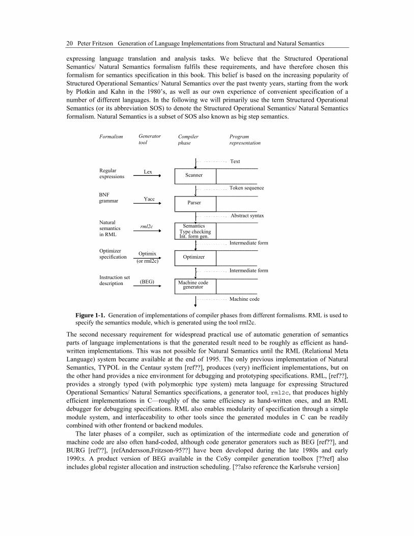
1.1 Compiler Generation The process of compiler generation is the automatic production of a compiler from formal specifications of source language, target language, and various intermediate formalisms and transformations. This is depicted in Figure 1-1, which also shows some examples of compiler generation tools and formalisms for the different phases of a typical compiler. Classical tools such as scanner generators (e.g. Lex) and parser generators (e.g. Yacc) were first developed in the 1970:s. Many similar generation tools for producing scanners and parsers exist.
However, the semantic analysis and intermediate code generation phase is still often hand-coded, although attribute grammar based tools have been available for practical usage for quite some time. Even though attribute grammars are easy to use for certain aspects of language specifications, they are less convenient when used for many other language aspects. Specifications tend to become long and involve many details and dependencies on external functions, rather than clearly expressing high level properties. Denotational Semantics is a formalism that provides more abstraction power, but is considered hard to use by most practitioners, and has problems with modularity of specifications and efficiency of produced implementations. We will not further discuss the matter of different specification formalisms, and refer the reader to other literature, e.g. [Pagan81??] which gives an easy to read introduction to several formalisms, including Attribute Grammars and Denotational Semantics. (??Also reference to [Louden2003??] and [Pierce2002??])
Semantic aspects of language translation include tasks such as type checking/type inference, symbol table handling, and generation of intermediate code. If automatic generation of translator modules for semantic tasks should become as common as generation of parsers from BNF grammars, we need a specification formalism that is both easy to use and that provides a high degree of abstraction power for
20 Peter Fritzson Generation of Language Implementations from Structural and Natural Semantics
expressing language translation and analysis tasks. We believe that the Structured Operational Semantics/ Natural Semantics formalism fulfils these requirements, and have therefore chosen this formalism for semantics specification in this book. This belief is based on the increasing popularity of Structured Operational Semantics/ Natural Semantics over the past twenty years, starting from the work by Plotkin and Kahn in the 1980’s, as well as our own experience of convenient specification of a number of different languages. In the following we will primarily use the term Structured Operational Semantics (or its abbreviation SOS) to denote the Structured Operational Semantics/ Natural Semantics formalism. Natural Semantics is a subset of SOS also known as big step semantics.
SemanticsType checkingInt. form gen.
Formalism Compiler Program Generator
Regular expressions
BNF grammar
Natural semantics
Optimizer specification
Instruction set description
Lex Scanner
Machine code generator
Yacc Parser
Text
Token sequence
Abstract syntax
Intermediate form
Intermediate form
Machine code
Optimizer
rml2c
Optimix
(BEG)
tool phase representation
(or rml2c)
in RML
Figure 1-1. Generation of implementations of compiler phases from different formalisms. RML is used to specify the semantics module, which is generated using the tool rml2c.
The second necessary requirement for widespread practical use of automatic generation of semantics parts of language implementations is that the generated result need to be roughly as efficient as hand-written implementations. This was not possible for Natural Semantics until the RML (Relational Meta Language) system became available at the end of 1995. The only previous implementation of Natural Semantics, TYPOL in the Centaur system [ref??], produces (very) inefficient implementations, but on the other hand provides a nice environment for debugging and prototyping specifications. RML, [ref??], provides a strongly typed (with polymorphic type system) meta language for expressing Structured Operational Semantics/ Natural Semantics specifications, a generator tool, rml2c, that produces highly efficient implementations in C—roughly of the same efficiency as hand-written ones, and an RML debugger for debugging specifications. RML also enables modularity of specification through a simple module system, and interfaceability to other tools since the generated modules in C can be readily combined with other frontend or backend modules.
The later phases of a compiler, such as optimization of the intermediate code and generation of machine code are also often hand-coded, although code generator generators such as BEG [ref??], and BURG [ref??], [refAndersson,Fritzson-95??] have been developed during the late 1980s and early 1990:s. A product version of BEG available in the CoSy compiler generation toolbox [??ref] also includes global register allocation and instruction scheduling. [??also reference the Karlsruhe version]

Chapter 1 Automatic Language Implementation 21
The optimization phase of compilers is generally hand coded, although some prototypes of optimizer generators have recently appeared. For example, an optimizer generator tool called Optimix [ref??], has appeared as one of the tools in the CoSy [ref??] compiler generation system.
RML can also be applied to portions of these other phases of compilers, such as optimization of intermediate code and final code generation. At this point, however, it is not clear how well Structured Operational Semantics and RML would work when applied to these tasks since we have not made any extensive application studies for optimization and final code generation. An informed guess is that intermediate code optimization would work well since this is usually a combination of analysis and transformation that can take advantage of patterns, transformation rules, and other features of RML.
Regarding final code generation modules, these are probably best produced by specialized tools such as BEG, which use specific algorithms such as dynamic programming for “optimal” instruction selection, and graph coloring for register allocation. However, the final answer is not yet known. In this book we only present a few very simple examples of final code generation, and essentially no examples of advanced code optimization.
1.2 Interpreter Generation The case of generating an interpreter from formal specifications can be regarded as a simplified special case of compiler generation. Although some systems interpret text directly (e.g command interpreters such as the Unix C shell), most systems first perform lexical and syntactic analysis to convert the program into some intermediate form, which is much more efficient to interpret than the textual representation. Type checking and other checking is usually done at run-time, either because this is required by the language definition (as for many interpreted languages such as LISP, Postscript, Smalltalk, etc.), or to minimize the delay until execution is started.
The semantic specification of a programming language intended as input for the generation of an interpreter if usually slightly different in style compared to a specification intended for compiler generation. Ideally, they would be exactly the same, and there exist techniques such as partial evaluation [ref??] that sometimes can produce compilers also from specifications of interpreters.
Interpreter /
Evaluator
Formalism Interpreter ProgramGenerator
Regularexpressions
BNF grammar
Natural semantics
Lex Scanner
Yacc Parser
Text
Token sequence
Abstract syntax
rml2c
tool phase representation
in RML
(Interpretive semantics)
Figure 1-2. Generation of a typical interpreter. The program text is converted into an abstract syntax representation, which is then evaluated by an interpreter generated by the RML system. Alternatively,

22 Peter Fritzson Generation of Language Implementations from Structural and Natural Semantics
some other intermediate representation such as postfix code can be produced, which is subsequently interpreted.
In practice, an interpretive style specification often expresses the meaning of a language construct by invoking a combination of well-defined primitives in the specification language. A compilation oriented specification, however, usually defines the meaning of language constructs by specifying a translation to an equivalent combination of well-defined constructs in some target language. In this text we will show examples of both interpretive and translation-oriented specifications.
(BRK)

23
Chapter 2 Expression Evaluators and Interpreters in RML
We will introduce the topic of language specification in Structured Operational Semantics/ Structured Operational Semantics using RML through a number of example languages.
The reader who would first prefer a general overview of some language properties of RML and its relation to Structured Operational Semantics may want to read Chapter 4 and Chapter 10 before continuing with these examples. On the other hand, the reader who has no previous experience with formal semantic specification and is more interested in “hands-on” use of RML for language implementation is recommended to continue directly with the current chapter and later take a quick glance at those chapters. We should also point out that Section ?? gives a short introduction to declarative programming with RML, whereas Chapter 4 (recommended) gives a more in-depth presentation of that topic.
First we present a very small expression language called Exp1.
2.1 The Exp1 Expression Language A very simple expression evaluator (interpreter) is our first example. This calculator evaluates constant expressions such as: 12 + 5*3
or -5 * (10 - 4)
The evaluator accepts text of a constant expression, which is converted to a sequence of tokens by the lexical analyzer (e.g. generated by Lex) and further to an abstract syntax tree by the parser (e.g. generated by Yacc). Finally the expression is evaluated by the interpreter (generated by the RML system), which in the above case would return the value 27. This corresponds to the general structure of a typical interpreter as depicted in Figure 1-2.
2.1.1 Concrete Syntax
The concrete syntax of the small expression language is shown below expressed as BNF rules in Yacc style, and lexical syntax of the allowed tokens as regular expressions in Lex style. All token names are in upper-case and start with T_ to be easily distinguishable from nonterminals which are in lower-case. /* Yacc BNF Syntax of the expression language Exp1 */ expression : term | expression weak_operator term term : u_element | term strong_operator u_element u_element : element | unary_operator element
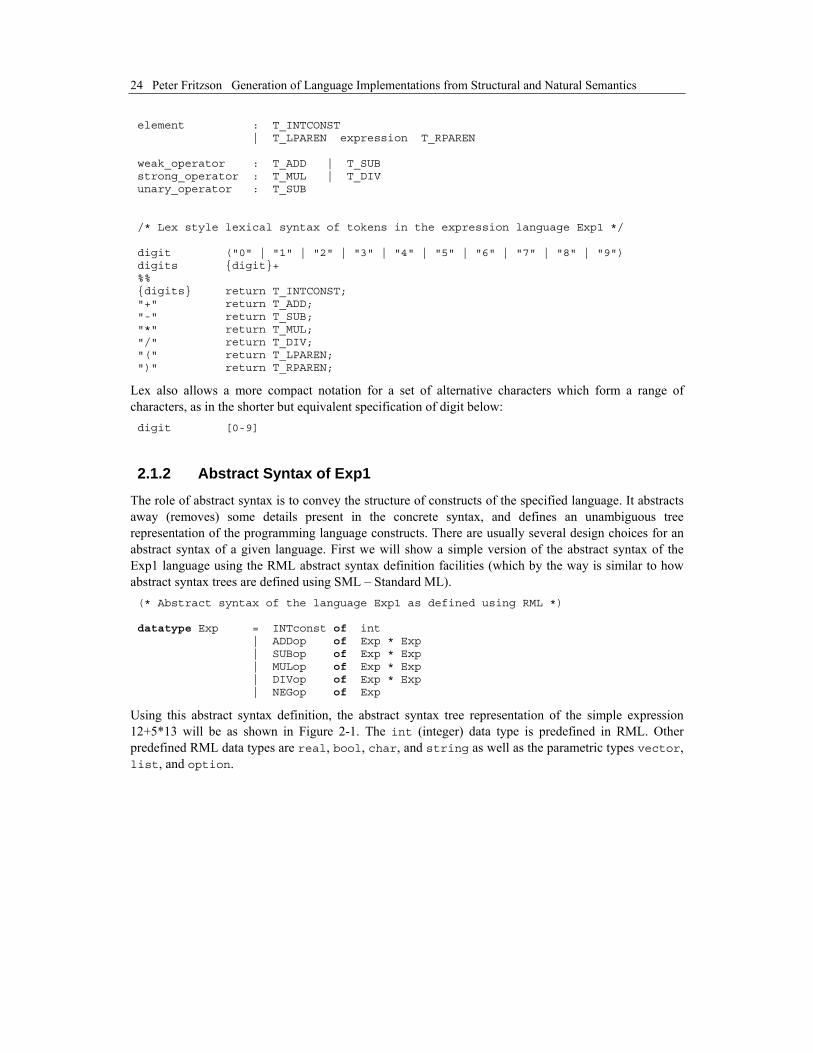
24 Peter Fritzson Generation of Language Implementations from Structural and Natural Semantics
element : T_INTCONST | T_LPAREN expression T_RPAREN weak_operator : T_ADD | T_SUB strong_operator : T_MUL | T_DIV unary_operator : T_SUB /* Lex style lexical syntax of tokens in the expression language Exp1 */ digit ("0" | "1" | "2" | "3" | "4" | "5" | "6" | "7" | "8" | "9") digits {digit}+ %% {digits} return T_INTCONST; "+" return T_ADD; "-" return T_SUB; "*" return T_MUL; "/" return T_DIV; "(" return T_LPAREN; ")" return T_RPAREN;
Lex also allows a more compact notation for a set of alternative characters which form a range of characters, as in the shorter but equivalent specification of digit below: digit [0-9]
2.1.2 Abstract Syntax of Exp1
The role of abstract syntax is to convey the structure of constructs of the specified language. It abstracts away (removes) some details present in the concrete syntax, and defines an unambiguous tree representation of the programming language constructs. There are usually several design choices for an abstract syntax of a given language. First we will show a simple version of the abstract syntax of the Exp1 language using the RML abstract syntax definition facilities (which by the way is similar to how abstract syntax trees are defined using SML – Standard ML). (* Abstract syntax of the language Exp1 as defined using RML *) datatype Exp = INTconst of int | ADDop of Exp * Exp | SUBop of Exp * Exp | MULop of Exp * Exp | DIVop of Exp * Exp | NEGop of Exp
Using this abstract syntax definition, the abstract syntax tree representation of the simple expression 12+5*13 will be as shown in Figure 2-1. The int (integer) data type is predefined in RML. Other predefined RML data types are real, bool, char, and string as well as the parametric types vector, list, and option.

Chapter 2 Expression Evaluators and Interpreters in RML 25
ADDop
MULop INTconst
12
INTconst
5
INTconst
13
Figure 2-1. Abstract syntax tree of 12+5*13 in the language Exp1.
The datatype declaration defines a union type Exp and constructors (here ADDop, MULop, INTconst) for each node type in the abstract syntax tree, as well as the types of the child nodes.
2.1.3 Semantics of Exp1
The semantics of the operations in the small expression language Exp1 follows below, expressed as a Structured Operational Semantics specification in RML. Such a specification typically consists of several relations, each of which contains one or more rules with the same name and formal parameters. In this simple example there is only one relation, here called eval, since we specify an expression evaluator. The relation is introduced by the keyword relation, followed by the name of the relation (here eval), a type signature telling input and output types (here Exp => int), an equality sign, a number of rules, and finally a keyword end. relation eval: Exp => int =
axiom eval( INTconst(ival) ) => ival (* eval of an integer node *) (* is the integer itself *)
(* Evaluation of an addition node ADDop is v3, if v3 is the result of * adding the evaluated results of its children e1 and e2 * Subtraction, multiplication, division operators have similar specs. *) rule eval(e1) => v1 & eval(e2) => v2 & int_add(v1,v2) => v3 ---------------------------------------------------------- eval( ADDop(e1,e2) ) => v3 rule eval(e1) => v1 & eval(e2) => v2 & int_sub(v1,v2) => v3 ---------------------------------------------------------- eval( SUBop(e1,e2) ) => v3 rule eval(e1) => v1 & eval(e2) => v2 & int_mul(v1,v2) => v3 ---------------------------------------------------------- eval( MULop(e1,e2) ) => v3 rule eval(e1) => v1 & eval(e2) => v2 & int_div(v1,v2) => v3 ---------------------------------------------------------- eval( DIVop(e1,e2) ) => v3 rule eval(e) => v1 & int_neg(v1) => v2 ----------------------------------- eval( NEGop(e) ) => v2 end
The general form of an RML rule is as follows:
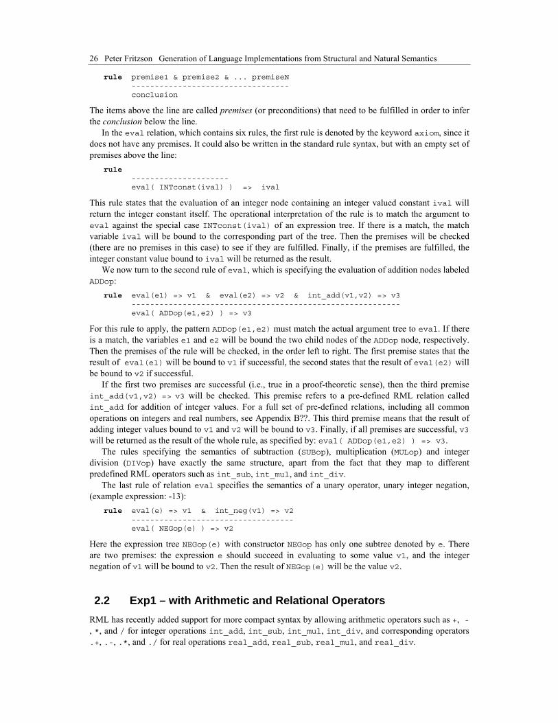
26 Peter Fritzson Generation of Language Implementations from Structural and Natural Semantics
rule premise1 & premise2 & ... premiseN ---------------------------------- conclusion
The items above the line are called premises (or preconditions) that need to be fulfilled in order to infer the conclusion below the line.
In the eval relation, which contains six rules, the first rule is denoted by the keyword axiom, since it does not have any premises. It could also be written in the standard rule syntax, but with an empty set of premises above the line: rule --------------------- eval( INTconst(ival) ) => ival
This rule states that the evaluation of an integer node containing an integer valued constant ival will return the integer constant itself. The operational interpretation of the rule is to match the argument to eval against the special case INTconst(ival) of an expression tree. If there is a match, the match variable ival will be bound to the corresponding part of the tree. Then the premises will be checked (there are no premises in this case) to see if they are fulfilled. Finally, if the premises are fulfilled, the integer constant value bound to ival will be returned as the result.
We now turn to the second rule of eval, which is specifying the evaluation of addition nodes labeled ADDop: rule eval(e1) => v1 & eval(e2) => v2 & int_add(v1,v2) => v3 ---------------------------------------------------------- eval( ADDop(e1,e2) ) => v3
For this rule to apply, the pattern ADDop(e1,e2) must match the actual argument tree to eval. If there is a match, the variables e1 and e2 will be bound the two child nodes of the ADDop node, respectively. Then the premises of the rule will be checked, in the order left to right. The first premise states that the result of eval(e1) will be bound to v1 if successful, the second states that the result of eval(e2) will be bound to v2 if successful.
If the first two premises are successful (i.e., true in a proof-theoretic sense), then the third premise int_add(v1,v2) => v3 will be checked. This premise refers to a pre-defined RML relation called int_add for addition of integer values. For a full set of pre-defined relations, including all common operations on integers and real numbers, see Appendix B??. This third premise means that the result of adding integer values bound to v1 and v2 will be bound to v3. Finally, if all premises are successful, v3 will be returned as the result of the whole rule, as specified by: eval( ADDop(e1,e2) ) => v3.
The rules specifying the semantics of subtraction (SUBop), multiplication (MULop) and integer division (DIVop) have exactly the same structure, apart from the fact that they map to different predefined RML operators such as int_sub, int_mul, and int_div.
The last rule of relation eval specifies the semantics of a unary operator, unary integer negation, (example expression: -13): rule eval(e) => v1 & int_neg(v1) => v2 ----------------------------------- eval( NEGop(e) ) => v2
Here the expression tree NEGop(e) with constructor NEGop has only one subtree denoted by e. There are two premises: the expression e should succeed in evaluating to some value v1, and the integer negation of v1 will be bound to v2. Then the result of NEGop(e) will be the value v2.
2.2 Exp1 – with Arithmetic and Relational Operators RML has recently added support for more compact syntax by allowing arithmetic operators such as +, -, *, and / for integer operations int_add, int_sub, int_mul, int_div, and corresponding operators .+, .-, .*, and ./ for real operations real_add, real_sub, real_mul, and real_div.
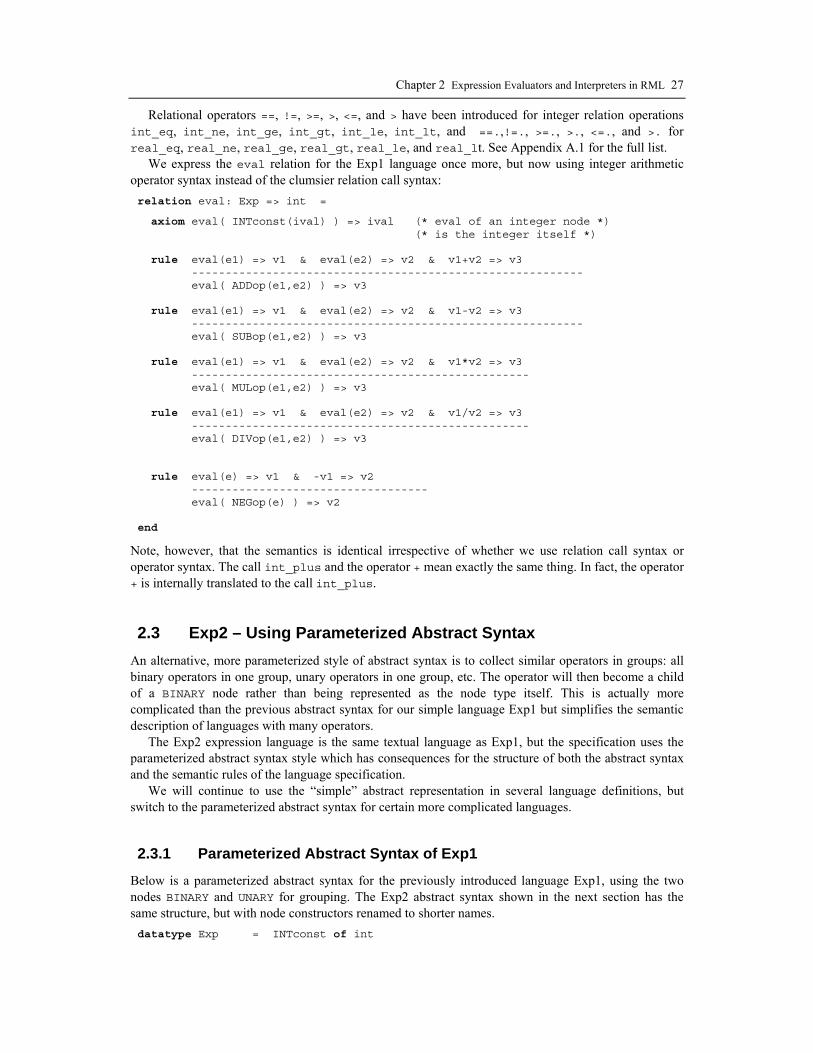
Chapter 2 Expression Evaluators and Interpreters in RML 27
Relational operators ==, !=, >=, >, <=, and > have been introduced for integer relation operations int_eq, int_ne, int_ge, int_gt, int_le, int_lt, and ==.,!=., >=., >., <=., and >. for real_eq, real_ne, real_ge, real_gt, real_le, and real_lt. See Appendix A.1 for the full list.
We express the eval relation for the Exp1 language once more, but now using integer arithmetic operator syntax instead of the clumsier relation call syntax: relation eval: Exp => int =
axiom eval( INTconst(ival) ) => ival (* eval of an integer node *) (* is the integer itself *)
rule eval(e1) => v1 & eval(e2) => v2 & v1+v2 => v3 ---------------------------------------------------------- eval( ADDop(e1,e2) ) => v3 rule eval(e1) => v1 & eval(e2) => v2 & v1-v2 => v3 ---------------------------------------------------------- eval( SUBop(e1,e2) ) => v3 rule eval(e1) => v1 & eval(e2) => v2 & v1*v2 => v3 -------------------------------------------------- eval( MULop(e1,e2) ) => v3 rule eval(e1) => v1 & eval(e2) => v2 & v1/v2 => v3 -------------------------------------------------- eval( DIVop(e1,e2) ) => v3 rule eval(e) => v1 & -v1 => v2 ----------------------------------- eval( NEGop(e) ) => v2 end
Note, however, that the semantics is identical irrespective of whether we use relation call syntax or operator syntax. The call int_plus and the operator + mean exactly the same thing. In fact, the operator + is internally translated to the call int_plus.
2.3 Exp2 – Using Parameterized Abstract Syntax An alternative, more parameterized style of abstract syntax is to collect similar operators in groups: all binary operators in one group, unary operators in one group, etc. The operator will then become a child of a BINARY node rather than being represented as the node type itself. This is actually more complicated than the previous abstract syntax for our simple language Exp1 but simplifies the semantic description of languages with many operators.
The Exp2 expression language is the same textual language as Exp1, but the specification uses the parameterized abstract syntax style which has consequences for the structure of both the abstract syntax and the semantic rules of the language specification.
We will continue to use the “simple” abstract representation in several language definitions, but switch to the parameterized abstract syntax for certain more complicated languages.
2.3.1 Parameterized Abstract Syntax of Exp1
Below is a parameterized abstract syntax for the previously introduced language Exp1, using the two nodes BINARY and UNARY for grouping. The Exp2 abstract syntax shown in the next section has the same structure, but with node constructors renamed to shorter names. datatype Exp = INTconst of int

28 Peter Fritzson Generation of Language Implementations from Structural and Natural Semantics
| BINARY of Exp * BinOp * Exp | UNARY of UnOp * Exp datatype BinOp = ADDop | SUBop | MULop | DIVop datatype UnOp = NEGop
BINARY
BINARYINTconst
12
INTconst
5
INTconst
13
ADDop
MULop
Figure 2-2. A parameterized abstract syntax tree of 12+5*13 in the language Exp1. Compare to the abstract syntax tree in Figure 2-1.
2.3.2 Parameterized Abstract Syntax of Exp2
Here follows the abstract syntax of the Exp2 language. The two node constructors BINARY and UNARY have been introduced to represent any binary or unary operator, respectively. Constructor names have been shortened to INT, ADD, SUB, MUL, DIV and NEG. datatype Exp = INT of int | BINARY of Exp * BinOp * Exp | UNARY of UnOp * Exp datatype BinOp = ADD | SUB | MUL | DIV datatype UnOp = NEG
2.3.3 Semantics of Exp2
Here follows the semantic rules for the expression language Exp2. As already mentioned, constructor names have been shortened compared to the specification of Exp1. Two rules have been introduced for constructors BINARY and UNARY, which capture the common characteristics of all binary and unary operators, respectively. Two new relations apply_binop and apply_unop have been introduced, which describe the special properties of each binary and unary operator, respectively. relation eval: Exp => int =
Evaluation of an INT node gives the integer constant value itself: axiom eval( INT(ival) ) => ival
Evaluation of a binary operator node BINARY gives v3, if v3 is the result of applying the binary operator to v1 and v2, which are the evaluated results of its children e1 and e2: rule eval(e1) => v1 & eval(e2) => v2 & apply_binop(binop,v1,v2) => v3 --------------------------------- eval( BINARY(e1,binop,e2) ) => v3
Evaluation of a unary operator node UNARY gives v2, if its child e can be evaluated to a value v1, and the unary operator can be successfully applied to value v1, giving the result value v2.

Chapter 2 Expression Evaluators and Interpreters in RML 29
rule eval(e) => v1 & apply_unop(unop,v1) => v2 -------------------------------------------- eval( UNARY(unop,e) ) => v2 end (* of eval *)
The relation apply_binop accepts a binary operator and two integer values. If the operator successfully can be applied to these values the integer result will be returned. relation apply_binop: (BinOp,int,int) => int = rule int_add(v1,v2) => v3 ---------------------- apply_binop(ADD,v1,v2) => v3 rule int_sub(v1,v2) => v3 ---------------------- apply_binop(SUB,v1,v2) => v3 rule int_mul(v1,v2) => v3 ---------------------- apply_binop(MUL,v1,v2) => v3 rule int_div(v1,v2) => v3 ----------------------- apply_binop(DIV,v1,v2) => v3 end (* of apply_binop *)
The relation apply_unop accepts a unary operator and an integer value. If the operator successfully can be applied to this value an integer result will be returned. relation apply_unop: (UnOp,int) => int =
rule int_neg(v) => v2 ----------------------- apply_unop(NEG,v) => v2 end (* of apply_unop *)
For the small language Exp2 the semantic description has become more complicated since we now need three relations, eval, apply_binop and apply_unop, instead of just eval. In the following, we will use the simple abstract syntax style for small specifications. The parameterized abstract syntax style will only be used for larger specifications where it actually helps in structuring and simplifying the specification.
2.4 Using the RML Specification Language Before continuing the series of language specifications in Structured Operational Semantics expressed in RML, it is will be useful to say a few words about the RML language itself, its relation to the Structured Operational Semantics formalism, and its usage style. A more in-depth treatment of these topics can be found in Chapter 4.
2.4.1 Structured Operational Semantics/ Natural Semantics and RML
We have already seen several examples of relations containing one or more rules, as expressed in RML syntax. A rather general schema for the structure of an RML relation, here denoted ThisRelation, is shown below: relation ThisRelation

30 Peter Fritzson Generation of Language Implementations from Structural and Natural Semantics
rule RelationX(H1,T1) => R1 & RelationY(H2,T2,TX2) => R2 & ... RelationX(Hn,Tn) => Rn & ... <condition> ----------------------------- ThisRelation(H,T) => R ... end
We note that several relations are called in the premises above the line in the above rule. RelationX is a ternary relation since it relates three quantities: two inputs (H1,T1) and one output: R1. RelationY is a quadruple relation, with three inputs (H2,T2,TX2) and one output: R2. The result of the whole relation ThisRelation is denoted by R in the above schematic example.
In the traditional style of a Structured Operational Semantics syntax, used in many books and papers, Structured Operational Semantics rules are expressed in a similar rule syntax, with the difference that relations are usually denoted by (sometimes cryptic) operators instead of alphanumeric names, and variable names are usually short—one or two letters at most.
For example, RelationX can be represented by a ternary operator such as (arg1 |– arg2 : arg3) relating three arguments by using the two operator symbols |– and :, and RelationY can be represented by a quadruple operator such as (arg1 |– arg2 , arg3 : arg4) using the three operator symbols |–, comma, and colon.
As a comparison—a common example of a ternary operator in programming languages is if-expressions, e.g. in Modelica syntax: (if arg1 then arg2 else arg3), and in C language syntax: (arg1 ? arg2 : arg3).
The above schematic rule can be expressed as follows using the traditional Structured Operational Semantics style:
H1 |– T1 : R1 , H2 |– T2 , TX2 : R2 . . . Hn |– Tn : Rn ————————————————————— if <condition> H |– T : R
The used Structured Operational Semantics notation can be briefly explained as follows:
• Hi are hypotheses. • Ti, TXi, etc., are terms in general. • Ri are results. • <condition> is an optional side condition.
The rule may be interpreted as follows: in order to prove a conclusion such as H |– T : R, one must first prove all premises above the line H1 |– T1 : R1 , . . . Hn |– Tn : Rn. The side condition <condition>, if present, must also be satisfied. Items such as the premises and the conclusion, e.g. Hi |– Ti : Ri, are also known as sequents or propositions.
2.4.2 Short Introduction to Declarative Programming in RML
We have already stated that RML is a declarative specification language for writing programming language specifications in Structured Operational Semantics style. Since RML is declarative, it can also be viewed as a kind of functional programming language. An RML relation maps inputs to outputs, just as a function, but also has two additional properties not found in functions:
• Relations can succeed or fail. • Local backtracking between rules in a relation can occur.

Chapter 2 Expression Evaluators and Interpreters in RML 31
The fac example below shows a relation calculating factorials. This is an example of not using RML for language specification, but to state a small declarative (i.e., functional) program: relation fac: int => int =
rule ----------- fac(0) => 1 rule int_gt(n, 0) => true & int_sub(n, 1) => n2 & fac(n2) => res2 & int_mult(n, res2) => result --------------------------- fac(n) => result end
The first line specifies the name (fac) and type signature (int => int) of the relation. In this example an integer factorial function is computed, which means that both the input parameter and the result are of type int (integer).
Next comes the rules, which make up the body of the relation. The first rule in the above example can be interpreted as follows:
• If the relation is called to compute the factorial of the value 0 (i.e. matching the “pattern” fac(0)), then the result is the value 1.
This corresponds to the base case of a recursive function calculating factorials. The rule can alternatively be stated using the equivalent but shorter RML axiom syntax since this rule has no premises: axiom fac(0) => 1
The first rule will be invoked if the argument matches the pattern fac(0) of the rule. If this is not the case, the next rule will be tried, if this rule does not match, the next one will be tried, and so on. If no rule matches the arguments, the call to the relation will fail.
The second rule of the fac relation handles the general case of a factorial function computation when the input value n is greater than zero, i.e., int_gt(n, 0) => true. It can be interpreted as follows:
• If the factorial is to be computed on a value n, i.e., fac(n), and n>0, then compute n-1 and call the result n2, compute fac(n2) which is called res2, and finally multiply res2 by n, to be returned as the result, i.e., n*f(n-1), of the rule.
Thus in order to prove the conclusion of a rule, the different premises above the line in the rule are tried in a top-to-bottom / left-to-right order. The called relations int_gt, int_sub, and int_mult are builtin RML primitive relations for the integer operations “greater than”, “subtraction”, and “multiplication” respectively.
2.4.2.1 Handling Failure
If the fac relation is used to compute the factorial of a negative value an important property of RML is shown, since the fac relation will in this case fail.
A factorial call with a negative argument does not match the first rule, since all negative values differs from zero. Neither can the second rule be applied, since the premise int_gt(n,0) is not fulfilled for negative values of n.
Thus the relation will fail, meaning it will not return an ordinary value to the calling relation. After a fail has occurred in a rule or in some relation called from that rule, backtracking takes place, and the next rule in the current relation is tried instead.
However, relations with built-in failure handling can be useful, as in the following example: relation fac_failsafe: int => () =
rule fac(n) => result & int_string(result) => string_result &

32 Peter Fritzson Generation of Language Implementations from Structural and Natural Semantics
print "Res: " & print string_result & print "\n" ------------- fac_failsafe(n) rule not fac(n) => _ & print "Cannot apply factorial relation " & print "to n.\n" --------------- fac_failsafe(n)
The first rule handles the case when the fac relation computes the value and returns successfully. In this case the value is converted to a string and printed using the built-in RML print relation.
The second rule is tried if the first rule fails, for example if the relation fac_failsafe is called with a negative argument, e.g. fac(-1).
In the second rule a new keyword, not, is introduced in the expression not fac(n) which succeeds if the call fac(n) fails. Then an error message is printed by the second rule.
It is important to note that fail is quite different from the logical value false. A relation returning false would still succeed since it returns a value. The builtin relation bool_not operates on the logical values true and false, and is quite different from the not operator. See also Section 4.5.2.
2.5 The Assignments Language – Introducing Environments The Assignments language extends our simple evaluator with variables. For example, the assignment: a := 5 + 3*10
will store the value of the evaluated expression (here 35) into the variable a. The value of this variable can later be looked up and used for computing other expressions: b := 100 + a
d := 10 * b
giving the values 135 and 1350 for b and d, respectively. Expressions may also contain embedded assignments as in the example below: e := 50 + (d := a + 100)
2.5.1 Environments
To handle variables, we need a mechanism for associating values with identifiers. This mapping from identifiers to values is called environment, and can be represented as a set of pairs (identifier,value). A function called lookup is introduced for looking up the associated value for a given identifier. An association of some value or other structure to an identifier is called a binding. An identifier is bound to a value within some environment.
There are several possible choices of data structures for representing environments. The simplest representation, often used in formal specifications, is to use a linked list of (identifier,value) pairs. This has the advantage of simplicity, but gives long lookup times due to linear search if there are many identifiers in the list. Other, more complicated, choices are binary trees (see Section 4.10) or hash tables. Such representations are commonly used to provide fast lookup in product quality compilers or interpreters.
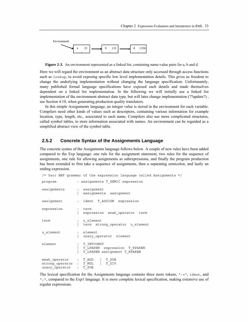
Chapter 2 Expression Evaluators and Interpreters in RML 33
a 35 b 135 d 1350
Environment
Figure 2-3. An environment represented as a linked list, containing name-value pairs for a, b and d.
Here we will regard the environment as an abstract data structure only accessed through access functions such as lookup, to avoid exposing specific low level implementation details. This gives us freedom to change the underlying implementation without changing the language specification. Unfortunately, many published formal language specifications have exposed such details and made themselves dependent on a linked list implementation. In the following we will initially use a linked list implementation of the environment abstract data type, but will later change implementation (??update?) , see Section 4.10, when generating production quality translators.
In this simple Assignments language, an integer value is stored in the environment for each variable. Compilers need other kinds of values such as descriptors, containing various information for example location, type, length, etc., associated to each name. Compilers also use more complicated structures, called symbol tables, to store information associated with names. An environment can be regarded as a simplified abstract view of the symbol table.
2.5.2 Concrete Syntax of the Assignments Language
The concrete syntax of the Assignments language follows below. A couple of new rules have been added compared to the Exp language: one rule for the assignment statement, two rules for the sequence of assignments, one rule for allowing assignments as subexpressions, and finally the program production has been extended to first take a sequence of assignments, then a separating semicolon, and lastly an ending expression. /* Yacc BNF grammar of the expression language called Assignments */
program : assignments T_SEMIC expression assignments : assignment | assignments assignment assignment : ident T_ASSIGN expression expression : term | expression weak_operator term term : u_element | term strong_operator u_element u_element : element | unary_operator element element : T_INTCONST | T_LPAREN expression T_RPAREN | T_LPAREN assignment T_RPAREN weak_operator : T_ADD | T_SUB strong_operator : T_MUL | T_DIV unary_operator : T_SUB
The lexical specification for the Assignments language contains three more tokens, ":=", ident, and ";", compared to the Exp1 language. It is more complete lexical specification, making extensive use of regular expressions.

34 Peter Fritzson Generation of Language Implementations from Structural and Natural Semantics
Whitespace represents one or more blanks, tabs or new lines, and is ignored, i.e., no token is returned. A letter is a letter a-z or A-Z or underscore. An identifier (ident) is a letter followed by zero or more letters or digits. A digit is a character within the range 0-9. Digits is one or more of digit. An integer constant (intcon) is the same as digits. The function lex_ident returns the token T_IDENT and converts the scanned name to an atom representation stored in the global variable yylval.voidp which is used by the parser to obtain the identifier. The function lex_icon returns the token T_INTCONST and stores the integer constant converted into binary form in the same yyval.voidp. /* Lex style lexical syntax of tokens in the language Assignments */ whitespace [ \t\n]+ letter [a-zA-Z_] ident {letter} ({letter} | {digit})* digit [0-9] digits {digit}+ %% {whitespace} ; {ident} return lex_ident(); /* T_IDENT */ {digits} return lex_icon(); /* T_INTCONST */ ":=" return T_ASSIGN; "+" return T_ADD; "-" return T_SUB; "*" return T_MUL; "/" return T_DIV; "(" return T_LPAREN; ")" return T_RPAREN; ";" return T_SEMIC;
2.5.3 Abstract Syntax of the Assignments Language
We introduce a few additional node types compared to the Exp1 language: the ASSIGN constructor representing assignment and the IDENT constructor for identifiers. datatype Exp = IDENT of Ident | ASSIGN of Ident * Exp
Now we have also added a new abstract syntax type Program that represents an entire program as a list of assignments followed by an expression: datatype Program = PROGRAM of Exp list * Exp
The first list of expressions contains the initial list of assignments made before the ending expression will be evaluated.
The new type Ident is exactly the same as the builtin RML type string (but in some later language specifications we might use the more efficient atom representation of identifier names). The RML type declaration just introduces new names for existing types. The type Value is the same as int and represents integer values. type Ident = string type Value = int
The environment type Env is represented as a list of pairs of (identifier,value) representing bindings of type VarBnd of identifiers to values. The RML syntax for tuples is: (item1, item2, ... itemN) of which a pair is a special case with two items. The tuple type syntax is itemtype1 * itemtype2 *... itemtypeN. The RML list keyword denotes a list type. type VarBnd = Ident * int type Env = VarBnd list
Below follows all abstract syntax declarations needed for the specification of the Assignments language. (* Abstract syntax for the Assignments language *)

Chapter 2 Expression Evaluators and Interpreters in RML 35
datatype Program = PROGRAM of Exp list * Exp type Ident = string datatype Exp = INT of int | IDENT of Ident | BINARY of Exp * BinOp * Exp | UNARY of UnOp* Exp | ASSIGN of Ident * Exp datatype BinOp = ADD | SUB | MUL | DIV datatype UnOp = NEG (* Values stored in environments *) type Value = int (* Bindings and environments *) type VarBnd = (Ident * Value) type Env = VarBnd list
2.5.4 Semantics of the Assignments Language
As previously mentioned, the Assignments language introduces the treatment of variables and the assignment statement to the former Exp2 language. Adding variables means that we need to remember their values between one expression and the next. This is handled by an environment (also known as evaluation context), which in our case is represented as list of variable-value pairs.
A semantic rule will evaluate each descendent expression in one environment, modify the environment if necessary, and then pass the value of the expression and the new environment to the next evaluation.
2.5.4.1 Semantics of Lookup in Environments
To check whether an identifier is already present in an environment, and if so, return its value, we introduce the relation (largely a function) lookup, see also Section 4.10. If there is no value associated with the identifier, lookup will fail. relation lookup: (Env,Ident) => Value = ...
This version of lookup performs a linear search of an environment represented as a list of pairs (identifier,value). The first rule, shown below, deals with the case when the identifier is present in the leftmost (most recent) pair in the environment.
It will try to match the (id2,value) :: _ pattern against the environment argument. The :: is the cons operator for adding a new element at the front of a list; the underscore _ is a “wildcard” pattern that matches anything. If there is a match, id2 will become bound to the identifier of that pair, and value will be bound to its associated value. If the premise id = id2 is fulfilled, then value will be returned as the result of lookup, otherwise the next rule will be applied. rule id = id2 ------------------------------ lookup((id2,value) :: _, id) => value
For example, the environment list (env) depicted in Figure 2-3 shown is below: [(a,35), (b,135), (d,1350)]
It is the result of several cons operations: (a,35) :: (b,135) :: (d,1350) :: nil
An example lookup call: lookup(env, a)

36 Peter Fritzson Generation of Language Implementations from Structural and Natural Semantics
will match the pattern lookup((id2,value) :: _, id)
of the first rule, and thereby bind id2 to a, value to 35, and id to a. Since the premise id=id2 is fulfilled, the value 35 will be returned.
The second rule of lookup deals with the case when the identifier might be present in the rest of the list (i.e., not in the leftmost pair). The pattern (id2,_) :: rest binds id2 to the identifier in the leftmost pair, and rest to the rest of the list.
For a call such as lookup(env, b), id2 will be bound to a, rest to [(b,135),(d,1350)], and id to b.
The first premise of the rule below states that id is not in the leftmost pair ((a,35) in the above example call), whereas the second premise retrieves the value from the rest of the environment if it succeeds. rule not id=id2 & lookup(rest, id) => value ------------------------------ lookup((id2,_) :: rest, id) => value
The whole lookup relation follows below: relation lookup: (Env,Ident) => Value = (* lookup returns the value associated with an identifier. * If no association is present, lookup will fail. *) (* Identifier id is found in the first pair of the list, and value * is returned. *) rule id = id2 ------------------------------ lookup((id2,value) :: _, id) => value (* id is not found in the first pair of the list, and lookup will * recursively search the rest of the list. If found, value is returned. *) rule not id=id2 & lookup(rest, id) => value ------------------------------------- lookup((id2,_) :: rest, id) => value end
We have two following rules for the occurrence of an identifier (i.e., a variable) in an expression:
• If the variable is not yet in the environment, initialize it to zero and return its zero value and the new environment containing the added variable.
• If the variable is already in the environment, return its value together with the environment.
This is expressed by the relation lookupextend below: relation lookupextend: (Env,Ident) => (Env,Value) =
rule not lookup(env,id) => v & (id,0) :: env => env2 ----------------------------- lookupextend(env, id) => (env2,0) rule lookup(env,id) => value -------------------------------- lookupextend(env, id) => (env,value) end
For example, the following call on the above example environment env: lookupextend(env,x)
will return the following environment together with the value 0:
Chapter 2 Expression Evaluators and Interpreters in RML 37
[(x,0), (a,35), (b,135), (d,1350)]
For the evaluation of an assignment (node ASSIGN) we need to store the variable and its value in an updated environment, expressed by the following two rules:
• If the variable on the left hand side of the assignment is not yet in the environment, associate it with the value obtained from evaluating the expression on the right hand side, store this in the environment, and return the new value and the updated environment.
• If the variable on the left hand side is already in the environment, replace the current variable value with the value from the right hand side, and return the new value and the updated environment.
We actually cheat a bit in the relation update below. Both lookupextend and update add a new pair (id,value) at the front of the environment represented as a list, even if the variable is already present. Since lookup will always search the environment association list from beginning to end, it will always return the most recent value, which gives the same semantics in terms of computational behavior but consumes more storage than a solution which would locate the existing pair and replace the value. relation update: (Env,Ident,Value) => Env = axiom update(env,id,value) => ((id,value) :: env) end
For example, the following call to update the variable x in the above example environment env: update(env,x,999)
will give the following environment list: [(x,999), (a,35), (b,135), (d,1350)]
One more call update(env,x,988) on the returned environment will give: [(x,988), (x,999), (a,35), (b,135), (d,1350)]
A call to lookup x in the new environment (here called env3): lookup(env3, x)
will return the most recent value of x, which is 988.
2.5.4.2 Evaluation Semantics
The eval relation from the earlier Exp2 language has been extended with rules for assignment (ASSIGN) and variables (IDENT), as well as accepting an environment as an extra argument and returning an (updated) environment as a result. In the rule to evaluate an IDENT node, lookupextend returns a possibly updated environment env2 and the value associated with identifier id in the current environment env. If there is no such value, identifier id will be bound to zero and the current environment will be updated to become env2. relation eval: (Env,Exp) => (Env,int) = (* eval of an integer constant node in an environment is the integer * value together with the unchanged environment. *) axiom eval(env,INT(ival) ) => (env,ival) (* eval of an identifier node will lookup the identifier and return a * value if present; otherwise insert a binding to zero, and return zero. *) rule lookupextend(env,id) => (env2,value) ----------------------------------- eval(env,IDENT(id)) => (env2,value) (* eval of an assignment node returns the updated environment and

38 Peter Fritzson Generation of Language Implementations from Structural and Natural Semantics
* the assigned value. *) rule eval(env,exp) => (env2,value) & update(env2,id,value) => env3 ---------------------------------------- eval(env,ASSIGN(id,exp)) => (env3,value)
The rules below specify the evaluation of the binary (ADD, SUB, MUL, DIV) and unary (NEG) operators. The first rule specifies that the evaluation of an binary node BINARY(e1,binop,e2) in an environment env1 is a possibly changed environment env3 and a value v3, provided that relation eval succeeds in evaluating e1 to the value v2 and possibly a new environment env2, and e2 successfully evaluates e2 to the value v2 and possibly a new environment env3. Finally, the apply_binop relation is used apply the operator to the two evaluated values. The reason for returning new environments is that expressions may contain embedded assignments, for example: e := 35 + (d := a + 100). The rule for unary operators is similar. (* eval of a binary node BINARY(e1,binop,e2), etc. in an environment env *) rule eval(env1, e1) => (env2, v1) & eval(env2, e2) => (env3, v2) & apply_binop(binop,v1,v2) => v3 --------------------------------- eval(env1, BINARY(e1,binop,e2) ) => (env3, v3) rule eval(env1, e) => (env2, v1) & apply_unop(unop,v1) => v2 -------------------------------------------- eval(env1, UNARY(unop,e) ) => (env2, v2)
In Section 2.7 the Assignments language will be extended into a language called AssignTwoType, that can handle expressions containing constants and variables of two types: real and integer, which has interesting consequences for the semantics of the evaluation rules and storing values in the environment.
2.6 PAM – Introducing Control Structures and I/O PAM is a Pascal-like language that is too small to be useful for serious programming, but big enough to illustrate several important features of programming languages such as control structures, including loops (but excluding goto), and simple input/output. However, it does not include procedures and several types. Only integer variables and values are dealt with during computation, although boolean values can occur temporarily in comparisons for if- or while-statements.
The language was originally presented by Frank Pagan in his book Formal Specification of Programming Languages [ref??], which gives a very pedagogical introduction to formal specification using several formalisms such as attribute grammars, two-level grammars, operational semantics, denotational semantics and axiomatic semantics. The reader who would like a more in-depth description of PAM and would like to learn about other formalisms than Structured Operational Semantics is highly recommended to read Pagan’s book. We deliberately chose to include a specification of the same PAM language in this text, to allow the reader to make direct comparisons between a Structured Operational Semantics specification and corresponding specifications in other formalisms by studying Pagan’s book in parallel.
2.6.1 Examples of PAM Programs
A PAM program consists of a series of statements, as in the example below where the factorial of a number N is computed. First the number N is read from the input stream. Then the special case of
Chapter 2 Expression Evaluators and Interpreters in RML 39
factorial of zero is dealt with, giving the value 1. Note that factorial of a negative number is not handled by this program, not even by an error message since there are no strings in this language.
The factorial for N>0 is computed by the else-part of the if-statement, which contains a definite loop:
to expression do series-of-statement end
This loop computes series-of-statement a definite number of times given by first evaluating expression. In the example below, to N do ... end will compute the factorial by iterating N times. Alternatively, we could have expressed this as an indefinite loop, i.e., a while statement:
while comparison do series-of-statement end
which will evaluate series-of-statement as long as comparison is true. (* Computing factorial of the number N, and store in variable Fak *) (* N is read from the input stream; Fak is written to the output *) (* Fak is 1 * 2 * .... (N-1) * N *) read N; if N=0 then Fak := 1; else if N>0 then Fak := 1; I := 0; to N do I := I+1; Fak := Fak*I; end endif endif write Fak;
Variables are not declared in this language, they are created when they are assigned values. The usual arithmetic operators “+”, “-” with weak precedence and “*”, “/” with stronger precedence, are included. Comparisons are expressed by the relational operators “<”, “<=”, “=”, “>=”, “>”. One small change has been done to PAM as compared to Pagan’s book: the reserved word FI has been replaced by the more readable endif.
2.6.2 Concrete Syntax of PAM
The concrete syntax of the PAM language is given as a BNF grammar below. A program is a series of statement. A statement is an input statement (read id1,id2,...); an output statement (write id1,id2...); an assignment statement (id := expression); an if-then conditional statement (if expression then series-of-statement endif), an if-then-else conditional statement (if expression then series-of-statement else series-of-statement endif), a definite loop for a fixed number of iterations (to expression do series-of-statement end), or a while-loop for an indefinite number of iterations (while comparison do series-of-statement end). The usual arithmetic expressions are included, as well as comparisons using relational operators. /* Yacc BNF grammar of the PAM language */ program : series series : statement | statements series statement : input_statement T_SEMIC | output_statement T_SEMIC | assignment_statement T_SEMIC | conditional_statement | definite_loop

40 Peter Fritzson Generation of Language Implementations from Structural and Natural Semantics
| while_loop input_statement : T_READ variable_list output_statement : T_WRITE variable_list variable_list : variable | variable variable_list assignment_statement : variable T_ASSIGN expression conditional_statement : T_IF comparison T_THEN series T_ENDIF | T_IF comparison T_THEN series T_ELSE series T_ENDIF definite_loop | T_TO expression T_DO series T_END while_loop | T_WHILE comparison T_DO series T_END expression : term | expression weak_operator term term : element | term strong_operator element element : constant | variable | T_LPAREN expression T_RPAREN comparison : expression relation expression variable : T_IDENT constant : T_INTCONST relation : T_EQ | T_LE | T_LT T_GT | T_GE | T_NE weak_operator : T_ADD | T_SUB strong_operator : T_MUL | T_DIV
The lexical syntax of the PAM language has two extensions compared to the previously presented Assignments language: tokens for relational operators “<”, “<=”, “=”, “<>”, “>=”, “>” and tokens for reserved words: if, then, else ,endif, while, do, end, to, read, write. The function lex_ident checks if a possible identifier is a reserved word, and in that case returns one of the tokens T_IF, T_THEN, T_ELSE, T_ENDIF, T_ELSE, T_WHILE, T_DO, T_END, T_TO, T_READ or T_WRITE. /* Lex style lexical syntax of tokens in the PAM language */ whitespace [ \t\n]+ letter [a-zA-Z] ident {letter} ({letter} | {digit})* digit [0-9] digits {digit}+ icon {digits} %% {whitespace} ; {ident} return lex_ident(); /* T_IDENT or reserved word tokens */ /* Reserved words: if,then,else,endif,while,do,end,to,read,write */ {digits} return lex_icon(); /* T_INTCONST */ ":=" return T_ASSIGN; "+" return T_ADD; "-" return T_SUB; "*" return T_MUL; "/" return T_DIV; "(" return T_LPAREN; ")" return T_RPAREN;

Chapter 2 Expression Evaluators and Interpreters in RML 41
"<" return T_LT; "<=" return T_LE; "=" return T_EQ; "<>" return T_NE; ">=" return T_GE; ">" return T_GT;
2.6.3 Abstract Syntax of PAM
Since PAM is slightly more complicated than previous languages we choose the parameterized style of abstract syntax, first introduced in Section 2.3 and Section 2.3. This style is better at grouping related semantic constructs and thus making the semantic specification more concise and better structured.
In comparison to the Assignments language, we have introduced relational operators (RelOp) and the RELATION constructor which belongs to the set of expression nodes (Exp). There is also a union type Stmt for different kinds of statements. Note that statements are different from expressions in that they do not return a value but update the value environment and/or modify the input or output stream. The constructor SEQ allows the representation of statement sequences, whereas SKIP represents the empty statement. (* Parameterized abstract syntax for the PAM language *) type Ident = string datatype BinOp = ADD | SUB | MUL | DIV datatype RelOp = EQ | GT | LT | LE | GE | NE datatype Exp = INT of int | IDENT of Ident | BINARY of Exp * BinOp * Exp | RELATION of Exp * RelOp * Exp datatype Stmt = ASSIGN of Ident * Exp (* Id := Exp *) | IF of Exp * Stmt * Stmt (* if Exp then Stmt..*) | WHILE of Exp * Stmt (* while Exp do Stmt*) | TODO of Exp * Stmt (* to Exp do Stmt...*) | READ of Ident list (* read id1,id2,...*) | WRITE of Ident list (* write id1,id2,..*) | SEQ of Stmt * Stmt (* Stmt1; Stmt2 *) | SKIP (* ; empty stmt *)
The type specifications below are not part of the abstract syntax of the language constructs, but needed to model the static and dynamic semantics of PAM. As for the Assignments language, the environment (Env) is a mapping from identifiers to values, used to store and retrieve variable values. Here it is represented as a list of pairs of variable bindings (VarBnd).
We also introduce a data type Value for values obtained during expression evaluation. Even though only integer values tagged by the constructor INTval are stored in the environment, boolean values, represented by BOOLval(bool), occur when evaluation comparison relations.
Since PAM contains input and output statements, we need to model the overall state including both variable bindings and input and output files. This could have been done (as in Pascal [ref **]) by introducing two predefined variables in the environment denoting the standard input stream and output stream, respectively. Since standard input/output streams are not part of the PAM language definition we choose another solution. The concept of state is introduced, of type State, which is represented as a triple of environment, input stream and output stream (Env,Stream,Stream). The term configuration is sometimes used for this kind of state. (* Types needed for modeling static and dynamic semantics *) (* Variable binding and environment type *) type VarBnd = Ident * Value type Env = VarBnd list

42 Peter Fritzson Generation of Language Implementations from Structural and Natural Semantics
(* Value type needed for evaluation *) datatype Value = INTval of int | BOOLval of bool abstype OutStream = ?? (**? should be a builtin RML type for read/write? *) abstype InStream = ?? (**? should be a builtin RML type for read/write? *) (* State type, containing Env, input Stream and output Stream *) type State = (Env,InStream,OutStream) module Out: abstype Stream; Int: (Stream,Int) => Stream String: ?? end module In: abstype Stream; Int: Stream => (Stream,Int) (** scanf %d) String: Stream => (Stream,String) (** antal char argu Char: Stream => (Stream,Char) (** antal char argu Real: Stream => (Stream,Real) end (**?? Se t.ex. parse för Petrol och mini-ML) (** Fungerar endast om det ej sker backtracking som påverkar sekvensen av I/O operationer, t.ex. om någonting kan faila.) T.ex. om flera regler kan matcha, och en regel utför en sidoeffekt; Exempel: en interpretator med funktionsanrop i predikat till if-sats; detta funktionsanrop ger fail. Dvs om man använder sidoeffekter bör man förstå om fail kan ske. **?? namnrymder: Moduler (1 rymd); konstruktorer,variabler,relationer (1 rymd); typer (1 rymd)
2.6.4 Semantics of PAM
The semantics of PAM is specified by several relations that contain groups of rules for similar constructs. Expression evaluation together with binary and relational operators are described first, since this is very close to previously presented expression languages. Then we present statement evaluation including simple control structures and input/output. Finally some utility functions (relations) for lookup of identifiers in environments, repeated evaluation and I/O are defined.
2.6.4.1 Expression Evaluation
The eval relation defines the semantics of expression evaluation. The first rule specifies evaluation of integer constant leaf nodes (INT(v)) which evaluate independently of the environment (because of the wildcard _) into the same constant value v tagged by the constructor INTval.
We choose to introduce a special data type Value with constructors INTval and BOOLval for values generated during the evaluation. Alternatively, we could have used the abstract syntax leaf node INT, and introduced another node called BOOL. However, we chose the Value alternative, in order not to mix up the type of values produced during evaluation with the node types of the abstract syntax. An additional benefit of giving the specification a more clear type structure is that the RML system will have better chances of detecting type errors in the specification.
The next two rules define the evaluation of identifier leaf nodes (IDENT(id)). The first rule describe successful lookup of a variable value in the environment, returning a tagged integer value (INTval(v)). The second rule describes what happens if a variable is undefined. An error message is given, the
Chapter 2 Expression Evaluators and Interpreters in RML 43
evaluation will fail, and the integer constant zero is nominally returned to comply with the return type of the relation.
The last two rules specify evaluation of binary arithmetic operators and boolean relational operators, respectively. These rules first take care of argument evaluation, which thus need not be repeated for each rule in the invoked relations apply_binop and apply_relop which compute the values to be returned. Here we see the advantages of parameterized abstract syntax, which allows grouping of constructs with similar structure. The last rule returns values tagged BOOLval, which cannot be stored in the environment, and are used only for comparisons in while- and if-statements. relation eval: (Env, Exp) => Value = (* Evaluation of expressions in the current environment *) axiom eval(_,INT(v)) => INTval(v) (* integer constant *) rule lookup(env,id) => v ------------------- (* variable id *) eval(env,IDENT(id)) => INTval(v) (* If id not declared, give an error message and fail through error *) rule not lookup(env,id) => v & print "Error - undefined variable: " & print id & print "\n" -------------------------------- (* undefined variable id *) eval(env,IDENT(id)) => fail rule eval(env,e1) => INTval(v1) & eval(env,e2) => INTval(v2) & apply_binop(env,binop,v1,v2) => v3 ----------------------------------- (* expr1 binop expr2 *) eval(env, BINARY(e1,binop,e2)) => INTval(v3) rule eval(env,e1) => INTval(v1) & eval(env,e2) => INTval(v2) & apply_relop(env,relop,v1,v2) => v3 ---------------------------------- (* expr1 relop expr2 *) eval(env, RELATION(e1,relop,e2)) => BOOLval(v3) end (* eval *)
2.6.4.2 Arithmetic and Relational Operators
The relations apply_binop and apply_relop define the semantics of applying binary arithmetic operators and binary boolean operators to integer arguments, respectively. Since argument evaluation has already been taken care of by the eval relation, only one premise is needed for each rule to invoke the appropriate predefined RML operation. relation apply_binop: (BinOp,int,int) => int = (* Apply a binary arithmetic operator to constant integer arguments *) rule int_add(x,y) => z ----------------- (* x+y *) apply_binop(ADD,x,y) => z rule int_sub(x,y) => z ----------------- (* x-y *) apply_binop(SUB,x,y) => z rule int_mul(x,y) => z ----------------- (* x*y *) apply_binop(MUL,x,y) => z rule int_div(x,y) => z ----------------- (* x/y *)
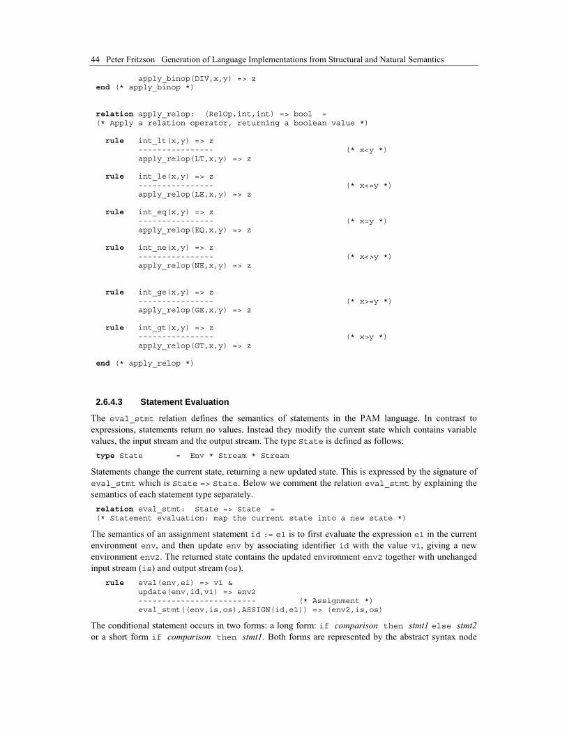
44 Peter Fritzson Generation of Language Implementations from Structural and Natural Semantics
apply_binop(DIV,x,y) => z end (* apply_binop *) relation apply_relop: (RelOp,int,int) => bool = (* Apply a relation operator, returning a boolean value *) rule int_lt(x,y) => z ---------------- (* x<y *) apply_relop(LT,x,y) => z rule int_le(x,y) => z ---------------- (* x<=y *) apply_relop(LE,x,y) => z rule int_eq(x,y) => z ---------------- (* x=y *) apply_relop(EQ,x,y) => z rule int_ne(x,y) => z ---------------- (* x<>y *) apply_relop(NE,x,y) => z rule int_ge(x,y) => z ---------------- (* x>=y *) apply_relop(GE,x,y) => z rule int_gt(x,y) => z ---------------- (* x>y *) apply_relop(GT,x,y) => z end (* apply_relop *)
2.6.4.3 Statement Evaluation
The eval_stmt relation defines the semantics of statements in the PAM language. In contrast to expressions, statements return no values. Instead they modify the current state which contains variable values, the input stream and the output stream. The type State is defined as follows: type State = Env * Stream * Stream
Statements change the current state, returning a new updated state. This is expressed by the signature of eval_stmt which is State => State. Below we comment the relation eval_stmt by explaining the semantics of each statement type separately. relation eval_stmt: State => State = (* Statement evaluation: map the current state into a new state *)
The semantics of an assignment statement id := e1 is to first evaluate the expression e1 in the current environment env, and then update env by associating identifier id with the value v1, giving a new environment env2. The returned state contains the updated environment env2 together with unchanged input stream (is) and output stream (os). rule eval(env,e1) => v1 & update(env,id,v1) => env2 ------------------------- (* Assignment *) eval_stmt((env,is,os),ASSIGN(id,e1)) => (env2,is,os)
The conditional statement occurs in two forms: a long form: if comparison then stmt1 else stmt2 or a short form if comparison then stmt1. Both forms are represented by the abstract syntax node
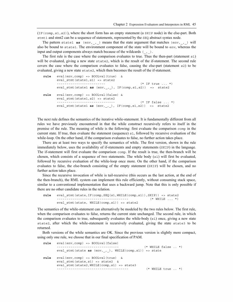
Chapter 2 Expression Evaluators and Interpreters in RML 45
(IF(comp,s1,s2)), where the short form has an empty statement (a SKIP node) in the else-part. Both stmt1 and stmt2 can be a sequence of statements, represented by the SEQ abstract syntax node.
The pattern state1 as (env,_,_) means that the state argument that matches (env,_,_) will also be bound to state1. The environment component of the state will be bound to env, whereas the input and output components always match because of the wildcards (_,_).
The first rule is the case where the comparison evaluates to true. Thus the then-part (statement s1) will be evaluated, giving a new state state2, which is the result of the if-statement. The second rule covers the case where the comparison evaluates to false, causing the else-part (statement s2) to be evaluated, giving a new state state2, which then becomes the result of the if-statement. rule eval(env,comp) => BOOLval(true) & eval_stmt(state1,s1) => state2 ------------------------- (* IF true ... *) eval_stmt(state1 as (env,_,_), IF(comp,s1,s2)) => state2 rule eval(env,comp) => BOOLval(false) & eval_stmt(state1,s2) => state2 ------------------------------ (* IF false ... *) eval_stmt(state1 as (env,_,_), IF(comp,s1,s2)) => state2
The next rule defines the semantics of the iterative while-statement. It is fundamentally different from all rules we have previously encountered in that the while construct recursively refers to itself in the premise of the rule. The meaning of while is the following: first evaluate the comparison comp in the current state. If true, then evaluate the statement (sequence) s1, followed by recursive evaluation of the while-loop. On the other hand, if the comparison evaluates to false, no further action takes place.
There are at least two ways to specify the semantics of while. The first version, shown in the rule immediately below, uses the availability of if-statements and empty statements (SKIP) in the language. The if-statement will first evaluate the comparison comp. If the result is true, the then-branch will be chosen, which consists of a sequence of two statements. The while body (s1) will first be evaluated, followed by recursive evaluation of the while-loop once more. On the other hand, if the comparison evaluates to false, the else-branch consisting of the empty statement (SKIP) will be chosen, and no further action takes place.
Since the recursive invocation of while is tail-recursive (this occurs as the last action, at the end of the then-branch), the RML system can implement this rule efficiently, without consuming stack space, similar to a conventional implementation that uses a backward jump. Note that this is only possible if there are no other candidate rules in the relation. rule eval_stmt(state,IF(comp,SEQ(s1,WHILE(comp,s1)),SKIP)) => state2 ------------------------------------- (* WHILE ... *) eval_stmt(state, WHILE(comp,s1)) => state2
The semantics of the while-statement can alternatively be modeled by the two rules below. The first rule, when the comparison evaluates to false, returns the current state unchanged. The second rule, in which the comparison evaluates to true, subsequently evaluates the while-body (s1) once, giving a new state state2, after which the while-statement is recursively evaluated, giving the state state3 to be returned.
Both versions of the while semantics are OK. Since the previous version is slightly more compact, using only one rule, we choose that in our final specification of PAM. rule eval(env,comp) => BOOLval(false) -------------------------------- (* WHILE false .. *) eval_stmt(state as (env,_,_), WHILE(comp,s1)) => state rule eval(env,comp) => BOOLval(true) & eval_stmt(state,s1) => state2 & eval_stmt(state2,WHILE(comp,s1) => state3 ------------------------------------- (* WHILE true .. *)

46 Peter Fritzson Generation of Language Implementations from Structural and Natural Semantics
eval_stmt(state as (env,_,_), WHILE(comp,s1)) => state3
The definite iterative statement: to expression do statement end first evaluates expression e1 to obtain some number n1, and provided that n1 is positive, repeatedly evaluates statement s1 the definite number of times given by n1. The repeated evaluation is performed by an auxiliary relation repeat_eval. rule eval(e1) => INTval(n1) & repeat_eval(state,n1,s1) => state2 -------------------------------------- (* TO e1 DO s1 .. *) eval_stmt(state,TODO(e1,s1)) => state2
Read and write statements modify the input and output stream components of the state, respectively. The input stream and output streams can be thought of as infinite sequences of items (for PAM: sequences of integer constants), which are handled by the operating system. First we describe the read statement.
The read statement: read id1,id2,...idN reads N values into variables id1, id2,... idN, picking them from the beginning of the input stream which is updated as a result.
The first rule covers the case of reading into an empty list of variables, which has no effect and returns the current state unchanged. The second rule models actual reading of values from the input stream. First, one item is extracted from the input stream by calling input_item, which returns a modified input stream and a value. The input_stream should be regarded as part of an abstract interface that hides the implementation of Stream. axiom eval_stmt(state,READ([])) => state (* READ [] *) rule input_item(is) => (is2,v2) & update(env,id,INTval(v2)) => env2 & eval_stmt((env2,is2,os),READ(rest)) => state2 --------------------------------------------- (* READ id1,.. *) eval_stmt((env,is,os), READ(id::rest)) => state2
Analogously, the write statement: write id1,id2,...idN writes N values from variables id1, id2,... idN, adding them to the end of the current output stream which is modified accordingly. Writing an empty list of identifiers has no effect. axiom eval_stmt(state,WRITE([])) => state (* WRITE [] *) rule lookup(env,id) => INTval(v2) & output_item(os,v2) => os2 & eval_stmt((env,is,os2),WRITE(rest)) => state2 --------------------------------------------- (* WRITE id1,..*) eval_stmt((env,is,os), WRITE(id::rest)) => state2
The semantics of a sequence stmt1; stmt2 of two statements is simple. First evaluate stmt1, giving an updated state state2. Then evaluate stmt2 in state2, giving state3 which is the resulting state. rule eval_stmt(state,stmt1) => state2 & eval_stmt(state2,stmt2) => state3 -------------------------------- (* stmt1 ; stmt2 *) eval_stmt(state,SEQ(stmt1,stmt2)) => state3
The semantics of the empty statement, represented as SKIP, is even simpler. Nothing happens, and the current state is returned unchanged. axiom eval_stmt(state,SKIP) => state (* ; empty statement *)
end (* eval_stmt *)
2.6.4.4 Auxiliary Functions
The next few subsections defines auxiliary functions (RML relations), repeat_eval, error, input_item, output_item, lookup, and update needed by the rest of the PAM specification.

Chapter 2 Expression Evaluators and Interpreters in RML 47
2.6.4.5 Repeated Statement Evaluation
The relation repeat_eval(state,n,stmt) simply evaluates the statement stmt n times, starting with state, which is updated into a new state for each iteration. The first rule specifies that nothing happens if n <= 0. The second rule checks that the counter n is greater than zero, assigns n-1 to n2, evaluates stmt in state giving a new state state2, and recursively calls repeat_eval for the remaining n-1 iterations, giving state state3. relation repeat_eval: (State, int, Stmt) => State (* repeatedly evaluate stmt n times *) rule int_le(n,0) => true ----------------------------------- (* n <= 0 *) repeat_eval(state,n,stmt) => state rule int_gt(n,0) => true &(* n > 0 *) int_sub(n,1) => n2 & eval_stmt(state,stmt) => state2 & repeat_eval(state2,n2,stmt) => state3 -------------------------------------- (* eval n times *) repeat_eval(state,n,stmt) => state3 end (* repeat_eval *)
2.6.4.6 Error Handling
The error relation can be invoked when there is some semantic error, for example when an undefined identifier is encountered. It simply prints one or two error messages, returns the empty value, and fails, which will stop evaluation (for an interpreter) or semantic analysis (for a translator). relation error: (string,string) => () = (* Print error messages str1 and str1, and fail *) rule print str1 & print str2 ------------- error(str1,str2) => fail end (* error *)
2.6.4.7 Stream I/O Primitives
The input_item relation retrieves an item (here an integer constant) from the input stream, which can be thought of as an infinite list implemented by the operating system. The item is effectively removed from the beginning of the stream, giving a new (updated) stream consisting of the rest of the list. Since Stream is implemented by the operating system, it is really an abstract data type from RML’s point of view. relation input_item (* Stream => (Stream,Item) *) (* input an item from a stream. Stream is an abstype *) (**? how to handle read? Not in RML? typing of item? *) (**? how to introduce is2? How should end-of-file be handled? Svar: antingen ??* fail (naturligare för PAM) eller använda option, men i det senare * Vid EOF, dummy-värde, eller FAIL. I Fail-fallet ger man en extra regel som * hanterar Fail-fallet); När mer info krävs, använd option. *)
rule read => item ------------------------- input_item(is) => (is2,item) end (* input_item *)
The output_item relation outputs an item by attaching the item to the front of the output stream (effectively a possibly infinite list of items), giving an updated output stream os2.

48 Peter Fritzson Generation of Language Implementations from Structural and Natural Semantics
relation output_item (* (Stream,Item) => Stream *) (* output an item. Stream is an abstype. *) (**? how should an output error be handled? How to introduce os2? *) rule print(item) --------------- output_item(os,item) => os2 end (* output_item *)
Even though Stream is an abstract data type implemented by the operating system it is also instructive to show a version of input_item and output_item that operates on streams explicitly represented as linked lists. This is shown below. (?? Stream is currently not provided by RML) relation input_item: Stream => (Stream,Item) = axiom input_item(item :: streamrest) => (streamrest,item) end (* input_item *) relation output_item: (Stream,Item) => Stream = rule list_append(item,outputstream) => outputstream2 --------------- output_item(outputstream,item) => outputstream2 end (* output_item *)
2.6.4.8 Environment Lookup and Update
The relation lookup(env,id) returns the value associated with identifier id in the environment env. If there is no binding for id in the environment, lookup will fail. Here the environment is implemented (as usual) as a linked list of (identifier,value) pairs.
The first rule covers the case where id is found in the first pair of the list. The pattern (id2,value) is concatenated (::) to the rest of the list (the pattern wildcard: _), whereas the second rule covers the case where id is not in the first pair, and therefore recursively searches the rest of the list. relation lookup: (Env,Ident) => Value = (* lookup returns the value associated with an identifier. * If no association is present, lookup will fail. *) rule id=id2 ------------------------------------- (* id first in list *) lookup((id2,value) :: _, id) => value rule not id=id2 & lookup(rest, id) => value ------------------------------------- (* id in rest of list *) lookup((id2,_) :: rest, id) => value end
The relation update(env,id,value) inserts a new binding between id and value into the environment. Here the new (id,value) pair is simply put at the beginning of the environment. If an existing binding of id was already in the environment, it will never be retrieved again because lookup performs a left-to-right search that will always encounter the new binding before the old one. relation update: (Env,Ident,Value) => Env =
axiom update(env,id,value) => ((id,value)::env)
end
2.6.4.9 The Complete Semantics for PAM
The complete semantics of PAM follows below. The relations have been sorted in a bottom-up fashion, definition-before-use, even though that is not necessary in RML. Auxiliary utility relations and low level constructs appear first, whereas statements appear last since they directly or indirectly refer to all the rest. (***************** Auxiliary utility relations ******************)
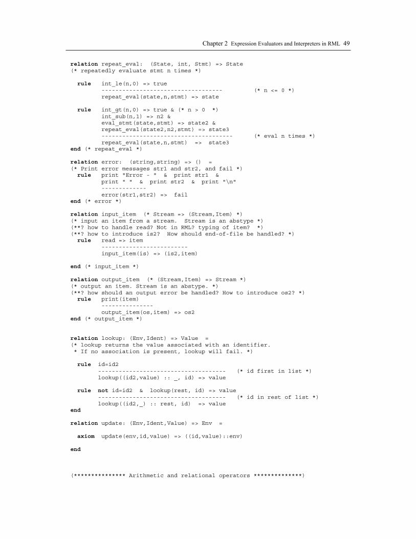
Chapter 2 Expression Evaluators and Interpreters in RML 49
relation repeat_eval: (State, int, Stmt) => State (* repeatedly evaluate stmt n times *) rule int_le(n,0) => true ----------------------------------- (* n <= 0 *) repeat_eval(state,n,stmt) => state rule int_gt(n,0) => true & (* n > 0 *) int_sub(n,1) => n2 & eval_stmt(state,stmt) => state2 & repeat_eval(state2,n2,stmt) => state3 -------------------------------------- (* eval n times *) repeat_eval(state,n,stmt) => state3 end (* repeat_eval *) relation error: (string,string) => () = (* Print error messages str1 and str2, and fail *) rule print "Error - " & print str1 & print " " & print str2 & print "\n" ------------- error(str1,str2) => fail end (* error *) relation input_item (* Stream => (Stream,Item) *) (* input an item from a stream. Stream is an abstype *) (**? how to handle read? Not in RML? typing of item? *) (**? how to introduce is2? How should end-of-file be handled? *) rule read => item ------------------------- input_item(is) => (is2,item) end (* input_item *) relation output_item (* (Stream,Item) => Stream *) (* output an item. Stream is an abstype. *) (**? how should an output error be handled? How to introduce os2? *) rule print(item) --------------- output_item(os,item) => os2 end (* output_item *) relation lookup: (Env,Ident) => Value = (* lookup returns the value associated with an identifier. * If no association is present, lookup will fail. *) rule id=id2 ------------------------------------- (* id first in list *) lookup((id2,value) :: _, id) => value rule not id=id2 & lookup(rest, id) => value ------------------------------------- (* id in rest of list *) lookup((id2,_) :: rest, id) => value end relation update: (Env,Ident,Value) => Env = axiom update(env,id,value) => ((id,value)::env) end (*************** Arithmetic and relational operators **************)
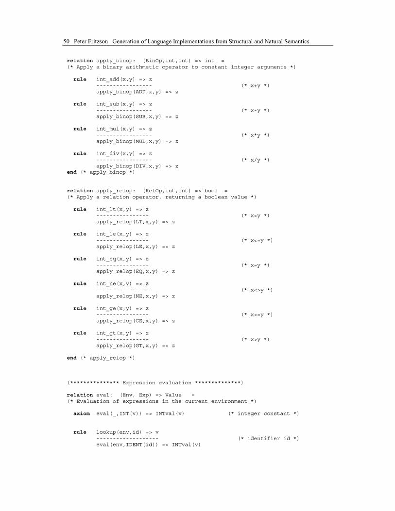
50 Peter Fritzson Generation of Language Implementations from Structural and Natural Semantics
relation apply_binop: (BinOp,int,int) => int = (* Apply a binary arithmetic operator to constant integer arguments *) rule int_add(x,y) => z ----------------- (* x+y *) apply_binop(ADD,x,y) => z rule int_sub(x,y) => z ----------------- (* x-y *) apply_binop(SUB,x,y) => z rule int_mul(x,y) => z ----------------- (* x*y *) apply_binop(MUL,x,y) => z rule int_div(x,y) => z ----------------- (* x/y *) apply_binop(DIV,x,y) => z end (* apply_binop *) relation apply_relop: (RelOp,int,int) => bool = (* Apply a relation operator, returning a boolean value *) rule int_lt(x,y) => z ---------------- (* x<y *) apply_relop(LT,x,y) => z rule int_le(x,y) => z ---------------- (* x<=y *) apply_relop(LE,x,y) => z rule int_eq(x,y) => z ---------------- (* x=y *) apply_relop(EQ,x,y) => z rule int_ne(x,y) => z ---------------- (* x<>y *) apply_relop(NE,x,y) => z rule int_ge(x,y) => z ---------------- (* x>=y *) apply_relop(GE,x,y) => z rule int_gt(x,y) => z ---------------- (* x>y *) apply_relop(GT,x,y) => z end (* apply_relop *) (*************** Expression evaluation **************) relation eval: (Env, Exp) => Value = (* Evaluation of expressions in the current environment *) axiom eval(_,INT(v)) => INTval(v) (* integer constant *) rule lookup(env,id) => v ------------------- (* identifier id *) eval(env,IDENT(id)) => INTval(v)

Chapter 2 Expression Evaluators and Interpreters in RML 51
(* If id not declared, give an error message and fail through error *) rule not lookup(env,id) => v error("Undefined identifier",id) ------------------- (* undefined variable id *) eval(env,IDENT(id)) => INTval(0) rule eval(env,e1) => INTval(v1) & eval(env,e2) => INTval(v2) & apply_binop(env,binop,v1,v2) => v3 ----------------------------------- (* expr1 binop expr2 *) eval(env, BINARY(e1,binop,e2) => INTval(v3) rule eval(env,e1) => INTval(v1) & eval(env,e2) => INTval(v2) & apply_relop(env,relop,v1,v2) => v3 ---------------------------------- (* expr1 relop expr2 *) eval(env, RELATION(e1,relop,e2) => BOOLval(v3) end (* eval *) (*************** Statement evaluation **************) relation eval_stmt: State => State = (* Statement evaluation: map the current state into a new state *) rule eval(env,e1) => v1 & update(env,id,v1) => env2 ------------------------- (* Assignment *) eval_stmt((env,is,os),ASSIGN(id,e1)) => (env2,is,os) rule eval(env,comp) => BOOLval(true) & eval_stmt(state1,s1) => state2 ------------------------- (* IF true ... *) eval_stmt(state1 as (env,_,_), IF(comp,s1,s2)) => state2 rule eval(env,comp) => BOOLval(false) & eval_stmt(state1,s2) => state2 ------------------------------ (* IF false ... *) eval_stmt(state1 as (env,_,_), IF(comp,s1,s2)) => state2 rule eval_stmt(state,IF(comp,SEQ(s1,WHILE(comp,s1)),SKIP)) => state2 ------------------------------------- (* WHILE ... *) eval_stmt(state, WHILE(comp,s1)) => state2 rule eval(env,e1) => INTval(n1) & repeat_eval(state,n1,s1) => state2 -------------------------------------- (* TO e1 DO s1 .. *) eval_stmt(state,TODO(e1,s1)) => state2 axiom eval_stmt(state,READ([])) => state (* READ [] *) rule input_item(is) => (is2,v2) & update(env,id,INTval(v2)) => env2 & eval_stmt((env2,is2,os),READ(rest)) => state2 --------------------------------------------- (* READ id1,.. *) eval_stmt((env,is,os), READ(id::rest)) => state2 axiom eval_stmt(state,WRITE([])) => state (* WRITE [] *) rule lookup(env,id) => INTval(v2) & output_item(os,v2) => os2 & eval_stmt((env,is,os2),WRITE(rest)) => state2 --------------------------------------------- (* WRITE id1,..*)
52 Peter Fritzson Generation of Language Implementations from Structural and Natural Semantics
eval_stmt((env,is,os), WRITE(id::rest)) => state2 rule eval_stmt(state,stmt1) => state2 & eval_stmt(state2,stmt2) => state3 -------------------------------- (* stmt1 ; stmt2 *) eval_stmt(state,SEQ(stmt1,stmt2)) => state3 axiom eval_stmt(state,SKIP) => state (* ; empty statement *) end (* eval_stmt *)
2.6.5 PAM Implementation – with Connection to the OS
The PAM specification referring to explicit streams as described above is useful as a semantic specification but is not very practical when generating an interpreter that actually calls the operating system to read on the standard input stream and write to the standard output stream.
Therefore we made a variant of the PAM specification without explicit modeling of the input and output streams as part of the State, using the non-declarative RML print primitive for output, and introducing a corresponding read primitive for input, implemented in C but callable from RML. This caused the following modifications to the above PAM specification: ....??
An executable PAM interpreter was generated from this semantics. An interactive example running this interpreter follows below: ...??
2.7 AssignTwoType – Introducing Typing AssignTwoType is an extension of the Assignments language made by introducing real numbers. Now we have two types in the language, integer and real, which creates a need both to check the typing of expressions during evaluation, and to be able to store constant values of two different types in the environment.
2.7.1 Concrete Syntax of AssignTwoType
Real valued constants contain a dot and/or an exponent, as in: 3.14159 5.36E-10 11E+5
Only one additional rule has been added compared to the BNF grammar of the Assignments language. The non-terminal element can now also expand into a real constant, as shown below: element : T_INTCONST | T_REALCONST | T_LPAREN expression T_RPAREN
The lexical specification follows below. One new token type, T_REALCONST, has been introduced compared to the Assignments language. The regular expression rcon1 represents a real constant that must contain a dot, whereas rcon2 must contain an exponent. Any real constant must contain either a dot or an exponent. The ? in the regular expressions signify optional occurrence.

Chapter 2 Expression Evaluators and Interpreters in RML 53
/* Lex style lexical syntax of tokens in the language AssignTwoType */ whitespace [ \t\n]+ letter [a-zA-Z_] ident {letter} ({letter} | {digit})* digit [0-9] digits {digit}+ icon {digits} pt "." sign [+-] exponent ([eE]{sign}?{digits}) rcon1 {digits}({pt}{digits}?)?{exponent} rcon2 {digits}?{pt}{digits}{exponent}? rcon {rcon1}|{rcon2} %% {whitespace} ; {ident} return lex_ident(); /* T_IDENT */ {icon} return lex_icon(); /* T_INTCONST */ {rcon} return lex_rcon(); /* T_REALCONST */ ":=" return T_ASSIGN; "+" return T_ADD; "-" return T_SUB; "*" return T_MUL; "/" return T_DIV; "(" return T_LPAREN; ")" return T_RPAREN;
2.7.2 Abstract Syntax
The abstract syntax of AssignTwoType has been extended in two ways compared to the Assignments language. A REAL node has been introduced into the expression (Exp) union type, and a parameterized abstract syntax (Section 2.3) has been selected to enable a more compact semantics part of the specification by grouping rules for similar constructs in the language.
The environment now must be able to store values of two types: integer or real. This is achieved by representing values, of type Value, as either INTval or REALval nodes. We could alternatively have used the INT and REAL constructors of the Exp union type. However, this would have had the disadvantages of mixing up the evaluation value type Value with the abstract syntax (which contain many other nodes), and making the strong typing of the specification less orthogonal, thus reducing the probability of the RML system catching possible type errors.
An auxiliary union type Ty2 has been introduced to more conveniently be able to encode the semantics of different combinations of integer and real typed values. (* Parameterized abstract syntax of the AssignTwoType language *) type Ident = string datatype BinOp = ADD | SUB | MUL | DIV datatype UnOp = NEG datatype Exp = INT of int | REAL of real | IDENT of Ident | BINARY of Exp * BinOp * Exp | UNARY of UnOp * Exp | ASSIGN of ident * Exp (* Values, bindings and environment *) datatype Value = INTval of int | REALval of real

54 Peter Fritzson Generation of Language Implementations from Structural and Natural Semantics
type VarBnd = Ident * Value type Env = VarBnd list (* Ty2 is an auxiliary datatype used to handle types during evaluation *) datatype Ty2 = INT2 of int * int | REAL2 of real * real
2.7.3 Semantics of AssignTwoType
The semantics of the AssignTwoType language is quite similar to the semantics of the Assignments language described in Section 2.5.4, except for the introduction of multiple types. Having multiple types in a language may give rise to a combinatorial explosion in the number of rules needed, because the semantics of each combination of argument types and operators needs to be described.
In order to somewhat limit this potential “explosion” of rules, we introduce a type lattice (see the next section), and use the relation type_lub (for least upper bound of types; also see the next section) which derives the resulting type and inserts possibly needed type conversions. This reduces the number of needed rules for binary operators to two: one for integer results and one for real results. The parameterized abstract syntax makes it possible to place argument evaluation and type handling for binary operators in only those two rules.
2.7.3.1 Expression Evaluation
Compared to the Assignments language, the eval relation is still quite similar. Values are now tagged by either INTval or REALval. We have inserted one additional rule for real constants, and collected all binary operators together into two rules, and unary operators into two additional rules. The rules for assignments and variable identifiers are the same as before.
We show the application of some rules to a small example, e.g: 44 + 3.14
The abstract syntax representation will be: BINARY( INT(44), ADD, REAL(3.14))
On calling eval, this will match the rule for binary operators and real number results. The first argument will be evaluated to INTval(44), bound to v1, and the second argument to REALval(3.14) bound to v2. The call to type_lub will insert a conversion of the first argument from integer to a real value, giving the result REAL2(44.0, 3.14), which also causes x to be bound to 44.0 and y to be bound to 3.14. Finally, apply_real_binop will apply the operator ADD to the two arguments, returning the result 47.14, which in the form REALval(47.14) together with the unchanged environment is the result of the call to relation eval. relation eval: (Env,Exp) => (Env,Value) = (* Evaluation of expression exp in current environment env, returning * a possibly updated environment, and a value which can be either an * integer- or real-typed constant value, tagged with constructors * INTval or REALval, respectively *) axiom eval(env, INT(ival) ) => (env,INTval(ival)) (* int constant *) axiom eval(env,REAL(rval) ) => (env,REALval(rval)) (* real constant *) rule lookupextend(env,id) => (env2,value) ----------------------------------- (* variable id *) eval(env,IDENT(id)) => (env2,value) rule eval(env,e1) => (env1,v1) & eval(env,e2) => (env2,v2) & type_lub(v1,v2) => INT2(x,y) & apply_int_binop(binop,x,y) => z

Chapter 2 Expression Evaluators and Interpreters in RML 55
-------------------------------- (* int binop int *) eval(env, BINARY(e1,binop,e2) => (env2,INTval(z)) rule eval(env,e1) => (env1,v1) & eval(env,e2) => (env2,v2) & type_lub(v1,v2) => REAL2(x,y) & apply_real_binop(binop,x,y) => z -------------------------------- (* int/real binop int/real *) eval(env, BINARY(e1,binop,e2) => (env2,REALval(z)) rule eval(env,e) => (env1,INTval(x)) & apply_int_unop(unop,x) => y ----------------------------------- (* int unop exp *) eval(env, UNARY(unop,e) ) => (env1,INTval(y)) rule eval(env,e) => (env1,REALval(x)) & apply_real_unop(unop,x) => y ------------------------------------ (* real unop exp *) eval(env, UNARY(unop,e) ) => (env1,REALval(y)) (* eval of an assignment node returns the updated environment and * the assigned value *) rule eval(env,exp) => (env1,value) & update(env1,id,value) => env2 ---------------------------------------- (* id := exp *) eval(env, ASSIGN(id,exp)) => (env2,value) (* Note: there will be no type error if a real value is assigned to an * existing integer-typed variable, since the variable will change * type when it is updated *) end (* eval *)
2.7.3.2 Type Lattice and Least Upper Bound
One general way to partially avoid the potential “combinatorial explosion” of semantic rules for different combinations of operators and types is to introduce a type lattice. The trivial type lattice for real and integer (i.e., real and int) is shown in Figure 2-4 below, using the partial order that real is greater than int since integers always can be converted to reals, but not the other way around.
real
int
lub
glb Figure 2-4. Simple type lattice for types integer and real. The least upper bound (lub) is real; the greatest lower bound (glb) is int.
We are however more interested in combinations of two argument types for binary operators, for which the following four rules apply:
• real op real => real • real op int => real • int op real => real • int op int => int
These rules are represented by the relation type_lub, introduced below. The relation is in fact doing two jobs simultaneously. It is computing the least upper bound of pairs of types, represented by the constructors INT2 or REAL2. Additionally, it performs type conversions of the arguments as needed, to ensure that both arguments become either int (for INT2) or real (for REAL2). Thus we will need only

56 Peter Fritzson Generation of Language Implementations from Structural and Natural Semantics
two sets of rules for each operator, covering the cases when both arguments are int or both arguments are real. relation type_lub (Value,Value) => Ty2 =
axiom type_lub(INTval(x), INTval(y)) => INT2(x,y) rule int_real(x) => x2 ---------------- type_lub(INTval(x), REALval(y)) => REAL2(x2,y) rule int_real(y) => y2 ----------------- type_lub(REALval(x),INTval(y)) => REAL2(x,y2) axiom type_lub(REALval(x),REALval(y)) => REAL2(x,y)
end
2.7.3.3 Binary and Unary Operators
The essential properties of binary arithmetic operators are described below in the relations apply_int_binop and apply_real_binop, respectively. Argument evaluation has been taken care of by the two rules for binary operators in relation eval, and thus need not be repeated for each rule. The type conversion needed for some combinations of real and integer values have already been described by the relation type_lub, which reduces the number of cases that need to be handled for each operator to two: either integer values (apply_int_binop) or real values (apply_real_binop). relation apply_int_binop (BinOp,int,int) => int rule int_add(x,y) => z ------------------------ (* x+y *) apply_int_binop(ADD,x,y) => z rule int_sub(x,y) => z ------------------------ (* x-y *) apply_int_binop(SUB,x,y) => z rule int_mul(x,y) => z ------------------------ (* x*y *) apply_int_binop(MUL,x,y) => z rule int_div(x,y) => z ------------------------ (* x/y *) apply_int_binop(DIV,x,y) => z end relation apply_real_binop (BinOp,real,real) => real rule real_add(x,y) => z ------------------------- (* x+y *) apply_real_binop(ADD,x,y) => z rule real_sub(x,y) => z ------------------------- (* x-y *) apply_real_binop(SUB,x,y) => z rule real_mul(x,y) => z ------------------------- (* x*y *) apply_real_binop(MUL,x,y) => z rule real_div(x,y) => z ------------------------ (* x/y *) apply_real_binop(DIV,x,y) => z
Chapter 2 Expression Evaluators and Interpreters in RML 57
end (* apply_real_binop *)
There is only one unary operator, unary minus, in the current language. Thus the relations apply_int_unop and apply_real_unop for operations on integer and real values, respectively, become rather short. relation apply_int_unop (UnOp,int) => int rule int_neg(x) => y ------------------------ (* -x *) apply_int_unop(NEG,x) => y end (* apply_int_unop *) relation apply_real_unop (UnOp,real) => real rule real_neg(x) => y ------------------------ (* -x *) apply_real_unop(NEG,x) => y end (* apply_real_unop *)
2.7.3.4 Auxiliary Relations relation lookup: (Env,Ident) => Value = (* lookup returns the value associated with an identifier. * If no association is present, lookup will fail. *) (* Identifier id is found in the first pair of the list, and value * is returned. *) rule id = id2 ------------------------------ lookup((id2,value) :: _, id) => value (* id is not found in the first pair of the list, and lookup will * recursively search the rest of the list. If found, value is returned. *) rule not id=id2 & lookup(rest, id) => value ------------------------------------- lookup((id2,_) :: rest, id) => value end (* lookup *) relation lookupextend: (Env,Ident) => (Env,Value) = (* Return value of id in env. If id not present, add id and return 0 *) rule not lookup(env,id) => v & INTval(0) = value & (id, value) :: env = env2 ----------------------------- lookupextend(env, id) => (env2,value) rule lookup(env,id) => value -------------------------------- lookupextend(env, id) => (env,value) end (* lookupextend *) relation update: (Env,Ident,Value) => Env = (* Store binding of id to value at front of environment env *) axiom update(env,id,value) => ((id,value) :: env) end (* update *)
58 Peter Fritzson Generation of Language Implementations from Structural and Natural Semantics
2.7.4 A Modular Specification of AssignTwoType
The RML module system facilitates writing modular specifications, where each module describes some related aspects of the specified language. Thus, it is common to specify the abstract syntax in a special module and other aspects such as evaluation, translation or type elaboration in separate modules.
We present a modularized version of the complete abstract syntax and semantics for AssignTwoType below, using two modules: Absyn for abstract syntax, and Eval for evaluation. Some data type declarations which are used during evaluation and are not really part of the abstract syntax, such as variable bindings and environments, have been moved to the module Eval.
The structure of an RML module is outlined below. After the module name comes an (optional) interface section, giving type definitions and signatures of relations to be exported to other modules. After the interface section comes the (optional) body of the module, containing bodies of relations and possible additional definitions that are private to the module. Some modules (e.g. Absyn) consist only of an interface part. A module may optionally import definitions from other modules, both in the interface part and in the body part. References to names defined in other modules must be prefixed by the defining module name followed by a dot, as in Absyn.ASSIGN when referencing the ASSIGN constructor from module Absyn. module modulename:
(* Interface section *) with "modulefilename1"
definition1 definition2 signature1 definition3 ..... end (* Implementation section *) with "modulefilename2" with "modulefilename3" relation relationname1 = ... ... relation relationname2 = ... ...
2.7.4.1 The Main Module
The main module implements the prompt-read-eval-print loop as the relation eval_loop, which accepts the initial (empty) environment init_env exported from module eval, and loops indefinitely. (* file: main.rml *)
module Main:
relation main: string list => ()
end with "parse.rml" with "eval.rml" relation printvalue(x)
rule print x --------------------- printvalue(INTval(x)) rule print x

Chapter 2 Expression Evaluators and Interpreters in RML 59
---------------------- printvalue(REALval(x))
end (* printvalue *) relation eval_loop: Env => () =
rule print("> ") & parse.parse_expr => ast & eval.eval_expr(env,ast) => (env2,value) & printvalue(value) & eval_loop(env2) --------------- eval_loop(env) (*** INCOMPLETE!! *) rule not parse_expr => ast & print("Syntax error in input line\n") --------------- eval_loop(env)
end (* eval_loop *) relation safe_parse_expr (**) (t.ex. via option NONE vid fel or SOME vid OK *) relation safe_eval (** om evaluering går fel; två fall eval.eval och not eval.eval vid fail *) relation main: string list => () =
rule eval_loop(eval.init_env) ------------------------ main(_)
end (* main *) (* end of module main *)
2.7.4.2 The Absyn Module (* file: absyn.rml *) (* Parameterized abstract syntax of the AssignTwoType language *) module Absyn: type Ident = string datatype BinOp = ADD | SUB | MUL | DIV datatype UnOp = NEG datatype Exp = INT of int | REAL of real | IDENT of Ident | BINARY of Exp * BinOp * Exp | UNARY of UnOp * Exp | ASSIGN of ident * Exp end (* module Absyn *)
60 Peter Fritzson Generation of Language Implementations from Structural and Natural Semantics
2.7.4.3 The Eval Module (* file eval.rml *) module Eval: with "absyn.rml" (* Values, bindings and environment *) type Value = INTval of int | REALval of real type VarBnd = Absyn.Ident * Value type Env = VarBnd list (* Initial environment is an empty list of (Ident,Value) pairs *) val init_env = [] eval: (Env,Absyn.Exp) => (Env,Value) end (* of interface section *) (* Ty2 is an auxiliary datatype used to handle types during evaluation *) datatype Ty2 = INT2 of int * int | REAL2 of real * real (*************** Auxiliary relations ***************) relation lookup: (Env,Absyn.Ident) => Value = (* lookup returns the value associated with an identifier. * If no association is present, lookup will fail. *) (* Identifier id is found in the first pair of the list, and value * is returned. *) rule id = id2 ------------------------------ lookup((id2,value) :: _, id) => value (* id is not found in the first pair of the list, and lookup will * recursively search the rest of the list. If found, value is returned. *) rule not id=id2 & lookup(rest, id) => value ------------------------------------- lookup((id2,_) :: rest, id) => value end (* lookup *) relation lookupextend: (Env,Absyn.Ident) => (Env,Value) = (* Return value of id in env. If id not present, add id and return 0 *) rule not lookup(env,id) => v & INTval(0) = value ----------------------------- lookupextend(env, id) => ((id, value)::env,value) rule lookup(env,id) => value -------------------------------- lookupextend(env, id) => (env,value) end (* lookupextend *)
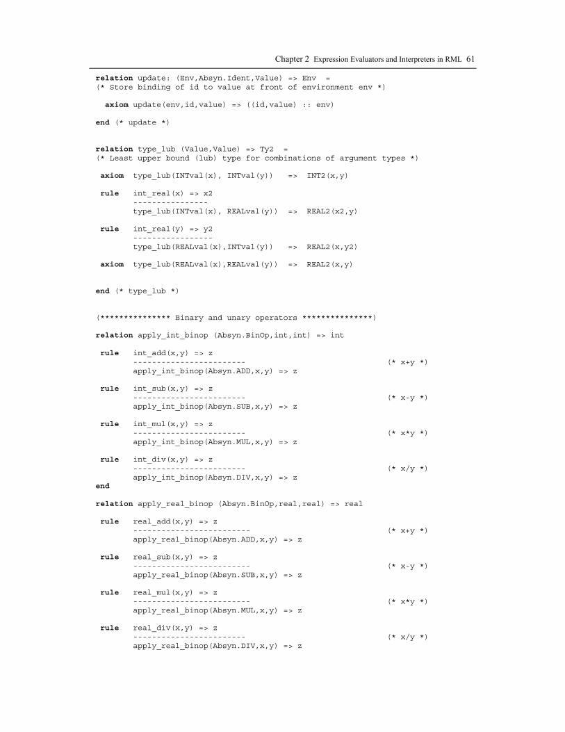
Chapter 2 Expression Evaluators and Interpreters in RML 61
relation update: (Env,Absyn.Ident,Value) => Env = (* Store binding of id to value at front of environment env *) axiom update(env,id,value) => ((id,value) :: env) end (* update *) relation type_lub (Value,Value) => Ty2 = (* Least upper bound (lub) type for combinations of argument types *) axiom type_lub(INTval(x), INTval(y)) => INT2(x,y) rule int_real(x) => x2 ---------------- type_lub(INTval(x), REALval(y)) => REAL2(x2,y) rule int_real(y) => y2 ----------------- type_lub(REALval(x),INTval(y)) => REAL2(x,y2) axiom type_lub(REALval(x),REALval(y)) => REAL2(x,y) end (* type_lub *) (*************** Binary and unary operators ***************) relation apply_int_binop (Absyn.BinOp,int,int) => int rule int_add(x,y) => z ------------------------ (* x+y *) apply_int_binop(Absyn.ADD,x,y) => z rule int_sub(x,y) => z ------------------------ (* x-y *) apply_int_binop(Absyn.SUB,x,y) => z rule int_mul(x,y) => z ------------------------ (* x*y *) apply_int_binop(Absyn.MUL,x,y) => z rule int_div(x,y) => z ------------------------ (* x/y *) apply_int_binop(Absyn.DIV,x,y) => z end relation apply_real_binop (Absyn.BinOp,real,real) => real rule real_add(x,y) => z ------------------------- (* x+y *) apply_real_binop(Absyn.ADD,x,y) => z rule real_sub(x,y) => z ------------------------- (* x-y *) apply_real_binop(Absyn.SUB,x,y) => z rule real_mul(x,y) => z ------------------------- (* x*y *) apply_real_binop(Absyn.MUL,x,y) => z rule real_div(x,y) => z ------------------------ (* x/y *) apply_real_binop(Absyn.DIV,x,y) => z

62 Peter Fritzson Generation of Language Implementations from Structural and Natural Semantics
end (* apply_real_binop *) relation apply_int_unop (UnOp,int) => int rule int_neg(x) => y ------------------------ (* -x *) apply_int_unop(Absyn.NEG,x) => y end (* apply_int_unop *) relation apply_real_unop (UnOp,real) => real rule real_neg(x) => y ------------------------ (* -x *) apply_real_unop(Absyn.NEG,x) => y end (* apply_real_unop *) (*************** Expression evaluation ***************) relation eval: (Env,Exp) => (Env,Value) = (* Evaluation of expression exp in current environment env, returning * a possibly updated environment, and a value which can be either an * integer- or real-typed constant value, tagged with constructors * INTval or REALval, respectively *) axiom eval(env,Absyn.INT(ival)) => (env,INTval(ival)) (* int const *) axiom eval(env,Absyn.REAL(rval)) => (env,REALval(rval)) (* real const *) rule lookupextend(env,id) => (env2,value) ----------------------------------- (* variable id *) eval(env,Absyn.IDENT(id)) => (env2,value) rule eval(env,e1) => (env1,v1) & eval(env,e2) => (env2,v2) & type_lub(v1,v2) => INT2(x,y) & apply_int_binop(binop,x,y) => z -------------------------------- (* int binop int *) eval(env, Absyn.BINARY(e1,binop,e2) => (env2,INTval(z)) rule eval(env,e1) => (env1,v1) & eval(env,e2) => (env2,v2) & type_lub(v1,v2) => REAL2(x,y) & apply_real_binop(binop,x,y) => z -------------------------------- (* int/real binop int/real *) eval(env, Absyn.BINARY(e1,binop,e2) => (env2,REALval(z)) rule eval(env,e) => (env1,INTval(x)) & apply_int_unop(unop,x) => y ----------------------------------- (* int unop exp *) eval(env, Absyn.UNARY(unop,e) ) => (env1,INTval(y)) rule eval(env,e) => (env1,REALval(x)) & apply_real_unop(unop,x) => y ------------------------------------ (* real unop exp *) eval(env, Absyn.UNARY(unop,e) ) => (env1,REALval(y)) (* eval of an assignment node returns the updated environment and * the assigned value *)

Chapter 2 Expression Evaluators and Interpreters in RML 63
rule eval(env,exp) => (env1,value) & update(env1,id,value) => env2 ---------------------------------------- (* id := exp *) eval(env, Absyn.ASSIGN(id,exp)) => (env2,value) (* Note: there will be no type error if a real value is assigned to an * existing integer-typed variable, since the variable will change * type when it is updated. *) end (* eval *) (* End of module Eval *)
2.8 The PAMDECL Language PAMDECL is PAM extended with declarations of variables and two types: integer and real. Thus it combines the properties of both PAM and AssignTwoType. The specification is modular, including separate modules for abstract syntax (Absyn), environment handling (Env) and evaluation (Eval). (*?? Give explanations about the various components of PAMDECL *)
2.8.1 Absyn
sdfsdf?? module Absyn: datatype BinOp = ADD | SUB | MUL | DIV datatype UnOp = NEG datatype RelOp = LT | LE | GT | GE | NE | EQ type Ident = string datatype Expr = INTCONST of int | REALCONST of real | BINARY of Expr * BinOp * Expr | UNARY of UnOp * Expr | RELATION of Expr * RelOp * Expr | VARIABLE of Ident datatype Stmt = ASSIGN of Ident * Expr | WRITE of Expr | NOOP | IF of Expr * Stmt list * Stmt list | WHILE of Expr * Stmt list type StmtList = Stmt list datatype Decl = NAMEDECL of Ident * Ident type DeclList = Decl list datatype Prog = PROG of DeclList * StmtList end
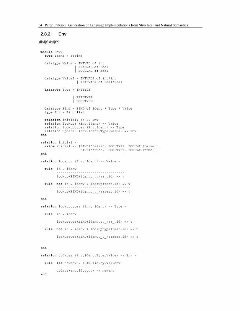
64 Peter Fritzson Generation of Language Implementations from Structural and Natural Semantics
2.8.2 Env
slkdjflskdjf?? module Env: type Ident = string datatype Value = INTVAL of int | REALVAL of real | BOOLVAL of bool datatype Value2 = INTVAL2 of int*int | REALVAL2 of real*real datatype Type = INTTYPE | REALTYPE | BOOLTYPE datatype Bind = BIND of Ident * Type * Value type Env = Bind list relation initial: () => Env relation lookup: (Env,Ident) => Value relation lookuptype: (Env,Ident) => Type relation update: (Env,Ident,Type,Value) => Env end relation initial = axiom initial => [BIND("false", BOOLTYPE, BOOLVAL(false)), BIND("true", BOOLTYPE, BOOLVAL(true))] end relation lookup: (Env, Ident) => Value = rule id = idenv ---------------------------------- lookup(BIND(idenv,_,v)::_,id) => v rule not id = idenv & lookup(rest,id) => v ------------------------------------- lookup(BIND(idenv,_,_)::rest,id) => v end relation lookuptype: (Env, Ident) => Type = rule id = idenv -------------------------------------- lookuptype(BIND(idenv,t,_)::_,id) => t rule not id = idenv & lookuptype(rest,id) => t ----------------------------------------- lookuptype(BIND(idenv,_,_)::rest,id) => t end relation update: (Env,Ident,Type,Value) => Env = rule let newenv = (BIND(id,ty,v)::env) ----------------------------- update(env,id,ty,v) => newenv end

Chapter 2 Expression Evaluators and Interpreters in RML 65
2.8.3 Eval
??lkjlkjlkjkj module Eval: with "absyn.rml" with "env.rml" relation evalprog: (Absyn.Prog) => () end (* Type lattice; int --> real *) relation binary_lub: (Env.Value,Env.Value) => Env.Value2 = axiom binary_lub(Env.INTVAL v1, Env.INTVAL(v2)) => Env.INTVAL2(v1,v2) axiom binary_lub(Env.REALVAL(v1), Env.REALVAL(v2)) => Env.REALVAL2(v1,v2) rule int_real(v1) => c1 ------------------------------------------------------------------- binary_lub(Env.INTVAL(v1), Env.REALVAL(v2)) => Env.REALVAL2(c1,v2) rule int_real(v2) => c2 ------------------------------------------------------------------- binary_lub(Env.REALVAL(v1), Env.INTVAL(v2)) => Env.REALVAL2(v1,c2) end
(* Promotion and type check *)
relation promote: (Env.Value, Env.Type) => Env.Value = axiom promote(Env.INTVAL(v), Env.INTTYPE) => Env.INTVAL(v) axiom promote(Env.REALVAL(v), Env.REALTYPE) => Env.REALVAL(v) axiom promote(Env.BOOLVAL(v), Env.BOOLTYPE) => Env.BOOLVAL(v) rule int_real(v) => v2 ----------------------------------------------------- promote(Env.INTVAL(v), Env.REALTYPE) => Env.REALVAL(v2) end (* Auxiliary functions for applying the binary operators *) relation apply_int_binary: (Absyn.BinOp, int, int) => int = rule int_add(v1,v2) => v3 --------------------------------------- apply_int_binary(Absyn.ADD,v1,v2) => v3 rule int_sub(v1,v2) => v3 --------------------------------------- apply_int_binary(Absyn.SUB,v1,v2) => v3 rule int_mul(v1,v2) => v3 --------------------------------------- apply_int_binary(Absyn.MUL,v1,v2) => v3

66 Peter Fritzson Generation of Language Implementations from Structural and Natural Semantics
rule int_div(v1,v2) => v3 --------------------------------------- apply_int_binary(Absyn.DIV,v1,v2) => v3 end relation apply_real_binary: (Absyn.BinOp, real, real) => real = rule real_add(v1,v2) => v3 ---------------------------------------- apply_real_binary(Absyn.ADD,v1,v2) => v3 rule real_sub(v1,v2) => v3 ---------------------------------------- apply_real_binary(Absyn.SUB,v1,v2) => v3 rule real_mul(v1,v2) => v3 ---------------------------------------- apply_real_binary(Absyn.MUL,v1,v2) => v3 rule real_div(v1,v2) => v3 ---------------------------------------- apply_real_binary(Absyn.DIV,v1,v2) => v3 end (* Auxiliary functions for applying the unary operators *) relation apply_int_unary: (Absyn.UnOp, int) => int = rule int_neg v1 => v2 ----------------------------------- apply_int_unary(Absyn.NEG,v1) => v2 end relation apply_real_unary: (Absyn.UnOp, real) => real = rule real_neg v1 => v2 ------------------------------------ apply_real_unary(Absyn.NEG,v1) => v2 end (* Auxiliary functions for applying the relation operators *) relation apply_int_relation: (Absyn.RelOp, int, int) => bool = rule int_lt(v1,v2) => v3 ---------------------------------------- apply_int_relation(Absyn.LT,v1,v2) => v3 rule int_le(v1,v2) => v3 ---------------------------------------- apply_int_relation(Absyn.LE,v1,v2) => v3 rule int_gt(v1,v2) => v3 ---------------------------------------- apply_int_relation(Absyn.GT,v1,v2) => v3 rule int_ge(v1,v2) => v3 ---------------------------------------- apply_int_relation(Absyn.GE,v1,v2) => v3 rule int_ne(v1,v2) => v3 ---------------------------------------- apply_int_relation(Absyn.NE,v1,v2) => v3

Chapter 2 Expression Evaluators and Interpreters in RML 67
rule int_eq(v1,v2) => v3 ---------------------------------------- apply_int_relation(Absyn.EQ,v1,v2) => v3 end
relation apply_real_relation: (Absyn.RelOp, real, real) => bool = rule real_lt(v1,v2) => v3 ----------------------------------------- apply_real_relation(Absyn.LT,v1,v2) => v3 rule real_le(v1,v2) => v3 ----------------------------------------- apply_real_relation(Absyn.LE,v1,v2) => v3 rule real_gt(v1,v2) => v3 ----------------------------------------- apply_real_relation(Absyn.GT,v1,v2) => v3 rule real_ge(v1,v2) => v3 ----------------------------------------- apply_real_relation(Absyn.GE,v1,v2) => v3 rule real_ne(v1,v2) => v3 ----------------------------------------- apply_real_relation(Absyn.NE,v1,v2) => v3 rule real_eq(v1,v2) => v3 ----------------------------------------- apply_real_relation(Absyn.EQ,v1,v2) => v3 end (* EVALUATE A SINGLE EXPRESSION in an environment. Return the new value. Expressions do not change environments. *) relation eval_expr: (Env.Env, Absyn.Expr) => Env.Value = (* Constants *) axiom eval_expr(env,Absyn.INTCONST(v)) => Env.INTVAL(v) axiom eval_expr(env,Absyn.REALCONST(v)) => Env.REALVAL(v) (* Binary operators *) rule eval_expr(env,e1) => v1 & eval_expr(env,e2) => v2 & binary_lub(v1,v2) => Env.INTVAL2(c1,c2) & apply_int_binary(binop,c1,c2) => v3 --------------------------------------------------------- eval_expr(env,Absyn.BINARY(e1,binop,e2)) => Env.INTVAL(v3) rule eval_expr(env,e1) => v1 & eval_expr(env,e2) => v2 & binary_lub(v1,v2) => Env.REALVAL2(c1,c2) & apply_real_binary(binop,c1,c2) => v3 --------------------------------------------------------- eval_expr(env,Absyn.BINARY(e1,binop,e2)) => Env.REALVAL(v3) rule print "Error: binary operator applied to invalid type(s)\n" ------------------------------------------------------------- eval_expr(_,Absyn.BINARY(_,_,_)) => fail (* Unary operators *)

68 Peter Fritzson Generation of Language Implementations from Structural and Natural Semantics
rule eval_expr(env,e1) => Env.INTVAL(v1) & apply_int_unary(unop,v1) => v2 ---------------------------------------------------- eval_expr(env,Absyn.UNARY(unop,e1)) => Env.INTVAL(v2) rule eval_expr(env,e1) => Env.REALVAL(v1) & apply_real_unary(unop,v1) => v2 ----------------------------------------------------- eval_expr(env,Absyn.UNARY(unop,e1)) => Env.REALVAL(v2) rule print "Error: unary operator applied to invalid type\n" --------------------------------------------------------- eval_expr(_,Absyn.UNARY(_,_)) => fail (* Relation operators *) rule eval_expr(env,e1) => v1 & eval_expr(env,e2) => v2 & binary_lub(v1,v2) => Env.INTVAL2(c1,c2) & apply_int_relation(relop,c1,c2) => v3 --------------------------------------------------------- eval_expr(env,Absyn.RELATION(e1,relop,e2)) => Env.BOOLVAL(v3) rule eval_expr(env,e1) => v1 & eval_expr(env,e2) => v2 & binary_lub(v1,v2) => Env.REALVAL2(c1,c2) & apply_real_relation(relop,c1,c2) => v3 --------------------------------------------------------- eval_expr(env,Absyn.RELATION(e1,relop,e2)) => Env.BOOLVAL(v3) rule print "Error: relation operator applied to invalid type(s)\n" --------------------------------------------------------------- eval_expr(_,Absyn.RELATION(_,_,_)) => fail (* Variable lookup *) rule Env.lookup(env,id) => v -------------------------------------- eval_expr(env,Absyn.VARIABLE(id)) => v rule not Env.lookup(env,id) => v & print "Error: undefined variable (" & print id & print ")\n" -------------------------------------------------------------- eval_expr(env,Absyn.VARIABLE(id)) => fail end (* EVALUATING STATEMENTS *) (* Print a value - the "write" statement *) relation print_value: Env.Value => () = rule int_string(v) => vstr & print(vstr) & print("\n") ------------------------ print_value(Env.INTVAL(v)) rule real_string(v) => vstr & print(vstr) & print("\n") ------------------------- print_value(Env.REALVAL(v))

Chapter 2 Expression Evaluators and Interpreters in RML 69
rule print "true\n" ---------------------------- print_value(Env.BOOLVAL(true)) rule print "false\n" ----------------------------- print_value(Env.BOOLVAL(false)) end (* Evaluate a single statement. Pass environment forward.*) relation eval_stmt: (Env.Env,Absyn.Stmt) => Env.Env = rule eval_expr(env,e) => v & Env.lookuptype(env,id) => ty & promote(v,ty) => v2 & Env.update(env,id,ty,v2) => env1 ----------------------------------------- eval_stmt(env,Absyn.ASSIGN(id,e)) => env1 rule eval_expr(env,e) => v & print "Error: assignment mismatch or variable missing\n" ---------------------------------------------------------- eval_stmt(env,Absyn.ASSIGN(id,e)) => fail rule eval_expr(env,e) => v & print_value(v) ------------------------------------ eval_stmt(env,Absyn.WRITE(e)) => env axiom eval_stmt(env,Absyn.NOOP) => env rule eval_expr(env,e) => Env.BOOLVAL(true) & eval_stmt_list(env,c) => env1 -------------------------------------- eval_stmt(env,Absyn.IF(e,c,_)) => env1 rule eval_expr(env,e) => Env.BOOLVAL(false) & eval_stmt_list(env,a) => env1 --------------------------------------- eval_stmt(env,Absyn.IF(e,_,a)) => env1 rule eval_expr(env,e) => Env.BOOLVAL(true) & eval_stmt_list(env,ss) => env1 & eval_stmt(env1,Absyn.WHILE(e,ss)) => env2 ----------------------------------------- eval_stmt(env,Absyn.WHILE(e,ss)) => env2 rule eval_expr(env,e) => Env.BOOLVAL(false) --------------------------------------- eval_stmt(env,Absyn.WHILE(e,ss)) => env rule eval_expr(env,e) => Env.BOOLVAL(false) & eval_stmt_list(env,a) => env1 --------------------------------------- eval_stmt(env,Absyn.IF(e,_,a)) => env1 rule eval_expr(env,e) => Env.BOOLVAL(true) & eval_stmt_list(env,ss) => env1 & eval_stmt(env1,Absyn.WHILE(e,ss)) => env2 ----------------------------------------- eval_stmt(env,Absyn.WHILE(e,ss)) => env2

70 Peter Fritzson Generation of Language Implementations from Structural and Natural Semantics
rule eval_expr(env,e) => Env.BOOLVAL(false) --------------------------------------- eval_stmt(env,Absyn.WHILE(e,ss)) => env end (* Evaluate a list of statements in an environent. Pass environment forward *) relation eval_stmt_list: (Env.Env,Absyn.StmtList) => Env.Env = axiom eval_stmt_list(env,nil) => env rule eval_stmt(env,s) => env1 & eval_stmt_list(env1,ss) => env2 --------------------------------- eval_stmt_list(env,(s::ss)) => env2 end (* EVALUATING DECLARATIONS *) (* Evaluate a single statement. Pass environment forward.*) relation eval_decl: (Env.Env,Absyn.Decl) => Env.Env = rule Env.update(env,var,Env.INTTYPE, Env.INTVAL(0)) => env2 ----------------------------------------------------- eval_decl(env,Absyn.NAMEDECL(var,"integer")) => env2 rule Env.update(env,var,Env.REALTYPE, Env.REALVAL(0.0)) => env2 --------------------------------------------------------- eval_decl(env,Absyn.NAMEDECL(var,"real")) => env2 rule Env.update(env,var,Env.BOOLTYPE, Env.BOOLVAL(false)) => env2 ----------------------------------------------------------- eval_decl(env,Absyn.NAMEDECL(var,"boolean")) => env2 end (* Evaluate a list of declarations, extending the environent. *) relation eval_decl_list: (Env.Env,Absyn.DeclList) => Env.Env = axiom eval_decl_list(env,nil) => env rule eval_decl(env,s) => env1 & eval_decl_list(env1,ss) => env2 --------------------------------- eval_decl_list(env,(s::ss)) => env2 end (* EVALUTATING A PROGRAM means to evaluate the list of statements, with an initial environment containing just standard defs. *) relation evalprog: Absyn.Prog => () = rule Env.initial => env1 & eval_decl_list(env1,decls) => env2 & eval_stmt_list(env2,stmts) => env3 ------------------------------------ evalprog(Absyn.PROG(decls,stmts)) => ()

Chapter 2 Expression Evaluators and Interpreters in RML 71
end
2.9 Summary In this chapter we have used a sequence of small example languages to introduce RML together with techniques for programming language specification in Structured Operational Semantics. We started with the very simple Exp1 language, containing simple integer arithmetic and integer constants. Then follows a short section on the parameterized style of abstract syntax.The Exp2 specification describes the same language as Exp1 but shows the consequences of using parameterized abstract syntax. The Assignments language extends Exp1 with variables and assignments, thus introducing the concept of environment.
The small Pascal-like PAM language further extends our toy language by introducing control structures such as if-then-else statements, loops (but not goto), and simple input/input. However, PAM does not include procedures and multiple variable types. Only integer variables are handled by the produced evaluator. PAM also introduces relational expressions. Parameterized abstract syntax is used in the specification.
Our next language, called AssignTwoType, is designed to introduce multiple variable types in the language. It is the same language as Assignments, but adding real values and variables, and employing the parameterized style of abstract syntax. The concept of type lattice is also introduced in this section.
Next, we present the concept of RML modules, which is applied to a modular version of AssignTwoType to show how different aspects of a specification such as abstract syntax, environment handling, evaluation rules, etc. can be separated in different modules. Such modularization is especially important for large specifications.
Finally, we combine the constructs of the PAM language, the multiple variable types of AssignTwoType and the usage of RML modules, to produce a modular specification of a language called PAMDECL, which is PAM extended with declarations and multiple (integer and real) variable types.
The style of all specifications so far have been “evaluative” in nature, aiming at producing interpreters. In Chapter 5 we will present “translational” style specifications, from which compilers can be generated.
(BRK)


73
Chapter 3 Getting Started with the RML System
This chapter provides information about a number of technical details that the reader will need to know in order to get started using the RML system. This includes information about where the RML system resides, how to invoke the rml2c program generator, how to compile and link generated code, how to run the RML debugger, etc.
In order to keep the presentation concise, we return to the simplest of all language examples described so far—the expression language Exp1 presented at the beginning of Chapter 2. We will show how to build and run a working calculator that can evaluate constant arithmetic expressions expressed in the Exp1 language. We will also describe how to build an interpreter for a larger language—the PAMDECL language described in Section 2.8.
3.1 Path and Locations of Needed Files Before one can use the RML system a few changes in the environment need to be done. Note that these changes are non portable and will only work at the Department of Computer and Information Science at Linköping University, Sweden.
In order to get the correct settings for the RML environment one need to add some modules. module initadd labs/pelab pelab-before pelab-pub-before rml (?? Sun Solaris only)
The module labs/pelab sets up the module path. In order to run an emacs that supports the RML-mode pelab-before is added. The module rml sets up the RML environment. Two environment variables are set by the rml module: the variable RMLHOME, which is set to the directory where the complete system of RML resides and RMLRUNTIME which is set to the directory of the RML runtime files (bin, lib and include) for sparc solaris2 is located.
To set import the RML emacs mode rml-mode write the following as the first thing in your .emacs file: (?? Sun Solaris??) (setq load-path (cons (expand-file-name (concat (getenv "RMLHOME") "/elisp")) load-path))
The tools lex and yacc can be found in /user/ccs/bin, but if the paths have been set up correctly one need not worry about this.
The reader may copy the example files from the /home/pelab/pub/pkg/rml/current/ bookexamples directory or type them in from the examples in this chapter. Preferrably copy the whole directory with the command: cp -r /home/pelab/pub/pkg/rml/current/bookexamples/ ./myrmlexamples

74 Peter Fritzson Generation of Language Implementations from Structural and Natural Semantics
3.2 The Exp1 Calculator Again
3.2.1 Running the Exp1 Calculator
Before building the Exp1 calculator it is instructive to show how it can be used. The executable has been named calc, and is invoked by just typing calc at the Unix command prompt (sen20%10). Input typed by the user is shown in boldface.
First type calc to invoke the calculator, which responds with some trace printout to show that it has initialized and has started parsing text read from the command line.
Then type the expression to be evaluated (here: -5+10-2), followed by pushing the Enter key and typing ctrl-D (^D). The ctrl-D is needed to close the input file (which here is a “terminal”), since the Yacc-generated parser currently expects to read a whole input file before completing the parsing. Finally a trace printout ([Calc]) from the evaluator is printed, together with the result (3) of evaluating the expression. (?? this description is only valid for a Unix or Linux shell??) sen20%10 calc [Init] [Parse] -5+10-2 ^D[Eval]
Result: 3
The following example shows how the calculator reacts when it is fed an expression which does not belong to the Exp1 expression language. Remember that this language only allows simple arithmetic expressions not including variables or symbolic constants. sen20%11 calc [Init] [Parse] hej+5 Syntax error at or near line 1. Parsing failed!
3.2.2 Building the Exp1 Calculator
Before building the Exp1 calculator, we need to locate the RML, Lex and Yacc tools. It is useful for the reader who wishes to test building and running the calculator to create his/her own work directory (e.g. called myexp1).
3.2.2.1 Source Files to be Provided
Three files are needed to specify all properties (syntax and semantics) of the Exp1 language. One additional file defines the main program.
• The file exp1.rml contains an interpretive style Structured Operational Semantics specification and abstract syntax of the Exp1 language in RML form, here within the single RML module Exp1.
• The file parser.y contains the grammar of the Exp1 language in Yacc-style BNF form. • The file lexer.l specifies the lexical syntax of tokens in the Exp1 language in Lex-style regular
expression form. • In addition, a file main.c defines the C main program that calls initialization routines, the
generated scanner, parser and evaluator, and prints the evaluated result.

Chapter 3 Getting Started with the RML System 75
3.2.2.2 Generated Source Files
The following five files are generated by the RML system and the Yacc and Lex tools, respectively:
• The files exp1.c and exp1.h are generated by the rml2c translator. The generated C code that performs evaluation of Exp1 expressions can be found in exp1.c, whereas exp1.h contains tree-building macros to be called by the parser to build abstract syntax trees of input expressions that are passed to the evaluator.
• The files parser.c and parser.h are generated by Yacc, and contain a parser for Exp1 and token definitions, respectively.
• The file lexer.c is generated by Lex, and contains a scanner for Exp1.
3.2.2.3 Library File(s)
The following system specific library files and header files are also needed. (?? Unix only??)
• The files yacclib.c and yacclib.h contain some basic primitive routines needed in the course of building abstract syntax tree nodes during parsing. Most of these routines are not called directly by the user. Instead they are typically invoked via the tree building macros defined in exp1.h. Some routines (e.g. mk_icon, mk_rcon, mk_scon, mk_nil) for building RML-type integer, real and string constants, and a nil pointer, are also defined in yacclib.c.
• The file rml.h contains definitions and macros for calling the RML runtime system and predefined functions (located in $RMLRUNTIME/include/plain).
• The file librml.a is a library of all RML runtime system routines and predefined functions (located in $RMLRUNTIME/lib/plain).
3.2.2.4 Makefile for Building the Exp1 Calculator
Building the Exp1 calculator from the needed components is conveniently described by a Makefile, such as the one below. The gnu C compiler (gcc) is used here. Library files and header files are found in $RMLRUNTIME/{include,lib} if not available in the current directory. The usual make dependencies are specified. The command: make calc
will build the binary executable of the calculator (called calc) whereas the command: make clean
will remove all generated files, object files and the binary executable file. # Makefile for building the Exp1 calculator # # ??Note: LDFLAGS, CFLAGS are non-portable for some Unix systems # VARIABLES SHELL = /bin/sh LDLIBS = -ll -lrml LDFLAGS = -L$(RMLRUNTIME)/lib/plain/ CC = gcc CFLAGS = -I$(RMLRUNTIME)/include/plain/ -g # EVERYTHING all: calc # MAIN PROGRAM CALCOBJS= main.o lexer.o parser.o yacclib.o exp1.o

76 Peter Fritzson Generation of Language Implementations from Structural and Natural Semantics
calc: $(CALCOBJS) $(CC) $(LDFLAGS) $(CALCOBJS) $(LDLIBS) -o calc main.o: main.c exp1.h # LEXER lexer.o: lexer.c parser.h exp1.h lexer.c: lexer.l lex -t lexer.l >lexer.c # PARSER parser.o: parser.c exp1.h parser.c parser.h: parser.y yacc -d parser.y mv y.tab.c parser.c mv y.tab.h parser.h # ABSTRACT SYNTAX and EVALUATION exp1.o: exp1.c exp1.c exp1.h: exp1.rml rml2c -c exp1.rml # AUX clean: -rm calc $(CALCOBJS) lexer.c parser.c parser.h exp1.c exp1.h
3.2.3 Source Files for the Exp1 Calculator
Below we present the three source files lexer.l, parser.y, and exp1.rml, needed to specify the syntax and semantics of the Exp1 language, as well as the main program file main.c.
3.2.3.1 Lexical Syntax: lexer.l
The file lexer.l defines the lexical syntax of the Exp1 language, identical to what was presented in Section 2.1.1, but augmented by mentioning necessary include files.
The global variable yylval is used to transmit the values of tokens that have values—such as integer constants (T_INTCONST)—to the parser.
Character sequences including new line (\n) which cannot give rise to legal tokens in Exp1 are taken care of by junk, which is just skipped.
The routine exp1__INTconst in exp1.h builds abstract syntax integer leaf nodes and is generated by rml2c when processing the abstract syntax definitions in exp1.rml.
The routine mk_icon (from yacclib.h) builds RML compatible integer constants that can be passed to RML constructors such as exp1.INTconst, here callable as exp1__INTconst. /* file lexer.l */ %{ #include "parser.h" #include "yacclib.h" #include "rml.h" #include "exp1.h" typedef void *rml_t; extern rml_t yylval; rml_t absyn_integer(char *s);

Chapter 3 Getting Started with the RML System 77
%} digit ("0"|"1"|"2"|"3"|"4"|"5"|"6"|"7"|"8"|"9") digits {digit}+ junk .|\n %% {digits} { yylval=absyn_integer(yytext); return T_INTCONST;} "+" return T_ADD; "-" return T_SUB; "*" return T_MUL; "/" return T_DIV; "(" return T_LPAREN; ")" return T_RPAREN; {junk}+ ; %% rml_t absyn_integer(char *s) { return (rml_t) exp1__INTconst(mk_icon(atoi(s))); }
3.2.3.2 Grammar: parser.y
The grammar file parser.y follows below. The grammar rules are identical to those presented in Section 2.1.1. However, some include files are mentioned here and tree-building calls have been inserted at the parser rules in order to build the abstract syntax tree during parsing.
The tree building routines exp1__ADDop, exp1__SUBop, exp1__MULop, exp1__DIVop, exp1__NEGop, and exp1__INTconst are generated by rml2c from the definition of the Exp1 abstract syntax in the module exp1 that can be found in the file exp1.rml. The definition of these can be found in exp1.h. Leaf nodes such as INTconst are returned by the scanner. /* file parser.y */ %{ #include <stdio.h> #include "yacclib.h" #include "rml.h" #include "exp1.h" typedef void *rml_t; #define YYSTYPE rml_t extern rml_t absyntree; %} %token T_INTCONST %token T_LPAREN T_RPAREN %token T_ADD %token T_SUB %token T_MUL %token T_DIV %token T_GARBAGE %% /* Yacc BNF Syntax of the expression language Exp1 */ program : expression { absyntree = $1; }
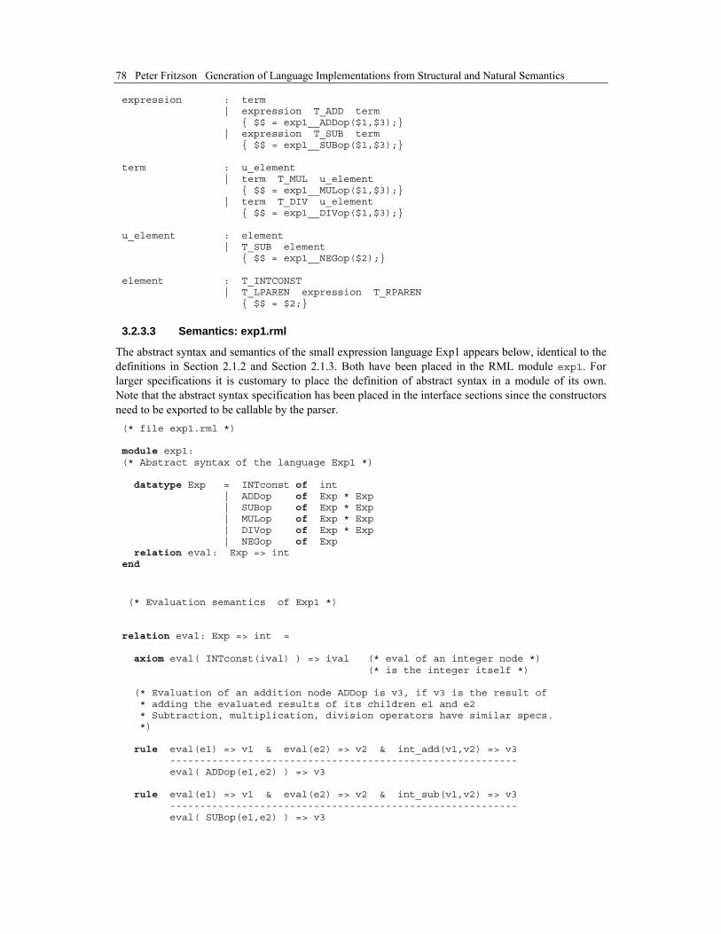
78 Peter Fritzson Generation of Language Implementations from Structural and Natural Semantics
expression : term | expression T_ADD term { $$ = exp1__ADDop($1,$3);} | expression T_SUB term { $$ = exp1__SUBop($1,$3);} term : u_element | term T_MUL u_element { $$ = exp1__MULop($1,$3);} | term T_DIV u_element { $$ = exp1__DIVop($1,$3);} u_element : element | T_SUB element { $$ = exp1__NEGop($2);} element : T_INTCONST | T_LPAREN expression T_RPAREN { $$ = $2;}
3.2.3.3 Semantics: exp1.rml
The abstract syntax and semantics of the small expression language Exp1 appears below, identical to the definitions in Section 2.1.2 and Section 2.1.3. Both have been placed in the RML module exp1. For larger specifications it is customary to place the definition of abstract syntax in a module of its own. Note that the abstract syntax specification has been placed in the interface sections since the constructors need to be exported to be callable by the parser. (* file exp1.rml *) module exp1: (* Abstract syntax of the language Exp1 *) datatype Exp = INTconst of int | ADDop of Exp * Exp | SUBop of Exp * Exp | MULop of Exp * Exp | DIVop of Exp * Exp | NEGop of Exp relation eval: Exp => int end
(* Evaluation semantics of Exp1 *) relation eval: Exp => int = axiom eval( INTconst(ival) ) => ival (* eval of an integer node *) (* is the integer itself *) (* Evaluation of an addition node ADDop is v3, if v3 is the result of * adding the evaluated results of its children e1 and e2 * Subtraction, multiplication, division operators have similar specs. *) rule eval(e1) => v1 & eval(e2) => v2 & int_add(v1,v2) => v3 ---------------------------------------------------------- eval( ADDop(e1,e2) ) => v3 rule eval(e1) => v1 & eval(e2) => v2 & int_sub(v1,v2) => v3 ---------------------------------------------------------- eval( SUBop(e1,e2) ) => v3
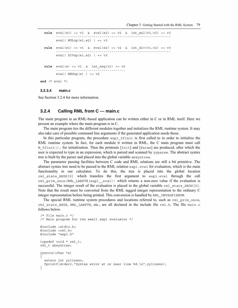
Chapter 3 Getting Started with the RML System 79
rule eval(e1) => v1 & eval(e2) => v2 & int_mul(v1,v2) => v3 ---------------------------------------------------------- eval( MULop(e1,e2) ) => v3 rule eval(e1) => v1 & eval(e2) => v2 & int_div(v1,v2) => v3 ---------------------------------------------------------- eval( DIVop(e1,e2) ) => v3 rule eval(e) => v1 & int_neg(v1) => v2 ----------------------------------- eval( NEGop(e) ) => v2 end (* eval *)
3.2.3.4 main.c
See Section 3.2.4 for more information.
3.2.4 Calling RML from C — main.c
The main program in an RML-based application can be written either in C or in RML itself. Here we present an example where the main program is in C.
The main program ties the different modules together and initializes the RML runtime system. It may also take care of possible command line arguments if the generated application needs those.
In this particular program, the procedure exp1_5finit is first called to in order to initialize the RML runtime system. In fact, for each module M written in RML, the C main program must call M_5finit(); for initialization. Then the printouts [Init] and [Parse] are produced, after which the user is expected to type in an expression, which is parsed and scanned by yyparse. The abstract syntax tree is built by the parser and placed into the global variable absyntree.
The parameter passing facilities between C code and RML relations are still a bit primitive. The abstract syntax tree need to be passed to the RML relation exp1.eval for evaluation, which is the main functionality in our calculator. To do this, the tree is placed into the global location rml_state_ARGS[0] which transfers the first argument to exp1.eval through the call rml_prim_once(RML_LABPTR(exp1__eval)) which returns a non-zero value if the evaluation is successful. The integer result of the evaluation is placed in the global variable rml_state_ARGS[0]. Note that the result must be converted from the RML tagged integer representation to the ordinary C integer representation before being printed. This conversion is handled by RML_UNTAGFIXNUM.
The special RML runtime system procedures and locations referred to, such as rml_prim_once, rml_state_ARGS, RML_LABPTR, etc., are all declared in the include file rml.h. The file main.c follows below. /* file main.c */ /* Main program for the small exp1 evaluator */ #include <stdio.h> #include <rml.h> #include "exp1.h" typedef void * rml_t; rml_t absyntree; yyerror(char *s) { extern int yylineno; fprintf(stderr,"Syntax error at or near line %d.\n",yylineno); }
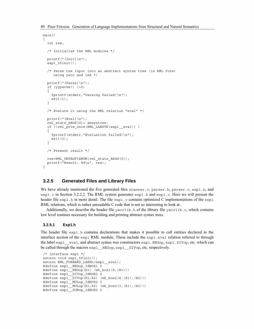
80 Peter Fritzson Generation of Language Implementations from Structural and Natural Semantics
main() { int res; /* Initialize the RML modules */ printf("[Init]\n"); exp1_5finit(); /* Parse the input into an abstract syntax tree (in RML form) using yacc and lex */ printf("[Parse]\n"); if (yyparse() !=0) { fprintf(stderr,"Parsing failed!\n"); exit(1); } /* Evalute it using the RML relation "eval" */ printf("[Eval]\n"); rml_state_ARGS[0]= absyntree; if (!rml_prim_once(RML_LABPTR(exp1__eval)) ) { fprintf(stderr,"Evaluation failed!\n"); exit(2); } /* Present result */ res=RML_UNTAGFIXNUM(rml_state_ARGS[0]); printf("Result: %d\n", res); }
3.2.5 Generated Files and Library Files
We have already mentioned the five generated files scanner.c, parser.h, parser.c, exp1.h, and exp1.c in Section 3.2.2.2. The RML system generates exp1.h and exp1.c. Here we will present the header file exp1.h in more detail. The file exp1.c contains optimized C implementations of the exp1 RML relations, which is rather unreadable C code that is not so interesting to look at.
Additionally, we describe the header file yacclib.h of the library file yacclib.c, which contains low level routines necessary for building and printing abstract syntax trees.
3.2.5.1 Exp1.h
The header file exp1.h contains declarations that makes it possible to call entities declared in the interface section of the exp1 RML module. These include the exp1.eval relation referred to through the label exp1__eval, and abstract syntax tree constructors exp1.NEGop, exp1.DIVop, etc. which can be called through the macros exp1__NEGop, exp1__DIVop, etc. respectively. /* interface exp1 */ extern void exp1_5finit(); extern RML_FORWARD_LABEL(exp1__eval); #define exp1__NEGop_3dBOX1 5 #define exp1__NEGop(X1) (mk_box1(5,(X1))) #define exp1__DIVop_3dBOX2 4 #define exp1__DIVop(X1,X2) (mk_box2(4,(X1),(X2))) #define exp1__MULop_3dBOX2 3 #define exp1__MULop(X1,X2) (mk_box2(3,(X1),(X2))) #define exp1__SUBop_3dBOX2 2

Chapter 3 Getting Started with the RML System 81
#define exp1__SUBop(X1,X2) (mk_box2(2,(X1),(X2))) #define exp1__ADDop_3dBOX2 1 #define exp1__ADDop(X1,X2) (mk_box2(1,(X1),(X2))) #define exp1__INTconst_3dBOX1 0 #define exp1__INTconst(X1) (mk_box1(0,(X1)))
3.2.5.2 Yacclib.h
The header file yacclib.h declares a number of primitive routines which are primarily used in the course of building abstract syntax trees during parsing.
The routines mk_icon, mk_rcon, mk_scon create RML representations for integers, real numbers and strings, respectively, whereas print_icon, print_rcon, and print_scon can print RML integers, real numbers and strings.
List construction is provided by mk_cons which creates a list cell and mk_nil which creates a nil pointer to represent the end of a list. The mk_none and mk_some constructors are used for the builtin RML option type which is convenient for representing optional syntactic constructs.
Finally, the routines mk_box0 to mk_box5 construct abstract syntax tree nodes of arity 0 to 5. These should not be called directly, however. Instead use the abstract syntax building routines, one for each node type, which are declared in the file exp1.h. /* yacclib.h */ extern int yylineno; /* generated by lex */ extern char *yytok2str(int token); /* uses yytoks[] from yacc + -DYYDEBUG * / extern void error(const char *fmt, ...); extern void *alloc_bytes(unsigned nbytes); extern void *alloc_words(unsigned nwords); extern void print_icon(FILE*, void*); extern void print_rcon(FILE*, void*); extern void print_scon(FILE*, void*); extern void *mk_icon(int); extern void *mk_rcon(double); extern void *mk_scon(char*); extern void *mk_nil(void); extern void *mk_cons(void*, void*); extern void *mk_none(void); extern void *mk_some(void*); extern void *mk_box0(unsigned ctor); extern void *mk_box1(unsigned ctor, void*); extern void *mk_box2(unsigned ctor, void*, void*); extern void *mk_box3(unsigned ctor, void*, void*, void*); extern void *mk_box4(unsigned ctor, void*, void*, void*, void*); extern void *mk_box5(unsigned ctor, void*, void*, void*, void*, void*);
3.3 An Evaluator for PAMDECL
3.3.1 Running the PAMDECL Evaluator
The executable is named pamdecl, and is invoked by typing pamdecl at the Unix prompt (sen20%10). Input typed by the user is shown in boldface. sen20%10 cat|pamdecl

82 Peter Fritzson Generation of Language Implementations from Structural and Natural Semantics
program a: integer; foo: real; body a:=17; foo:=a*2+8; write foo; end program ^D 42.0
Supplied with PAMDECL are a number of test programs located in subdirectory prg/. To run prg5 type the following: (??only for Unix) sen20%11 pamdecl > prg/prg5
1.01 1.0201 1.04060401 1.08285670562808 1.1725786449237 1.3749406785311 1.89046186947955 3.57384607995613 12.7723758032178 163.133583658624 26612.5661173053 708228675.347948
3.3.2 Building the PAMDECL Evaluator
The following files are needed for building PAMDECL: absyn.rml (page 55), env.rml (page 55), eval.rml (page 56), lexer.l, parser.y, main.rml, scanparse.rml, scanparse.c, yacclib.c, yacclib.h and makefile.
The files can be copied from /home/pelab/pub/pkg/rml/current/bookexamples/ examples/pamdecl (??update location) or typed from the above pages and Section 3.3.3 below.
The executable is built by typing: sen20%12 make pamdecl
3.3.3 Source Files for PAMDECL Evaluator
For absyn.rml, env.rml, and eval.rml see Section 2.8.
3.3.3.1 lexer.l %{ #include <stdlib.h> #include "parser.h" #include "rml.h" #include "yacclib.h" #include "absyn.h" typedef void *rml_t; extern rml_t yylval; int absyn_integer(char *s); int absyn_ident_or_keyword(char *s); %}

Chapter 3 Getting Started with the RML System 83
digit [0-9] digits {digit}+ letter [A-Za-z_] intcon {digits} dot "." sign [+-] exponent ([eE]{sign}?{digits}) realcondot {digits}{dot}{digits}{exponent}? realconexp {digits}({dot}{digits})?{exponent} realcon {realcondot}|{realconexp} ident {letter}({letter}|{digit})* ws [ \t\n] junk .|\n %% "(" return T_LPAREN; ")" return T_RPAREN; "+" return T_PLUS; "-" return T_MINUS; "*" return T_TIMES; "/" return T_DIVIDE; ":=" return T_ASSIGN; ";" return T_SEMICOLON; ":" return T_COLON; "<" return T_LT; "<=" return T_LE; ">" return T_GT; ">=" return T_GE; "<>" return T_NE; "=" return T_EQ; {intcon} { return absyn_integer(yytext);} {realcon} { return absyn_real(yytext);} {ident} { return absyn_ident_or_keyword(yytext); } {ws}+ ; {junk}+ return T_GARBAGE; %% /* Make an RML integer from a C string representation (decimal), box it for our abstract syntax, put in yylval and return constant token. */ int absyn_integer(char *s) { yylval=(rml_t) Absyn__INTCONST(mk_icon(atoi(s))); return T_CONST_INT; } /* Make an RML real from a C string representation, box it for our abstract syntax, put in yylval and return constant token. */ int absyn_real(char *s) { yylval=(rml_t) Absyn__REALCONST(mk_rcon(atof(s))); return T_CONST_REAL; } /* Make an RML Ident or a keyword token from a C string */

84 Peter Fritzson Generation of Language Implementations from Structural and Natural Semantics
static struct keyword_s { char *name; int token; } kw[] = { {"body", T_BODY}, {"do", T_DO}, {"else", T_ELSE}, {"end", T_END}, {"if", T_IF}, {"program", T_PROGRAM}, {"then", T_THEN}, {"while", T_WHILE}, {"write", T_WRITE}, }; int absyn_ident_or_keyword(char *s) { int low = 0; int high = (sizeof kw) / sizeof(struct keyword_s) - 1; while( low <= high ) { int mid = (low + high) / 2; int cmp = strcmp(kw[mid].name, yytext); if( cmp == 0 ) { return kw[mid].token; } else if( cmp < 0 ) low = mid + 1; else high = mid - 1; } yylval = (rml_t) mk_scon(s); return T_IDENT; }
3.3.3.2 parser.y %{ #include <stdio.h> #include "yacclib.h" #include "absyn.h" typedef void *rml_t; #define YYSTYPE rml_t extern rml_t absyntree; %} %token T_PROGRAM %token T_BODY %token T_END %token T_IF %token T_THEN %token T_ELSE %token T_WHILE %token T_DO %token T_WRITE %token T_ASSIGN %token T_SEMICOLON %token T_COLON

Chapter 3 Getting Started with the RML System 85
%token T_CONST_INT %token T_CONST_REAL %token T_CONST_BOOL %token T_IDENT %token T_LPAREN T_RPAREN %nonassoc T_LT T_LE T_GT T_GE T_NE T_EQ %left T_PLUS T_MINUS %left T_TIMES T_DIVIDE %left T_UMINUS %token T_GARBAGE %% program : T_PROGRAM decl_list T_BODY stmt_list T_END T_PROGRAM { absyntree = Absyn__PROG($2,$4); } decl_list : { $$ = mk_nil();} | decl decl_list { $$ = mk_cons($1,$2); } decl : T_IDENT T_COLON T_IDENT T_SEMICOLON { $$ = Absyn__NAMEDECL($1,$3);} stmt_list : { $$ = mk_nil();} | stmt stmt_list { $$ = mk_cons($1,$2); } stmt : simple_stmt T_SEMICOLON | combined_stmt simple_stmt : assign_stmt | write_stmt | noop_stmt combined_stmt : if_stmt | while_stmt assign_stmt : T_IDENT T_ASSIGN expr { $$ = Absyn__ASSIGN($1,$3);} write_stmt : T_WRITE expr { $$ = Absyn__WRITE($2);} noop_stmt : { $$ = Absyn__NOOP;} if_stmt : T_IF expr T_THEN stmt_list T_ELSE stmt_list T_END T_IF
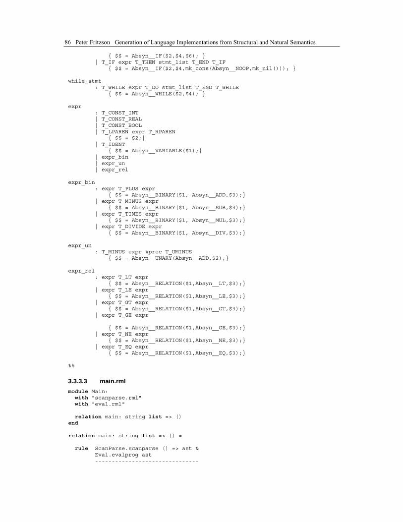
86 Peter Fritzson Generation of Language Implementations from Structural and Natural Semantics
{ $$ = Absyn__IF($2,$4,$6); } | T_IF expr T_THEN stmt_list T_END T_IF { $$ = Absyn__IF($2,$4,mk_cons(Absyn__NOOP,mk_nil())); } while_stmt : T_WHILE expr T_DO stmt_list T_END T_WHILE { $$ = Absyn__WHILE($2,$4); } expr : T_CONST_INT | T_CONST_REAL | T_CONST_BOOL | T_LPAREN expr T_RPAREN { $$ = $2;} | T_IDENT { $$ = Absyn__VARIABLE($1);} | expr_bin | expr_un | expr_rel expr_bin : expr T_PLUS expr { $$ = Absyn__BINARY($1, Absyn__ADD,$3);} | expr T_MINUS expr { $$ = Absyn__BINARY($1, Absyn__SUB,$3);} | expr T_TIMES expr { $$ = Absyn__BINARY($1, Absyn__MUL,$3);} | expr T_DIVIDE expr { $$ = Absyn__BINARY($1, Absyn__DIV,$3);} expr_un : T_MINUS expr %prec T_UMINUS { $$ = Absyn__UNARY(Absyn__ADD,$2);} expr_rel : expr T_LT expr { $$ = Absyn__RELATION($1,Absyn__LT,$3);} | expr T_LE expr { $$ = Absyn__RELATION($1,Absyn__LE,$3);} | expr T_GT expr { $$ = Absyn__RELATION($1,Absyn__GT,$3);} | expr T_GE expr { $$ = Absyn__RELATION($1,Absyn__GE,$3);} | expr T_NE expr { $$ = Absyn__RELATION($1,Absyn__NE,$3);} | expr T_EQ expr { $$ = Absyn__RELATION($1,Absyn__EQ,$3);} %%
3.3.3.3 main.rml module Main: with "scanparse.rml" with "eval.rml" relation main: string list => () end relation main: string list => () = rule ScanParse.scanparse () => ast & Eval.evalprog ast -------------------------------

Chapter 3 Getting Started with the RML System 87
main _ end
3.3.3.4 scanparse.rml module ScanParse: with "absyn.rml" relation scanparse: () => Absyn.Prog end
3.3.3.5 scanparse.c /* Glue to call parser (and thus scanner) from RML */ #include <stdio.h> #include "rml.h" /* Provide error reporting function for yacc */ yyerror(char *s) { extern int yylineno; fprintf(stderr,"Error: bad syntax on line %d.\n",yylineno); } /* The yacc parser will deposit the syntax tree here */ void *absyntree; /* No init for this module */ void ScanParse_5finit(void) {} /* The glue function */ RML_BEGIN_LABEL(ScanParse__scanparse) { if (yyparse() !=0) { fprintf(stderr,"Fatal: parsing failed!\n"); RML_TAILCALLK(rmlFC); } rmlA0=absyntree; RML_TAILCALLK(rmlSC); } RML_END_LABEL
3.3.3.6 makefile # Makefile for building PAMDECL # # ??Note: LDFLAGS, CFLAGS are non-portable for some Unix systems # VARIABLES SHELL = /bin/sh LDLIBS = -lrml -ll # Order is essential; we want librml main, not libll! LDFLAGS = -L$(RMLRUNTIME)/lib/plain/ CC = gcc CFLAGS = -I$(RMLRUNTIME)/include/plain/ -g -I.. # EVERYTHING all: pamdecl
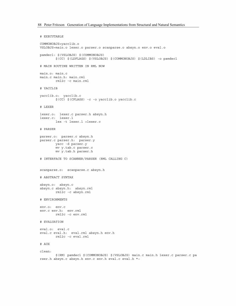
88 Peter Fritzson Generation of Language Implementations from Structural and Natural Semantics
# EXECUTABLE COMMONOBJS=yacclib.o VSLOBJS=main.o lexer.o parser.o scanparse.o absyn.o env.o eval.o pamdecl: $(VSLOBJS) $(COMMONOBJS) $(CC) $(LDFLAGS) $(VSLOBJS) $(COMMONOBJS) $(LDLIBS) -o pamdecl # MAIN ROUTINE WRITTEN IN RML NOW main.o: main.c main.c main.h: main.rml rml2c -c main.rml # YACCLIB yacclib.o: yacclib.c $(CC) $(CFLAGS) -c -o yacclib.o yacclib.c # LEXER lexer.o: lexer.c parser.h absyn.h lexer.c: lexer.l lex -t lexer.l >lexer.c # PARSER parser.o: parser.c absyn.h parser.c parser.h: parser.y yacc -d parser.y mv y.tab.c parser.c mv y.tab.h parser.h # INTERFACE TO SCANNER/PARSER (RML CALLING C) scanparse.o: scanparse.c absyn.h # ABSTRACT SYNTAX absyn.o: absyn.c absyn.c absyn.h: absyn.rml rml2c -c absyn.rml # ENVIRONMENTS env.o: env.c env.c env.h: env.rml rml2c -c env.rml # EVALUATION eval.o: eval.c eval.c eval.h: eval.rml absyn.h env.h rml2c -c eval.rml # AUX clean: $(RM) pamdecl $(COMMONOBJS) $(VSLOBJS) main.c main.h lexer.c parser.c pa rser.h absyn.c absyn.h env.c env.h eval.c eval.h *~
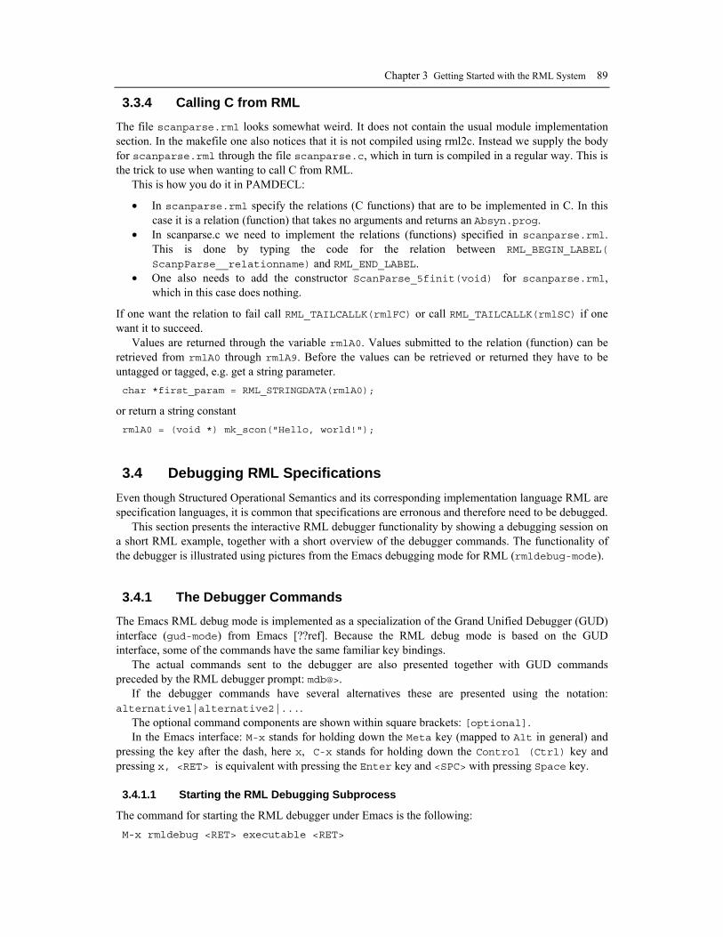
Chapter 3 Getting Started with the RML System 89
3.3.4 Calling C from RML
The file scanparse.rml looks somewhat weird. It does not contain the usual module implementation section. In the makefile one also notices that it is not compiled using rml2c. Instead we supply the body for scanparse.rml through the file scanparse.c, which in turn is compiled in a regular way. This is the trick to use when wanting to call C from RML.
This is how you do it in PAMDECL:
• In scanparse.rml specify the relations (C functions) that are to be implemented in C. In this case it is a relation (function) that takes no arguments and returns an Absyn.prog.
• In scanparse.c we need to implement the relations (functions) specified in scanparse.rml. This is done by typing the code for the relation between RML_BEGIN_LABEL(
ScanpParse__relationname) and RML_END_LABEL. • One also needs to add the constructor ScanParse_5finit(void) for scanparse.rml,
which in this case does nothing.
If one want the relation to fail call RML_TAILCALLK(rmlFC) or call RML_TAILCALLK(rmlSC) if one want it to succeed.
Values are returned through the variable rmlA0. Values submitted to the relation (function) can be retrieved from rmlA0 through rmlA9. Before the values can be retrieved or returned they have to be untagged or tagged, e.g. get a string parameter. char *first_param = RML_STRINGDATA(rmlA0);
or return a string constant rmlA0 = (void *) mk_scon("Hello, world!");
3.4 Debugging RML Specifications Even though Structured Operational Semantics and its corresponding implementation language RML are specification languages, it is common that specifications are erronous and therefore need to be debugged.
This section presents the interactive RML debugger functionality by showing a debugging session on a short RML example, together with a short overview of the debugger commands. The functionality of the debugger is illustrated using pictures from the Emacs debugging mode for RML (rmldebug-mode).
3.4.1 The Debugger Commands
The Emacs RML debug mode is implemented as a specialization of the Grand Unified Debugger (GUD) interface (gud-mode) from Emacs [??ref]. Because the RML debug mode is based on the GUD interface, some of the commands have the same familiar key bindings.
The actual commands sent to the debugger are also presented together with GUD commands preceded by the RML debugger prompt: mdb@>.
If the debugger commands have several alternatives these are presented using the notation: alternative1|alternative2|....
The optional command components are shown within square brackets: [optional]. In the Emacs interface: M-x stands for holding down the Meta key (mapped to Alt in general) and
pressing the key after the dash, here x, C-x stands for holding down the Control (Ctrl) key and pressing x, <RET> is equivalent with pressing the Enter key and <SPC> with pressing Space key.
3.4.1.1 Starting the RML Debugging Subprocess
The command for starting the RML debugger under Emacs is the following: M-x rmldebug <RET> executable <RET>

90 Peter Fritzson Generation of Language Implementations from Structural and Natural Semantics
3.4.1.2 Setting/Deleting Breakpoints
A part of a session using this type of commands is shown in Figure 3-1. The presentation of the commands follows later.
Figure 3-1. Using breakpoints.
To set a breakpoint on the line the cursor (point) is at: C-x <SPC> mdb@> break on file:lineno|string <RET>
To delete a breakpoint placed on the current source code line (gud-remove): C-c C-d C-x C-a C-d mdb@> break off file:lineno|string <RET>
Instead of writing break one can use alternatives: br|break|breakpoint. Alternatively one can delete all breakpoints using:
mdb@> cl|clear <RET>
Showing all breakpoints: mdb@> sh|show <RET>
3.4.1.3 Stepping and Running
To perform one step (gud-step) in the RML code:

Chapter 3 Getting Started with the RML System 91
C-c C-s C-x C-a C-s mdb@> st|step <RET>
To continue after a step or a breakpoint (gud-cont) in the RML code: C-c C-r C-x C-a C-r mdb@> ru|run <RET>
Examples of using these commands are shown in Figure 3-2. The example is the Exp1 calculator briefly described in Section 2.1.
Figure 3-2. Stepping and running in the debugger.
3.4.1.4 Examining Data
There are no GUD keybindings for these commands but they are inspired from the GNU Project debugger (GDB) [ref??].
To print the contents/size of a variable one can write: mdb@> pr|print variable_name <RET> mdb@> sz|sizeof variable_name <RET>
at the debugger prompt. The size is displayed in bytes. Variable values to be printed can be of a complex type and very large. One can restrict the depth of
printing using: mdb@> [set] de|depth integer <RET>
Moreover, we have implemented an external viewer written in Java called RMLDataViewer to browse the contents of such a large variable. To send the contents of a variable to the external viewer for inspection one can use the command: mdb@> bw|browse|gr|graph var_name <RET>

92 Peter Fritzson Generation of Language Implementations from Structural and Natural Semantics
at the debugger prompt. The debugger will try to connect to the RMLDataViewer and send the contents of the variable. The external data browser has to be started a priori. If the debugger cannot connect to the external viewer within a specified timeout a warning message will be displayed. A picture with the external RMLDataViewer tool is presented in Figure 3-3:
Figure 3-3. External browser/viewer for complicated data structures.
If the variable which one tries to print does not exist in the current scope (not a live variable) a notifying warning message will be displayed.
Automatic printing of variables at every step or breakpoint can be specified by adding a variable to a display list: mdb@> di|display variable_name <RET>
To print the entire display list: mdb@> di|display <RET>
Removing a display variable from the display list: mdb@> un|undisplay variable_name <RET>
Removing all variables from the display list: mdb@> undisplay <RET>
Printing the current live variables: mdb@> li|live|livevars <RET>
Instructing the debugger to print or to disable the print of the live variable names at each step/breapoint: mdb@> [set] li|live|livevars [on|off]<RET>
Figure 3-4 shows examples of some of these data examination commands within a debugging session:

Chapter 3 Getting Started with the RML System 93
Figure 3-4. Examining data in the debugger command window.
3.4.1.5 Additional commands
The stack contents (backtrace) can be displayed using: mdb@> bt|backtrace <RET>
Because the contents of the stack can be quite large, one can print a filtered view of it: mdb@> fbt|fbacktrace filter_string <RET>
Also, one can restrict the numbers of entries the debugger is storing using: mdb@> maxbt|maxbacktrace integer <RET>
For displaying the status of the RML runtime: mdb@> sts|stat|status <RET>
The status of the extended RML runtime comprises information regarding the garbage collector, allocated memory, stack usage, etc.
The current debugging settings can be displayed using: mdb@> stg|settings <RET>
The settings printed are: the maximum remembered backtrace entries, the depth of variable printing, the current breakpoints, the live variables, the list of the display variables and the status of the runtime system.
One can invoke the debugging help by issuing: mdb@> he|help <RET>
For leaving the debugger one can use the command: mdb@> qu|quit|ex|exit|by|bye <RET>

94 Peter Fritzson Generation of Language Implementations from Structural and Natural Semantics
A session using these commands is presented in Figure 3-5 below:
Figure 3-5. Additional debugger commands.
(BRK)

95
Chapter 4 Declarative Programming in RML
The focus of this chapter is a more comprehensive overview of declarative programming facilities available in RML which are useful not only for language specification, but also for declarative programming in general. A short introduction to this topic, including a factorial example, was earlier given in Section 2.4.2. Now we continue with a more complete presentation, starting with the RML module concept, following by RML typing and type declaration facilities, RML rules and relations, and finally some special issues. (?? also programming styles, binary lookup, etc.)
4.1 Modules The complexity of a large specifications—as for any large pieces of software—requires modularization and information hiding. Therefore RML provides a simple module system. Relations and type definitions which describe the same or related language properties should be placed in the same module. The general structure of a module is as follows: module modulename: with "import_module_name1" with "import_module_name2" ... <exported_type_declarations> ... <exported_relation_signatures> ... end (* of interface section *) (* Start of implementation section *) with "import_module_name3" with "import_module_name4" ... relation rel_name1: ... ... relation rel_name2: ... ...
A module consists of an interface section and an optional implementation section:
• The mandatory interface section is used to specify the name of the declared module itself preceded by the keyword module and followed by a colon, the set of imported other modules are used in the interface section as specified by with-statements, and which types and relations declared in the module that are exported to other modules.
• Then follows an optional implementation section. It starts with an optional list of with-statements, specifying which additional modules are used in this section. The rest of the implementation section consists of complete relation declarations.
Several examples of RML modules are presented in detail in Section 2.7.4.

96 Peter Fritzson Generation of Language Implementations from Structural and Natural Semantics
4.2 Global Constant Variables Global variables can be declared in RML through the val keyword, e.g. as below where the init_env variable is initialized to the empty list: val init_env = []
Such variables are single-assignment—they can only be assigned once—according to the declarative nature of Structured Operational Semantics and RML. Therefore such variables are actually constants.
4.3 Types The RML language supports a builtin set of primitive data types as well as means of declaring more complex types and structures such as tuples and tree structures. First we will take a look at the primitive data types.
4.3.1 Primitive Data Types
The RML language provides a basic set of primitive types found in most programming languages:
• char—8-bit characters, e.g. #"A" (the character A). • bool—booleans, e.g. true/false. • int—integers, e.g. -123. (?? 31-bit integers in RML; Long integers are also available ?) • real—double-precision IEEE floating point numbers, e.g. 3.2E5. (?? single-prec float?) • string—strings of characters, e.g. "Linköping".
A number of builtin primitive operations are provided on values of those types as builtin RML relations. Below we just mention the names of those builtin relations. Their type signatures and semantics are specified in Appendix B??.
Boolean operations: bool_and, bool_or, bool_not
Integer operations: int_add, int_sub, int_mul, int_div
int_mod, int_abs, int_neg, int_max, int_min
int_lt, int_le, int_eq, int_ne, int_ge, int_gt, int_real, int_string
Real number operations: real_add, real_sub, real_mul, real_div
real_mod, real_abs, real_neg, real_max, real_min
real_lt, real_le, real_eq, real_ne, real_ge, real_gt, real_int, real_string
real_cos, real_sin, real_atan, real_exp, real_ln, real_floor, real_int, real_pow
String operations: string_length, string_nth, string_append
string_int, string_list, list_string
There is also a generic equality operator, =, which can be applied to values of primitive data types as well as to values of structured types such as arrays, lists, and trees.
Chapter 4 Declarative Programming in RML 97
4.3.2 Type Name Declarations
Alternate names for types in RML can be introduced through the type declaration, e.g.: type Identifier = string type IntConstant = int type MyValue = real
4.3.3 Tuples
Tuples are represented by parenthesized, comma-separated sequences of items each of which may have a different type, e.g.:
• (55,66)— a 2-tuple of integers. • (55,"Hello",INTconst(77))— a 3-tuple of integer, string, and Exp.
Tuple types are specified by constituent types separated by an asterix (*). Named tuple types can be declared explicitly through the type declaration: type TwoInt = int * int type Threetuple = int * string * Exp
For the case where several variants of a tuple type are needed within approximately the same “type”, e.g. of two numbers such as (35,37) with the type int * int, and two other numbers (33,44.5) with the type int * real, it is recommended to switch to using tagged union types (see below) for which each variant is tagged to provide unambiguous type information.
4.3.4 Tagged Union Types for Records, Trees, and Graphs
The datatype declaration in RML is used to introduce union types, for example the type Number below, which can be used to represent several kinds of number types such as integers, rational numbers, real, and complex within the same type: datatype Number = INT of int | RATIONAL of int * int | REAL of real | COMPLEX of real * real
The different names, INT, RATIONAL, REAL and COMPLEX, are called constructors, as they are used to construct tagged instances of the type. For example, we can construct a Number instance REAL(3.14) to hold a real number or another instance COMPLEX(2.1,3.5) to hold a complex number.
Each variant of such a union type is actually a kind of record type with one or more unnamed fields that can only be referred to by their position in the record. The type Number can be viewed as the union of the record types INT, RATIONAL, REAL and COMPLEX.
When declaring union types consisting of more than one field (e.g. COMPLEX above which has two real-valued fields) the special symbol * is used to separate the field types.
The most frequent use of union types in RML is to specify abstract syntax tree representations used in language specifications as we have seen many examples of in earlier chapters of this book, e.g. Exp below, first presented in Section 2.1.2: datatype Exp = INTconst of int | ADDop of Exp * Exp | SUBop of Exp * Exp | MULop of Exp * Exp | DIVop of Exp * Exp | NEGop of Exp
The constructors INTconst, ADDop, SUBop, etc. are can be used to construct nodes in abstract syntax trees such as INTconst(55) and ADDop(INTconst(6),INTconst(44)), etc.

98 Peter Fritzson Generation of Language Implementations from Structural and Natural Semantics
Representing DAG (Directed Acyclic Graph) structures is no problem. Just pass the same argument twice or more and the child node will be shared, e.g. when building an addition node using the ADDop constructor below: ADDop(x, x)
However, building circular structures is not possible because of the declarative side-effect free nature of RML. Once a node has been constructed it cannot be modified to point to itself. Recursive dependencies such as recursive types have to be represented with the aid of some intermediate node. An example of this technique is the representation of recursive record type references in the Petrol language using UNFOLD nodes, see Section 6.6.2.
4.3.5 Parameterized Data Types
A parameterized data type in RML is a type that may have another type as a parameter. A parameterized type available in most programming languages is the array type which is usually parameterized in terms of its array element type. For example, we can have integer arrays, string arrays, or real arrays, etc. depending on the type of the array elements. The size of an array may also be regarded as a parameter of the array.
The RML language provides three kinds of parameterized types:
• Lists – the list keyword, parameterized in terms of the list element type. • Vectors – the vector keyword, parameterized in terms of the vector element type. • Option types – the option keyword, parameterized in terms of the type of the optional value.
Note that all parameterized types in RML are monomorphic: all elements have to have the same type, i.e., you cannot mix elements of type real and type string within the same array or list. Certain languages provide polymorphic arrays, i.e., array elements may have different types.
However, arrays of elements of “different” types in RML can be represented by arrays of elements of tagged union types, where each “type” in the union type is denoted by a different tag.
4.3.5.1 Lists
Lists are common data structures in declarative languages since they conveniently allow representation and manipulation of sequences of elements. Elements can be efficiently (in constant time) added to beginning of lists in a declarative way. The following basic list construction operators are available:
• The list constructor: [el1,el2,el3,...]creates a list of elements el1, el2, ... of identical type. Examples:[] denotes the empty list; [2,3,4] is a list of integers, etc.
• The empty list is denoted by nil or []. (?? nil is not needed in RML since we have [] ?) • The list element concatenation operation cons(element, lst) or using the equivalent ::
operator syntax as in element :: lst, adds an element in front of the list lst and returns the resulting list. For example: cons("a", ["b"]) => ["a", "b"]; cons("a",[]) => ["a"] "a"::"b"::"c"::[] => ["a","b","c"];
Additional builtin RML list operations are briefly described by the following examples; see Appendix ??B for type signatures of these relations:
• list_append([2,3],[4,5]) => [2,3,4,5] • list_reverse([2,3,4,5]) => [5,4,3,2]
• list_length([2,3,4,5]) => 4
• list_member(3, [2,3,4,5]) => true
• list_nth([2,3,4,5], 4) => 5 (?? current list_nth start indexing at zero?)

Chapter 4 Declarative Programming in RML 99
• list_delete([2,3,4,5],2) => [2,4,5] (?? current list_delete starts indexing at zero?)
The most readable and convenient way of accessing elements in an existing list or constructing new lists is through pattern matching operations, see Section 4.5.2.
The types of lists often need to be specified. Named list types can be declared using RML type declarations: type IntegerList = int list
An example of a list type for lists of real elements: type RealList = real list;
The following is a parameterized RML list type with an unspecified element type 'elemtype which is a type parameter (type variable) of the list. Type variable names in RML start by a single quote ('). 'elemtype list;
Lists in the RML language are monomorphic, i.e., all elements must have the same type. Lists of elements with “different” types can be represented by lists of elements of tagged union types, where each type in the union type has a different tag.
4.3.5.2 Vectors
An RML vector is a sequence of elements, all of the same type. The main advantage of a vector compared to a list is that an arbitrary element of a vector can be accessed in constant time by a vector indexing operation on a vector and an integer denoting the ordinal position of the element.
Constructing vectors is rather clumsy in RML. First a list has to be constructed which then is converted to a vector, e.g.: list_vector([2,4,6,8]) => vec
Accessing the third element of the vector vec using the vector indexing operation vector_nth, where the first element has index 1: vector_nth(vec,3) => 6 (?? update vector_nth to start indexing by 1)
Getting the length of vector vec: vector_length(vec) => 4
Named array types can of course be declared using the type construct, e.g. as in the declaration of a one-dimensional vector of boolean values: type OneDimBooleanVector = bool vector
Multi-dimensional arrays are represented by arrays of arrays, e.g. as in the following declaration of a two-dimensional matrix of real elements. type TwoDimRealMatrix = real vector vector
Parameterized vector types can be expressed using a type parameter such as 'elemtype in the following example, again noting that type parameter names in RML start by a single quote ('): 'elemtype vector
Below we give the type signatures, i.e. the types of input parameters and output results, for a few builtin vector operations, also presented in Appendix B??. The following are the length and indexing signatures: relation vector_length: 'a vector => int // length of vector relation vector_nth: ('a vector, int) => 'a // extracts vector element
These are the conversion operations between vectors and lists: relation vector_list: 'a vector => 'a list // convert to list relation list_vector: 'a list => 'a vector // convert to vector

100 Peter Fritzson Generation of Language Implementations from Structural and Natural Semantics
4.3.5.3 Option Types
Option types have been introduced in RML to provide a type-safe way of representing the common situation where a data item is optionally present in a data structure – which in language specification applications typically is an abstract syntax tree.
The option type can be viewed as a predefined parameterized RML union type, that works as if it was a parameterized datatype declaration of the following form (not allowed in RML): datatype ’atype option = NONE | SOME of ’atype
The constructor NONE is used to represent the case where the optional data item (of type 'atype in the above example) is not present, whereas the constructor SOME is used when the data item is present in the data structure.
One example of use of the option type is the function or procedure declaration in the Petrol language, where the function/procedure body is optionally present since it is not present for external functions/procedures (Section 6.5 and Section 6.10.1.2). Another example is the optional return value in return statements (Section 6.10.8). A third example is its use in binary search trees (Section ??).
4.4 RML Relations We have already used RML relations extensively to express the semantics of a number of small languages, as well as small declarative programs. This section gives a more complete presentation of the RML relation construct, its properties, and its usage.
4.4.1 Builtin Relations
A number of “standard” builtin primitives are provided by the RML standard library—in a module called rml. Examples are int_add, int_sub, string_append, list_append, etc. A complete list of these primitives can be found in ??Appendix B. (?? Note: arithmetic operators +,-,*, / will soon be supported)
4.4.2 RML Relations Versus Functions
Superficially, it may appear that the notion of RML relation is rather close to the notion of function in other specification languages. Both functions and RML relations maps input arguments to output results, whereas the most general form of relation maps both ways, e.g. as available in relational data bases or many logic programming languages.
The design “restriction” on RML relations to map input arguments to output results and not vice versa is motivated by the following:
• The great majority of language specifications are written in a style of mapping inputs to outputs. • Input to output mapping usually gives easier-to-understand specifications. • Input to output mapping allows generation of more efficient code from the specifications.
Typically, formal parameters are either transmitting input data to a relation, or producing output results. If a formal parameter is used for both purposes, this usually makes the specification harder to understand as well as causing problems of providing efficient implementations. Instead of having the same parameter for both purposes, separate input and output parameters can usually be provided with no loss of generality.
Two important properties of RML relations are however absent for functions:
• Relations can fail or succeed.

Chapter 4 Declarative Programming in RML 101
• Local backtracking is supported between rules in a relation.
A call to a relation can fail instead of always returning a result which is the case for functions. This is convenient for the specification writer when expressing semantics, since other possibly matching rules in the relation will be applied without needing “try-again” mechanisms to be directly encoded into specifications. The failure handling mechanism can also be used in general declarative programming, e.g. the factorial example previously presented in Section 2.4.2.1.
This brings us into the topic of backtracking. If there is a failure in rule, or in one of the relations directly or indirectly called via the premises of the rule, RML will backtrack (i.e., undo) the part of the “execution” which started from this rule, and automatically try the next rule (if there is one) in top-down, left-to-right order. If no rule in the relation matches and succeeds, then the call to this relation will fail. Correct back-tracking is however dependent on avoidance of side-effects in the rules of the specification.
4.4.3 Argument Passing and Result Values
Any kind of data structure, as well as relations, can be passed as actual arguments in a call to an RML relation. One or more results can be returned from such a call. The issues are discussed in some detail in the following sections.
4.4.3.1 Multiple Arguments and Results
An RML relation may be specified with multiple arguments, multiple results, or both. The syntax is simple, the argument and result types are just listed, separated by commas, enclosed by parenthesis, as in the signature of the example relation Multiple below: relation Multiple: (argtype1, argtype2, argtype3) => (restype1, restype2) = ...
Since relations can yield multiple results, propositions—which are part of axioms and rules—must of course also be able to accept multiple arguments and give multiple results. The syntax is the same as for the signature—the => arrow, e.g. in the proposition below containing a call to eval with three arguments and two results: eval(env, state, exp) => (value, state2)
4.4.3.2 Tuple Arguments and Results from Relations
We just noted that an RML relation can have multiple arguments and results. This should not be confused with the case where an RML tuple type (see Section 4.3.3) consisting of several constituent types is part of the signature of a relation. For example, the relation incrementpair below accepts a single tuple of two integers and returns a tuple where both integers have been incremented by one. An extra level of parentheses is needed for the tuple result to differ from the case of two result values. relation incrementpair: (int * int) => int * int =
axiom incrementpair((v1,v2)) => ((v1+1,v2+1)) end (*incrementpair *)
For example, the call: incrementpair((2,3))
gives the result: (3,4)

102 Peter Fritzson Generation of Language Implementations from Structural and Natural Semantics
4.4.3.3 Passing Relations as Arguments – Function Parameters
Relations can be passed as parameters, i.e., as a kind of function parameters. In the example below, the relation add1 is passed as a parameter to the relation map, which applies its formal parameter func to each element of the parameter list.
For example, applying the function add1 to each element in the list [0,1,2], e.g. map(add1, [0,1,2]), will give the result list [1,2,3]. relation add1: int => int =
rule int_add(x,1) => y ----------------- add1(x) => y end relation map 'elemtype list => 'elemtype list =
axiom map(func,[]) => [] rule F(x) => y & map(func,xs) => ys --------------------- map(func, x::xs) => y::ys end relation ... ... map(add1, [0,1,2]) => zs (* Pass add1 as a parameter to map *) (* In this example zs will be [1,2,3] *) ... end
4.5 Variables and Types in Relations Except for global constants, RML variables only occur in relations. Types, including parameterized types, can be explicitly declared in RML relation type signatures.
4.5.1.1 Type Variables and Parameterized Types in Relations
We have already presented the notion of parameterized list, vector, and option types in Section 4.3.5. Type variables in RML start with a single quote (') and can only appear in relation signatures.
For example, the tuple2_get_field1 relation takes a tuple of two values having arbitrary types specified by the type variables 'atype and 'btype, which in the example below will be bound to the types string and int, and returns the first value, e.g.: tuple2_get_field1(("x",33)) => "x"
The relation is parameterized in terms of the types of the first and second fields in the argument tuple, which is apparent from the type signature in its definition: relation tuple2_get_field1 : ('atype * 'btype) => 'atype =
axiom tuple2_get_field1((field1,_)) => field1
end
4.5.1.2 Local Variables in Relations
Variables in RML relations are normally introduced in rules and have a scope throughout the rule. The only exception are global constants. There are three kinds of local variables for values, as well as type variables which are introduced in relation signatures and include one or more apostrophes ('):
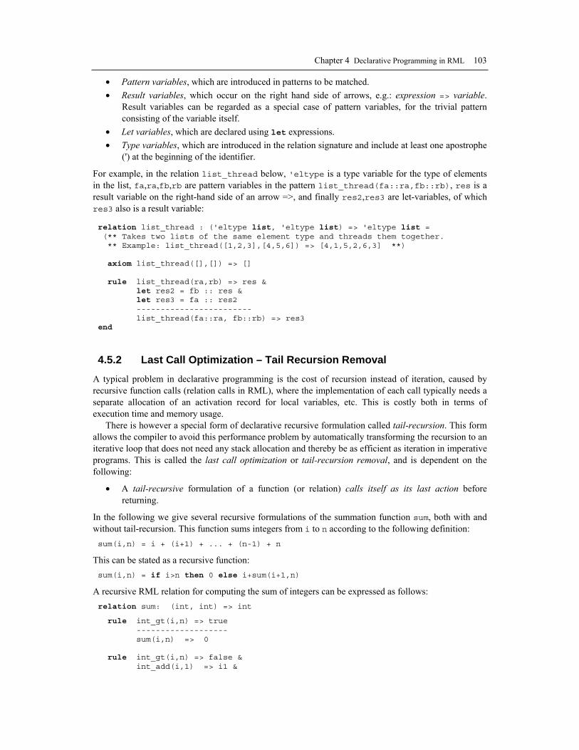
Chapter 4 Declarative Programming in RML 103
• Pattern variables, which are introduced in patterns to be matched. • Result variables, which occur on the right hand side of arrows, e.g.: expression => variable.
Result variables can be regarded as a special case of pattern variables, for the trivial pattern consisting of the variable itself.
• Let variables, which are declared using let expressions. • Type variables, which are introduced in the relation signature and include at least one apostrophe
(') at the beginning of the identifier.
For example, in the relation list_thread below, 'eltype is a type variable for the type of elements in the list, fa,ra,fb,rb are pattern variables in the pattern list_thread(fa::ra,fb::rb), res is a result variable on the right-hand side of an arrow =>, and finally res2,res3 are let-variables, of which res3 also is a result variable: relation list_thread : ('eltype list, 'eltype list) => 'eltype list = (** Takes two lists of the same element type and threads them together. ** Example: list_thread([1,2,3],[4,5,6]) => [4,1,5,2,6,3] **) axiom list_thread([],[]) => [] rule list_thread(ra,rb) => res & let res2 = fb :: res & let res3 = fa :: res2 ------------------------ list_thread(fa::ra, fb::rb) => res3 end
4.5.2 Last Call Optimization – Tail Recursion Removal
A typical problem in declarative programming is the cost of recursion instead of iteration, caused by recursive function calls (relation calls in RML), where the implementation of each call typically needs a separate allocation of an activation record for local variables, etc. This is costly both in terms of execution time and memory usage.
There is however a special form of declarative recursive formulation called tail-recursion. This form allows the compiler to avoid this performance problem by automatically transforming the recursion to an iterative loop that does not need any stack allocation and thereby be as efficient as iteration in imperative programs. This is called the last call optimization or tail-recursion removal, and is dependent on the following:
• A tail-recursive formulation of a function (or relation) calls itself as its last action before returning.
In the following we give several recursive formulations of the summation function sum, both with and without tail-recursion. This function sums integers from i to n according to the following definition: sum(i,n) = i + (i+1) + ... + (n-1) + n
This can be stated as a recursive function: sum(i,n) = if i>n then 0 else i+sum(i+1,n)
A recursive RML relation for computing the sum of integers can be expressed as follows: relation sum: (int, int) => int
rule int_gt(i,n) => true ------------------- sum(i,n) => 0 rule int_gt(i,n) => false & int_add(i,1) => i1 &

104 Peter Fritzson Generation of Language Implementations from Structural and Natural Semantics
sum(i1,n) => res1 & int_add(i,res1) => res2 -------------------- sum(i,n) => res2 end
The above relation sum is recursive but not tail-recursive since its last action is adding the result res1 of the sum call to i, i.e., the recursive call to sum is not the last action that occurs before returning from the relation.
Fortunately, it is possible to reformulate the function into tail-recursive form using the method of accumulating parameters, which we will show in the next section.
4.5.2.1 The Method of Accumulating Parameters for Collecting Results
The method of accumulating parameters is a general method for expressing declarative recursive computations in a way that allows collecting intermediate results during the computation and makes it easier to achieve an efficient tail-recursive formulation.
We reformulate the sum relation by adding an accumulating input parameter sumSoFar to a help function sumTail, keeping the counter i. When the terminating condition i>n occurs the accumulated sum sumSoFar is returned. The function sumTail is tail-recursive since the call to sumTail is the last action that occurs before returning from the function body, i.e.: sum(i,n) = sumTail(i,j,0)
sumTail(i,n,sumSoFar) = if i>n then sumSoFar else sumTail(i+1,n,i+sumSoFar)
The functions sum and sumTail expressed as RML relations: relation sum: (int,int) => int
axiom sumTail(i,n,0) => res ------------------- sum(i,n) => res end relation sumTail: (int,int,int) => int
rule int_gt(i,n) => true ------------------- sumTail(i,n,_) => 0 rule int_gt(i,n) => false & int_add(i,1) => i1 & int_add(i,sumSoFar) => res1 & sumTail(i1,n,res1) => res2 -------------------------- sumTail(i,n,sumSoFar) => res2 end
It is easy to see that the relation sumTail is tail-recursive since the call to sumTail is the last computation in the last premise of the second rule.
Another example of a tail-recursive formulation is a revised version of the previous list_thread relation from Section 4.5.1.2, called list_thread_tail: list_thread(a,b) = list_thread_tail(a,b,[])
We have introduced an accumulating parameter as the third argument of list_thread_tail, e.g.: list_thread_tail([1,2,3],[4,5,6],[]) => [4,1,5,2,6,3]
Its definition follows below: relation list_thread_tail : ('eltype list, 'eltype list, 'eltype list) => 'eltype list =

Chapter 4 Declarative Programming in RML 105
axiom list_thread_tail([],[],[]) => [] rule list_thread_tail(rest_a, rest_b, fa::fb::acclst) => res -------------------------------------------------- list_thread_tail(fa::rest_a, fb::rest_b, acclst) => res end
4.5.3 Relation Failure Versus Boolean Negation
We have previously mentioned that RML relations can fail or succeed, whereas conventional functions always succeed in returning some value. The most common cause for an RML relation to fail is the absence of a rule that matches and/or have premises that succeed. Another cause of failure is the use of the builtin RML command fail, which causes a relation to fail immediately.
It is important to note that fail is quite different from the logical value false. A relation returning false would still succeed since it returns a value. The builtin relation bool_not operates on the logical values true and false according to the following definition: relation bool_not: bool => bool = axiom bool_not(false) => true axiom bool_not(true) => false end
However, failure can in a logical sense be regarded as negation—similar to negation by failure in the Prolog programming language. A premise that fails will certainly cause the containing rule to fail. The RML not operator can however invert the logical sense of a proposition. The following premise is logically “true” since it succeeds (but it does not return the predefined value true): not relation_that_fails(x)
The two operators bool_not and not thus represent different forms of “negation”—negating the boolean value true, or negating the failure of a call to a relation.
4.5.4 Using Side Effects
Can side effects such as updating of global data or input/output be used in specifications? Consider the following contrived example: relation foo =
rule print "A" & condition_A(x) => y ----------------------------------- foo(x) => y rule print "B" & condition_B(x) => y ---------------------------------- foo(x) => y end
The builtin relation print is called in both rules, giving rise to the side effect of updating the output stream. The intent is that if condition_A is fulfilled, "A" should be printed and a value returned. On the other hand, if condition_B is fulfilled, "B" should be printed and some other value returned. The problem occurs if condition_A fails. Then backtracking will occur, and the next rule (which has the same matching pattern) will be tried. However, the printing of "A" has already occurred and cannot be undone.
Such problems can be avoided if the code is completely determinate—at most one rule in a relation matches and backtracking never occurs. Thus we may formulate the following usage rule:

106 Peter Fritzson Generation of Language Implementations from Structural and Natural Semantics
• Only use side-effects in completely deterministic relations for which at most one rule matches and backtracking may never occur.
The problem can be avoided by separating the print side effect from the locally non-determinate choice, which is put into a side-effect free relation choose_foo. relation choose_foo =
rule condition_A(x) => y ------------------------ choose_foo(x) => ("A",y) rule condition_B(x) => y ------------------------ choose_foo(x) => ("B",y) end relation foo(x)
rule choose_foo(x) => (z,y) & print z ---------------------------------- foo(x) => y end
In the above contrived example, the problem can also be avoided in an even simpler way by just putting print after the condition. (??Explain: why exactly is this possible?) relation foo’ =
rule condition_A(x) & print "A" => y ----------------------------------- foo(x) => y rule condition_B(x) & print "B" => y ---------------------------------- foo(x) => y end
A natural question concerns the circumstances when side effects may occur, since RML is basically a side-effect free specification language. The following two cases can however give rise to side effects:
• The print primitive causes side effects by updating the output stream. • External C functions which may contain side effects can be called from RML. • The tick primitive updates a counter internal to tick, to return a unique integer at each call.
As just noted, the builtin relation tick generates a new unique (integer) “identifier” at each call— analogous to a random number generator. In order to ensure that each new integer is unique, some global state (e.g. a counter) has to be updated, which is a side effect. However, from the point of view of a semantics specification the actual value from tick is irrelevant—only the uniqueness is important. It does not matter if tick is called a few extra times and some values are thrown away during backtracking. Thus, from a practical semantics point of view tick may be treated as a side effect free primitive if used in an appropriate way.
4.6 Pattern-Matching Pattern-matching on instances of structured data types is one of the central facilities provided by RML, which significantly contributes to the elegance and ease with which many language aspects may be specified. The pattern matching in RML is essentially identical to that of Standard ML, and very close to similar facilities in many functional languages.
Patterns can occur both on the left- and right-hand side of the arrow => in propositions in matching or constructive contexts, with somewhat different meanings.
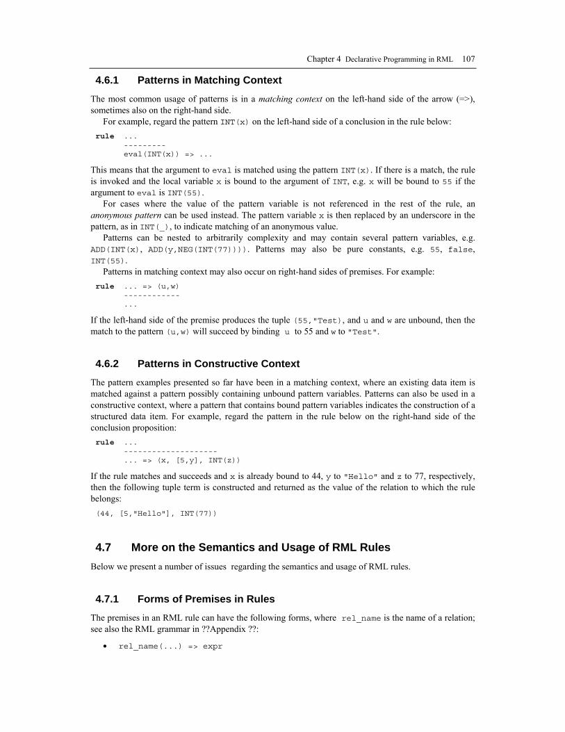
Chapter 4 Declarative Programming in RML 107
4.6.1 Patterns in Matching Context
The most common usage of patterns is in a matching context on the left-hand side of the arrow (=>), sometimes also on the right-hand side.
For example, regard the pattern INT(x) on the left-hand side of a conclusion in the rule below: rule ... --------- eval(INT(x)) => ...
This means that the argument to eval is matched using the pattern INT(x). If there is a match, the rule is invoked and the local variable x is bound to the argument of INT, e.g. x will be bound to 55 if the argument to eval is INT(55).
For cases where the value of the pattern variable is not referenced in the rest of the rule, an anonymous pattern can be used instead. The pattern variable x is then replaced by an underscore in the pattern, as in INT(_), to indicate matching of an anonymous value.
Patterns can be nested to arbitrarily complexity and may contain several pattern variables, e.g. ADD(INT(x), ADD(y,NEG(INT(77)))). Patterns may also be pure constants, e.g. 55, false, INT(55).
Patterns in matching context may also occur on right-hand sides of premises. For example: rule ... => (u,w) ------------ ...
If the left-hand side of the premise produces the tuple (55,"Test), and u and w are unbound, then the match to the pattern (u,w) will succeed by binding u to 55 and w to "Test".
4.6.2 Patterns in Constructive Context
The pattern examples presented so far have been in a matching context, where an existing data item is matched against a pattern possibly containing unbound pattern variables. Patterns can also be used in a constructive context, where a pattern that contains bound pattern variables indicates the construction of a structured data item. For example, regard the pattern in the rule below on the right-hand side of the conclusion proposition: rule ... -------------------- ... => (x, [5,y], INT(z))
If the rule matches and succeeds and x is already bound to 44, y to "Hello" and z to 77, respectively, then the following tuple term is constructed and returned as the value of the relation to which the rule belongs: (44, [5,"Hello"], INT(77))
4.7 More on the Semantics and Usage of RML Rules Below we present a number of issues regarding the semantics and usage of RML rules.
4.7.1 Forms of Premises in Rules
The premises in an RML rule can have the following forms, where rel_name is the name of a relation; see also the RML grammar in ??Appendix ??:
• rel_name(...) => expr

108 Peter Fritzson Generation of Language Implementations from Structural and Natural Semantics
• rel_name(...)
• var = expr
• not var = expr
• not rel_name(...)
• not rel_name(...) => expr
The not operator succeeds if the premise it operates on fails. The equality operator (=) succeeds if the data values are identical. Each of these forms can also be parenthesized.
4.7.2 Right Hand Sides of Rules
What can appear in a right-hand side of a rule? Calls to other RML relations are forbidden, whether builtin or user-defined. The reason is that the right hand side represents the result of a proposition, which is an instance of some data structure, or a variable or pattern which represents a possible data instance. Invocations of other RML relations may only occur on the left-hand side of propositions. Thus the following right-hand side is illegal: (?? motivate why; might be changed in future RML versions?) .... => int_real(x)
since it refers to the builtin relation int_real for conversion from integer to real. Variables and data type constructors are however allowed, as below: .... => ASSIGN(x,y)
where the right hand side is a pattern of a data item—an abstract syntax tree node—with the constructor ASSIGN from some abstract syntax type declaration defined as an RML union type.
4.7.3 Deterministic Rule Search
(*?? Discuss the difference between determinate and deterministic specifications/search?)
We remarked earlier that RML has been designed to be a determinate meta-language for Structured Operational Semantics. Thus, RML implements deterministic search of the set of rules within a relation, starting from the first rule and proceeding top-down, left-to-right, until some rule matches or there are no more rules. If the premises of the matching rule are fulfilled, the search ends and the relation returns a value. The possibly remaining unmatched rules will then be ignored.
On the other hand, if one or more of the premises to the matching rule fails, then the whole rule will fail, backtracking will occur, and the search will continue with the next available rule. If no rule remains, the call to the relation will fail.
4.7.4 Logically Overlapping Rules
A Structured Operational Semantics specification may be written in such a way that the premises of different rules in a relation are logically overlapping. For example, the predicates x<5 and 3 x<10 are logically overlapping since there are values of x, in the interval [3,5) that satisfy both predicates.
Below we specify a relation func, which is specified to return x+10 when x<5, and x+20 for 3 ≤ x<10. This is logically ambiguous in the interval 3 ≤ x < 5 where both alternatives are valid. relation func: real => real =
rule real_lt(x,5) & (* x<5 *) real_add(x,10) => z ------------------ func(x) => z

Chapter 4 Declarative Programming in RML 109
rule real_ge(x,3) & real_lt(x,10) (* x>=3 and x<10 *) real_add(x,20) => z ------------------ func(x) => z end
The determinate search rule of RML will resolve such ambiguities since the first matching rule will always return. Thus, the first rule giving the value x+10 will be selected. From a strictly logical point of view ambiguous Structured Operational Semantics specifications are inconsistent and should be avoided. Other forms of possible logical inconsistency is however not checked by the RML system.
There is one rather common case where logically overlapping rules together with RML’s search rule of rule matching top-down, left-to-right, can be used to advantage, to allow more concise and easily readable specifications. The rules can be ordered such that rules with more specific conditions appear first, and more general rules which may logically overlap some previous rules appear later.
This style of specification makes sense from a logical point of view when interpreted together with RML’s top-down left-to-right search rule— but is regarded as logically incorrect by purists because of the overlap. It also has the disadvantage that local referential transparency is destroyed, i.e., the semantics of the relation is changed if the ordering of the rules is changed. Such a set of rules can be converted to a semantically equivalent set of clumsier non-overlapping rules. Negated conjunctions must then be added to overlapping rules.
4.7.5 Default Rules
There is a common situation in specifications where a large number of cases are handled similarly, except a few special cases which need to be treated specially. For example in the relation isunfold below, where only the UNFOLD node returns true. All other nodes—which here are mentioned explicitly as separate rules—return false. relation isunfold: Ty => bool =
axiom isunfold(UNFOLD(_)) => true
axiom isunfold(ARITH(_)) => false axiom isunfold(PTR(_)) => false axiom isunfold(ARR(_,_)) => false axiom isunfold(REC(_)) => false
end (* isunfold *)
A more concise specification of this relation can be obtained by adding a default rule at the end of the relation with a general pattern that matches all cases returning the same default result. The top-down search rule of RML ensures that the special cases will match if they occur—before the default case which always matches. The purist will unfortunately regard such a specification as logically incorrect because of the overlap. RML solves this problem by providing an explicit default rule construct with a default keyword. relation isunfold: Ty => bool =
axiom isunfold(UNFOLD(_)) => true
default axiom isunfold(_) => false
end (* isunfold *)
4.8 Examples of Higher-Order Programming with Relations The idea of higher-order functions in declarative/functional programming languages is that functions should be treated as any data object: passed as arguments, assigned to variables, returned as function values, etc.

110 Peter Fritzson Generation of Language Implementations from Structural and Natural Semantics
RML support a limited form of higher-order programming: relations can be passed as parameters to other relations, but cannot be returned as values or directly assigned as values. We give three examples of higher-order RML relations that take another relation as a parameter, and a relation that can be used as a conditional expression (if) construct within a single RML rule. The relations are the following:
• if
• list_reduce
• list_map
• list_fold
The if-relation makes it possible in many cases to avoid having the then-part and the else-part as separate rules, since the if-relation
The relation takes a boolean and two values. Returns the first value (second argument) if the boolean value is true, otherwise the second value (third argument) is returned. if(true,"a","b") => "a" relation if : (bool,'atype,'atype) => 'atype =
axiom if (true,r,_) => r axiom if (false,_,r) => r end
The list_reduce relation takes a list and a relation operating on two elements of the list. The relation performs a reduction of the list to a single value using the relation. list_reduce([1,2,3],int_add) => 6 relation list_reduce: ('a list, ('a,'a) => 'a) => 'a =
axiom list_reduce([e],r) => e rule r(a,b) => res ------------- list_reduce([a,b],r) => res rule r(a,b) => res1 & list_reduce(xs,r) => res2 & r(res1,res2) => res ------------------- list_reduce(a::b::(xs as _::_),r) => res end
The list_map relation takes a list and a relation over the elements of the lists, which is applied to each element, producing a new list. For example, int_string has the signature: (int => string) list_map([1,2,3], int_string) => [ "1", "2", "3"] relation list_map : ('a list, 'a => 'b) => 'b list =
axiom list_map([],_) => [] rule fn(f) => f' & list_map(r,fn) => r' ------------------- list_map (f::r,fn) => f'::r' end
The list_fold relation takes a list and a relation operating on pairs of a list element and an accumulated value, together with an extra accumulating parameter which is eventually returned as the result value. The third argument is the start value for the accumulating parameter. list_fold will call the passed relation for each element in a sequence, adding to the accumulating parameter value. list_fold([1,2,3],int_add,2) => 8

Chapter 4 Declarative Programming in RML 111
int_add(1,2) => 3, int_add(2,3) => 5, int_add(3,5) => 8
relation list_fold: ('a list, ('a,'b)=> 'b, 'b) => 'b = axiom list_fold([],r,accum) => accum rule r(l,accum) => accum' list_fold(lst,r,accum') => accum2 -------------------------- list_fold(l::lst,r,accum) => accum2 end
4.9 Utility Relations for List Processing, Reduction, and Traversal (?? This section might eventually be turned into an appendix ?)
In the following sections we present a number of utility relations/functions for list processing, data reduction, access, and list traversal.
The intent is twofold:
• To present a number of useful utilty relations for general usage. • To give a number of examples of recursive polymorphic/parametric RML programs, including
the use of pattern matching, that can be useful as examples when learning RML programming.
We start with some very basic utility relations.
4.9.1 Basic List and Tuple Processing Relations
The following are simple basic list processing and tuple access functions.
4.9.1.1 list_fill
Returns a list of n elements of type 'atype. list_fill("foo",3) => ["foo","foo","foo"] relation list_fill: ('atype ,int) => 'atype list =
axiom list_fill(a,1) => [a] rule int_sub(n,1) => n' & list_fill(a,n') => res ---------------------- list_fill(a,n) => a::res end
4.9.1.2 list_first
Returns the first element of a list. list_first([3,5,7,11,13]) => 3 relation list_first: 'a list => 'a = axiom list_first(x::_) => x end
4.9.1.3 list_rest
Returns the rest of a list. list_rest([3,5,7,11,13]) => [5,7,11,13]

112 Peter Fritzson Generation of Language Implementations from Structural and Natural Semantics
relation list_rest: 'a list => 'a list = axiom list_rest (_::x) => x end
4.9.1.4 list_last
Returns the last element of a list. If the list is the empty list, the relation fails. list_last([3,5,7,11,13]) => 13 list_last([]) => fail relation list_last: 'a list => 'a =
axiom list_last [a] => a rule list_last(rest) => a ----------------- list_last(_::rest) => a end
4.9.1.5 list_flatten
Takes a list of lists and flattens it out, producing one list of all elements of the sublists. list_flatten([ [1,2],[3,4,5],[6],[] ]) => [1,2,3,4,5,6] relation list_flatten : 'a list list => 'a list = axiom list_flatten [] => [] rule list_flatten r => r' & list_append(f,r') => l ----------------------- list_flatten f::r => l end
4.9.1.6 tuple2_1
Takes a tuple of two values and returns the first value. tuple2_1(("a",1)) => "a" relation tuple2_1 : ('a * 'b) => 'a = axiom tuple2_1 ((a,_)) => a end
4.9.1.7 tuple2_2
Takes a tuple of two values and returns the second value. tuple2_2(("a",1)) => 1 relation tuple2_2 : ('a * 'b) => 'b =
axiom tuple2_2 ((_,b)) => b end
4.9.2 Mapping List Relations
The following relations are all passed an argument that is a relation, which is called for each list element possibly together with one or two additional arguments.
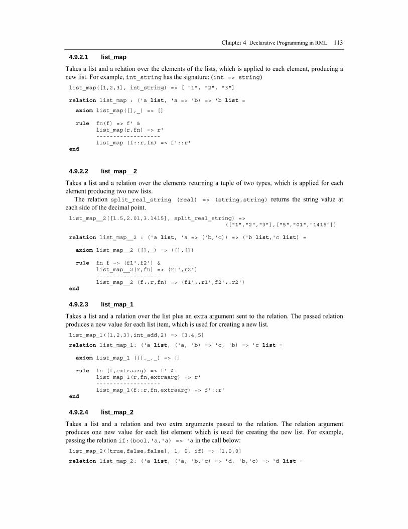
Chapter 4 Declarative Programming in RML 113
4.9.2.1 list_map
Takes a list and a relation over the elements of the lists, which is applied to each element, producing a new list. For example, int_string has the signature: (int => string) list_map([1,2,3], int_string) => [ "1", "2", "3"] relation list_map : ('a list, 'a => 'b) => 'b list =
axiom list_map([],_) => [] rule fn(f) => f' & list_map(r,fn) => r' ------------------- list_map (f::r,fn) => f'::r' end
4.9.2.2 list_map__2
Takes a list and a relation over the elements returning a tuple of two types, which is applied for each element producing two new lists.
The relation split_real_string (real) => (string,string) returns the string value at each side of the decimal point. list_map__2([1.5,2.01,3.1415], split_real_string) => (["1","2","3"],["5","01","1415"]) relation list_map__2 : ('a list, 'a => ('b,'c)) => ('b list,'c list) = axiom list_map__2 ([],_) => ([],[]) rule fn f => (f1',f2') & list_map__2(r,fn) => (r1',r2') ------------------- list_map__2 (f::r,fn) => (f1'::r1',f2'::r2') end
4.9.2.3 list_map_1
Takes a list and a relation over the list plus an extra argument sent to the relation. The passed relation produces a new value for each list item, which is used for creating a new list. list_map_1([1,2,3],int_add,2) => [3,4,5]
relation list_map_1: ('a list, ('a, 'b) => 'c, 'b) => 'c list = axiom list_map_1 ([],_,_) => [] rule fn (f,extraarg) => f' & list_map_1(r,fn,extraarg) => r' ------------------- list_map_1(f::r,fn,extraarg) => f'::r' end
4.9.2.4 list_map_2
Takes a list and a relation and two extra arguments passed to the relation. The relation argument produces one new value for each list element which is used for creating the new list. For example, passing the relation if:(bool,'a,'a) => 'a in the call below: list_map_2([true,false,false], 1, 0, if) => [1,0,0]
relation list_map_2: ('a list, ('a, 'b,'c) => 'd, 'b,'c) => 'd list =
114 Peter Fritzson Generation of Language Implementations from Structural and Natural Semantics
axiom list_map_2 ([],_,_,_) => [] rule fn (f,extraarg1,extraarg2) => f' & list_map_2(r,fn,extraarg1,extraarg2) => r' ------------------- list_map_2(f::r,fn,extraarg1,extraarg2) => f'::r' end
4.9.2.5 list_map_2_2
Takes a list and a relation with two extra arguments passed to the relation. The relation returns a tuple of two values for each list item, which are used for creating two new lists. For example, the passed relation foo(int,string,string) => (string,string) concatenates each string with itself n times, e.g.: foo(2,"a",b") => ("aa","bb") list_map_2_2 ([2,3],foo,"a","b") => [("aa","bb"),("aa","bbb")]
relation list_map_2_2: ('a list, ('a, 'b,'c) => ('d,'e), 'b,'c) => ('d * 'e) list = axiom list_map_2_2 ([],_,_,_) => [] rule fn (f,extraarg1,extraarg2) => (f1,f2) & list_map_2_2(r,fn,extraarg1,extraarg2) => r' ------------------- list_map_2_2(f::r,fn,extraarg1,extraarg2) => ((f1,f2)::r') end
4.9.2.6 list_map_0
Takes a list and a relation which does not return a value. The passed relation is probably a relation with side effects, like print. list_map_0(["a","b","c"],print) => () relation list_map_0 : ('a list, 'a => ()) => () = axiom list_map_0 ([],_) => () rule fn (f) => () & list_map_0(r,fn) => () ------------------- list_map_0(f::r,fn) => () end
4.9.2.7 list_list_map
Takes a list of lists and a relation producing one value at each call. The passed relation is applied to each element of the lists resulting in a new list of lists. list_list_map([ [1,2],[3],[4]],int_string) => [ ["1","2"],["3"],["4"] ] relation list_list_map : ('a list list, 'a => 'b) => 'b list list = axiom list_list_map ([],_) => [] rule list_map(f,fn) => f' & list_list_map(r,fn) => r' ------------------- list_list_map (f::r,fn) => f'::r' end

Chapter 4 Declarative Programming in RML 115
4.9.3 Folding, Threading, and Reversing Relations
The following are folding, threading, and list reverse operations.
4.9.3.1 list_fold
Takes a list and a relation operating on pairs of a list element and an accumulated value, together with an extra accumulating parameter which is eventually returned as the result value. The third argument is the start value for the accumulating parameter. list_fold will call the passed relation for each element in a sequence, adding to the accumulating parameter value. list_fold([1,2,3],int_add,2) => 8 int_add(1,2) => 3, int_add(2,3) => 5, int_add(3,5) => 8
relation list_fold: ('a list, ('a,'b)=> 'b, 'b) => 'b = axiom list_fold([],r,accum) => accum rule r(l,accum) => accum' list_fold(lst,r,accum') => accum2 -------------------------- list_fold(l::lst,r,accum) => accum2 end
4.9.3.2 list_list_reverse
Takes a list of lists and reverses it at both levels, i.e. both the list itself and each sublist. list_list_reverse([[1,2],[3,4,5],[6] ]) => [ [6], [5,4,3], [2,1] ] relation list_list_reverse: ('a list list) => 'a list list =
rule list_map(lsts, list_reverse) => lsts' & list_reverse(lsts') => lsts'' ----------------------- list_list_reverse(lsts) => lsts'' end
4.9.3.3 list_thread
Takes two lists of the same type and threads them together. list_thread([1,2,3],[4,5,6]) => [4,1,5,2,6,3] relation list_thread : ('a list, 'a list) => 'a list = axiom list_thread([],[]) => [] rule list_thread(ra,rb) => r' & let c = fb::r' & let d = fa::c ------------------------ list_thread(fa::ra,fb::rb) => d end
4.9.3.4 list_thread_map
Takes two lists and a relation and threads and maps the elements of the two lists creating a new list. list_thread_map([1,2],[3,4],int_add) => [1+3, 2+4] relation list_thread_map : ('a list, 'b list, ('a,'b) => 'c) => 'c list = axiom list_thread_map([],[],_) => []

116 Peter Fritzson Generation of Language Implementations from Structural and Natural Semantics
rule fn(fa,fb) => fr & list_thread_map(ra,rb,fn) => res -------------------------------- list_thread_map(fa::ra,fb::rb,fn) => fr::res end
4.9.3.5 list_thread_tuple
Takes two lists and threads the arguments into a list of tuples consisting of the two element types. list_thread_tuple([1,2,3],[true,false,true]) => [(1,true),(2,false),(3,true)] relation list_thread_tuple : ('a list, 'b list) => ('a * 'b) list = axiom list_thread_tuple([],[]) => [] rule list_thread_tuple(ra,rb) => r ----------------------------- list_thread_tuple(fa::ra, fb::rb) => ((fa,fb)::r) end
4.9.3.6 list_list_thread_tuple
Takes two list of lists as arguments and produces a list of lists of a two tuple of the element types of each list. list_list_thread_tuple([[1],[2,3]],[["a"],["b","c"]]) => [ [(1,"a")],[(2,"b"),(3,"c")] ] relation list_list_thread_tuple : ('a list list, 'b list list) => ('a * 'b) list list = axiom list_list_thread_tuple ([],[]) => [] rule list_thread_tuple(fa,fb) => f & list_list_thread_tuple(ra,rb) => r ----------------------------- list_list_thread_tuple (fa::ra, fb::rb) => f::r end
4.9.4 Union, Element Membership and Position
The following operations operates on lists in most cases as if they were sets, performing union, checking membership, etc. There are also element positioning operations.
4.9.4.1 list_position
Takes a value and a list of values and returns the (first) position the value has in the list. Position index starts at zero (??should be changed!), such that list_nth can be used on the resulting position directly. list_position(2,[0,1,2,3]) => 2 relation list_position: ('a, 'a list) => int =
rule list_pos(x, ys, 0) => n ----------------------- list_position(x, ys) => n end (** Helper relation to list_position **) relation list_pos: ('a, 'a list, int) => int =
rule x = y

Chapter 4 Declarative Programming in RML 117
----- list_pos(x, y::ys, i) => i rule not x = y & int_add(i, 1) => i' & list_pos(x, ys, i') => n ------------------------ list_pos(x, y::ys, i) => n end
4.9.4.2 list_getmember
Takes a value and a list of values and returns the value if present in the list. If not present, the relation will fail. list_getmember(0,[1,2,3]) => fail list_getmember(1,[1,2,3]) => 1 relation list_getmember: (''a, ''a list) => ''a = axiom list_getmember(_,[]) => fail rule x = y ----- list_getmember(x,y::ys) => y rule not x = y & list_getmember(x,ys) => res ---------------------- list_getmember(x,y::ys) => res end
4.9.4.3 list_deletemember
Takes a list and a value and deletes the first occurence of the value in the list. list_deletemember([1,2,3,2],2) => [1,3,2] relation list_deletemember: (''a list,''a) => ''a list =
rule list_position(elt,lst) => pos & list_delete(lst,pos) => lst' ---------------------------- list_deletemember(lst,elt) => lst' axiom list_deletemember(lst,_) => lst end
4.9.4.4 list_getmember_p
Takes a value and a list of values and a comparison relation over two values. If the value is present in the list (using the comparison relation returning true) the value is returned, otherwise the relation fails. For example, the relation equal_lenght(string,string) returns true if the strings are of same length. list_getmember_p("a",["bb","b","ccc"],equal_length) => "b" relation list_getmember_p: (''a, ''a list,(''a,''a) => bool) => ''a = axiom list_getmember_p(_,[],p) => fail rule p(x, y) => true ----- list_getmember_p(x,y::ys,p) => y
118 Peter Fritzson Generation of Language Implementations from Structural and Natural Semantics
rule p(x, y) => false & list_getmember_p(x,ys,p) => res ---------------------- list_getmember_p(x,y::ys,p) => res end
4.9.4.5 list_union_elt
Takes a value and a list of values and inserts the value into the list if it is not already in the list. If it is in the list it is not inserted. (?? Why double single quote'' in certain type names?) list_union_elt(1,[2,3]) => [1,2,3] list_union_elt(0,[0,1,2]) => [0,1,2] relation list_union_elt: (''a , ''a list) => ''a list = rule list_getmember(x,lst) => _ -------------------------- list_union_elt(x,lst) => lst rule not list_getmember(x,lst) => _ -------------------------- list_union_elt(x,lst) => x::lst end
4.9.4.6 list_union
Takes two lists and returns the union of the two lists, i.e. a list of all elements combined without duplicates. list_union([0,1],[2,1]) => [0,1,2] relation list_union: (''a list, ''a list) => ''a list = axiom list_union([],res) => res rule list_union_elt(x,lst2) => r1 & list_union(xs,r1) => res ----------------------- list_union(x::xs,lst2) => res end
4.9.4.7 list_list_union
Takes a list of lists and returns the union of the sublists. list_list_union([[1],[1,2],[3,4],[5]]) => [1,2,3,4,5] relation list_list_union: (''a list list) => ''a list = axiom list_list_union([]) => [] axiom list_list_union([x]) => x rule list_union(x1,x2) => r1 & list_list_union(r1::rest) => res ----------------------- list_list_union(x1::x2::rest) => res end
4.9.4.8 list_union_elt_p
Takes an elemement and a list and a comparison relation over the two values. It returns the list with the element inserted if not already present in the list, according to the comparison relation.

Chapter 4 Declarative Programming in RML 119
list_union_elt_p(1,[2,3],int_eq) => [1,2,3] relation list_union_elt_p: (''a , ''a list , (''a, ''a) => bool) => ''a list = rule list_getmember_p(x,lst,p) => _ -------------------------- list_union_elt_p(x,lst,p) => lst rule not list_getmember_p(x,lst,p) => _ -------------------------- list_union_elt_p(x,lst,p) => x::lst end
4.9.4.9 list_union_p
Takes two lists and a comparison relation over two elements of the list. It returns the union of the two lists, using the comparison relation passed as argument to determine identity between two elements. For example, given the relation equal_length(string,string) returning true if the strings are of same length: list_union_p(["a","aa"],["b","bbb"],equal_length) => ["a","aa","bbb"] relation list_union_p: (''a list, ''a list, (''a,''a) => bool) => ''a list = axiom list_union_p([],res,p) => res rule list_union_elt_p(x,lst2,p) => r1 & list_union_p(xs,r1,p) => res ----------------------- list_union_p(x::xs,lst2,p) => res end
4.9.4.10 list_list_union_p
Takes a list of lists and a comparison relation over two elements of the lists. It returns the union of all sublists using the comparison relation for identity. list_list_union_p([[1],[1,2],[3,4]],int_eq) => [1,2,3,4] relation list_list_union_p: (''a list list, (''a,''a) => bool) => ''a list = axiom list_list_union_p([],p) => [] axiom list_list_union_p([x],p) => x rule list_union_p(x1,x2,p) => r1 & list_list_union_p(r1::rest,p) => res ------------------------------------ list_list_union_p(x1::x2::rest,p) => res end
4.9.4.11 list_replaceat
Takes an element, a position, and a list, and replaces the value at the given position in the list. (?? zero position?) list_replaceat("A", 2, ["a","b","c"]) => ["a","b","A"] relation list_replaceat: (''a, int, ''a list) => ''a list = (*axiom list_replaceat(x,-1,[]) => []*) axiom list_replaceat (x,0,y::ys) => x::ys

120 Peter Fritzson Generation of Language Implementations from Structural and Natural Semantics
rule int_ge(n,1) => true & int_sub(n,1) => nn & list_replaceat(x,nn,ys) => res ----------------------------- list_replaceat(x,n,y::ys) => y::res (* rule print "-list_replaceat failed\n" ----------------------- list_replaceat(_,_,_) => fail*) (*??*) end
4.9.4.12 list_replaceat_withfill
Takes an element, a position, a list, and a fill value. The relation replaces the value at the given position in the list, if the given position is out of range, the fill value is used to padd the list up to that element position and then insert the value at the position. list_replaceat_withfill("A", 5, ["a","b","c"],"dummy") => ["a","b","c","dummy","A"] relation list_replaceat_with_fill: (''a, int, ''a list,''a) => ''a list = axiom list_replaceat_with_fill (x,0,y::ys,fillv) => x::ys axiom list_replaceat_with_fill(x,1,[],fillv) => [fillv,x] rule int_gt(numfills,1) => true & int_sub(numfills,1) => numfills' & list_fill(fillv,numfills') => res & list_append(res,[x]) => res' --------------------------------- list_replaceat_with_fill(x,numfills,[],fillv) => res' rule int_ge(n,1) => true & int_sub(n,1) => nn & list_replaceat_with_fill(x,nn,ys,fillv) => res ---------------------------------------------- list_replaceat_with_fill(x,n,y::ys,fillv) => y::res end
4.9.4.13 split_tuple2_list
Takes a list of two-tuples and splits it into two lists. split_tuple2_list([("a",1),("b",2),("c",3)]) => (["a","b","c"], [1,2,3]) relation split_tuple2_list : ('a * 'b) list => ('a list, 'b list) =
axiom split_tuple2_list([]) => ([],[]) rule split_tuple2_list(rest) => (xs,ys) --------------------------------- split_tuple2_list((x,y)::rest) => (x::xs, y::ys) end
4.9.5 Reduction Operations
These relations reduces a list to a single value, sometimes using a reduction operation passed as an argument.
4.9.5.1 list_reduce
Takes a list and a relation operating on two elements of the list at a time. The relation performs a reduction of the list to a single value using the passed relation.
Chapter 4 Declarative Programming in RML 121
list_reduce([1,2,3],int_add) => 6 relation list_reduce: ('a list, ('a,'a) => 'a) => 'a =
axiom list_reduce([e],r) => e rule r(a,b) => res ------------- list_reduce([a,b],r) => res rule r(a,b) => res1 & list_reduce(xs,r) => res2 & r(res1,res2) => res ------------------- list_reduce(a::b::(xs as _::_),r) => res end
4.9.5.2 string_append_list
Takes a list of strings and appends them. string_append_list(["foo", " ", "bar"]) => "foo bar" relation string_append_list : (string list) => string = axiom string_append_list([]) => "" axiom string_append_list([f]) => f rule string_append_list r => r' & string_append(f,r') => str --------------------------- string_append_list f::r => str end
4.9.5.3 string_delimit_list
Takes a list of strings and a string delimiter and appends all list elements with the string delimiter inserted between elements. string_delimit_list(["x","y","z"], ", ") => "x, y, z" relation string_delimit_list : (string list, string) => string = axiom string_delimit_list([],_) => "" axiom string_delimit_list([f],delim) => f rule string_delimit_list(r,delim) => str1 & string_append(f,delim) => str2 & string_append(str2,str1) => str --------------------------- string_delimit_list(f::r,delim) => str end
4.9.5.4 bool_or_list
Takes a list of boolean values and applies the boolean or operator to the list elements. bool_or_list([true,false,false]) => true bool_or_list([false,false,false]) => false relation bool_or_list: bool list => bool = axiom bool_or_list([b]) => b

122 Peter Fritzson Generation of Language Implementations from Structural and Natural Semantics
rule b = true --------------------- bool_or_list(b::rest) => true rule b = false & bool_or_list(rest) => res --------------------- bool_or_list(b::rest) => res end
4.9.5.5 bool_and_list
Takes a list of boolean values and applies the boolean 'and' operator on the elements. bool_and_list([true, true]) => true bool_and_list([false,false,true]) => false relation bool_and_list: bool list => bool = axiom bool_and_list([b]) => b rule b = false --------------------- bool_and_list(b::rest) => false rule b = true & bool_and_list(rest) => res --------------------- bool_and_list(b::rest) => res end
4.9.6 Miscellaneous
The following are miscellaneous utility operations.
4.9.6.1 if
Takes a boolean and two values. Returns the first value (second argument) if the boolean value is true, otherwise the second value (third argument) is returned. if(true,"a","b") => "a" relation if : (bool,'a,'a) => 'a =
axiom if (true,r,_) => r axiom if (false,_,r) => r end
4.9.6.2 bool_string
Takes a boolean value and returns a string representation of the boolean value. bool_string(true) => "true" relation bool_string: bool => string = axiom bool_string true => "true" axiom bool_string false => "false" end
4.9.6.3 string_equal
Takes two strings and returns true if the strings are equal. (?? Is this not already builtin?)

Chapter 4 Declarative Programming in RML 123
string_equal("a","a") => true relation string_equal: (string,string) => bool =
rule a = b ----- string_equal(a,b) => true axiom string_equal(_,_) => false end
4.9.6.4 list_matching
Takes a list of values and a matching relation over the values and returns a sublist of values for which the matching relation succeeds. For example, given the relation is_numeric(string) => () which succeeds if the string is numeric. list_matching(["foo","1","bar","4"],is_numeric) => ["1","4"] relation list_matching: ('a list, 'a => () ) => 'a list = axiom list_matching ([],_) => [] rule cond(v) & list_matching (vl, cond) => vl' ------------------- list_matching (v::vl, cond) => v::vl' rule not cond(v) & list_matching (vl, cond) => vl' -------------------------- list_matching (v::vl, cond) => vl' end
4.9.6.5 apply_option
Takes an option value and a relation that can transform the value. It returns the transformed value in another option value, resulting from the application of the passed relation to the value. apply_option(SOME(1), int_string) => SOME("1") apply_option(NONE, int_string) => NONE relation apply_option : ('a option,'a => 'b) => 'b option = axiom apply_option(NONE,_) => NONE rule rel(a) => b ----------- apply_option( SOME(a),rel) => SOME(b) end
4.9.6.6 list_split
Takes a list of values and a position value. (?? update zero postions?) The relation returns the list split into two lists at the position given as argument. list_split([1,2,5,7],2) => ([1,2],[5,7]) relation list_split : ('a list, int) => ('a list, 'a list) =
axiom list_split(a,0) => ([],a) rule list_length(a) => length & int_gt(index,length) => true &

124 Peter Fritzson Generation of Language Implementations from Structural and Natural Semantics
print "Index out of bounds (greater than list length) in relation list_split\n" ---------------- list_split(a,index) => fail rule int_lt(index,0) => true & print "Index out of bounds (less than zero) in relation list_split\n" ---------------- list_split(a,index) => fail rule int_ge(index,0) => true & list_length(a) => length & int_le(index,length) => true & list_split2(a,[],index) => (b,c) ---------------- list_split(a,index) => (c,b) end (** helper relation to list_split **) relation list_split2 : ('a list, 'a list, int) => ('a list, 'a list) = rule int_eq(index,0) => true ------------------ list_split2(a,b,index) => (a,b) rule int_sub(index,1) => new_index & list_append(b,[a]) => c & list_split2(rest,c,new_index) =>(c,d) ------------------ list_split2(a::rest,b,index) => (c,d)
rule print "list_split2 failed\n" ---------------- list_split2(_,_,_) => fail end
4.10 Lookup Mechanisms Lookup functions/relations are needed for accessing and storing identifier bindings in environments during semantic processing. From the pure semantics point of view, the actual choice of environment data structure and formulation of lookup mechanism does not matter – just the lookup behavior itself is importan. However, from a practical point of view the performance of the lookup function is quite important when generating interpreters or compilers from the specification. A slow implementation of the lookup mechanism will give a slow interpreter or compiler.
4.10.1 Lookup through Linear Search
The relation lookup looks up identifier bindings in the environment, see Section 2.5.4.1 for a detailed explanation and Section 6.8 for its use in the specification for the Petrol language.
x 35 y 135 z 1350
Environment
z1000 999
Figure 4-1. An environment represented as a linked list, containing name-value pairs for x, y, z, ... z1000.
The definition of the linked-list lookup relation is shown once more below:

Chapter 4 Declarative Programming in RML 125
relation lookup: (Env, Ident) => Bnd =
rule key1 = key0 ---------------- lookup((key1,value)::_, key0) => bnd rule not key1 = key0 & lookup(env, key0) => bnd ---------------- lookup((key1,_)::env, key0) => bnd end
This lookup implementation performs a linear search through a linked list representation of the environment, which gives low performance if the environment contains many bindings. If the number of bindings is N, the execution time has complexity O(N2), i.e., quadratic complexity.
4.10.2 Lookup through Binary Search
????Insert text
4.10.2.1 The Binary Tree Data Structure
The binary tree data structure used for the environment is generic and can be used in any RML application.
TREENODE
TREENODEINTconst
12
INTconst
5 13
TFREEVALUE
TREEVALUEINTconst
Figure 4-2. Binary tree for lookup according to the BinTree and TreeValue declarations. (??update figure).
The BinSearch module starts with the module name followed by declarations of data structures and relation signatures. module BinSearch:
The tree data structure BinTree is defined as follows: datatype BinTree = TREENODE of TreeValue option * (* Value *) BinTree option * (* Left subtree *) BinTree option (* Right subtree *)
Each node in the binary tree can have a tree value associated with it: datatype TreeValue = TREEVALUE of Key * Value type Ident = string type Key = Ident type Value = int (* or some other kind of value *) relation tree_lookup: (BinTree, Key, Key => int) => Value relation tree_add: (BinTree, Key, Value, Key => int) => (BinTree) relation myhash: Key => int

126 Peter Fritzson Generation of Language Implementations from Structural and Natural Semantics
end
The implementation of the binary lookup mechanism. (* Hash function, from key string to integer *) relation myhash: Key => int = rule System.hash(str) => res ------------ myhash(str) => res end (* Creation of new empty tree *) relation tree_new: () => BinTree = axiom tree_new() => TREENODE(NONE,NONE,NONE) end
4.10.2.2 Lookup in an Existing Tree
lkjlkj
lklkjsdfsdf relation tree_lookup: (BinTree, Key, Key => int) => Value = rule rkey = key --------------- tree_lookup (TREENODE(SOME(TREEVALUE(rkey,rval)),left,right), key,hashfunc) => rval rule (* Search to the right*) hashfunc(key) => hval & hashfunc(rkey) => rhval & int_gt(hval,rhval) => true & tree_lookup(right,key,hashfunc) => res -------------------- tree_lookup(TREENODE(SOME(TREEVALUE(rkey,rval)),left,SOME(right)), key,hashfunc) => res rule (* Search to the left*) hashfunc(key) => hval & hashfunc(rkey) => rhval & int_le(hval,rhval) => true & tree_lookup(left,key,hashfunc) => res -------------------- tree_lookup(TREENODE(SOME(TREEVALUE(rkey,rval)),SOME(left),right), key,hashfunc) => res end
4.10.2.3 Insertion of New Nodes
lkjlkjljk lkjlkj ???

Chapter 4 Declarative Programming in RML 127
TREENODE
TREENODEINTconst
12
INTconst
5
INTconst
13
TREEVALUE
TREEVALUE
Figure 4-3. Binary tree for lookup (??update figure).
lkjkjl??? relation tree_add: (BinTree, Key, Value, Key => int) => (BinTree) = axiom tree_add (TREENODE(NONE,NONE,NONE),key,value,_) => TREENODE(SOME(TREEVALUE(key,value)),NONE,NONE) rule (* Replace this node *) rkey = key --------------- tree_add(TREENODE(SOME(TREEVALUE(rkey,rval)),left,right), key,value, hashfunc) => (TREENODE(SOME(TREEVALUE(rkey,value)),left,right)) rule (* Insert to right subtree*) hashfunc(key) => hval & hashfunc(rkey) => rhval & int_gt(hval,rhval) => true & tree_add(t,key,value,hashfunc) => t' ------------------------ tree_add (TREENODE(SOME(TREEVALUE(rkey,rval)),left, right as SOME(t)),key,value,hashfunc) => (TREENODE(SOME(TREEVALUE(rkey,rval)),left,SOME(t'))) rule (* Insert to right node*) hashfunc(key) => hval & hashfunc(rkey) => rhval & int_gt(hval,rhval) => true & tree_add(TREENODE(NONE,NONE,NONE),key,value,hashfunc) => right' ------------------------ tree_add (TREENODE(SOME(TREEVALUE(rkey,rval)),left, right as NONE),key,value,hashfunc) => (TREENODE(SOME(TREEVALUE(rkey,rval)),left,SOME(right'))) rule (* Insert to left subtree*) hashfunc(key) => hval & hashfunc(rkey) => rhval & int_le(hval,rhval) => true & tree_add(t,key,value,hashfunc) => t' ------------------------ tree_add (TREENODE(SOME(TREEVALUE(rkey,rval)), left as SOME(t),right),key,value,hashfunc) => (TREENODE(SOME(TREEVALUE(rkey,rval)),SOME(t'),right)) rule (* Insert to left node*) hashfunc(key) => hval & hashfunc(rkey) => rhval & int_le(hval,rhval) => true & tree_add(TREENODE(NONE,NONE,NONE),key,value,hashfunc) => left' ------------------------ tree_add (TREENODE(SOME(TREEVALUE(rkey,rval)), left as NONE,right),key,value,hashfunc) => (TREENODE(SOME(TREEVALUE(rkey,rval)),SOME(left'),right)) rule print "tree_add failed\n"

128 Peter Fritzson Generation of Language Implementations from Structural and Natural Semantics
----------------------- tree_add(_,_,_,_) => fail end
(BRK)
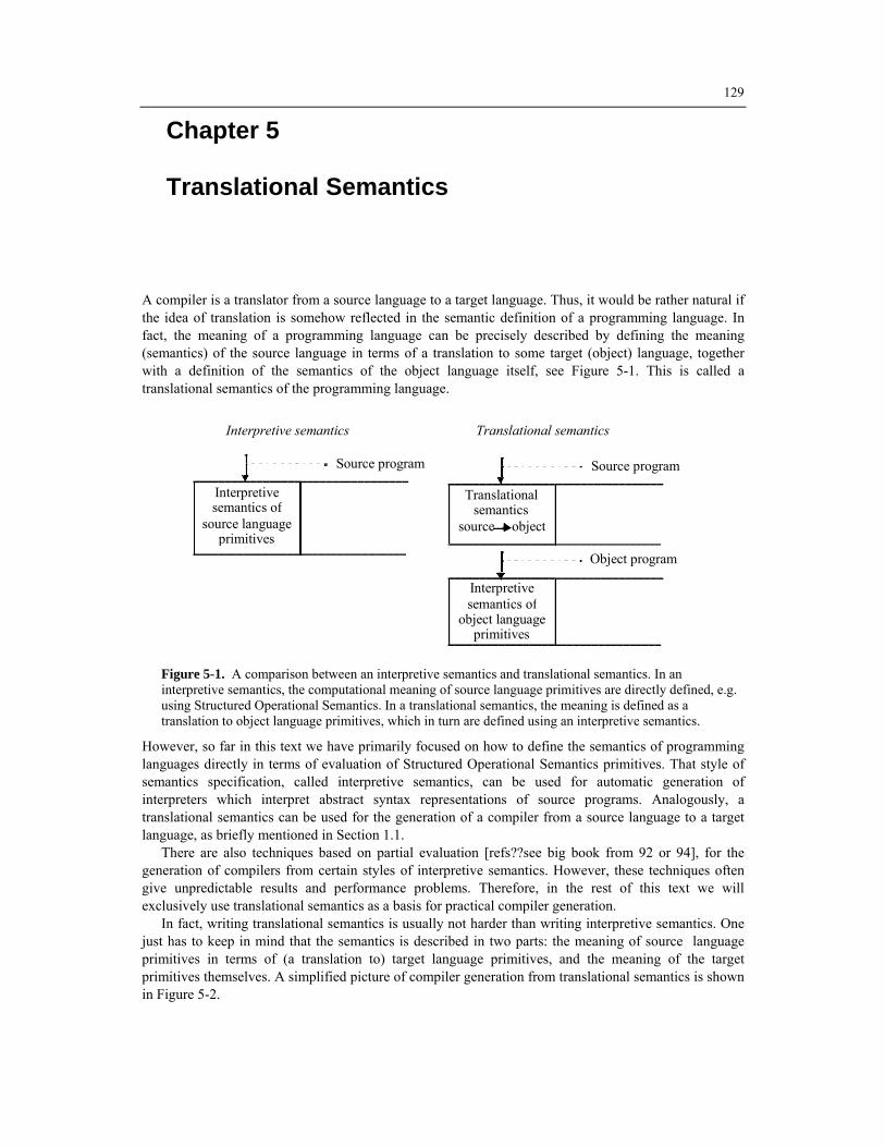
129
Chapter 5 Translational Semantics
A compiler is a translator from a source language to a target language. Thus, it would be rather natural if the idea of translation is somehow reflected in the semantic definition of a programming language. In fact, the meaning of a programming language can be precisely described by defining the meaning (semantics) of the source language in terms of a translation to some target (object) language, together with a definition of the semantics of the object language itself, see Figure 5-1. This is called a translational semantics of the programming language.
Interpretive semantics Translational semantics
Translational
Interpretive
Source program
Object program
Interpretive
Source program
semantics of semantics
semantics of
source object
object languageprimitives
source language primitives
Figure 5-1. A comparison between an interpretive semantics and translational semantics. In an interpretive semantics, the computational meaning of source language primitives are directly defined, e.g. using Structured Operational Semantics. In a translational semantics, the meaning is defined as a translation to object language primitives, which in turn are defined using an interpretive semantics.
However, so far in this text we have primarily focused on how to define the semantics of programming languages directly in terms of evaluation of Structured Operational Semantics primitives. That style of semantics specification, called interpretive semantics, can be used for automatic generation of interpreters which interpret abstract syntax representations of source programs. Analogously, a translational semantics can be used for the generation of a compiler from a source language to a target language, as briefly mentioned in Section 1.1.
There are also techniques based on partial evaluation [refs??see big book from 92 or 94], for the generation of compilers from certain styles of interpretive semantics. However, these techniques often give unpredictable results and performance problems. Therefore, in the rest of this text we will exclusively use translational semantics as a basis for practical compiler generation.
In fact, writing translational semantics is usually not harder than writing interpretive semantics. One just has to keep in mind that the semantics is described in two parts: the meaning of source language primitives in terms of (a translation to) target language primitives, and the meaning of the target primitives themselves. A simplified picture of compiler generation from translational semantics is shown in Figure 5-2.

130 Peter Fritzson Generation of Language Implementations from Structural and Natural Semantics
Trans. SemanticsTranslation toobject code
Formalism Compiler phase Program representation Generator tool
Regular expressions
BNF grammar
Natural semantics in RML
Lex Scanner
Yacc Parser
Text
Token sequence
Abstract syntax
Machine code
rml2c
Figure 5-2. Simplified version of compiler generation based on translational semantics. The semantics of a language is specified directly in terms of object code primitives. In comparison to Figure 1-1, the optimization and final code generation phases have been excluded.
5.1 Translating PAM to Machine Code As an introduction translational semantics, we will specify the translational semantics of a simple language, with the goal of generating a compiler from this language to machine code. The simple PAM language has already been described, and an interpretive semantics has been given in Section 2.6. This makes it a natural first choice for a translational semantics. In Chapter 3 of [ref Pagan], an attribute grammar style translational semantics of PAM can be found. It is instructive to compare the attribute grammar specification to the Structured Operational Semantics style translational semantics of PAM described in this chapter. The target assembly language described in the next section has been chosen to be the same as in [ref Pagan] to simplify parallel study.
5.1.1 A Target Assembly Language
In the translational approach, a target language for the translation process is needed. Here we choose a very simple assembly (machine code) language, which is similar to realistic assembly languages, but very much simplified. For example, this machine has only one register (an accumulator) and much fewer instructions than commercial microprocessors. Still, it is complete enough to reflect most properties of realistic assembly languages. There are 17 types of instructions, listed below: LOAD Load accumulator STO Store ADD Add SUB Subtract MULT Multiply DIV Divide GET Input a value PUT Output a value J Jump JN Jump on negative JP Jump on positive JNZ Jump on negative or zero JPZ Jump on positive or zero JNP Jump on negative or positive LAB Label (no operation) HALT Halt execution

Chapter 5 Translational Semantics 131
All instructions, except HALT, have one operand. For example, LOAD X, will load the variable at address X into the accumulator. Conversely, STO X will store the current value in the accumulator at the address specified by X. The instructions ADD, SUB, MULT, and DIV perform arithmetic operations on two values, the accumulator value and the operand value. Operands can be integer constants or symbolic addresses of variables or temporaries (T1,T2,...), or symbolic labels representing code addresses. Instructions which compute a result always store it in the accumulator. For example, SUB X means that accumulator-X is computed, and stored in the accumulator.
The input/output instructions GET X and PUT X will input and output a value to variable X, respectively. There are 5 conditional jump instructions and one unconditional jump. The conditional jumps are: JN,JP,JNZ,JPZ, and JNP which jump to a label (address) conditionally on the current value in the accumulator. The J L1 instruction is an example of an unconditional jump to the label L1. The LAB pseudo instruction is no instruction, it just declares the position of a label in the code. Finally, the HALT instruction stops execution.
5.1.2 A Translated PAM Example Program
Before going into the details of the translational semantics, it is instructive to take a look at the translation of a small PAM example PAM program, shown below: read x,y; while x<> 99 do ans := (x+1) - (y / 2); write ans; read x,y; end
This example program is translated into the following assembly code, presented in its textual representation: GET x STO T1 GET y LOAD T0 L2 LAB SUB T1 LOAD x STO ans SUB 99 PUT ans JZ L3 GET x LOAD x GET y ADD 1 J L2 STO T0 L3 LAB LOAD y HALT DIV 2
However, to simplify and structure the translational semantics of PAM, the target language will be a structured representation of the assembly code, called MCode, which is defined in RML. The MCode representation of the translated program, as shown below, is finally converted into the textual representation previously presented.
All MCode operators start with the letter M. Binary arithmetic operators are grouped under the node MB, and conditional jump operators under MJ. There are four kinds of operands, indicated by the constructors I (Identifier), L (Label), N (Numeric integer), and T (for Temporary). MGET( I(x) ) MSTO( T(2) ) MGET( I(y) ) MLOAD( T(1) ) MLABEL( L(1) ) MB(MSUB,T(2) ) MLOAD( I(x) ) MSTO( I(ans) ) MB(MSUB,N(99) ) MPUT( I(ans) ) MJ(MJZ, L(2) ) MGET( I(x) ) MLOAD( I(x) ) MGET( I(y) ) MB(MADD,N(1) ) MJMP( L(1) ) MSTO( T(1) ) MLABEL( L(2) ) MLOAD( I(y) ) MHALT

132 Peter Fritzson Generation of Language Implementations from Structural and Natural Semantics
MB(MDIV,N(2) )
5.1.3 Abstract Syntax for Machine Code Intermediate Form
The abstract syntax of the structured machine code representation, called MCode, is defined in RML below. We group the four arithmetic binary operators MADD, MSUB, MMULT and MDIV in the union type MBinOp. The six conditional jump instructions MJMP,MJP,MJN,MJNZ,MJPZ,MJZ are represented by constructors in the union type MCondJmp. As usual, this grouping of similar constructs simplifies the semantic description. There are four kinds of operands: identifiers, numeric constants, labels, and temporaries. For these we have defined the type aliases MLab, MTemp, MIdent, MidTemp in order to make the translational semantics more readable.
The constructors MB and MJ are used for binary arithmetic instructions and conditional jumps, respectively. The first argument to these constructors indicates the specific arithmetic operation or conditional jump. type Id = string datatype MBinOp = MADD | MSUB | MMULT | MDIV datatype MCondJmp = MJNP | MJP | MJN | MJNZ | MJPZ | MJZ datatype MOperand = I of Id | N of int | T of int type MLab = L of int type MTemp = T of int type MIdent = I of Id type MIdTemp = I of Id | T of int datatype MCode = MB of MBinOp * Moperand (* Binary arith ops *) | MJ of MCondJmp * MLab (* Conditional jumps *) | MJMP of Mlab | MLOAD of MIdTemp | MSTO of MIdTemp | MGET of MIdent | MPUT of MIdent | MLABEL of MLab | MHALT
5.1.4 Concrete Syntax of PAM
The concrete syntax of PAM has already been described in Section 2.6.2.
5.1.5 Abstract Syntax of PAM
The abstract syntax of PAM is identical to that described in Section 2.6.3. It is repeated here for convenience. module Absyn: (* Parameterized abstract syntax for the PAM language *) type Ident = string datatype BinOp = ADD | SUB | MUL | DIV datatype RelOp = EQ | GT | LT | LE | GE | NE datatype Exp = INT of int | IDENT of Ident | BINARY of Exp * BinOp * Exp | RELATION of Exp * RelOp * Exp type Comparison = Exp datatype Stmt = ASSIGN of Ident * Exp (* Id := Exp *) | IF of Exp * Stmt * Stmt (* if Exp then Stmt..*) | WHILE of Exp * Stmt (* while Exp do Stmt*)

Chapter 5 Translational Semantics 133
| TODO of Exp * Stmt (* to Exp do Stmt...*) | READ of Ident list (* read id1,id2,...*) | WRITE of Ident list (* write id1,id2,..*) | SEQ of Stmt * Stmt (* Stmt1; Stmt2 *) | SKIP (* ; empty stmt *) end (* of interface section of module Absyn *)
5.1.6 Translational Semantics of PAM
The translational semantics of PAM consists of several separate parts. First we describe the translation of arithmetic expressions, which is the simplest case. Then we turn to comparison expressions which occur in the conditional part of if-statements and while-statements. Such comparisons are translated into conditional jump instructions. Next, the translation of all statement types in PAM are described together with the translation of a whole program. Finally, an RML program for emitting assembly text from the structured MCode representation is presented, although this is not really part of the translational semantics of PAM.
5.1.6.1 Arithmetic Expression Translation
The translation of binary arithmetic expressions is specified by the trans_expr relation together with two small help relations trans_binop and gentemp. The trans_binop function just translates the four arithmetic node types in the abstract syntax into corresponding MCode node types. Each call to the gentemp generator function produces a unique label of type L1, L2, etc.
The trans_expr relation contains essentially all semantics of PAM arithmetic expressions. The first two axioms handle the simple cases of expressions which are either an integer constant or a variable. The generated code is in the form of a list of MCode tuples, as is reflected in the signature of the trans_expr relation below: relation trans_expr: Exp => Mcode list = axiom trans_expr(INT(v)) => [MLOAD( N(v))] (* integer v *) axiom trans_expr(IDENT(id)) => [MLOAD( I(id))] (* identifier id *) ....
The semantics of computing a constant or a variable is to load the value into the accumulator, as in the following instruction where id is the variable X4: MLOAD( I(X4) )
and in assembly text form: LOAD X4
The first rule is for simple binary arithmetic expressions such as e1 - e2 where expression e2 only is a constant or a variable which gives rise to a load instruction (see the second premise in the rule). The code for this expression is as follows, where MB denotes a binary operator and MSUB subtraction: <code for expression e1> MB(MSUB ( e2))
and in assembly text form: <code for expression e1> SUB e2
The corresponding RML rule follows below. rule trans_expr(e1) => cod1 & trans_expr(e2) => [MLOAD(operand2)] & (* expr2 simple *) trans_binop(binop) => opcode & list_append(cod1, [MB(opcode,operand2)]) => cod3

134 Peter Fritzson Generation of Language Implementations from Structural and Natural Semantics
----------------------------------- (* expr1 binop expr2 *) trans_expr(BINARY(e1,binop,e2)) => cod3
The second rule handles binary arithmetic expressions such as e1-e2, e1+e2, etc., where e2 can be a complicated expression. The code pattern for e1-e2 in assembly text form becomes: <code for e1> STO T1
<code for e2> STO T2 LOAD T1 SUB T2
The rule is presented below. The generated code for expressions e1 and e2 are bound to cod1 and cod2, respectively. The binary operation is translated to the MCode version, which is bound to opcode. Then two temporaries are produced. Finally a code sequence is produced which closely follows the code pattern above. The function list_append6 appends the elements of six argument lists, whereas the standard list_append only accepts two list arguments. rule trans_expr(e1) => cod1 & trans_expr(e2) => cod2 & trans_binop(binop) => opcode & gentemp => t1 & gentemp => t2 & list_append6( cod1, (* code for expr1 *) [MSTO(t1)], (* store expr1 *) cod2, (* code for expr2 *)= [MSTO(t2)], (* store expr2 *) [MLOAD(t1)], (* load expr1 value into Acc *) [MB(opcode,t2)] ) => cod3 (* Do arith operation *) ----------------------------------- (* expr1 binop expr2 *) trans_expr(BINARY(e1,binop,e2)) => cod3
As one additional example, we show the following expression: (x + y*z) + b*c
which is translated into the code sequence: LOAD x STO T3 STO T1 LOAD b LOAD y MULT c MULT z STO T4 STO T2 LOAD T3 LOAD T1 ADD T4 ADD T2
Note that the two rules for binary arithmetic operations overlap. The first rule covers the simple case where the second expression is just an identifier or constant, and will give rise to more compact code than the second rule which covers both the simple and the general case. From a semantic point of view, the first rule is not needed since the second rule specifies the same semantics for simple arithmetic expressions as the second rule, even though the second rule will give rise to more instructions in the translated code. Still, it is not incorrect to keep the first rule, since the PAM semantics is not changed by it.
Operationally, RML will evaluate the rules in top-down order, and thus will use the more specific first rule whenever it matches. Therefore we keep the first rule in order to obtain a compiler that produces slightly more efficient code than otherwise possible.
The complete trans_expr relation follows below, together with some help relations:
(*************** Arithmetic expression translation **************)
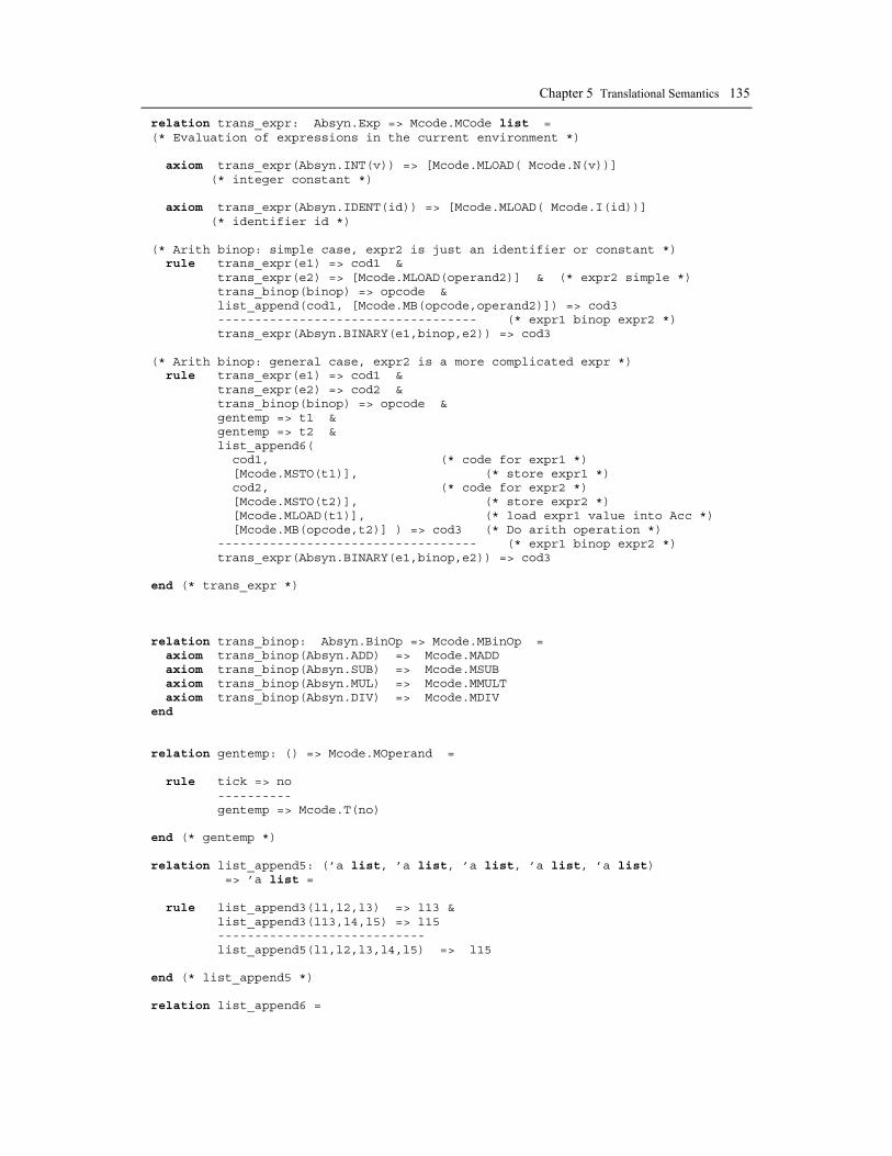
Chapter 5 Translational Semantics 135
relation trans_expr: Absyn.Exp => Mcode.MCode list = (* Evaluation of expressions in the current environment *) axiom trans_expr(Absyn.INT(v)) => [Mcode.MLOAD( Mcode.N(v))] (* integer constant *) axiom trans_expr(Absyn.IDENT(id)) => [Mcode.MLOAD( Mcode.I(id))] (* identifier id *) (* Arith binop: simple case, expr2 is just an identifier or constant *) rule trans_expr(e1) => cod1 & trans_expr(e2) => [Mcode.MLOAD(operand2)] & (* expr2 simple *) trans_binop(binop) => opcode & list_append(cod1, [Mcode.MB(opcode,operand2)]) => cod3 ----------------------------------- (* expr1 binop expr2 *) trans_expr(Absyn.BINARY(e1,binop,e2)) => cod3 (* Arith binop: general case, expr2 is a more complicated expr *) rule trans_expr(e1) => cod1 & trans_expr(e2) => cod2 & trans_binop(binop) => opcode & gentemp => t1 & gentemp => t2 & list_append6( cod1, (* code for expr1 *) [Mcode.MSTO(t1)], (* store expr1 *) cod2, (* code for expr2 *) [Mcode.MSTO(t2)], (* store expr2 *) [Mcode.MLOAD(t1)], (* load expr1 value into Acc *) [Mcode.MB(opcode,t2)] ) => cod3 (* Do arith operation *) ----------------------------------- (* expr1 binop expr2 *) trans_expr(Absyn.BINARY(e1,binop,e2)) => cod3 end (* trans_expr *) relation trans_binop: Absyn.BinOp => Mcode.MBinOp = axiom trans_binop(Absyn.ADD) => Mcode.MADD axiom trans_binop(Absyn.SUB) => Mcode.MSUB axiom trans_binop(Absyn.MUL) => Mcode.MMULT axiom trans_binop(Absyn.DIV) => Mcode.MDIV end relation gentemp: () => Mcode.MOperand = rule tick => no ---------- gentemp => Mcode.T(no) end (* gentemp *) relation list_append5: (’a list, ’a list, ’a list, ’a list, ’a list) => ’a list = rule list_append3(l1,l2,l3) => l13 & list_append3(l13,l4,l5) => l15 ---------------------------- list_append5(l1,l2,l3,l4,l5) => l15 end (* list_append5 *) relation list_append6 =
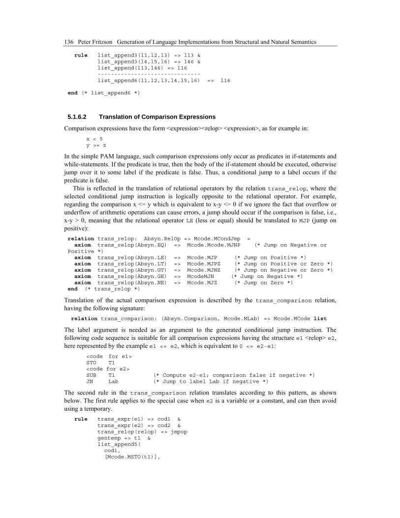
136 Peter Fritzson Generation of Language Implementations from Structural and Natural Semantics
rule list_append3(l1,l2,l3) => l13 & list_append3(l4,l5,l6) => l46 & list_append(l13,l46) => l16 ------------------------------- list_append6(l1,l2,l3,l4,l5,l6) => l16 end (* list_append6 *)
5.1.6.2 Translation of Comparison Expressions
Comparison expressions have the form <expression><relop> <expression>, as for example in: x < 5 y >= z
In the simple PAM language, such comparison expressions only occur as predicates in if-statements and while-statements. If the predicate is true, then the body of the if-statement should be executed, otherwise jump over it to some label if the predicate is false. Thus, a conditional jump to a label occurs if the predicate is false.
This is reflected in the translation of relational operators by the relation trans_relop, where the selected conditional jump instruction is logically opposite to the relational operator. For example, regarding the comparison x <= y which is equivalent to x-y <= 0 if we ignore the fact that overflow or underflow of arithmetic operations can cause errors, a jump should occur if the comparison is false, i.e., x-y > 0, meaning that the relational operator LE (less or equal) should be translated to MJP (jump on positive): relation trans_relop: Absyn.RelOp => Mcode.MCondJmp = axiom trans_relop(Absyn.EQ) => Mcode.Mcode.MJNP (* Jump on Negative or Positive *) axiom trans_relop(Absyn.LE) => Mcode.MJP (* Jump on Positive *) axiom trans_relop(Absyn.LT) => Mcode.MJPZ (* Jump on Positive or Zero *) axiom trans_relop(Absyn.GT) => Mcode.MJNZ (* Jump on Negative or Zero *) axiom trans_relop(Absyn.GE) => McodeMJN (* Jump on Negative *) axiom trans_relop(Absyn.NE) => Mcode.MJZ (* Jump on Zero *) end (* trans_relop *)
Translation of the actual comparison expression is described by the trans_comparison relation, having the following signature: relation trans_comparison: (Absyn.Comparison, Mcode.MLab) => Mcode.MCode list
The label argument is needed as an argument to the generated conditional jump instruction. The following code sequence is suitable for all comparison expressions having the structure e1 <relop> e2, here represented by the example e1 <= e2, which is equivalent to 0 <= e2-e1: <code for e1> STO T1 <code for e2> SUB T1 (* Compute e2-e1; comparison false if negative *) JN Lab (* Jump to label Lab if negative *)
The second rule in the trans_comparison relation translates according to this pattern, as shown below. The first rule applies to the special case when e2 is a variable or a constant, and can then avoid using a temporary. rule trans_expr(e1) => cod1 & trans_expr(e2) => cod2 & trans_relop(relop) => jmpop gentemp => t1 & list_append5( cod1, [Mcode.MSTO(t1)],

Chapter 5 Translational Semantics 137
cod2, [Mcode.MB(Mcode.MSUB,t1)], [Mcode.MJ(jmpop,lab)] ) => cod3 ----------------------------------- (* expr1 relop expr2 *) trans_comparison(Absyn.RELATION(e1,relop,e2),lab) => cod3
The special relations needed for translation of comparison expressions follow below:
(*************** Comparison expression translation **************) relation trans_comparison: (Absyn.Comparison, Mcode.MLab) => Mcode.MCode list = (* translation of a comparison: expr1 relation expr2 * Example call: trans_comparison(RELATION(INDENT(x), GT, INT(5)), L(10)) * * Use a simple code pattern (the first rule), when expr2 is a simple * identifier or constant: * code for expr1 * SUB operand2 * conditional jump to lab * * or a general code pattern (second rule), which is needed when expr2 * is more complicated than a simple identifier or constant: * code for expr1 * STO temp1 * code for expr2 * SUB temp1 * conditional jump to lab *) rule trans_expr(e1) => cod1 & trans_expr(e2) => [Mcode.MLOAD(operand2)] & trans_relop(relop) => jmpop & list_append3( cod1, [Mcode.MB(Mcode.MSUB, operand2)], [Mcode.MJ(jmpop,lab)] ) => cod3 ----------------------------------- (* expr1 relop expr2 *) trans_comparison(Absyn.RELATION(e1,relop,e2),lab) => cod3 rule trans_expr(e1) => cod1 & trans_expr(e2) => cod2 & trans_relop(relop) => jmpop gentemp => t1 & list_append5( cod1, [Mcode.MSTO(t1)], cod2, [Mcode.MB(Mcode.MSUB,t1)], [Mcode.MJ(jmpop,lab)] ) => cod3 ----------------------------------- (* expr1 relop expr2 *) trans_comparison(Absyn.RELATION(e1,relop,e2),lab) => cod3 end (* trans_comparison *) relation trans_relop: Absyn.RelOp => Mcode.MCondJmp = (* Note that for these relational operators, the selected jump * instruction is logically opposite. For example, if equality to zero * is true, we should should just continue, otherwise jump (MJNP) *) axiom trans_relop(Absyn.EQ) => Mcode.MJNP (* Jump on Negative or Positive*) axiom trans_relop(Absyn.LE) => Mcode.MJP (* Jump on Positive *) axiom trans_relop(Absyn.LT) => Mcode.MJPZ (* Jump on Positive or Zero *) axiom trans_relop(Absyn.GT) => Mcode.MJNZ (* Jump on Negative or Zero *)
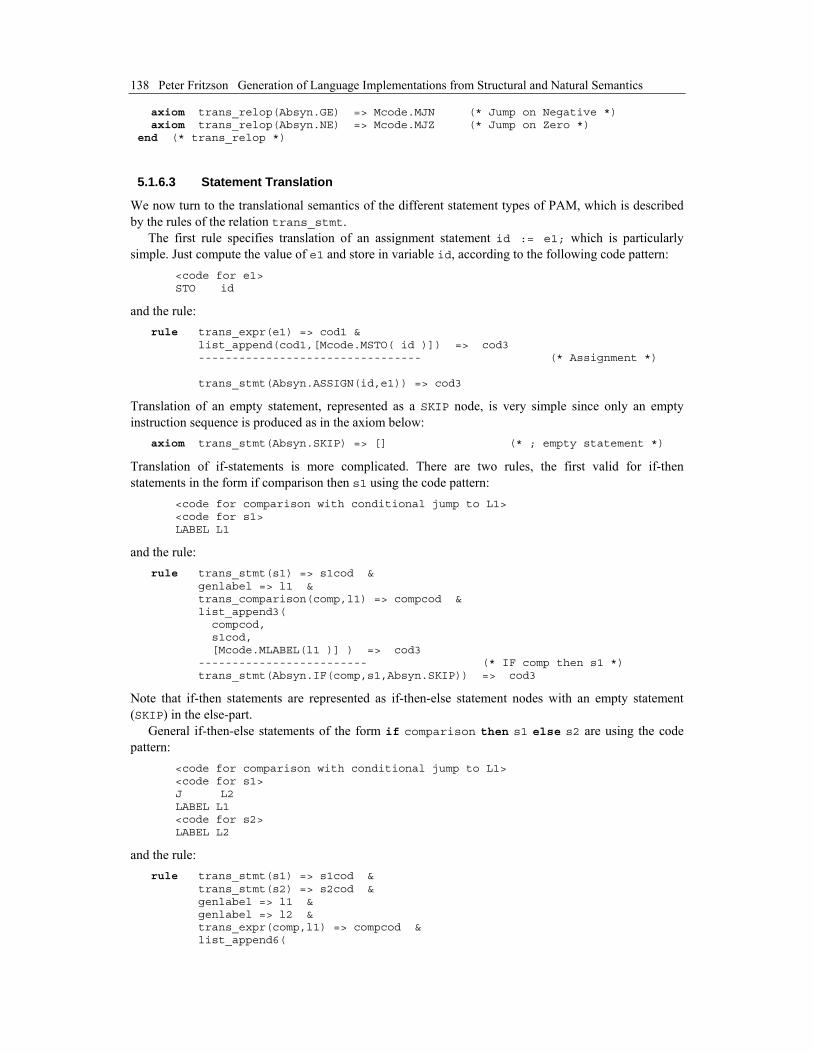
138 Peter Fritzson Generation of Language Implementations from Structural and Natural Semantics
axiom trans_relop(Absyn.GE) => Mcode.MJN (* Jump on Negative *) axiom trans_relop(Absyn.NE) => Mcode.MJZ (* Jump on Zero *) end (* trans_relop *)
5.1.6.3 Statement Translation
We now turn to the translational semantics of the different statement types of PAM, which is described by the rules of the relation trans_stmt.
The first rule specifies translation of an assignment statement id := e1; which is particularly simple. Just compute the value of e1 and store in variable id, according to the following code pattern: <code for e1> STO id
and the rule: rule trans_expr(e1) => cod1 & list_append(cod1,[Mcode.MSTO( id )]) => cod3 --------------------------------- (* Assignment *) trans_stmt(Absyn.ASSIGN(id,e1)) => cod3
Translation of an empty statement, represented as a SKIP node, is very simple since only an empty instruction sequence is produced as in the axiom below: axiom trans_stmt(Absyn.SKIP) => [] (* ; empty statement *)
Translation of if-statements is more complicated. There are two rules, the first valid for if-then statements in the form if comparison then s1 using the code pattern: <code for comparison with conditional jump to L1> <code for s1> LABEL L1
and the rule: rule trans_stmt(s1) => s1cod & genlabel => l1 & trans_comparison(comp,l1) => compcod & list_append3( compcod, s1cod, [Mcode.MLABEL(l1 )] ) => cod3 ------------------------- (* IF comp then s1 *) trans_stmt(Absyn.IF(comp,s1,Absyn.SKIP)) => cod3
Note that if-then statements are represented as if-then-else statement nodes with an empty statement (SKIP) in the else-part.
General if-then-else statements of the form if comparison then s1 else s2 are using the code pattern: <code for comparison with conditional jump to L1> <code for s1> J L2 LABEL L1 <code for s2> LABEL L2
and the rule: rule trans_stmt(s1) => s1cod & trans_stmt(s2) => s2cod & genlabel => l1 & genlabel => l2 & trans_expr(comp,l1) => compcod & list_append6(

Chapter 5 Translational Semantics 139
compcod, s1cod, [Mcode.MJMP( l2 )], [Mcode.MLABEL(l1 )], s2cod, [Mcode.MLABEL(l2 )] ) => cod3 ------------------------- (* if comp then s1 else s2 *) trans_stmt(Absyn.IF(comp,s1,s2)) => cod3
This second rule also specifies correct semantics for if-then statements, although one unnecessary jump instruction would be produced. Avoiding this jump is the only reason for keeping the first rule.
We now turn to while-statements of the form while comparison do s1. This is an iterative statement and thus contain a backward jump in its code-pattern below: LABEL L1 <code for comparison, including conditional jump to L2> <code for s1> J L1 LABEL L2
with the rule: rule trans_stmt(s1) => bodycod & genlabel => l1 & genlabel => l2 & trans_comparison(comp,l2) => compcod & list_append5( [Mcode.MLABEL( l1 )], compcod, bodycod, [Mcode.MJMP( l1 )], [Mcode.MLABEL( l2 )] ) => cod3 --------------------------------------- (* WHILE ... *) trans_stmt(Absyn.WHILE(comp,s1)) => cod3
The definite loop statement of the form to e1 do s1 is a kind of for-statement that found in many other languages. The statement s1 is executed the number of times specified by evaluating expression e1 once at the beginning of its execution. The value of e1 initializes a temporary counter variable which is decremented before each iteration. The loop is exited when the counter becomes negative. The code pattern follows below: <code for e1> STO T1 (* T1 is the counter *) LABEL L1 LOAD T1 SUB 1 (* Decrement T1 *) JN L2 (* Exit the loop *) STO T1 <code for s1> J L1 LABEL L2
and the rule: rule trans_expr(e1) => tocod & trans_stmt(s1) => bodycod & gentemp => t1 & genlabel => l1 & genlabel => l2 & list_append10( tocod, [Mcode.MSTO( t1 )], [Mcode.MLABEL( l1 )], [Mcode.MLOAD( t1 )], [Mcode.MB(Mcode.MSUB, N(1))], [Mcode.MJ(Mcode.MJN, l2)],
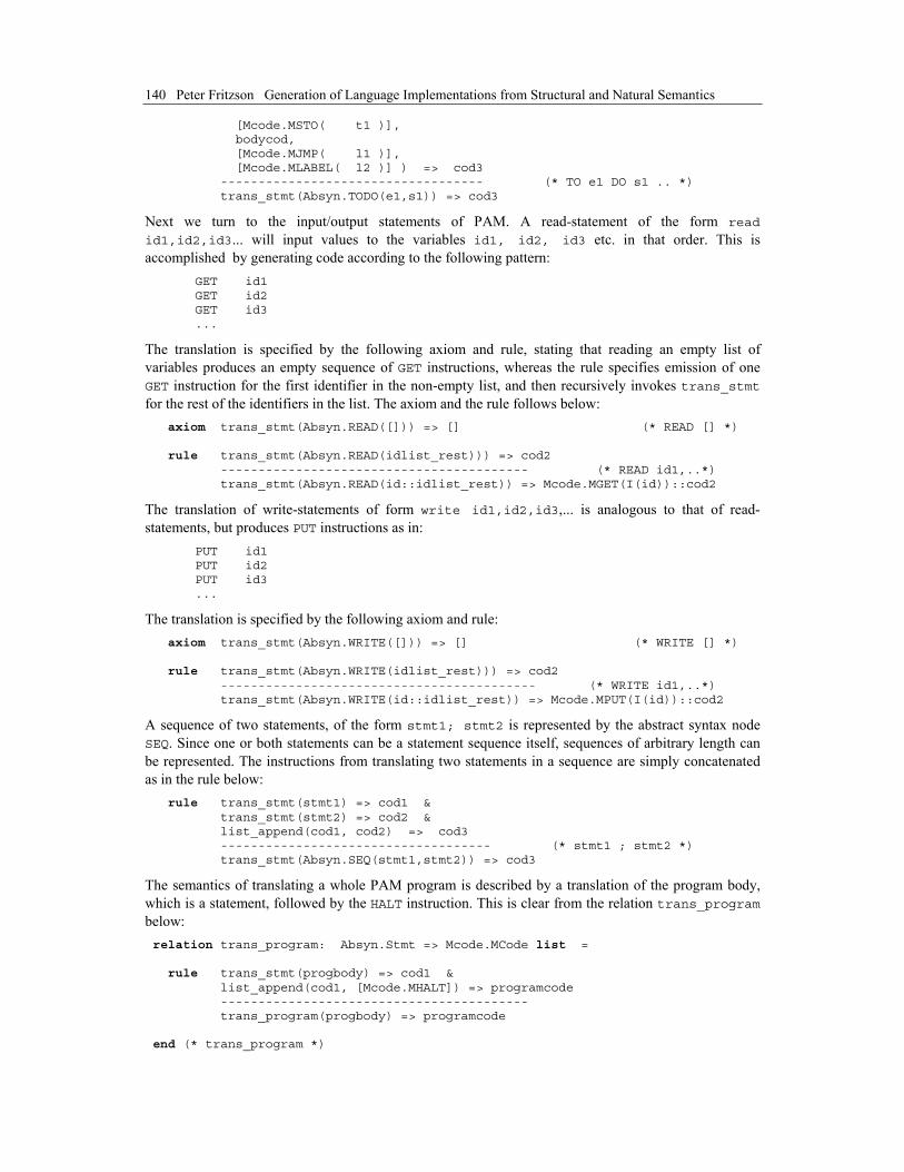
140 Peter Fritzson Generation of Language Implementations from Structural and Natural Semantics
[Mcode.MSTO( t1 )], bodycod, [Mcode.MJMP( l1 )], [Mcode.MLABEL( l2 )] ) => cod3 ----------------------------------- (* TO e1 DO s1 .. *) trans_stmt(Absyn.TODO(e1,s1)) => cod3
Next we turn to the input/output statements of PAM. A read-statement of the form read id1,id2,id3... will input values to the variables id1, id2, id3 etc. in that order. This is accomplished by generating code according to the following pattern: GET id1 GET id2 GET id3 ...
The translation is specified by the following axiom and rule, stating that reading an empty list of variables produces an empty sequence of GET instructions, whereas the rule specifies emission of one GET instruction for the first identifier in the non-empty list, and then recursively invokes trans_stmt for the rest of the identifiers in the list. The axiom and the rule follows below: axiom trans_stmt(Absyn.READ([])) => [] (* READ [] *) rule trans_stmt(Absyn.READ(idlist_rest))) => cod2 ----------------------------------------- (* READ id1,..*) trans_stmt(Absyn.READ(id::idlist_rest)) => Mcode.MGET(I(id))::cod2
The translation of write-statements of form write id1,id2,id3,... is analogous to that of read-statements, but produces PUT instructions as in: PUT id1 PUT id2 PUT id3 ...
The translation is specified by the following axiom and rule: axiom trans_stmt(Absyn.WRITE([])) => [] (* WRITE [] *) rule trans_stmt(Absyn.WRITE(idlist_rest))) => cod2 ------------------------------------------ (* WRITE id1,..*) trans_stmt(Absyn.WRITE(id::idlist_rest)) => Mcode.MPUT(I(id))::cod2
A sequence of two statements, of the form stmt1; stmt2 is represented by the abstract syntax node SEQ. Since one or both statements can be a statement sequence itself, sequences of arbitrary length can be represented. The instructions from translating two statements in a sequence are simply concatenated as in the rule below: rule trans_stmt(stmt1) => cod1 & trans_stmt(stmt2) => cod2 & list_append(cod1, cod2) => cod3 ------------------------------------ (* stmt1 ; stmt2 *) trans_stmt(Absyn.SEQ(stmt1,stmt2)) => cod3
The semantics of translating a whole PAM program is described by a translation of the program body, which is a statement, followed by the HALT instruction. This is clear from the relation trans_program below: relation trans_program: Absyn.Stmt => Mcode.MCode list = rule trans_stmt(progbody) => cod1 & list_append(cod1, [Mcode.MHALT]) => programcode ----------------------------------------- trans_program(progbody) => programcode end (* trans_program *)

Chapter 5 Translational Semantics 141
Finally, the complete translational semantics of PAM statements is presented below as the rules and axioms of the relation trans_stmt.
(*************** Statement translation **************) relation trans_stmt: (Absyn.Stmt) => Mcode.MCode list = (* Statement translation: map the current state into a new state *) rule trans_expr(e1) => cod1 & list_append(cod1, [Mcode.MSTO( Mcode.I(id) )] ) => cod2 ------------------------- (* Assignment *) trans_stmt(Absyn.ASSIGN(id,e1)) => cod2 axiom trans_stmt(Absyn.SKIP) => [] (* ; empty statement *) rule trans_stmt(s1) => s1cod & genlabel => l1 & trans_comparison(comp,l1) => compcod & list_append3( compcod, s1cod, [Mcode.MLABEL(l1 )] ) => cod3 --------------------------- (* if comp then s1 *) trans_stmt(Absyn.IF(comp,s1,Absyn.SKIP)) => cod3 rule trans_stmt(s1) => s1cod & trans_stmt(s2) => s2cod & genlabel => l1 & genlabel => l2 & trans_comparison(comp,l1) => compcod & list_append6( compcod, s1cod, [Mcode.MJMP( l2 )], [Mcode.MLABEL(l1 )], s2cod, [Mcode.MLABEL(l2 )] ) => cod3 --------------------------- (* IF comp then s1 else s2 *) trans_stmt(Absyn.IF(comp,s1,s2)) => cod3 rule trans_stmt(s1) => bodycod & genlabel => l1 & genlabel => l2 & trans_comparison(comp,l2) => compcod & list_append5( [Mcode.MLABEL( l1 )], compcod, bodycod, [Mcode.MJMP( l1 )], [Mcode.MLABEL( l2 )] ) => cod3 --------------------------------------- (* WHILE ... *) trans_stmt(Absyn.WHILE(comp,s1)) => cod3 rule trans_expr(e1) => tocod & trans_stmt(s1) => bodycod & gentemp => t1 & genlabel => l1 & genlabel => l2 & list_append10( tocod, [Mcode.MSTO( t1 )], [Mcode.MLABEL( l1 )], [Mcode.MLOAD( t1 )], [Mcode.MB(Mcode.MSUB, Mcode.N(1))],

142 Peter Fritzson Generation of Language Implementations from Structural and Natural Semantics
[Mcode.MJ(Mcode.MJN, l2)], [Mcode.MSTO( t1 )], bodycod, [Mcode.MJMP( l1 )], [Mcode.MLABEL( l2 )] ) => cod3 ----------------------------------- (* TO e1 DO s1 .. *) trans_stmt(Absyn.TODO(e1,s1)) => cod3 axiom trans_stmt(Absyn.READ([])) => [] (* READ [] *) rule trans_stmt(Absyn.READ(idlist_rest)) => cod2 ----------------------------------------- (* READ id1,..*) trans_stmt(Absyn.READ(id::idlist_rest)) => Mcode.MGET(Mcode.I(id))::cod2 axiom trans_stmt(Absyn.WRITE([])) => [] (* WRITE [] *) rule trans_stmt(Absyn.WRITE(idlist_rest)) => cod2 ------------------------------------------ (* WRITE id1,..*) trans_stmt(Absyn.WRITE(id::idlist_rest)) => Mcode.MPUT(Mcode.I(id))::cod2 rule trans_stmt(stmt1) => cod1 & trans_stmt(stmt2) => cod2 & list_append(cod1, cod2) => cod3 -------------------------------- (* stmt1 ; stmt2 *) trans_stmt(Absyn.SEQ(stmt1,stmt2)) => cod3 end (* trans_stmt *)
5.1.6.4 Emission of Textual Assembly Code
The translational semantics of PAM is specified as a translation from abstract syntax to a sequence of machine instructions in the structured Mcode representation. However, we would like to emit the machine instructions in a textual assembly form. The conversion from the MCode representation to the textual assembly form is accomplished by the emit_assembly function and associated functions below. This is not really part of the translational semantics of RML. Here, RML is used as a semi-functional programming language, to implement the desired conversion. The print primitive has been included in the standard RML library for such purposes. relation emit_assembly: Mcode.MCode list => () = (* Print out the Mcode in textual assembly format * Note: this is not really part of the specification of PAM semantics *) axiom emit_assembly([]) => () rule emit_instr(instr) & emit_assembly(rest) -------------------------- emit_assembly(instr::rest) end (* emit_assembly *) relation emit_instr: Mcode.MCode => () = (* Print an MCode instruction *) rule mbinop_to_str(mbinop) => op & emit_op_operand(op, mopr) -------------------------------------------- emit_instr(Mcode.MB(mbinop, mopr))
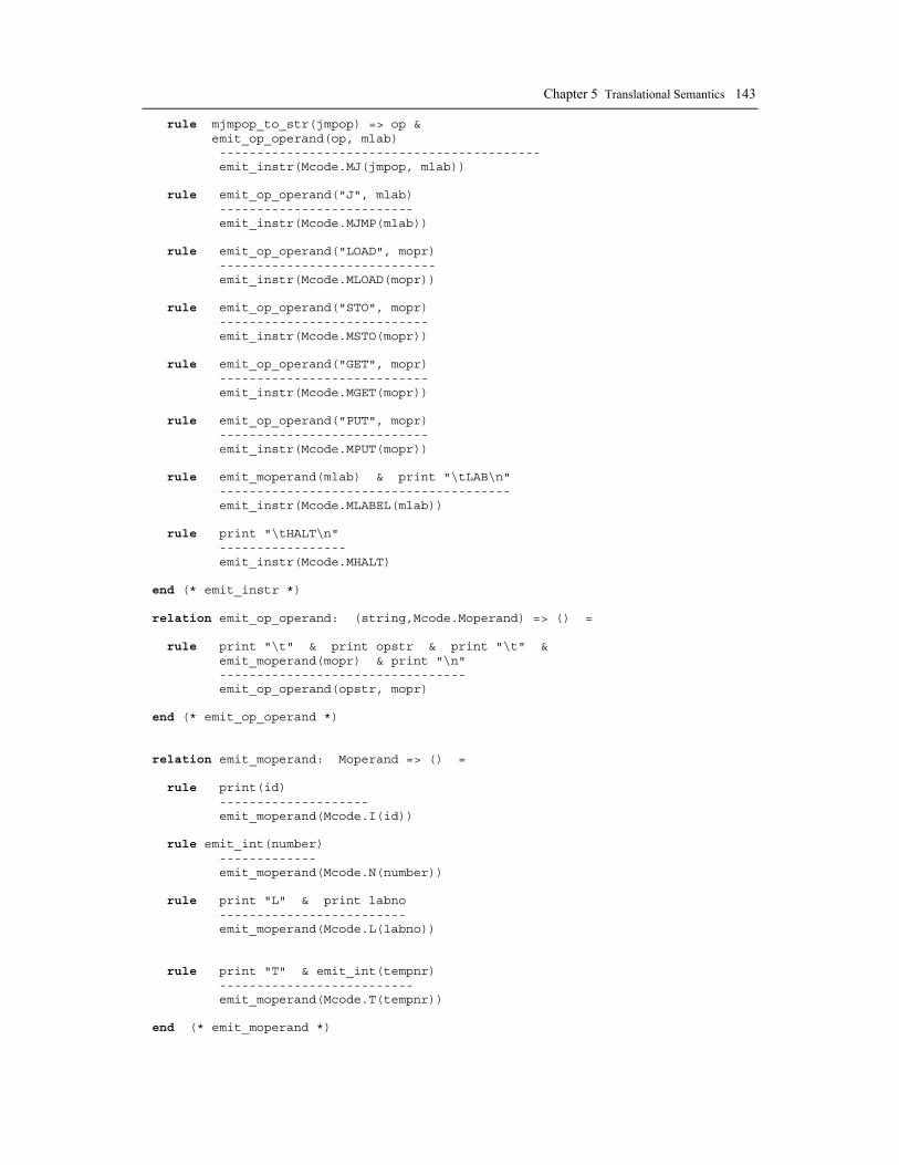
Chapter 5 Translational Semantics 143
rule mjmpop_to_str(jmpop) => op & emit_op_operand(op, mlab) ------------------------------------------- emit_instr(Mcode.MJ(jmpop, mlab)) rule emit_op_operand("J", mlab) -------------------------- emit_instr(Mcode.MJMP(mlab)) rule emit_op_operand("LOAD", mopr) ----------------------------- emit_instr(Mcode.MLOAD(mopr)) rule emit_op_operand("STO", mopr) ---------------------------- emit_instr(Mcode.MSTO(mopr)) rule emit_op_operand("GET", mopr) ---------------------------- emit_instr(Mcode.MGET(mopr)) rule emit_op_operand("PUT", mopr) ---------------------------- emit_instr(Mcode.MPUT(mopr)) rule emit_moperand(mlab) & print "\tLAB\n" --------------------------------------- emit_instr(Mcode.MLABEL(mlab)) rule print "\tHALT\n" ----------------- emit_instr(Mcode.MHALT) end (* emit_instr *) relation emit_op_operand: (string,Mcode.Moperand) => () = rule print "\t" & print opstr & print "\t" & emit_moperand(mopr) & print "\n" --------------------------------- emit_op_operand(opstr, mopr) end (* emit_op_operand *) relation emit_moperand: Moperand => () = rule print(id) -------------------- emit_moperand(Mcode.I(id)) rule emit_int(number) ------------- emit_moperand(Mcode.N(number)) rule print "L" & print labno ------------------------- emit_moperand(Mcode.L(labno)) rule print "T" & emit_int(tempnr) -------------------------- emit_moperand(Mcode.T(tempnr)) end (* emit_moperand *)
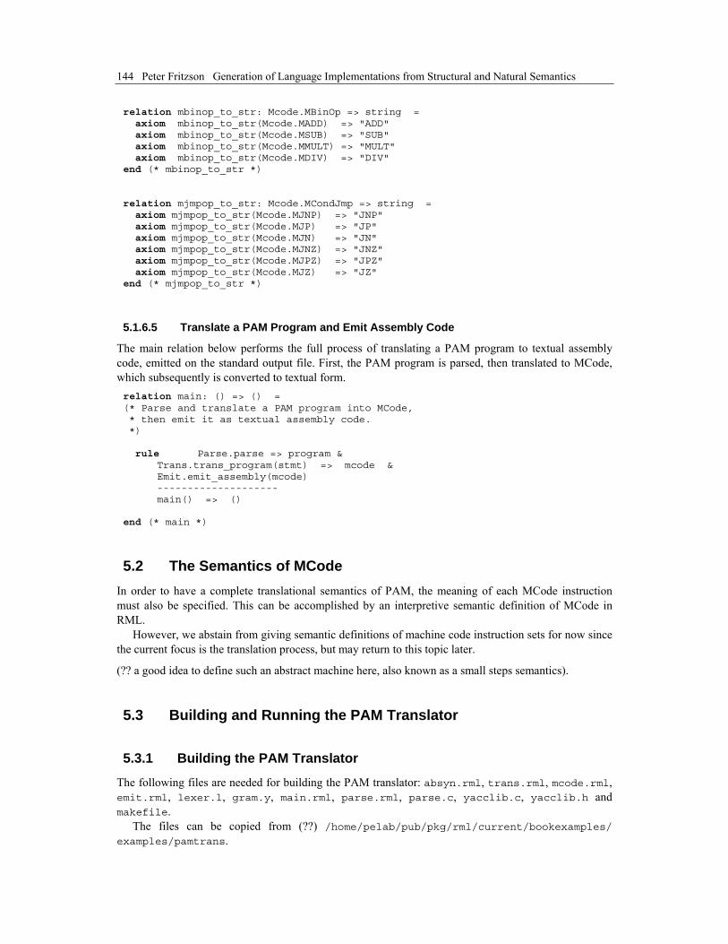
144 Peter Fritzson Generation of Language Implementations from Structural and Natural Semantics
relation mbinop_to_str: Mcode.MBinOp => string = axiom mbinop_to_str(Mcode.MADD) => "ADD" axiom mbinop_to_str(Mcode.MSUB) => "SUB" axiom mbinop_to_str(Mcode.MMULT) => "MULT" axiom mbinop_to_str(Mcode.MDIV) => "DIV" end (* mbinop_to_str *) relation mjmpop_to_str: Mcode.MCondJmp => string = axiom mjmpop_to_str(Mcode.MJNP) => "JNP" axiom mjmpop_to_str(Mcode.MJP) => "JP" axiom mjmpop_to_str(Mcode.MJN) => "JN" axiom mjmpop_to_str(Mcode.MJNZ) => "JNZ" axiom mjmpop_to_str(Mcode.MJPZ) => "JPZ" axiom mjmpop_to_str(Mcode.MJZ) => "JZ" end (* mjmpop_to_str *)
5.1.6.5 Translate a PAM Program and Emit Assembly Code
The main relation below performs the full process of translating a PAM program to textual assembly code, emitted on the standard output file. First, the PAM program is parsed, then translated to MCode, which subsequently is converted to textual form. relation main: () => () = (* Parse and translate a PAM program into MCode, * then emit it as textual assembly code. *) rule Parse.parse => program & Trans.trans_program(stmt) => mcode & Emit.emit_assembly(mcode) -------------------- main() => () end (* main *)
5.2 The Semantics of MCode In order to have a complete translational semantics of PAM, the meaning of each MCode instruction must also be specified. This can be accomplished by an interpretive semantic definition of MCode in RML.
However, we abstain from giving semantic definitions of machine code instruction sets for now since the current focus is the translation process, but may return to this topic later.
(?? a good idea to define such an abstract machine here, also known as a small steps semantics).
5.3 Building and Running the PAM Translator
5.3.1 Building the PAM Translator
The following files are needed for building the PAM translator: absyn.rml, trans.rml, mcode.rml, emit.rml, lexer.l, gram.y, main.rml, parse.rml, parse.c, yacclib.c, yacclib.h and makefile.
The files can be copied from (??) /home/pelab/pub/pkg/rml/current/bookexamples/ examples/pamtrans.

Chapter 5 Translational Semantics 145
The executable is built by typing: sen20%12 make pamtrans
5.3.2 Source Files for PAM Translator lexer.l %{ #include "gram.h" #include "yacclib.h" #include "rml.h" #include "absyn.h" typedef void *rml_t; extern rml_t yylval; int absyn_integer(char *s); int absyn_ident_or_keyword(char *s); %} whitespace [ \t\n]+ letter [a-zA-Z] ident {letter}({letter}|{digit})* digit [0-9] digits {digit}+ icon {digits} /* Lex style lexical syntax of tokens in the PAM language */ %% {whitespace} ; {ident} return absyn_ident_or_keyword(yytext); /* T_IDENT */ {digits} return absyn_integer(yytext); /* T_INTCONST */ ":=" return T_ASSIGN; "+" return T_ADD; "-" return T_SUB; "*" return T_MUL; "/" return T_DIV; "(" return T_LPAREN; ")" return T_RPAREN; "<" return T_LT; "<=" return T_LE; "=" return T_EQ; "<>" return T_NE; ">=" return T_GE; ">" return T_GT; ";" return T_SEMIC; %% /* Make an RML integer from a C string representation (decimal), box it for our abstract syntax, put in yylval and return constant token. */ int absyn_integer(char *s) { yylval=(rml_t) Absyn__INT(mk_icon(atoi(s))); return T_INTCONST; } /* Make an RML Ident or a keyword token from a C string */ /* Reserved words: if,then,else,endif,while,do,end,to,read,write */ static struct keyword_s

146 Peter Fritzson Generation of Language Implementations from Structural and Natural Semantics
{ char *name; int token; } kw[] = { {"do", T_DO}, {"else", T_ELSE}, {"end", T_END}, {"if", T_IF}, {"read", T_READ}, {"then", T_THEN}, {"while", T_WHILE}, {"write", T_WRITE}, }; int absyn_ident_or_keyword(char *s) { int low = 0; int high = (sizeof kw) / sizeof(struct keyword_s) - 1; while( low <= high ) { int mid = (low + high) / 2; int cmp = strcmp(kw[mid].name, yytext); if( cmp == 0 ) { return kw[mid].token; } else if( cmp < 0 ) low = mid + 1; else high = mid - 1; } yylval = (rml_t) mk_scon(s); return T_IDENT; } gram.y %{ #include <stdio.h> #include "yacclib.h" #include "rml.h" #include "absyn.h" typedef void *rml_t; #define YYSTYPE rml_t extern rml_t absyntree; %} %token T_READ %token T_WRITE %token T_ASSIGN %token T_IF %token T_THEN %token T_ENDIF %token T_ELSE %token T_TO %token T_DO %token T_END %token T_WHILE %token T_LPAREN %token T_RPAREN %token T_IDENT %token T_INTCONST %token T_EQ

Chapter 5 Translational Semantics 147
%token T_LE %token T_LT %token T_GT %token T_GE %token T_NE %token T_ADD %token T_SUB %token T_MUL %token T_DIV %token T_SEMIC %% /* Yacc BNF grammar of the PAM language */ program : series { absyntree = $1; } series : statement { $$ = Absyn__SEQ($1, Absyn__SKIP); } | statement series { $$ = Absyn__SEQ($1, $2); } statement : input_statement T_SEMIC { $$ = $1; } | output_statement T_SEMIC { $$ = $1; } | assignment_statement T_SEMIC { $$ = $1; } | conditional_statement { $$ = $1; } | definite_loop { $$ = $1; } | while_loop { $$ = $1; } input_statement : T_READ variable_list { $$ = Absyn__READ($2); } output_statement : T_WRITE variable_list { $$ = Absyn__WRITE($2); } variable_list : variable { $$ = mk_cons($1, mk_nil()); } | variable variable_list { $$ = mk_cons($1, $2); } assignment_statement : variable T_ASSIGN expression { $$ = Absyn__ASSIGN($1, $3); } conditional_statement : T_IF comparison T_THEN series T_ENDIF { $$ = Absyn__IF($2, $4, Absyn__SKIP); } | T_IF comparison T_THEN series T_ELSE series T_ENDIF { $$ = Absyn__IF($2, $4, $6); } definite_loop : T_TO expression T_DO series T_END { $$ = Absyn__TODO($2, $4); } while_loop : T_WHILE comparison T_DO series T_END { $$ = Absyn__WHILE($2, $4); } expression : term { $$ = $1; } | expression weak_operator term
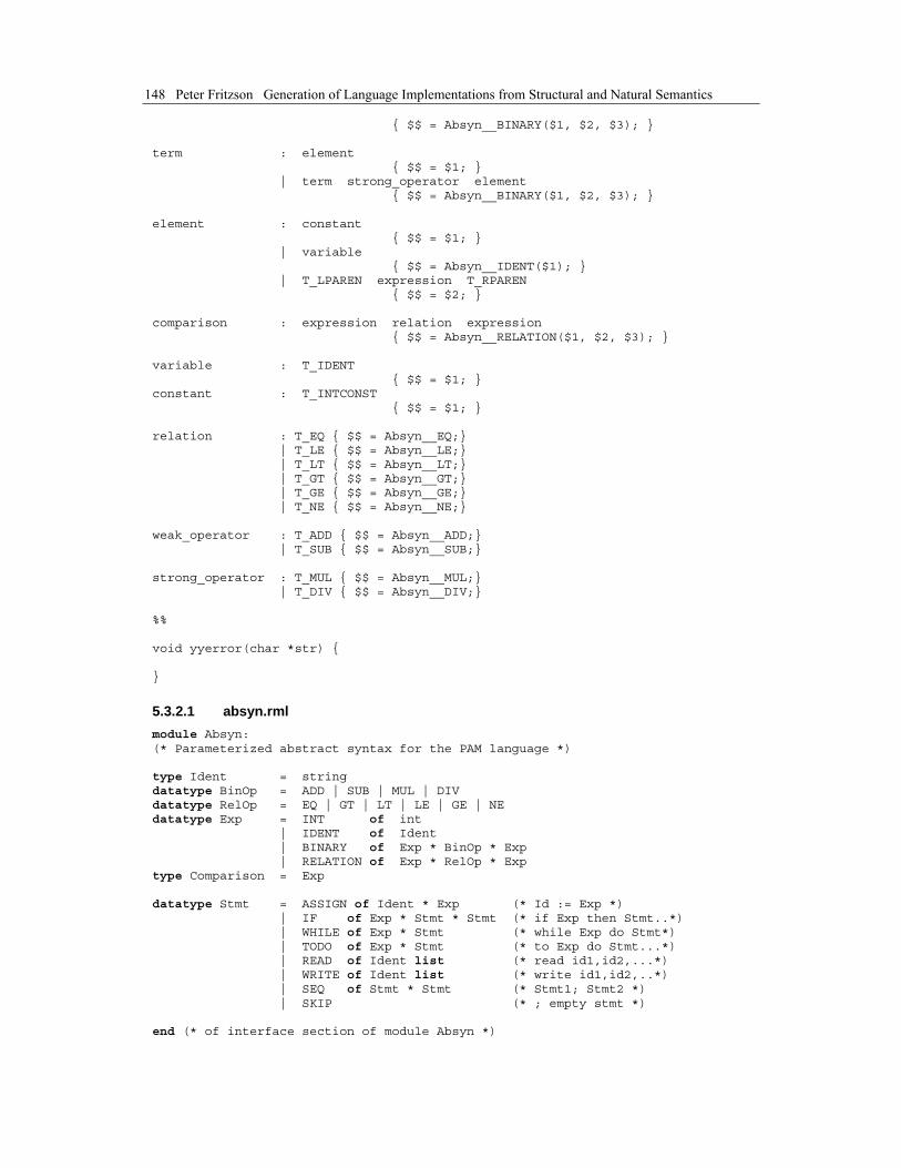
148 Peter Fritzson Generation of Language Implementations from Structural and Natural Semantics
{ $$ = Absyn__BINARY($1, $2, $3); } term : element { $$ = $1; } | term strong_operator element { $$ = Absyn__BINARY($1, $2, $3); } element : constant { $$ = $1; } | variable { $$ = Absyn__IDENT($1); } | T_LPAREN expression T_RPAREN { $$ = $2; } comparison : expression relation expression { $$ = Absyn__RELATION($1, $2, $3); } variable : T_IDENT { $$ = $1; } constant : T_INTCONST { $$ = $1; } relation : T_EQ { $$ = Absyn__EQ;} | T_LE { $$ = Absyn__LE;} | T_LT { $$ = Absyn__LT;} | T_GT { $$ = Absyn__GT;} | T_GE { $$ = Absyn__GE;} | T_NE { $$ = Absyn__NE;} weak_operator : T_ADD { $$ = Absyn__ADD;} | T_SUB { $$ = Absyn__SUB;} strong_operator : T_MUL { $$ = Absyn__MUL;} | T_DIV { $$ = Absyn__DIV;} %% void yyerror(char *str) { }
5.3.2.1 absyn.rml module Absyn: (* Parameterized abstract syntax for the PAM language *) type Ident = string datatype BinOp = ADD | SUB | MUL | DIV datatype RelOp = EQ | GT | LT | LE | GE | NE datatype Exp = INT of int | IDENT of Ident | BINARY of Exp * BinOp * Exp | RELATION of Exp * RelOp * Exp type Comparison = Exp datatype Stmt = ASSIGN of Ident * Exp (* Id := Exp *) | IF of Exp * Stmt * Stmt (* if Exp then Stmt..*) | WHILE of Exp * Stmt (* while Exp do Stmt*) | TODO of Exp * Stmt (* to Exp do Stmt...*) | READ of Ident list (* read id1,id2,...*) | WRITE of Ident list (* write id1,id2,..*) | SEQ of Stmt * Stmt (* Stmt1; Stmt2 *) | SKIP (* ; empty stmt *) end (* of interface section of module Absyn *)

Chapter 5 Translational Semantics 149
5.3.2.2 trans.rml module Trans: with "absyn.rml" with "mcode.rml" relation trans_program: Absyn.Stmt => Mcode.MCode list end (*************** Arithmetic expression translation **************) relation trans_expr: Absyn.Exp => Mcode.MCode list = (* Evaluation of expressions in the current environment *) axiom trans_expr(Absyn.INT(v)) => [Mcode.MLOAD( Mcode.N(v))] (* integer constant *) axiom trans_expr(Absyn.IDENT(id)) => [Mcode.MLOAD( Mcode.I(id))] (* identifier id *) (* Arith binop: simple case, expr2 is just an identifier or constant *) rule trans_expr(e1) => cod1 & trans_expr(e2) => [Mcode.MLOAD(operand2)] & (* expr2 simple *) trans_binop(binop) => opcode & list_append(cod1, [Mcode.MB(opcode,operand2)]) => cod3 ----------------------------------- (* expr1 binop expr2 *) trans_expr(Absyn.BINARY(e1,binop,e2)) => cod3 (* Arith binop: general case, expr2 is a more complicated expr *) rule trans_expr(e1) => cod1 & trans_expr(e2) => cod2 & trans_binop(binop) => opcode & gentemp => t1 & gentemp => t2 & list_append6( cod1, (* code for expr1 *) [Mcode.MSTO(t1)], (* store expr1 *) cod2, (* code for expr2 *) [Mcode.MSTO(t2)], (* store expr2 *) [Mcode.MLOAD(t1)], (* load expr1 value into Acc *) [Mcode.MB(opcode,t2)] ) => cod3 (* Do arith operation *) ----------------------------------- (* expr1 binop expr2 *) trans_expr(Absyn.BINARY(e1,binop,e2)) => cod3 end (* trans_expr *) relation trans_binop: Absyn.BinOp => Mcode.MBinOp = axiom trans_binop(Absyn.ADD) => Mcode.MADD axiom trans_binop(Absyn.SUB) => Mcode.MSUB axiom trans_binop(Absyn.MUL) => Mcode.MMULT axiom trans_binop(Absyn.DIV) => Mcode.MDIV end relation gentemp: () => Mcode.MOperand = rule tick => no ---------- gentemp => Mcode.T(no) end (* gentemp *) relation genlabel: () => Mcode.MOperand =
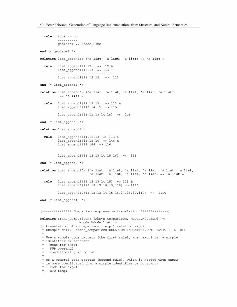
150 Peter Fritzson Generation of Language Implementations from Structural and Natural Semantics
rule tick => no ---------- genlabel => Mcode.L(no) end (* genlabel *) relation list_append3: ('a list, 'a list, 'a list) => 'a list = rule list_append(l1,l2) => l12 & list_append(l12,l3) => l13 ---------------------------- list_append3(l1,l2,l3) => l13 end (* list_append3 *) relation list_append5: ('a list, 'a list, 'a list, 'a list, 'a list) => 'a list = rule list_append3(l1,l2,l3) => l13 & list_append3(l13,l4,l5) => l15 ---------------------------- list_append5(l1,l2,l3,l4,l5) => l15 end (* list_append5 *) relation list_append6 = rule list_append3(l1,l2,l3) => l13 & list_append3(l4,l5,l6) => l46 & list_append(l13,l46) => l16 ------------------------------- list_append6(l1,l2,l3,l4,l5,l6) => l16 end (* list_append6 *) relation list_append10: ('a list, 'a list, 'a list, 'a list, 'a list, 'a list, 'a list, 'a list, 'a list, 'a list) => 'a list = rule list_append5(l1,l2,l3,l4,l5) => l15 & list_append6(l15,l6,l7,l8,l9,l10) => l110 ---------------------------- list_append10(l1,l2,l3,l4,l5,l6,l7,l8,l9,l10) => l110 end (* list_append10 *) (*************** Comparison expression translation **************) relation trans_comparison: (Absyn.Comparison, Mcode.MOperand) => Mcode.MCode list = (* translation of a comparison: expr1 relation expr2 * Example call: trans_comparison(RELATION(INDENT(x), GT, INT(5)), L(10)) * * Use a simple code pattern (the first rule), when expr2 is a simple * identifier or constant: * code for expr1 * SUB operand2 * conditional jump to lab * * or a general code pattern (second rule), which is needed when expr2 * is more complicated than a simple identifier or constant: * code for expr1 * STO temp1

Chapter 5 Translational Semantics 151
* code for expr2 * SUB temp1 * conditional jump to lab *) rule trans_expr(e1) => cod1 & trans_expr(e2) => [Mcode.MLOAD(operand2)] & trans_relop(relop) => jmpop & list_append3( cod1, [Mcode.MB(Mcode.MSUB, operand2)], [Mcode.MJ(jmpop,lab)] ) => cod3 ----------------------------------- (* expr1 relop expr2 *) trans_comparison(Absyn.RELATION(e1,relop,e2),lab) => cod3 rule trans_expr(e1) => cod1 & trans_expr(e2) => cod2 & trans_relop(relop) => jmpop & gentemp => t1 & list_append5( cod1, [Mcode.MSTO(t1)], cod2, [Mcode.MB(Mcode.MSUB,t1)], [Mcode.MJ(jmpop,lab)] ) => cod3 ----------------------------------- (* expr1 relop expr2 *) trans_comparison(Absyn.RELATION(e1,relop,e2),lab) => cod3 end (* trans_comparison *) relation trans_relop: Absyn.RelOp => Mcode.MCondJmp = (* Note that for these relational operators, the selected jump * instruction is logically opposite. For example, if equality to zero * is true, we should should just continue, otherwise jump (MJNP) *) axiom trans_relop(Absyn.EQ) => Mcode.MJNP (* Jump on Negative or Positive *) axiom trans_relop(Absyn.LE) => Mcode.MJP (* Jump on Positive *) axiom trans_relop(Absyn.LT) => Mcode.MJPZ (* Jump on Positive or Zero *) axiom trans_relop(Absyn.GT) => Mcode.MJNZ (* Jump on Negative or Zero *) axiom trans_relop(Absyn.GE) => Mcode.MJN (* Jump on Negative *) axiom trans_relop(Absyn.NE) => Mcode.MJZ (* Jump on Zero *) end (* trans_relop *) (*************** Statement translation **************) relation trans_stmt: (Absyn.Stmt) => Mcode.MCode list = (* Statement translation: map the current state into a new state *) (* correct?? *) rule trans_expr(e1) => cod1 & list_append(cod1, [Mcode.MSTO( Mcode.I(id) )] ) => cod2 ------------------------- (* Assignment *) trans_stmt(Absyn.ASSIGN(id,e1)) => cod2 axiom trans_stmt(Absyn.SKIP) => [] (* ; empty statement *) rule trans_stmt(s1) => s1cod & genlabel => l1 & trans_comparison(comp,l1) => compcod & list_append3( compcod, s1cod,
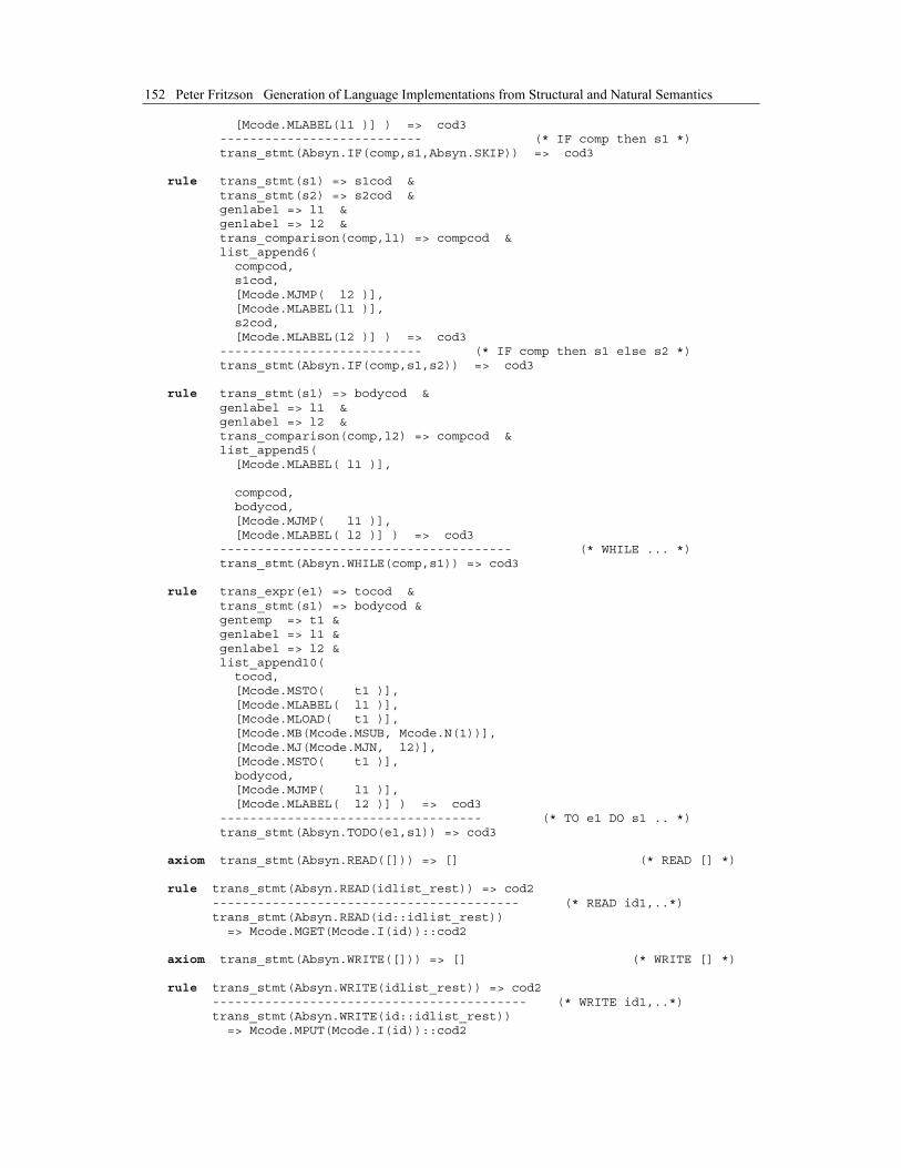
152 Peter Fritzson Generation of Language Implementations from Structural and Natural Semantics
[Mcode.MLABEL(l1 )] ) => cod3 --------------------------- (* IF comp then s1 *) trans_stmt(Absyn.IF(comp,s1,Absyn.SKIP)) => cod3 rule trans_stmt(s1) => s1cod & trans_stmt(s2) => s2cod & genlabel => l1 & genlabel => l2 & trans_comparison(comp,l1) => compcod & list_append6( compcod, s1cod, [Mcode.MJMP( l2 )], [Mcode.MLABEL(l1 )], s2cod, [Mcode.MLABEL(l2 )] ) => cod3 --------------------------- (* IF comp then s1 else s2 *) trans_stmt(Absyn.IF(comp,s1,s2)) => cod3 rule trans_stmt(s1) => bodycod & genlabel => l1 & genlabel => l2 & trans_comparison(comp,l2) => compcod & list_append5( [Mcode.MLABEL( l1 )], compcod, bodycod, [Mcode.MJMP( l1 )], [Mcode.MLABEL( l2 )] ) => cod3 --------------------------------------- (* WHILE ... *) trans_stmt(Absyn.WHILE(comp,s1)) => cod3 rule trans_expr(e1) => tocod & trans_stmt(s1) => bodycod & gentemp => t1 & genlabel => l1 & genlabel => l2 & list_append10( tocod, [Mcode.MSTO( t1 )], [Mcode.MLABEL( l1 )], [Mcode.MLOAD( t1 )], [Mcode.MB(Mcode.MSUB, Mcode.N(1))], [Mcode.MJ(Mcode.MJN, l2)], [Mcode.MSTO( t1 )], bodycod, [Mcode.MJMP( l1 )], [Mcode.MLABEL( l2 )] ) => cod3 ----------------------------------- (* TO e1 DO s1 .. *) trans_stmt(Absyn.TODO(e1,s1)) => cod3 axiom trans_stmt(Absyn.READ([])) => [] (* READ [] *) rule trans_stmt(Absyn.READ(idlist_rest)) => cod2 ----------------------------------------- (* READ id1,..*) trans_stmt(Absyn.READ(id::idlist_rest)) => Mcode.MGET(Mcode.I(id))::cod2 axiom trans_stmt(Absyn.WRITE([])) => [] (* WRITE [] *) rule trans_stmt(Absyn.WRITE(idlist_rest)) => cod2 ------------------------------------------ (* WRITE id1,..*) trans_stmt(Absyn.WRITE(id::idlist_rest)) => Mcode.MPUT(Mcode.I(id))::cod2

Chapter 5 Translational Semantics 153
rule trans_stmt(stmt1) => cod1 & trans_stmt(stmt2) => cod2 & list_append(cod1, cod2) => cod3 -------------------------------- (* stmt1 ; stmt2 *) trans_stmt(Absyn.SEQ(stmt1,stmt2)) => cod3 end (* trans_stmt *) relation trans_program: Absyn.Stmt => Mcode.MCode list = rule trans_stmt(progbody) => cod1 & list_append(cod1, [Mcode.MHALT]) => programcode ----------------------------------------- trans_program(progbody) => programcode end (* trans_program *)
5.3.2.3 mcode.rml module Mcode: type Id = string datatype MBinOp = MADD | MSUB | MMULT | MDIV datatype MCondJmp = MJNP | MJP | MJN | MJNZ | MJPZ | MJZ datatype MOperand = I of Id | N of int | T of int | L of int (*datatype MLab = L of int type MTemp = T of int type MIdent = I of Id type MIdTemp = I of Id | T of int *) datatype MCode = MB of MBinOp * MOperand (* Binary arith ops *) | MJ of MCondJmp * MOperand (* Conditional jumps *) | MJMP of MOperand | MLOAD of MOperand | MSTO of MOperand | MGET of MOperand | MPUT of MOperand | MLABEL of MOperand | MHALT end
5.3.2.4 emit.rml module Emit: with "mcode.rml" relation emit_assembly: Mcode.MCode list => () end relation emit_assembly: Mcode.MCode list => () = (* Print out the MCode in textual assembly format * Note: this is not really part of the specification of PAM semantics *) axiom emit_assembly([]) => () rule emit_instr(instr) & emit_assembly(rest) -------------------------- emit_assembly(instr::rest)

154 Peter Fritzson Generation of Language Implementations from Structural and Natural Semantics
end (* emit_assembly *) relation emit_instr: Mcode.MCode => () = (* Print an MCode instruction *) rule mbinop_to_str(mbinop) => op & emit_op_operand(op, mopr) -------------------------------------------- emit_instr(Mcode.MB(mbinop, mopr)) rule mjmpop_to_str(jmpop) => op & emit_op_operand(op, mlab) ------------------------------------------- emit_instr(Mcode.MJ(jmpop, mlab)) rule emit_op_operand("J", mlab) -------------------------- emit_instr(Mcode.MJMP(mlab)) rule emit_op_operand("LOAD", mopr) ----------------------------- emit_instr(Mcode.MLOAD(mopr)) rule emit_op_operand("STO", mopr) ---------------------------- emit_instr(Mcode.MSTO(mopr)) rule emit_op_operand("GET", mopr) ---------------------------- emit_instr(Mcode.MGET(mopr)) rule emit_op_operand("PUT", mopr) ---------------------------- emit_instr(Mcode.MPUT(mopr)) rule emit_moperand(mlab) & print "\tLAB\n" --------------------------------------- emit_instr(Mcode.MLABEL(mlab)) rule print "\tHALT\n" ----------------- emit_instr(Mcode.MHALT) end (* emit_instr *) relation emit_op_operand: (string,Mcode.MOperand) => () = rule print "\t" & print opstr & print "\t" & emit_moperand(mopr) & print "\n" --------------------------------- emit_op_operand(opstr, mopr) end (* emit_op_operand *) relation emit_int: int => () = rule int_string(i) => s & print s --------- emit_int(i) end

Chapter 5 Translational Semantics 155
relation emit_moperand: Mcode.MOperand => () = rule print(id) -------------------- emit_moperand(Mcode.I(id)) rule emit_int(number) ------------- emit_moperand(Mcode.N(number)) rule print "L" & emit_int(labno) ------------------------- emit_moperand(Mcode.L(labno)) rule print "T" & emit_int(tempnr) -------------------------- emit_moperand(Mcode.T(tempnr)) end (* emit_moperand *) relation mbinop_to_str: Mcode.MBinOp => string = axiom mbinop_to_str(Mcode.MADD) => "ADD" axiom mbinop_to_str(Mcode.MSUB) => "SUB" axiom mbinop_to_str(Mcode.MMULT) => "MULT" axiom mbinop_to_str(Mcode.MDIV) => "DIV" end (* mbinop_to_str *) relation mjmpop_to_str: Mcode.MCondJmp => string = axiom mjmpop_to_str(Mcode.MJNP) => "JNP" axiom mjmpop_to_str(Mcode.MJP) => "JP" axiom mjmpop_to_str(Mcode.MJN) => "JN" axiom mjmpop_to_str(Mcode.MJNZ) => "JNZ" axiom mjmpop_to_str(Mcode.MJPZ) => "JPZ" axiom mjmpop_to_str(Mcode.MJZ) => "JZ" end (* mjmpop_to_str *)
5.3.2.5 main.rml module Main: relation main: () => () end with "parse.rml" with "trans.rml" with "emit.rml" relation main: () => () = (* Parse and translate a PAM program into MCode, * then emit it as textual assembly code. *) rule Parse.parse() => program & Trans.trans_program(program) => mcode & Emit.emit_assembly(mcode) -------------------- main end (* main *)
5.3.2.6 parse.rml module Parse:

156 Peter Fritzson Generation of Language Implementations from Structural and Natural Semantics
with "absyn.rml" relation parse: () => Absyn.Stmt end parse.c #include <stdio.h> #include <errno.h> #include <string.h> #include "rml.h" #ifndef RML_INSPECTBOX #define RML_INSPECTBOX(d,h,p) (RML_ISIMM((d)=(p))?0:(((h)=(void*)RML_GETHDR((p))),0)) #define rml_prim_deref_imm(x) x #endif void Parse_5finit(void) {} void *absyntree; RML_BEGIN_LABEL(Parse__parse) { void *a0, *a0hdr; RML_INSPECTBOX(a0, a0hdr, rmlA0); if( a0hdr == RML_IMMEDIATE(RML_UNBOUNDHDR) ) RML_TAILCALLK(rmlFC); else { if(yyparse()==0) { rmlA0 = absyntree; RML_TAILCALLK(rmlSC); } else RML_TAILCALLK(rmlFC); } } makefile # Makefile for building translational version of PAM # # ??Note: LDFLAGS, CFLAGS are non-portable for some Unix systems # VARIABLES SHELL = /bin/sh LDLIBS = -lrml -ll # Order is essential; we want librml main, not libll! LDFLAGS = -L$(RMLRUNTIME)/lib/plain/ CC = gcc CFLAGS = -I$(RMLRUNTIME)/include/plain/ -g -I.. RML2C = $(RMLRUNTIME)/bin/rml2c # EVERYTHING all: pamtrans # EXECUTABLE COMMONOBJS=yacclib.o VSLOBJS=main.o lexer.o gram.o parse.o absyn.o mcode.o trans.o emit.o pamtrans: $(VSLOBJS) $(COMMONOBJS) $(CC) $(LDFLAGS) $(VSLOBJS) $(COMMONOBJS) $(LDLIBS) -o pamtrans # MAIN ROUTINE WRITTEN IN RML NOW main.o: main.c main.c main.h: main.rml $(RML2C) -c main.rml

Chapter 5 Translational Semantics 157
# YACCLIB yacclib.o: yacclib.c $(CC) $(CFLAGS) -c -o yacclib.o yacclib.c # LEXER lexer.o: lexer.c gram.h absyn.h lexer.c: lexer.l lex -t lexer.l >lexer.c # PARSER gram.o: gram.c gram.h gram.c gram.h: gram.y yacc -d gram.y mv y.tab.c gram.c mv y.tab.h gram.h # INTERFACE TO SCANNER/PARSER (RML CALLING C) parse.o: parse.c absyn.h # ABSTRACT SYNTAX absyn.o: absyn.c absyn.c absyn.h: absyn.rml $(RML2C) -c absyn.rml # TRANSLATION trans.o: trans.c trans.c trans.h: trans.rml absyn.h $(RML2C) -c trans.rml # EMISSION emit.o: emit.c emit.c emit.h: emit.rml $(RML2C) -c emit.rml # INTERMEDIATE FORM mcode.o: mcode.c mcode.c mcode.h: mcode.rml $(RML2C) -c mcode.rml # AUX clean: $(RM) pamtrans $(COMMONOBJS) $(VSLOBJS) main.c main.h lexer.c parser.c parser.h absyn.c absyn.h env.c env.h eval.c eval.h *~#include <stdlib.h>
5.4 Summary This chapter introduced the concept of translational semantics, which was applied to the small PAM language. A translational semantics for translating PAM to a simple machine language was developed. The machine has only one register, and includes arithmetic instructions and conditional and unconditional jump instructions. A structured representation of the instruction set, called MCode, was

158 Peter Fritzson Generation of Language Implementations from Structural and Natural Semantics
defined. Much of the translation is expressed through parameterized code templates within some of the RML rules.
The reader may have noted that we used many append instructions in the semantics, since the sequence of output code instructions is represented as a linked list. This can be avoided by an alternative way of representing the output code as an ordered sequence of instructions. For example, we can use a binary tree built by a binary sequencing operator (e.g. MSEQ), which can be obtained by for example adding an MSEQ of MCode * MCode operator declaration to the MCode union type.
For the interested user it can be mentioned that there is yet a third possible formulation of the semantics which avoids using append (although there is nothing wrong in principle with append). Using the so called Continuation Passing Style (CPS) formulation [??ref], the code is built backward starting from the end. Each relation would accept a formal parameter rest, and would add its own code before rest, using the :: (list cell concatenation) operator.
(BRK)

159
Chapter 6 A Large Translational Semantics
The purpose of this chapter is to give an example of a Structured Operational Semantics translational specification of a realistically sized language, and how to structure such a specification. The language in question is called Petrol – a rather strange name, but understandable knowing that its predecessor is called Diesel.
Petrol is a Pascal-like language, with a complexity roughly comparable to Pascal. It has a Pascal-like syntax, allows nested procedures, records and type declarations, pointers, and most of the usual control structures. In addition it adds some features from C, such as pointer arithmetic, array parameters, type casting and a constant 0 which is overloaded for all pointer and numeric types (i.e., it can be used both as nil and as an integer or floating point zero). The reason to include these low level C-like features is to study how they can be described in the specification and integrated with the rest of the Petrol language.
Flattening: Remove nesting
(Expand control structures)
Scanning
Parsing
Text
Token sequence
Abstract syntax (Absyn)
Flattened code (FCode)
Static elaborationType analysis; handle types,
overloading, records, array-indexingTree Code (TCode)
Code emission
Low level C
Figure 6-1. Translational steps of the Petrol compiler. The three last steps are generated from a Structured Operational Semantics specification of Petrol in RML.
The rules of good software engineering practice also applies to specifications of programming languages. A large specification should be structured into modules, each of which should describe clearly defined steps in the translation processes, and with specified interfaces between these steps. We have tried to apply these rules to the specification of Petrol in RML. The size of the complete specification is about 2000 lines spread over 10 modules.
The specified compiler translates Petrol programs to low level C code, which easily could be replaced by some machine code similar to what we used as output from the PAM compiler. However, by using C as output we can conveniently re-use existing highly optimizing C back-ends. This is also a good example of the common technique of implementing a programming language by generating C, sometimes called the universal assembly language.
160 Peter Fritzson Generation of Language Implementations from Structural and Natural Semantics
The scanner and parser modules of the Petrol compiler are generated by Lex and Yacc as usual. Semantic analysis and intermediate code generation is divided into three steps, see Figure 6-1. The reason is to make the specification more modular and understandable, and avoid errors.
The parser produces abstract syntax by calling abstract syntax tree building actions at the reduction of grammar rules. The structure of the abstract syntax is specified by the RML module Absyn.
The first step in the semantic analysis performs static elaborations, such as checking types and definition-before-use together with a number of simplifications of the high-level abstract syntax such as resolving arithmetic operator overloading (the same +,*,- are used for both integers and reals) and array indexing. The output of this step is a simpler representation which is very similar to abstract syntax and called TCode (Tree Code). The semantics of this step is expressed by RML modules static.rml and types.rml.
The next step in semantic analysis performs flattening, i.e., reducing nested scopes of procedures within procedures to a single scope level. The non-local accesses of variables and procedures from within nested scopes can be handled by introducing mechanisms such as a static link or a display. The used representation can be converted to either mechanism. However, in the final code we choose the display, i.e., an array of pointers to procedure activation records. The output of this step is called FCode (flattened code), which still keeps most of the original structure of Petrol expressions. Petrol statements which express complicated control structures could have been reduced to simple goto instructions during this phase. However, since the generated compiler in this case eventually will emit C code, the control structures are kept and translated to corresponding C statements in the final code emission phase.
Finally, the low level FCode (which still is rather similar to TCode) is emitted as C-code, to be compiled and executed. This code emission phase is not declarative, and not really part of the semantic specification of Petrol. For example, it could have been written in C. However, we choose to express also this part in RML, which allows use of the convenient pattern matching facilities and access to the definition of TCode.
6.1 The Petrol Language Before going into details of the semantic specification of Petrol, it is useful to give a brief background information about the Petrol language constructs in order to gain some understanding of the language. A Petrol example, the classical factorial function, follows below: function fact(n : integer) : integer; var temp : integer; begin if n = 0 then return 1 else temp := fact(n - 1); return n * temp; end; end;
6.1.1 Petrol Language Constructs
As already remarked, Petrol is a Pascal-like language with some C-like extensions. An overview of the Petrol language constructs follows below.
6.1.1.1 Petrol Expressions and Operators
The usual Pascal arithmetic operators for integer and real numbers are included. Integer division is performed by div, whereas / always gives a real result. Petrol, just like C, allows expressions of floating

Chapter 6 A Large Translational Semantics 161
point type, character type or pointer type in a boolean context. The expression having a value of zero or nil is interpreted as false; nonzero is true. The arithmetic operators follow below: +, -, *, /, div, mod
Typical arithmetic expressions: 3.14159+x, 2-x*y, number+(x div y)
Relational operators: <, >, <=, >=, <>, =
Logical operators operate on boolean values represented as integers. Character or pointer values are automatically converted before applying these operators: or, and, not
The address-of operator: &, and the dereferencing operator ^ are supported. General address arithmetic as in the C language, is also supported. The null pointer is represented by the predefined identifier nil. ptr := &x; y := x^; z := (ptr+5)^ ptr := nil;
Explicit type casting, i.e., type conversion, is supported between integer and pointer types, between arbitrary pointer types, and between character, integer and real in both directions. Truncation will occur when converting from a wider type (such as int) to a narrower type (such as char). For example, a pointer ptr can be converted to an integer as follows: ivalue := cast(integer,ptr);
The constant 0 can denote either an integer zero or is converted to a real zero depending on the context. The constant 0 does not represent a nil pointer as in C, however. Instead the predefined identifier nil must be used.
6.1.1.2 Petrol Declarations and Types
Some examples of Petrol declarations follow below. The basic types supported by Petrol are integers and reals. Strings only occur as constants. Additional types can be defined using records, arrays and pointers. Functions and procedures can be defined, including external functions/procedures. Argument passing is call-by-value, except for array expressions which are automatically converted to pointer expressions passed by value, just like in C. Thus, for an array argument the address of the array is passed by value—not the array itself. const pi = 3.14; type trec = record a: integer; x: real; end; var x,y: integer; var arr: array [20] of integer; function fib(x : integer) : integer; .... procedure write_int(val : integer); .... function malloc(nbytes : integer) : ^cons_t; extern;
6.1.1.3 Petrol Statement Types
The Petrol statements types are listed below, together with an example of each statement. Assignment: x := a+b; If-then statement: if a=5 then x:= 35; end; If-then-else stmt: if a=6 then x:= 40; else x:= 45; end;
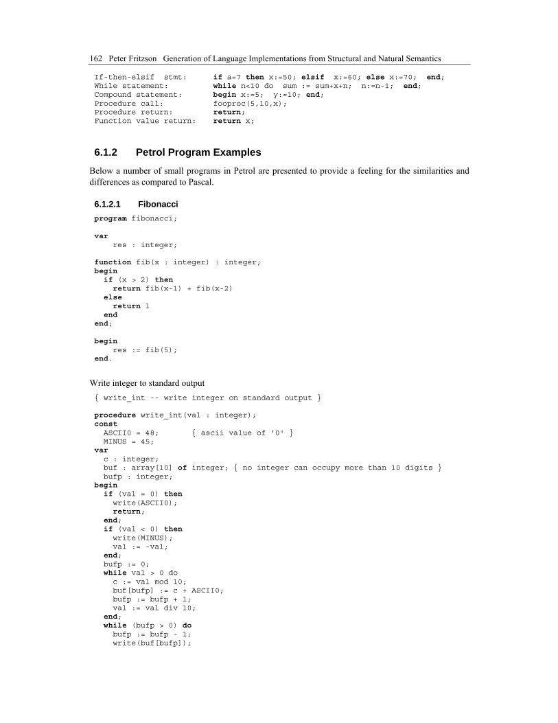
162 Peter Fritzson Generation of Language Implementations from Structural and Natural Semantics
If-then-elsif stmt: if a=7 then x:=50; elsif x:=60; else x:=70; end; While statement: while n<10 do sum := sum+x+n; n:=n-1; end; Compound statement: begin x:=5; y:=10; end; Procedure call: fooproc(5,10,x); Procedure return: return; Function value return: return x;
6.1.2 Petrol Program Examples
Below a number of small programs in Petrol are presented to provide a feeling for the similarities and differences as compared to Pascal.
6.1.2.1 Fibonacci program fibonacci; var res : integer; function fib(x : integer) : integer; begin if (x > 2) then return fib(x-1) + fib(x-2) else return 1 end end; begin res := fib(5); end.
Write integer to standard output { write_int -- write integer on standard output } procedure write_int(val : integer); const ASCII0 = 48; { ascii value of '0' } MINUS = 45; var c : integer; buf : array[10] of integer; { no integer can occupy more than 10 digits } bufp : integer; begin if (val = 0) then write(ASCII0); return; end; if (val < 0) then write(MINUS); val := -val; end; bufp := 0; while val > 0 do c := val mod 10; buf[bufp] := c + ASCII0; bufp := bufp + 1; val := val div 10; end; while (bufp > 0) do bufp := bufp - 1; write(buf[bufp]);

Chapter 6 A Large Translational Semantics 163
end; end;
6.1.2.2 Factorial function fact(n : integer) : integer; var temp : integer; begin if n = 0 then return 1 else temp := fact(n - 1); return n * temp; end; end; begin n := read(); n := n - 48; write_int(fact(n)); write(10); end.
6.1.2.3 Address Test Program program addresstest; var x : integer; p : ^integer; begin x := 65; write(x); p := &x; { take address of x } p^ := 66; write(x); write(10); end.
6.1.2.4 A List Implementation program list_cons; type cons_t = record car : integer; cdr : ^cons_t; end; var list : ^cons_t; function malloc(nbytes : integer) : ^cons_t; extern; function cons(car : integer; cdr : ^cons_t) : ^cons_t; var p : ^cons_t; begin p := malloc(8); p^.car := car; p^.cdr := cdr; return p; end; function car(p : ^cons_t) : integer;

164 Peter Fritzson Generation of Language Implementations from Structural and Natural Semantics
begin return p^.car; end; function cdr(p : ^cons_t) : ^cons_t; begin return p^.cdr; end; begin list := cons(65, cons(10, nil)); write(car(list)); write(car(cdr(list))); end.
6.1.2.5 Arrays and Conditionals program arraytest; const SIZE = 10; var a : array[SIZE] of integer; i : integer; x : real; function foo(i : integer; x : real) : integer; begin { if-then-else } if i < x then i := i + 1; x := x - 1; elsif not(i <> x) then { do nothing } else if i <> 0 then i := -i; else i := 7; end; x := x + 1; write(33); end; return i; end; begin { array indexing } a[1] := 2; a[a[1]-1] := a[1]; { type coercion, integer to real } x := 3; i := trunc(x); x := 4 + 4/2; { calling a function } i := foo(i, x); end.

Chapter 6 A Large Translational Semantics 165
6.2 The Main Module of the Compiler The Petrol language specification in RML consists of approximately 10 modules. The Main module, presented below, ties the generated compiler phases together (see also Figure 6-1).
The parser is generated by Yacc, but called from the generated C version of the main module produced by rml2c. Therefore, only the type signature of parse is present in module Parse below. The linker will link the object files together.
Concerning the main module, the relation main is called when execution start, passing command line arguments. Only the first argument is used as the file name of the Petrol program to be compiled.
The main relation then calls the parser (Parse.parse) through relation parse. If parsing is successful, phase 1 of the static analysis is invoked through the relation static which calls Static.elaborate on the abstract syntax tree of the program.
If static elaboration is successful, the compiler continues by performing flattening of the abstract syntax through relations flatten and Flatten.flatten.
Finally, if flattening is successful, target C code is emitted through a call to emit and FCEmit.emit. The Parse module is presented first. It accepts the name of a file containing the text of a Petrol
program which is parsed and converted to an abstract syntax representation of the same program. Since the parser is implemented by Yacc-generated C code, only the interface part of the Parse module is defined. (* parse.rml *) module Parse: with "absyn.rml" relation parse: string => Absyn.Prog end
The main module of the Petrol specification is presented below. It imports definitions of relations Parse.parse, Static.elaborate, Flatten.flatten and FCEmit.emit from files parse.rml, static.rml, flatten.rml and fcemit.rml respectively. (* main.rml *) module Main: relation main: string list => () end with "parse.rml" with "static.rml" with "flatten.rml" with "fcemit.rml" relation main: string list => () = rule parse(file) ---------------- main(file::_) end relation parse: string => () = rule Parse.parse(file) => ast & static(ast) ---------------- parse(file) rule not Parse.parse(file) => _ & print "Parse.parse failed\n" ---------------- parse(file) => fail end relation static: Absyn.Prog => () = rule Static.elaborate(ast) => tcode & flatten(tcode) ----------------
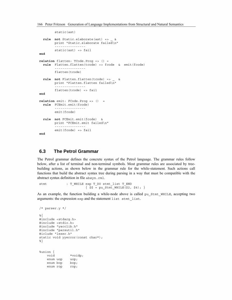
166 Peter Fritzson Generation of Language Implementations from Structural and Natural Semantics
static(ast) rule not Static.elaborate(ast) => _ & print "Static.elaborate failed\n" ---------------- static(ast) => fail end relation flatten: TCode.Prog => () = rule Flatten.flatten(tcode) => fcode & emit(fcode) ---------------- flatten(tcode) rule not Flatten.flatten(tcode) => _ & print "Flatten.flatten failed\n" ---------------- flatten(tcode) => fail end relation emit: FCode.Prog => () = rule FCEmit.emit(fcode) ---------------- emit(fcode) rule not FCEmit.emit(fcode) & print "FCEmit.emit failed\n" ---------------- emit(fcode) => fail end
6.3 The Petrol Grammar The Petrol grammar defines the concrete syntax of the Petrol language. The grammar rules follow below, after a list of terminal and non-terminal symbols. Most grammar rules are associated by tree-building actions, as shown below in the grammar rule for the while-statement. Such actions call functions that build the abstract syntax tree during parsing in a way that must be compatible with the abstract syntax definition in file absyn.rml. stmt : T_WHILE exp T_DO stmt_list T_END { $$ = pu_Stmt_WHILE($2, $4); }
As an example, the function building a while-node above is called pu_Stmt_WHILE, accepting two arguments: the expression exp and the statement list stmt_list. /* parser.y */ %{ #include <stdarg.h> #include <stdio.h> #include "yacclib.h" #include "parsutil.h" #iclude "lexer.h" static void yyerror(const char*); %} %union { void *voidp; enum uop uop; enum bop bop; enum rop rop;

Chapter 6 A Large Translational Semantics 167
enum eop eop; } /* terminals */ %token T_AMPER /* & */ %token T_AND /* and */ %token T_ARRAY /* array */ %token T_ASSIGN /* := */ %token T_BEGIN /* begin */ %token T_CARET /* ^ */ %token T_CAST /* cast */ %token T_COLON /* : */ %token T_COMMA /* , */ %token T_CONST /* const */ %token T_DO /* do */ %token T_DOT /* . */ %token T_ELSE /* else */ %token T_ELSIF /* elseif */ %token T_END /* end */ %token T_EQ /* = */ %token T_EXTERN /* extern */ %token T_FUNCTION /* function */ %token T_GE /* >= */ %token T_GT /* > */ %token <voidp> T_ICON /* <int constant> */ %token <voidp> T_IDENT /* <identifier> */ %token T_IDIV /* div */ %token T_IF /* if */ %token T_IMOD /* mod */ %token T_LBRACK /* [ */ %token T_LE /* <= */ %token T_LPAREN /* ( */ %token T_LT /* < */ %token T_MINUS /* - */ %token T_MUL /* * */ %token T_NE /* <> */ %token T_NOT /* not */ %token T_OF /* of */ %token T_OR /* or */ %token T_PLUS /* + */ %token T_PROCEDURE /* procedure */ %token T_PROGRAM /* program */ %token T_RBRACK /* ] */ %token <voidp> T_RCON /* <real constant>*/ %token T_RDIV /* / */ %token T_RECORD /* record */ %token T_RETURN /* return */ %token T_RPAREN /* ) */ %token T_SEMI /* ; */ %token T_THEN /* then */ %token T_TYPE /* type */ %token T_VAR /* var */ %token T_WHILE /* while */ /* non-terminals */ %type <voidp> block body %type <voidp> const_part const_decls const_decl constant %type <voidp> type_part type_decls type_decl type %type <voidp> var_part var_decls var_decl %type <voidp> sub_part sub_decls sub_decl opt_param_list param_list param %type <voidp> comp_stmt stmt_list stmt elsif_part else_part %type <voidp> opt_exp_list exp_list exp eq_exp rel_exp add_exp %type <voidp> mul_exp unary_exp postfix_exp primary_exp %type <uop> unary_op
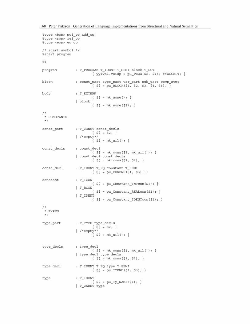
168 Peter Fritzson Generation of Language Implementations from Structural and Natural Semantics
%type <bop> mul_op add_op %type <rop> rel_op %type <eop> eq_op /* start symbol */ %start program %% program : T_PROGRAM T_IDENT T_SEMI block T_DOT { yylval.voidp = pu_PROG($2, $4); YYACCEPT; } block : const_part type_part var_part sub_part comp_stmt { $$ = pu_BLOCK($1, $2, $3, $4, $5); } body : T_EXTERN { $$ = mk_none(); } | block { $$ = mk_some($1); } /* * CONSTANTS */ const_part : T_CONST const_decls { $$ = $2; } | /*empty*/ { $$ = mk_nil(); } const_decls : const_decl { $$ = mk_cons($1, mk_nil()); } | const_decl const_decls { $$ = mk_cons($1, $2); } const_decl : T_IDENT T_EQ constant T_SEMI { $$ = pu_CONBND($1, $3); } constant : T_ICON { $$ = pu_Constant_INTcon($1); } | T_RCON { $$ = pu_Constant_REALcon($1); } | T_IDENT { $$ = pu_Constant_IDENTcon($1); } /* * TYPES */ type_part : T_TYPE type_decls { $$ = $2; } | /*empty*/ { $$ = mk_nil(); } type_decls : type_decl { $$ = mk_cons($1, mk_nil()); } | type_decl type_decls { $$ = mk_cons($1, $2); } type_decl : T_IDENT T_EQ type T_SEMI { $$ = pu_TYBND($1, $3); } type : T_IDENT { $$ = pu_Ty_NAME($1); } | T_CARET type

Chapter 6 A Large Translational Semantics 169
{ $$ = pu_Ty_PTR($2); } | T_ARRAY T_LBRACK constant T_RBRACK T_OF type { $$ = pu_Ty_ARR($3, $6); } | T_RECORD var_decls T_END { $$ = pu_Ty_REC($2); } /* * VARIABLES */ var_part : T_VAR var_decls { $$ = $2; } | /*empty*/ { $$ = mk_nil(); } var_decls : var_decl { $$ = mk_cons($1, mk_nil()); } | var_decl var_decls { $$ = mk_cons($1, $2); } var_decl : T_IDENT T_COLON type T_SEMI { $$ = pu_VARBND($1, $3); } /* * SUB-PROGRAMS */ sub_part : sub_decls | /*empty*/ { $$ = mk_nil(); } sub_decls : sub_decl { $$ = mk_cons($1, mk_nil()); } | sub_decl sub_decls { $$ = mk_cons($1, $2); } sub_decl : T_PROCEDURE T_IDENT opt_param_list T_SEMI body T_SEMI { $$ = pu_SubBnd_PROCBND($2, $3, $5); } | T_FUNCTION T_IDENT opt_param_list T_COLON type T_SEMI body T_SEMI { $$ = pu_SubBnd_FUNCBND($2, $3, $5, $7); } opt_param_list : T_LPAREN param_list T_RPAREN { $$ = $2; } | T_LPAREN T_RPAREN { $$ = mk_nil(); } | /*empty*/ { $$ = mk_nil(); } param_list : param { $$ = mk_cons($1, mk_nil()); } | param T_SEMI param_list { $$ = mk_cons($1, $3); } param : T_IDENT T_COLON type { $$ = pu_VARBND($1, $3); } /* * STATEMENTS */ comp_stmt : T_BEGIN stmt_list T_END { $$ = $2; }

170 Peter Fritzson Generation of Language Implementations from Structural and Natural Semantics
stmt_list : stmt | stmt T_SEMI stmt_list { $$ = pu_Stmt_SEQ($1, $3); } stmt : T_IF exp T_THEN stmt_list elsif_part { $$ = pu_Stmt_IF($2, $4, $5); } | T_WHILE exp T_DO stmt_list T_END { $$ = pu_Stmt_WHILE($2, $4); } | T_IDENT T_LPAREN opt_exp_list T_RPAREN { $$ = pu_Stmt_PCALL($1, $3); } | unary_exp T_ASSIGN exp { $$ = pu_Stmt_ASSIGN($1, $3); } | T_RETURN exp { $$ = pu_Stmt_FRETURN($2); } | T_RETURN { $$ = pu_Stmt_PRETURN(); } | /*empty*/ { $$ = pu_Stmt_SKIP(); } elsif_part : T_ELSIF exp T_THEN stmt_list elsif_part { $$ = pu_Stmt_IF($2, $4, $5); } | else_part else_part : T_ELSE stmt_list T_END { $$ = $2; } | T_END { $$ = pu_Stmt_SKIP(); } /* * EXPRESSIONS */ opt_exp_list : exp_list | /*empty*/ { $$ = mk_nil(); } exp_list : exp { $$ = mk_cons($1, mk_nil()); } | exp T_COMMA exp_list { $$ = mk_cons($1, $3); } exp : eq_exp eq_exp : rel_exp | eq_exp eq_op rel_exp { $$ = pu_Exp_EQUALITY($1, $2, $3); } eq_op : T_EQ { $$ = EOP_EQ; } | T_NE { $$ = EOP_NE; } rel_exp : add_exp | rel_exp rel_op add_exp { $$ = pu_Exp_RELATION($1, $2, $3); } rel_op : T_LT { $$ = ROP_LT; } | T_LE { $$ = ROP_LE; } | T_GE { $$ = ROP_GE; } | T_GT { $$ = ROP_GT; }

Chapter 6 A Large Translational Semantics 171
add_exp : mul_exp | add_exp add_op mul_exp { $$ = pu_Exp_BINARY($1, $2, $3); } add_op : T_OR { $$ = BOP_IOR; } | T_PLUS { $$ = BOP_ADD; } | T_MINUS { $$ = BOP_SUB; } mul_exp : unary_exp | mul_exp mul_op unary_exp { $$ = pu_Exp_BINARY($1, $2, $3); } mul_op : T_AND { $$ = BOP_IAND; } | T_MUL { $$ = BOP_MUL; } | T_RDIV { $$ = BOP_RDIV; } | T_IDIV { $$ = BOP_IDIV; } | T_IMOD { $$ = BOP_IMOD; } unary_exp : postfix_exp | unary_op unary_exp { $$ = pu_Exp_UNARY($1, $2); } unary_op : T_AMPER { $$ = UOP_ADDR; } | T_NOT { $$ = UOP_NOT; } | T_PLUS { $$ = UOP_PLUS; } | T_MINUS { $$ = UOP_MINUS; } postfix_exp : primary_exp | postfix_exp T_CARET { $$ = pu_Exp_UNARY(UOP_INDIR, $1); } | postfix_exp T_DOT T_IDENT { $$ = pu_Exp_FIELD($1, $3); } | postfix_exp T_LBRACK exp T_RBRACK { $$ = pu_Exp_UNARY(UOP_INDIR, pu_Exp_BINARY($1, BOP_ADD, $3)); } | T_IDENT T_LPAREN opt_exp_list T_RPAREN { $$ = pu_Exp_FCALL($1, $3); } | T_CAST T_LPAREN type T_COMMA exp T_RPAREN { $$ = pu_Exp_CAST($3, $5); } primary_exp : T_IDENT { $$ = pu_Exp_IDENT($1); } | T_ICON { $$ = pu_Exp_INT($1); } | T_RCON { $$ = pu_Exp_REAL($1); } | T_LPAREN exp T_RPAREN { $$ = $2; } %%

172 Peter Fritzson Generation of Language Implementations from Structural and Natural Semantics
6.4 Petrol Lexical Syntax The Petrol lexical syntax is described below as regular expressions in Lex syntax. Tokens described by reserved words (and, array, begin, cast, const, do, else, elseif, end, extern, function, div, if, mod, not, of, or, procedure, program, record, return, then, type, var, while) are produced by the function lex_ident, which is not presented here (see appendix **??). Additionally, lex_ident returns the token T_IDENT for identifiers of user-defined variables and procedures. A scanned identifier name is returned through the global variable yyval. (**?? which is a union type of in the Yacc specification, but here only voidp is used here. (but mk_icon, mk_string, mk_char, mk_int)) (pu_ functions in parsutil.c **??)
The function lex_comment reads comment text within curly brackets {} including the final }. These additional functions are found in the file lexutil.c (** see appendix ??). %{ /* lexer.l */ #include "port/config.h" #include "yacclib.h" /* error() */ #include "parsutil.h" #include "parser.h" #include "lexutil.h" ... %} white [ \t\n]+ letter [a-zA-Z_] digit [0-9] ident {letter}({letter}|{digit})* digits {digit}+ icon {digits} pt "." sign [+-] exponent ([eE]{sign}?{digits}) rcon1 {digits}({pt}{digits}?)?{exponent} rcon2 {digits}?{pt}{digits}{exponent}? rcon {rcon1}|{rcon2} %% "{" lex_comment(); {white} ; {ident} return lex_log_token(lex_ident()); {icon} return lex_log_token(lex_icon()); {rcon} return lex_log_token(lex_rcon()); ":=" return lex_log_token(T_ASSIGN); ":" return lex_log_token(T_COLON); "," return lex_log_token(T_COMMA); "." return lex_log_token(T_DOT); "[" return lex_log_token(T_LBRACK); "]" return lex_log_token(T_RBRACK); "(" return lex_log_token(T_LPAREN); ")" return lex_log_token(T_RPAREN); "<>" return lex_log_token(T_NE); "<=" return lex_log_token(T_LE); "<" return lex_log_token(T_LT); "=" return lex_log_token(T_EQ); ">=" return lex_log_token(T_GE); ">" return lex_log_token(T_GT); "-" return lex_log_token(T_MINUS); "*" return lex_log_token(T_MUL); "+" return lex_log_token(T_PLUS); "/" return lex_log_token(T_RDIV);

Chapter 6 A Large Translational Semantics 173
";" return lex_log_token(T_SEMI); "&" return lex_log_token(T_AMPER); "^" return lex_log_token(T_CARET);
6.5 Petrol Abstract Syntax The Petrol abstract syntax in RML form is shown below. There are many similarities compared to the PAM abstract syntax definition in Section 2.6.3, even though the Petrol abstract syntax is more than twice as long. This is mainly due to the presence of declarations and a richer type system that includes arrays, pointers and records as well as functions/procedures. A few additional operators have also been added.
However, some language constructs are not present in the abstract syntax, since they have been eliminated through simple transformations during construction of abstract syntax trees at parse-time. For example, array indexing exp1[exp2] is converted to (exp1+exp2)^ using Petrol’s ability for pointer arithmetic. The following simple transformations are being done at parse time: exp1[exp2] ==> (exp1 + exp2)^ -exp ==> 0 - exp (**?? See function pu_exp_UNARY in parsutil.c ) +exp ==> exp exp1 <> exp2 ==> not(exp1 = exp2) exp1 >= exp2 ==> exp2 <= exp1 exp1 > exp2 ==> exp2 < exp1
In retrospect, having such simplifying transformations at parse-time in the context of a semantic specification for a programming language may not be such a good idea, since it makes the semantic specification less self consistent viewed as a language specification document. In short: if you are looking for the definition of your favorite operator in the semantic specification, you may not find it because it is eliminated at parse time. One the other hand, it can still be argued that the language specification is complete since you will find all operators in the syntactic specification (the grammar), which is part of the complete language specification.
The notion of semantics-oriented abstract syntax is also used for Petrol. Binary arithmetic operators (BinOp) can be arguments to the BINARY constructor, and relational operators (RelOp) can be arguments to the RELATION constructor, except for EQUALITY which belongs to Exp.
Why is EQUALITY a special case that belongs to Exp instead of RELATION? This is because EQUALITY also applies to pointer types, which other relational operators do not allow.
There are also three unary operators (ADDR, INDIR, NOT) which belongs to UnOp and can be arguments to the UNARY constructor.
Identifiers are represented as strings, through the type Ident: type Ident = string
An interesting observation is that there are two sets of constant leaf nodes. One set can be used as right-hand sides in constant declarations, belonging to union type Constant: datatype Constant = INTcon of int (* 55, 36, 999 *) | REALcon of real (* 3.1459, 1.2E-35 *) | IDENTcon of Ident (* foo, fum *)
Another set of nodes can appear in arbitrary expressions and belong to the union type Exp: datatype Exp = INT of int (* 55, 999, *) | REAL of real (* 3.1459, ... *) | IDENT of Ident (* foo, fum ... *)
Why have we chosen to have two sets of constant leaf nodes? We could have used the three leaf nodes belonging to Exp, and thereby made the specification slightly shorter. The current choice of having a special set of Constant nodes is somewhat arbitrary, but the main reason is to make the specification more precise and give the RML system a greater chance to detect type errors in the specification.
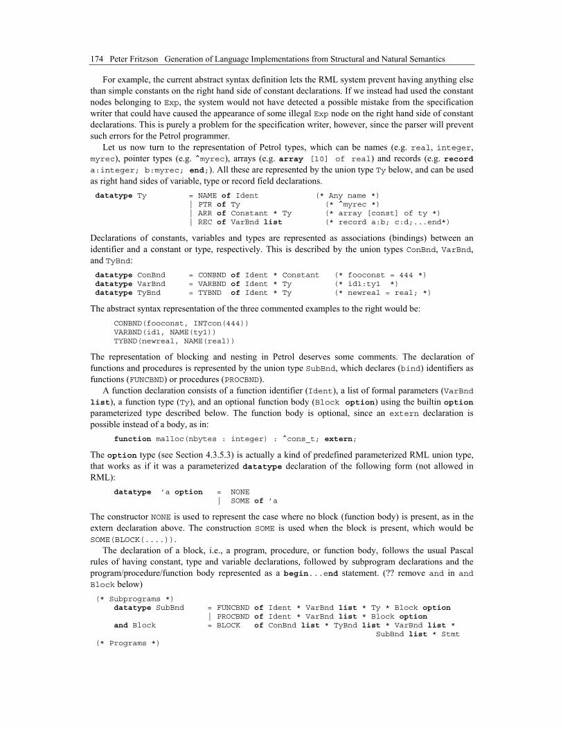
174 Peter Fritzson Generation of Language Implementations from Structural and Natural Semantics
For example, the current abstract syntax definition lets the RML system prevent having anything else than simple constants on the right hand side of constant declarations. If we instead had used the constant nodes belonging to Exp, the system would not have detected a possible mistake from the specification writer that could have caused the appearance of some illegal Exp node on the right hand side of constant declarations. This is purely a problem for the specification writer, however, since the parser will prevent such errors for the Petrol programmer.
Let us now turn to the representation of Petrol types, which can be names (e.g. real, integer, myrec), pointer types (e.g. ^myrec), arrays (e.g. array [10] of real) and records (e.g. record a:integer; b:myrec; end;). All these are represented by the union type Ty below, and can be used as right hand sides of variable, type or record field declarations. datatype Ty = NAME of Ident (* Any name *) | PTR of Ty (* ^myrec *) | ARR of Constant * Ty (* array [const] of ty *) | REC of VarBnd list (* record a:b; c:d;...end*)
Declarations of constants, variables and types are represented as associations (bindings) between an identifier and a constant or type, respectively. This is described by the union types ConBnd, VarBnd, and TyBnd: datatype ConBnd = CONBND of Ident * Constant (* fooconst = 444 *) datatype VarBnd = VARBND of Ident * Ty (* id1:ty1 *) datatype TyBnd = TYBND of Ident * Ty (* newreal = real; *)
The abstract syntax representation of the three commented examples to the right would be: CONBND(fooconst, INTcon(444)) VARBND(id1, NAME(ty1)) TYBND(newreal, NAME(real))
The representation of blocking and nesting in Petrol deserves some comments. The declaration of functions and procedures is represented by the union type SubBnd, which declares (bind) identifiers as functions (FUNCBND) or procedures (PROCBND).
A function declaration consists of a function identifier (Ident), a list of formal parameters (VarBnd list), a function type (Ty), and an optional function body (Block option) using the builtin option parameterized type described below. The function body is optional, since an extern declaration is possible instead of a body, as in: function malloc(nbytes : integer) : ^cons_t; extern;
The option type (see Section 4.3.5.3) is actually a kind of predefined parameterized RML union type, that works as if it was a parameterized datatype declaration of the following form (not allowed in RML): datatype ’a option = NONE | SOME of ’a
The constructor NONE is used to represent the case where no block (function body) is present, as in the extern declaration above. The construction SOME is used when the block is present, which would be SOME(BLOCK(....)).
The declaration of a block, i.e., a program, procedure, or function body, follows the usual Pascal rules of having constant, type and variable declarations, followed by subprogram declarations and the program/procedure/function body represented as a begin...end statement. (?? remove and in and Block below) (* Subprograms *) datatype SubBnd = FUNCBND of Ident * VarBnd list * Ty * Block option | PROCBND of Ident * VarBnd list * Block option and Block = BLOCK of ConBnd list * TyBnd list * VarBnd list * SubBnd list * Stmt (* Programs *)

Chapter 6 A Large Translational Semantics 175
datatype Prog = PROG of Ident * Block
To give an example of abstract syntax, we show the small function car below: function car(p : ^cons_t) : integer; begin return p^.car; end;
This function definition has the following structure represented as abstract syntax, where the begin...end compound statement is eliminated below since it only contains a return statement, but is represented as a statement sequence (SEQ) when it contains two or more statements: FUNCBND(car, VARBND(p, PTR(NAME(cons_t))), NAME(integer), SOME(BLOCK( [], [], [], FRETURN(FIELD(UNARY(INDIR(IDENT(p))), car)) )) )
The complete abstract syntax of Petrol, as specified in module Absyn, is given below. Comments to the right provide examples of concrete syntax of the various constructs. (* absyn.rml *) module Absyn: type Ident = string datatype Constant = INTcon of int (* Ex: 55, 36, 999 *) | REALcon of real (* Ex: 3.1459, 1.2E-35 *) | IDENTcon of Ident (* Ex: foo, fum *) datatype ConBnd = CONBND of Ident * Constant (* fooconst = 444 *) (* Types and variables *) datatype Ty = NAME of Ident (* typename *) | PTR of Ty (* ^typename *) | ARR of Constant * Ty (* array [const] of ty *) | REC of VarBnd list (* record a:b; c:d;... *) and VarBnd = VARBND of Ident * Ty (* id1:ty1 *) datatype TyBnd = TYBND of Ident * Ty (* newreal = real; *) (* Operators *) datatype UnOp = ADDR | INDIR | NOT (* &, ^, not *) datatype BinOp = ADD | SUB | MUL | RDIV | (* +, -, *, /, *) IDIV | IMOD | IAND | IOR (* div, mod, and, or *) datatype RelOp = LT | LE (* <, <= *) (* Expression nodes *) datatype Exp = INT of int (* 55, 999, *) | REAL of real (* 3.1459, ... *) | IDENT of Ident (* foo, fum ... *) | CAST of Ty * Exp (* real(3+5) *) | FIELD of Exp * Ident (* recexp.fieldid *) | UNARY of UnOp * Exp (* unop expr *) | BINARY of Exp * BinOp * Exp (* e1 binop e2 *) | RELATION of Exp * RelOp * Exp (* e1 relop e2 *) | EQUALITY of Exp * Exp (* e1 = e2 *) | FCALL of Ident * Exp list (* foo(e1,e2,...) *) (* Statements *) datatype Stmt = ASSIGN of Exp * Exp (* x := 1+y; *)

176 Peter Fritzson Generation of Language Implementations from Structural and Natural Semantics
| PCALL of Ident * Exp list (* f2(a1,a2+5,a3,...) *) | FRETURN of Exp (* return e1+5 *) | PRETURN (* return *) | WHILE of Exp * Stmt (* while e1 do s1 end *) | IF of Exp * Stmt * Stmt (* if e1 then s1 else s2*) | SEQ of Stmt * Stmt (* s1; s2 *) | SKIP (* empty statement *) (* Subprograms *) (* Block option is needed for Petrol extern declarations without body *) datatype SubBnd = FUNCBND of Ident * VarBnd list * Ty * Block option | PROCBND of Ident * VarBnd list * Block option and Block = BLOCK of ConBnd list * TyBnd list * VarBnd list * SubBnd list * Stmt (* Programs *) datatype Prog = PROG of Ident * Block end (* of interface section of Absyn *) (**?? Where do we find a CHAR node for inline string constants? CHAR is a predefined type in Petrol, just like INT or REAL. character constants are not supported by Petrol: ’a’ - or would be converted to int. ??NOTE: Petrol has no strings - just like in Diesel *)
6.6 TCode Representation The main part of Petrol static semantics (defined by the modules Static and Types) performs type checking and conversion of Petrol abstract syntax to the TCode (Tree Code) representation. Thus, it is appropriate to define TCode (described in module TCode) before going into the details of translation. As we shall see, this representation is still rather high level and rather close to the abstract syntax representation of Petrol as defined in module Absyn.
When importing definitions from Absyn or TCode, it is necessary to use the module prefix which solves the problem of possible collisions between node constructor names, which would otherwise be the case e.g. between Absyn.ADDR and TCode.ADDR. If a constructor occurs without a module prefix, it is always defined in the same module where it is referenced.
The full TCode definition follows below. Headers and comments have been inserted to increase readability.
6.6.1 TCode Module Header (* tcode.rml *) module TCode:
6.6.2 Types
Declaration nodes are absent from TCode. All type names have been eliminated and replaced by a direct representation of corresponding types. Types are represented by type nodes which are largely similar to the abstract syntax versions. Inline CHAR constants do not exist in Petrol, but you may declare variables which have the type CHAR, array of characters, etc.
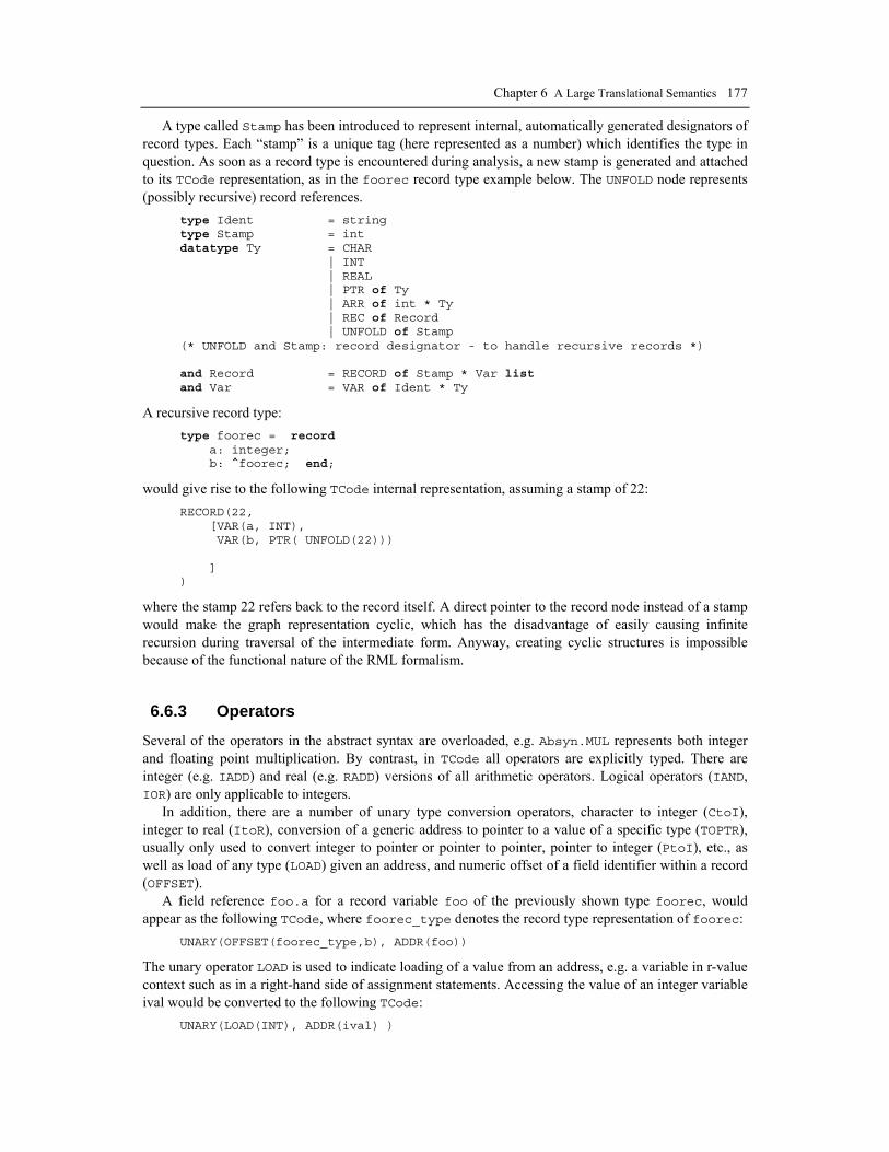
Chapter 6 A Large Translational Semantics 177
A type called Stamp has been introduced to represent internal, automatically generated designators of record types. Each “stamp” is a unique tag (here represented as a number) which identifies the type in question. As soon as a record type is encountered during analysis, a new stamp is generated and attached to its TCode representation, as in the foorec record type example below. The UNFOLD node represents (possibly recursive) record references. type Ident = string type Stamp = int datatype Ty = CHAR | INT | REAL | PTR of Ty | ARR of int * Ty | REC of Record | UNFOLD of Stamp (* UNFOLD and Stamp: record designator - to handle recursive records *) and Record = RECORD of Stamp * Var list and Var = VAR of Ident * Ty
A recursive record type: type foorec = record a: integer; b: ^foorec; end;
would give rise to the following TCode internal representation, assuming a stamp of 22: RECORD(22, [VAR(a, INT), VAR(b, PTR( UNFOLD(22))) ] )
where the stamp 22 refers back to the record itself. A direct pointer to the record node instead of a stamp would make the graph representation cyclic, which has the disadvantage of easily causing infinite recursion during traversal of the intermediate form. Anyway, creating cyclic structures is impossible because of the functional nature of the RML formalism.
6.6.3 Operators
Several of the operators in the abstract syntax are overloaded, e.g. Absyn.MUL represents both integer and floating point multiplication. By contrast, in TCode all operators are explicitly typed. There are integer (e.g. IADD) and real (e.g. RADD) versions of all arithmetic operators. Logical operators (IAND, IOR) are only applicable to integers.
In addition, there are a number of unary type conversion operators, character to integer (CtoI), integer to real (ItoR), conversion of a generic address to pointer to a value of a specific type (TOPTR), usually only used to convert integer to pointer or pointer to pointer, pointer to integer (PtoI), etc., as well as load of any type (LOAD) given an address, and numeric offset of a field identifier within a record (OFFSET).
A field reference foo.a for a record variable foo of the previously shown type foorec, would appear as the following TCode, where foorec_type denotes the record type representation of foorec: UNARY(OFFSET(foorec_type,b), ADDR(foo))
The unary operator LOAD is used to indicate loading of a value from an address, e.g. a variable in r-value context such as in a right-hand side of assignment statements. Accessing the value of an integer variable ival would be converted to the following TCode: UNARY(LOAD(INT), ADDR(ival) )

178 Peter Fritzson Generation of Language Implementations from Structural and Natural Semantics
The unary operator TOPTR is a pointer conversion which conveys information about which type of value a pointer is pointing to. This is used primarily for address arithmetic needed when accessing or storing into array elements. Both LOAD and TOPTR are type specific, i.e., they only appear parameterized by type, e.g. LOAD(INT), or TOPTR(REAL).
This is natural, since the address computation needed e.g. for array indexing is dependent on the size of the type of elements to be indexed, e.g. 8 bytes per element for real double precision and 4 bytes for 32-bit integers. Remember that already at parse time, array indexing exp1[exp2] operations were converted to (exp1+exp2)^ using Petrol’s ability for pointer arithmetic. Thus, TOPTR is a special type conversion operator that is only applied to addresses and pointers to provide additional pointer type information, for example the size of pointed to data elements, needed for correct address arithmetic in pointer expressions created through array indexing.
For example, an array indexing operation Xarr[ind] of a real array in r-value context, that was already converted to pointer arithmetic (Xarr+ind)^ when the abstract syntax tree was built, would appear as follows converted to TCode: UNARY(LOAD(REAL), BINARY(UNARY(TOPTR(REAL), ADDR(Xarr)), PADD(REAL), UNARY(LOAD(INT),ADDR(Ind)) ) ).
Note that TOPTR will cast anything to a pointer. CtoI, ItoR, PtoI and ItoC are used for type conversions e.g. in parameter passing or conversions in assignment statements. ItoR performs an actual conversion of the integer to a real value.
There are also a number of operators for pointer arithmetic and pointer comparisons (PADD, PSUB, PDIFF, PLT, PLE, and PEQ). All of these have a type argument since they are used in arbitrary pointer expressions. Such pointer expressions can be created from array indexing expressions, where the array element type of course can be any type. (* A number of unary conversion operators, augmented with LOAD and OFFSET *) datatype UnOp = CtoI | ItoR | RtoI | ItoC | TOPTR of Ty | PtoI | LOAD of Ty | OFFSET of Record * Ident (* Typed binary operators *) datatype BinOp = IADD | ISUB | IMUL | IDIV | IMOD | IAND | IOR | ILT | ILE | IEQ | RADD | RSUB | RMUL | RDIV | RLT | RLE | REQ (* Pointer operators with type parameter *) | PADD of Ty | PSUB of Ty | PDIFF of Ty | PLT of Ty | PLE of Ty | PEQ of Ty
6.6.4 Expressions
Expressions contain constants, unary and binary operator applications, function calls, and address- of operators (ADDR). Such ADDR operators have been inserted for all identifiers representing simple variables. Thus an integer variable reference IDENT(x) in abstract syntax (r-value context) will be converted to UNARY(LOAD(INT),ADDR(x)) in TCode. datatype Exp = ICON of int | RCON of real | ADDR of Ident | UNARY of UnOp * Exp | BINARY of Exp * BinOp * Exp | FCALL of Ident * Exp list
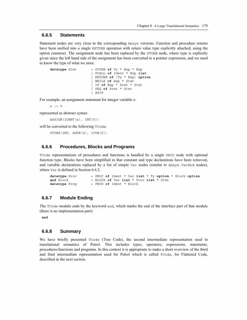
Chapter 6 A Large Translational Semantics 179
6.6.5 Statements
Statement nodes are very close to the corresponding Absyn versions. Function and procedure returns have been unified into a single RETURN operation with return value type explicitly attached, using the option construct. The assignment node has been replaced by the STORE node, where type is explicitly given since the left hand side of the assignment has been converted to a pointer expression, and we need to know the type of what we store. datatype Stmt = STORE of Ty * Exp * Exp | PCALL of Ident * Exp list | RETURN of (Ty * Exp) option | WHILE of Exp * Stmt | IF of Exp * Stmt * Stmt | SEQ of Stmt * Stmt | SKIP
For example, an assignment statement for integer variable x: x := 5
represented as abstract syntax: ASSIGN(IDENT(x), INT(5))
will be converted to the following TCode: STORE(INT, ADDR(x), ICON(5))
6.6.6 Procedures, Blocks and Programs
TCode representations of procedures and functions is handled by a single PROC node with optional function type. Blocks have been simplified in that constant and type declarations have been removed, and variable declarations replaced by a list of simple Var nodes (similar to Absyn.VarBnd nodes), where Var is defined in Section 6.6.2. datatype Proc = PROC of Ident * Var list * Ty option * Block option and Block = BLOCK of Var list * Proc list * Stmt datatype Prog = PROG of Ident * Block
6.6.7 Module Ending
The TCode module ends by the keyword end, which marks the end of the interface part of that module (there is no implementation part): end
6.6.8 Summary
We have briefly presented TCode (Tree Code), the second intermediate representation used in translational semantics of Petrol. This includes types, operators, expressions, statements, procedures/functions and programs. In this context it is appropriate to make a short overview of the third and final intermediate representation used for Petrol which is called FCode, for Flattened Code, described in the next section.

180 Peter Fritzson Generation of Language Implementations from Structural and Natural Semantics
6.7 FCode – Flattened Code representation FCode is almost identical to TCode. The only difference between the two representations is the introduction of the DISPLAY node, changes in the BLOCK, PROC, and PROG nodes, and the removal of the ADDR node.
Nesting of scopes have been removed and flattened to a single scope in FCode. Thus, a BLOCK in FCode may not contain other procedure or function blocks. All procedure/function blocks (represented as PROC nodes that contain BLOCKs) have been placed in a single PROC list in the program node. The nesting level is instead indicated by the Level attribute of BLOCK.
A reference to a variable (local or non-local) is converted to a reference of a corresponding field of an activation record via a DISPLAY node. This can later be implemented by a small array (a display) of pointers to activation records, indexed by scope level, or alternatively as indirections through a chain of pointers called static links. The only identifiers left in the FCode intermediate form are field names and procedure/function names. (* fcode.rml *) module FCode: type Level = int type Ident = string type Stamp = int datatype Ty = CHAR | INT | REAL | PTR of Ty | ARR of int * Ty | REC of Record | UNFOLD of Stamp and Record = RECORD of Stamp * Var list and Var = VAR of Ident * Ty datatype UnOp = CtoI | ItoR | RtoI | ItoC | TOPTR of Ty | PtoI | LOAD of Ty | OFFSET of Record * Ident datatype BinOp = IADD | ISUB | IMUL | IDIV | IMOD | IAND | IOR | ILT | ILE | IEQ | RADD | RSUB | RMUL | RDIV | RLT | RLE | REQ | PADD of Ty | PSUB of Ty | PDIFF of Ty | PLT of Ty | PLE of Ty | PEQ of Ty datatype Exp = ICON of int | RCON of real | DISPLAY of Level | UNARY of UnOp * Exp | BINARY of Exp * BinOp * Exp | FCALL of Ident * Exp list datatype Stmt = STORE of Ty * Exp * Exp | PCALL of Ident * Exp list | RETURN of (Ty * Exp) option | WHILE of Exp * Stmt | IF of Exp * Stmt * Stmt | SEQ of Stmt * Stmt | SKIP (* Block has a scope Level. When referencing a variable (local or non-local) * go through a DISPLAY. The only identifiers left are field names and procedure * names *) datatype Block = BLOCK of Level * Record * Stmt datatype Proc = PROC of Ident * Var list * Ty option * Block option

Chapter 6 A Large Translational Semantics 181
datatype Prog = PROG of Proc list * Ident end
This concludes the short overview of the FCode intermediate representation. Next we will present auxiliary structures such as environments and additional type representations which are needed to specify the translation of Petrol.
6.8 Environment Representation In addition to the intermediate program representations Absyn, TCode, and FCode, some structures are needed to represent environments, (sometimes known as symbol tables), that contain bindings of all entities declared in Petrol programs to be translated by the generated compiler. Such entities include variables, types, constants and procedures/functions that may be referenced during semantic analysis.
The static environment (TCode.Env) is currently used only during translation from abstract syntax to TCode and discarded afterwards. However, it could be saved if we need this symbol information in a debugger or an incremental compilation system. By contrast, the dynamic environment is created at run-time by the executing code, and represented as a stack of activation records. To further complicate the picture, another static environment (FCode.Env, see Section 6.12.1) is created by module FCode, since this is needed during the process of flattening nested scopes. This environment is however very simple in structure since it only contains small procedure descriptors to indicate scope level.
A binding is a pair (identifier, bound-value), where the possible bound descriptors are defined by the datatype Bnd. For example, the bound value for a function includes a list of parameter types and the function type. A bound constant definition associates a constant value (a Con node, INTcon, or REALcon) as the bound value. (* Datatypes for the static environment, defined in module Static. *) datatype Con = INTcon of int | REALcon of real datatype Bnd = VARbnd of Types.Ty | CONSTbnd of Con | FUNCbnd of Types.Ty list * Types.Ty | PROCbnd of Types.Ty list | TYPEbnd of Types.Ty | NILbnd type Binding = TCode.Ident * Bnd type Env = Binding list
The initial system environment is shown below. It includes type bindings for the standard Petrol types integer, real, and char; the standard functions read, write, and trunc; and the null pointer nil. val env_init = [ ("integer", TYPEbnd(Types.ARITH(Types.INT)) ) , ("real", TYPEbnd(Types.ARITH(Types.REAL)) ) , ("char", TYPEbnd(Types.ARITH(Types.CHAR)) ) , ("read", FUNCbnd([], Types.ARITH(Types.INT)) ) , ("write", PROCbnd[Types.ARITH(Types.INT]) , ("trunc", FUNCbnd([Types.ARITH(Types.REAL)],Types.ARITH(Types.INT))) , ("nil", NILbnd ) ]
At any given point in time during the translation, the environment can be represented as a linear list of bindings. When entering a scope, e.g. of a procedure, the bindings from that scope are added (pushed on the environment stack) at the front of this linear list. When exiting a scope, all declarations from that scope are popped from the environment.

182 Peter Fritzson Generation of Language Implementations from Structural and Natural Semantics
Figure 6-2 shows the appearance of the environment after entering the function fib below. The outermost scope level contains the pre-defined procedures, types, and constants. The program creates a new scope level which contains the variable res and the function fib. The scope of the function fib itself only introduces the integer formal parameter x. program fibonacci; var res : integer; function fib(x : integer) : integer; ... end
integer: TYPEbnd(INT) real: TYPEbnd(REAL) char: TYPEbnd(CHAR) read: FUNCbnd([],INT)write: PROCbnd([INT])trunc: FUNCbnd([INT],INT)nil: NILbnd
res: VARbnd(INT) fib: FUNCbnd([INT],INT)
x: VARbnd(INT)
Scope level -1
Scope level 0
Scope level 1
Figure 6-2. The environment, represented as a stack that grows downwards, after entering the scope level of function fib.
For translational semantic descriptions of languages which are more complex than Petrol, e.g. the RML language itself, the environment may be represented as a recursive structure of whole subenvironments.
An environment representation as a linear list is simple and provides a declarative environment definition, but will give rather inefficient lookup when many bindings have been stored. As an alternative, an external RML module that represents environments as balanced binary trees is available for use when high efficiency is needed. The simple lookup relation for linear search of the environment list is shown below. relation lookup: (Env, Ident) => Bnd =
rule key1 = key0 ---------------- lookup((key1,bnd)::_, key0) => bnd rule not key1 = key0 & lookup(env, key0) => bnd ---------------- lookup((key1,_)::env, key0) => bnd
end (* lookup *)
The simplicity of the linear list environment representation makes it useful when prototyping language specifications. An abstract interface to a separate environment module is however desirable to eliminate dependencies on the specific choice of data structures to represent the environment. Using such an abstract interface would also slightly change the appearance of some semantic rules which implicitly assume a list representation for pattern matching on environment structures.
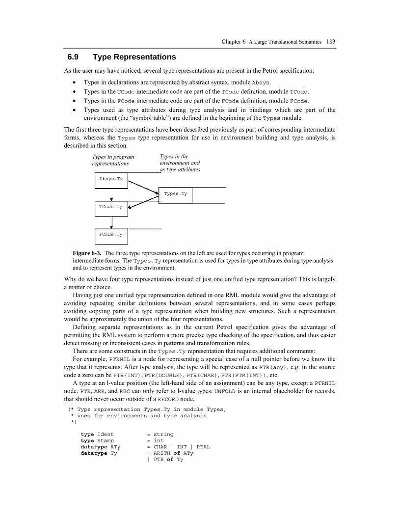
Chapter 6 A Large Translational Semantics 183
6.9 Type Representations As the user may have noticed, several type representations are present in the Petrol specification:
• Types in declarations are represented by abstract syntax, module Absyn. • Types in the TCode intermediate code are part of the TCode definition, module TCode. • Types in the FCode intermediate code are part of the FCode definition, module FCode. • Types used as type attributes during type analysis and in bindings which are part of the
environment (the “symbol table”) are defined in the beginning of the Types module.
The first three type representations have been described previously as part of corresponding intermediate forms, whereas the Types type representation for use in environment building and type analysis, is described in this section.
Absyn.Ty
TCode.Ty
Types.Ty
FCode.Ty
Types in program representations
Types in theenvironment andas type attributes
Figure 6-3. The three type representations on the left are used for types occurring in program intermediate forms. The Types.Ty representation is used for types in type attributes during type analysis and to represent types in the environment.
Why do we have four type representations instead of just one unified type representation? This is largely a matter of choice.
Having just one unified type representation defined in one RML module would give the advantage of avoiding repeating similar definitions between several representations, and in some cases perhaps avoiding copying parts of a type representation when building new structures. Such a representation would be approximately the union of the four representations.
Defining separate representations as in the current Petrol specification gives the advantage of permitting the RML system to perform a more precise type checking of the specification, and thus easier detect missing or inconsistent cases in patterns and transformation rules.
There are some constructs in the Types.Ty representation that requires additional comments: For example, PTRNIL is a node for representing a special case of a null pointer before we know the
type that it represents. After type analysis, the type will be represented as PTR(any), e.g. in the source code a zero can be PTR(INT), PTR(DOUBLE), PTR(CHAR), PTR(PTR(INT)), etc.
A type at an l-value position (the left-hand side of an assignment) can be any type, except a PTRNIL node. PTR, ARR, and REC can only refer to l-value types. UNFOLD is an internal placeholder for records, that should never occur outside of a RECORD node. (* Type representation Types.Ty in module Types, * used for environments and type analysis *) type Ident = string type Stamp = int datatype ATy = CHAR | INT | REAL datatype Ty = ARITH of ATy | PTR of Ty
184 Peter Fritzson Generation of Language Implementations from Structural and Natural Semantics
| PTRNIL | ARR of int * Ty | REC of Record | UNFOLD of Stamp and Record = RECORD of Stamp * (Ident * Ty) list
6.9.1 Type Module Operations
The following is the list of signatures of exported relations of the Types module, as specified in its interface section. (* inspect a record by unfolding it one level *) relation unfold_rec: Types.Record => (Types.Ident * Types.Ty) list (* convert Types types to TCode types *) relation ty_cnv: Types.Ty => TCode.Ty relation rec_cnv: Types.Record => TCode.Record (* apply usual rvalue decay to exp:ty *) relation decay: (TCode.Exp, Types.Ty) => (TCode.Exp, Types.Ty) (* apply the assignment conversions to an rvalue *) relation asg_cnv: (TCode.Exp, Types.Ty, Types.Ty) => TCode.Exp (* apply the cast conversions to a decayed rvalue *) relation cast_cnv: (TCode.Exp, Types.Ty, Types.Ty) => TCode.Exp (* apply the conditional conversions to a decayed rvalue *) relation cond_cnv: (TCode.Exp, Types.Ty) => TCode.Exp (* make an equality expression out of two decayed rvalues *) relation eq_cnv: (TCode.Exp, Types.Ty, TCode.Exp, Types.Ty) => TCode.Exp (* make a relation expression out of two decayed rvalues *) relation rel_cnv: (TCode.Exp, Types.Ty, Absyn.RelOp, TCode.Exp, Types.Ty) => TCode.Exp (* make a binary arithmetic expression out of two decayed rvalues *) relation bin_cnv: (TCode.Exp, Types.Ty, Absyn.BinOp, TCode.Exp, Types.Ty) => (TCode.Exp,Types.Ty) end
6.10 The Static Module The Static module, together with the Types module, describe the main part of the translation of Petrol constructs to TCode. This translation process is called elaboration. There are elaboration relations for most Petrol constructs. The relation elab_stmt translates statements, the relations elab_rvalue and elab_lvalue translate right-hand side and left-hand side expressions, respectively; elab_const elaborates constant declarations and elab_ty translates type representations, elab_subbnds translates procedure and function declarations, etc.
6.10.1 Overview
In this section we present an overview of the translation process for various Petrol constructs. Detailed comments follow later, together with the relations. The topmost relation in module Static is elaborate, which translates a whole program to TCode:

Chapter 6 A Large Translational Semantics 185
relation elaborate: Absyn.Prog => TCode.Prog = (* Elaborate a program *)
rule elab_block(NONE, env_init, block) => block' ---------------- elaborate(Absyn.PROG(id,block)) => TCode.PROG(id,block') end
6.10.1.1 Block Translation
The relation elab_block elaborates a whole block. It accepts an optional function type (only used for function blocks to check return statements), the current (initial) environment, and a BLOCK node, which at the uppermost level is a program block, but could also be a function or procedure block.
Constants, types, variables and subprograms are elaborated in the usual order. The relations elab_consts and elab_vars directly push constant and type bindings on the current environment.
The elaboration of variable declarations is performed in a few small steps. First, elab_vars converts a sequence of abstract syntax VARBND(id,ty) nodes to a linear sequence pre_vars of pairs (identifier, type) where type is using module Types intermediate type representation, and type aliases have been removed (e.g. in type ti=integer; var x:ti; substituting type alias ti, obtaining var x:integer;). Then mkvar is applied to each pair, (by map), producing a new list of TCode.VAR(id,ty’) nodes, where ty’ uses the TCode type representation since it is now part of the TCode intermediate program representation. Finally, mkvarbnd is applied to these nodes producing a list of pairs (id,VARbnd(ty’)) (see Section 6.8) which is pushed on, i.e., appended at the front of, the current environment.
Then subprograms, i.e., procedures or functions declared in the current block, are elaborated. Finally, the body of the current block, a begin...end statement, is elaborated by elab_stmt. The optional function type fty is passed to elab_stmt in case a return statement needs to be checked for a function block.
The end result is a TCode.BLOCK(vars',subbnds',stmt') node, which contains TCode representations of variables, subprograms and the block statement, thus eliminating all constant and type declarations. This will later be passed on (see Section 6.2) to relation Flatten.flatten for flattening, and further to FCEmit.emit for final code generation. relation elab_block: (Types.Ty option, Env, Absyn.Block) => TCode.Block = (* Elaborate a whole block *) rule elab_consts(env0, consts) => env1 & (* also pushes on env *) elab_types(env1, types) => env2 & (* also pushes on env * elab_vars(env2, vars, []) => pre_vars & (* only makes pre_vars alst *) map(mkvar, pre_vars) => vars' & map(mkvarbnd, pre_vars) => varenv & list_append(varenv, env2) => env3 & (* Now, push vars on env *) elab_subbnds(env3, subbnds, []) => (env4,subbnds') & elab_stmt(fty, env4, stmt) => stmt' ---------------- elab_block(fty, env0, Absyn.BLOCK(consts,types,vars,subbnds,stmt)) => TCode.BLOCK(vars', subbnds', stmt') end
6.10.1.2 A Translated Example
As an example, regard the contrived function addpi: function addpi(y: real) : real; const pi = 3.14159; type dreal = real; var x: dreal; begin x := pi+y; return x;
186 Peter Fritzson Generation of Language Implementations from Structural and Natural Semantics
end;
which has the following structure in abstract syntax: FUNCBND(addpi, [VARBND(y, NAME(real))], NAME(real), SOME(BLOCK( [CONBND(pi,REALcon(3.14159))], [TYBND(dreal,NAME(real))], [VARBND(x,NAME(dreal))], [], SEQ( ASSIGN(IDENT(x), BINARY(IDENT(pi), ADD, IDENT(y)), FRETURN(IDENT(x)) ) )) )
and is translated to a binding and TCode intermediate code. The binding (addpi,FUNCbnd([REAL],REAL)) is pushed on the environment. The intermediate code is represented as a TCode PROC node that includes a TCode BLOCK node: PROC(addpi, [VAR(y,REAL)], SOME(REAL), SOME(BLOCK( [VAR(y,REAL)], [], SEQ( STORE(REAL, ADDR(x), BINARY(RCON(3.14159), RADD, UNARY(LOAD,ADDR(y)))), RETURN(SOME(REAL,UNARY(LOAD,ADDR(x))) ) ) )) )
6.10.1.3 Functions and procedures
Translation of functions or procedures is different from translating main programs in that formal parameters and possible return types must be handled. This translation is accomplished by relation elab_subbnd, which produces a TCode representation of the procedure or function, and an updated environment. We focus on the first rule, describing the translation of a function binding, since the rule for procedures is just a similar, but simplified, version of the first rule.
The function type (ty) is elaborated and expanded into the intermediate type representation (ty0), which is decayed (simplified) into more primitive types (ty1, e.g. including conversion of array types to pointer types), and then converted to TCode type representation (ty2).
The formal parameter list is elaborated into a triple of (formals’, argenv, argtys), where formals’ is a list of VAR nodes, suitable for inclusion in a PROC; argenv is an “argument” environment, i.e., a list of VARbnd nodes suitable for pushing on the environment; and argtys is a list of formal argument types suitable as part of the FUNCbnd node to be pushed on the environment.
Then the function binding is pushed on the environment producing env1, followed by the formal parameter bindings, producing env2.
Finally, elab_body is called, which in turn calls elab_block to elaborate the function block.The end result of the elaboration is an updated environment and a TCode.PROC node. relation elab_subbnd: (Env, Absyn.SubBnd) => (Env, TCode.Proc) = (* Elaborate function or procedure bindings. * translate a whole function or procedure to Tcode, * and an updated environment, where the new proc/func has been inserted *)
Chapter 6 A Large Translational Semantics 187
(* elaborate a function *) rule elab_ty(env0, ty) => ty0 & decay_formal_ty(ty0) => ty1 & (* ret ARR ==> ret PTR *) Types.ty_cnv(ty1) => ty2 & elab_formals(env0, formals) => (formals’, argenv, argtys) & let env1 = (id, FUNCbnd(argtys,ty1))::env0 & list_append(argenv, env1) => env2 & elab_body(SOME(ty1), env2, block) => block’ ---------------- elab_subbnd(env0, Absyn.FUNCBND(id,formals,ty,block)) => (env1, TCode.PROC(id,formals’,SOME(ty2),block’)) (* elaborate a procedure *) rule elab_formals(env0, formals) => (formals’, argenv, argtys) & let env1 = (id, PROCbnd(argtys))::env0 & list_append(argenv, env1) => env2 & elab_body(NONE, env2, block) => block’ ---------------- elab_subbnd(env0, Absyn.PROCBND(id,formals,block)) => (env1, TCode.PROC(id,formals’,NONE,block’)) end relation elab_body: (Types.Ty option, Env, Absyn.Block option) => TCode.Block option = (* Elaborate procedure/function body. (fty is optional function type) * Extern declarations are also handled, with empty body represented as NONE. *) axiom elab_body(_, _, NONE) => NONE rule elab_block(fty, env, block) => block’ ---------------- elab_body(fty, env, SOME(block)) => SOME(block’) end
6.10.1.4 Statements
The relation for statement translation is elab_stmt(tyopt,env,stmt) => stmt’, which can handle all abstract syntax statement node types: Absyn.ASSIGN, Absyn.PCALL, Absyn.FRETURN, Absyn.PRETURN, Absyn.WHILE, Absyn.IF, Absyn.SEQ and Absyn.SKIP.
6.10.1.5 Expressions
The primary relation for translating expressions is the elab_rvalue relation, which translates all expressions that occur in r-value context (value context) into pairs of type (Types.ty, TCode.Exp). The type is kept around for type checking and type inference as well as insertion of type conversions.
The only exception are l-value expressions which for example occur in the left hand side of assignment statements, or as actual arguments to reference parameters for programming languages that include such features. Translation of l-value expression is handled by the relation elab_lvalue.
A number of additional functions are called by eval_rvalue, and a few also by elab_lvalue. For example, to translate identifiers, elab_rvalue calls rvalue_id. For identifiers which are
constants, TCON.ICON and TCON.RCON nodes are produced, respectively. For variables, rvalue_id inserts a TCode.ADDR node and calls rvalue_var to also insert a TCode.UNARY(TCode.LOAD(ty),...) node via mkload. Thus, an Absyn.IDENT(x) node of a real variable x will become TCode.UNARY(TCode.LOAD(REAL), ADDR(x)).

188 Peter Fritzson Generation of Language Implementations from Structural and Natural Semantics
6.10.1.6 Assignment Conversion
An important topic is a variant of type conversion called assignment conversion. For example, assignment type conversion needs to be done when assigning an integer value to a real-typed variable, as in the example below: rval := 55;
where the integer value 55 need to be converted to a real constant 55.0 before being assigned to the real-typed variable rval. Sometimes a constant expression can be converted and evaluated at compile time, but usually a conversion operation need to be inserted, to eventually give rise to the appropriate conversion code. Assignment conversion also occurs when passing actual arguments to formal parameters at function/procedure calls, since in a sense the actual argument is “assigned to” the formal parameter.
Code for performing assignment conversion is produced by the relation Types.asg_cnv(exp,ty’,ty), which is called by elab_args to perform assignment conversion of a list of actual arguments and by elab_stmt to perform assignment conversion for the assignment statement.
6.10.1.7 Constants and Types
As already remarked, constant and type declarations will disappear after elaboration. They will not be present in the TCode, but instead will cause constant (CONSTbnd) and type (TYPEbnd) bindings to be inserted into the environment. References to constant and type names in the right-hand sides of such declarations will be expanded. The topmost function for constant declaration elaboration is elab_consts, and for type declarations elab_types.
6.10.1.8 Decay of Types and Expressions
Decay is performed when elaborating certain program constructs, and was already mentioned in the context of function types. But what is decay? What is a decayed r-value? Decay is essentially a process of type simplification and expression conversion, where program types are decayed into simpler, more machine-oriented types and expressions converted accordingly. For example, a character is represented as (i.e., it decays to) a machine integer, an array reference will decay to a pointer indirection, etc. These conversion rules are identical to those of the C language:
• char to int • float to double • array of Tptr to T
Thus, a decayed r-value is a right-hand side expression within which this type simplification has been performed. See relation Types.decay in Section 6.11.4.
Another advantage of performing type decay is that it simplifies the type lattice, so that for example types like char and float need not be considered any longer.
6.10.2 Module Header
The complete Static module follows now, interspersed by appropriate headers and comments. We first show the module header. (* static.rml *) module Static: with "absyn.rml" with "tcode.rml" relation elaborate: Absyn.Prog => TCode.Prog end
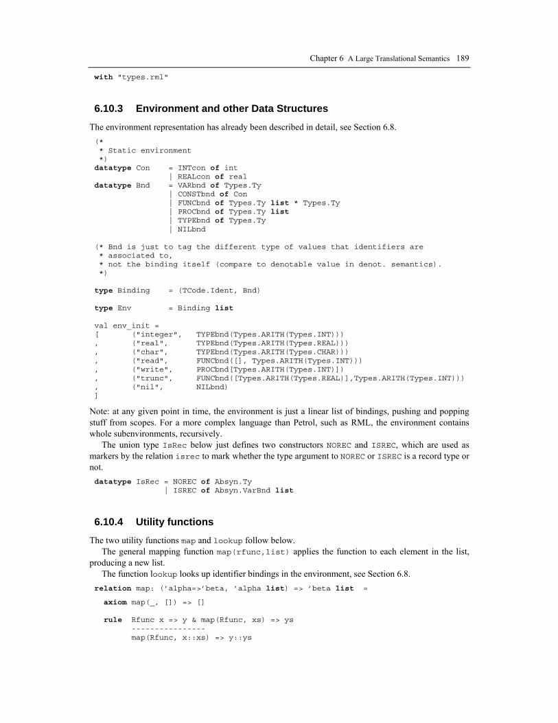
Chapter 6 A Large Translational Semantics 189
with "types.rml"
6.10.3 Environment and other Data Structures
The environment representation has already been described in detail, see Section 6.8. (* * Static environment *) datatype Con = INTcon of int | REALcon of real datatype Bnd = VARbnd of Types.Ty | CONSTbnd of Con | FUNCbnd of Types.Ty list * Types.Ty | PROCbnd of Types.Ty list | TYPEbnd of Types.Ty | NILbnd (* Bnd is just to tag the different type of values that identifiers are * associated to, * not the binding itself (compare to denotable value in denot. semantics). *) type Binding = (TCode.Ident, Bnd) type Env = Binding list val env_init = [ ("integer", TYPEbnd(Types.ARITH(Types.INT))) , ("real", TYPEbnd(Types.ARITH(Types.REAL))) , ("char", TYPEbnd(Types.ARITH(Types.CHAR))) , ("read", FUNCbnd([], Types.ARITH(Types.INT))) , ("write", PROCbnd[Types.ARITH(Types.INT)]) , ("trunc", FUNCbnd([Types.ARITH(Types.REAL)],Types.ARITH(Types.INT))) , ("nil", NILbnd) ]
Note: at any given point in time, the environment is just a linear list of bindings, pushing and popping stuff from scopes. For a more complex language than Petrol, such as RML, the environment contains whole subenvironments, recursively.
The union type IsRec below just defines two constructors NOREC and ISREC, which are used as markers by the relation isrec to mark whether the type argument to NOREC or ISREC is a record type or not. datatype IsRec = NOREC of Absyn.Ty | ISREC of Absyn.VarBnd list
6.10.4 Utility functions
The two utility functions map and lookup follow below. The general mapping function map(rfunc,list) applies the function to each element in the list,
producing a new list. The function lookup looks up identifier bindings in the environment, see Section 6.8.
relation map: (’alpha=>’beta, ’alpha list) => ’beta list =
axiom map(_, []) => [] rule Rfunc x => y & map(Rfunc, xs) => ys ---------------- map(Rfunc, x::xs) => y::ys

190 Peter Fritzson Generation of Language Implementations from Structural and Natural Semantics
end relation lookup: (Env,TCode.Ident) => Bnd =
rule key1 = key0 ---------------- lookup((key1,bnd)::_, key0) => bnd rule not key1 = key0 & lookup(env, key0) => bnd ---------------- lookup((key1,_)::env, key0) => bnd end
6.10.5 Constants
6.10.5.1 Constant expressions
Constant expressions that occur on the right hand side of constant declarations are elaborated into the form used for constant bindings in the environment. Three cases are handled: integer constants, real constants, and references to constant identifiers which are replaced by the corresponding constant. relation elab_constant: (Env,Absyn.Constant) => Con = (* Elaborate/evaluate right hand side of const declaration *) (* const a = 55 *) axiom elab_constant(env, Absyn.INTcon(i)) => INTcon(i) (* const a = 3.14 *) axiom elab_constant(env, Absyn.REALcon(r)) => REALcon(r) (* const a = b *) rule lookup(env, id) => CONSTbnd(c) ---------------- elab_constant(env, Absyn.IDENTcon(id)) => c end
6.10.5.2 Constant Declarations
Enter constant declarations into the environment, represented as constant bindings of the form (identifier, CONbnd(con)), where the constant value con has been expanded by elab_constant above. relation elab_const: (Env,Absyn.ConBnd) => Env = (* Enter a const declaration in the environment *) rule elab_constant(env0, c) => con ---------------- elab_const(env0, Absyn.CONBND((id,c))) => ((id,CONSTbnd(con))::env0) end relation elab_consts: (Env, Absyn.ConBnd list) => Env = (* Enter several constant declarations into the environment *) axiom elab_consts(env, []) => env rule elab_const(env, c) => env' & elab_consts(env', consts) => env'' ---------------- elab_consts(env, c::consts) => env'' end
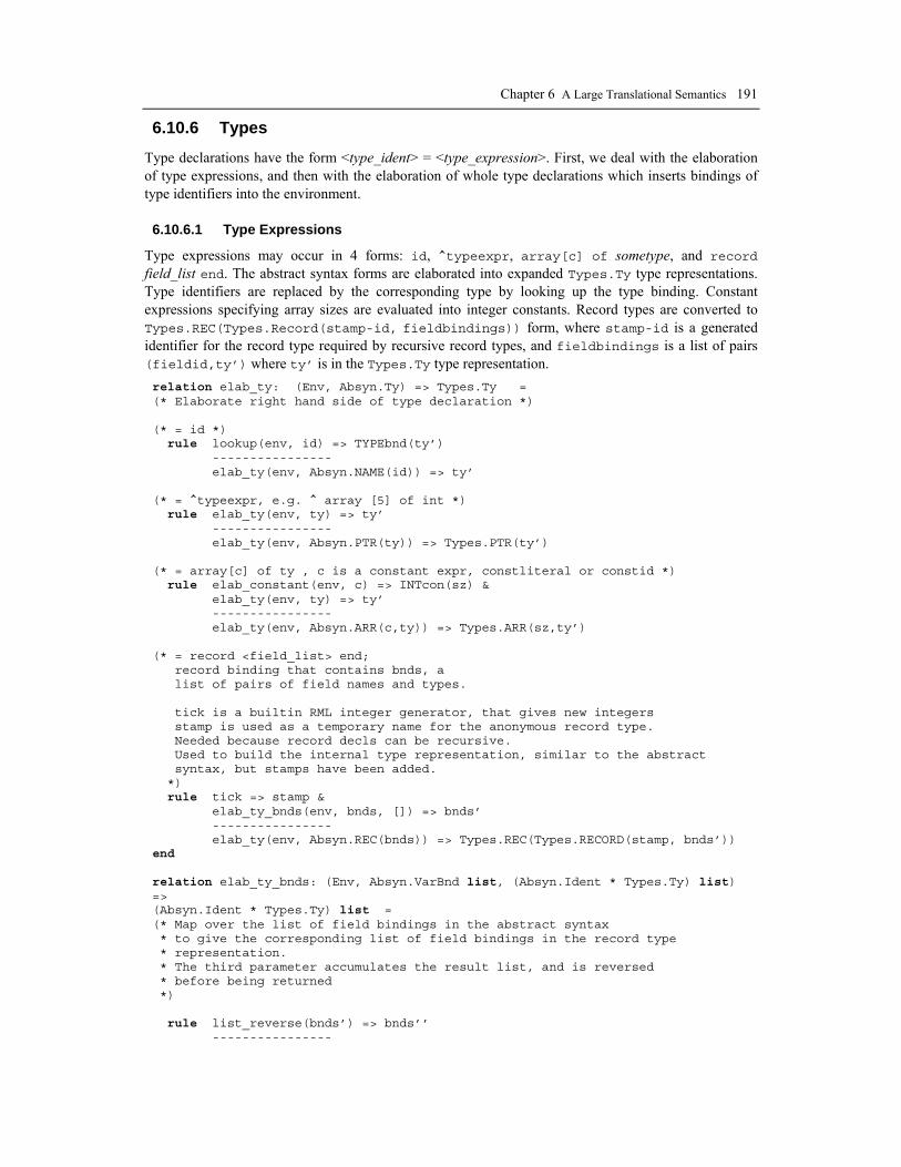
Chapter 6 A Large Translational Semantics 191
6.10.6 Types
Type declarations have the form <type_ident> = <type_expression>. First, we deal with the elaboration of type expressions, and then with the elaboration of whole type declarations which inserts bindings of type identifiers into the environment.
6.10.6.1 Type Expressions
Type expressions may occur in 4 forms: id, ^typeexpr, array[c] of sometype, and record field_list end. The abstract syntax forms are elaborated into expanded Types.Ty type representations. Type identifiers are replaced by the corresponding type by looking up the type binding. Constant expressions specifying array sizes are evaluated into integer constants. Record types are converted to Types.REC(Types.Record(stamp-id, fieldbindings)) form, where stamp-id is a generated identifier for the record type required by recursive record types, and fieldbindings is a list of pairs (fieldid,ty’) where ty’ is in the Types.Ty type representation. relation elab_ty: (Env, Absyn.Ty) => Types.Ty = (* Elaborate right hand side of type declaration *) (* = id *) rule lookup(env, id) => TYPEbnd(ty’) ---------------- elab_ty(env, Absyn.NAME(id)) => ty’ (* = ^typeexpr, e.g. ^ array [5] of int *) rule elab_ty(env, ty) => ty’ ---------------- elab_ty(env, Absyn.PTR(ty)) => Types.PTR(ty’) (* = array[c] of ty , c is a constant expr, constliteral or constid *) rule elab_constant(env, c) => INTcon(sz) & elab_ty(env, ty) => ty’ ---------------- elab_ty(env, Absyn.ARR(c,ty)) => Types.ARR(sz,ty’) (* = record <field_list> end; record binding that contains bnds, a list of pairs of field names and types. tick is a builtin RML integer generator, that gives new integers stamp is used as a temporary name for the anonymous record type. Needed because record decls can be recursive. Used to build the internal type representation, similar to the abstract syntax, but stamps have been added. *) rule tick => stamp & elab_ty_bnds(env, bnds, []) => bnds’ ---------------- elab_ty(env, Absyn.REC(bnds)) => Types.REC(Types.RECORD(stamp, bnds’)) end relation elab_ty_bnds: (Env, Absyn.VarBnd list, (Absyn.Ident * Types.Ty) list) => (Absyn.Ident * Types.Ty) list = (* Map over the list of field bindings in the abstract syntax * to give the corresponding list of field bindings in the record type * representation. * The third parameter accumulates the result list, and is reversed * before being returned *) rule list_reverse(bnds’) => bnds’’ ----------------

192 Peter Fritzson Generation of Language Implementations from Structural and Natural Semantics
elab_ty_bnds(env, [], bnds’) => bnds’’ rule elab_ty(env, ty) => ty’ & elab_ty_bnds(env, bnds, (id,ty’)::bnds’) => bnds’’ ---------------- elab_ty_bnds(env, Absyn.VARBND(id,ty)::bnds, bnds’) => bnds’’ end
6.10.6.2 Type Declarations
The function elab_types analyzes a list of type declaration in abstract syntax form, e.g. TYPE foo=x,y=integer. It calls elab_tybnd to elaborate each type declaration and create type bindings which are pushed on the environment. relation elab_types: (Env, Absyn.TyBnd list) => Env = axiom elab_types(env, []) => env rule elab_tybnd(env, tybnd) => env' & elab_types(env', tybnds) => env'' ---------------- elab_types(env, tybnd::tybnds) => env'' end
Relation elab_tybnd pushes a type binding on the environment. It first calls isrec to mark it as record or no record, then calls elab_tybnd’ to elaborate the type, specially handling recursive records, and finally pushes the binding on the environment. relation elab_tybnd: (Env, Absyn.TyBnd) => Env = rule isrec ty => xxx & elab_tybnd'(xxx, env0, id) => ty' ---------------- elab_tybnd(env0, Absyn.TYBND(id,ty)) => ((id,TYPEbnd(ty'))::env0) end
Relation elab_tybnd’ returns the elaborated type of the declaration in Types.Ty form. For a record declaration some special handling is needed since it may recursively refer to itself. Therefore, a temporary record name stamp generated by calling tick, embedded in
UNFOLD(stamp) is temporarily bound to the record id in the environment passed to elab_ty_bnds, which will recursively traverse field bindings and replace recursive record references by UNFOLD nodes.
For example, in the following record type declaration: type foo = record elem:integer; next: ^foo end;
the recursive type reference to foo is replaced by UNFOLD(stamp) as in the Types.Ty type representation below where stamp happens to be 27: REC(RECORD(27, [(elem, ARITH(INT)), (next, PTR(UNFOLD(27))] ))
The relation elab_tybnd’ follows below: relation elab_tybnd': (IsRec,Env,Ident) => Types.Ty = rule tick => stamp & elab_ty_bnds((id,TYPEbnd(Types.UNFOLD(stamp)))::env0,bnds,[]) => bnds' & check_bnds(bnds') ---------------- elab_tybnd'(ISREC(bnds),env0,id) =>Types.REC(Types.RECORD(stamp,bnds')) (* If no record, cannot be recursive, just return elaborated type *) rule elab_ty(env0, ty) => ty' ---------------- elab_tybnd'(NOREC(ty), env0, id) => ty' end
Relation check_bnds checks a list of field bindings that recursive record type references (UNFOLD) may only occur after a pointer (PTR). If this is not the case, it fails. This means that:

Chapter 6 A Large Translational Semantics 193
type t = record foo: integer; next: ^t end;
is OK, but: type t = record foo: integer; next: t end;
would not be correct. Relations check_bnds and check_ty call each other recursively during this process.
relation check_bnds: (Ident, Types.Ty) list => () = axiom check_bnds [] rule check_ty ty & check_bnds bnds ---------------- check_bnds((_,ty)::bnds) end
Recursively traverse the type representation to check that recursive record references, represented by UNFOLD, are always preceded by a pointer (PTR). If this is not the case, it fails. relation check_ty: Types.Ty => ()= axiom check_ty(Types.ARITH(_)) rule check_ty ty ---------------- check_ty(Types.ARR(_,ty)) rule check_bnds bnds ---------------- check_ty(Types.REC(Types.RECORD(_,bnds))) (* require that UNFOLD is preceeded by PTR *) rule isunfold ty => true ---------------- check_ty(Types.PTR(ty)) rule isunfold ty => false & check_ty ty ---------------- check_ty(Types.PTR(ty)) end
The relation isunfold returns true for UNFOLD nodes and false for all other Types.Ty nodes. relation isunfold: Types.Ty => bool = axiom isunfold(Types.UNFOLD(_)) => true axiom isunfold(Types.ARITH(_)) => false axiom isunfold(Types.PTR(_)) => false axiom isunfold(Types.ARR(_,_)) => false axiom isunfold(Types.REC(_)) => false end
The relation isrec(ty) tests whether ty is an abstract syntax record node, in which case it returns the marker ISREC(bnds). Otherwise, i.e., for a name, pointer, or array, it returns NOREC(ty). relation isrec: Absyn.Ty => IsRec = axiom isrec(ty as Absyn.NAME(_)) => NOREC(ty) axiom isrec(ty as Absyn.PTR(_)) => NOREC(ty) axiom isrec(ty as Absyn.ARR(_,_)) => NOREC(ty) axiom isrec(Absyn.REC(bnds)) => ISREC(bnds) end

194 Peter Fritzson Generation of Language Implementations from Structural and Natural Semantics
6.10.7 Expressions
Expressions occur in two contexts. In r-value context, the expression should yield a value when evaluated, as in the right hand side of assignment statements or in many other situations. In l-value context, the expression should yield an address (or similar) to some location in which a value can be stored. Examples of r-value expressions: x, (a+b), sin(b)-p^, and of l-value expressions: x, p^, p^.b.
The function that translates all r-value expressions to TCode is elab_rvalue, whereas elab_lvalue translates all possible l-value expressions.
6.10.7.1 R-value Expressions
The relation elab_rvalue is the top-most function that translates all possible r-value expressions to pairs consisting of a TCode expression and its associated type. This type is needed for further type checking and type inference.
Relation elab_rvalue contains one rule for each node type in Absyn.Exp. An occurrence of a single identifier id is looked up in the environment to obtain its binding, and translated by calling rvalue_id.
A record field reference is handled by relations elab_field and elab_rvalue_var. Operator nodes (unary, binary, or relational) are translated in two stages, where the details of unary
nodes are taken care of by elab_unary_rvalue. First the argument expression types are decayed, i.e., converted to more primitive types closer to the target machine. For example CHAR is converted to INT, and ARR is converted to PTR. At the same time the corresponding argument expression is translated to TCode. All this is handled by elab_rvalue_decay. The next step, performed by Types.bin_cnv or Types.rel_cnv, is to insert appropriate type conversions of expression arguments and to translate the binary or relational operator to the corresponding typed TCode operator. For example, in binary operator applications such as: INT binop REAL, a conversion from integer to real should be inserted for the first argument expression to make it possible to use the real version of binop. Note that the boolean result of a relational operator is decayed to an integer representation in TCode. relation elab_rvalue: (Env, Absyn.Exp) => (TCode.Exp, Types.Ty) =
axiom elab_rvalue(env, Absyn.INT(i)) => (TCode.ICON(i),Types.ARITH(Types.INT)) axiom elab_rvalue(env,Absyn.REAL(r))=>(TCode.RCON(r), Types.ARITH(Types.REAL)) rule lookup(env, id) => bnd & rvalue_id(bnd, id) => (exp, ty) ---------------- (* id *) elab_rvalue(env, Absyn.IDENT(id)) => (exp, ty) rule elab_rvalue_decay(env, exp) => (exp’, ty’) & elab_ty(env, ty) => ty’’ & Types.cast_cnv(exp’, ty’, ty’’) => exp’’ ---------------- (* type cast *) elab_rvalue(env,Absyn.CAST(ty,exp)) => (exp’’, ty’’) rule elab_field(env, exp, id) => (exp’, ty) & rvalue_var(ty, exp’) => (exp’’, ty’) ---------------- (* fieldref: exp.id *) elab_rvalue(env,Absyn.FIELD(exp,id)) => (exp’’, ty’) rule elab_unary_rvalue(env, unop, exp) => (exp’, rty) ---------------- (* unop exp *) elab_rvalue(env, Absyn.UNARY(unop,exp)) => (exp’, rty) rule elab_rvalue_decay(env, exp1) => (exp1’, rty1) & elab_rvalue_decay(env, exp2) => (exp2’, rty2) & Types.bin_cnv(exp1’, rty1, binop, exp2’, rty2) => (exp3, rty3) ---------------- (* exp1 binop exp2 *)
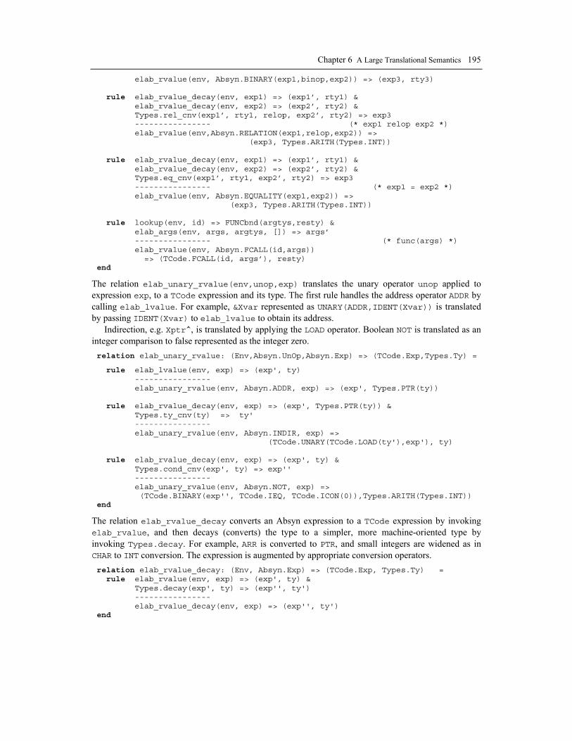
Chapter 6 A Large Translational Semantics 195
elab_rvalue(env, Absyn.BINARY(exp1,binop,exp2)) => (exp3, rty3) rule elab_rvalue_decay(env, exp1) => (exp1’, rty1) & elab_rvalue_decay(env, exp2) => (exp2’, rty2) & Types.rel_cnv(exp1’, rty1, relop, exp2’, rty2) => exp3 ---------------- (* exp1 relop exp2 *) elab_rvalue(env,Absyn.RELATION(exp1,relop,exp2)) => (exp3, Types.ARITH(Types.INT)) rule elab_rvalue_decay(env, exp1) => (exp1’, rty1) & elab_rvalue_decay(env, exp2) => (exp2’, rty2) & Types.eq_cnv(exp1’, rty1, exp2’, rty2) => exp3 ---------------- (* exp1 = exp2 *) elab_rvalue(env, Absyn.EQUALITY(exp1,exp2)) => (exp3, Types.ARITH(Types.INT)) rule lookup(env, id) => FUNCbnd(argtys,resty) & elab_args(env, args, argtys, []) => args’ ---------------- (* func(args) *) elab_rvalue(env, Absyn.FCALL(id,args)) => (TCode.FCALL(id, args’), resty) end
The relation elab_unary_rvalue(env,unop,exp) translates the unary operator unop applied to expression exp, to a TCode expression and its type. The first rule handles the address operator ADDR by calling elab_lvalue. For example, &Xvar represented as UNARY(ADDR,IDENT(Xvar)) is translated by passing IDENT(Xvar) to elab_lvalue to obtain its address.
Indirection, e.g. Xptr^, is translated by applying the LOAD operator. Boolean NOT is translated as an integer comparison to false represented as the integer zero. relation elab_unary_rvalue: (Env,Absyn.UnOp,Absyn.Exp) => (TCode.Exp,Types.Ty) =
rule elab_lvalue(env, exp) => (exp', ty) ---------------- elab_unary_rvalue(env, Absyn.ADDR, exp) => (exp', Types.PTR(ty)) rule elab_rvalue_decay(env, exp) => (exp', Types.PTR(ty)) & Types.ty_cnv(ty) => ty' ---------------- elab_unary_rvalue(env, Absyn.INDIR, exp) => (TCode.UNARY(TCode.LOAD(ty'),exp'), ty) rule elab_rvalue_decay(env, exp) => (exp', ty) & Types.cond_cnv(exp', ty) => exp'' ---------------- elab_unary_rvalue(env, Absyn.NOT, exp) => (TCode.BINARY(exp'', TCode.IEQ, TCode.ICON(0)),Types.ARITH(Types.INT)) end
The relation elab_rvalue_decay converts an Absyn expression to a TCode expression by invoking elab_rvalue, and then decays (converts) the type to a simpler, more machine-oriented type by invoking Types.decay. For example, ARR is converted to PTR, and small integers are widened as in CHAR to INT conversion. The expression is augmented by appropriate conversion operators. relation elab_rvalue_decay: (Env, Absyn.Exp) => (TCode.Exp, Types.Ty) = rule elab_rvalue(env, exp) => (exp', ty) & Types.decay(exp', ty) => (exp'', ty') ---------------- elab_rvalue_decay(env, exp) => (exp'', ty') end
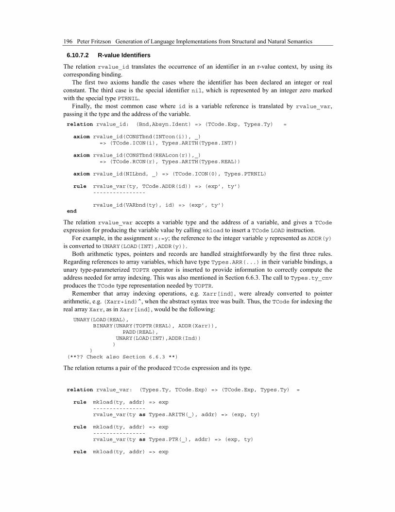
196 Peter Fritzson Generation of Language Implementations from Structural and Natural Semantics
6.10.7.2 R-value Identifiers
The relation rvalue_id translates the occurrence of an identifier in an r-value context, by using its corresponding binding.
The first two axioms handle the cases where the identifier has been declared an integer or real constant. The third case is the special identifier nil, which is represented by an integer zero marked with the special type PTRNIL.
Finally, the most common case where id is a variable reference is translated by rvalue_var, passing it the type and the address of the variable. relation rvalue_id: (Bnd,Absyn.Ident) => (TCode.Exp, Types.Ty) = axiom rvalue_id(CONSTbnd(INTcon(i)), _) => (TCode.ICON(i), Types.ARITH(Types.INT)) axiom rvalue_id(CONSTbnd(REALcon(r)),_) => (TCode.RCON(r), Types.ARITH(Types.REAL)) axiom rvalue_id(NILbnd, _) => (TCode.ICON(0), Types.PTRNIL) rule rvalue_var(ty, TCode.ADDR(id)) => (exp’, ty’) ---------------- rvalue_id(VARbnd(ty), id) => (exp’, ty’) end
The relation rvalue_var accepts a variable type and the address of a variable, and gives a TCode expression for producing the variable value by calling mkload to insert a TCode LOAD instruction.
For example, in the assignment x:=y; the reference to the integer variable y represented as ADDR(y) is converted to UNARY(LOAD(INT),ADDR(y)).
Both arithmetic types, pointers and records are handled straightforwardly by the first three rules. Regarding references to array variables, which have type Types.ARR(...) in their variable bindings, a unary type-parameterized TOPTR operator is inserted to provide information to correctly compute the address needed for array indexing. This was also mentioned in Section 6.6.3. The call to Types.ty_cnv produces the TCode type representation needed by TOPTR.
Remember that array indexing operations, e.g. Xarr[ind], were already converted to pointer arithmetic, e.g. (Xarr+ind)^, when the abstract syntax tree was built. Thus, the TCode for indexing the real array Xarr, as in Xarr[ind], would be the following: UNARY(LOAD(REAL), BINARY(UNARY(TOPTR(REAL), ADDR(Xarr)), PADD(REAL), UNARY(LOAD(INT),ADDR(Ind)) ) ) (**?? Check also Section 6.6.3 **)
The relation returns a pair of the produced TCode expression and its type.
relation rvalue_var: (Types.Ty, TCode.Exp) => (TCode.Exp, Types.Ty) = rule mkload(ty, addr) => exp ---------------- rvalue_var(ty as Types.ARITH(_), addr) => (exp, ty) rule mkload(ty, addr) => exp ---------------- rvalue_var(ty as Types.PTR(_), addr) => (exp, ty) rule mkload(ty, addr) => exp
Chapter 6 A Large Translational Semantics 197
---------------- rvalue_var(ty as Types.REC(_), addr) => (exp, ty) rule Types.ty_cnv(ty) => ty’ ---------------- rvalue_var(Types.ARR(_,ty), addr) => (TCode.UNARY(TCode.TOPTR(ty’), addr), Types.PTR(ty)) end
The relation mkload de-references a pointer (i.e., address expression) by inserting a type-specific LOAD instruction. Different types may occur, e.g. integer, real, record, etc. The call to Types.ty_cnv is to convert the type to the TCode type representation used in the type parameterized LOAD instruction. relation mkload: (Types.Ty,TCode.Exp) => TCode.Exp = rule Types.ty_cnv(ty) => ty' ---------------- mkload(ty, addr) => TCode.UNARY(TCode.LOAD(ty'), addr) end
6.10.7.3 Argument Assignment Conversion
As already mentioned in the short overview, Section 6.10.1, assignment conversion is often needed when assigning actual argument expressions to formal parameters. For example, an integer expression must be converted to real, before being assigned to a real formal parameter.
The relation elab_args(env,exp,ty) performs assignment conversion for a single actual argument expression exp to be converted to the formal parameter type ty. relation elab_arg: (Env,Absyn.Exp,Types.Ty) => TCode.Exp = rule elab_rvalue(env, exp) => (exp', ty') & Types.asg_cnv(exp', ty', ty) => exp'' ---------------- elab_arg(env, exp, ty) => exp'' end
The relation elab_args(env,exps,tys,exps’) performs assignment conversion for a list of arguments exps according to a list of parameter types tys. The converted expressions are accumulated in exps’ and reversed into the correct order before being returned as args''. relation elab_args: (Env, Absyn.Exp list, Types.Ty list, TCode.Exp list) => TCode.Exp list = rule list_reverse(args') => args'' ---------------- elab_args(_, [], [], args') => args'' rule elab_arg(env, exp, ty) => exp' & elab_args(env, exps, tys, exp'::exps') => exps'' ---------------- elab_args(env, exp::exps, ty::tys, exps') => exps'' end
6.10.7.4 L-value Expressions
L-value expressions are expressions that occur in a context where a value should be stored at a location represented by the expression. The relation elab_lvalue(env,exp) computes the address of exp, and its type in l-value context. For example, an expression consisting of the integer variable Ivar would give the result pair (TCode.ADDR(Ivar), ARITH(INT)). Note that because of the l-value context, the type does not contain a PTR operator even though there is an address operator on the variable. We are storing into an integer variable, not assigning a pointer variable. Thus, one pointer level is removed in the resulting type.
198 Peter Fritzson Generation of Language Implementations from Structural and Natural Semantics
The three cases to be taken care of are variable, record field and pointed value assignment, as in the example below: x := ... xrec.field := ... ptr^ := ...
These three cases are handled by the corresponding three rules in elab_lvalue. The third case also covers assignment of array elements, since expressions like Xarr[ind] have been converted to (Xarr+ind)^ using pointer arithmetic. Type decay is only needed in the third case, where possible array types are converted to pointers. relation elab_lvalue: (Env,Absyn.Exp) => (TCode.Exp, Types.Ty) = rule lookup(env, id) => VARbnd(ty) ---------------- elab_lvalue(env, Absyn.IDENT(id)) => (TCode.ADDR(id), ty) rule elab_field(env, exp, id) => (exp’, ty) ---------------- elab_lvalue(env, Absyn.FIELD(exp,id)) => (exp’, ty) rule elab_rvalue_decay(env, exp) => (exp’, Types.PTR(ty)) ---------------- elab_lvalue(env, Absyn.UNARY(Absyn.INDIR,exp)) => (exp’, ty) end
6.10.7.5 Record Fields
The relation elab_field(env,exp,id) elaborates the record expression exp with field id into a TCode l-value address expression of the record field, and its type.
First elaborate exp by calling elab_lvalue to get the address of the record itself, and its type. Then call Types.unfold_rec to unfold the record type one level and return bnds, i.e., a list of pairs (field-id, field-type). Then lookup the field-id to obtain its type, and check that it is declared in the record. Then call Types.rec_cnv to convert from the Types representation to the TCode type representation. Finally insert a unary OFFSET operator to compute the address of the field. As an example, regarding the record variable foo: var foo: record x:integer; b:real end;
the field reference foo.x would be translated to the following TCode, with a record type stamp 33: UNARY(OFFSET(RECORD(33,[(x,INT),(b,REAL)]), x), ADDR(foo))
and the obtained field type ty being ARITH(INT) in the Types.Ty representation. relation elab_field: (Env, Absyn.Exp, Absyn.Ident) => (TCode.Exp, Types.Ty) =
rule elab_lvalue(env, exp) => (exp’, Types.REC(r)) & Types.unfold_rec r => bnds & lookup’(bnds, id) => ty & Types.rec_cnv(r) => r’ ---------------- elab_field(env, exp, id) => (TCode.UNARY(TCode.OFFSET(r’,id),exp’), ty) end
6.10.8 Statements
The relation elab_stmt(fty,env,stmt) translates all Petrol statement types, passed as stmt, and an optional function type fty passed for statements that occur in a function body since the function return

Chapter 6 A Large Translational Semantics 199
expression need to be type checked. The Petrol Abstract syntax of statements (Section 6.5), is shown again below: datatype Absyn.Stmt = ASSIGN of Exp * Exp | PCALL of Ident * Exp list | FRETURN of Exp | PRETURN | WHILE of Exp * Stmt | IF of Exp * Stmt * Stmt | SEQ of Stmt * Stmt | SKIP
which is very close to the TCode statement representation (Section 6.6.5): datatype TCode.Stmt = STORE of Ty * Exp * Exp | PCALL of Ident * Exp list | RETURN of (Ty * Exp) option | WHILE of Exp * Stmt | IF of Exp * Stmt * Stmt | SEQ of Stmt * Stmt | SKIP
The only visible differences are that the assignment has been replaced by a STORE node where the stored type is explicit, and that function and procedure returns have been unified into a single return with optional return type and expression. More detailed comments follow below at specific rules, but first the signature of the relation is presented: relation elab_stmt: (Types.Ty option, Env, Absyn.Stmt) => TCode.Stmt =
Regarding translation of an assignment statement, elaboration of the left hand side is done in l-value context and of the right hand side in r-value context, also obtaining the left hand type as lvalty and the right hand type as rvalty. Then assignment conversion is done on the right hand expression (rval) to obtain the same type as the left hand side. Finally, Types.ty_cnv converts the type into the TCode type representation needed by the STORE node. rule elab_lvalue(env, lhs) => (lval, lvalty) & elab_rvalue(env, rhs) => (rval, rvalty) & Types.asg_cnv(rval, rvalty, lvalty) => rval' & Types.ty_cnv(lvalty) => lvalty' ---------------- (* lhs := rhs; *) elab_stmt(fty, env, Absyn.ASSIGN(lhs,rhs)) => TCode.STORE(lvalty',lval,rval')
A procedure call is translated by first looking up the procedure binding, and then elaborating the arguments including performing assignment conversion. rule lookup(env, id) => PROCbnd(argtys) & elab_args(env, args, argtys, []) => args' ---------------- (* procid(args); *) elab_stmt(fty, env, Absyn.PCALL(id,args)) => TCode.PCALL(id, args')
A function return is translated by elaborating the return expression to TCode, then doing assignment conversion to the function return type, and finally converting the return type to the TCode type representation.
The pattern SOME(rty), means that the return type is optional but is present here as always for function returns. The alternative pattern NONE, used for procedure return, means that the return type is not present. Both SOME and NONE are constructors in the pre-defined option type generator. rule elab_rvalue(env, exp) => (exp', ety) & Types.asg_cnv(exp', ety, rty) => exp'' & Types.ty_cnv(rty) => rty' ---------------- (* return expr *) elab_stmt(SOME(rty),env,Absyn.FRETURN(exp))

200 Peter Fritzson Generation of Language Implementations from Structural and Natural Semantics
=> TCode.RETURN(SOME((rty',exp'')))
A procedure return, indicated by no return type (NONE), is just converted to TCode.RETURN. axiom elab_stmt(NONE, env, Absyn.PRETURN) => TCode.RETURN(NONE) (* return *)
Regarding the while statement in the Petrol language, the predicate expression exp is not required to be of boolean type as in e.g. standard Pascal. Instead, just as in C, all primitive types are allowed. A non-zero value is interpreted as true, and a zero value as false. For example, while 0.0 do ... has the same semantics as while false do ...
The expression is first decayed to primitive types (e.g. char to integer). The Types.cond_cnv relation converts the expression exp in boolean context to a comparison, e.g. converting (xfloat-1) to (xfloat-1)<>0.0 or converting xptr to xptr<>nil. Finally, the while-statement body stmt is elaborated the usual way. rule elab_rvalue_decay(env, exp) => (exp', ety) & Types.cond_cnv(exp', ety) => exp'' & elab_stmt(fty, env, stmt) => stmt' ---------------- (* while exp do stmt *) elab_stmt(fty, env, Absyn.WHILE(exp,stmt)) => TCode.WHILE(exp'', stmt')
The first two steps in the translation of an if-statement is the same as for the while-statement. First the predicate exp is translated to TCode and decayed to a possibly simpler type. Then predicate conversion to a comparison is performed (as for the while-statement). Finally, both the then-part (stmt1) and the else-part (stmt2) are translated, and a TCode.if node is built. rule elab_rvalue_decay(env, exp) => (exp', ety) & Types.cond_cnv(exp', ety) => exp'' & elab_stmt(fty, env, stmt1) => stmt1' & elab_stmt(fty, env, stmt2) => stmt2' ---------------- (* if exp then stmt1 else stmt2 end *) elab_stmt(fty,env,Absyn.IF(exp,stmt1,stmt2)) => TCode.IF(exp'',stmt1',stmt2')
A sequence of statements is translated simply by elaborating the individual statements and constructing a corresponding TCode sequence of the translated statements. rule elab_stmt(fty, env, stmt1) => stmt1' & elab_stmt(fty, env, stmt2) => stmt2' ---------------- (* stmt1; stmt2 *) elab_stmt(fty, env, Absyn.SEQ(stmt1,stmt2)) => TCode.SEQ(stmt1', stmt2')
An empty statement in abstract syntax form (SKIP) just becomes a corresponding TCode.SKIP node. axiom elab_stmt(fty, env, Absyn.SKIP) => TCode.SKIP (* empty stmt ; *) end
6.10.9 Variable and Sub-Program Declarations
Declarations have the effect of associating information with declared identifiers by inserting bindings in an environment structure, as described in Section 6.8. Additionally, functions and procedures also give rise to translated code. The translation of functions, procedures, and blocks was already described in detail in the overview Section 6.10.1. The elaboration of constants and constant declarations was described in Section 6.10.5, and the elaboration of types and type declarations in Section 6.10.6.
Therefore we just provide complementary information regarding the elaboration of variables and formal parameters in this section.
Chapter 6 A Large Translational Semantics 201
6.10.9.1 Variable Declarations
The top level functions in this section called from elsewhere are elab_vars, mkbnd, and mkvarbnd, called by elab_formals and elab_block,
The relation elab_vars elaborates a list of variable or formal parameter bindings (Absyn.VARBND) into a list of pairs (id,ty), where ty is in the Types.Ty representation. However, updating the environment is handled elsewhere by elab_block, which calls elab_vars. The first rule just reverses the list of pairs which has been accumulated in vars’ by the second rule. relation elab_vars: (Env, Absyn.VarBnd list, (Absyn.Ident,Types.Ty) list) => (Absyn.Ident,Types.Ty) list = rule list_reverse(vars') => vars'' ---------------- elab_vars(_, [], vars') => vars'' rule elab_var(env, var) => (id,ty) & elab_vars(env, vars, (id,ty)::vars') => vars'' ---------------- elab_vars(env, var::vars, vars') => vars'' end
The relation elab_var accepts an environment and an abstract syntax variable or formal parameter binding and returns a pair of values id and ty, where ty has been elaborated by elab_ty into the Types.Ty representation and type aliases have been removed, as described in Section 6.10.6. relation elab_var: (Env,Avsyn.VarBnd) => (Absyn.Ident,Types.Ty) = rule elab_ty(env, ty) => ty' ---------------- elab_var(env, Absyn.VARBND(id,ty)) => (id,ty') end
Relation mkvar accepts a pair (id,ty) as a tuple and creates a tagged TCode.VAR(id,ty’) pair, which will be used in the Var list of a TCode.BLOCK node, and where the type ty’ has been converted into the TCode type representation by Types.ty_cnv. Since the single input parameter to mkvar is of tuple type and not two separate parameter types, the input parameter type becomes the tuple type Ident * Types.Ty. relation mkvar: (Ident * Types.Ty) => TCode.Var = rule Types.ty_cnv(ty) => ty' ---------------- mkvar((id,ty)) => TCode.VAR(id,ty') end
Relation mkvarbnd adds a VARbnd tag to type ty in an (id,ty) pair represented as a tuple, to differ from constant binding (CONbnd), type binding (TYPEbnd) and other bindings when inserted into the environment. Note that the single result of mkvarbnd is of tuple type, and that double parenthesis syntax is used for the result to differ from the case of several output results. relation mkvarbnd: (Ident * Types.Ty) => (Ident * Static.Bnd) = axiom mkvarbnd((id,ty)) => ((id, VARbnd(ty))) end
6.10.9.2 Formal Parameters
The relation elab_formals(env,formals), called by elab_subbnd, elaborates formal parameters of procedures and functions.
First, the abstract syntax representation of the parameter list formals is elaborated into pre_formals, in which the parameter types are decayed (only converting ARR to PTR), giving the list pre_formals’ used as input for the three parts of the result.
The relation produces a triple (formals’,argenv,argtys), where formals’ is a list of TCode.Var(id,type) nodes produced by mkvar to be used as part of a TCode.PROC node, argenv is

202 Peter Fritzson Generation of Language Implementations from Structural and Natural Semantics
a list of (id,VARbnd(ty)) pairs (tuples) to be inserted into the environment by elab_subbnd, and argtys is a list of the formal parameter types to be used as part of the corresponding function/procedure descriptor which will be inserted into the environment by elab_subbnd. relation elab_formals: (Env, Absyn.VarBnd list) => (TCode.Var list, (Ident * Bnd) list, Types.Ty list) = rule elab_vars(env, formals, []) => pre_formals & map(decay_formal, pre_formals) => pre_formals' & map(mkvar, pre_formals') => formals' & map(mkvarbnd, pre_formals') => argenv & map(extract_ty, pre_formals') => argtys ---------------- elab_formals(env, formals) => (formals', argenv, argtys) end
The relation decay_formal_ty performs type decay of the formal parameter types. Array parameters are represented as pointers, otherwise there is no change. relation decay_formal_ty: Types.Ty => Types.Ty = axiom decay_formal_ty(Types.ARR(_,ty)) => Types.PTR(ty) axiom decay_formal_ty(ty as Types.ARITH(_)) => ty axiom decay_formal_ty(ty as Types.PTR(_)) => ty axiom decay_formal_ty(ty as Types.REC(_)) => ty end
Decay the type ty part of an (id,ty) formal parameter tuple pair, producing a pair where the type has been decayed. relation decay_formal: (Ident * Types.Ty) => (Ident * Types.Ty) = rule decay_formal_ty(ty) => ty' ---------------- decay_formal((id,ty)) => ((id,ty')) end
Extract the type ty from an (id,ty) tuple pair. relation extract_ty: (Ident * Types.Ty) => Types.Ty = axiom ((_,y)) => y end
6.10.9.3 Sub-Programs and Blocks
The relation elab_subbnd translates a function/procedure into TCode and inserts a function/procedure binding in the environment, as is described in detail in Section 6.10.1. relation elab_subbnd: (Env, Absyn.SubBnd) => (Env, TCode.Proc) = (* elaborate a function *) rule elab_ty(env0, ty) => ty0 & decay_formal_ty(ty0) => ty1 & (* ret ARR ==> ret PTR *) Types.ty_cnv(ty1) => ty2 & elab_formals(env0, formals) => (formals’, argenv, argtys) & let env1 = (id, FUNCbnd(argtys,ty1))::env0 & list_append(argenv, env1) => env2 & elab_body(SOME(ty1), env2, block) => block’ ---------------- elab_subbnd(env0, Absyn.FUNCBND(id,formals,ty,block)) => (env1, TCode.PROC(id,formals’,SOME(ty2),block’)) (* elaborate a procedure *) rule elab_formals(env0, formals) => (formals’, argenv, argtys) & let env1 = (id, PROCbnd(argtys))::env0 &

Chapter 6 A Large Translational Semantics 203
list_append(argenv, env1) => env2 & elab_body(NONE, env2, block) => block’ ---------------- elab_subbnd(env0, Absyn.PROCBND(id,formals,block)) => (env1, TCode.PROC(id,formals’,NONE,block’)) end
The relation elab_subbnds elaborates a list of subprogram declarations, giving an updated environment and a list of TCode.PROC nodes representing translated subprograms. relation elab_subbnds: (Env, Absyn.SubBnd list, TCode.Proc list) => (Env, TCode.Proc list) = rule list_reverse(subbnds’) => subbnds’’ ---------------- elab_subbnds(env, [], subbnds’) => (env,subbnds’’) rule elab_subbnd(env, subbnd) => (env’,subbnd’) & elab_subbnds(env’, subbnds, subbnd’::subbnds’) => (env’’,subbnds’’) ---------------- elab_subbnds(env, subbnd::subbnds, subbnds’) => (env’’,subbnds’’) end
The relation elab_body(fty,env,block) elaborates a function/procedure body, where block is empty (NONE) for extern function/procedure declarations. relation elab_body: (Types.Ty option, TCode.Env, Absyn.Block option) => TCode.Block option = axiom elab_body(_, _, NONE) => NONE rule elab_block(fty, env, block) => block' ---------------- elab_body(fty, env, SOME(block)) => SOME(block') end
The relation elab_block translates the local block of a program, procedure or function, including local declarations and executable body. This is described in detail in Section 6.10.1. relation elab_block: (Types.Ty option, TCode.Env, Absyn.Block) => TCode.Block = rule elab_consts(env0, consts) => env1 & (* also pushes on env *) elab_types(env1, types) => env2 & (* also pushes on env * elab_vars(env2, vars, []) => pre_vars & (* only makes pre_vars alst *) map(mkvar, pre_vars) => vars' & map(mkvarbnd, pre_vars) => varenv & list_append(varenv, env2) => env3 & elab_subbnds(env3, subbnds, []) => (env4,subbnds') & elab_stmt(fty, env4, stmt) => stmt' ---------------- elab_block(fty, env0, Absyn.BLOCK(consts,types,vars,subbnds,stmt)) => TCode.BLOCK(vars', subbnds', stmt') end
The relation elaborate translates a whole program, as described in the introduction to Section 6.10.1. relation elaborate: Absyn.Prog => TCode.Prog = rule elab_block(NONE, env_init, block) => block' ---------------- elaborate(Absyn.PROG(id,block)) => TCode.PROG(id,block') end

204 Peter Fritzson Generation of Language Implementations from Structural and Natural Semantics
6.10.10 Summary
We have presented an overview of the Static module which specifies most aspects of the static semantics of the Petrol language—apart from type elaboration which is specified by the Types module described in Section 6.11.
First, a top-down overview of some aspects of the Static module was given, with emphasis on translation of local blocks, functions and procedures. In this context the environment representation is important, which was described earlier in Section 6.8. A translated program example was included to provide some intuition on how the internal representation before and after translation may appear. Then followed short comments on topics such as statements, expressions, assignment conversion, constants and types.
After this introduction, a complete presentation of the Static module was given. First the module header, the environment and other data structures and needed utility functions appeared. Subsequently, constant expressions and declarations together with type expressions and declarations, were covered. Variable and sub-program declarations followed later at the end of module Static. After the types, a long section on expressions was given, covering topics such as r-value expressions, r-value identifiers, argument assignment conversion, l-value expressions and record fields. Then statements were presented, followed by a concluding section on variable and subprogram declarations, including formal parameters.
6.11 Type Elaboration – the Types Module The Types module describes most aspects of type checking, type analysis, and type conversions of Petrol expressions and type representations. The relations in this module interact closely with the Static module when performing these tasks. In fact, the relations in Types could have been made part of the Static module, but instead were placed into a special Types module in order to keep down the size of modules and describe most type-related in one place.
As already mentioned in Section 6.9, four type representations are used in the Petrol specification:
• Types in declarations are represented by abstract syntax, module Absyn, see Section 6.5. • Types in the TCode intermediate code are part of the TCode definition, module TCode, see
Section 6.6. • Types in the FCode intermediate code are part of the FCode definition, module FCode, see
Section 6.6. • Types used during type analysis as attributes and in bindings which are part of the environment
(the “symbol table”), which are defined here in the Types module.
For clarity, we repeat the diagram over the conversions between the different type representations (previously shown in Figure 6-3).
Absyn.Ty
TCode.Ty
Types.Ty
FCode.Ty
Types in program representations
Types in theenvironment andas type attributes
Chapter 6 A Large Translational Semantics 205
Figure 6-4. The three type representations on the left are used for types occurring in program intermediate forms. The Types.Ty representation is used for types in type attributes during type analysis and to represent types in the environment.
The Types module imports the first two type representations, since it performs conversions between the three representations. The abstract syntax type representation is initially build during parsing, whereas the TCode type representation is used for explicit type information embedded in the TCode emitted by relations in the Static module.
The FCode type representation is identical to TCode and used for explicit type information embedded in the FCode emitted by relations in module Flattening.
The Types.Ty type representation defined in this module is used during type analysis and type conversions, and well as in the environment structure.
6.11.1 Types Module Interface Section
The Types module interface section imports the type representations of Absyn and TCode, defines the Types.Ty type representation, and defines the signatures of a number of relations that are exported to be called from the Static module. The module header follows below: (* types.rml *)
module Types: with "absyn.rml" (* import RelOp and BinOp *) with "tcode.rml"
It is relevant to explain the Types.Ty type representation in the context of this module, even though some of this information was presented earlier in the overview.
The Stamp is a kind of “internal” identifier used to represent recursive record type references, which is explained in detail in Section 6.6.2 and Section 6.10.6.
The ATy type tags (CHAR, INT, REAL) define the arithmetic types referred to by the ARITH node. PTRNIL is a node for representing the special case of a null pointer before type analysis has been
performed to deduce the type that it represents. After this analysis, performed by the Types module, the type will be represented as PTR(any), e.g. in the source code a null pointer can be PTR(INT), PTR(DOUBLE), PTR(CHAR), PTR(PTR(INT)), etc.
A type at an l-value position (the left-hand side of an assignment) can be any type, except a PTRNIL node. PTR, ARR, and REC can only refer to l-value types. UNFOLD is an internal placeholder for recursive references to records, that should never occur outside of a RECORD node. (* Type representation in module Types, used for environments and type analysis *) type Ident = string type Stamp = int datatype ATy = CHAR | INT | REAL datatype Ty = ARITH of ATy | PTR of Ty | PTRNIL | ARR of int * Ty | REC of Record | UNFOLD of Stamp and Record = RECORD of Stamp * (Ident * Ty) list
The signatures of relations which are exported from the Types module are presented below, together with short comments regarding their function. More detailed explanations follow later in conjunction with the relations themselves.
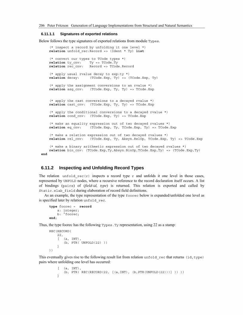
206 Peter Fritzson Generation of Language Implementations from Structural and Natural Semantics
6.11.1.1 Signatures of exported relations
Below follows the type signatures of exported relations from module Types. (* inspect a record by unfolding it one level *) relation unfold_rec:Record => (Ident * Ty) list (* convert our types to TCode types *) relation ty_cnv: Ty => TCode.Ty relation rec_cnv: Record => TCode.Record (* apply usual rvalue decay to exp:ty *) relation decay: (TCode.Exp, Ty) => (TCode.Exp, Ty) (* apply the assignment conversions to an rvalue *) relation asg_cnv: (TCode.Exp, Ty, Ty) => TCode.Exp (* apply the cast conversions to a decayed rvalue *) relation cast_cnv: (TCode.Exp, Ty, Ty) => TCode.Exp (* apply the conditional conversions to a decayed rvalue *) relation cond_cnv: (TCode.Exp, Ty) => TCode.Exp (* make an equality expression out of two decayed rvalues *) relation eq_cnv: (TCode.Exp, Ty, TCode.Exp, Ty) => TCode.Exp (* make a relation expression out of two decayed rvalues *) relation rel_cnv: (TCode.Exp, Ty, Absyn.RelOp, TCode.Exp, Ty) => TCode.Exp (* make a binary arithmetic expression out of two decayed rvalues *) relation bin_cnv: (TCode.Exp,Ty,Absyn.BinOp,TCode.Exp,Ty) => (TCode.Exp,Ty) end
6.11.2 Inspecting and Unfolding Record Types
The relation unfold_rec(r) inspects a record type r and unfolds it one level in those cases, represented by UNFOLD nodes, where a recursive reference to the record declaration itself occurs. A list of bindings (pairs) of (field-id, type) is returned. This relation is exported and called by Static.elab_field during elaboration of record field definitions.
As an example, the type representation of the type foorec below is expanded/unfolded one level as is specified later by relation unfold_rec. type foorec = record a: integer; b: ^foorec; end;
Thus, the type foorec has the following Types.Ty representation, using 22 as a stamp: REC(RECORD( 22, [ (a, INT), (b, PTR( UNFOLD(22) )) ] ))
This eventually gives rise to the following result list from relation unfold_rec that returns (id,type) pairs where unfolding one level has occurred: [ (a, INT), (b, PTR( REC(RECORD(22, [(a,INT), (b,PTR(UNFOLD(22)))] )) )) ]

Chapter 6 A Large Translational Semantics 207
The relation unfold_rec follows: relation unfold_rec: Record => (Ident * Ty) list = rule unfold_bnds(r, bnds, []) => bnds' ---------------- unfold_rec(r as RECORD(stamp, bnds)) => bnds' end
The relation unfold_bnds(bnds) maps unfold_ty on each field binding in the bnds list to perform unfolding one level of the type in the binding represented as a pair (id,type).
The resulting list of pairs is accumulated in bnds’, which is reversed into the original order by the first rule before being returned. relation unfold_bnds: (Record, (Ident * Ty) list, (Ident * Ty) list) => (Ident * Ty) list = rule list_reverse(bnds’) => bnds’’ ---------------- unfold_bnds(_, [], bnds’) => bnds’’ rule unfold_ty(ty, r) => ty’ & unfold_bnds(r, bnds, (id,ty’)::bnds’) => bnds’’ ---------------- unfold_bnds(r, (id,ty)::bnds, bnds’) => bnds’’ end
The relation unfold_ty(ty,r) performs unfolding one level of recursive references in ty. It just copies the type representation of ty, except for recursive references to the record type itself represented by UNFOLD nodes. Each UNFOLD node is replaced by the record r. For nodes such as PTR, ARR and REC(RECORD) the relation calls itself recursively to traverse the type representation. It is called from elsewhere only by unfold_rec and unfold_bnds. relation unfold_ty: (Ty,Record) => Ty =
axiom unfold_ty(ty as ARITH(_), _) => ty axiom unfold_ty(ty as PTRNIL, _) => ty rule unfold_ty(ty, r) => ty' ---------------- unfold_ty(PTR(ty), r) => PTR(ty') rule unfold_ty(ty, r) => ty' ---------------- unfold_ty(ARR(sz,ty), r) => ARR(sz,ty') rule unfold_bnds(r, bnds, []) => bnds' ---------------- unfold_ty(REC(RECORD(stamp,bnds)), r) => REC(RECORD(stamp,bnds')) (* Unfold one level; replace the UNFOLD constructor with a node containing a copy of the record declaration itself *) rule stamp = stamp' ---------------- unfold_ty(UNFOLD(stamp), r as RECORD(stamp',_)) => REC(r) rule not stamp = stamp' ---------------- unfold_ty(ty as UNFOLD(stamp), RECORD(stamp',_)) => ty end

208 Peter Fritzson Generation of Language Implementations from Structural and Natural Semantics
6.11.3 Conversion from Types.Ty to TCode.Ty Type Representation
The relation ty_cnv(ty) converts the type ty from a Types.Ty representation to a corresponding TCode.Ty representation. The conversion is very simple since the two type representations are almost identical, the only change being that ARITH nodes in the Types.Ty representation are eliminated.
The PTRNIL node in the Types.Ty representation is not included, since it is present only temporarily before type inference has been performed. Thus, trying to convert a PTRNIL node here will cause a static type error from the RML system, causing the specification to fail. relation ty_cnv: Ty => TCode.Ty =
axiom ty_cnv(ARITH(CHAR)) => TCode.CHAR axiom ty_cnv(ARITH(INT)) => TCode.INT axiom ty_cnv(ARITH(REAL)) => TCode.REAL rule ty_cnv(ty) => ty' ---------------- ty_cnv(PTR(ty)) => TCode.PTR(ty') rule ty_cnv(ty) => ty' ---------------- ty_cnv(ARR(sz,ty)) => TCode.ARR(sz,ty') rule rec_cnv(r) => r' ---------------- ty_cnv(REC(r)) => TCode.REC(r') axiom ty_cnv(UNFOLD(stamp)) => TCode.UNFOLD(stamp)
end
The relation rec_cnv converts a record type in the Types.Ty form to the corresponding representation in TCode. relation rec_cnv: Record => TCode.Record = rule bnds_cnv(bnds, []) => bnds' ---------------- rec_cnv(RECORD(stamp, bnds)) => TCode.RECORD(stamp, bnds') end
The relation bnds_cnv(bnds) converts the list bnds of field bindings (id,ty) to a corresponding list of binding nodes TCode.Var(id’,ty’) in the TCode representation. relation bnds_cnv: ((Ident * Ty) list, TCode.Var list) => TCode.Var list =
rule list_reverse(bnds') => bnds'' ---------------- bnds_cnv([], bnds') => bnds'' rule ty_cnv(ty) => ty' & bnds_cnv(bnds, TCode.VAR(var,ty')::bnds') => bnds'' ---------------- bnds_cnv((var,ty)::bnds, bnds') => bnds'' end
6.11.4 Type Decay for r-value Expressions
The relation decay(exp,ty) performs type decay, i.e., conversion to simpler, more machine oriented types and expressions. Conversion operators are inserted into the expression exp, and the type ty is converted. However, the expression exp and the type ty are passed unchanged, except for the two cases where CHAR is converted to INT, and array (ARR) expressions are converted to pointer (PTR and TOPTR) expressions and types.
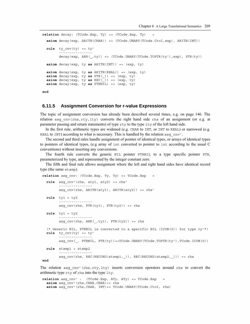
Chapter 6 A Large Translational Semantics 209
relation decay: (TCode.Exp, Ty) => (TCode.Exp, Ty) =
axiom decay(exp, ARITH(CHAR)) => (TCode.UNARY(TCode.CtoI,exp), ARITH(INT)) rule ty_cnv(ty) => ty' ---------------- decay(exp, ARR(_,ty)) => (TCode.UNARY(TCode.TOPTR(ty'),exp), PTR(ty)) axiom decay(exp, ty as ARITH(INT)) => (exp, ty) axiom decay(exp, ty as ARITH(REAL)) => (exp, ty) axiom decay(exp, ty as PTR(_)) => (exp, ty) axiom decay(exp, ty as REC(_)) => (exp, ty) axiom decay(exp, ty as PTRNIL) => (exp, ty) end
6.11.5 Assignment Conversion for r-value Expressions
The topic of assignment conversion has already been described several times, e.g. on page 146. The relation asg_cnv(rhs,rty,lty) converts the right hand side rhs of an assignment (or e.g. at parameter passing and return statements) of type rty to the type lty of the left hand side.
In the first rule, arithmetic types are widened (e.g. CHAR to INT, or INT to REAL) or narrowed (e.g. REAL to INT) according to what is necessary. This is handled by the relation asg_cnv’.
The second and third rules handle assignment of pointer of identical types, or arrays of identical types to pointers of identical types, (e.g array of int converted to pointer to int according to the usual C conventions) without inserting any conversions.
The fourth rule converts the generic NIL pointer PTRNIL to a type specific pointer PTR, parameterized by type, and represented by the integer constant zero.
The fifth and final rule allows assignment where the left and right hand sides have identical record type (the same stamp). relation asg_cnv: (TCode.Exp, Ty, Ty) => TCode.Exp =
rule asg_cnv'(rhs, aty1, aty2) => rhs' ---------------- asg_cnv(rhs, ARITH(aty1), ARITH(aty2)) => rhs' rule ty1 = ty2 ---------------- asg_cnv(rhs, PTR(ty1), PTR(ty2)) => rhs rule ty1 = ty2 ---------------- asg_cnv(rhs, ARR(_,ty1), PTR(ty2)) => rhs (* Generic NIL, PTRNIL is converted to a specific NIL (ICON(0)) for type ty'*) rule ty_cnv(ty) => ty' ---------------- asg_cnv(_, PTRNIL, PTR(ty))=>TCode.UNARY(TCode.TOPTR(ty'),TCode.ICON(0)) rule stamp1 = stamp2 ---------------- asg_cnv(rhs, REC(RECORD(stamp1,_)), REC(RECORD(stamp2,_))) => rhs end
The relation asg_cnv’(rhs,rty,lty) inserts conversion operators around rhs to convert the arithmetic type rty of rhs into the type lty. relation asg_cnv' : (TCode.Exp, ATy, ATy) => TCode.Exp = axiom asg_cnv'(rhs,CHAR,CHAR)=> rhs axiom asg_cnv'(rhs,CHAR, INT)=> TCode.UNARY(TCode.CtoI, rhs)
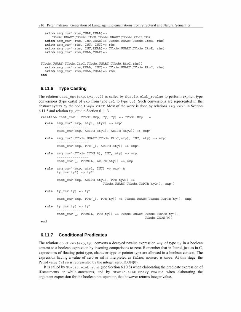
210 Peter Fritzson Generation of Language Implementations from Structural and Natural Semantics
axiom asg_cnv'(rhs,CHAR,REAL)=> TCode.UNARY(TCode.ItoR,TCode.UNARY(TCode.CtoI,rhs)) axiom asg_cnv'(rhs, INT,CHAR)=> TCode.UNARY(TCode.ItoC, rhs) axiom asg_cnv'(rhs, INT, INT)=> rhs axiom asg_cnv'(rhs, INT,REAL)=> TCode.UNARY(TCode.ItoR, rhs) axiom asg_cnv'(rhs,REAL,CHAR)=> TCode.UNARY(TCode.ItoC,TCode.UNARY(TCode.RtoI,rhs)) axiom asg_cnv'(rhs,REAL, INT)=> TCode.UNARY(TCode.RtoI, rhs) axiom asg_cnv'(rhs,REAL,REAL)=> rhs end
6.11.6 Type Casting
The relation cast_cnv(exp,ty1,ty2) is called by Static.elab_rvalue to perform explicit type conversions (type casts) of exp from type ty1 to type ty2. Such conversions are represented in the abstract syntax by the node Absyn.CAST. Most of the work is done by relations asg_cnv’ in Section 6.11.5 and relation ty_cnv in Section 6.11.3. relation cast_cnv: (TCode.Exp, Ty, Ty) => TCode.Exp =
rule asg_cnv’(exp, aty1, aty2) => exp’ ---------------- cast_cnv(exp, ARITH(aty1), ARITH(aty2)) => exp’ rule asg_cnv’(TCode.UNARY(TCode.PtoI,exp), INT, aty) => exp’ ---------------- cast_cnv(exp, PTR(_), ARITH(aty)) => exp’ rule asg_cnv’(TCode.ICON(0), INT, aty) => exp ---------------- cast_cnv(_, PTRNIL, ARITH(aty)) => exp rule asg_cnv’(exp, aty1, INT) => exp’ & ty_cnv(ty2) => ty2’ ---------------- cast_cnv(exp, ARITH(aty1), PTR(ty2)) => TCode.UNARY(TCode.TOPTR(ty2’), exp’) rule ty_cnv(ty) => ty’ ---------------- cast_cnv(exp, PTR(_), PTR(ty)) => TCode.UNARY(TCode.TOPTR(ty’), exp) rule ty_cnv(ty) => ty’ ---------------- cast_cnv(_, PTRNIL, PTR(ty)) => TCode.UNARY(TCode.TOPTR(ty’), TCode.ICON(0)) end
6.11.7 Conditional Predicates
The relation cond_cnv(exp,ty) converts a decayed r-value expression exp of type ty in a boolean context to a boolean expression by inserting comparisons to zero. Remember that in Petrol, just as in C, expressions of floating point type, character type or pointer type are allowed in a boolean context. The expression having a value of zero or nil is interpreted as false; nonzero is true. At this stage, the Petrol value false is represented by the integer zero, ICON(0).
It is called by Static.elab_stmt (see Section 6.10.8) when elaborating the predicate expression of if-statements or while-statements, and by Static.elab_unary_rvalue when elaborating the argument expression for the boolean not-operator, that however returns integer value.
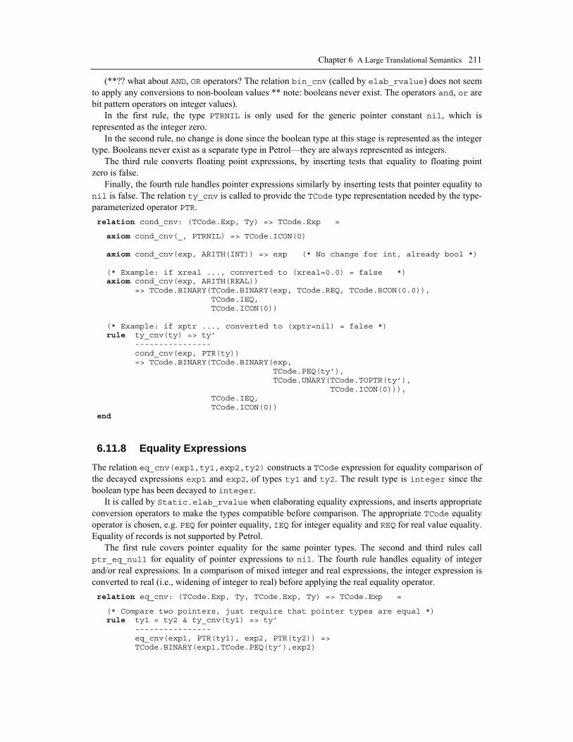
Chapter 6 A Large Translational Semantics 211
(**?? what about AND, OR operators? The relation bin_cnv (called by elab_rvalue) does not seem to apply any conversions to non-boolean values ** note: booleans never exist. The operators and, or are bit pattern operators on integer values).
In the first rule, the type PTRNIL is only used for the generic pointer constant nil, which is represented as the integer zero.
In the second rule, no change is done since the boolean type at this stage is represented as the integer type. Booleans never exist as a separate type in Petrol—they are always represented as integers.
The third rule converts floating point expressions, by inserting tests that equality to floating point zero is false.
Finally, the fourth rule handles pointer expressions similarly by inserting tests that pointer equality to nil is false. The relation ty_cnv is called to provide the TCode type representation needed by the type-parameterized operator PTR. relation cond_cnv: (TCode.Exp, Ty) => TCode.Exp =
axiom cond_cnv(_, PTRNIL) => TCode.ICON(0) axiom cond_cnv(exp, ARITH(INT)) => exp (* No change for int, already bool *) (* Example: if xreal ..., converted to (xreal=0.0) = false *) axiom cond_cnv(exp, ARITH(REAL)) => TCode.BINARY(TCode.BINARY(exp, TCode.REQ, TCode.RCON(0.0)), TCode.IEQ, TCode.ICON(0)) (* Example: if xptr ..., converted to (xptr=nil) = false *) rule ty_cnv(ty) => ty’ ---------------- cond_cnv(exp, PTR(ty)) => TCode.BINARY(TCode.BINARY(exp, TCode.PEQ(ty’), TCode.UNARY(TCode.TOPTR(ty’), TCode.ICON(0))), TCode.IEQ, TCode.ICON(0)) end
6.11.8 Equality Expressions
The relation eq_cnv(exp1,ty1,exp2,ty2) constructs a TCode expression for equality comparison of the decayed expressions exp1 and exp2, of types ty1 and ty2. The result type is integer since the boolean type has been decayed to integer.
It is called by Static.elab_rvalue when elaborating equality expressions, and inserts appropriate conversion operators to make the types compatible before comparison. The appropriate TCode equality operator is chosen, e.g. PEQ for pointer equality, IEQ for integer equality and REQ for real value equality. Equality of records is not supported by Petrol.
The first rule covers pointer equality for the same pointer types. The second and third rules call ptr_eq_null for equality of pointer expressions to nil. The fourth rule handles equality of integer and/or real expressions. In a comparison of mixed integer and real expressions, the integer expression is converted to real (i.e., widening of integer to real) before applying the real equality operator. relation eq_cnv: (TCode.Exp, Ty, TCode.Exp, Ty) => TCode.Exp =
(* Compare two pointers, just require that pointer types are equal *) rule ty1 = ty2 & ty_cnv(ty1) => ty’ ---------------- eq_cnv(exp1, PTR(ty1), exp2, PTR(ty2)) => TCode.BINARY(exp1,TCode.PEQ(ty’),exp2)

212 Peter Fritzson Generation of Language Implementations from Structural and Natural Semantics
(* Special case: compare pointer to nil *) rule ptr_eq_null(exp, ty) => exp’ ---------------- eq_cnv(exp, PTR(ty), _, PTRNIL) => exp’ (* Special case: compare nil to pointer *) rule ptr_eq_null(exp, ty) => exp’ ---------------- eq_cnv(_, PTRNIL, exp, PTR(ty)) => exp’ (* arithmetic case: widen to real if one of them is real *) rule arith_cnv(exp1, raty1, exp2, raty2) => (exp1’, exp2’, raty3) & choose_int_real(raty3, TCode.IEQ, TCode.REQ) => bop ---------------- eq_cnv(exp1, ARITH(raty1), exp2, ARITH(raty2)) => TCode.BINARY(exp1’,bop,exp2’) end
The relation ptr_eq_null(exp,ty) builds an expression to compare the pointer expression exp of pointer type ty to the null pointer. The type ty is converted into the TCode type representation (ty’), which is needed by TOPTR. relation ptr_eq_null: (TCode.Exp, Ty) => TCode.Exp =
rule ty_cnv(ty) => ty' ---------------- ptr_eq_null(exp, ty) => TCode.BINARY(exp,TCode.PEQ(ty'), TCode.UNARY(TCode.TOPTR(ty'),TCode.ICON(0))) end
The relation choose_int_real(aty,iop,rop) chooses the appropriate operator, integer variant iop or real variant rop, depending on the arithmetic type aty. relation choose_int_real: (ATy,TCode.BinOp,TCode.BinOp) => TCode.BinOp = axiom choose_int_real(INT, x, _) => x axiom choose_int_real(REAL, _, y) => y end
The relation arith_cnv(exp1,raty1,exp2,raty2) => (exp1’,exp2’,raty3) inserts appropriate integer to real (ItoR) conversion operators to widen expressions exp1 and exp2 to the common least type upper bound (lub) raty3 of their respective types. For example, the lub of integer and real is real, whereas the lub of integer and integer is integer.
The relation arith_lub computes the lub, whereas arith_widen performs the actual widening of the expressions, giving exp1’ and exp2’. relation arith_cnv: (TCode.Exp,ATy, TCode.Exp,ATy) => (TCode.Exp, TCode.Exp, ATy) = rule arith_lub(raty1, raty2) => raty3 & arith_widen(exp1, raty1, raty3) => exp1' & arith_widen(exp2, raty2, raty3) => exp2' ---------------- arith_cnv(exp1, raty1, exp2, raty2) => (exp1', exp2', raty3) end
The relation arith_lub computes the least upper bound (lub) type of two decayed arithmetic types. For example, the lub of integer and integer is integer, whereas the lub of real and integer or real gives real. relation arith_lub: (ATy, ATy) => ATy = axiom arith_lub(INT, y) => y axiom arith_lub(REAL, _) => REAL end

Chapter 6 A Large Translational Semantics 213
The relation arith_widen(exp,ty1,ty2) widens the decayed arithmetic expression exp by inserting integer to real conversion operators when needed. Since Static.elab_rvalue_decay already has converted the type char to integer, we only need to handle integer and real. relation arith_widen: (TCode.Exp, ATy, ATy) => TCode.Exp = axiom arith_widen(exp, INT, INT) => exp axiom arith_widen(exp, INT, REAL) => TCode.UNARY(TCode.ItoR, exp) axiom arith_widen(exp, REAL, REAL) => exp end
6.11.9 Relational Expressions
The relation rel_cnv(exp1,t1,relop,exp2,t2) translates a relational expression exp1 relop exp2 to an appropriate TCode expression of type integer (representing boolean), where expressions exp1 and exp2 of types t1 and t2 are already in decayed TCode form. Only the relational operators less than (LT) and less then or equal (LE) need to be handled, since GT and GE were eliminated during construction of abstract syntax at parse-time, and equality is handled by eq_cnv.
Two cases of comparison are allowed in Petrol. The first rule covers the case where pointers of identical type are compared: just convert the type to TCode form and call ptr_relop to obtain the correct typed TCode relational operator.
The second case covers comparisons between arithmetic expressions that can be of type either integer or real. The relation arith_cnv inserts widening conversions from integer to real, when integer and real expressions are compared. Selection of the appropriate integer or real relational operator is done by int_or_real_relop. relation rel_cnv: (TCode.Exp, Ty, Absyn.RelOp, TCode.Exp, Ty) => TCode.Exp =
rule ty1 = ty2 & ty_cnv(ty1) => ty' & ptr_relop(relop, ty') => bop ---------------- rel_cnv(exp1,PTR(ty1),relop,exp2,PTR(ty2)) =>TCode.BINARY(exp1,bop,exp2) rule arith_cnv(exp1, raty1, exp2, raty2) => (exp1', exp2', raty3) & int_or_real_relop(raty3, relop) => bop ---------------- rel_cnv(exp1,ARITH(raty1),relop,exp2,ARITH(raty2)) => TCode.BINARY(exp1',bop,exp2') end
The relation ptr_relop performs simple conversions of abstract syntax address comparison operators LT and LE to corresponding pointer operators in TCode. relation ptr_relop: (Absyn.RelOp, Ty) => TCode.BinOp = axiom ptr_relop(Absyn.LT, ty) => TCode.PLT(ty) axiom ptr_relop(Absyn.LE, ty) => TCode.PLE(ty) end
The relation int_or_real_relop(ty,relop) produces the appropriate integer or real TCode variant of the relational operator relop, depending on the type ty. relation int_or_real_relop: (Ty, Absyn.RelOp) => TCode.BinOp = axiom int_or_real_relop(INT, Absyn.LT) => TCode.ILT axiom int_or_real_relop(INT, Absyn.LE) => TCode.ILE axiom int_or_real_relop(REAL, Absyn.LT) => TCode.RLT axiom int_or_real_relop(REAL, Absyn.LE) => TCode.RLE end

214 Peter Fritzson Generation of Language Implementations from Structural and Natural Semantics
6.11.10 Binary Operator Expressions
The relation bin_cnv(exp1,ty1,binop,exp2,ty2) converts a binary arithmetic and/or pointer expression exp1 binop exp2 to a pair (exp3,ty3) of a TCode expression exp3 and its type ty3. The binary operator binop is the abstract syntax (Absyn.BinOp) version whereas the expressions exp1 and exp2 are already in decayed TCode form.
There is one rule for each operator, calling specific conversion relations. There are rules for addition, subtraction, multiplication, real division, integer division, integer modulus, logical integer and, and logical integer or. relation bin_cnv: (TCode.Exp,Ty,Absyn.BinOp,TCode.Exp,Ty) => (TCode.Exp, Ty) =
rule add_cnv(exp1, rty1, exp2, rty2) => (exp3, rty3) ---------------- bin_cnv(exp1, rty1, Absyn.ADD, exp2, rty2) => (exp3, rty3) rule sub_cnv(exp1, rty1, exp2, rty2) => (exp3, rty3) ---------------- bin_cnv(exp1, rty1, Absyn.SUB, exp2, rty2) => (exp3, rty3) rule mul_cnv(exp1, rty1, exp2, rty2) => (exp3, rty3) ---------------- bin_cnv(exp1, rty1, Absyn.MUL, exp2, rty2) => (exp3, rty3) rule rdiv_cnv(exp1, rty1, exp2, rty2) => (exp3, rty3) ---------------- bin_cnv(exp1, rty1, Absyn.RDIV, exp2, rty2) => (exp3, rty3) rule intop_cnv(exp1, rty1, TCode.IDIV, exp2, rty2) => (exp3, rty3) ---------------- bin_cnv(exp1, rty1, Absyn.IDIV, exp2, rty2) => (exp3, rty3) rule intop_cnv(exp1, rty1, TCode.IMOD, exp2, rty2) => (exp3, rty3) ---------------- bin_cnv(exp1, rty1, Absyn.IMOD, exp2, rty2) => (exp3, rty3) rule intop_cnv(exp1, rty1, TCode.IAND, exp2, rty2) => (exp3, rty3) ---------------- bin_cnv(exp1, rty1, Absyn.IAND, exp2, rty2) => (exp3, rty3) rule intop_cnv(exp1, rty1, TCode.IOR, exp2, rty2) => (exp3, rty3) ---------------- bin_cnv(exp1, rty1, Absyn.IOR, exp2, rty2) => (exp3, rty3) end
6.11.10.1 Addition Expressions
The relation add_cnv(exp1,ty1,exp2,ty2) elaborates an addition expression exp1+exp2 into a pair (exp3,ty3) of a resulting TCode expression exp3 and its type ty3. The arguments exp1 and exp2 are r-value expressions in decayed TCode form.
This is a bit complicated since addition of both pointers and arithmetic values, or just arithmetic values are allowed. The result type ty3 is the type of the pointer argument for pointer addition, or a real/integer for arithmetic addition. The appropriate integer (IADD), real (RADD), or pointer version (PADD) of the addition operator is chosen by choose_int_real or ptr_add_int_cnv respectively. The relation arith_cnv—see Section 6.11.8—performs possibly necessary arithmetic widening from integer to real in the third rule. relation add_cnv: (TCode.Exp, Ty, TCode.Exp, Ty) => (TCode.Exp, Ty) =
(* ptr + arith -> ptr *) rule ptr_add_int_cnv(exp1, ty, ty1, exp2) => (exp3, ty3) ----------------
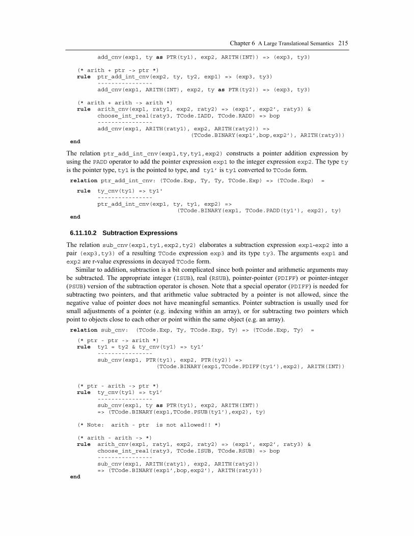
Chapter 6 A Large Translational Semantics 215
add_cnv(exp1, ty as PTR(ty1), exp2, ARITH(INT)) => (exp3, ty3) (* arith + ptr -> ptr *) rule ptr_add_int_cnv(exp2, ty, ty2, exp1) => (exp3, ty3) ---------------- add_cnv(exp1, ARITH(INT), exp2, ty as PTR(ty2)) => (exp3, ty3) (* arith + arith -> arith *) rule arith_cnv(exp1, raty1, exp2, raty2) => (exp1’, exp2’, raty3) & choose_int_real(raty3, TCode.IADD, TCode.RADD) => bop ---------------- add_cnv(exp1, ARITH(raty1), exp2, ARITH(raty2)) => (TCode.BINARY(exp1’,bop,exp2’), ARITH(raty3)) end
The relation ptr_add_int_cnv(exp1,ty,ty1,exp2) constructs a pointer addition expression by using the PADD operator to add the pointer expression exp1 to the integer expression exp2. The type ty is the pointer type, ty1 is the pointed to type, and ty1’ is ty1 converted to TCode form. relation ptr_add_int_cnv: (TCode.Exp, Ty, Ty, TCode.Exp) => (TCode.Exp) =
rule ty_cnv(ty1) => ty1' ---------------- ptr_add_int_cnv(exp1, ty, ty1, exp2) => (TCode.BINARY(exp1, TCode.PADD(ty1'), exp2), ty) end
6.11.10.2 Subtraction Expressions
The relation sub_cnv(exp1,ty1,exp2,ty2) elaborates a subtraction expression exp1-exp2 into a pair (exp3,ty3) of a resulting TCode expression exp3 and its type ty3. The arguments exp1 and exp2 are r-value expressions in decayed TCode form.
Similar to addition, subtraction is a bit complicated since both pointer and arithmetic arguments may be subtracted. The appropriate integer (ISUB), real (RSUB), pointer-pointer (PDIFF) or pointer-integer (PSUB) version of the subtraction operator is chosen. Note that a special operator (PDIFF) is needed for subtracting two pointers, and that arithmetic value subtracted by a pointer is not allowed, since the negative value of pointer does not have meaningful semantics. Pointer subtraction is usually used for small adjustments of a pointer (e.g. indexing within an array), or for subtracting two pointers which point to objects close to each other or point within the same object (e.g. an array). relation sub_cnv: (TCode.Exp, Ty, TCode.Exp, Ty) => (TCode.Exp, Ty) =
(* ptr - ptr -> arith *) rule ty1 = ty2 & ty_cnv(ty1) => ty1’ ---------------- sub_cnv(exp1, PTR(ty1), exp2, PTR(ty2)) => (TCode.BINARY(exp1,TCode.PDIFF(ty1’),exp2), ARITH(INT)) (* ptr - arith -> ptr *) rule ty_cnv(ty1) => ty1’ ---------------- sub_cnv(exp1, ty as PTR(ty1), exp2, ARITH(INT)) => (TCode.BINARY(exp1,TCode.PSUB(ty1’),exp2), ty) (* Note: arith - ptr is not allowed!! *) (* arith - arith -> *) rule arith_cnv(exp1, raty1, exp2, raty2) => (exp1’, exp2’, raty3) & choose_int_real(raty3, TCode.ISUB, TCode.RSUB) => bop ---------------- sub_cnv(exp1, ARITH(raty1), exp2, ARITH(raty2)) => (TCode.BINARY(exp1’,bop,exp2’), ARITH(raty3)) end

216 Peter Fritzson Generation of Language Implementations from Structural and Natural Semantics
6.11.10.3 Multiplication Expressions
The relation mul_cnv(exp1,ty1,exp2,ty2) elaborates a multiplication expression exp1*exp2 into a pair (exp3,ty3) of a resulting TCode expression exp3 and its type ty3. The arguments exp1 and exp2 are r-value expressions in decayed TCode form.
Only arithmetic arguments are allowed, i.e., no pointer expressions. The arith_cnv relation makes the arguments compatible if necessary by arithmetic widening from integer to real. Then choose integer (IMUL) or real version (RMUL) of the multiplication operator. relation mul_cnv: (TCode.Exp, Ty, TCode.Exp, Ty) => (TCode.Exp, Ty) = rule arith_cnv(exp1, raty1, exp2, raty2) => (exp1', exp2', raty3) & choose_int_real(raty3, TCode.IMUL, TCode.RMUL) => bop ---------------- mul_cnv(exp1, ARITH(raty1), exp2, ARITH(raty2)) => (TCode.BINARY(exp1',bop,exp2'), ARITH(raty3)) end
6.11.10.4 Real Division Expressions
The Petrol language is similar to Pascal concerning division, in that the division operator “/” always denotes real division. The arguments are converted (widened) to real before division if necessary, even if they are both of integer type.
The relation rdiv_cnv(exp1,ty1,exp2,ty2) elaborates a real division expression exp1 / exp2 into a pair (exp3,ty3) of a resulting TCode expression exp3 and its type ty3. The arguments exp1 and exp2 are r-value expressions in decayed TCode form. The type ty3 is always real. relation rdiv_cnv: (TCode.Exp, Ty, TCode.Exp, Ty) => (TCode.Exp, Ty) = rule arith_widen(exp1, raty1, REAL) => exp1' & arith_widen(exp2, raty2, REAL) => exp2' ---------------- rdiv_cnv(exp1, ARITH(raty1), exp2, ARITH(raty2)) => (TCode.BINARY(exp1',TCode.RDIV,exp2'), ARITH(REAL)) end
6.11.10.5 Integer Operator Expressions
The relation intop_cnv(exp1,ty1,bop,exp2,ty2) elaborates an integer operator expression exp1 bop exp2 into a pair (exp3,ty3) of a resulting TCode expression exp3 and its type ty3 which here is always integer.
The integer operator bop can be IDIV, IMOD, IAND, or IOR. The arguments exp1 and exp2 are r-value expressions in decayed TCode form. Note that the type arguments (ARITH(INT)) of the only matching rule implies that these four operators are only allowed for integer arguments. relation intop_cnv: (TCode.Exp, Ty, Absyn.Binop, TCode.Exp, Ty) => (TCode.Exp, Ty) = axiom intop_cnv(exp1, ARITH(INT), bop, exp2, ARITH(INT)) => (TCode.BINARY(exp1,bop,exp2), ARITH(INT)) end
6.11.11 Summary
We have now come to the end of the Types module. The Static and Types modules together have described all type-checking aspects of the Petrol semantics, together with generation of the intermediate tree code TCode, where all operators have been made type specific, and many nodes have been simplified and some eliminated as compared to the abstract syntax.

Chapter 6 A Large Translational Semantics 217
The description of the Types module started with a short overview of the four type representations, earlier explained in Section 6.9, and a presentation of the interface section of the Types module, including the signatures of exported relations—usually called from module Static.
6.12 Flattening, Conversion to Fcode The Petrol language supports nested procedures/functions just as in Pascal. This implies special semantics for accessing non-local variables at intermediate scopes, and handling local or nested procedures/functions.
The Flattening module translates all variable accesses (local or non-local) to accesses of corresponding variable fields within activation records, which in turn are retrieved through FCode.DISPLAY nodes indexed by an appropriate scope level. In the final code this can be implemented by a small array (a display) of pointers to activation records, indexed by scope level, or alternatively as indirections through a chain of pointers usually called static links. Also, during the flattening procedure, all names of intermediate scope or local procedure/functions are replaced by longer unique names.
These two transformations remove the possibility of name clashes between variables or procedures/functions at different scope levels. The only identifiers left in the FCode intermediate form are field names (from original records or activation records) and procedure/function names.
The nesting of scopes have been removed and flattened to a single scope in FCode. Thus, a BLOCK in FCode may not contain other procedure or function blocks. All procedure/function blocks (represented as PROC nodes that contain BLOCKs) have been placed in a single PROC list within the program node. The nesting level is instead indicated by the Level attribute of BLOCK.
The TCode and FCode representations are very close, about 98% identical. The only differences in FCode are that the ADDR node of TCode has been removed, the DISPLAY node introduced, and changes in the BLOCK, PROC, and PROG nodes.
Why did we then introduce the new representation called FCode? Would it not have been simpler just to introduce four additional nodes in TCode? The answer is that this choice is rather arbitrary. In both cases a traversal of the intermediate form is needed, copying most nodes and replacing some nodes with others, producing FCode (or modified TCode according to the alternative option). Also bear in mind that the Petrol FCode representation still keeps some high level properties since we eventually will emit final code as source level C code. By expanding all control structures to (conditional) jumps and labels, as in the target assembly code when translating PAM (Section 5.1), the FCode representation would differ more from TCode than what is currently the case.
6.12.1 Overview
Since TCode and FCode are so close, most of the Flatten module just describes a straight copying of TCode nodes to identical FCode nodes. The only interesting parts are two rules of the relation trans_exp, where variable references and procedure/function names are replaced, and in the translation of procedure/function nodes by the relation trans_proc, where activation records are built and a flattening environment structure is constructed. This environment is used in the process of translating references to variables and procedures/functions.
6.12.1.1 The Flattening Environment
When abstract syntax is translated into TCode by the Static and Types modules, an environment structure (see Section 6.8) is used to contain typing and other information about all declared entities.
During flattening, a much simpler environment is used to disambiguate nested procedure/ function names and for each variable or formal parameter indicate the nesting level and associated activation record. This environment associates actual procedure/function names with unique procedure/function

218 Peter Fritzson Generation of Language Implementations from Structural and Natural Semantics
names obtained by adding a prefix of enclosing procedure/function names separated by underscores. Thus, in the example below the function fibsub within fib obtains the unambiguous name fib_fibsub after translation to FCode. program fibonacci; var res : integer; function fib(x : integer) : integer; ... function fibsub(y : integer): integer; ... end.
read: PROC(petrol_read)write: PROC(petrol_write)trunc: PROC(petrol trunc)
res: VAR(0, prog_act_rec)fib: PROC(fib)
x: VAR(1, fib_act_rec)fibsub: PROC(fib fibsub)
Scope level -1
Scope level 0
Scope level 1
y: VAR(2, fibsub_act_rec Scope level 2
Figure 6-5. The environment used during flattening represented as a stack that grows downwards, after entering the scope level of function fibsub.
A reference to the non-local variable x from within the scope of fibsub, represented as an ADDR(x) node in TCode, would be translated to a reference of a field x of the constructed activation record. This record is denoted fib_act_rec in Figure 6-5. The reference to x would be translated into the following FCode: UNARY(OFFSET(fib_act_rec,x), UNARY(TOPTR(REC(fib_act_rec), DISPLAY(1) ) )
which in C syntax (when translating to C code) may appear as: (struct fib_act_rec*)DISPLAY[1]->x
The activation record fib_act_rec with stamp 54, constructed by flatten_proc, would in this case be: RECORD(54, [VAR(x,INT)])
6.12.1.2 Flattening a Whole Program
The main relation of module Flatten is flatten which translates a program in TCode form to FCode representation.
The predefined environment env_init outside the program has scope level -1, and no name, i.e., the name string "". The program, with name progid, is treated as a procedure with no parameters ([]) and no result type (NONE), but with a body (SOME(block)). relation flatten: TCode.Prog => FCode.Prog = rule flatten_proc(SCOPE(-1,""), env_init,

Chapter 6 A Large Translational Semantics 219
TCode.PROC(progid,[],NONE,SOME(block)),[]) => (_,procs') ---------------- flatten(TCode.PROG(progid,block)) => FCode.PROG(procs',progid) end
The initial constant environment env_init, passed to flatten_proc, is described in Section 6.12.3.
6.12.1.3 Procedures /Functions
The flatten_proc(scope,env,proc,proclst)=>(env’,proclst’) relation translates a procedure or function proc in TCode form to a flattened version represented as FCode. The translation is done in the context of the current scope descriptor, i.e., a pair (level, name-prefix), and the environment env, as well as the list proclst of previously translated procedures/functions.
There are two main results from flatten_proc: 1) the environment that is used during the translation extended with a pair (id,PROC(id)) of type Bnd; 2) the list proclst’ of all translated procedures/functions in FCode form. However, flatten_proc calls itself recursively to translate locally declared procedures/functions, during which all formal parameters and variables from the current and possibly enclosing procedures/functions are also present in the environment. The signature of flatten_proc is shown below, followed by its two rules: relation flatten_proc: (Scope, Env, TCode.Proc, FCode.Proc list) => (Env, FCode.Proc list) =
The first rule handles external procedures/functions without body. All formal parameters are mapped to an identical FCode representation in the list formals’. The optional function type tyopt is translated to an identical FCode type representation tyopt’. The relation trans_var does nothing except constructing an identical VAR(id,ty) node in FCode. The first rule follows below: (* External procedures without body *) rule map(trans_var, formals) => formals' & trans_tyopt tyopt => tyopt' ---------------- flatten_proc(_, env0, TCode.PROC(id,formals,tyopt,NONE), procs0) => ((id,PROC id)::env0, FCode.PROC(id,formals',tyopt',NONE)::procs0)
The second rule of flatten_proc describes the translation of module internal procedures/functions, which is performed according to the following steps:
• Increase level by one, giving level1. • Add prefix0 to the current procedure name, giving id'. Example: fib contains fibsub,
which gives fib_fibsub as the unique identifier for fibsub. • Map formal parameters (formals) and local variables (locals) to identical FCode versions
formals’ and locals’. • Append formals’ and locals’ together into the vars’ list of all new variables represented as
fields in the activation record. • Call tick to generate a new name (= stamp) of the activation record. • Create a record r to represent the activation record. • Add the new procedure name to the flattening work environment (so that it may call itself),
giving env1. • Add all new variables in the activation record to the environment, binding them to the correct
scope level and activation record, by calling env_plus_vars with the arguments env1, VAR(level1,r) and the list of new variables vars’.
• Recursively flatten all sub-procedures. Return a list (procs1) of all translated procedures. • Translate the body (stmt). • Translate the optional function type tyopt. • Return a pair of two results:
a) an updated work environment, containing the current procedure name;

220 Peter Fritzson Generation of Language Implementations from Structural and Natural Semantics
b) the list of all translated procedures, which is the translation of the current procedure added at the front of the list procs1.
(* Module internal procedures with a body *)
rule int_add(level0, 1) => level1 & string_append(prefix0, id) => id’ & string_append(id’, "_") => prefix1 & map(trans_var, formals) => formals’ & map(trans_var, locals) => locals’ & list_append(formals’, locals’) => vars’ & tick => stamp & let r = FCode.RECORD(stamp,vars’) & let env1 = (id,PROC id’)::env0 & env_plus_vars(env1, VAR(level1,r), vars’) => env2 & flatten_procs(SCOPE(level1,prefix1), env2, procs, procs0) => (env3,procs1) & trans_stmt(env3, stmt) => stmt’ & trans_tyopt(tyopt) => tyopt’ ---------------- flatten_proc( SCOPE(level0,prefix0), env0, TCode.PROC(id,formals,tyopt, SOME(TCode.BLOCK(locals,procs,stmt))), procs0) => ( env1, FCode.PROC(id’, formals’, tyopt’, SOME(FCode.BLOCK(level1,r,stmt’)))::procs1 ) end
6.12.2 Module Header (* flatten.rml *) module Flatten: with "tcode.rml" with "fcode.rml" relation flatten: TCode.Prog => FCode.Prog end
6.12.3 Primitive Scopes and Bindings
The Scope descriptor is used during flattening to keep track of the scope level of variables before they have been removed. datatype Scope = SCOPE of FCode.Level * FCode.Ident
Only variable and procedure bindings are left in the environment Flatten.Env used during flattening. datatype Bnd = VAR of FCode.Level * FCode.Record | PROC of FCode.Ident type Env = (FCode.Ident * Bnd) list val env_init = [("read", PROC "petrol_read") , ("write", PROC "petrol_write") , ("trunc", PROC "petrol_trunc") ]
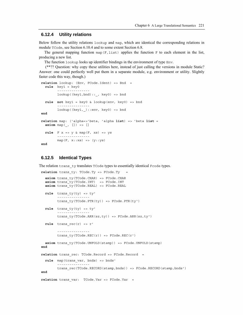
Chapter 6 A Large Translational Semantics 221
6.12.4 Utility relations
Below follow the utility relations lookup and map, which are identical the corresponding relations in module TCode, see Section 6.10.4 and to some extent Section 6.8.
The general mapping function map(F,list) applies the function F to each element in the list, producing a new list.
The function lookup looks up identifier bindings in the environment of type Env. (**?? Question: why copy these utilities here, instead of just calling the versions in module Static?
Answer: one could perfectly well put them in a separate module, e.g. environment or utility. Slightly faster code this way, though.) relation lookup: (Env, FCode.Ident) => Bnd = rule key1 = key0 ---------------- lookup((key1,bnd)::_, key0) => bnd rule not key1 = key0 & lookup(env, key0) => bnd ---------------- lookup((key1,_)::env, key0) => bnd end relation map: (’alpha=>’beta, ’alpha list) => ’beta list = axiom map(_, []) => [] rule F x => y & map(F, xs) => ys ---------------- map(F, x::xs) => (y::ys) end
6.12.5 Identical Types
The relation trans_ty translates TCode types to essentially identical Fcode types. relation trans_ty: TCode.Ty => FCode.Ty =
axiom trans_ty(TCode.CHAR) => FCode.CHAR axiom trans_ty(TCode.INT) => FCode.INT axiom trans_ty(TCode.REAL) => FCode.REAL rule trans_ty(ty) => ty' ---------------- trans_ty(TCode.PTR(ty)) => FCode.PTR(ty') rule trans_ty(ty) => ty' ---------------- trans_ty(TCode.ARR(sz,ty)) => FCode.ARR(sz,ty') rule trans_rec(r) => r' ---------------- trans_ty(TCode.REC(r)) => FCode.REC(r') axiom trans_ty(TCode.UNFOLD(stamp)) => FCode.UNFOLD(stamp) end relation trans_rec: TCode.Record => FCode.Record =
rule map(trans_var, bnds) => bnds' ---------------- trans_rec(TCode.RECORD(stamp,bnds)) => FCode.RECORD(stamp,bnds') end relation trans_var: TCode.Var => FCode.Var =

222 Peter Fritzson Generation of Language Implementations from Structural and Natural Semantics
rule trans_ty(ty) => ty' ---------------- trans_var(TCode.VAR(id,ty)) => FCode.VAR(id,ty') end relation trans_tyopt: TCode.Ty option => FCode.Ty option = axiom trans_tyopt NONE => NONE rule trans_ty(ty) => ty' ---------------- trans_tyopt(SOME(ty)) => SOME(ty') end
6.12.6 Identical Operators
The relations trans_unop and trans_binop translate TCode operators to essentially identical FCode counterparts. relation trans_unop: TCode.UnOp => FCode.UnOp =
axiom trans_unop(TCode.CtoI) => FCode.CtoI axiom trans_unop(TCode.ItoR) => FCode.ItoR axiom trans_unop(TCode.RtoI) => FCode.RtoI axiom trans_unop(TCode.ItoC) => FCode.ItoC axiom trans_unop(TCode.PtoI) => FCode.PtoI rule trans_ty(ty) => ty' ---------------- trans_unop(TCode.TOPTR(ty)) => FCode.TOPTR(ty') rule trans_ty(ty) => ty' ---------------- trans_unop(TCode.LOAD(ty)) => FCode.LOAD(ty') rule trans_rec(r) => r' ---------------- trans_unop(TCode.OFFSET(r,id)) => FCode.OFFSET(r',id) end relation trans_binop: TCode.BinOp => FCode.BinOp = axiom trans_binop(TCode.IADD) => FCode.IADD axiom trans_binop(TCode.ISUB) => FCode.ISUB axiom trans_binop(TCode.IMUL) => FCode.IMUL axiom trans_binop(TCode.IDIV) => FCode.IDIV axiom trans_binop(TCode.IMOD) => FCode.IMOD axiom trans_binop(TCode.IAND) => FCode.IAND axiom trans_binop(TCode.IOR) => FCode.IOR axiom trans_binop(TCode.ILT) => FCode.ILT axiom trans_binop(TCode.ILE) => FCode.ILE axiom trans_binop(TCode.IEQ) => FCode.IEQ axiom trans_binop(TCode.RADD) => FCode.RADD axiom trans_binop(TCode.RSUB) => FCode.RSUB axiom trans_binop(TCode.RMUL) => FCode.RMUL axiom trans_binop(TCode.RDIV) => FCode.RDIV axiom trans_binop(TCode.RLT) => FCode.RLT axiom trans_binop(TCode.RLE) => FCode.RLE axiom trans_binop(TCode.REQ) => FCode.REQ rule trans_ty(ty) => ty' ----------------

Chapter 6 A Large Translational Semantics 223
trans_binop(TCode.PADD(ty)) => FCode.PADD(ty') rule trans_ty(ty) => ty' ---------------- trans_binop(TCode.PSUB(ty)) => FCode.PSUB(ty') rule trans_ty(ty) => ty' ---------------- trans_binop(TCode.PDIFF(ty)) => FCode.PDIFF(ty') rule trans_ty(ty) => ty' ---------------- trans_binop(TCode.PLT(ty)) => FCode.PLT(ty') rule trans_ty(ty) => ty' ---------------- trans_binop(TCode.PLE(ty)) => FCode.PLE(ty') rule trans_ty(ty) => ty' ---------------- trans_binop(TCode.PEQ(ty)) => FCode.PEQ(ty') end
The relation trans_procid retrieves the translated (unambiguous) procedure name from the work environment used during flattening. For example, for a procedure foo declared within a procedure fie, it would retrieve the name fie_foo, i.e., the enclosing names are used as a prefix. relation trans_procid: (Env, TCode.Ident) => FCode.Ident = rule lookup(env, id) => PROC id' ---------------- trans_procid(env, id) => id' end
6.12.7 Expressions
The relation trans_exp translates TCode expressions to FCode expressions. Everything is identical in the FCode, except variable references and procedure/function calls.
In the rule for variable references, variable accesses are translated to an expression (in C syntax, approximately (struct r*)DISPLAY[lev]->id) that can handle accesses to intermediate-level non-local variables, as well as local variables, via display or static links.
In the rule for procedure names, the relation trans_procid translates a procedure name to a disambiguated name, as already mentioned a few times. relation trans_exp: (Env, TCode.Exp) => FCode.Exp =
axiom trans_exp(_, TCode.ICON(x)) => FCode.ICON(x) axiom trans_exp(_, TCode.RCON(x)) => FCode.RCON(x) (* Lookup a variable id at scope level lev, in activation recordtype r * C syntax version: (struct r* )DISPLAY[lev]->id *) rule lookup(env, id) => VAR(lev,r) ---------------- trans_exp(env, TCode.ADDR(id)) => FCode.UNARY(FCode.OFFSET(r,id), FCode.UNARY(FCode.TOPTR(FCode.REC(r)), FCode.DISPLAY(lev))) rule trans_unop unop => unop’ & trans_exp(env, exp) => exp’ ---------------- trans_exp(env, TCode.UNARY(unop,exp)) => FCode.UNARY(unop’,exp’) rule trans_binop binop => binop’ &

224 Peter Fritzson Generation of Language Implementations from Structural and Natural Semantics
trans_exp(env, exp1) => exp1’ & trans_exp(env, exp2) => exp2’ ---------------- trans_exp(env, TCode.BINARY(exp1,binop,exp2)) => FCode.BINARY(exp1’,binop’,exp2’) (* Translate the Tcode procedure name to the disambiguated Fcode name *) rule trans_procid(env, id) => id’ & trans_args(env, args, []) => args’ ---------------- trans_exp(env, TCode.FCALL(id,args)) => FCode.FCALL(id’,args’) end relation trans_args: (Env, TCode.Exp list, FCode.Exp list) => FCode.Exp list = rule list_reverse(args') => args'' ---------------- trans_args(_, [], args') => args'' rule trans_exp(env, arg) => arg' & trans_args(env, args, arg'::args') => args'' ---------------- trans_args(env, arg::args, args') => args'' end
Just translate a procedure/function return to the same in FCode. relation trans_return: (Env, (TCode.Ty * TCode.Exp) option) => (FCode.Ty * FCode.Exp) option =
axiom trans_return(_, NONE) => NONE rule trans_ty(ty) => ty' & trans_exp(env, exp) => exp' ---------------- trans_return(env, SOME((ty,exp))) => SOME((ty',exp')) end
6.12.8 Statements
The relation trans_stmt translates TCode statement representation to FCode. Everything is identical, except procedure call statements where the procedure name of nested procedures is changed. Also, of course, variable references within embedded expressions are also changed. relation trans_stmt: (Env, TCode.Stmt) => FCode.Stmt =
rule trans_ty(ty) => ty’ & trans_exp(env, lhs) => lhs’ & trans_exp(env, rhs) => rhs’ ---------------- trans_stmt(env, TCode.STORE(ty,lhs,rhs)) => FCode.STORE(ty’,lhs’,rhs’) (* Translate procedure identifier *) rule trans_procid(env, id) => id’ & trans_args(env, args, []) => args’ ---------------- trans_stmt(env, TCode.PCALL(id,args)) => FCode.PCALL(id’,args’) rule trans_return(env, ret) => ret’ ---------------- trans_stmt(env, TCode.RETURN(ret)) => FCode.RETURN(ret’) rule trans_exp(env, exp) => exp’ & trans_stmt(env, stmt) => stmt’ ---------------- trans_stmt(env, TCode.WHILE(exp,stmt)) => FCode.WHILE(exp’,stmt’)

Chapter 6 A Large Translational Semantics 225
rule trans_exp(env, exp) => exp’ & trans_stmt(env, stmt1) => stmt1’ & trans_stmt(env, stmt2) => stmt2’ ---------------- trans_stmt(env,TCode.IF(exp,stmt1,stmt2)) => FCode.IF(exp’,stmt1’,stmt2’) rule trans_stmt(env, stmt1) => stmt1’ & trans_stmt(env, stmt2) => stmt2’ ---------------- trans_stmt(env, TCode.SEQ(stmt1,stmt2)) => FCode.SEQ(stmt1’,stmt2’) axiom trans_stmt(_, TCode.SKIP) => FCode.SKIP end
6.12.9 Procedures, Functions and Programs
The relations flatten_proc and flatten flattens procedures/functions and whole programs, respectively, as already described in Section 6.12.1. The called relations env_plus_vars and flatten_procs are defined below, whereas trans_stmt is defined in the previous section and trans_tyopt is defined in Section 6.12.5. relation flatten_proc: (Scope, Env, TCode.Proc, FCode.Proc list) => (Env, FCode.Proc list) = (* External procedures without body *) rule map(trans_var, formals) => formals’ & trans_tyopt tyopt => tyopt’ ---------------- flatten_proc(_, env0, TCode.PROC(id,formals,tyopt,NONE), procs0) => ((id,PROC id)::env0, FCode.PROC(id,formals’,tyopt’,NONE)::procs0) (* Module internal procedures with a body *) rule int_add(level0, 1) => level1 & string_append(prefix0, id) => id’ & string_append(id’, "_") => prefix1 & map(trans_var, formals) => formals’ & map(trans_var, locals) => locals’ & list_append(formals’, locals’) => vars’ & tick => stamp & let r = FCode.RECORD(stamp,vars’) & let env1 = (id,PROC id’)::env0 & env_plus_vars(env1, VAR(level1,r), vars’) => env2 & flatten_procs(SCOPE(level1,prefix1), env2, procs, procs0) => (env3,procs1) & trans_stmt(env3, stmt) => stmt’ & trans_tyopt tyopt => tyopt’ ---------------- flatten_proc( SCOPE(level0,prefix0), env0, TCode.PROC(id,formals,tyopt, SOME(TCode.BLOCK(locals,procs,stmt))), procs0) => ( env1, FCode.PROC(id’, formals’, tyopt’, SOME(FCode.BLOCK(level1,r,stmt’)))::procs1 ) end
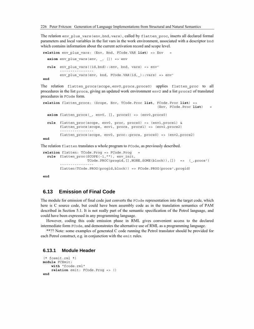
226 Peter Fritzson Generation of Language Implementations from Structural and Natural Semantics
The relation env_plus_vars(env,bnd,vars), called by flatten_proc, inserts all declared formal parameters and local variables in the list vars in the work environment, associated with a descriptor bnd which contains information about the current activation record and scope level. relation env_plus_vars: (Env, Bnd, FCode.VAR list) => Env =
axiom env_plus_vars(env, _, []) => env rule env_plus_vars((id,bnd)::env, bnd, vars) => env' ---------------- env_plus_vars(env, bnd, FCode.VAR(id,_)::vars) => env' end
The relation flatten_procs(scope,env0,procs,procs0) applies flatten_proc to all procedures in the list procs, giving an updated work environment env2 and a list procs2 of translated procedures in FCode form. relation flatten_procs: (Scope, Env, TCode.Proc list, FCode.Proc list) => (Env, FCode.Proc list) = axiom flatten_procs(_, env0, [], procs0) => (env0,procs0) rule flatten_proc(scope, env0, proc, procs0) => (env1,procs1) & flatten_procs(scope, env1, procs, procs1) => (env2,procs2) ---------------- flatten_procs(scope, env0, proc::procs, procs0) => (env2,procs2) end
The relation flatten translates a whole program to FCode, as previously described. relation flatten: TCode.Prog => FCode.Prog = rule flatten_proc(SCOPE(-1,""), env_init, TCode.PROC(progid,[],NONE,SOME(block)),[]) => (_,procs') ---------------- flatten(TCode.PROG(progid,block)) => FCode.PROG(procs',progid) end
6.13 Emission of Final Code The module for emission of final code just converts the FCode representation into the target code, which here is C source code, but could have been assembly code as in the translation semantics of PAM described in Section 5.1. It is not really part of the semantic specification of the Petrol language, and could have been expressed in any programming language.
However, coding this code emission phase in RML gives convenient access to the declared intermediate form FCode, and demonstrates the alternative use of RML as a programming language.
**?? Note: some examples of generated C code running the Petrol translator should be provided for each Petrol construct, e.g. in conjunction with the emit rules.
6.13.1 Module Header (* fcemit.rml *) module FCEmit: with "fcode.rml" relation emit: FCode.Prog => () end

Chapter 6 A Large Translational Semantics 227
6.13.2 Utility Procedures relation foreach: (’alpha=>(), ’alpha list) => () = axiom foreach(_, []) rule F x & foreach(F, xs) ---------------- foreach(F, x::xs) end relation map: (’alpha=>’beta, ’alpha list) => ’beta list = axiom map(_, []) => [] rule F x => y & map(F, xs) => ys ---------------- map(F, x::xs) => (y::ys) end
6.13.3 Data Structures
The following data structures are needed when converting the prefix type representation of FCode to the postfix (inverted) type representation needed when emitting C code. datatype Base = BASE of string | REC of int datatype InvTy = PTRity of InvTy | ARRity of InvTy * int | VARity of string | FUNity of string * Arg list and Arg = ARG of Base * InvTy
6.13.4 Emitting (Inverted) C Types relation emit_int: int => () = rule int_string(i) => s & print s --------- emit_int(i) end relation emit_real: real => () = rule real_string r => s & print s --------- emit_real(r) end relation emit_struct: int => () = rule print "struct rec" & emit_int(stamp) ---------------- emit_struct(stamp) end relation emit_base: Base => () = rule print str ----------------

228 Peter Fritzson Generation of Language Implementations from Structural and Natural Semantics
emit_base(BASE str) rule emit_struct(stamp) ---------------- emit_base(REC(stamp)) end relation emit_invty: InvTy => () = rule print "(" & print "*" & emit_invty(ity) & print ")" ---------------- emit_invty(PTRity(ity)) rule emit_invty(ity) & print "[" & emit_int(sz) & print "]" ---------------- emit_invty(ARRity(ity,sz)) rule print str ---------------- emit_invty(VARity(str)) rule print id & print "(" & emit_args(args) & print ")" ---------------- emit_invty(FUNity(id,args)) end relation emit_args: Arg list => () = rule print "void" ---------------- emit_args([]) rule emit_arg(arg) & foreach(emit_comma_arg, args) ---------------- emit_args(arg::args) end relation emit_arg: Arg => () = rule emit_base(base) & print " " & emit_invty(ity) ---------------- emit_arg(ARG(base, ity)) end relation emit_comma_arg: Arg => () = rule print ", " & emit_arg arg ---------------- emit_comma_arg arg end relation invert_ty: (InvTy, FCode.Ty) => (Base, InvTy) = (** Invert type representation (Prefix form) to C form (see thesis) *) axiom invert_ty(ity, FCode.CHAR) => (BASE "char", ity) axiom invert_ty(ity, FCode.INT) => (BASE "int", ity) axiom invert_ty(ity, FCode.REAL) => (BASE "double", ity) rule invert_ty(PTRity(ity), ty) => (base, ity’) ---------------- invert_ty(ity, FCode.PTR(ty)) => (base, ity’) rule invert_ty(ARRity(ity,sz), ty) => (base, ity’) ---------------- invert_ty(ity, FCode.ARR(sz,ty)) => (base, ity’) axiom invert_ty(ity, FCode.REC(FCode.RECORD(stamp,_))) => (REC(stamp), ity)
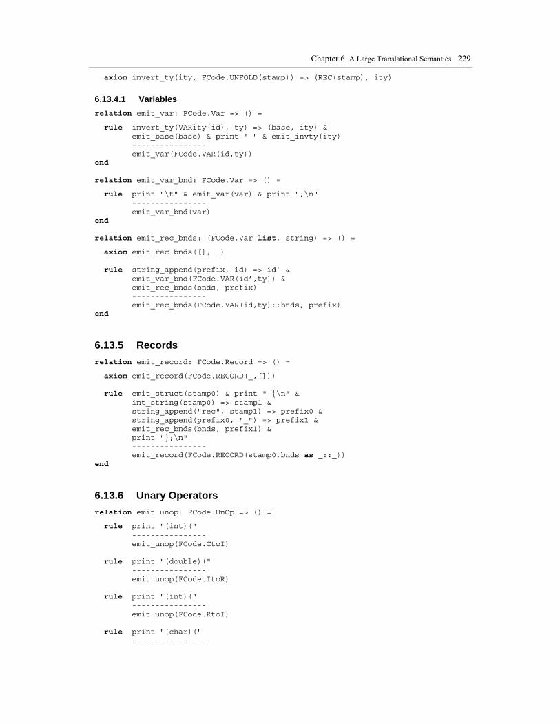
Chapter 6 A Large Translational Semantics 229
axiom invert_ty(ity, FCode.UNFOLD(stamp)) => (REC(stamp), ity)
6.13.4.1 Variables relation emit_var: FCode.Var => () =
rule invert_ty(VARity(id), ty) => (base, ity) & emit_base(base) & print " " & emit_invty(ity) ---------------- emit_var(FCode.VAR(id,ty)) end relation emit_var_bnd: FCode.Var => () =
rule print "\t" & emit_var(var) & print ";\n" ---------------- emit_var_bnd(var) end relation emit_rec_bnds: (FCode.Var list, string) => () =
axiom emit_rec_bnds([], _) rule string_append(prefix, id) => id’ & emit_var_bnd(FCode.VAR(id’,ty)) & emit_rec_bnds(bnds, prefix) ---------------- emit_rec_bnds(FCode.VAR(id,ty)::bnds, prefix) end
6.13.5 Records relation emit_record: FCode.Record => () =
axiom emit_record(FCode.RECORD(_,[])) rule emit_struct(stamp0) & print " {\n" & int_string(stamp0) => stamp1 & string_append("rec", stamp1) => prefix0 & string_append(prefix0, "_") => prefix1 & emit_rec_bnds(bnds, prefix1) & print "};\n" ---------------- emit_record(FCode.RECORD(stamp0,bnds as _::_)) end
6.13.6 Unary Operators relation emit_unop: FCode.UnOp => () =
rule print "(int)(" ---------------- emit_unop(FCode.CtoI) rule print "(double)(" ---------------- emit_unop(FCode.ItoR) rule print "(int)(" ---------------- emit_unop(FCode.RtoI) rule print "(char)(" ----------------

230 Peter Fritzson Generation of Language Implementations from Structural and Natural Semantics
emit_unop(FCode.ItoC) rule print "(int)(" ---------------- emit_unop(FCode.PtoI) rule print "(" & invert_ty(VARity(""), FCode.PTR(ty)) => (base, ity) & emit_base(base) & print " " & emit_invty(ity) & print ")(" ---------------- emit_unop(FCode.TOPTR(ty)) rule print "*(" ---------------- emit_unop(FCode.LOAD(_)) rule print "P_OFFSET(rec" & emit_int(stamp) & print "_" & print id & print "," ---------------- emit_unop(FCode.OFFSET(FCode.RECORD(stamp,_),id)) end
6.13.7 Binary Operators relation binop_to_str: FCode.BinOp => string = axiom binop_to_str(FCode.IADD) => " + " axiom binop_to_str(FCode.ISUB) => " - " axiom binop_to_str(FCode.IMUL) => " * " axiom binop_to_str(FCode.IDIV) => " / " axiom binop_to_str(FCode.IMOD) => " % " axiom binop_to_str(FCode.IAND) => " && " axiom binop_to_str(FCode.IOR) => " || " axiom binop_to_str(FCode.ILT) => " < " axiom binop_to_str(FCode.ILE) => " <= " axiom binop_to_str(FCode.IEQ) => " == " axiom binop_to_str(FCode.RADD) => " + " axiom binop_to_str(FCode.RSUB) => " - " axiom binop_to_str(FCode.RMUL) => " * " axiom binop_to_str(FCode.RDIV) => " / " axiom binop_to_str(FCode.RLT) => " < " axiom binop_to_str(FCode.RLE) => " <= " axiom binop_to_str(FCode.REQ) => " == " axiom binop_to_str(FCode.PADD(_)) => " + " axiom binop_to_str(FCode.PSUB(_)) => " - " axiom binop_to_str(FCode.PDIFF(_)) => " - " axiom binop_to_str(FCode.PLT(_)) => " < " axiom binop_to_str(FCode.PLE(_)) => " <= " axiom binop_to_str(FCode.PEQ(_)) => " == " end
6.13.8 Expressions relation emit_exp: FCode.Exp => () =
rule emit_int(i) ---------------- emit_exp(FCode.ICON(i))

Chapter 6 A Large Translational Semantics 231
rule emit_real(r) ---------------- emit_exp(FCode.RCON(r)) rule print "display[" & emit_int(level) & print "]" ---------------- emit_exp(FCode.DISPLAY(level)) rule emit_unop(unop) & emit_exp(exp) & print ")" ---------------- emit_exp(FCode.UNARY(unop, exp)) rule print "((" & emit_exp(exp1) & print ")" & binop_to_str(binop) => str & print str & print "(" & emit_exp(exp2) & print "))" ---------------- emit_exp(FCode.BINARY(exp1, binop, exp2)) rule print id & print "(" & emit_exps exps & print ")" ---------------- emit_exp(FCode.FCALL(id, exps)) end relation emit_comma_exp: FCode.Exp => () = rule print ", " & emit_exp(exp) ---------------- emit_comma_exp exp end relation emit_exps: FCode.Exp list => () = axiom emit_exps [] rule emit_exp(exp) & foreach(emit_comma_exp, exps) ---------------- emit_exps(exp::exps) end relation emit_assign_retval: (FCode.Ty * FCode.Exp) option => () = axiom emit_assign_retval(NONE) rule print "\tretval = " & emit_exp(exp) & print ";\n" ---------------- emit_assign_retval(SOME((_,exp))) end
6.13.9 Statements relation emit_stmt: FCode.Stmt => () =
rule print "\t*" & emit_exp(lhs) & print " = " & emit_exp(rhs) & print ";\n" ---------------- emit_stmt(FCode.STORE(_,lhs,rhs)) rule print "\t" & print id & print "(" & emit_exps exps & print ");\n" ---------------- emit_stmt(FCode.PCALL(id,exps)) rule emit_assign_retval ret & print "\tgoto epilogue;\n" ---------------- emit_stmt(FCode.RETURN(ret)) rule print "\twhile( " & emit_exp(exp) & print " ) {\n" & emit_stmt stmt & print "\t}\n"

232 Peter Fritzson Generation of Language Implementations from Structural and Natural Semantics
---------------- emit_stmt(FCode.WHILE(exp,stmt)) rule print "\tif( " & emit_exp(exp) & print " ) {\n" & emit_stmt stmt1 & print "\t} else {\n" & emit_stmt stmt2 & print "\t}\n" ---------------- emit_stmt(FCode.IF(exp,stmt1,stmt2)) rule emit_stmt stmt1 & emit_stmt stmt2 ---------------- emit_stmt(FCode.SEQ(stmt1,stmt2)) axiom emit_stmt(FCode.SKIP) end relation conv_formal_decl: FCode.Var => Arg = rule invert_ty(VARity(""), ty) => (base,ity) ---------------- conv_formal_decl(FCode.VAR(_,ty)) => ARG(base,ity) end relation emit_proc_head: (FCode.Ty option, FCode.Ident, Arg list) => () = rule print "void " & print id & print "(" & emit_args(args) & print ")" ---------------- emit_proc_head(NONE, id, args) rule invert_ty(FUNity(id,args), ty) => (base, ity) & emit_base(base) & print " " & emit_invty(ity) ---------------- emit_proc_head(SOME(ty), id, args) end relation emit_proc_decl: FCode.Proc => () = rule map(conv_formal_decl, formals) => formals’ & print "extern " & emit_proc_head(ty_opt, id, formals’) & print ";\n" ---------------- emit_proc_decl(FCode.PROC(id,formals,ty_opt,_)) end relation conv_formal_defn: FCode.Var => Arg = rule invert_ty(VARity(id), ty) => (base, ity) ---------------- conv_formal_defn(FCode.VAR(id,ty)) => ARG(base,ity) end relation emit_decl_retval: FCode.Ty option => () = axiom emit_decl_retval(NONE) rule emit_var_bnd(FCode.VAR("retval",ty)) ---------------- emit_decl_retval(SOME(ty)) end relation emit_return_retval: FCode.Ty option => () = axiom emit_return_retval(NONE) rule print "\treturn retval;\n" ---------------- emit_return_retval(SOME(_)) end relation emit_load_formals: (FCode.Var list, string) => () = axiom emit_load_formals([], _)

Chapter 6 A Large Translational Semantics 233
rule print "\tframe.rec" & print stamp & print "_" & print id & print " = " & print id & print ";\n" & emit_load_formals(formals, stamp) ---------------- emit_load_formals(FCode.VAR(id,_)::formals, stamp) end
6.13.10 Display Handling
Note: Procedures may have empty activation records, represented as empty record types. However, C does not allow empty struct types, which is the reason the axiom does not emit any C code. relation emit_setup_display: (FCode.Level, FCode.Var list, FCode.Record) => () =
axiom emit_setup_display(_, _, FCode.RECORD(_,[])) rule print "\t" & emit_struct(stamp) & print " frame;\n" & print "\tvoid *saveFP = display[" & emit_int(lev) & print "];\n" & print "\tdisplay[" & emit_int(lev) & print "] = &frame;\n" & int_string(stamp) => stamp’ & emit_load_formals(formals, stamp’) ---------------- emit_setup_display(lev, formals, FCode.RECORD(stamp,vars as _::_)) end relation emit_restore_display: (FCode.Level, FCode.Record) => () = axiom emit_restore_display(_, FCode.RECORD(_,[])) rule print "\tdisplay[" & emit_int(lev) & print "] = saveFP;\n" ---------------- emit_restore_display(lev, FCode.RECORD(_,_::_)) end
6.13.11 Emit Procedure relation emit_proc_defn: FCode.Proc => () =
axiom emit_proc_defn(FCode.PROC(_,_,_,NONE)) rule map(conv_formal_defn, formals) => formals’ & emit_proc_head(ty_opt, id, formals’) & print "\n{\n" & emit_decl_retval ty_opt & emit_setup_display(lev,formals,r) & emit_stmt stmt & print "epilogue:;\n" & emit_restore_display(lev,r) & emit_return_retval ty_opt & print "}\n" ---------------- emit_proc_defn(FCode.PROC(id,formals,ty_opt, SOME(FCode.BLOCK(lev,r,stmt)))) end
6.13.12 Extract and Emit all Used Record Types (* * RECORDS, for binary search tree storing record types. *) datatype Cmp = LT | EQ | GT
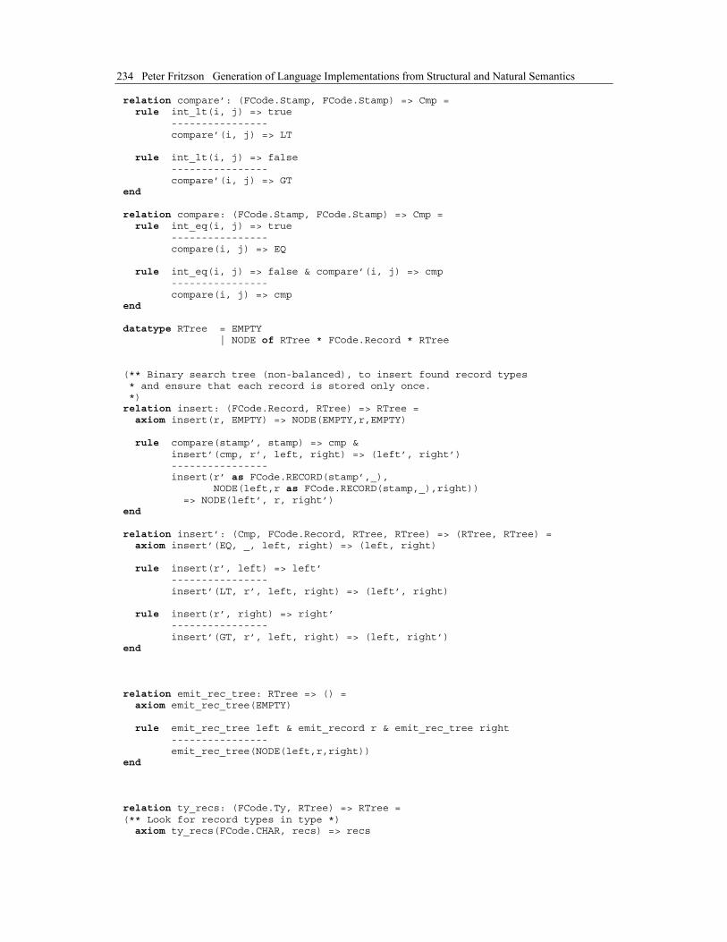
234 Peter Fritzson Generation of Language Implementations from Structural and Natural Semantics
relation compare’: (FCode.Stamp, FCode.Stamp) => Cmp = rule int_lt(i, j) => true ---------------- compare’(i, j) => LT rule int_lt(i, j) => false ---------------- compare’(i, j) => GT end relation compare: (FCode.Stamp, FCode.Stamp) => Cmp = rule int_eq(i, j) => true ---------------- compare(i, j) => EQ rule int_eq(i, j) => false & compare’(i, j) => cmp ---------------- compare(i, j) => cmp end datatype RTree = EMPTY | NODE of RTree * FCode.Record * RTree (** Binary search tree (non-balanced), to insert found record types * and ensure that each record is stored only once. *) relation insert: (FCode.Record, RTree) => RTree = axiom insert(r, EMPTY) => NODE(EMPTY,r,EMPTY) rule compare(stamp’, stamp) => cmp & insert’(cmp, r’, left, right) => (left’, right’) ---------------- insert(r’ as FCode.RECORD(stamp’,_), NODE(left,r as FCode.RECORD(stamp,_),right)) => NODE(left’, r, right’) end relation insert’: (Cmp, FCode.Record, RTree, RTree) => (RTree, RTree) = axiom insert’(EQ, _, left, right) => (left, right) rule insert(r’, left) => left’ ---------------- insert’(LT, r’, left, right) => (left’, right) rule insert(r’, right) => right’ ---------------- insert’(GT, r’, left, right) => (left, right’) end relation emit_rec_tree: RTree => () = axiom emit_rec_tree(EMPTY) rule emit_rec_tree left & emit_record r & emit_rec_tree right ---------------- emit_rec_tree(NODE(left,r,right)) end relation ty_recs: (FCode.Ty, RTree) => RTree = (** Look for record types in type *) axiom ty_recs(FCode.CHAR, recs) => recs

Chapter 6 A Large Translational Semantics 235
axiom ty_recs(FCode.INT, recs) => recs axiom ty_recs(FCode.REAL, recs) => recs rule ty_recs(ty, recs0) => recs1 ---------------- ty_recs(FCode.PTR(ty), recs0) => recs1 rule ty_recs(ty, recs0) => recs1 ---------------- ty_recs(FCode.ARR(_,ty), recs0) => recs1 (** Insert the found record r into recs0 *) rule insert(r, recs0) => recs1 & vars_recs(bnds, recs1) => recs2 ---------------- ty_recs(FCode.REC(r as FCode.RECORD(_,bnds)), recs0) => recs2 axiom ty_recs(FCode.UNFOLD(_), recs) => recs end relation vars_recs: (FCode.Var list, RTree) => RTree = axiom vars_recs([], recs) => recs rule ty_recs(ty, recs0) => recs1 & vars_recs(vars, recs1) => recs2 ---------------- vars_recs(FCode.VAR(_,ty)::vars, recs0) => recs2 end relation ty_opt_recs: (FCode.Ty option, RTree) => RTree = axiom ty_opt_recs(NONE, recs) => recs rule ty_recs(ty, recs0) => recs1 ---------------- ty_opt_recs(SOME(ty), recs0) => recs1 end relation unop_recs: (FCode.UnOp, RTree) => RTree = rule ty_recs(ty, recs0) => recs1 ---------------- unop_recs(FCode.TOPTR(ty), recs0) => recs1 axiom unop_recs(FCode.CtoI, recs) => recs axiom unop_recs(FCode.ItoR, recs) => recs axiom unop_recs(FCode.RtoI, recs) => recs axiom unop_recs(FCode.ItoC, recs) => recs axiom unop_recs(FCode.PtoI, recs) => recs axiom unop_recs(FCode.LOAD(_), recs) => recs axiom unop_recs(FCode.OFFSET(_,_), recs) => recs end relation exp_recs: (FCode.Exp, RTree) => RTree = axiom exp_recs(FCode.ICON(_), recs) => recs axiom exp_recs(FCode.RCON(_), recs) => recs axiom exp_recs(FCode.DISPLAY(_), recs) => recs (** A unary operator PTR may refer to a record type from unop_recs *) rule unop_recs(unop, recs0) => recs1 & exp_recs(exp, recs1) => recs2 ---------------- exp_recs(FCode.UNARY(unop,exp), recs0) => recs1

236 Peter Fritzson Generation of Language Implementations from Structural and Natural Semantics
rule exp_recs(exp1, recs0) => recs1 & exp_recs(exp2, recs1) => recs2 ---------------- exp_recs(FCode.BINARY(exp1,_,exp2), recs0) => recs2 rule exps_recs(exps, recs0) => recs1 ---------------- exp_recs(FCode.FCALL(_,exps), recs0) => recs1 end relation exps_recs: (FCode.Exp list, RTree) => RTree = axiom exps_recs([], recs) => recs rule exp_recs(exp, recs0) => recs1 & exps_recs(exps, recs1) => recs2 ---------------- exps_recs(exp::exps, recs0) => recs2 end relation stmt_recs: (FCode.Stmt, RTree) => RTree = (** Traverse all statement and expressions, to find record types * which are referenced. *) rule ty_recs(ty, recs0) => recs1 & exp_recs(exp1, recs1) => recs2 & exp_recs(exp2, recs2) => recs3 ---------------- stmt_recs(FCode.STORE(ty,exp1,exp2), recs0) => recs3 rule exps_recs(exps, recs0) => recs1 ---------------- stmt_recs(FCode.PCALL(_,exps), recs0) => recs1 axiom stmt_recs(FCode.RETURN(NONE), recs) => recs rule exp_recs(exp, recs0) => recs1 ---------------- stmt_recs(FCode.RETURN(SOME((_,exp))), recs0) => recs1 rule exp_recs(exp, recs0) => recs1 & stmt_recs(stmt, recs1) => recs2 ---------------- stmt_recs(FCode.WHILE(exp,stmt), recs0) => recs2 rule exp_recs(exp, recs0) => recs1 & stmt_recs(stmt1, recs1) => recs2 & stmt_recs(stmt2, recs2) => recs3 ---------------- stmt_recs(FCode.IF(exp,stmt1,stmt2), recs0) => recs3 rule stmt_recs(stmt1, recs0) => recs1 & stmt_recs(stmt2, recs1) => recs2 ---------------- stmt_recs(FCode.SEQ(stmt1,stmt2), recs0) => recs2 axiom stmt_recs(FCode.SKIP, recs) => recs end relation block_opt_recs: (FCode.Block option, RTree) => RTree = (** Insert activation record r in the set recs0 of activation records, * , giving recs2 *) axiom block_opt_recs(NONE, recs) => recs

Chapter 6 A Large Translational Semantics 237
(** Insert found record type r *) rule insert(r, recs0) => recs1 & stmt_recs(stmt, recs1) => recs2 ---------------- block_opt_recs(SOME(FCode.BLOCK(_,r,stmt)), recs0) => recs2 end relation proc_recs: (FCode.Proc, RTree) => RTree = (** Extract possible records from formals, etc. * In all places where there might be types. * Record types for procedure parameters must be generated, since * C procedures are called from elsewhere. * Local variables are only visible inside the procedure, and * are declared in the activation record. *) rule vars_recs(formals, recs0) => recs1 & ty_opt_recs(ty_opt, recs1) => recs2 & block_opt_recs(block_opt, recs2) => recs3 ---------------- proc_recs(FCode.PROC(_,formals,ty_opt,block_opt), recs0) => recs3 end relation procs_recs: (FCode.Proc list, RTree) => RTree = axiom procs_recs([], recs) => recs rule proc_recs(proc, recs0) => recs1 & procs_recs(procs, recs1) => recs2 ---------------- procs_recs(proc::procs, recs0) => recs2 end (** Traverse all procedures, and create a set of all records which are * used (recs), and emit declarations for these records. *) relation emit_record_defns: FCode.Proc list => () = rule procs_recs(procs, EMPTY) => recs & emit_rec_tree recs ---------------- emit_record_defns procs end
6.13.13 Emit a Whole Program (* * PROGRAMS *) (** Traverse all procedure declarations and print out a C struct for * each activation record *) relation emit: FCode.Proc => () = rule print "#include \"petrol.h\"\nvoid *display[16];\n" & emit_record_defns procs & foreach(emit_proc_decl, procs) & foreach(emit_proc_defn, procs) & print "int main(void)\n{\n\t" & print id & print "();\n\treturn 0;\n}\n" ---------------- emit(FCode.PROG(procs,id)) end

238 Peter Fritzson Generation of Language Implementations from Structural and Natural Semantics
6.14 Building and Running the Petrol Translator ?? fill in
6.14.1 Running the Petrol Translator
The executable is called petrol, and is invoked by typing petrol at the Unix prompt. The filename of the petrol source file that is to be compiled should be passed as a command line argument to the executable. The result is a C program printed out on the prompt. A C compiler has then to be invoked to compile this program. Input typed by the user is shown in boldface. sen4%42 petrol factorial.p > factorial.c sen4%43 cc factorial.c -o factorial sen4%44 factorial 5 120 sen4%45
6.14.2 Building the Petrol Translator
The following files are needed for building the Petrol translator: absyn.rml, fcemit.rml, fcode.rml, flatten.rml, lexer.h, lexer.c, main.rml, parse.rml, parser.y, parsutil.h, parsutil.c, petrol.h, static.rml, tcode.rml, types.rml, yacclib.h, yacclib.c and Makefile.
The files can be copied from (??changed) /home/pelab/pub/pkg/rml/current/
bookexamples/examples/petrol2. A number of test programs are available in the subdirectories testd an testp. The executable is built by typing a make command: sen4%2 make petrol
6.14.2.1 Makefile include ../../config.cache # # Makefile for the petrol example # GOROOT=../.. ETCDIR=../etc CPPFLAGS=-DLEXDEBUG=1 -DYYDEBUG=1 -I$(ETCDIR) SRCRML= absyn.rml fcemit.rml fcode.rml flatten.rml main.rml static.rml tcode.rml types.rml SRCC= $(SRCRML:.rml=.c) SRCH= $(SRCRML:.rml=.h) SRCO= $(SRCRML:.rml=.o) EXTRAO= lexer.o parser.o parsutil.o yacclib.o EXTRAC= parser.c parser.h y.tab.c y.tab.h EXTRARM=y.output ccall1.o ccall2.o BINARIES=petrol benchexe petrol.exe benchexe.exe CLEAN= $(SRCO) $(EXTRAO) $(EXTRARM) $(BINARIES) ccall.c=$(ETCDIR)/ccall.c yacclib.h=$(ETCDIR)/yacclib.h yacclib.c=$(ETCDIR)/yacclib.c ALMOSTPETROL= $(SRCO) $(EXTRAO) # default target petrol: $(ALMOSTPETROL) ccall1.o

Chapter 6 A Large Translational Semantics 239
$(LINK.rml) -o petrol $(ALMOSTPETROL) ccall1.o benchexe: $(ALMOSTPETROL) ccall2.o $(LINK.rml) -o benchexe $(ALMOSTPETROL) ccall2.o benchrun: benchexe $(RUN) ./benchexe -bench testd/big.d benchrun10: benchexe for i in 0 1 2 3 4 5 6 7 8 9; do $(RUN) ./benchexe -bench testd/big.d; done csources: $(SRCC) $(EXTRAC) ccall1.o: $(ccall.c) $(COMPILE.rml) -UBENCH -o ccall1.o $(ccall.c) ccall2.o: $(ccall.c) $(COMPILE.rml) -DBENCH -o ccall2.o $(ccall.c) lexer.o: $(yacclib.h) parsutil.h parser.h lexer.h parser.o: parser.c $(yacclib.h) parsutil.h lexer.h parsutil.o: $(yacclib.h) absyn.h parsutil.h yacclib.o: $(yacclib.c) $(yacclib.h) $(COMPILE.rml) $(yacclib.c) y.tab.c y.tab.h: parser.y $(YACC) -d parser.y $(GOROOT)/etc/fixyacc < y.tab.c > y-tab-c mv y-tab-c y.tab.c parser.c: y.tab.c $(GOROOT)/etc/cp-if-change y.tab.c parser.c parser.h: y.tab.h $(GOROOT)/etc/cp-if-change y.tab.h parser.h clean-binaries: rm -f $(BINARIES) clean-objects: rm -f $(SRCO) $(EXTRAO) ccall1.o ccall2.o clean-csources: rm -f $(SRCC) $(SRCH) $(EXTRAC) distclean: realclean clean-configure realclean: clean-csources clean include $(GOROOT)/etc/client.mk

241
Chapter 7 Specifying Type Inference
in Mini-ML
(* ?? This will become a chapter on how to specify type inference using RML, exemplified on the Mini-ML. language example*)
lkjlkj
absyn.rml,dynamic.rml,parse.rml,main1.rml,main2.rml,scheme.rml,static.rml


243
Chapter 8 Specifying Object Oriented Languages – Java
(*?? A chapter on how to specify the usual primitives of object oriented languages, such as classes, inheritance, etc. Examples from Java *)
This chapter briefly presents one of the first full-scale Structured Operational Semantics formal specifications of Java, as well as one of the first cases of automatically generating an efficient and practically usable Java compiler from such specifications.
In this chapter we present the structure of a Java 1.2 translational semantics in RML including some excerpts from the semantics specification itself. Complex issues like dealing with define after use, and lookup of definitions in large Java class libraries are discussed. In order to handle 64-bit integers it proved necessary to extend the value domain of the RML primitive arithmetic operations. The RML system was used to generate a Java compiler implemented in C, producing byte code. The compilation times of the generated compiler are approximately the same as for the Sun javac compiler on several presented examples, and the quality of generated byte code is comparable.
8.1 Specification Structure The translational semantics is structured as a sequence of translation steps. First, the source text of the program is translated to an abstract syntax tree using an ordinary syntax specification created with lex and yacc. Then, one part of the RML-based semantics specification maps the AST into an elaborated intermediate tree form, while another part transforms this elaborated tree into a sequence of JVM[4] instructions. A final translation is that from the internal representation of these instructions to the binary .class files used by the Java interpreter. The interconnection of these translations is of course also a part of the specification. The following diagram?? illustrates how the representations of a Java program are transformed into each other by the different translation steps.
??gram.y static.rml flatten.rml machine.rml
Abstract syntax tree intermediate tree form Internal byte code representation
Java byte code
lexer.l Java source code
Java Stream of tokens
lex
yacc RML RML RML

244 Peter Fritzson Generation of Language Implementations from Structural and Natural Semantics
?? Java translator, tea, is mainly generated from a Structured Operational Semantics specification of Java in RML. Other tools, Lex and Yacc are used to generate scanner and parser, and some handwritten C code is used as well.
The generated compiler parses a list of Java source files into abstract syntax trees, performs type checking, lowering of object-oriented constructs, intermediate code generation and finally an assembly pass (jazz) to emit Java byte code.
The compiler can be divided into two main parts: a program generated from a formal specification (including the scanner and parser generated from lex and yacc), and an assembler, jazz, as is shown in picture 1 ?? below
formalspecification
jazz.class
Java
source
Java
Java Compiler
textual
form
Figure 8-1. Structure of the Java compiler, where most of the compiler is generated from a formal specification, apart from the assembler, jazz, the outputs the final byte code.
The Java source files to be compiled are input to the program generated from the formal specification which then outputs a textual intermediate form further translated by jazz. Finally the corresponding .class files are output from the system.
8.1.1 Short Overview of the Java Specification Modules
The call structure between modules generated from the formal specification is depicted in ??picture 2. Arrows represent calls made to different modules, and the names printed near the arrows tell which relation is called. Finally the different numbers show in what order the different relations are called.
Main
Parser
lexer
Static Flatten
ClassFile
Machine
emit_fileParse
yylex
trans_stmtelab_types
5
87 1
63
2
store_classelab_class
Environment
4
unit
Figure 8-2. Call structure between modules generated from the formal specification .
The main controlling entity is the Main module, which acts like the spider in the web. First it calls the parser, which uses the lexical analyser, to parse the source files. When abstract syntax trees are built for the parsed programs an iterator is used to call elab_types in Static which extracts the different classes’ members. After this the define_classes relation in Main is used to resolve inheritance between the classes, and store the class declarations in the environment by calling the relation Environment.store_class.

Chapter 8 Specifying Object Oriented Languages – Java 245
With all the gathered information stored in the environment a new pass over the code is made by another iterator, calling the elab_class relation in module static for every declared class. This time all method bodies etc are gone through, translating the abstract syntax trees to a new intermediate representation.
Next, a pass over the program is done by calling the trans_stmt relation in module Flatten, which translates the output from elab_class into a sequence of virtual machine instructions.
Finally control is passed to module Classfile, which has a relation emit_file which is called one time for every class declared in the Java program. This relation then outputs the declared class in a textual intermediate representation, using Machine.unit to output the actual method bodies.
The Environment module is also used frequently at other points, both by Main and Static. However it would render the picture unreadable to add all those calls. Also a couple of helper modules are used but they are omitted in the above picture for readability.
8.1.1.1 Module Abstract
This module provides the data structures used in the parser to build Abstract Syntax Trees, ASTs.
8.1.1.2 Module Access
The Access module provides data structures and relations for handling access modifiers (private, static etc.) throughout the specification.
8.1.1.3 Module Cast
This is a helper module for Static which handles the type conversions and promotions as specified in JLS§5.
8.1.1.4 Module ClassFile
Providing the emit_unit relation, this module is responsible for emitting the textual byte code assembly representation of the compiled Java program. First the generated constant pool is translated, then the class’ fields and methods are handled. It uses the Machine.unit relation to emit method bodies.
8.1.1.5 Module ClassLoader
This module provides relations, written in C, doing the low level parsing of precompiled .class files needed by the Environment module.
8.1.1.6 Module Constant
To be able to correctly output the constant pool described in JVMS§4.4 this module is used.
8.1.1.7 Module Environment
This module contains handling of state variables, such as lexical scope. It is also responsible for keeping the database of available classes, and loading precompiled classes when they are needed.
8.1.1.8 Module Flatten
The purpose of this module is to transform the different members specified by the Tree representation to a sequence of virtual machine instructions, defined in the Machine module.
The transformation is carried out by the relation trans_stmt which has separate rules for every member of the Tree.STMT union type.

246 Peter Fritzson Generation of Language Implementations from Structural and Natural Semantics
The result of the transformation is a sequence of instructions, and a constant pool, holding the literals used in the source code that are too large to push on the virtual machine stack using the Java Virtual Machine push instruction.
8.1.1.9 Lexical analyzer
The lexical analyzer is generated by using lex. It is used to identify the tokens in the source code and send them to the parser.
8.1.1.10 Module Machine
This module provides the unit relation which translates the generated sequence of instructions that are output from the Flatten module as the class’ method bodies into a textual byte code representation, readable by the jazz byte code assembler. Before emitting the method bodies a peep-hole optimizer relation is invoked to make simple optimizations on the code.
The unit relation also checks the stack usage of the generated code and inserts this information in the output symbolic byte code.
8.1.1.11 Module Main
The Main module is the controlling module of the compiler. First it calls the parser once for each Java input file, to build the ASTs. Then a pass is done where all class member declarations are extracted. When this information is obtained a topological sort in inheritance dependence order of all the declared classes is made. The sorting is carried out such that if a class A inherits class B, then class B is compiled before class A. The reason for this sorting is that inheritance can be implemented quite straightforwardly once the sorting is made.
Next the different classes, including their inherited members, are stored in the environment. After this another pass is carried out, compiling the actual methods defined in the classes to
intermediate code and finally to byte code.
8.1.1.12 Parser
The syntactic analyzer is produced from a BNF grammar by using the yacc LALR(1) parser generator. The generated parser calls the lexical analyzer to obtain tokens, then these tokens are used to create an Abstract Syntax Tree using the RML data structures declared in module Abstract.
8.1.1.13 Module Static
This is the large module. The Static module exports two relations, elab_types and elab_class, callable from the Main module. The first one extracts a list of the members, and their types, declared in the different classes. Once this information has been collected by the Main module, the second relation is called for each class. This time all code, such as the bodies of the defined classes and initializers are traversed as well. Type analysis is performed, names are disambiguated, references to (possibly overloaded) methods are resolved etc.
Two important relations used internally in the module are elab_stmt and elab_exp, which are responsible for translating statements and expressions respectively. For every member in the Abstract.Stmt union type there is a corresponding rule in elab_stmt, and similarly there are rules in elab_exp for all constructs in Abstract.Exp.
The result from elab_class is a list of class members, specified using the intermediate representation defined in the Tree module, that subsequently will be passed to the Flatten module.
8.1.1.14 Module Tree
This module declares the data structures that are output from the static elaboration made in module Static. In this intermediate form the types of all subexpressions are immediately available just by

Chapter 8 Specifying Object Oriented Languages – Java 247
examining the expressions root node. Also all names are disambiguated, that is, it is now known whether a name refers to a field, method etc.
8.1.1.15 Module Types
This module contains data structures and relations for handling types after type names are elaborated by module Static.
8.1.1.16 jazz
The jazz assembler is responsible for carrying out the compiler’s final pass over the Java program, thus translating a textual symbolic byte code representation with jumps and labels to the standard binary Java byte code format. It is written in C.
8.2 Previous Overview: (??to be merged with the above)
8.2.1 The Main Module: main.rml
The main module calls the parser module for each input file, collecting the ASTs. It then makes a topological sort of the classes defined in the files, and passes them on to the next module in line for compilation. The classes are sorted in such a way that if class A inherits class B, then B gets compiled before A. This allows for a straightforward specification of inheritance.
Java does not allow circular inheritance, so there exists such an ordering for each correct input program. Two passes are made for each class definition; one to extract the member declarations, and one to compile the actual methods. The reason for this is that there may be forward references and mutual dependencies among the members of the classes.
8.2.2 The Static Semantics: static.rml
This module contains the bulk of the specification. It exports two different functions to the main module. The first is to provide a list of all the members declared in the AST, and their types. Once main has collected this information from all classes, the second function is called for each class. This function will again traverse the AST, but this time all code such as methods and field initializers is processed as well. This was not possible in the first pass as the environment wasn’t fully known yet. The result is a collection of members represented in the intermediate form, that will subsequently be passed to the flatten module by main.
To reduce the size of this module somewhat (even now it is almost 2000 lines long), two helper modules are used to specify some particularly involved parts of the translation. The first of these is cast.rml, which handles the type conversions and promotions specified in Java. Java has a rather intricate type system so certain rules involved are rather complex (about 500 lines) and thus good candidates for breaking out into a module of their own.
The other helper module is environment.rml, which contains handling of environment structures, including lexical scope. It is responsible for maintaining the database of available classes and their members, and also for loading precompiled classes on demand. This module has a helper module of its own (classloader.rml, which is implemented in C) which carries out the low level parsing of binary class files.

248 Peter Fritzson Generation of Language Implementations from Structural and Natural Semantics
8.2.3 Flattening the Intermediate Form: Flatten.rml
The task of flatten is to transform the method bodies expressed in the intermediate tree format into a sequence of virtual machine instructions. As the intermediate format has been designed with this transformation in mind, it is very straightforward. The result of the transformation is a sequence of instructions and an augmented Constant Pool, which holds the literals used in the code that are too large to be emitted as immediate operands in the code.
8.2.4 Abstract Virtual Machine to Byte Code: machine.rml
This module translates the abstract virtual machine code output by the flatten module into the actual sequences of bytes used in the binary class files. It will also check how much stack the code needs, and insert this information into the byte sequence for the virtual machine.
8.2.5 Internal Representations
The three intermediate representations: abstract syntax tree, intermediate tree form, and internal bytecode representation are all declared as RML union types. The abstract syntax tree is generated by the parser and thus follows the concrete grammar closely. The intermediate tree form is a simplified version of the abstract syntax tree, which has been elaborated with types where appropriate. The internal bytecode representation on the other hand is a sequence of virtual machine instructions corresponding to the Java .class files.
The elaborated intermediate tree form contains fewer more general constructors, and more type information in the expression nodes. All information about scopes and declarations of local variables has also been removed, as this information now is contained in the environment.
8.3 Selected Parts of the Specification To give a feeling for the style of the specification we now show two small excerpts from the static module. One of this module’s two entry points is the relation elab.types, which specifies the translation to a list of members declared within a class and their types. The other is the relation elab.class which specifies the actual static analysis and translation to the intermediate tree form.
8.3.1 Relation elab.types
The relation elab.types is fairly straightforward. It will recurse through the declarations contained within the class declaration and produce a mapping from name to the intermediate type representation. The actual recursion is performed by the relation elab.local.members, which appears as follows in the classical “mathematical” notation (relation names have been slightly abbreviated to save space):
(7.1)
(7.2)
E ‘ localmembers(\Gamma ; []) : hE; []i E1 ‘ localmembers(\Gamma ; \Sigma ) : hE2; \Sigma 0i E1 ‘ localmembers(\Gamma ; StaticInit(oeS) / \Sigma ) : hE2; \Sigma 0i

Chapter 8 Specifying Object Oriented Languages – Java 249
E1 ‘ type(o/ ) : hE2; o/ 0i ^ E2 ‘ localfields(\Gamma ; o/ 0; oea; \Delta ) : hE3; \Sigma 1i ^ E3 ‘ localmembers(\Gamma ; \Sigma ) : hE4; \Sigma 2i E1 ‘ localmembers(\Gamma ; Fields(oea; o/; \Delta ) / \Sigma ) : hE4; \Sigma 1 ./ \Sigma 2i E1 ‘ type(o/ ) : hE2; o/ 0i ^ E2 ‘ methodproto(o/ 0; ffi; F) : hE3; o/r; *; aei ^ E3 ‘ localmembers(\Gamma ; \Sigma ) : hE4; \Sigma 0i E1 ‘ localmembers(E1; \Gamma ; Method(MethodHdr(oea; o/; ffi; oet); oeS) / \Sigma ) : hE4; h*; METHOD(oea; \Gamma ; o/r; ae)i / \Sigma 0i E1 ‘ paramlist(reverse(oep); F) : hE2; aei ^ E2 ‘ localmembers(\Gamma ; \Sigma ) : hE3; \Sigma 0i E1 ‘ localmembers(\Gamma ; Constructor(oea; oep; oet; oeS; oei) / \Sigma ) : hE3; hp<init>q; METHOD(oea; \Gamma ; ?; ae)i / \Sigma 0i E ‘ localfields(\Gamma ; o/; oea; []) : hE; []i E1 ‘ field(o/; ffi*) : hE2; *; o/ 0i ^ E2 ‘ localfields(\Gamma ; o/; oea; \Delta ) : hE3; \Delta 0i E1 ‘ localfields(\Gamma ; o/; oea; VarDecl(ffi*; ffii) / \Delta ) : hE3; h*; FIELD(oea; \Gamma ; o/ 0; ?)i / \Delta 0i
The following table explains the usage of variables in the above rules:
Variables used in the rules
Variable Explanation
E The static environment
\ The class being translated
A list of class member declarations
An attribute of a particular class member declaration, e.g.:
A body statement
A set of access modifiers, such as private and synchronized
A throws clause
A list of formal parameters
A constructor invocation statement
A type
A return type
\ A list of declarators f
A single declarator
An identifier
A list of formal parameter types
The identifier of a declarator
The initializer expression of a declarator
The axiom at the top is the base condition that terminates the recursion. The first of the rules deals with static initializers. These are unnamed pieces of code which can not be explicitly accessed, but which are executed by the virtual machine as it loads the class. As they don’t have names they need not be taken into account in this pass.

250 Peter Fritzson Generation of Language Implementations from Structural and Natural Semantics
The second rule handles fields. There can be multiple fields with the same type declared by a single field declaration, so the relation elab.local.fields (shown at the end) is recursive as well.
Next, methods are taken care of. The relation elab.methodproto will convert the type of each formal parameter to the type format of the intermediate representation. It can also add these to the lexical scope, but the final parameter value of false tells it not to.
The final rule of elab.local.members is for constructors. Constructors are implemented in the virtual machine as methods with the name <init> (not a legal Java identifier), and the intermediate representation also uses this scheme for convenience. The constructor is thus handled almost like a method. The relation elab.paramlist is actually an inner relation of elab.methodproto, which does not handle elaboration of the return type (not needed here as constructors do not have return types).
As an illustrative example, here is how the rule appears in the actual RML code: relation elab.local.members: (Environment.Env,Types.Type, Abstract.Decl list) => (Environment.Env, Environment.Named list) = axiom elab.local.members(e,.,[]) => (e, []) rule elab.local.members(e1, n, rest) => (e2, nl) ------------------------------------------------------- elab.local.members(e1, n, Abstract.StaticInit(.)::rest) => (e2, nl) rule elab.type(e1, t) => (e2, t’) & elab.local.fields(e2, n, t’, ac, vdl) => (e3, nl1) & elab.local.members(e3, n, rest) => (e4, nl2) & list.append(nl1, nl2) => nl ------------------------------------ elab.local.members(e1, n, Abstract.Fields(ac,t,vdl)::rest) => (e4, nl)xx rule elab.type(e1, t) => (e2, t’) & elab.methodproto(e2, t’, mdc, false) => (e3, rt, id, ptl)& elab.local.members(e3, n, rest) => (e4, nl) ------------------------------------------- elab.local.members(e1, Abstract.Method(Abstract.MethodHdr(ac,t,mdc,-),- ):: rest) => (e4, (id, Environment.METHOD(ac, n, rt, ptl))::nl) rule list.reverse(plst) => plst’ & elab.paramlist(e1, plst’, false) => (e2, ptl) & elab.local.members(e2, n, rest) => (e3, nl) ------------------------------------------- elab.local.members(e1, n, Abstract.Constructor(ac, plst, throws, ., .)::rest) => (e3, ("!init?", Environment.METHOD(ac, n, Types.VOID, ptl))::nl) end relation elab.local.fields: (Environment.Env, Types.Type, Types.Type, Access.Modifier, Abstract.VarDeclaration list) => (Environment.Env, Environment.Named list) = axiom elab.local.fields(e, ., ., ., []) => (e, []) rule elab.field(e1, t, dn) => (e2, id, t’) & elab.local.fields(e2, n, t, ac, rest) => (e3, frest) -------------------------------------- elab.local.fields(e1, n, t, ac, Abstract.VarDecl(dn, .)::rest) => (e3, (id,Environment.FIELD(ac, n, t’, NONE))::frest) end
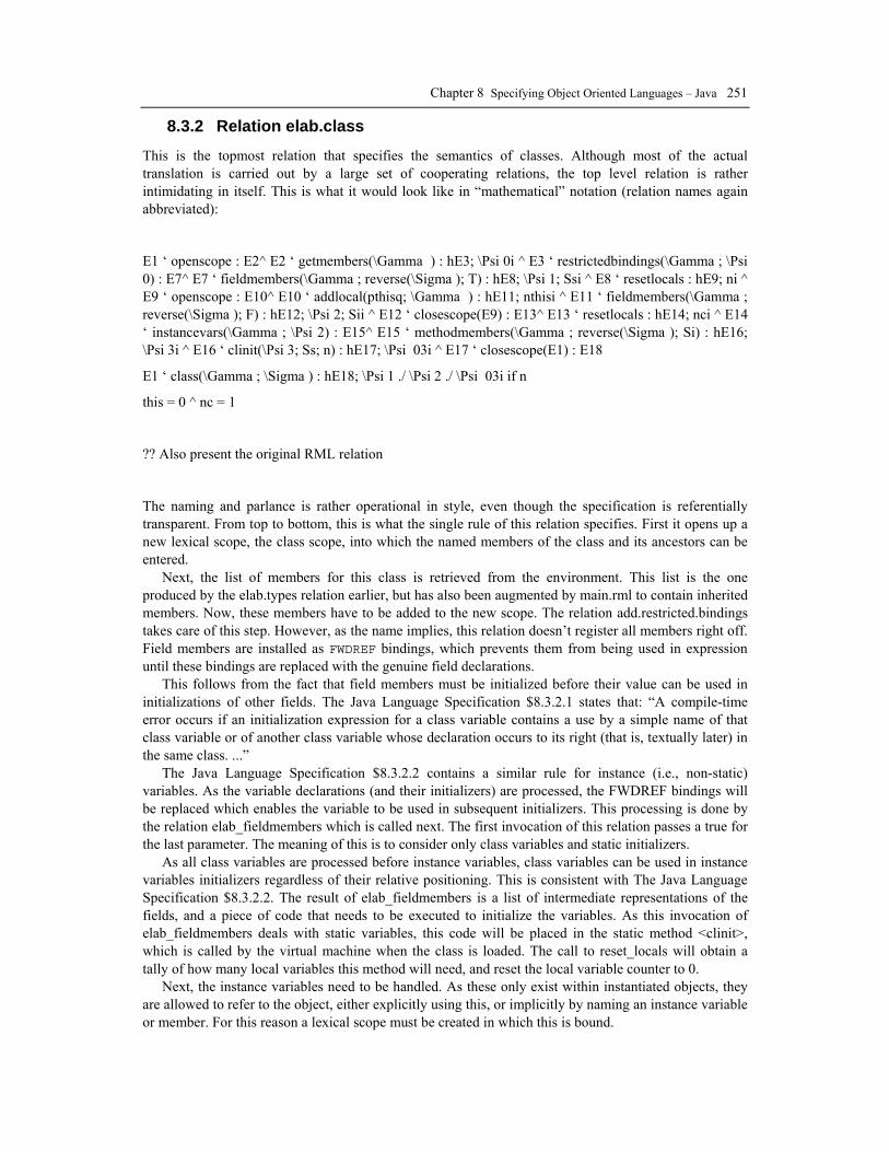
Chapter 8 Specifying Object Oriented Languages – Java 251
8.3.2 Relation elab.class
This is the topmost relation that specifies the semantics of classes. Although most of the actual translation is carried out by a large set of cooperating relations, the top level relation is rather intimidating in itself. This is what it would look like in “mathematical” notation (relation names again abbreviated):
E1 ‘ openscope : E2^ E2 ‘ getmembers(\Gamma ) : hE3; \Psi 0i ^ E3 ‘ restrictedbindings(\Gamma ; \Psi 0) : E7^ E7 ‘ fieldmembers(\Gamma ; reverse(\Sigma ); T) : hE8; \Psi 1; Ssi ^ E8 ‘ resetlocals : hE9; ni ^ E9 ‘ openscope : E10^ E10 ‘ addlocal(pthisq; \Gamma ) : hE11; nthisi ^ E11 ‘ fieldmembers(\Gamma ; reverse(\Sigma ); F) : hE12; \Psi 2; Sii ^ E12 ‘ closescope(E9) : E13^ E13 ‘ resetlocals : hE14; nci ^ E14 ‘ instancevars(\Gamma ; \Psi 2) : E15^ E15 ‘ methodmembers(\Gamma ; reverse(\Sigma ); Si) : hE16; \Psi 3i ^ E16 ‘ clinit(\Psi 3; Ss; n) : hE17; \Psi 03i ^ E17 ‘ closescope(E1) : E18
E1 ‘ class(\Gamma ; \Sigma ) : hE18; \Psi 1 ./ \Psi 2 ./ \Psi 03i if n
this = 0 ^ nc = 1
?? Also present the original RML relation
The naming and parlance is rather operational in style, even though the specification is referentially transparent. From top to bottom, this is what the single rule of this relation specifies. First it opens up a new lexical scope, the class scope, into which the named members of the class and its ancestors can be entered.
Next, the list of members for this class is retrieved from the environment. This list is the one produced by the elab.types relation earlier, but has also been augmented by main.rml to contain inherited members. Now, these members have to be added to the new scope. The relation add.restricted.bindings takes care of this step. However, as the name implies, this relation doesn’t register all members right off. Field members are installed as FWDREF bindings, which prevents them from being used in expression until these bindings are replaced with the genuine field declarations.
This follows from the fact that field members must be initialized before their value can be used in initializations of other fields. The Java Language Specification $8.3.2.1 states that: “A compile-time error occurs if an initialization expression for a class variable contains a use by a simple name of that class variable or of another class variable whose declaration occurs to its right (that is, textually later) in the same class. ...”
The Java Language Specification $8.3.2.2 contains a similar rule for instance (i.e., non-static) variables. As the variable declarations (and their initializers) are processed, the FWDREF bindings will be replaced which enables the variable to be used in subsequent initializers. This processing is done by the relation elab_fieldmembers which is called next. The first invocation of this relation passes a true for the last parameter. The meaning of this is to consider only class variables and static initializers.
As all class variables are processed before instance variables, class variables can be used in instance variables initializers regardless of their relative positioning. This is consistent with The Java Language Specification $8.3.2.2. The result of elab_fieldmembers is a list of intermediate representations of the fields, and a piece of code that needs to be executed to initialize the variables. As this invocation of elab_fieldmembers deals with static variables, this code will be placed in the static method <clinit>, which is called by the virtual machine when the class is loaded. The call to reset_locals will obtain a tally of how many local variables this method will need, and reset the local variable counter to 0.
Next, the instance variables need to be handled. As these only exist within instantiated objects, they are allowed to refer to the object, either explicitly using this, or implicitly by naming an instance variable or member. For this reason a lexical scope must be created in which this is bound.

252 Peter Fritzson Generation of Language Implementations from Structural and Natural Semantics
The invocations of open.scope and add.local that follow next provide this scope with the correct binding of this. (this is always local variable ?? 0 when it exists.) After this the instance
variables can be processed in the same way as the static variables. The final parameter to elab.fieldmembers is now false, to select non-static members only. It is known that the number of local variables will be only 1 (meaningthe single variable this), as local variables can not be declared in variable initializers but only in static initializers, and there are no static initializers that are non-static (obviously).
Now it would appear that all members, including the fields, have obtained their correct bindings within the class scope. This is however not the case. As an extra scope was introduced to hold the this variable, all instance variables will have been entered into this temporary scope and removed when it was closed. Thus they need to be added once again, and this is done using the add_instancevars relation.
The next step now that the class scope is complete, is to translate all the methods and constructors. This is done by the elab_methodmembers relation. The parameter iinit (for “instance initializers”) is the code generated for initializing the instance variables. It will be prepended to the code for each constructor that does not call another constructor in the same class. This ensures that the code will be executed exactly once as soon as an object of this class is constructed. If such initialization code exists for the class variables as well (i.e., sinit, for “static initializers”, is not a no-operation), the relation elab_clinit will add the necessary method <clinit>.
Finally, the class scope is closed and the definitive member list is constructed from the lists , and which contain the class variables, the instance variables, and the methods and constructors, respectively. This list is returned together with the possibly augmented environment.
8.4 Symbol table When a language allows identifiers, it can either allow declarations and uses of identifiers in arbitrary order, or it can require that the declaration of an identifier must syntactically precede all uses of that identifier. Many languages fall into the latter category, such as Pascal, but Java belongs to the former category.
Managing the symbol table in a translational language specification is quite straightforward. When translating a declaration, the (translation of the) declared entity is inserted into the table together with the identifier being declared. When translating a use, the entity is retrieved from the symbol table by searching for the used identifier.
If usage of an identifier is allowed before its declaration however, things get more complicated. If the same scheme as described above were to be used, situations would soon occur where a use of an identifier has to be translated but there is no information in the symbol table as to what entity, or even what kind of entity, this identifier denotes.
What we need to do is to make multiple passes over the source program, i.e., first translate all declarations and then all uses. This sounds simple enough until you realize that a declaration can also be a use. In Java for example, declarations of classes can use declarations of other classes through the inheritance mechanism. Declarations of class members can also use declarations of classes by using them as types for function parameters and return values etc.
Typically, what we will need to do is to first build a crude representation of the declarations, without looking at the uses of identifiers present in the said declarations. Then all declarations have to be re-examined in order to build a more complete translation of the declarations, using the first representation as a means of resolving the uses of identifiers in the declarations. After this step all statements (which only contain uses of identifiers) can be translated using the more detailed identifier information. Because we were using incomplete information to construct the detailed translation, it will not contain complete information either. Rather, symbolic references have to be used to some extent. However, doing so means that circular reference chains can be handled without special measures.

Chapter 8 Specifying Object Oriented Languages – Java 253
8.4.1 A Two Level Approach
The important thing when specifying the strategy outlined in the previous section is of course to select the crude declaration representation so that it can be created without looking at any other declarations, yet provides enough additional information for the second pass to be able to generate a detailed translation of all declarations.
In the case of Java, the first thing to note is that only identifiers corresponding to class declarations can be used in other declarations. Method and field declarations are contained within class declarations, rather than being referred to by name. This means that it is only necessary to make the crude translation for class declarations.
What is needed is therefore a way to uniquely describe a class so that this description can be used when translating the rest of the declarations. It is not possible to provide any detailed description at this point, so a tag for which we later can provide additional information has to do. Fortunately, Java provides precisely such a tagging mechanism through the concept of Fully Qualified Names. Each Java class has a unique name that can be constructed from the identifier used at the declaration of the class and the Fully Qualified Name of the package in which it is declared.
The crude representation of class declarations in the Java specification is thus just a mapping from identifier to Fully Qualified Name. During the second pass, identifiers representing classes used in declarations are translated using this mapping into the Fully Qualified Name of the actual classes. When all the declarations contained in a class have been translated in this way, they are grouped together into a description of the class, which is inserted into a second mapping which is indexed by the Fully Qualified Name of the class.
In this way, the symbol table becomes a two level structure where the detailed information is only available by first finding the appropriate Fully Qualified Name. This structure is maintained also when translating the statements of the program. The crude level will then be the local environment, where each identifier which is in scope is associated with a shallow description of the entity denoted by the identifier. One or more accesses to the detailed mapping may be necessary to translate the statement containing the identifier use.
An example: Consider the statement foo.bar(gazonk);. Here, the local environment may contain the information that foo is a local variable holding an object, and that the class of this object has a Fully Qualified Name of ecky.ecky.ecky.ecky.pikang.zoop.boing.goodem.zoo.owli.zhiv. A look in the detailed table under this name reveals the internal structure of the class, in particular that bar is indeed a declared method, taking one argument. The type of the argument is provided through the Fully Qualified Name of the class, in this case wooden.badger. Going back to the local environment we can next discover that gazonk is another local variable holding an object of the class with the Fully Qualified Name holy.hand.grenade. Again, we must check the detailed table to find out whether holy.hand.grenade is a subclass of wooden.badger which is the requirement for this call to be legal.
8.5 Large Scale Library Environment In a real program, it is seldom enough to use only the primitive operations of the language. In order to perform common tasks, it is customary that references are made to an environment of standard libraries provided by the language implementation. This is especially true for Java in which even basic data types such as strings and dynamic arrays are provided only as library classes. It is therefore necessary for a formal specification to take the possibility of library calls into account.
In a strongly typed language, the types of the actual parameters must be checked against the formal parameters of each function call. This is of course true also for library calls. The type checking rules of the specification should therefore be able to retrieve type information from the library environment in order to enforce the type rules. In the case of Java, not only formal parameter types should be collected,

254 Peter Fritzson Generation of Language Implementations from Structural and Natural Semantics
but complete information about the names and types of the members (fields and methods) and constructors of each library class used, so that name resolution can take place properly.
More often than not, the source to the library environment is unavailable. And even if it were available, it would be a waste of effort to analyze the semantics of the library code for each program. Instead, a more compact representation of just the prototypes for the code, in binary format or otherwise, will be used. Java stores this information in binary format in the precompiled .class-files. By browsing through the .class-files available in the system’s CLASSPATH, it is possible to obtain all the necessary information about the library environment.
8.5.1 Lazy Access of Library Definitions
The library environment of Java has grown fairly large of late (Java 1.2 contains about 2200 library classes), which makes the task of gathering all prototype information available expensive. Also, the library classes are generally only available in compressed form, and need to be decompressed in order to be analyzed. This further slows down the startup of an implementation based on the principle to examine the entire environment.
As only a small part of the library environment is generally used by a particular application, a more efficient approach is to analyze only the library classes that are actually used. One way to do this would be to examine the source files and try to determine what classes are used before starting the actual translation. The name resolution rules of Java makes this difficult to do, though. It is not possible to determine exactly what classes are used without actually performing most of the translation steps.
The method actually used in the Java specification is therefore slightly different. Translation of the program starts right away, without analyzing any library classes. (An inventory of what library classes are available is first taken though.) As soon as a translation step determines that a library class is used and information about the class is needed, it invokes a special relation find_class. This relation will cause the class to be loaded and analyzed, and the information is returned. The translation can then proceed using this information. The next time the class is referred to in the source, find_class is invoked again. This time, the information collected on the last invocation is retrieved directly from a cache, eliminating the need to load and analyze the class again.
The cache is maintained within the translation environment, a structure that is passed between the translation relations, and updated with symbol table information and such. The drawback of placing the cache here is that if a precondition for a rule does not hold, and the system has to backtrack, information about classes loaded during the execution branch that is backtracked is lost. This is not a major problem, as it can generally be avoided by placing relation invocations that may cause classes to be loaded as far down in the execution tree as possible, thus minimizing the risk of them being backtracked over. Placing the cache in the translation environment also causes the structure of the specification to change slightly, as some relations that would not normally need to modify the environment have to return an updated environment because it can cause new classes to be added to the cache.
An alternate method would have been to have the cache in a global variable. The concept of global variables does not fit very well with the Structured Operational Semantics paradigm though, which is why this solution was avoided. One can argue that on demand loading to a cache does not fit very well into that paradigm either, but it is at least a tradeoff that can be motivated by greatly improved performance of implementation.
8.6 Use of RML Evaluation Order in the Specification In specifications of programming languages, it is common to have rules in which a number of preconditions are tested in order. As soon as one is satisfied the semantics of the particular program segment can be determined. In these cases, it is desirable to only describe each precondition and the

Chapter 8 Specifying Object Oriented Languages – Java 255
consequences of it holding. To explicitly state that all of the previous preconditions must not hold is cumbersome and also redundant, as rules stating what happens if they do hold have already been given.
In RML, the rules of a relation which have the same term structure are tested in lexicographic order, which means that a rule is only tested if the preconditions have failed to hold for all the rules with the same term structure that precedes the rule textually. This means that our intuition of fall-back rules can easily be implemented by simply placing the rules in the correct order, with the most specific case first. The downside is of course that the result of a rule no longer follows logically from the terms and preconditions, but it is possible to imagine an augmented specification in which the preconditions of each rule is extended with the inverse preconditions of each textually preceding rule for the relation. This augmented specification is an equivalent RML program in which the result for each rule follows directly from the preconditions and terms.
8.6.1 An example
For an example of the usefulness of exploiting the evaluation order of RML in this way, consider the ?: operator of Java. The type rules of this operator (as specified in The Java Language Specification[2??]) are:
The type of a conditional expression is determined as follows:
• If the second and third operands have the same type (which may be the null type), then that is the type of the conditional expression.
• Otherwise, if the second and third operands have numeric type, then there are several cases: • If one of the operands is of type byte and the other is of type short, then the type of the
conditional expression is short. • If one of the operands is of type T where T is byte, short, or char, and the other operand is a
constant expression of type int whose value is representable in type T, then the type of the conditional expression is T.
• Otherwise, binary numeric promotion (Java Language Specification $5.6.2) is applied to the operand types, and the type of the conditional expression is the promoted type of the second and third operands.
• If one of the second and third operands is of the null type and the type of the other is a reference type, then the type of the conditional expression is that reference type.
• If the second and third operands are of different reference types, then it must be possible to convert one of the types to the other type (call this latter type T ) by assignment conversion (Java Language Specification $5.2); the type of the conditional expression is T. It is a compile-time error if neither type is assignment compatible with the other type.
Notice the use of the word “otherwise” on two levels. Should a rule that in itself expresses exactly when binary numeric promotion is to used be constructed, its preconditions would have to verify that:
• The second and third argument are not of the same type • The second and third argument are both of numeric types • It is not the case that the second argument is of type byte and the third argument is of type short • It is not the case that the second argument is of type byte, short or char, and the the third
argument is a constant expression of type int, the value of which is representable in the type of the second argument
• It is not the case that the third argument is of type byte, short or char, and the the second argument is a constant expression of type int, the value of which is representable in the type of the third argument
Several of these preconditions are quite complex and would cause the rule to look incomprehensible to a human eye. On the other hand, if the more relaxed approach of relying on the evaluation order of RML is used, most of these preconditions can be omitted, given that the more specific rules are given first. If
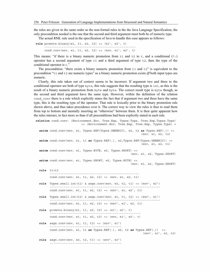
256 Peter Fritzson Generation of Language Implementations from Structural and Natural Semantics
the rules are given in the same order as the non-formal rules in the the Java Language Specification, the only precondition needed is the one that the second and third argument must both be of numeric type.
The actual RML rule used in the specification of Java to handle this case appears as follows: rule promote.binary(e1, t1, e2, t2) => (e1’, e2’, t) ---------------------------------------------------- cond.conv(env, e1, t1, e2, t2) => (env, e1’, e2’, t)
This means: “if there is a binary numeric promotion from t1 and t2 to t, and a conditional (?:) operator has a second argument of type t1 and a third argument of type t2, then the type of the conditional operator is t.”
The precondition: “there exists a binary numeric promotion from t1 and t2” is equivalent to the precondition “t1 and t2 are numeric types” as a binary numeric promotion exists iff both input types are numeric.
Clearly, this rule taken out of context seems to be incorrect. If argument two and three to the conditional operator are both of type byte, this rule suggests that the resulting type is int, as this is the result of a binary numeric promotion from byte and byte. The correct result type is byte though, as the second and third argument have the same type. However, within the definition of the relation cond_conv there is a rule which explicitly states the fact that if argument two and three have the same type, this is the resulting type of the operator. That rule is lexically prior to the binary promotion rule shown above, and thus takes precedence over it. The correct way to view the rules is thus to read them from top to bottom and mentally inserting an “otherwise” between them. It is then quite apparent how the rules interact, in fact more so than if all preconditions had been explicitly stated in each rule. relation cond.conv: (Environment.Env, Tree.Exp, Types.Type, Tree.Exp,Types.Type) => (Environment.Env, Tree.Exp, Tree.Exp, Types.Type) = axiom cond.conv(env, e1, Types.REF(Types.GENERIC), e2, t2 as Types.REF(.)) => (env, e1, e2, t2) axiom cond.conv(env, e1, t1 as Types.REF(.), e2,Types.REF(Types.GENERIC)) => (env, e1, e2, t1) axiom cond.conv(env, e1, Types.BYTE, e2, Types.SHORT) => (env, e1, e2, Types.SHORT) axiom cond.conv(env, e1, Types.SHORT, e2, Types.BYTE) => (env, e1, e2, Types.SHORT) rule t1=t2 --------------------------------------------------- cond.conv(env, e1, t1, e2, t2) => (env, e1, e2, t1) rule Types.small.int(t1) & asgn.conv(env, e2, t2, t1) => (env’, e2’) --------------------------------------------------------------- cond.conv(env, e1, t1, e2, t2) => (env’, e1, e2’, t1) rule Types.small.int(t2) & asgn.conv(env, e1, t1, t2) => (env’, e1’) --------------------------------------------------------------- cond.conv(env, e1, t1, e2, t2) => (env’, e1’, e2, t1) rule promote.binary(e1, t1, e2, t2) => (e1’, e2’, t) ---------------------------------------------------- cond.conv(env, e1, t1, e2, t2) => (env, e1’, e2’, t) rule asgn.conv(env, e1, t1, t2) => (env’, e1’) ----------------------------------------- cond.conv(env, e1, t1 as Types.REF(.), e2, t2 as Types.REF(.)) => (env’, e1’, e2, t2) rule asgn.conv(env, e2, t2, t1) => (env’, e2’) -----------------------------------------

Chapter 8 Specifying Object Oriented Languages – Java 257
cond.conv(env, e1, t1 as Types.REF(.), e2, t2 as Types.REF(.)) => (env’, e1, e2’, t1) end
8.6.2 Value Domains of Specification Language and Specified Language
A computer language typically contains some form of arithmetic evaluation. While it is possible to use Structured Operational Semantics to describe the arithmetic itself (for example using Peano arithmetic), it is usually not necessary or desirable to do so. Instead, arithmetic operations built into the specification language can be used. Doing so will dramatically improve performance of the generated implementation, and will also make the rules look more familiar to a human reader.
When using builtin operators of the specification language to describe the semantics of the specified language, it is of course important that the semantics of the builtin operators is known, and preferably similar to those of the operators in the specified language. Generally, this is not a big problem, arithmetic operations such as addition have fairly standardized semantics in most languages (??specification- and specified).
However, the domains on which these operators apply may vary. Numeric operators are generally defined on builtin numeric types provided by the language, and the range of the types provided by the specification language may be different from those of the specified language. In order to use a builtin addition operator to determine the value of an arithmetic expression in the specified language such as a+b, where a, b and a+b are all representable in the abstract syntax defined as a union type for representing the specified language, these values must also be representable in the domain supported by the builtin addition operator.
This is not just true for arithmetic operations. Wherever it is desirable to use builtin operators of the specification language to resolve expressions dealing with data items belonging to the specified language, it is necessary to examine the value domains of the language concerned to ensure that the result indeed confirms with the semantics of the specified language. Besides numeric types for arithmetic calculations, there may for example be string types on which one needs to perform operations such as concatenation.
Integer arithmetic in Java occurs in the 32-bit and 64-bit domains, whereas RML originally only provided 31-bit integers. However it was possible to introduce an external 64-bit long integer data type by creating an extension module.
Another approach is to map the value domain of the subject language data type into some domain available in the specification language. This was done for Java’s 16-bit strings, which were mapped to 8-bit RML strings using UTF-8.
8.7 Suggestions for Extensions to RML Although RML is already a powerful system for expressing programming language semantics, there are some possibilities for improvement. Here are a few extensions based on current experience that could be desired from future RML versions.
8.7.1 Named Arguments in Pattern Matching and Construction
A common operation is matching on a single argument in a larger structure, and then replacing this argument with an updated value in a new structure. This would typically appear as the example below in RML: ???

258 Peter Fritzson Generation of Language Implementations from Structural and Natural Semantics
In order to maintain state such as symbol table and the internal structure of classes being translated, a special environment structure is used in the Java specification. This structure is aggregated from a set of sub-states that are used at different times for different purposes. The current symbol table is one such sub-state, for example. A number of operations have been defined on the environment, so that the rest of the rules do not have to bother with the internal structure of the environment. Still, these operations need to extract the sub-state on which to operate, do whatever it is supposed to do, and then reassemble the environment with the new sub-state in place. This generally results in a great deal of code that appears as follows: rule do.something(s1) => s2 ---------------------------------------------------------- some.operation(ENV(x,y,z,s1,u,v,w)) => ENV(x,y,z,s2,u,v,w)
It would be possible to write this in a shorter notation that is also independent of the exact order of arguments to ENV if named arguments were supported. If the argument used above (number 4 from the left) was named Sub1, a rule like the following might be possible: ??(missing rule)
Apart from being tedious to write, this rule obviously has to be rewritten if one more sub-state is added to the ENV structure. A possible solution to this problem would be to be able to name the components of a structure, and then use this name in pattern matching and when constructing new instances of the structure.
For example, if ENV has seven components, as above, and the fourth component has been named Sub1, the matching pattern ENV(Sub1 => s1) might mean the same as ENV(.,.,.,s1,.,.,.). (. means match any value.) Even if the number of components in ENV changes, this pattern will remain legal as long as Sub1 remains.
In order to construct new environments like ENV without having to know exactly what the components are, a default must be provided for the components that are not explicitly given values. This should be done by specifying an existing ENV structure, typically the result of the partial match described above, in which to substitute zero or more components. The syntax for this might be for example Sub1 => s2, where e is the old ENV structure, and s2 is the new value for the Sub1 component. The example rule above would then look appear as follows: rule do.something(s1) => s2 ------------------------------------------------------ some.operation(e as ENV(Sub1 => s1)) => ??????e\(Sub1 => s2)
This rule is easier to read, easier to write, and will keep working even if new substates are introduced to the environment structure.
8.7.2 Lazy evaluation
In the section “Library Environment” above, a situation was discussed in which a large amount of data to process was available, not all of which was necessarily needed in processed form. However, by delaying the processing until it has been deemed necessary, there is a risk of doing the same processing twice instead. A cache can be used to reduce this risk, but is not a very aesthetically pleasing solution, and when backtracking can occur not always an efficient one.
For this situation, the concept of lazy evaluation would really come in handy. Instead of doing all the processing in advance, and instead of manually delaying the processing, all the processing could be requested to be done lazily. For this to work in RML, some operation to delay and force evaluation would be required. Such operations are supported by several implementations of Standard ML, including Standard ML of New Jersey, as well as implicitly in lazy functional languages such as Haskell.
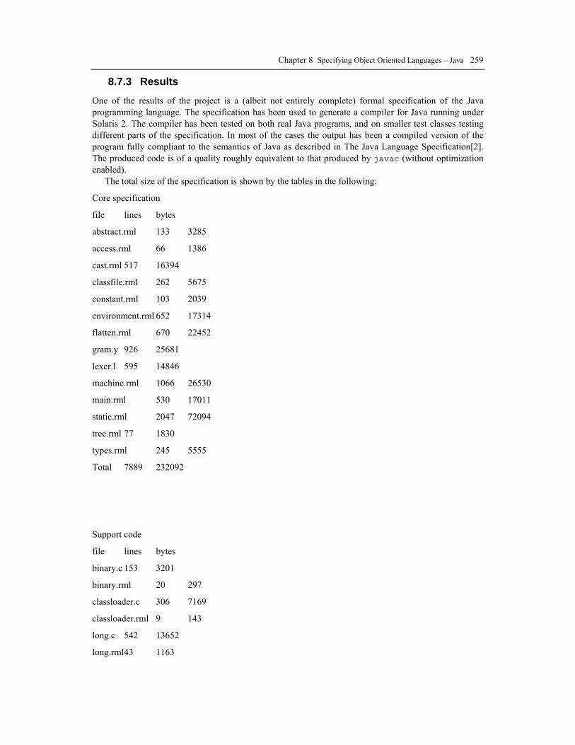
Chapter 8 Specifying Object Oriented Languages – Java 259
8.7.3 Results
One of the results of the project is a (albeit not entirely complete) formal specification of the Java programming language. The specification has been used to generate a compiler for Java running under Solaris 2. The compiler has been tested on both real Java programs, and on smaller test classes testing different parts of the specification. In most of the cases the output has been a compiled version of the program fully compliant to the semantics of Java as described in The Java Language Specification[2]. The produced code is of a quality roughly equivalent to that produced by javac (without optimization enabled).
The total size of the specification is shown by the tables in the following:
Core specification
file lines bytes
abstract.rml 133 3285
access.rml 66 1386
cast.rml 517 16394
classfile.rml 262 5675
constant.rml 103 2039
environment.rml 652 17314
flatten.rml 670 22452
gram.y 926 25681
lexer.l 595 14846
machine.rml 1066 26530
main.rml 530 17011
static.rml 2047 72094
tree.rml 77 1830
types.rml 245 5555
Total 7889 232092
Support code
file lines bytes
binary.c 153 3201
binary.rml 20 297
classloader.c 306 7169
classloader.rml 9 143
long.c 542 13652
long.rml 43 1163

260 Peter Fritzson Generation of Language Implementations from Structural and Natural Semantics
mkunicodemap.c 182 3937
my_unify.c 80 2083
parser.c 43 929
parser.rml 10 129
Total 1388 32703
8.7.4 Extensibility
The specification is fairly simple to extend, by virtue of being written in a declarative style. Although there are not many comments in the source, most of the relations have reasonably describing names and a brief study of the existing code should make their use apparent. The modular approach used also promotes extensibility by partitioning the specification into independent blocks sharing only a minimal interface.
8.7.5 Experienced Performance
How well does an implementation generated from an RML translational specification perform in comparison to a traditional hand-written compiler? Well, obviously the performance cannot be expected to be better than that of the handwritten compiler, but in fact it is not that much worse either. The following table compares compilation times of a few Java source files. RML is the time for the compiler generated from the Structured Operational Semantics specification in RML, javac is the time for the javac compiler running on the Java Virtual Machine provided by Sun’s JDK1.1.1, and jit is the time for the same javac, running on the same Java Virtual Machine with the Just In Time compiler enabled. All times are averages of 10 runs, and the machine used in the test is a Sun Ultra-1.
Measured compilation times (?? made year 2000) for the RML-based generated Java compiler, Suns javac, and Suns jit compiler.
file #lines RML javac jit
blank.java 2 0.78s 1.75s 1.60s
hello.java 6 1.18s 1.95s 1.87s
gissa.java 35 1.61s 2.73s 2.85s
BorderLayout.java 376 5.10s 3.05s 2.96s
It can be noted that the generated translator has a shorter startup time, which accounts for the better performance on the really short files. The performance on larger files tested is not below 50% that of Javac.
The specification currently makes use of rather simplistic structures for environment structures such as symbol tables. More complex structures with powerful access operators would probably improve performance for larger programs.
Chapter 8 Specifying Object Oriented Languages – Java 261
8.8 Conclusions This Chapter describes some aspects of a full scale Structured Operational Semantics specification of a real-world programming language (Java) and experiences from generating a compiler from this specification. Some observations are summarized below:
Having a two level symbol table simplifies handling of forward references in type declarations. Analyzing predefined libraries on demand and storing the results in a cache can improve
performance. The use of lazy evaluation can make the cache implicit which gives better readability and transparency.
Exploiting procedural properties such as the order of rule evaluation in the specification language can give shorter and more readable rules, but makes it harder to view the specification as just a set of logical implications.
If the specification needs to deal with data types in the specified language that are not available in the specification language, such types can either be introduced into the specification language or mapped onto types present in the specification language.
A compiler generated from a Structured Operational Semantics specification in RML has reasonable performance compared to a traditional compiler.
A mechanism for naming arguments to RML constructors and using these names in pattern matches would have made the specification shorter, more readable and easier to extend.
8.9 References Marcus Comstedt. Natural Semantics Specification and Compiler Generation for Java. Master Thesis LITH-IDA-Ex-97/44. Linköping University, 1997.
Mikael Holmén. Natural Semantics Specification and Frontend Generation for Java 1.2. Master Thesis LITH-IDA-Ex-00/60. Linköping University, 2000.
James Gosling, Bill Joy, and Guy Steele. The Java Language Specification. Addison Wesley Publishing Company, 1996.
Gilles Kahn, Natural Semantics. In Proceedings of the Symposium on Theoretical Aspects of Computer Science, STACS’87, Vol. 247 of LNCS, pp. 22-39. Springer Verlag, 1987.
Tim Lindholm and Frank Yellin. The Java Virtual Machine Specification. Addison Wesley Publishing Company, 1997.
Robin Milner, Mads Tofte, and Robert Harper. The Definition of Standard ML. The MIT Press, Cambridge, Massachusetts, 1990.
Frank G. Pagan. Formal Specification of Programming Languages: A Panoramic Primer. Prentice-Hall, 1981.
Mikael Pettersson. Compiling Natural Semantics. Ph.D. thesis, Linköping University, Dec 1995. To appear as a volume in LNCS, Springer-Verlag. (?? update reference)
?? Also add reference to a book containing a Java specification

263
Chapter 9 Specifying Modelica—a Declarative Object-Oriented Equation-Based Language
Modelica (??Fritzson 2003) is an object-oriented language for modeling of physical systems for the purpose of efficient simulation. The language unifies and generalizes previous object-oriented modeling languages.
Compared with the widespread simulation languages available today this language offers three important advances:
• 1) non-causal modeling based on differential and algebraic equations; • 2) multidomain modeling capability, i.e., it is possible to combine electrical, mechanical,
thermodynamic, hydraulic etc. model components within the same application model; • 3) a general type system that unifies object-orientation, multiple inheritance, and templates
within a single class construct.
A Modelica model is defined in terms of classes containing equations and definitions. The semantics, i.e., the meaning of such a model is defined via translation of classes, instances, connections and functions into a flat set of constants, variables and equations. Equations are sorted and converted to assignment statements when possible. Strongly connected sets of equations are solved by calling a symbolic and/or numeric solver.
9.1 Modelica View of Object-orientation Traditional object-oriented languages like C++, Java, and Simula support programming with operations on state. The state of the program includes variable values and object data, and the number of objects may change dynamically. The Modelica approach is different. The Modelica language emphasizes structured mathematical modeling and uses the structural benefits of object orientation. A Modelica model is primarily a declarative mathematical description, which allows analysis and equational reasoning. For these reasons, dynamic object creation at runtime is usually not interesting from a mathematical modeling point of view, and is currently not supported by the Modelica language.
For other reasons, and to compensate this missing feature arrays are provided by Modelica. An array is an indexed set of objects of equal type. The size of the set is determined once at runtime. This construct for example can be used to represent a set of similar rollers in a bearing, or a set of electrons around an atomic nucleus.
9.1.1 Object-Oriented Mathematical Modeling
Mathematical models used for analysis in scientific computing are inherently complex in the same way as other software. One way to handle this complexity is to use object-oriented techniques.
However, there are some fundamental differences between object-oriented programming and object-oriented mathematical modeling, where a class description may consist of a set of equations, which implicitly define the behavior of some class of physical objects or the relationships between objects. Functions should be side-effect free and are regarded as mathematical functions rather than operations

264 Peter Fritzson Generation of Language Implementations from Structural and Natural Semantics
on objects. Explicit operations on state may be completely absent, but may also be present. Also, causality, i.e., which variables are regarded as input, and which are regarded as output, is usually not defined by such an equation-based model.
There are usually many choices of causality, but one must be selected prior to solving a system of equations. If a system of such equations is solved symbolically, i.e., solved statically once and for all at compile time, the equations are transformed into a form where some (state) variables are explicitly defined in terms of other (state) variables. If the solution process is dynamic at run-time, it will compute new state variables from old variable values, and thus operate on the state variables.
9.2 Modelica Fundamentals Modelica models are built from classes. Like in other object-oriented languages, a class contains variables, i.e., class attributes representing data. The main difference compared to traditional object-oriented languages is that instead of functions (methods) we use equations to specify behavior.
Equations can be written explicitly, like a=b, or be inherited from other classes. Equations can also be specified by the connect construct. The special equation construct connect(v1,v2) expresses coupling between variables v1 and v2. These variables are called connectors in Modelica parlance, i.e., ports or interfaces, and belong to the connected objects. This gives a flexible way of specifying topology of physical systems described in an object-oriented way using Modelica.
In the following sections we briefly introduce some basic and distinctive syntactic and semantic features of Modelica, such as connectors, encapsulation of equations, inheritance, declaration of model parameters and constants, as well as powerful parametrization capabilities.
9.2.1 The Modelica Notion of Subtypes
The notion of subtyping in Modelica is influenced by the type theory of Abadi and Cardelli (??Abadi and Cardelli 1996). The notion of inheritance in Modelica is separated from the notion of subtyping. According to the definition, a class A is a subtype of class B if class A contains all the public variables declared in the class B, and types of these variables are subtypes of the types of corresponding variables in B. The main benefit of this definition is additional flexibility in the composition of types. For instance, the class TempResistor is a subtype of Resistor.
Note that the keyword parameter is used in Modelica for a special kind of constants that are do not change during simulation, but can be changed before or between simulations. Such parameters will in the following be called model parameters to avoid confusion compared to formal parameters to functions and RML relations.. class Resistor extends TwoPin parameter Real R; equation v=R*i; end Resistor; class TempResistor extends TwoPin parameter Real R, RT, Tref; Real T; equation v=i*(R+RT*(T-Tref)); end TempResistor
Subtyping is used for example in class instantiation, redeclarations , and function calls. If variable a is of type A, and A is a subtype of B, then a can be initialized by a variable of type B.

Chapter 9 Specifying Modelica—a Declarative Object-Oriented Equation-Based Language 265
Note that TempResistor does not inherit the Resistor class. There are different equations for evaluation of v. If equations would be inherited from Resistor then the set of equations will become inconsistent in TempResistor, since Modelica currently does not support named equations (except definition equations) and replacement of equations. For example, the specialized equation below from TempResistor: v=i*(R+RT*(T-Tref))
and the general equation from class Resistor: v=R*i
are inconsistent, and should not occur simulaneously in the same class.
9.3 Class Parametrization A distinctive feature of object-oriented programming languages and environments is the ability to fetch classes from standard libraries to be reused for particular needs. Such reuse should be done without modification of the library codes. The two main mechanisms for reuse are:
• Inheritance. This is essentially “copying” class definition and adding additional elements (variables, equations and functions).
• Class parametrization. (Also known as generic classes or generic types.) This replaces a generic type identifier in the whole class definition by an actual type.
Modelica contains a way to control class parametrization. Assume that a library class is defined as follows: class SimpleCircuit Resistor R1(R=100), R2(R=200); Resistor R3(R=300); equation connect(R1.p, R2.p); connect(R1.p, R3.p); end SimpleCircuit;
Assume that in our particular application we would like to reuse the definition of SimpleCircuit: we want to use the model parameter values given for R1.R and R2.R and the circuit topology, but exchange Resistor with the temperature-dependent resistor model, c, discussed above.
This can be accomplished by redeclaring R1 and R2 as follows. class RefinedSimpleCircuit = SimpleCircuit( redeclare TempResistor R1, redeclare TempResistor R2 );
The result is equivalent to the following expanded class: class SimpleCircuitExpanded TempResistor R1(R=100), R2(R=200); Resistor R3(R=300); equation connect(R1.p, R2.p); connect(R1.p, R3.p); end SimpleCircuit;
Since TempResistor is a subtype of Resistor, it is possible to replace the ideal resistor model. Values of the additional model parameters of TempResistor can also be added in the redeclaration, as in the following example: redeclare TempResistor R1(RT=0.1, Tref=20.0)
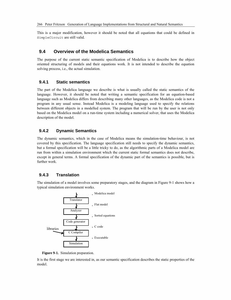
266 Peter Fritzson Generation of Language Implementations from Structural and Natural Semantics
This is a major modification, however it should be noted that all equations that could be defined in SimpleCircuit are still valid.
9.4 Overview of the Modelica Semantics The purpose of the current static semantic specification of Modelica is to describe how the object oriented structuring of models and their equations work. It is not intended to describe the equation solving process, i.e., the actual simulation.
9.4.1 Static semantics
The part of the Modelica language we describe is what is usually called the static semantics of the language. However, it should be noted that writing a semantic specification for an equation-based language such as Modelica differs from describing many other languages, as the Modelica code is not a program in any usual sense. Instead Modelica is a modeling language used to specify the relations between different objects in a modelled system. The program that will be run by the user is not only based on the Modelica model on a run-time system including a numerical solver, that uses the Modelica description of the model.
9.4.2 Dynamic Semantics
The dynamic semantics, which in the case of Modelica means the simulation-time behaviour, is not covered by this specification. The language specification still needs to specify the dynamic semantics, but a formal specification will be a little tricky to do, as the algorithmic parts of a Modelica model are run from within a simulation environment which the current static formal semantics does not describe, except in general terms. A formal specification of the dynamic part of the semantics is possible, but is further work.
9.4.3 Translation
The simulation of a model involves some preparatory stages, and the diagram in Figure 9-1 shows how a typical simulation environment works.
Modelica model
Flat model
Sorted equations
C code
Executable
Translator
Analyzer
Code generator
C Compiler
Simulation
libraries
Figure 9-1. Simulation preparation.
It is the first stage we are interested in, as our semantic specification describes the static properties of the model.
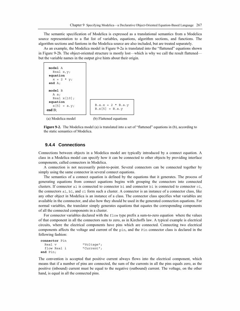
Chapter 9 Specifying Modelica—a Declarative Object-Oriented Equation-Based Language 267
The semantic specification of Modelica is expressed as a translational semantics from a Modelica source representation to a flat list of variables, equations, algorithm sections, and functions. The algorithm sections and funtions in the Modelica source are also included, but are treated separately.
As an example, the Modelica model in Figure 9-2a is translated into the “flattened” equations shown in Figure 9-2b. The object-oriented structure is mostly lost—which is why we call the result flattened— but the variable names in the output give hints about their origin.
model A Real x,y; equation x = 2 * y; end A; model B A a; Real x[10]; equation x[5] = a.y;
end B;
(a) Modelica model (b) Flattened equations
B.a.x = 2 * B.a.y B.x[5] = B.a.y
Figure 9-2. The Modelica model (a) is translated into a set of “flattened” equations in (b), according to the static semantics of Modelica.
9.4.4 Connections
Connections between objects in a Modelica model are typically introduced by a connect equation. A class in a Modelica model can specify how it can be connected to other objects by providing interface components, called connectors in Modelica.
A connection is not necessarily point-to-point. Several connectors can be connected together by simply using the same connector in several connect equations.
The semantics of a connect equation is defined by the equations that it generates. The process of generating equations from connect equations begins with grouping the connectors into connected clusters. If connector a1 is connected to connector b1 and connector b1 is connected to connector c1, the connectors a1, b1, and c1 form such a cluster. A connector is an instance of a connector class, like any other object in Modelica is an instance of a class. The connector class specifies what variables are available in the connnector, and also how they should be used in the generated connection equations. For normal variables, the translator simply generates equations that equates the corresponding components of all the connected components in a cluster.
For connector variables declared with the flow type prefix a sum-to-zero equation where the values of that component in all the connectors sum to zero, as in Kirchoffs law. A typical example is electrical circuits, where the electrical components have pins which are connected. Connecting two electrical components affects the voltage and current of the pin, and the Pin connector class is declared in the following fashion: connector Pin Real v "Voltage"; flow Real i "Current"; end Pin;
The convention is accepted that positive current always flows into the electrical component, which means that if a number of pins are connected, the sum of the currents in all the pins equals zero, as the positive (inbound) current must be equal to the negative (outbound) current. The voltage, on the other hand, is equal in all the connected pins.

268 Peter Fritzson Generation of Language Implementations from Structural and Natural Semantics
9.4.5 Parameterization
In most cases model parameters in a Modelica model are unproblematic, and the translator can simply emit a flat model with the model parameters still available as model parameters that can be given different values during equation solving. But in some cases this is not so. We differentiate between two types of model parameters, structural model parameters, which affect the number and content of the equations, and value model parameters, that do not.
One simple example of a structural model parameter is when a model parameter is used in the size of an array. Consider the following model: model ArrayEx parameter Real N = 3; Real a[N]; equation a[1] = 1; for i in 2:N loop a[i] = a[i-1] * 2; end for; end ArrayEx;
This will, with the model parameter N unmodified, produce the following equations: a[1] = 1 a[2] = 2 a[3] = 4
However, if the model parameter N is modified to be 5 when the model is instantiated, the set of equations will be different: a[1] = 1 a[2] = 2 a[3] = 4 a[4] = 8 a[5] = 16
As the semantic specification specifies the semantics in terms of the generated equations, this means that the value of the model parameters need to be determined to make it possible for the translator to do the translation.
Another, even more serious, complication with model model parameters is the combined use of model model parameters and connect-equations. If a model for example contains a connect equation that looks like connect(a[N],c), where a is an array of connectors, and N is a model model parameter, then the generated equations may look very different depending on the value of N. Not only the number of equations may change, but the equations themselves can be altered.
9.5 The Static Semantics Specification The specification is separated into a number of modules, to separate different stages of the translation, and to make it more manageable. This section will cover the most important parts of the specification. In all, the specification contains approximately thirty thousand (44 000 lines??) lines of RML, but it should be kept in mind that the RML code is rather sparse, with many empty or short lines, so that it is easier on human eyes.
The top level relation in the semantics is called main, and appears as follows: relation main =
rule Parser.parse(f) => p & SCode.elaborate(p) => p’ & Inst.instantiate(p’) => d & DAE.dump(d) & ----------------

Chapter 9 Specifying Modelica—a Declarative Object-Oriented Equation-Based Language 269
main( [f] ) end
9.5.1 Parsing and Abstract Syntax
The relation Parser.parse is actually written in C, and calls the parser generated from a grammar by the ANTLR parser generator tool (??ANTLR ??PCCTS 1998). This parser builds an abstract syntax tree from the source file, using the abstract syntax tree data types in a RML module calles Absyn. The parsing stage is not really part of the semantic description, but is of course necessary to build a real translator.
9.5.2 Rewriting the Abstract Syntax Tree
The abstract syntax tree closely corresponds to the parse tree and keeps the structure of the source file. This has several disadvantages when it comes to translating the program, and especially if the translation rules should be easy to read for a human. For this reason a preparatory translation pass is introduced which translates the abstract syntax tree into an intermediate form, called SCode. Besides some minor simplifications the SCode structure differs from the abstract syntax tree in the following respects:
• All variables are described separately. In the source code and in the abstract syntax tree several variables in a class definition can be declared at once, as in Real x, y[17];. In the SCode this is represented as two unrelated declarations, as if it had been written Real x; Real y[17];.
• Class declaration sections. In a Modelica class declaration the public, protected, equation, and algorithm sections may be included in any number and in any order, with an implicit public section first. In the SCode these sections are collected so that all public and protected sections are combined into one section, while keeping the order of the elements. The information about which elements were in a protected section is stored with the element itself.
One might have thought that more work could be done at this stage, like analyzing expression types and resolving names. But due to the nature of the Modelica language, the only way to know anything about how the names will be resolved during code instantiation is to do a more or less full code instantiation. It is possible to analyze a class declaration and find out what the parts of the declaration would mean if the class was to be instantiated as-is, but since it is possible to modify much of the class while instantiating it that analysis would not be of much use.
9.5.3 Code Instantiation
The central part of the translation is instantiating the code of the model. The convention is that the top-level model in the source file is instantiated, which means that the equations in that model declaration, and all its subcomponents, are calculated and collected.
The instantiation of a class is done by looking at the class definition, instantiating all subcomponents and collecting all equations. To accomplish this, the translator needs to keep track of the class context. The context includes the lexical scope of the class definition. This constitutes the environment which includes the variables and classes declared previously in the same scope as the current class, and its parent scope, and all enclosing scopes. The other part of the context is the current set of modifiers which modify things like model model parameter values or redeclare subcomponents. model M constant Real c = 5;
model Foo parameter Real p = 3; Real x;

270 Peter Fritzson Generation of Language Implementations from Structural and Natural Semantics
equation x = p * sin(time) + c; end Foo; Foo f(p = 17); end M;
In the example above, instantiating the model M means instantiating its subcomponent f, which is of type Foo. While instantiating f the current environment is the parent environment, which includes the constant c. The current set of modifications is (p = 17), which means that the model parameter p in the component f will be 17 rather than 3.
There are many semantic rules that takes care of this, but only a few are shown in inst_class. They are also somewhat simplified to focus on the central aspects. relation inst_class =
rule Env.open_scope(env) => env’ & inst_class_in(env’,mod,pre,csets,c) => (dae1,_,csets’,ci_state’, tys) & Connect.equations csets’ => dae2 & list_append(dae1, dae2) => dae & mktype(ci_state’,tys) => ty ------------------------------------ inst_class(env,mod,pre,csets,c as SCode.CLASS(n,_,r,_)) => (dae, [], ty) end
The relation inst_class instantiates a class. It takes five arguments, the environment (env), the set of modifications (mod), the prefix which is used to build a globally unique name of the component in a hierarchical fashion (pre), a collection of connection sets (csets) and the class definition (c). It opens a new scope in the environment where all the names in this class will be stored, and then uses a relation called inst_class_in to do most of the work. Finally it generates equations from the connection sets collected while instantiating this class. The “result” of the relation are the equations and some information about what was in the class.
One of the most important relations is inst_element, shown below, that instantiates an element of a class. An element can be a class definition, a variable declaration, or an extends clause. In the version of inst_element presented here, only the rule for instantiating variable declarations is shown. The comments to the right of the code try to explain what is happening and why. relation inst_element = rule Prefix.prefix_cref(pre,Exp.CREF_IDENT(n,[])) => vn & Lookup.lookup_class(env,t) => (cl,classmod) & Find the class definition Mod.lookup_modification(mods,n)=>mm & Mod.merge(classmod,mm) => mod & Merge the modifications Mod.merge(mod,m) => mod’ & Prefix.prefix_add(n,[],pre) => pre’ & Extend the prefix inst_class(env,mod’,pre’,csets,cl) => Instantiate the variable (dae1,csets’,ty,st) & Mod.mod_equation mod’ => eq & If the variable is declared with a default equation, make_binding(env,attr,eq,cl)=> binding & add it to the environment with the variable. Env.extend_frame_v(env, Add the variable binding to the environment Env.FRAMEVAR(n,attr,ty,binding)) => env’ & inst_mod_equation(env,pre,n,mod’)=> dae2 & Fetch the equation, if supplied list_append(dae1, dae2) => dae Concatenate the equation lists ---------------------------------------------------- inst_element(env,mods,pre,csets, SCode.COMPONENT(n,final,prot,attr,t,m)) => ((*DAE.VAR(vn, DAE.LOCAL)::*)dae, env’,csets’,[(n,attr,ty)]) end (* The inst_element relation above (??why commented out DAE.VAR, etc.??) *)

Chapter 9 Specifying Modelica—a Declarative Object-Oriented Equation-Based Language 271
9.5.4 Output
The equations and variables found during instantiation are collected in a list of objects of type DAEcomp datatype DAEcomp = VAR of Exp.ComponentRef * VarKind | EQUATION of Exp.Exp
As the final stage of translation this list is printed to the output file in a simple format.
9.6 Summary There are several goals with the specification. One is to generate a complete implementation, which forces us to find possible problems with the current design of the language and resolve all unresolved issues, which has proven to be a great help in the language design process.
Another goal is to assist current and future implementors by providing a semantic reference, as a kind of reference implementation. To accomplish this, the specification should be possible to read and understand by a human reader. This is of course not an easy task, but using RML instead of a conventional programming language helps immensely. Reading the RML source is not something anybody will be able to do, but fortunately only language implementors, who should already be familiar with the concepts of the RML specification, need to read it.
A third goal is to produce a usable and efficient translator.
9.7 References (?? To be moved into a references section) Abadi, M., and Cardelli, L., A Theory of Objects. Springer Verlag, ISBN 0-387-94775-2, 1996.
Barton, P. I., and Pantelides, C.C., Modeling of combined discrete/continuous processes. AIChE J., 40, pp. 966--979, 1994.
Elmqvist, H., Brück, D., and Otter, M., Dymola – User’s Manual. Dynasim AB, Research Park Ideon,Lund, Sweden, 1996.
Fritzson, P., Viklund, L., Fritzson D., Herber, J., High-Level Mathematical Modelling and Programming, IEEE Software, 12(4):77-87, July 1995.
ObjectMath Home Page, http://www.ida.liu.se/labs/pelab/omath
Otter, M., Schlegel, C., and Elmqvist, H., Modeling and Real-time Simulation of an Automatic Gearbox using Modelica. In Proceedings of ESS’97 - European Simulation Symposium, Passau, Oct. 19-23, 1997.
Modelica Home Page http://www.Dynasim.se/Modelica
Elmqvist, H., Mattsson, S. E., “Modelica - The Next Generation Modeling Language - An International Design Effort”. In Proceedings of First World Congress of System Simulation, Singapore, September 1-3 1997.
Pettersson, M., Compiling Natural Semantics, Linköping Studies in Science and Technology. Dissertation No. 413, 1995.
PCCTS home page: http://www.ANTLR.org/
Pagan, F. G., Formal Specification of Programming Languages: A Panoramic Primer, Prentice-Hall, ISBN 0-13-329052-2, 1981.


273
Chapter 10 Structured Operational Semantics and Properties of RML
(?? This chapter might be removed. Some material could be merged into chapter 4).
This chapter is intended to give a brief background to Structured Operational Semantics/ Natural Semantics and a short overview and discussion of certain aspects of RML. After having studied the detailed specification examples in previous chapters, it may be useful for the reader to consider the issues mentioned here. On the other hand, it also makes sense to first take a quick glance at the presentation here of relevant RML language properties, since this may aid the understanding of some examples in previous chapters.
By intention, the presentation in this chapter (and in other parts of this book) has been made somewhat popular and informal. A more precise overview and discussion of Natural Semantics, its relation to RML, and rationale and design of RML can be found in chapters 2 and 3 of Mikael Pettersson’s Ph.D. thesis [refMikaelsthesis??].
10.1 Structured Operational Semantics/ Natural Semantics vs. RML Structured Operational Semantics/ Natural Semantics is based on Gordon Plotkin’s Structural Operational Semantics (SOS) [ref??] and further developed at INRIA by Gilles Kahn [ref??], who coined the term “Natural Semantics”.
A typical specification in Structured Operational Semantics/ Natural Semantics consists of two parts: type declarations of the syntactic and semantics entities of the specified language (abstract syntax, environments, run-time values, types, etc.), followed by groups of inference rules. Each group defines some particular property or type of value, for example the value of or type of expressions when specifying the expression part of some language.
The inference rules specify relations between entities declared in the specification, in a style similar to Gentzen’s Sequent Calculus for Natural Deduction [Prawitz65??]. This is the background to the word “Natural” in Natural Semantics.
As already mentioned in Section 2.4.1, the general syntactic form of Structured Operational Semantics/ Natural Semantics rules as they appear in most literature is approximately as below:
H1 |– T1 : R1 , . . . Hn |– Tn : Rn ———————————————if <condition> H |– T : R
where the Hi are hypotheses (typically environments containing bindings of source-level names to semantic entities), the Ti are terms (typically pieces of abstract syntax), and the Ri are results (typically types, run-time values, or augmented environments).
An instance Hj |– Tj : Rj is called a sequent or proposition. The sequents above the line are the premises or preconditions, and the sequent below the line is the conclusion.

274 Peter Fritzson Generation of Language Implementations from Structural and Natural Semantics
The rule may be interpreted as follows: in order to prove a proposition H |– T : R, one must first prove the proposition H1 |– T1 : R1 , . . . Hn |– Tn : Rn. The side condition <condition>, if present, must also be satisfied.
10.1.1 Syntax of Structured Operational Semantics and RML
The syntactic style of propositions in Structured Operational Semantics as found in most previous literature is often quite complex, since any sequence of special symbols and operators is allowed. Two example propositions of “typical” style are:
Γ |– e : τ (?? 9.2)
VE, σ |– e => υ : σ’ (?? 9.3)
The first proposition may be read as: with type assumptions Γ, the expression e has type τ. The second proposition may be interpreted as: given a variable environment VE and state σ, the
expression e evaluates to value υ and yields an updated state σ’. The |– is often replaced by other operator variants, or even completely different operator symbols
according to the creativity of the specification writer. There is no standard syntax to specify arguments and results of propositions. For example, in the first proposition Γ and e are intended as arguments and τ as the result, whereas in the second proposition VE, σ, e are arguments and υ, σ’ the results.
This plethora of auxiliary symbols together with free form syntax is detrimental to a more widespread usage of Structured Operational Semantics as a specification formalism, since it makes specifications both harder to read and to write, except perhaps for the innermost circle of experts. The complex syntax also makes it harder to provide automated computer support for checking and implementing the specifications.
For these reasons RML eliminates the abundance of special symbols and operators, which are replaced by simple alphanumeric identifiers to name propositions, and a small set of standard operators. The short one or two letter identifiers used in many conventional Structured Operational Semantics specifications can be replaced by longer names, which enhances the readability especially of large specifications, according to well-known principles of software engineering.
The double arrow => is chosen as the standard syntax for separating arguments and results of propositions. The two example propositions (9.2??) and (9.3??) could be written in RML as: typeof(Typeassumption,exp) => etype
eval(ValueEnv,state,exp) => (value,state’)
RML has however borrowed the visual layout of inference rules from the traditional syntax of Structured Operational Semantics. A rule that contains premises (preconditions, propositions) is introduced by the rule keyword, followed by the premises and a sequence of dashes (at least two), and the conclusion. An RML rule therefore may appear as: rule premise1 & premise2 ------------------- conclusion
The traditional form of a Structured Operational Semantics rule, see (9.1) above, would then appear approximately as follows in RML: rule RelNameX(H1,T1) => R1 & ... RelNameY(Hn,Tn) => Rn & ... <cond> ----------------------------- ThisRelationName(H,T) => R

Chapter 10 Structured Operational Semantics and Properties of RML 275
RML views propositions and rules as relations from inputs to outputs. Thus, propositions and rules that describe selected entities in a specification, giving certain result types, are grouped into RML relations, which are declared by the relation keyword, followed by individual rules and propositions, terminated by the end keyword. For example, a simple relation for negating a boolean might be expressed by the two propositions �true �false and �true �false, which in RML would appear as: relation negate: bool => bool = axiom negate true => false axiom negate false => true end
An RML axiom is equivalent to a rule with no premises. Thus, the first axiom in the negate relation could also be written: rule ----------- negate(true) => false
Identifiers in RML are case-sensitive—Z and z are different identifiers. There is however no builtin semantic significance between upper- or lower-case identifiers—except possibly by convention as used by the specification writer.
10.1.2 Strong Typing
The RML system provides static and strong typing. Thus all type errors in Structured Operational Semantics specifications expressed in RML can be automatically detected.
RML also provides type inference (?? to be changed?), i.e., the types of variables and type signatures of relations need not be explicitly specified but can be inferred from their usage. For example, the type signature bool => bool of the negate relation can be automatically inferred, which makes it legal to express the relation without type signature: relation negate = axiom negate true => false axiom negate false => true end
10.1.3 Explicit Type Signatures or Not?
We just noted that supplying the type signature for an RML relation is optional (??may be changed?), since RML performs type inference to deduce the type of the relation. A natural question concerns how this feature should be used.
During early design and prototyping, when the specification is constantly changing, it may be convenient to leave out type signatures to save some editing work.
However, it is strongly recommended that explicit type signatures are supplied in the final version of the specification. The reasons are readability and understandability. Language specifications will typically be read many more times than written, also by other people than the original author. It makes no sense to force the reader to perform type inference in his/her head, thus making the specification harder to understand.
10.2 Proof-Theoretic versus Operational Meaning (*?? The following needs some correction/discussion/reformulation since the real distinction is between model-theoretic (declarative), and proof-theoretic (operational). The intention however is to have a rather popularized presentation.) (Mikaels kommentar: Något om model-theoretic nedan...)
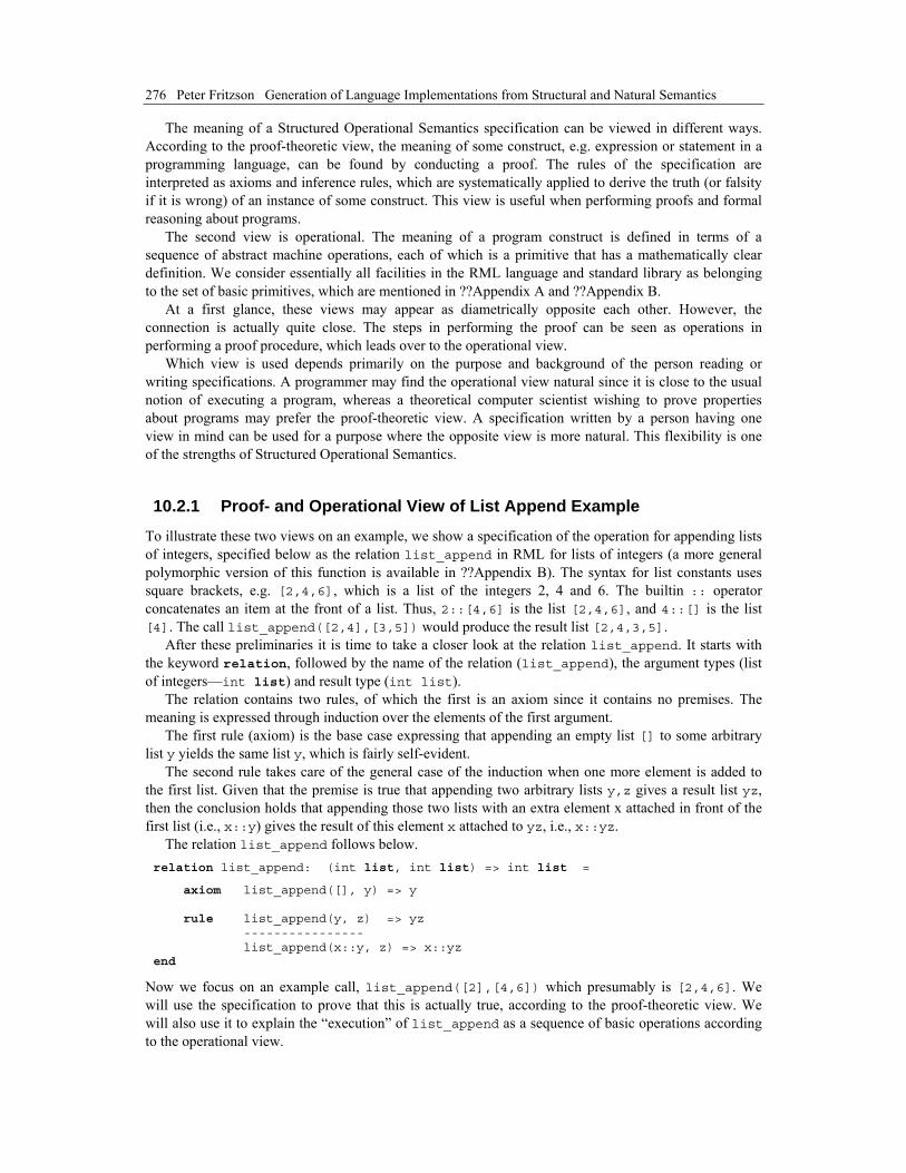
276 Peter Fritzson Generation of Language Implementations from Structural and Natural Semantics
The meaning of a Structured Operational Semantics specification can be viewed in different ways. According to the proof-theoretic view, the meaning of some construct, e.g. expression or statement in a programming language, can be found by conducting a proof. The rules of the specification are interpreted as axioms and inference rules, which are systematically applied to derive the truth (or falsity if it is wrong) of an instance of some construct. This view is useful when performing proofs and formal reasoning about programs.
The second view is operational. The meaning of a program construct is defined in terms of a sequence of abstract machine operations, each of which is a primitive that has a mathematically clear definition. We consider essentially all facilities in the RML language and standard library as belonging to the set of basic primitives, which are mentioned in ??Appendix A and ??Appendix B.
At a first glance, these views may appear as diametrically opposite each other. However, the connection is actually quite close. The steps in performing the proof can be seen as operations in performing a proof procedure, which leads over to the operational view.
Which view is used depends primarily on the purpose and background of the person reading or writing specifications. A programmer may find the operational view natural since it is close to the usual notion of executing a program, whereas a theoretical computer scientist wishing to prove properties about programs may prefer the proof-theoretic view. A specification written by a person having one view in mind can be used for a purpose where the opposite view is more natural. This flexibility is one of the strengths of Structured Operational Semantics.
10.2.1 Proof- and Operational View of List Append Example
To illustrate these two views on an example, we show a specification of the operation for appending lists of integers, specified below as the relation list_append in RML for lists of integers (a more general polymorphic version of this function is available in ??Appendix B). The syntax for list constants uses square brackets, e.g. [2,4,6], which is a list of the integers 2, 4 and 6. The builtin :: operator concatenates an item at the front of a list. Thus, 2::[4,6] is the list [2,4,6], and 4::[] is the list [4]. The call list_append([2,4],[3,5]) would produce the result list [2,4,3,5].
After these preliminaries it is time to take a closer look at the relation list_append. It starts with the keyword relation, followed by the name of the relation (list_append), the argument types (list of integers—int list) and result type (int list).
The relation contains two rules, of which the first is an axiom since it contains no premises. The meaning is expressed through induction over the elements of the first argument.
The first rule (axiom) is the base case expressing that appending an empty list [] to some arbitrary list y yields the same list y, which is fairly self-evident.
The second rule takes care of the general case of the induction when one more element is added to the first list. Given that the premise is true that appending two arbitrary lists y,z gives a result list yz, then the conclusion holds that appending those two lists with an extra element x attached in front of the first list (i.e., x::y) gives the result of this element x attached to yz, i.e., x::yz.
The relation list_append follows below. relation list_append: (int list, int list) => int list =
axiom list_append([], y) => y rule list_append(y, z) => yz ---------------- list_append(x::y, z) => x::yz end
Now we focus on an example call, list_append([2],[4,6]) which presumably is [2,4,6]. We will use the specification to prove that this is actually true, according to the proof-theoretic view. We will also use it to explain the “execution” of list_append as a sequence of basic operations according to the operational view.

Chapter 10 Structured Operational Semantics and Properties of RML 277
Starting with the operational view, which is well-known for programmers, the “execution” of list_append proceeds as follows: The call list_append([2],[4,6]) is matched against the left side of the conclusion proposition for each rule in top-down order. Thus, the term list_append([2],[4,6]) is first matched against list_append([],y), which fails since the first argument—the list [2]—is not equal to []. The second argument is no problem since it will match if y is bound to [4,6]. However, a complete match is required for the rule to succeed. Thus, the first rule (the axiom) fails.
Next, the second rule is tried, for which the term list_append([2],[4,6]) is matched against the pattern list_append(x::y,z). The list_append head of the term matches, of course. The first argument matches if [2] and x::y can be made to match, which is indeed possible if x is bound to 2 and y to [], giving 2::[] which is identical to [2] (just different syntax). The second argument ([4,6]) matches if z is bound to [4,6]. Thus, the second rule matches with x bound to 2, y to [] and z to [4,6]. The next step is to evaluate the premise of the second rule: list_append(y,z)=>yz. With the above bindings of y and z this becomes list_append([], [4,6]), which becomes [4,6] (i.e., yz) after recursively calling list_append and matching against the first rule (axiom). This ends the recursion since the axiom contains no recursive invocation of list_append. Finally, the result of the conclusion becomes x::yz which is 2::[4,6]—identical to [2,4,6], the expected final result.
In the proof-theoretic view, we want to prove that there is a value v such that list_append([2],[4,6]) => v, with v equal to [2,4,6]. The proof is performed by repeatedly applying the axioms and inference rules of the specification. First we instantiate the second rule, giving:
list_append([],[4,6]) => yz —————————————————— (9.4)?? list_append(2::[],[4,6]) => 2::yz
Next, we must prove the premise list_append([],[4,6]=>yz. The proof tree is therefore extended by instantiating the first rule (the axiom) and replacing yz with [4,6], giving:
true —————————————————— list_append([],[4,6]) => [4,6] ———————————————————— (9.5)?? list_append(2::[],[4,6]) => 2 :: [4,6]
Since the used axiom has no visible premises, we put true (which always is true) as its premise. The proof is now complete since no other propositions need to be proven. By using the syntactic and semantic equivalence of 2::[4,6] and [2,4,6], we finally obtain the desired proof:
true —————————————————— list_append([],[4,6]) => [4,6] ———————————————————— (9.6)?? list_append(2::[],[4,6]) => [2,4,6]
As seen in this example, proof trees are constructed upside down, with the conclusion at the bottom, i.e., at the top of a tree turned upside down. This proof tree is somewhat degenerate, in that it has only one branch. Typically, most inference rules have several premises, giving rise to many branches.

278 Peter Fritzson Generation of Language Implementations from Structural and Natural Semantics
10.3 ??Some RML Issues
10.3.1 Determinism versus Nondeterminism
We earlier remarked that in Structured Operational Semantics, specifications are generally determinate, i.e., for any proposition at most one inference rule in the called relation can be applicable in a proof of that proposition. (*?? fill in some stuff)
(*?? Give an example where non-determinism would be appropriate in a specification, and how it could be reformulated in a deterministic way)
10.3.2 Variable Bindings
We have already explained that variable bindings are created in RML during pattern matching. Local variable bindings can also be introduced directly through the let syntax used in the following example, where a local variable x is introduced and bound to the value 55: let x = 55
10.3.3 Unknowns and Logical Variables
(??Should this section be removed because of RML V2?)
10.3.4 Representing Symbols
Many symbolic languages, especially in the Lisp tradition, represent symbols by unique integers— usually called “atoms”—obtained by hashing the symbol string at symbol creation time. This has the advantage that equality of two symbols can be tested with a single integer comparison, and that the symbol contents—the string—is only stored once.
However, in RML, and also in languages like Standard ML, symbols are usually represented by string values. The disadvantage is that a few comparison instructions (usually just a test on the header and a few byte- or word comparisons) are needed to implement string comparison, instead of just a single pointer comparison. However, there is also an advantage. The representation of string values is known at compile time, which can be used by a compiler to implement pattern matching on strings rather efficiently. Pattern matching is also a very common operation in RML and Standard ML. On the other hand, atoms are not created until run-time (by hashing), which then causes pattern matching and case statements to be implemented as linear sequences of tests. If desired, atoms could however easily be added to RML by external C routines.
10.4 Performance of Generated Implementations The performance of translator modules in C generated from RML specifications is quite good— comparable to handwritten implementations in Pascal or C. For example, the compiler for the Pascal-like Petrol language runs 30% faster than a hand-written compiler for a subset of Petrol (implemented in Pascal) on the same test example. A generated interpreter for a small call-by-name functional language (called Mini-Freja) is several orders of magnitude faster than a similar interpreter generated by the Centaur/TYPOL system.
(?? Insert performance table)

Chapter 10 Structured Operational Semantics and Properties of RML 279
(BRK)


281
Appendix A – RML Language Constructs This appendix contains a short overview of the syntax and semantics of all constructs in the RML specification language. For a complete description, including a Structured Operational Semantics specification of RML itself, see Appendix ?? of Mikael Petterson’s Ph.D. thesis [ref??].
A.1 RML concrete syntax Below is brief rundown of the RML concrete syntax. Keywords and special symbols (eg, *, &, =) are shown in bold letters, other tokens are shown in capital letters. Some constructs are explained further with aid of simple examples in curly brackets following the syntax production. Module : Interface Dec Interface : module Modid : Spec end Dec : with STRINGCONST { with "file.rml" } | type Typbind { type val = int } | datatype Datbind Withbind { datatype Complex = COMP of int *int } | relation Relbind | val Var = Exp { val zero = COMP(0,0) } | Dec Dec Spec : with STRINGCONST | abstype Tyvarseq Tycon { abstype int } | type Typbind | datatype Datbind withbind | relation Var : Tyseq => Tyseq { relation add_comp: (Complex, Complex) => Complex } | val Var : Ty { val zero : Complex } | Spec Spec RelBind : Var = Clause end | Var : Tyseq => Tyseq = Clause end | Relbind and Relbind Withbind : | withtype Typbind Typbind : Tyvarseq Tycon = Ty { ’a list = nil } | Typbind and Typbind Datbind : Tyvarseq Tycon = Conbind { ’a list = cons of ’a * ’a list } | Datbind and Datbind Conbind : Con { NONE } | Con of Tys { SOME of ’a } | Conbind | Conbind { true | false }

282 Peter Fritzson Generation of Language Implementations from Structural and Natural Semantics
Clause : rule Goalopt -- Var Patseqopt Expseqopt { rule z = zero --------- is_zero z => true } | axiom Var Patseqopt Expseqopt { axiom is_zero COMP(0, 0) => true } | Clause Clause RetExpseqopt : | => Expseqopt { => true } Goal : Longvar Expseqopt RetPatseqopt { Math.add_comp(z) => r} | Var = Exp { z1 = z2 } | exists Var { exists a } | not Goal { not is_zero } | Goal & Goal { not is_zero z & is_zero z } | ( Goal ) { (is_zero z ) } Goalopt : | Goal RetPatseqopt : | => Patseqopt { => (_, true) } Patseqopt : | Patseq { (true, false, _) } Expseqopt : | Expseq { (zero, true) } Expseq : Exp | ( Explist ) { ((zero, true)) } Exp : Lit { "astring" } | [ Explist ] { [1, 2, 3] } | Longcon { Math.Complex } | Longvar { Math.zero } | Longcon Expseq { Math.Complex(4, 2) } | ( Explist ) { (1, 2) } | Exp :: Exp { first::rest } Explist : | Explist1 Explist1 : Exp | Explist1 , Exp Patseq : Pat

Appendix A – RML Language Constructs 283
{ _ } | ( Patlist ) { (_, "foo", #"a", true) } Pat : _ { _ } | Lit | [ Patlist ] | Longcon | Var | Longcon Patseq { Math.COMP(_, _) } | ( Patlist ) { (_, true, "abc", #"A") } | Pat :: Pat { _::rest } | Var as Pat { z as COMP(_,_) } Patlist1 : Pat | Patlist1 , Pat Patlist : | Patlist1 TySeq : ( ) | Ty | ( Tylist ) Tylist : Ty | Tylist , Ty Ty : Tyvar { ’a } | Tyseqopt Longtycon { (int, int) Math.COMP} | Tys { int * char * string } | Tyseq => Tyseq { (Complex, Complex) => Complex } | ( Ty ) Tys : Ty * Ty { int * int } | Tys * Ty { int * int * int } Tyseqopt : | Tyseq Tyvarlist : Tyvar { ’a } | Tyvarlist , Tyvar { ’a, ’b } Tyvarseq : | Tyvar | ( Tyvarlist ) Lit : CHARACTERCONST { #"A" } | INTCONST { 1 }
284 Peter Fritzson Generation of Language Implementations from Structural and Natural Semantics
| REALCONST { 3.14 } | STRINGCONST { "abcde" } Longvar : Modidopt Var { Math.zero } Longcon : Modidopt Con { Math.COMP } Longtycon : Modidopt Tycon { Math.Complex } Modidopt : | Modid . Modid : IDENT Var : IDENT Con : IDENT Tycon : IDENT
(BRK)

285
Appendix B – Predefined RML primitives This appendix contains a number of basic primitives, for which the semantics are assumed to be known or having a mathematical definition. It is based on Appendix ?? of [**RefMikaelsthesis]. The definitions are packaged in a standard RML module, called rml, as can be seen below. Some of these primitives are themselves formally defined in RML in this appendix, although more efficient implementations are provided by the RML runtime system. First the type signatures of all predefined primitives are presented. Then the semantics of some primitives are explained or defined in RML.
B.1 Interface to the Standard RML Module The following subsections present type signatures for all builtin RML primitives. First comes the module header for the rml module: module rml:
B.1.1 Predefined Types and Type Constructors abstype char abstype int abstype real abstype string abstype 'a vector datatype bool = false | true datatype 'a list = nil | cons of 'a * 'a list datatype 'a option = NONE | SOME of 'a
B.1.2 Boolean Operations relation bool_and: (bool,bool) => bool relation bool_or: (bool,bool) => bool relation bool_not: bool => bool
B.1.3 Integer Operations relation int_add: (int,int) => int relation int_sub: (int,int) => int relation int_mul: (int,int) => int relation int_div: (int,int) => int relation int_mod: (int,int) => int relation int_abs: int => int relation int_neg: int => int relation int_max: (int,int) => int relation int_min: (int,int) => int relation int_lt: (int,int) => bool relation int_le: (int,int) => bool relation int_eq: (int,int) => bool relation int_ne: (int,int) => bool relation int_ge: (int,int) => bool relation int_gt: (int,int) => bool relation int_real: int => real relation int_string: int => string
Some of the builtin integer relations are also available as operators according to the following table: int_add +

286 Peter Fritzson Generation of Language Implementations from Structural and Natural Semantics
int_sub - int_neg - int_mul * int_div / int_mod % int_eq == int_ne != int_ge >= int_gt > int_le <= int_lt >
B.1.4 Real number operations relation real_add: (real,real) => real relation real_sub: (real,real) => real relation real_mul: (real,real) => real relation real_div: (real,real) => real relation real_mod: (real,real) => real relation real_abs: real => real relation real_neg: real => real relation real_cos: real => real relation real_sin: real => real relation real_atan: real => real relation real_exp: real => real relation real_ln: real => real relation real_floor: real => real relation real_int: real => int relation real_pow: (real,real) => real relation real_sqrt: real => real relation real_max: (real,real) => real relation real_min: (real,real) => real relation real_lt: (real,real) => bool relation real_le: (real,real) => bool relation real_eq: (real,real) => bool relation real_ne: (real,real) => bool relation real_ge: (real,real) => bool relation real_gt: (real,real) => bool
Some of the builtin real relations are also available as operators according to the following table: real_add +. real_sub -. real_neg -. real_mul *. real_div /. real_mod %. real_pow ^. real_eq ==. real_ne !=. real_ge >=. real_gt >. real_le <=. real_lt >.
B.1.5 Character Conversion Operations relation char_int: char => int relation int_char: int => char
B.1.6 String Operations relation string_int: string => int relation string_list: string => char list

Appendix B – Predefined RML primitives 287
relation list_string: char list => string relation string_length: string => int relation string_nth: (string,int) => char relation string_append: (string,string) => string
B.1.7 List operations relation list_append: ('a list,'a list) => 'a list relation list_reverse: 'a list => 'a list relation list_length: 'a list => int relation list_member: ('a,'a list) => bool relation list_nth: ('a list, int) => 'a relation list_delete: ('a list, int) => 'a list
B.1.8 Vector operations relation vector_length: 'a vector => int relation vector_nth: ('a vector, int) => 'a relation vector_list: 'a vector => 'a list relation list_vector: 'a list => 'a vector
B.1.9 Miscellaneous operations relation clock: () => real relation isvar: 'a => bool relation print: 'a => () relation tick: () => int end (* of interface section of the rml module *)
B.2 Builtin Primitive Functions and Predicates In the following we provide approximate or exact descriptions of the builtin RML primitive functions and predicates.
• clock (?? missing description) • isvar (?? missing description) • print (?? missing description) • tick (?? missing description)
The following operations only apply to primitive RML values, which can be either a character c, an integer i, a real r, a string str, a list lst, a vector vec, or an unbound location.
• int_add(i1,i2) = i1 + i2 if the result can be represented by the implementation, otherwise the operation fails.
• int_sub(i1,i2) = i1 – i2 if the result can be represented by the implementation, otherwise the operation fails.
• int_mul(i1,i2) = i1 × i2 if the result can be represented by the implementation, otherwise the operation fails.
• int_div(i1,i2) returns the integer quotient of i1 and i2 if i2 ≠ 0 and the result can be represented by the implementation, otherwise the operation fails.
• int_mod(i1,i2) returns the integer remainder of i1 and i2 if i2 ≠ 0 and the result can be represented by the implementation, otherwise the operation fails.
• int_abs(i) returns the absolute value of i if the result can be represented by the implementation, otherwise the operation fails.
• int_neg(i) returns –i if the result can be represented by the implementation, otherwise the • operation fails. • int_max(i1,i2) = i1 if i1 ≥ i2, otherwise i2.

288 Peter Fritzson Generation of Language Implementations from Structural and Natural Semantics
• int_min(i1,i2) = i1 if i1 ≤ i2, otherwise i2. • int_lt(i1,i2) = true if i1 < i2, otherwise false. • int_le(i1,i2) = true if i1 ≤ i2, otherwise false. • int_eq(i1,i2) = true if i1 = i2, otherwise false. • int_ne(i1,i2) = true if i1 ≠ i2, otherwise false. • int_ge(i1,i2) = true if i1 ≥ i2, otherwise false. • int_gt(i1,i2) = true if i1 > i2, otherwise false. • int_real(i) = r where r is the corresponding real value equal to i. • int_string(i) returns a textual representation of i, as a string. • real_add(r1,r2) = r1 + r2. • real_sub(r1,r2) = r1 – r2. • real_mul(r1,r2) = r1 × r2. • real_div(r1,r2) = r1 / r2. • real_mod(r1,r2) = returns the remainder of r1 / r2. This is the value r1 – i × r2, for some
integer i such that the result has the same sign as r1 and magnitude less than the magnitude of r2. If r2 = 0, the operation fails.
• real_abs(r) returns the absolute value of r. • real_neg(r) = –r. • real_cos(r) returns the cosine of r (measured in radians). • real_sin(r) returns the sine of r (measured in radians). • real_atan(r) returns the arc tangent of r. • real_exp(r) returns re . • real_ln(r) returns ln(r). • real_floor(r) returns the largest integer (as a real value) not greater than r. • real_int(r) discards the fractional part of r and returns the integral part as an integer; fails if
this value cannot be represented by the implementation. • real_pow(r1,r2) = 21rr ; fails if this cannot be computed. • real_sqrt(r) = r ; fails if r < 0. • real_max(r1,r2) = r1 if r1 ≥ r2, otherwise r2. • real_min(r1,r2) = r1 if r1 ≤ r2, otherwise r2. • real_lt(r1,r2) = true if r1 < r2, otherwise false. • real_le(r1,r2) = true if r1 ≤ r2, otherwise false. • real_eq(r1,r2) = true if r1 = r2, otherwise false. • real_ne(r1,r2) = true if r1 ≠ r2, otherwise false. • real_ge(r1,r2) = true if r1 ≥ r2, otherwise false. • real_gt(r1,r2) = true if r1 > r2, otherwise false.
• string_int(str) = i if the string str has the lexical structure of an integer constant and i is the value associated with that constant. Otherwise the operation fails.
B.3 Derived Functions for Booleans, Strings, Lists and Vectors The behavior of certain standard RML relations (really functions) can be defined in RML itself. These include the boolean, list, character and vector operations, and some string operations. Implementations are supposed to supply equivalent, but usually more efficient, versions of these functions.
Even though the vector and string types can be defined in terms of lists, the implementations of the builtin RML relations vector_length, vector_nth, string_length, and string_nth are assumed to execute in constant time.
B.3.1 Boolean Operations relation bool_and: (bool,bool) => bool =

Appendix B – Predefined RML primitives 289
axiom bool_and(true, true) => true axiom bool_and(true, false) => false axiom bool_and(false, true) => false axiom bool_and(false, false) => false end relation bool_or: (bool,bool) => bool = axiom bool_or(false, false) => false axiom bool_or(false, true) => true axiom bool_or(true, false) => true axiom bool_or(true, true) => true end relation bool_not: bool => bool = axiom bool_not false => true axiom bool_not true => false end
B.3.2 List Operations These definitions give the semantics of the list operations, not the actual implementation. relation list_append: ('a list, 'a list) => 'a list =
axiom list_append([], y) => y rule list_append(y, z) => w ---------------- list_append(x::y, z) => x::w end relation list_reverse: 'a list => 'a list = axiom list_reverse([]) => [] rule list_reverse(y) => revy & list_append(revy, [x]) => z ---------------- list_reverse(x::y) => z end relation list_length: 'a list => int = axiom list_length([]) => 0 rule list_length(y) => leny & int_add(1,leny) => z ---------------- list_length(_::y) => z end relation list_member: ('a, 'a list) => bool = axiom list_member(_, []) => false rule x = y ---------------- list_member(x, y::ys) => true rule not x = y & list_member(x, ys) => z ---------------- list_member(x, y::ys) => z end relation list_nth: ('a list, int) => 'a =
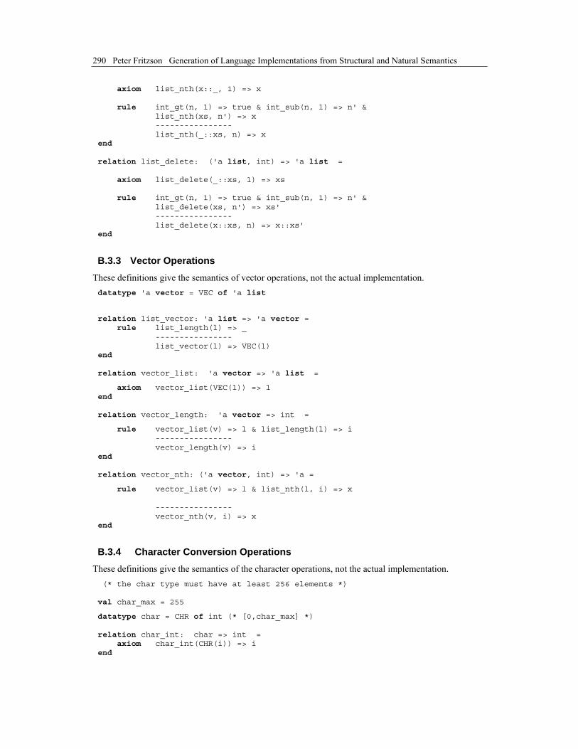
290 Peter Fritzson Generation of Language Implementations from Structural and Natural Semantics
axiom list_nth(x::_, 1) => x rule int_gt(n, 1) => true & int_sub(n, 1) => n' & list_nth(xs, n') => x ---------------- list_nth(_::xs, n) => x end relation list_delete: ('a list, int) => 'a list = axiom list_delete(_::xs, 1) => xs rule int_gt(n, 1) => true & int_sub(n, 1) => n' & list_delete(xs, n') => xs' ---------------- list_delete(x::xs, n) => x::xs' end
B.3.3 Vector Operations These definitions give the semantics of vector operations, not the actual implementation. datatype 'a vector = VEC of 'a list
relation list_vector: 'a list => 'a vector = rule list_length(l) => _ ---------------- list_vector(l) => VEC(l) end relation vector_list: 'a vector => 'a list =
axiom vector_list(VEC(l)) => l end relation vector_length: 'a vector => int =
rule vector_list(v) => l & list_length(l) => i ---------------- vector_length(v) => i end relation vector_nth: ('a vector, int) => 'a =
rule vector_list(v) => l & list_nth(l, i) => x ---------------- vector_nth(v, i) => x end
B.3.4 Character Conversion Operations These definitions give the semantics of the character operations, not the actual implementation. (* the char type must have at least 256 elements *) val char_max = 255
datatype char = CHR of int (* [0,char_max] *) relation char_int: char => int = axiom char_int(CHR(i)) => i end

Appendix B – Predefined RML primitives 291
relation int_char: int => char =
rule int_ge(i,0) => true & int_le(i,char_max) => true ---------------- int_char(i) => CHR(i) end
B.3.5 String Operations These definitions give the semantics of the string operations, not the actual implementation. datatype string = STR of char vector relation list_string: char list => string =
rule list_vector(l) => v ---------------- list_string(l) => STR(v) end relation string_list: string => char list =
rule vector_list(v) => l ---------------- string_list(STR(v)) => l end relation string_length: string => int =
rule vector_length(v) => i ---------------- string_length(STR(v)) => i end relation string_nth: (string,int) => char =
rule vector_nth(v, i) => c ---------------- string_nth(STR(v), i) => c end relation string_append: (string,string) => string =
rule string_list(s1) => l1 & string_list(s2) => l2 & list_append(l1, l2) => l3 & list_string(l3) => s3 ---------------- string_append(s1, s2) => s3 end


293
Index Error! No index entries found.