Methodology Report

FHWA

TOPR 33-01-18005:

Developing a Statistically Valid and Practical Method

to Compute Bus and Truck Occupancy Data

Technical and Program Support for Highway Policy Analysis

May 29, 2019

Notice This document is disseminated under the sponsorship of the United States Department of

Transportation in the interest of information exchange. The United States Government assumes

no liability for its contents or use thereof. This report does not constitute a standard,

specification, or regulation.

The United States Government does not endorse products or manufacturers. Trade and

manufacturers’ names appear in this report only because they are considered essential to the

object of the document.

Quality Assurance Statement

The Federal Highway Administration (FHWA) provides high-quality information to serve

Government, industry, and the public in a manner that promotes public understanding. Standards

and policies are used to ensure and maximize the quality, objectivity, utility, and integrity of its

information. FHWA periodically reviews quality issues and adjusts its programs and processes to

ensure continuous quality improvement.

Technical Report Documentation Page

1. Report No.

PL-19-048

2. Government Accession No. 3. Recipient's Catalog No.

4. Title and Subtitle

Developing a Statistically Valid and Practical Method to Compute Bus and Truck

Occupancy Data

5. Report Date

6. Performing Organization Code

8. Performing Organization Report No. 7. Author(s)

Yinhai Wang, Roger Mingo, Jerome M. Lutin, Wenbo Zhu, and Meixin Zhu

9. Performing Organization Name and Address

University of Washington

More Hall 133B

Box 352700

Seattle, WA 98195

10. Work Unit No. (TRAIS)

11. Contract or Grant No.

DTFH61-13-D-00021/693JJ318F000037

13. Type of Report and Period Covered

12. Sponsoring Agency Name and Address

Federal Highway Administration

Office of Highway Policy Information

1200 New Jersey Avenue SE

Washington, DC 20590 14. Sponsoring Agency Code

15. Supplementary Notes

The project was managed by Task Managers for the Federal Highway Administration, Wenjing Pu and Daniel Jenkins, who provided

technical directions.

16. Abstract

This project aims to assist the Federal Highway Administration (FHWA) in providing data to states and metropolitan areas in

accordance with Title 23 of the US Code of Federal Regulations, Part 490 National Performance Management Measures. The specific

task is to provide and implement a statistically valid and practical method to estimate bus and truck occupancy rates for each

urbanized area (UZA) as defined by the U.S. Census Bureau, each state, and the District of Columbia (DC). All fifty states, DC, and

183 UZA’s with a population higher than 200,000 are included in this project.

Bus occupancies were estimated separately for each of three categories: transit bus, school bus, and motorcoach. Average total bus

occupancy was estimated by aggregating the average vehicle occupancies (AVO) for the above three categories weighted by annual

vehicle miles traveled (VMT). Specifically, the Federal Transit Administration (FTA) National Transit Database (NTD) was used to

calculate transit bus occupancy; “U.S. State by State Transportation Statistics 2015-16,” reported by SchoolBusFleet.com were used to

calculate average school bus occupancy for each state; and data provided by the Port Authority of New York and New Jersey

(PANYNJ) for the Port Authority Bus Terminal (PABT) in New York City, the largest bus terminal in the US, were used to calculate

motorcoach occupancy rates. For trucks, an overall average truck occupancy rate was calculated for all truck types based on National

Highway Traffic Safety Administration (NHTSA) Trucks in Fatal Accidents (TIFA) data.

Results show that the mean state-level bus occupancy rate is 20.29, with a standard deviation of 5.24; and the mean state-level truck

occupancy rate is 1.19, with a standard deviation of 0.07. Recommendations for future work include (1) work with providers of the

various relevant data sources to ensure access to regularly updated new data; (2) initiate a training program for the software code to

ensure the results can be easily updated in the future; and (3) make further use of the proposed alternative methods to validate results.

17. Key Words Bus Occupancy, Truck Occupancy, Transit, School Bus,

Motorcoach, Urbanized Area

18. Distribution Statement No restrictions. This document is available to the public

19. Security Classif. (of this report)

Unclassified

20. Security Classif. (of this page)

Unclassified

21. No. of Pages

35

22. Price

Form DOT F 1700.7 (8-72) Reproduction of completed page authorized

Contents

General Background ..................................................................................................................... 1

PROBLEM STATEMENT ..................................................................................................................................................... 1

GOALS AND SCOPE OF WORK ............................................................................................................................................ 1

Methodology .................................................................................................................................. 5

DEVELOPING BUS OCCUPANCY FACTORS ............................................................................................................................. 5

Methodology Framework ...................................................................................................................................... 5

Methodology: Transit Bus ..................................................................................................................................... 6

Methodology: School Bus .................................................................................................................................... 13

Methodology: Motorcoach (Private Bus) ............................................................................................................ 22

DEVELOPING TRUCK OCCUPANCY FACTORS ....................................................................................................................... 28

Methodology Framework .................................................................................................................................... 28

Methodology: Truck ............................................................................................................................................ 28

TESTING RESULT ........................................................................................................................................................... 32

References .................................................................................................................................... 34

Page 1

General Background

Problem Statement

Many urban areas have introduced varieties of transportation management strategies which are

designed to reduce the number of vehicles on the road. Some of these methods are aiming to

encourage more high-occupancy-vehicle (HOVs) on the road to avoid severe congestion. Thus,

monitoring and estimating average vehicle occupancy (AVO) has become a key prerequisite

before implementing these strategies. Often, AVO rates are acquired via road-side video-

recording and carousel methods. Heidtman et al. (1997) set up an observation team along the

side of the roadway to count the passengers in the vehicles passing by, and they concluded that

the method was most effective for collecting data for corridors and roadways of low functional

classification, but less effective on multilane freeways. Hao et al. (2011) developed an imaging

technique to make the occupants more visible in the vehicle, by use of infrared, while

simultaneously using a video recording system. A study of vehicle occupancy conducted in

Arizona used the carousel method as a supplement to roadside observations for AVO estimation,

and applied a carousel method usually that used more than one vehicle with several observers in

the traffic stream to observe occupants in other vehicles (MAG, 2013).

In addition to technical methodologies, researchers have also used survey and crash datasets to

estimate vehicle occupancy. Gan et al. (2005) developed a user-friendly software system which

could be used to estimate occupancy rates in Florida from multiple years of crash data; the

system also included a stand-alone GIS interface to facilitate the selection of geographic features

and display of occupancy rate estimates. Gan et al. (2008) also carried out a thorough AVO

estimation study using existing traffic crash data co-modeled with other variables such as district,

county, hour, week etc. However, in their paper, they admitted that the results are highly

susceptible to potential bias resulting from issues related to traffic crash reports. Jung et al.

(2010) provided a detailed process for estimating AVOs at the individual location, facility type,

and county levels, along with a detailed sampling process designed to select data collection

locations and dates on different facility types.

While aforementioned studies have implemented AVO estimation methods that have proven to

work well, they are limited in their scope and often focused on a geographic area no larger than a

state. Additionally, methods that involve manual counts are too time and resource intensive to be

used to estimate AVO of each urban area nationwide. More importantly, most of the methods

mentioned does not include a special consideration for AVO rates of buses and trucks. As such,

methods are needed that can be applied nationally and only rely on data that are easily available

nationwide, and are updated regularly. For this project, in order to estimate vehicle occupancy

for urbanized areas nationwide, a combination of national-wide, local, and survey data will be

used for large-scale sampling and modeling work.

Goals and Scope of Work

The goal of this task order is to provide and implement a statistically valid and practical method

to estimate 1) bus occupancy rate for each of the urbanized areas as defined by the U.S. Census

Bureau and each of the states and the District of Columbia and 2) truck occupancy rate for each

of the urbanized areas as defined by the U.S. Census Bureau and each of the states and the

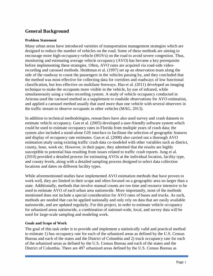
District of Columbia. There are 497 urbanized areas defined by the U.S. Census Bureau as

Page 2

shown in Figure 1. Note that this project will only include the urbanized area with a population

higher than 200,000. After filtering the urbanized area based on the population information

obtained from the U.S. Census Bureau (U.S. Census Bureau, 2012), 183 urbanized areas are

considered in this project. Table 1 summarizes top 20 urbanized areas in terms of population. To

map different data into the urbanized areas, the U.S. Census Bureau website also provides a set

of files that contains the relationships between the urbanized areas and other geospatial regions

(e.g., county, city, and zip code) (U.S. Census Bureau, 2010).

The tasks are to develop statistically valid and practical methods to estimate a) bus occupancy

rate each of the urbanized areas as defined by the U.S. Census Bureau and each of the states and

the District of Columbia and b) truck occupancy rate for each of the urbanized areas as defined

by the U.S. Census Bureau and each of the states and the District of Columbia.

Figure 1. Urbanized areas in the United States. Source:

https://en.wikipedia.org/wiki/United_States_urban_area#/media/File:USA-Urban-Areas.svg.

Page 3

Table 1. Top 20 Urbanized Areas in US Urban

Code

Name State Population Land Area

(mi2)

Population

Density

63217 New York--Newark, NY--NJ--CT NY 12,191,715 1563.15 7799.5

51445 Los Angeles--Long Beach--Anaheim, CA CA 12,150,996 1736.02 6999.3

16264 Chicago, IL--IN IL 8,018,716 2122.25 3778.4

63217 New York--Newark, NY--NJ--CT NJ 6,159,466 1886.99 3264.2

56602 Miami, FL FL 5,502,379 1238.61 4442.4

22042 Dallas--Fort Worth--Arlington, TX TX 5,121,892 1779.13 2878.9

40429 Houston, TX TX 4,944,332 1660.02 2978.5

3817 Atlanta, GA GA 4,515,419 2645.35 1706.9

9271 Boston, MA--NH--RI MA 4,087,709 1750.57 2335.1

69076 Philadelphia, PA--NJ--DE--MD PA 3,760,387 1245.92 3018.2

23824 Detroit, MI MI 3,734,090 1337.16 2792.5

69184 Phoenix--Mesa, AZ AZ 3,629,114 1146.57 3165.2

78904 San Francisco--Oakland, CA CA 3,281,212 523.62 6266.4

80389 Seattle, WA WA 3,059,393 1010.31 3028.2

78661 San Diego, CA CA 2,956,746 732.41 4037

57628 Minneapolis--St. Paul, MN--WI MN 2,650,614 1021.31 2595.3

86599 Tampa--St. Petersburg, FL FL 2,441,770 956.99 2551.5

23527 Denver--Aurora, CO CO 2,374,203 667.95 3554.4

92242 Washington, DC--VA--MD VA 2,235,884 696.16 3211.7

4843 Baltimore, MD MD 2,203,663 717.04 3073.3

The term of “statistically valid” means that the information generated from any underlying data

used in the estimation should be representative of the entire population with an 85% confidence

interval. The term of “practical” means that the method is not relying on a new survey activity,

doesn’t cost more than $250,000 to implement the methods for all urbanized areas and states on

an annual basis, and can be completed within 6 months after the end of year. Here, bus is defined

as Class 4 vehicles in FHWA’s 13 Vehicle Category Classification. According to FHWA’s 13

Vehicle Category Classification, trucks are defined as Class 5 through Class 13 vehicles, but this

project specifically considers Class 6-13 (as requested by the TOPR, see Figure 2) vehicles when

estimating average truck occupancy. For bus occupancy rates, factors will cover both the public

and private charters, transit, school, tourism and long-distance service buses.

Page 4

Figure 2. Definition of bus and truck based on FHWA vehicle classification. Source:

https://www.agroclasi.com/freight-class-chart-pdf/using-truck-fleet-data-in-combination-with-

other-sources-for-fhwa_classification_chart_/.

Page 5

Methodology

Developing Bus Occupancy Factors

Methodology Framework

Generally, buses defined as Class 4 vehicles in FHWA’s 13 Vehicle Category Classification can

be subdivided into three categories: (1) transit bus (metro bus); (2) school bus; and (3)

motorcoach. Total average bus occupancy can be estimated by aggregating the average vehicle

occupancies (AVO) for the above three subgroups as shown below:

𝐴𝑉𝑂𝐵𝑢𝑠

=𝐴𝑉𝑂𝑇𝑟𝑎𝑛𝑠𝑖𝑡 × 𝑉𝑀𝑇𝑇𝑟𝑎𝑛𝑠𝑖𝑡 + 𝐴𝑉𝑂𝑆𝑐ℎ𝑜𝑜𝑙 × 𝑉𝑀𝑇𝑆𝑐ℎ𝑜𝑜𝑙 + 𝐴𝑉𝑂𝑀𝑜𝑡𝑜𝑟𝑐𝑜𝑎𝑐ℎ × 𝑉𝑀𝑇𝑀𝑜𝑡𝑜𝑟𝑐𝑜𝑎𝑐ℎ

𝑉𝑀𝑇𝑇𝑟𝑎𝑛𝑠𝑖𝑡 + 𝑉𝑀𝑇𝑆𝑐ℎ𝑜𝑜𝑙 + 𝑉𝑀𝑇𝑀𝑜𝑡𝑜𝑟𝑐𝑜𝑎𝑐ℎ

where 𝐴𝑉𝑂 =Average Vehicle Occupancy; VMT=Annual Vehicle Miles Traveled. It is

necessary to develop the bus occupancy factors based on the above three subgroups because their

AVOs differ significantly. Our methodology estimates the AVOs for transit bus, school bus, and

motorcoach independently based on multi-source datasets from state and urbanized area levels,

and then aggregates them based on their proportion of total bus VMT. The VMT for each bus

category can be calculated based on their average VMT (national level) and the vehicle count

data from the Polk dataset which contains detailed vehicle registration information (Polk City

Directory, 2018) by using the following equations:

𝑉𝑀𝑇𝑇𝑟𝑎𝑛𝑠𝑖𝑡 = 𝐴𝑣𝑒𝑟𝑎𝑔𝑒 𝑉𝑀𝑇𝑇𝑟𝑎𝑛𝑠𝑖𝑡 × 𝑉𝑒ℎ𝑖𝑐𝑙𝑒 𝐶𝑜𝑢𝑛𝑡𝑇𝑟𝑎𝑛𝑠𝑖𝑡

𝑉𝑀𝑇𝑆𝑐ℎ𝑜𝑜𝑙 = 𝐴𝑣𝑒𝑟𝑎𝑔𝑒 𝑉𝑀𝑇𝑆𝑐ℎ𝑜𝑜𝑙 × 𝑉𝑒ℎ𝑖𝑐𝑙𝑒 𝐶𝑜𝑢𝑛𝑡𝑆𝑐ℎ𝑜𝑜𝑙

𝑉𝑀𝑇𝑀𝑜𝑡𝑜𝑟𝑐𝑜𝑎𝑐ℎ = 𝐴𝑣𝑒𝑟𝑎𝑔𝑒 𝑉𝑀𝑇𝑀𝑜𝑡𝑜𝑟𝑐𝑜𝑎𝑐ℎ × 𝑉𝑒ℎ𝑖𝑐𝑙𝑒 𝐶𝑜𝑢𝑛𝑡𝑀𝑜𝑡𝑜𝑟𝑐𝑜𝑎𝑐ℎ

where 𝐴𝑣𝑒𝑟𝑎𝑔𝑒 𝑉𝑀𝑇𝑇𝑟𝑎𝑛𝑠𝑖𝑡 = 34,053 miles per vehicle (U.S. Department of Energy, 2015);

𝐴𝑣𝑒𝑟𝑎𝑔𝑒 𝑉𝑀𝑇𝑆𝑐ℎ𝑜𝑜𝑙 = 12,000 miles per vehicle (American School Bus Council, 2015);

𝐴𝑣𝑒𝑟𝑎𝑔𝑒 𝑉𝑀𝑇𝑀𝑜𝑡𝑜𝑟𝑐𝑜𝑎𝑐ℎ = 38,385 miles per vehicle (American Bus Association, 2017). The

state-level bus count by type is shown in Figure 3.

Page 6

Figure 3. State level bus count by type.

Figure 4 illustrates the general framework of our methodology for developing bus occupancy

factors. The details about how to estimate the AVOs for transit bus, school bus, and motorcoach

will be explained in the following sections.

Figure 4. General framework for developing bus occupancy factors.

Methodology: Transit Bus

Data Sources

The primary dataset used for transit bus occupancy calculation is the Federal Transit

Administration (FTA) National Transit Database (NTD). The most recent dataset is for the year

2017. All public bus companies that receive Federal funding are required to annually report

operational and financial data to the FTA, including transit modes operated, number of vehicles

in operation, service hours, etc. Passenger and vehicle miles traveled, the two variables used in

occupancy calculation, are also included in the NTD.

Transit agencies are classified into three types of reporters, “Full Reporter”, “Reduced Reporter”,

and “Rural Reporter.” Only data from “Full Reporters” has been certified as to accuracy by each

Transit bus

（Metro bus)

School bus

Motorcoach

Bus

Average occupancy Average VMT

Average occupancy Average VMT

Average occupancy Average VMT

Vehicle count

Vehicle count

Vehicle count

Bus occupancy

Aggregation

Page 7

agency’s CEO and subjected to audit according to the FHWA requirement (FHWA, 2017). After

filtering out transit modes that are not considered in this project (e.g., rail and ferry transit), the

final dataset includes five transit modes: Commuter Bus (CB), Demand Responsive (DR), Motor

Bus (MB), Rapid Bus (Bus Rapid Transit) (RB), and Trolley Bus (TB). For these five modes, a

total of 1,051 bus transit agencies were labeled as “Full Reporters” as of 2016. Table 2 presents

the reporting rate for transit agencies of different modes. In general, NTD data shows a very high

reporting rate (i.e., around 99% across all transit modes) and it is not necessary to impute

missing data.

Table 2. Reporting Rate for Transit Agencies of Different Modes Transit Mode # of PMT/VMT Reports Total Count Report Rate

Commuter Bus (CB) 101 102 99.0%

Demand Responsive (Paratransit) (DR) 454 458 99.1%

Motor Bus (MB) 469 475 98.7%

Rapid Bus (Bus Rapid Transit) (RB) 11 11 100.0%

Trolley Bus (TB) 5 5 100.0%

Total 1040 1051 99.0%

Method for Estimating Occupancy Factors

State level

Two important data items to be used in occupancy calculation are passenger miles (PMT) and

vehicle revenue miles (VMT). The average occupancy of transit bus can be expressed as

𝐴𝑉𝑂𝑡𝑟𝑎𝑛𝑠𝑖𝑡 = 𝑎𝑣𝑒𝑟𝑎𝑔𝑒_𝑟𝑖𝑑𝑒𝑟𝑠ℎ𝑖𝑝 + 𝑑𝑟𝑖𝑣𝑒𝑟 =∑ 𝑃𝑀𝑇𝑖𝑖

∑ 𝑉𝑀𝑇𝑖𝑖+ 1

where ∑ 𝑃𝑀𝑇𝑖𝑖 and ∑ 𝑉𝑀𝑇𝑖𝑖 are total PMT and VMT from all transit agencies in the analysis

area. Figure 5 shows the average transit occupancy by state. Average VMT for transit buses is an

important variable to aggregate occupancy information among different bus types. Figure 6 also

shows the average VMT by states based on 2016 NTD data. In general, transit occupancy is

higher on the east and west coasts but average VMT is higher for the central region. All transit

agencies in Wyoming are labelled as “Reduced Reporter” or “Rural Reporter” thus no PMT and

VMT information is reported.

Page 8

Figure 5. Average transit bus occupancy by state without Wyoming.

Figure 6. Average transit bus VMT by state without Wyoming.

Page 9

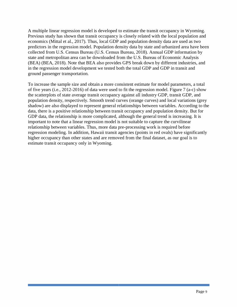
A multiple linear regression model is developed to estimate the transit occupancy in Wyoming.

Previous study has shown that transit occupancy is closely related with the local population and

economics (Mittal et al., 2017). Thus, local GDP and population density data are used as two

predictors in the regression model. Population density data by state and urbanized area have been

collected from U.S. Census Bureau (U.S. Census Bureau, 2018). Annual GDP information by

state and metropolitan area can be downloaded from the U.S. Bureau of Economic Analysis

(BEA) (BEA, 2018). Note that BEA also provides GPS break down by different industries, and

in the regression model development we tested both the total GDP and GDP in transit and

ground passenger transportation.

To increase the sample size and obtain a more consistent estimate for model parameters, a total

of five years (i.e., 2012-2016) of data were used to fit the regression model. Figure 7 (a-c) show

the scatterplots of state average transit occupancy against all industry GDP, transit GDP, and

population density, respectively. Smooth trend curves (orange curves) and local variations (grey

shadow) are also displayed to represent general relationships between variables. According to the

data, there is a positive relationship between transit occupancy and population density. But for

GDP data, the relationship is more complicated, although the general trend is increasing. It is

important to note that a linear regression model is not suitable to capture the curvilinear

relationship between variables. Thus, more data pre-processing work is required before

regression modeling. In addition, Hawaii transit agencies (points in red ovals) have significantly

higher occupancy than other states and are removed from the final dataset, as our goal is to

estimate transit occupancy only in Wyoming.

Page 10

Figure 7. Explanatory analysis for regression modeling.

Figure 7 (d-f) show the distribution of candidate predictors (i.e., all industry GDP, transit GDP,

population density). All candidate predictors have right-skewed distributions, indicating that

logarithmic transformation may be needed to normalize the data. Figure 7 (g-i) show the

scatterplots of average transit occupancy with log-transformed candidate predictors. The trend

curves for all industry GDP and transit GDP become more linear after log-transformation, while

the trend curve for population density is not significantly improved in terms of linearity. In this

report, we use log to denote the natural logarithmic transformation.

A total of five regression models were trained using different variable settings. Table 3 presents

the regression results for all five models. Model 1 takes all candidate predictors into regression,

and the result shows that all industry GDP is not significant with transit GDP already in the

model. After removing all industry GDP (Model 2), transit GDP becomes more significant as

indicated by the higher t-value. The overall model fitting is almost the same (i.e., 𝑅2 values are

very close). As mentioned in the explanatory analysis, Model 3 tested regression results with log-

transformed predictors. According to the smaller residual standard error (𝜎) and higher 𝑅2,

models with log-transformed predictors performed better than non-transformed data. Note that

log(gdp_all) shows a negative impact on transit occupancy, while in the scatterplot the trend

should be positive (as shown in Figure 7 (g)). This suggests that all industry GDP is highly

correlated with Transit GDP and should be removed to avoid multicollinearity. Models 4 and 5

tested the performance of including transit GDP and population density with different data

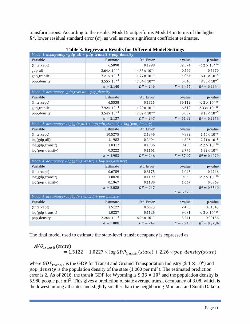
Page 11

transformations. According to the results, Model 5 outperforms Model 4 in terms of the higher

𝑅2, lower residual standard error (𝜎), as well as more significant coefficient estimates.

Table 3. Regression Results for Different Model Settings Model 1: 𝒐𝒄𝒄𝒖𝒑𝒂𝒏𝒄𝒚~𝒈𝒅𝒑_𝒂𝒍𝒍 + 𝒈𝒅𝒑_𝒕𝒓𝒂𝒏𝒔𝒊𝒕 + 𝒑𝒐𝒑_𝒅𝒆𝒏𝒔𝒊𝒕𝒚

Variable Estimate Std. Error t-value p-value

(Intercept) 6.5090 0.1998 32.574 < 2 × 10−16

gdp_all 2.64× 10−7 4.85× 10−7 0.544 0.5870

gdp_transit 7.21× 10−4 1.77× 10−4 4.064 6.48× 10−5

pop_density 3.55× 10−3 7.04× 10−4 5.045 8.80× 10−7

𝜎 = 2.140 𝐷𝐹 = 246 𝐹 = 34.55 𝑅2 = 0.2964

Model 2: 𝑜𝑐𝑐𝑢𝑝𝑎𝑛𝑐𝑦~𝑔𝑑𝑝_𝑡𝑟𝑎𝑛𝑠𝑖𝑡 + 𝑝𝑜𝑝_𝑑𝑒𝑛𝑠𝑖𝑡𝑦

Variable Estimate Std. Error t-value p-value

(Intercept) 6.5538 0.1815 36.112 < 2 × 10−16

gdp_transit 7.92× 10−4 1.20× 10−4 6.612 2.33× 10−10

pop_density 3.54× 10−3 7.02× 10−4 5.037 9.13× 10−7

𝜎 = 2.137 𝐷𝐹 = 247 𝐹 = 51.82 𝑅2 = 0.2956

Model 3: 𝑜𝑐𝑐𝑢𝑝𝑎𝑛𝑐𝑦~𝑙𝑜𝑔(𝑔𝑑𝑝_𝑎𝑙𝑙) + 𝑙𝑜𝑔(𝑔𝑑𝑝_𝑡𝑟𝑎𝑛𝑠𝑖𝑡) + 𝑙𝑜𝑔(𝑝𝑜𝑝_𝑑𝑒𝑛𝑠𝑖𝑡𝑦)

Variable Estimate Std. Error t-value p-value

(Intercept) 10.5275 2.1346 4.932 1.50× 10−6

log(gdp_all) -1.1982 0.2494 -4.803 2.71× 10−6

log(gdp_transit) 1.8317 0.1936 9.459 < 2 × 10−16

log(pop_density) 0.3222 0.1161 2.776 5.92× 10−3

𝜎 = 1.953 𝐷𝐹 = 246 𝐹 = 57.97 𝑅2 = 0.4070

Model 4: 𝑜𝑐𝑐𝑢𝑝𝑎𝑛𝑐𝑦~𝑙𝑜𝑔(𝑔𝑑𝑝_𝑡𝑟𝑎𝑛𝑠𝑖𝑡) + 𝑙𝑜𝑔(𝑝𝑜𝑝_𝑑𝑒𝑛𝑠𝑖𝑡𝑦)

Variable Estimate Std. Error t-value p-value

(Intercept) 0.6759 0.6175 1.095 0.2748

log(gdp_transit) 1.0828 0.1199 9.033 < 2 × 10−16

log(pop_density) 0.1967 0.1180 1.667 0.0969

𝜎 = 2.038 𝐷𝐹 = 247 𝐹 = 69.23

𝑅2 = 0.3540

Model 5: 𝑜𝑐𝑐𝑢𝑝𝑎𝑛𝑐𝑦~𝑙𝑜𝑔(𝑔𝑑𝑝_𝑡𝑟𝑎𝑛𝑠𝑖𝑡) + 𝑝𝑜𝑝_𝑑𝑒𝑛𝑠𝑖𝑡𝑦

Variable Estimate Std. Error t-value p-value

(Intercept) 1.5122 0.6073 2.490 0.01343

log(gdp_transit) 1.0227 0.1126 9.081 < 2 × 10−16

pop_density 2.26× 10−3 6.96× 10−4 3.241 0.00136

𝜎 = 2.008 𝐷𝐹 = 247 𝐹 = 75.19 𝑅2 = 0.3784

The final model used to estimate the state-level transit occupancy is expressed as

𝐴𝑉𝑂𝑡𝑟𝑎𝑛𝑠𝑖𝑡(𝑠𝑡𝑎𝑡𝑒)= 1.5122 + 1.0227 × log 𝐺𝐷𝑃𝑡𝑟𝑎𝑛𝑠𝑖𝑡(𝑠𝑡𝑎𝑡𝑒) + 2.26 × 𝑝𝑜𝑝_𝑑𝑒𝑛𝑠𝑖𝑡𝑦(𝑠𝑡𝑎𝑡𝑒)

where 𝐺𝐷𝑃𝑡𝑟𝑎𝑛𝑠𝑖𝑡 is the GDP for Transit and Ground Transportation Industry ($ 1 × 106) and

𝑝𝑜𝑝_𝑑𝑒𝑛𝑠𝑖𝑡𝑦 is the population density of the state (1,000 per mi2). The estimated prediction

error is 2. As of 2016, the transit GDP for Wyoming is $ 33 × 106 and the population density is

5.980 people per mi2. This gives a prediction of state average transit occupancy of 3.08, which is

the lowest among all states and slightly smaller than the neighboring Montana and South Dakota.

Page 12

Above illustrates the general procedure for estimate state-level transit bus occupancy when the

data is missing. However, given that there is no urbanized area in Wyoming, it’s might be more

appropriate to fit the regression model only using nearby states that are more similar to

Wyoming in terms of transit GDP and population density. Thus, for estimating Wyoming transit

bus occupancy, we just focused on the nearby seven states (i.e., Idaho, Montana, North Dakota,

South Dakota, Nebraska, Colorado, and Utah) that are relatively less-populated. Although

Colorado, and Utah have some large urbanized areas, these two states are included to ensure

sufficient variations in model input. The final model used to specifically estimate the transit bus

occupancy in Wyoming is expressed as

𝐴𝑉𝑂𝑡𝑟𝑎𝑛𝑠𝑖𝑡(𝑠𝑡𝑎𝑡𝑒)= 0.3353 + 0.9294 × log 𝐺𝐷𝑃𝑡𝑟𝑎𝑛𝑠𝑖𝑡(𝑠𝑡𝑎𝑡𝑒) + 55.24 × 𝑝𝑜𝑝_𝑑𝑒𝑛𝑠𝑖𝑡𝑦(𝑠𝑡𝑎𝑡𝑒)

Plug in the 2016 transit GDP and population density in Wyoming, the estimated Wyoming

average transit bus occupancy is 3.92 (as shown in Figure 8), which is slightly higher than the

regression estimate using all states as model input.

Figure 8. Average transit bus occupancy by state with Wyoming.

Urbanized area level

For data at the urbanized area level, transit agencies can be mapped into the corresponding

urbanized area based on the zip code information. The NTD transit agencies have covered 161 of

Page 13

the total 183 urbanized areas considered in this project. For urbanized areas not covered by NTD

data, a linear regression model was developed to estimate the average transit bus occupancy.

Although U.S. BEA also has GDP summarized at the metropolitan statistical area (MSA) level,

the data cannot be further broken down to the urbanized area level. Additionally, the MSA-level

transit GDP data are missing in some areas, especially in small MSAs where the NTD

information is also missing. Thus, we used the population density as the only predictor in the

regression model to estimate the urban area level transit bus occupancy. Using calculated

average transit bus occupancy for urbanized areas with NTD agencies, the fitted regression

model is expressed as below

𝐴𝑉𝑂𝑡𝑟𝑎𝑛𝑠𝑖𝑡(𝑢𝑟𝑏𝑎𝑛_𝑎𝑟𝑒𝑎) = −19.2956 + 3.3793 × log 𝑝𝑜𝑝_𝑑𝑒𝑛𝑠𝑖𝑡𝑦(𝑢𝑟𝑏𝑎𝑛_𝑎𝑟𝑒𝑎)

For the 22 urbanized areas where NTD information is missing, the average transit bus occupancy

was estimated using the above equation. The average transit bus annual mileage was assumed to

be the same as that in the corresponding state.

Table 4 summarizes the average transit occupancy results for top 20 urbanized areas (in terms of

population).

Table 4. Transit Occupancy Results for Top 20 Urbanized Areas Area Name State Average Occupancy Average VMT (mi)

New York--Newark, NY--NJ--CT New York 12.99 24109

Los Angeles--Long Beach--Anaheim, CA California 15.81 29005

Chicago, IL--IN Illinois 8.64 28313

New York--Newark, NY--NJ--CT New Jersey 15.61 31311

Miami, FL Florida 8.62 35389

Dallas--Fort Worth--Arlington, TX Texas 5.57 36521

Houston, TX Texas 4.84 16412

Atlanta, GA Georgia 9.65 30390

Boston, MA--NH--RI Massachusetts 8.29 23315

Philadelphia, PA--NJ--DE--MD Pennsylvania 12.74 27210

Detroit, MI Michigan 10.17 33035

Phoenix--Mesa, AZ Arizona 7.02 32654

San Francisco--Oakland, CA California 11.74 24422

Seattle, WA Washington 14.27 26910

San Diego, CA California 8.82 30955

Minneapolis--St. Paul, MN--WI Minnesota 7.29 29334

Tampa--St. Petersburg, FL Florida 7.43 33762

Denver--Aurora, CO Colorado 8.31 32630

Washington, DC--VA--MD Virginia 8.98 26418

Baltimore, MD Maryland 11.01 29012

Methodology: School Bus

Data Sources

The U.S. State by State Transportation Statistics 2015-16 reported by SchoolBusFleet.com (Data

Source: http://files.schoolbusfleet.com/stats/SBFFB18StateByState.pdf) is employed to calculate

the school bus occupancy for state level. The report provides a breakdown of information for

Page 14

each of the 50 states, including the number of K-12 public and private school students

transported daily, the number of school buses in each state and the total state aid paid for pupil

transportation. The data is updated annually, so it is straight forward to use the new data with our

developed methodology. Figure 9 shows an example of the data table in the report. In our

method, the public K-12 students transported daily and the total annual route mileage are

employed as the input data. Based on the data reported from American School Bus Council

(ASBC) (Data Source: http://www.americanschoolbuscouncil.org/issues/environmental-

benefits), we can know the following two important information: (1) Average distance from home to school for bus riders (ASBC estimate, miles) = 5 miles

(2) Length of average school year (days) = 180 days

Figure 9. Sample data of the U.S. State by State Transportation Statistics 2015-16. Source:

http://files.schoolbusfleet.com/stats/SBFFB18StateByState.pdf.

Method for Estimating Occupancy Factors

State level

As a result, the average school bus occupancy for each state can be estimated based on the

following equation:

𝐴𝑉𝑂𝑠𝑐ℎ𝑜𝑜𝑙 =∑ 𝑃𝑀𝑇𝑖𝑖

∑ 𝑉𝑀𝑇𝑖𝑖+ 1 =

𝑁𝑢𝑚𝑏𝑒𝑟 𝑜𝑓 𝑆𝑡𝑢𝑑𝑒𝑛𝑡 𝑇𝑟𝑎𝑛𝑠𝑝𝑜𝑟𝑡𝑒𝑑 𝐷𝑎𝑖𝑙𝑦 × 180 × (5 × 2)

𝑇𝑜𝑡𝑎𝑙 𝐴𝑛𝑛𝑢𝑎𝑙 𝑅𝑜𝑢𝑡𝑒 𝑀𝑖𝑙𝑒𝑎𝑔𝑒+ 1

where (5 × 2) is the average round trip distance from home to school. The estimated average

school bus occupancy for the states are summarized in Figure 10. The total annual route mileage

data are missing for 14 states, and these states require additional model to estimate the average

school bus occupancy.

Page 15

Figure 10. Average school bus occupancy by state (14 states missing).

To address the missing data issue, a local factors-based weighted model is developed by

incorporating local factors such as total school enrollment, average district enrollment, total

districts, total schools, total students transported daily, total yellow school buses as below

𝐴𝑉𝑂𝑠𝑐ℎ𝑜𝑜𝑙(𝑆𝑡𝑎𝑡𝑒 𝑖) = ∑ 𝑤(𝑖, 𝑗) × 𝐴𝑉𝑂𝑠𝑐ℎ𝑜𝑜𝑙(𝑆𝑡𝑎𝑡𝑒 𝑗)

𝑁

𝑗=1

where the weight 𝑤(𝑖, 𝑗) is defined as an index to describe the similarity between state i and state

j. If the local factors of state i is close to those of state j, the similarity between them is high

which implies a high value of weight 𝑤(𝑖, 𝑗). Let 𝐹𝑙(i) be a local factor of state i, then the weight

𝑤(𝑖, 𝑗) can be defined as

𝑤(𝑖, 𝑗) =∑ (1 −

|𝐹𝑙(i) − 𝐹𝑙(j)|𝑚𝑎𝑥{𝐹𝑙(i), 𝐹𝑙(j)}

)𝐿𝑙=1

∑ ∑ (1 −|𝐹𝑙(i) − 𝐹𝑙(j)|

𝑚𝑎𝑥{𝐹𝑙(i), 𝐹𝑙(j)})𝐿

𝑙=1𝑁𝑗=1

where the design of the item |𝐹𝑙(i)−𝐹𝑙(j)|

𝑚𝑎𝑥{𝐹𝑙(i),𝐹𝑙(j)} can guarantee that the value ranges between 0 and 1.

The data for these local factors can be found from SchoolBusFleet.com (Data Source:

http://files.schoolbusfleet.com/stats/SBFFB18StateByState.pdf) and Governing.com (Data

Source: http://www.governing.com/gov-data/education-data/school-district-totals-average-

enrollment-statistics-for-states-metro-areas.html). By using weight 𝑤(𝑖, 𝑗), the state has similar

local factors will have more impacts on the estimation of the average school bus occupancy for

Page 16

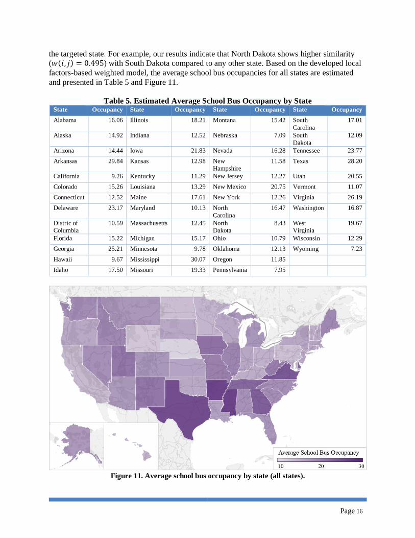
the targeted state. For example, our results indicate that North Dakota shows higher similarity

(𝑤(𝑖, 𝑗) = 0.495) with South Dakota compared to any other state. Based on the developed local

factors-based weighted model, the average school bus occupancies for all states are estimated

and presented in Table 5 and Figure 11.

Table 5. Estimated Average School Bus Occupancy by State State Occupancy State Occupancy State Occupancy State Occupancy

Alabama 16.06 Illinois 18.21 Montana 15.42 South

Carolina

17.01

Alaska 14.92 Indiana 12.52 Nebraska 7.09 South

Dakota

12.09

Arizona 14.44 Iowa 21.83 Nevada 16.28 Tennessee 23.77

Arkansas 29.84 Kansas 12.98 New Hampshire

11.58 Texas 28.20

California 9.26 Kentucky 11.29 New Jersey 12.27 Utah 20.55

Colorado 15.26 Louisiana 13.29 New Mexico 20.75 Vermont 11.07

Connecticut 12.52 Maine 17.61 New York 12.26 Virginia 26.19

Delaware 23.17 Maryland 10.13 North

Carolina

16.47 Washington 16.87

Distric of Columbia

10.59 Massachusetts 12.45 North Dakota

8.43 West Virginia

19.67

Florida 15.22 Michigan 15.17 Ohio 10.79 Wisconsin 12.29

Georgia 25.21 Minnesota 9.78 Oklahoma 12.13 Wyoming 7.23

Hawaii 9.67 Mississippi 30.07 Oregon 11.85

Idaho 17.50 Missouri 19.33 Pennsylvania 7.95

Figure 11. Average school bus occupancy by state (all states).

Page 17

Urbanized area level

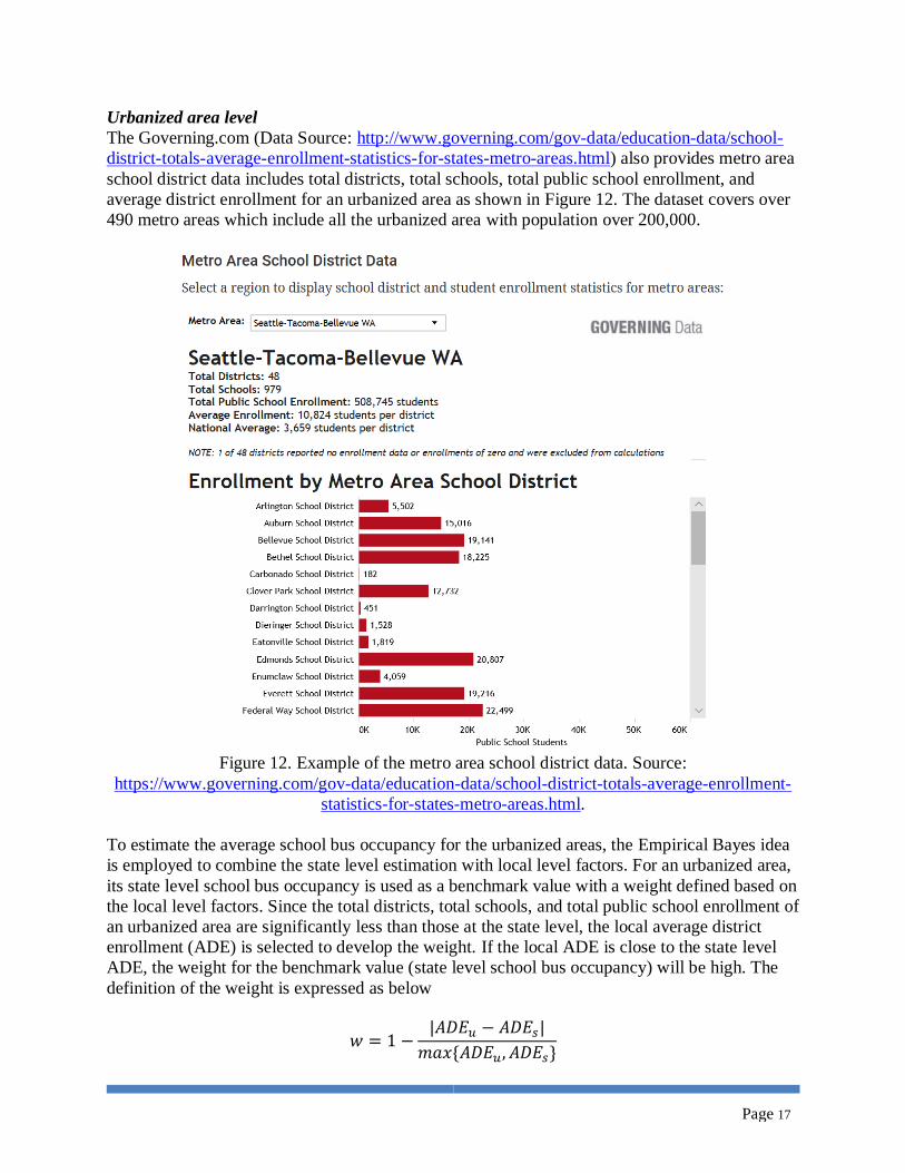
The Governing.com (Data Source: http://www.governing.com/gov-data/education-data/school-

district-totals-average-enrollment-statistics-for-states-metro-areas.html) also provides metro area

school district data includes total districts, total schools, total public school enrollment, and

average district enrollment for an urbanized area as shown in Figure 12. The dataset covers over

490 metro areas which include all the urbanized area with population over 200,000.

Figure 12. Example of the metro area school district data. Source:

https://www.governing.com/gov-data/education-data/school-district-totals-average-enrollment-

statistics-for-states-metro-areas.html.

To estimate the average school bus occupancy for the urbanized areas, the Empirical Bayes idea

is employed to combine the state level estimation with local level factors. For an urbanized area,

its state level school bus occupancy is used as a benchmark value with a weight defined based on

the local level factors. Since the total districts, total schools, and total public school enrollment of

an urbanized area are significantly less than those at the state level, the local average district

enrollment (ADE) is selected to develop the weight. If the local ADE is close to the state level

ADE, the weight for the benchmark value (state level school bus occupancy) will be high. The

definition of the weight is expressed as below

𝑤 = 1 −|𝐴𝐷𝐸𝑢 − 𝐴𝐷𝐸𝑠|

𝑚𝑎𝑥{𝐴𝐷𝐸𝑢, 𝐴𝐷𝐸𝑠}

Page 18

where 𝐴𝐷𝐸𝑢 is the average district enrollment for an urbanized area, 𝐴𝐷𝐸𝑠 is the average district

enrollment for the corresponding state. Therefore, the empirical Bayes model for estimating the

urbanized area average school bus occupancy is developed as below

𝐴𝑉𝑂𝑠𝑐ℎ𝑜𝑜𝑙(𝑢𝑟𝑏𝑎𝑛_𝑎𝑟𝑒𝑎) = 𝑤 × 𝐴𝑉𝑂𝑠𝑐ℎ𝑜𝑜𝑙(𝑠𝑡𝑎𝑡𝑒) + (1 − 𝑤) × 𝐸𝐴𝑉𝑂𝑠𝑐ℎ𝑜𝑜𝑙(𝑢𝑟𝑏𝑎𝑛_𝑎𝑟𝑒𝑎)

where 𝐸𝐴𝑉𝑂𝑆𝑐ℎ𝑜𝑜𝑙(𝑢𝑟𝑏𝑎𝑛_𝑎𝑟𝑒𝑎) is the expected average school bus occupancy for the

urbanized area. In order to estimate 𝐸𝐴𝑉𝑂𝑆𝑐ℎ𝑜𝑜𝑙(𝑢𝑟𝑏𝑎𝑛_𝑎𝑟𝑒𝑎), the factors such as total districts,

total schools, total public school enrollment, and average district enrollment are explored to

identify their relationship with the average school bus occupancy as shown in Figure 13. The

state level data including total districts, total schools, total public school enrollment, and average

district enrollment are used to establish the regression models to estimate the average school bus

occupancy. The outliers such as California, Texas, Nevada, Florida, Maryland (points in red

ovals) that have significant higher values than other states are removed from the final datasets.

Five different regression models including linear regression, log regression exponential

regression, polynomial regression, and power regression are tested based on the final datasets for

different factors. The models with best performance are selected and shown in Figure 13.

Page 19

Figure 13. Regression analysis for urbanized area level school bus occupancy estimation.

The results show that the log regression model based on the final dataset of average district

enrollment performances best as compared to the other models (𝑅2 = 0.1309). As a result, the

0

5

10

15

20

25

30

35

0 10,000 20,000 30,000 40,000 50,000

y = 2.5376ln(x) - 1.851R² = 0.1309

0

5

10

15

20

25

30

35

0 2,000 4,000 6,000 8,000 10,000 12,000 14,000 16,000

Ave

rage

Sch

oo

l Bu

s O

ccu

pan

cy

Average District Enrollment Average District Enrollment

0

5

10

15

20

25

30

35

0 1,000,000 2,000,000 3,000,000 4,000,000 5,000,000 6,000,000 7,000,000

Ave

rage

Sch

oo

l Bu

s O

ccu

pan

cy

Texas

California

Florida

MarylandNevada

Florida

0

5

10

15

20

25

30

35

0 200 400 600 800 1000 1200

Total Enrolled Students

Total Districts

Ave

rage

Sch

oo

l Bu

s O

ccu

pan

cy

Texas

California

0

5

10

15

20

25

30

35

0 2,000 4,000 6,000 8,000 10,000 12,000

Ave

rage

Sch

oo

l Bu

s O

ccu

pan

cy

Total Schools

California

Texas

y = -0.007x + 20.014R² = 0.0348

0

5

10

15

20

25

30

35

0 100 200 300 400 500 600

Total Districts

y = -9E-07x2 + 0.0034x + 16.44R² = 0.036

0

5

10

15

20

25

30

35

0 500 1,000 1,500 2,000 2,500 3,000 3,500 4,000 4,500

Total Schools

y = 3.7316x0.1191

R² = 0.0938

0

5

10

15

20

25

30

35

0 500,000 1,000,000 1,500,000 2,000,000

Total Enrolled Students

Page 20

final model used to estimate the expected average school bus occupancy for the urbanized areas

is expressed as

𝐸𝐴𝑉𝑂𝑠𝑐ℎ𝑜𝑜𝑙(𝑢𝑟𝑏𝑎𝑛_𝑎𝑟𝑒𝑎) = 2.5376 × log 𝐴𝐷𝐸𝑢 − 1.851

Based on the above method, the average school bus occupancy for all the urbanized areas

required in the project can be estimated. The average school bus occupancy rates for top 20

urbanized areas are presented in Table 6.

Table 6. School Bus Occupancy Results for Top 20 Urbanized Areas

Area Name State Average Occupancy Average VMT (mi)

New York--Newark, NY--NJ--CT New York 13.82 12000

Los Angeles--Long Beach--Anaheim, CA California 17.32 10509

Chicago, IL--IN Illinois 18.78 7553

New York--Newark, NY--NJ--CT New Jersey 13.78 12000

Miami, FL Florida 22.26 17219

Dallas--Fort Worth--Arlington, TX Texas 24.57 2477

Houston, TX Texas 24.45 2477

Atlanta, GA Georgia 24.38 9642

Boston, MA--NH--RI Massachusetts 13.01 12000

Philadelphia, PA--NJ--DE--MD Pennsylvania 7.99 18253

Detroit, MI Michigan 17.78 10212

Phoenix--Mesa, AZ Arizona 15.33 11253

San Francisco--Oakland, CA California 10.10 10509

Seattle, WA Washington 19.94 12529

San Diego, CA California 14.94 10509

Minneapolis--St. Paul, MN--WI Minnesota 15.94 13919

Tampa--St. Petersburg, FL Florida 21.68 17219

Denver--Aurora, CO Colorado 19.92 12356

Washington, DC--VA--MD Virginia 25.42 7680

Baltimore, MD Maryland 12.44 17262

As an alternative method to estimate the school bus occupancy, we also conducted surveys to get

local data for school bus occupancy related information. Such information includes the minimum

busing distance, total travel distance, and school bus loading factor. Survey results were

collected from two urbanized areas, Milwaukee and Madison in Wisconsin, and summarized in

Table 7. The distribution of school bus capacity is mined from Polk data and based on the

vehicle model and manufacturer website (as shown in Figure 14). The average school bus

capacity for Milwaukee and Madison are 72.29 and 76.82, respectively.

Table 7. School Bus Occupancy Survey Results from Milwaukee and Madison Variable Item Milwaukee Madison

𝑑𝑚𝑖𝑛 Minimum busing distance 0.5 mile 1 mile

𝑑𝑡𝑜𝑡𝑎𝑙 Total travel distance 12 mile 15 mile

𝐿 School bus loading factor 85 % 80 %

𝐶 Average school bus capacity 72.29 76.82

Page 21

Figure 14. Example of school bus capacity information from the website. Source:

https://www.blue-bird.com/buses.

To calculate the average school bus occupancy, Figure 15 shows the change of school bus

loading rate during a typical route. During the morning peak trip, the school bus is assumed to

leave the base station and go to pick up students one by one. The loading ratio will gradually

increase until arrives the peak level (usually around 75%-95%). After the school bus picked up

the last student, it will travel another minimum bussing distance and eventually let all the student

get off at the school. Then it will go back to the base station with empty load. Therefore, the

average loading factor during the route should be

Figure 15. Changes of school bus loading ratio during a typical route (morning peak).

�̅� =

𝐿2

2𝑟+ 𝐿 × 𝑑𝑚𝑖𝑛

𝑑𝑡𝑜𝑡𝑎𝑙

Page 22

Further assume that the school bus base is located or very close to the school served, then the

length of the outbound trip with only the driver would be approximately equal to the length of

the trip back to school with students. This is expressed as

𝐿

𝑟+ 𝑑𝑚𝑖𝑛 =

𝑑𝑡𝑜𝑡𝑎𝑙

2

This gives the average loading factor as

�̅� = (1

4+

𝑑𝑚𝑖𝑛

2𝑑𝑡𝑜𝑡𝑎𝑙) 𝐿

So the school bus occupancy can be calculated as

𝐴𝑉𝑂𝑆𝑐ℎ𝑜𝑜𝑙 = 1 + 𝐶 × �̅�

Based on the above model, the estimated average school bus occupancy for Milwaukee and

Madison are 17.65 and 18.39, respectively.

Methodology: Motorcoach (Private Bus)

Data Sources

The Port Authority of New York and New Jersey (PANYNJ) provided motorcoach and

passenger hourly arrivals and departures data at the Port Authority Bus Terminal (PABT) for

2015. The PABT data were collected by surveying bus carriers who have direct service to

PANYNJ, and the annual survey results can be requested periodically. This dataset covers 24

states and 35 urbanized areas. The PABT is the main gateway for interstate buses into Manhattan

in New York City. The PABT is located in Midtown at 625 Eighth Avenue between 40th Street

and 42nd Street, one block east of the Lincoln Tunnel and one block west of Times Square. It is

one of three bus terminals operated by the PANYNJ, the others being the George Washington

Bridge Bus Station in Upper Manhattan and the Journal Square Transportation Center in Jersey

City. The PABT serves as a terminus and departure point for commuter routes as well as for

long-distance intercity routes and is a major transit hub.

The Motorcoach Census Report 2015 developed by American Bus Association Foundation and

John Dunham & Associates are also used as a data source to obtain the national level motorcoach

occupancy information (American Bus Association. 2017). Additionally, some local reports such

as Motor Coach Tourism in Savannah produced by the Armstrong Atlantic State University for

the City of Savannah are also referenced as alternative methods to estimate the urbanized area

level motorcoach occupancy (Armstrong Atlantic State University. 2013).

Method for Estimating Occupancy Factors

State level

The Port Authority Bus Terminal data included detailed total bus and passenger hourly arrivals

and departures for 256 routes identified by origin and destination. The motorcoach occupancy for

a route can be estimated by using the following equation

Page 23

𝐴𝑉𝑂𝑚𝑜𝑡𝑜𝑟𝑐𝑜𝑎𝑐ℎ(𝑟𝑜𝑢𝑡𝑒) =𝐷𝑎𝑖𝑙𝑦 𝑃𝑎𝑠𝑠𝑒𝑛𝑔𝑒𝑟 𝐷𝑒𝑝𝑎𝑟𝑡𝑢𝑟𝑒𝑠 + 𝐷𝑎𝑖𝑙𝑦 𝑃𝑎𝑠𝑠𝑒𝑛𝑔𝑒𝑟 𝐴𝑟𝑟𝑖𝑣𝑎𝑙𝑠

𝐷𝑎𝑖𝑙𝑦 𝐵𝑢𝑠 𝐷𝑒𝑝𝑎𝑟𝑡𝑢𝑟𝑒𝑠 + 𝐷𝑎𝑖𝑙𝑦 𝐵𝑢𝑠 𝐴𝑟𝑟𝑖𝑣𝑎𝑙𝑠+ 1

Here both the arrivals and departures data are used to estimate the average motorcoach occupancy. Since

the interstate bus usually goes across several states, the average motorcoach occupancy for a state can be

estimated by using the following equation

𝐴𝑉𝑂𝑚𝑜𝑡𝑜𝑟𝑐𝑜𝑎𝑐ℎ(𝑠𝑡𝑎𝑡𝑒) =∑ 𝐴𝑉𝑂𝑚𝑜𝑡𝑜𝑟𝑐𝑜𝑎𝑐ℎ(𝑟𝑜𝑢𝑡𝑒) × 𝑏𝑢𝑠_𝑐𝑜𝑢𝑛𝑡(𝑟𝑜𝑢𝑡𝑒)𝑟𝑜𝑢𝑡𝑒 ∋ 𝑠𝑡𝑎𝑡𝑒

∑ 𝑏𝑢𝑠_𝑐𝑜𝑢𝑛𝑡(𝑟𝑜𝑢𝑡𝑒)𝑟𝑜𝑢𝑡𝑒 ∋ 𝑠𝑡𝑎𝑡𝑒

where 𝑟𝑜𝑢𝑡𝑒 ∋ 𝑠𝑡𝑎𝑡𝑒 represents aggregating across all routes that pass the state. Based on the

above model, the average motorcoach occupancies for 25 states are estimated as shown in Table

8 and Figure 16.

Table 8. Estimated Average Motorcoach Occupancy by State

State Occupancy State Occupancy State Occupancy State Occupancy

Alabama 47.48 Illinois 47.13 Montana NA Rhode Island

44.03

Alaska NA Indiana NA Nebraska NA South

Carolina

45.23

Arizona NA Iowa NA Nevada NA South

Dakota

NA

Arkansas NA Kansas NA New Hampshire

41.09 Tennessee 47.48

California 33.40 Kentucky 45.81 New Jersey 29.47 Texas NA

Colorado NA Louisiana NA New Mexico NA Utah NA

Connecticut 38.94 Maine 38.00 New York 31.86 Vermont NA

Delaware 39.28 Maryland 48.19 North

Carolina

45.03 Virginia 42.71

District of

Columbia

48.32 Massachusetts 44.19 North

Dakota

NA Washington NA

Florida 40.31 Michigan 40.69 Ohio 43.42 West

Virginia

NA

Georgia 41.53 Minnesota NA Oklahoma NA Wisconsin NA

Hawaii NA Mississippi NA Oregon NA Wyoming NA

Idaho NA Missouri 33.40 Pennsylvania 38.19

Page 24

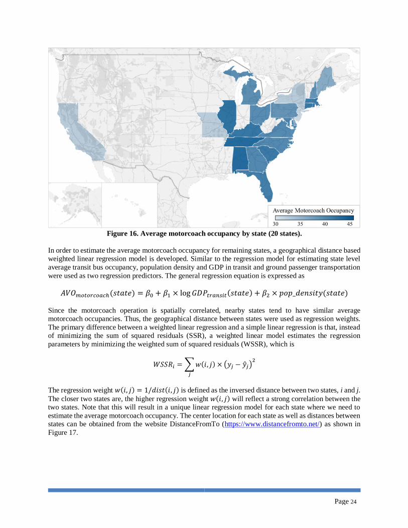
Figure 16. Average motorcoach occupancy by state (20 states).

In order to estimate the average motorcoach occupancy for remaining states, a geographical distance based

weighted linear regression model is developed. Similar to the regression model for estimating state level

average transit bus occupancy, population density and GDP in transit and ground passenger transportation

were used as two regression predictors. The general regression equation is expressed as

𝐴𝑉𝑂𝑚𝑜𝑡𝑜𝑟𝑐𝑜𝑎𝑐ℎ(𝑠𝑡𝑎𝑡𝑒) = 𝛽0 + 𝛽1 × log 𝐺𝐷𝑃𝑡𝑟𝑎𝑛𝑠𝑖𝑡(𝑠𝑡𝑎𝑡𝑒) + 𝛽2 × 𝑝𝑜𝑝_𝑑𝑒𝑛𝑠𝑖𝑡𝑦(𝑠𝑡𝑎𝑡𝑒)

Since the motorcoach operation is spatially correlated, nearby states tend to have similar average

motorcoach occupancies. Thus, the geographical distance between states were used as regression weights.

The primary difference between a weighted linear regression and a simple linear regression is that, instead

of minimizing the sum of squared residuals (SSR), a weighted linear model estimates the regression

parameters by minimizing the weighted sum of squared residuals (WSSR), which is

𝑊𝑆𝑆𝑅𝑖 = ∑ 𝑤(𝑖, 𝑗) × (𝑦𝑗 − �̂�𝑗)2

𝑗

The regression weight 𝑤(𝑖, 𝑗) = 1/𝑑𝑖𝑠𝑡(𝑖, 𝑗) is defined as the inversed distance between two states, i and j.

The closer two states are, the higher regression weight 𝑤(𝑖, 𝑗) will reflect a strong correlation between the

two states. Note that this will result in a unique linear regression model for each state where we need to

estimate the average motorcoach occupancy. The center location for each state as well as distances between

states can be obtained from the website DistanceFromTo (https://www.distancefromto.net/) as shown in

Figure 17.

Page 25

Figure 17. Example of calculating distance between two states using DistanceFromTo. Source:

https://www.distancefromto.net/.

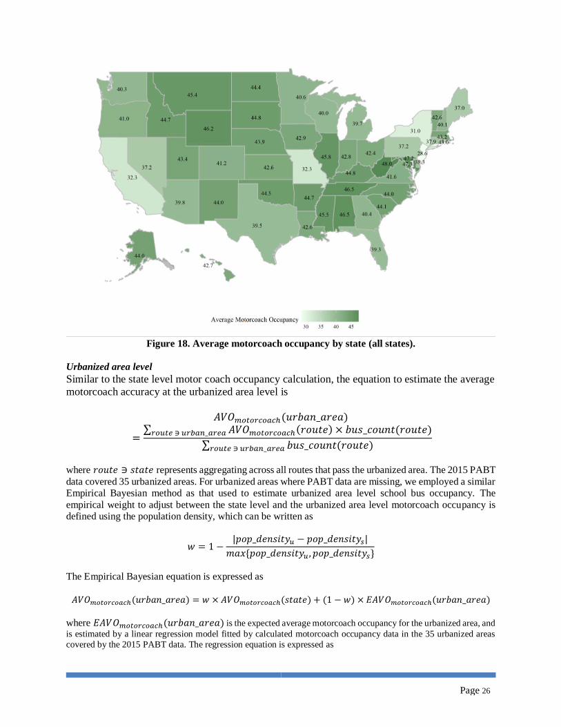
The complete state level average motorcoach occupancy is presented in Figure 18. In general, the average

motorcoach occupancy is higher in less populated areas and lower in more populated areas. According to

the 2015 Motorcoach Census Report, the national average motorcoach occupancy is 36.4, which generally

agrees with the results estimated using PABT data.

Page 26

Figure 18. Average motorcoach occupancy by state (all states).

Urbanized area level

Similar to the state level motor coach occupancy calculation, the equation to estimate the average

motorcoach accuracy at the urbanized area level is

𝐴𝑉𝑂𝑚𝑜𝑡𝑜𝑟𝑐𝑜𝑎𝑐ℎ(𝑢𝑟𝑏𝑎𝑛_𝑎𝑟𝑒𝑎)

=∑ 𝐴𝑉𝑂𝑚𝑜𝑡𝑜𝑟𝑐𝑜𝑎𝑐ℎ(𝑟𝑜𝑢𝑡𝑒) × 𝑏𝑢𝑠_𝑐𝑜𝑢𝑛𝑡(𝑟𝑜𝑢𝑡𝑒)𝑟𝑜𝑢𝑡𝑒 ∋ 𝑢𝑟𝑏𝑎𝑛_𝑎𝑟𝑒𝑎

∑ 𝑏𝑢𝑠_𝑐𝑜𝑢𝑛𝑡(𝑟𝑜𝑢𝑡𝑒)𝑟𝑜𝑢𝑡𝑒 ∋ 𝑢𝑟𝑏𝑎𝑛_𝑎𝑟𝑒𝑎

where 𝑟𝑜𝑢𝑡𝑒 ∋ 𝑠𝑡𝑎𝑡𝑒 represents aggregating across all routes that pass the urbanized area. The 2015 PABT

data covered 35 urbanized areas. For urbanized areas where PABT data are missing, we employed a similar

Empirical Bayesian method as that used to estimate urbanized area level school bus occupancy. The

empirical weight to adjust between the state level and the urbanized area level motorcoach occupancy is

defined using the population density, which can be written as

𝑤 = 1 −|𝑝𝑜𝑝_𝑑𝑒𝑛𝑠𝑖𝑡𝑦𝑢 − 𝑝𝑜𝑝_𝑑𝑒𝑛𝑠𝑖𝑡𝑦𝑠|

𝑚𝑎𝑥{𝑝𝑜𝑝_𝑑𝑒𝑛𝑠𝑖𝑡𝑦𝑢 , 𝑝𝑜𝑝_𝑑𝑒𝑛𝑠𝑖𝑡𝑦𝑠}

The Empirical Bayesian equation is expressed as

𝐴𝑉𝑂𝑚𝑜𝑡𝑜𝑟𝑐𝑜𝑎𝑐ℎ(𝑢𝑟𝑏𝑎𝑛_𝑎𝑟𝑒𝑎) = 𝑤 × 𝐴𝑉𝑂𝑚𝑜𝑡𝑜𝑟𝑐𝑜𝑎𝑐ℎ(𝑠𝑡𝑎𝑡𝑒) + (1 − 𝑤) × 𝐸𝐴𝑉𝑂𝑚𝑜𝑡𝑜𝑟𝑐𝑜𝑎𝑐ℎ(𝑢𝑟𝑏𝑎𝑛_𝑎𝑟𝑒𝑎)

where 𝐸𝐴𝑉𝑂𝑚𝑜𝑡𝑜𝑟𝑐𝑜𝑎𝑐ℎ(𝑢𝑟𝑏𝑎𝑛_𝑎𝑟𝑒𝑎) is the expected average motorcoach occupancy for the urbanized area, and

is estimated by a linear regression model fitted by calculated motorcoach occupancy data in the 35 urbanized areas

covered by the 2015 PABT data. The regression equation is expressed as

Page 27

𝐸𝐴𝑉𝑂𝑚𝑜𝑡𝑜𝑟𝑐𝑜𝑎𝑐ℎ(𝑢𝑟𝑏𝑎𝑛_𝑎𝑟𝑒𝑎) = 45.705 − 0.761 × log 𝑝𝑜𝑝_𝑑𝑒𝑛𝑠𝑖𝑡𝑦(𝑢𝑟𝑏𝑎𝑛_𝑎𝑟𝑒𝑎)

Following the Empirical Bayesian equation, the estimated average motorcoach occupancy rates for top 20

urbanized areas are presented in Table 9.

Table 9. Motorcoach Occupancy Results for Top 20 Urbanized Areas Area Name State Average Occupancy

New York--Newark, NY--NJ--CT New York 31.86

Los Angeles--Long Beach--Anaheim, CA California 33.40

Chicago, IL--IN Illinois 47.13

New York--Newark, NY--NJ--CT New Jersey 29.37

Miami, FL Florida 36.14

Dallas--Fort Worth--Arlington, TX Texas 39.68

Houston, TX Texas 39.65

Atlanta, GA Georgia 41.35

Boston, MA--NH--RI Massachusetts 44.82

Philadelphia, PA--NJ--DE--MD Pennsylvania 45.81

Detroit, MI Michigan 40.69

Phoenix--Mesa, AZ Arizona 39.59

San Francisco--Oakland, CA California 38.84

Seattle, WA Washington 39.66

San Diego, CA California 39.03

Minneapolis--St. Paul, MN--WI Minnesota 39.77

Tampa--St. Petersburg, FL Florida 46.73

Denver--Aurora, CO Colorado 39.52

Washington, DC--VA--MD Virginia 39.75

Baltimore, MD Maryland 48.35

Some local reports such as Motor Coach Tourism in Savannah can also be used as supplementary data

sources. The report from the City of Savannah summarized motorcoach occupancy and related information

such as passengers per coach and bus type market share for different bus type in 2013 (see Figure 19). The

average motorcoach occupancy in Savannah can be directly calculated as

𝐴𝑉𝑂𝑚𝑜𝑡𝑜𝑟𝑐𝑜𝑎𝑐ℎ(𝑆𝑎𝑣𝑎𝑛𝑛𝑎ℎ) = ∑ 𝑃𝑎𝑠𝑠𝑒𝑛𝑔𝑒𝑟𝑠 𝑝𝑒𝑟 𝐶𝑜𝑎𝑐ℎ (𝑡) × 𝐵𝑢𝑠 𝑇𝑦𝑝𝑒 𝑀𝑎𝑟𝑘𝑒𝑡 𝑆ℎ𝑎𝑟𝑒 (𝑡) + 1 = 41.72

𝑇

𝑡=1

The estimated average motorcoach occupancy for Savannah in 2013 is 41.72 while the result based on the

2015 PABT data is 46.12. The estimation difference between two methods is around 10%.

Page 28

Figure 19. Occupancy related information in Motor Coach Tourism in Savannah. Source:

http://www.savannahga.gov/DocumentCenter/View/4364/FINAL-

CoachStudy_AASU_031213?bidId=.

Developing Truck Occupancy Factors

Methodology Framework

The estimation of average truck occupancy relies on accident reports. As the truck accident

dataset is usually aggregated (e.g., crashes that involve different types of truck are all included in

the same data), it’s not necessarily to calculate the average truck occupancy by each truck class.

An overall average truck occupancy number can be calculated for all truck types. According to

the project scope, pickup trucks (i.e., FHWA class 3) and 2-axle single unit trucks (FHWA class

5) are not considered in this project. Those trucks are filtered out from the crash data before

estimating the average truck occupancy. However, the methodology being introduced below is

generally applicable to all truck types, and it is straightforward to include class 3 and 5 trucks

into calculation if there is a future need.

Methodology: Truck

Data Sources

The NHTSA’s Trucks in Fatal Accidents (TIFA) data were used as the primary dataset for truck

occupancy estimation. The TIFA data were built based on cases that involved medium and heavy

trucks in Fatality Analysis Reporting System (FARS). Additional information was also provided

beyond FARS such as more accurate vehicle classification and truck details (e.g., fuel type,

weight type) processed from VIN numbers (Jarossi et al., 2012). To obtain a sufficient sample

size and improve our estimation accuracy, 5 years (i.e., 2006-2010) of TIFA data were collected

to estimate truck occupancy.

Table 10 summarized the sample size as well as the average occupancy and standard error

calculated for each year. Note that there is a general decreasing trend of truck crashes, indicating

the necessity of using data from earlier years to get enough samples. According to the table, the

average truck occupancy varies between 1.15 and 1.20 during the 5 years, and there is no

obvious change over time.

Page 29

Table 10. Summary Statistics of TIFA Data from 2006 to 2010 Year Count Average Occupancy Standard Error

2006 5250 1.209 0.573

2007 5049 1.162 0.460

2008 4352 1.179 0.514

2009 3450 1.193 0.573

2010 3699 1.174 0.508

Method for Estimating Occupancy Factors

State level

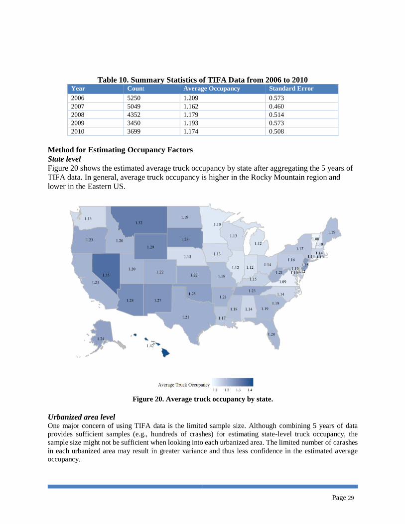
Figure 20 shows the estimated average truck occupancy by state after aggregating the 5 years of

TIFA data. In general, average truck occupancy is higher in the Rocky Mountain region and

lower in the Eastern US.

Figure 20. Average truck occupancy by state.

Urbanized area level One major concern of using TIFA data is the limited sample size. Although combining 5 years of data

provides sufficient samples (e.g., hundreds of crashes) for estimating state-level truck occupancy, the

sample size might not be sufficient when looking into each urbanized area. The limited number of carashes

in each urbanized area may result in greater variance and thus less confidence in the estimated average

occupancy.

Page 30

To overcome the data limitation issue, a Bayesian method is developed to estimate the truck occupancy

specifically for urbanized areas. The Bayesian theorem applies a rational estimate procedure that updates a

prior belief with new information. In the truck occupancy estimation task, we can regard the state-level

truck occupancy as our “prior” belief for urbanized areas within the state. Then truck crashes actually

happening in each urbanized area can be considered as the “new information” to generate more accurate

localized estimates. This method is based on the assumption that trucks observed in each urbanized area

most likely also have travelled to other areas in the same state. Additionally, local truck policies and

regulations that can possibly influence regional truck occupancy are more consistent within each state.

Thus, the state-level truck occupancy can serve as our prior belief before looking at truck crashes in each

specific urbanized area.

The equations for the Bayesian method depend on the specific distribution of the data. The overall

distribution of truck occupancy data is shown in Figure 21. Based on the distribution shape and the discrete

nature of occupancy data, Poisson distribution seems to be a good candidate to model the truck occupancy.

Note that the minimum value for truck occupancy is 1 (as we only want to consider trucks in operation),

but the minimum possible value for Poisson distribution is 0. Thus we assume the truck occupancy follows

𝑂𝑡𝑟𝑢𝑐𝑘 − 1 ~ Poisson(𝜆)

where 𝜆 = �̅�𝑡𝑟𝑢𝑐𝑘 − 1

The dashed trend line in Figure 21 shows the theoretical probability mass function (pmf) calculated from

the corresponding Poisson distribution (𝜆 = 0.184). The theoretical pmf matched pretty well with the actual

distribution of truck count, indicating that truck occupancy is approximately Poisson distributed.

Figure 21. Distribution of truck occupancy and theoretical probability.

The Bayesian equation can thus be derived based on Poisson distributed truck occupancy data.

Given 𝑂𝑡𝑟𝑢𝑐𝑘 − 1 ~ Poisson(𝜆), the joint probability of observing 𝑂𝑡1, 𝑂𝑡1, … 𝑂𝑡𝑛 is

Page 31

𝑝(𝑂𝑡1 = 𝑜𝑡1, 𝑂𝑡2 = 𝑜𝑡2, … , 𝑂𝑡𝑛 = 𝑜𝑡𝑛| 𝜆) = ∏ 𝑒−𝜆 𝜆𝑜𝑡𝑖−1

𝑜𝑡𝑖 − 1!

𝑛

𝑖=1

∝ 𝜆Σ𝑜𝑡𝑖−𝑛𝑒−𝑛𝜆

Based on Bayesian theorem

𝑝(𝜆| 𝑜𝑡1, … , 𝑜𝑡𝑛) =𝑝(𝑜𝑡1, … , 𝑜𝑡𝑛 | 𝜆) × 𝑝(𝜆)

𝑝(𝑜𝑡1, … , 𝑜𝑡𝑛)∝ 𝑝(𝜆) × 𝜆Σ𝑜𝑡𝑖−𝑛𝑒−𝑛𝜆

Thus, the density of our parameter (𝜆) estimate include terms like 𝜆c1𝑒−𝑐2𝜆. The simplest

probability distribution that includes such terms is the family of Gamma distributions, and the

corresponding probability distribution function is

𝑝(𝜆) =𝑏𝑎

Γ(𝑎)𝜆𝑎−1𝑒−𝑏𝜆

where 𝑎, 𝑏 are distribution parameters and Γ() is the Gamma function. The mean and variance of

Gamma distribution is

𝐸(𝜆) =𝑎

𝑏

𝑉𝑎𝑟(𝜆) =𝑎

𝑏2

For a particular state 𝑠𝑖, if we have observed 𝑛𝑠 truck crashes with occupancy 𝑜𝑠1, 𝑜𝑠2

, … , 𝑜𝑠𝑛𝑠,

our estimated average occupancy is Σ𝑜𝑠𝑖 𝑛𝑠⁄ , which corresponds to a parameter estimate of

𝜆𝑠 =Σ𝑜𝑠𝑖

𝑛𝑠− 1 =

Σ𝑜𝑠𝑖 − 𝑛𝑠

𝑛𝑠

Thus, the state-level parameter 𝜆𝑠 follows a Gamma distribution with 𝑎𝑠 = Σ𝑜𝑠𝑖 − 𝑛𝑠 and 𝑏𝑠 =𝑛𝑠. Use this as our prior belief of 𝜆. For an urbanized area within this state, if we have 𝑛𝑢 truck

crashes with occupancy 𝑜𝑢1, 𝑜𝑢2

, … , 𝑜𝑢𝑛𝑢, then the posterior distribution of 𝜆 is

𝑝(𝜆| 𝑜𝑢1, … , 𝑜𝑢𝑛𝑢

) ∝ 𝑝(𝜆) × 𝜆Σ𝑜𝑢𝑗−𝑛𝑢𝑒−𝑛𝑢𝜆 ∝ 𝜆𝑎𝑠−1𝑒−𝑏𝑠𝜆 × 𝜆Σ𝑜𝑢𝑗−𝑛𝑢𝑒−𝑛𝑢𝜆

∝ 𝜆(𝑎𝑠+Σ𝑜𝑢𝑗−𝑛𝑢)−1𝑒−(𝑏𝑠+𝑛𝑢)𝜆

This follows a Gamma(𝑎𝑠 + Σ𝑜𝑢𝑗 − 𝑛𝑢, 𝑏𝑠 + 𝑛𝑢) distribution and the posterior parameter

estimate for the urbanized area is

𝐸(𝜆𝑢) =𝑎𝑠 + Σ𝑜𝑢𝑗 − 𝑛𝑢

𝑏𝑠 + 𝑛𝑢=

Σ𝑜𝑠𝑖 + Σ𝑜𝑢𝑗 − 𝑛𝑠 − 𝑛𝑢

𝑛𝑠 + 𝑛𝑢

And the corresponding estimation of urbanized average truck occupancy is

Page 32

𝑂𝑢 = 𝐸(𝜆𝑢) + 1 =Σ𝑜𝑠𝑖 + Σ𝑜𝑢𝑗

𝑛𝑠 + 𝑛𝑢

Note that the final equation for estimating average truck occupancy takes the similar form of a

weighted average computation, indicating that our confidence in prior belief and new

information is proportional to the number of truck crashes observed in the state and urbanized

area, respectively. The major benefit of using a Bayesian method to estimate the urbanized

average truck occupancy is the significant decrease in estimation error. If we denote 𝑝 = 𝑛𝑢 𝑛𝑠⁄

which is the proportion of truck crashes occurred in the urbanized area compared to the state, one

can simply derive that comparing to only using crash data from the urbanized area, using the

proposed Bayesian method achieve a variance reduction rate of around 𝑝 (1 + 𝑝)⁄ . The Bayesian

method significantly increase the estimation accuracy, especially for urbanized areas with very

few truck crashes.

To obtain the average occupancy at the urbanized area level, the TIFA data have been mapped

into the corresponding urbanized areas based on the state and county codes.

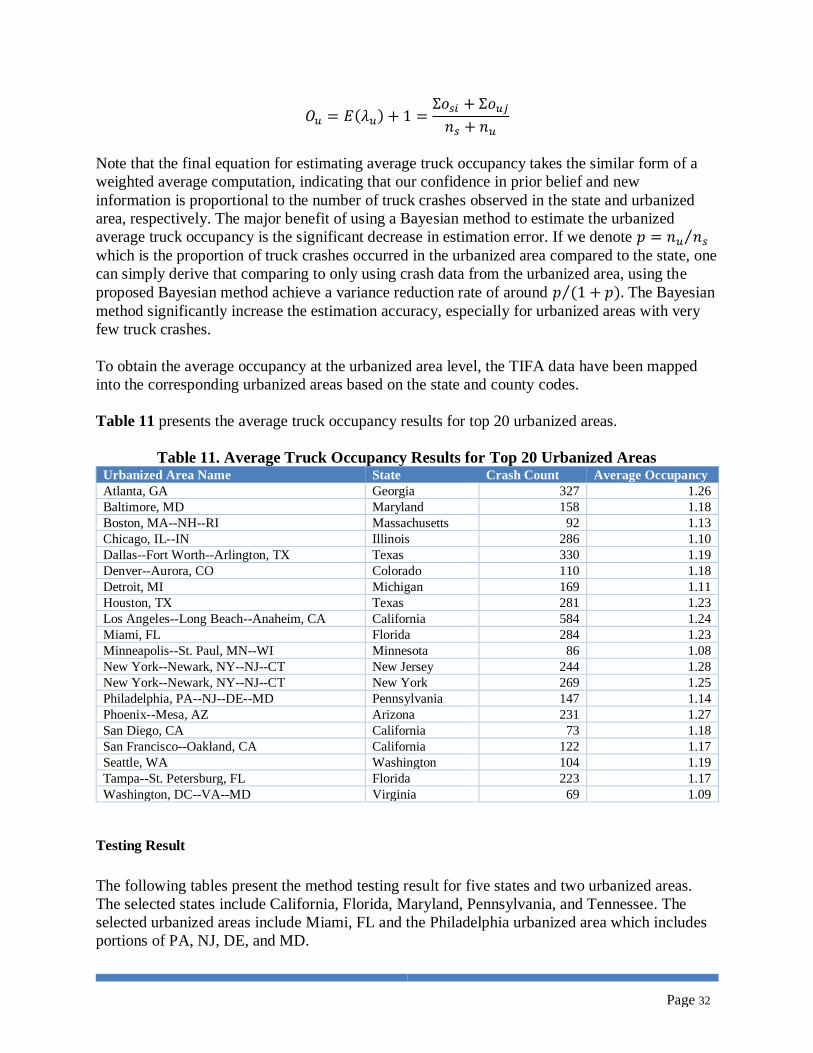
Table 11 presents the average truck occupancy results for top 20 urbanized areas.

Table 11. Average Truck Occupancy Results for Top 20 Urbanized Areas Urbanized Area Name State Crash Count Average Occupancy

Atlanta, GA Georgia 327 1.26

Baltimore, MD Maryland 158 1.18

Boston, MA--NH--RI Massachusetts 92 1.13

Chicago, IL--IN Illinois 286 1.10

Dallas--Fort Worth--Arlington, TX Texas 330 1.19

Denver--Aurora, CO Colorado 110 1.18

Detroit, MI Michigan 169 1.11

Houston, TX Texas 281 1.23

Los Angeles--Long Beach--Anaheim, CA California 584 1.24

Miami, FL Florida 284 1.23

Minneapolis--St. Paul, MN--WI Minnesota 86 1.08

New York--Newark, NY--NJ--CT New Jersey 244 1.28

New York--Newark, NY--NJ--CT New York 269 1.25

Philadelphia, PA--NJ--DE--MD Pennsylvania 147 1.14

Phoenix--Mesa, AZ Arizona 231 1.27

San Diego, CA California 73 1.18

San Francisco--Oakland, CA California 122 1.17

Seattle, WA Washington 104 1.19

Tampa--St. Petersburg, FL Florida 223 1.17

Washington, DC--VA--MD Virginia 69 1.09

Testing Result

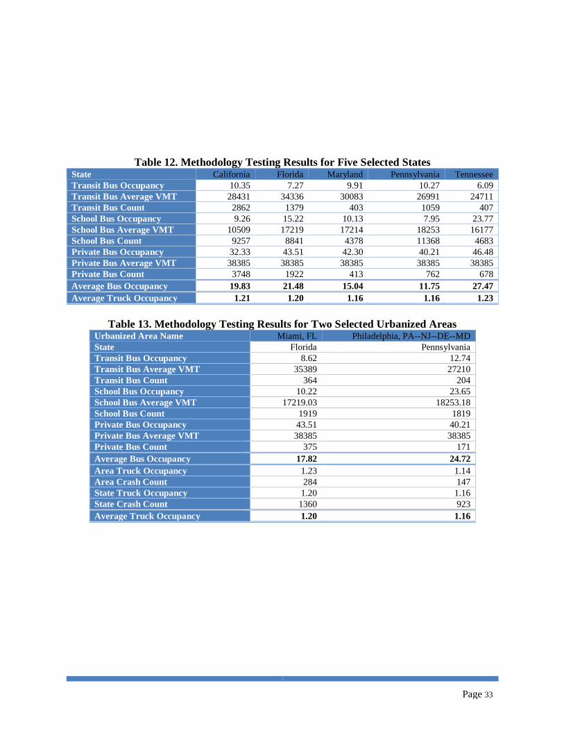
The following tables present the method testing result for five states and two urbanized areas.

The selected states include California, Florida, Maryland, Pennsylvania, and Tennessee. The

selected urbanized areas include Miami, FL and the Philadelphia urbanized area which includes

portions of PA, NJ, DE, and MD.

Page 33

Table 12. Methodology Testing Results for Five Selected States State California Florida Maryland Pennsylvania Tennessee

Transit Bus Occupancy 10.35 7.27 9.91 10.27 6.09

Transit Bus Average VMT 28431 34336 30083 26991 24711

Transit Bus Count 2862 1379 403 1059 407

School Bus Occupancy 9.26 15.22 10.13 7.95 23.77

School Bus Average VMT 10509 17219 17214 18253 16177

School Bus Count 9257 8841 4378 11368 4683

Private Bus Occupancy 32.33 43.51 42.30 40.21 46.48

Private Bus Average VMT 38385 38385 38385 38385 38385

Private Bus Count 3748 1922 413 762 678

Average Bus Occupancy 19.83 21.48 15.04 11.75 27.47

Average Truck Occupancy 1.21 1.20 1.16 1.16 1.23

Table 13. Methodology Testing Results for Two Selected Urbanized Areas Urbanized Area Name Miami, FL Philadelphia, PA--NJ--DE--MD

State Florida Pennsylvania

Transit Bus Occupancy 8.62 12.74

Transit Bus Average VMT 35389 27210

Transit Bus Count 364 204

School Bus Occupancy 10.22 23.65

School Bus Average VMT 17219.03 18253.18

School Bus Count 1919 1819

Private Bus Occupancy 43.51 40.21

Private Bus Average VMT 38385 38385

Private Bus Count 375 171

Average Bus Occupancy 17.82 24.72

Area Truck Occupancy 1.23 1.14

Area Crash Count 284 147

State Truck Occupancy 1.20 1.16

State Crash Count 1360 923

Average Truck Occupancy 1.20 1.16

Page 34

References

American Bus Association. (2017). Motorcoach Census Report: A Study of the Size and Activity

of the Motorcoach Industry in the United States and Canada in 2015.

https://www.buses.org/assets/images/uploads/pdf/Motorcoach_Census_2015.pdf

American School Bus Council. (2015). Environmental Benefits - Fact: You can Go Green by

Riding Yellow. http://www.americanschoolbuscouncil.org/issues/environmental-benefits

Armstrong Atlantic State University. (2013). Motorcoach Tourism in Savannah.

http://www.savannahga.gov/DocumentCenter/View/4364/FINAL-

CoachStudy_AASU_031213?bidId=

Bureau of Economic Analysis (BEA). Regional Data: GDP & Personal Income.

https://apps.bea.gov/itable/iTable.cfm?ReqID=70&step=1#reqid=70&step=1&isuri=1.

Accessed 10/15/2018.

Federal Highway Administration. (2017). Requirement to estimate vehicle occupancy for cars,

buses, and trucks. https://www.gpo.gov/fdsys/pkg/FR-2017-01-18

Gan, A., Jung, R., Liu, K., Li, X., & Sandoval, D. (2005). Vehicle occupancy data collection

methods.

Gan, A., Liu, K., Shen, L., & Jung, R. (2008). Prototype information system for estimating

average vehicle occupancies from traffic accident records. Transportation Research Record:

Journal of the Transportation Research Board, (2049), 29-37.

Hao, X. L., Chen, H. J., Yang, Y. Y., Yao, C., Yang, H., & Yang, N. (2011). Occupant detection

through near-infrared imaging. Tamkang Journal of Science and Engineering, 14(3), 275–

283.

Heidtman, K., Skarpness, B., & Tornow, C. (1997). Improved vehicle occupancy data collection

methods (No. FHWA-PL-98-042,). Office of Highway Information Management, FHWA.

Jarossi, L., Hershberger D. & Woodrooffe J. (2012). Trucks Involved in Fatal Accidents

Codebook 2010. Center for National Truck and Bus Statistics.

Jung, R., & Gan, A. (2010). Sampling and analysis methods for estimation of average vehicle

occupancies. Journal of transportation engineering, 137(8), 537-546.

MAG. (2013). MAG 2012 Vehicle Occupancy Study: Final Report. Maricopa Association of

Governments, Phoenix, Arizona.

New York MTC. (2006). The Vehicle Classification and Occupancy report for 2006.

https://www.nymtc.org/Utility-Menu/Archive/DATA-MODELING-ARCHIVE/VCOS

Mittal, S., Dai, H., Fujimori, S., Hanaoka, T., Zhang, R. (2017). Key factors influencing the

global passenger transport dynamics using the AIM/transport model. Transportation

Research Part D, Vol. 55, pp. 373-388.

Polk City Directory. (2018). Automobile Data. https://www.polkcitydirectories.com/automobile-

data/

U.S. Census Bureau. (2012). 2010 Census Urban and Rural Classification and Urban Area

Criteria. https://www.census.gov/geo/reference/ua/urban-rural-2010.html

Page 35

U.S. Census Bureau. (2018). State Population Totals and Components of Change: 2010-2017.

https://www.census.gov/data/tables/2017/demo/popest/state-total.html. Accessed 10/15/2018

U.S. Census Bureau. (2010). Download Urban Area Relationship Files.

https://www.census.gov/geo/maps-data/data/ua_rel_download.html

U.S. Department of Energy. (2015). Maps and Data - Average Annual Vehicle Miles Traveled of

Major Vehicle Categories. https://www.afdc.energy.gov/data/10309