Embed Size (px)
Citation preview

Deterministic States - Chapter 3 of Heinz
Mathematical Modeling, Spring 2019Dr. Doreen De Leon
1 Introduction
In the process of constructing a model, we need to identify and classify the variables thatinfluence the behavior of the physical system. We must then determine appropriate rela-tionships between those variables that we retain for incorporation into the model. In somesituations, the discovery of the nature of the relationship between independent variables anddependent variables comes about by making some reasonable assumption based on a law ofnature or on previous experience and construction of a mathematical model. In some cases,a series of experiments might be conducted to determine how the variables are related. Aswe have seen, this might result in a figure or a table, and then we may apply an appropriatecurve-fitting method to predict the value of the dependent variable.
Most of our work to this point has focused on modeling observations that were dependent onone variable. In reality, of course, most real-world problems are characterized by relationsinvolving several variables. Dimensional analysis is a method for helping to determine howthe selected variables are related and for significantly reducing the amount of experimentaldata that must be collected. It is based on the premise that physical quantities have di-mensions and that physical laws are not altered by changing the units measuring dimension.Thus, the phenomenon under investigation can be described by a dimensionally consistentrelation among the variables. A dimensional analysis provides qualitative information aboutthe model. It is especially important when it is necessary to conduct experiments as partof the modeling process, because the method is helpful in testing the validity of includingor neglecting a particular factor; in reducing the number of experiments that need to beconducted to make predictions; and in improving the usefulness of the results by providingalternatives for the parameters employed to present them.
Although dimensional analysis is very useful for validating newly developed mathematicalmodels or for confirming that certain formulas makes sense, applying the tools of dimen-sional analysis does not always yield desirable results. In addition, equations derived usingdimensional analysis will still have unknowns for which we must solve.
1

2 Modeling Using Geometric Similarity
Geometric similarity is a concept that you should have encountered in multiple math courses,such as geometry (in middle or high school) and calculus. It is another tool that can be usedto simplify the mathematical modeling process.
Definition 2.1. Two objects are geometrically similar if there is a one-to-one correspondencebetween points of the objects, such that the ratio of the distances between correspondingpoints is constant for all pairs of points.
Examples include: similar triangles and the use of scaling on a map.
We will look at an example of modeling with geometric similarity before we begin ourdiscussion of dimensional analysis.
One advantage of two objects being geometrically similar is a simplification in some compu-tations, such as volume and surface area. Suppose that we have two similar boxes, a smallerbox with dimension l1, w1, h1 and a larger box of dimensions l2, w2, h2. Then, the ratio oftheir volumes is given by
V1V2
=l1w1h1l2w2h2
= k3,
since l2 = kl1, w2 = kw1, h2 = kh1. Similarly, the ratio of the total surface areas is given by
S1
S2
=2l1h1 + 2w1h1 + 2w1l12l2h2 + 2w2h2 + 2w2l2
= k2.
Note also that the surface area and volume may be expressed as a proportionality in termsof a chosen dimension, the characteristic dimension. Suppose we choose the length as thecharacteristic dimension. Then
S1
S2
= k2 =l21l22.
Or, we can say thatS1
l21=S2
l22= constant
holds for any two geometrically similar objects; i.e., S ∝ l2. Similarly, we can show thatvolume is proportional to the cube of the length, or V ∝ l3.
Example 2.1 (Raindrops from a Motionless Cloud). Suppose we wish to determine theterminal velocity of a raindrop from a motionless cloud. If we draw a free body diagram, wewill see that the only forces acting on the raindrop are gravity and air resistance, or drag.We will make the following assumptions:
• atmospheric drag on the raindrop is proportional to the product of the drop’s surfacearea S and the square of its velocity v;
2

• the weight of the raindrop w is proportional to its mass m (assuming constant gravity);and
• all raindrops are geometrically similar.
By Newton’s second law, F = Fg−Fd = ma, and under terminal velocity a = 0, so Newton’ssecond law is reduced to
Fg − Fd = 0,
orFg = Fd.
Assuming that Fd ∝ Sv2 and the force of gravity is proportional to the weight w, Fg ∝ w.Since m ∝ w, we have Fg ∝ m. Assuming that all raindrops are similar, we can relatesurface area and volume. Since
S ∝ l2 and V ∝ l3,
where l is the characteristic dimension, it follows that
l ∝ S12 ∝ V
13 .
Therefore,S ∝ V
23 .
Since weight and mass are proportional to volume, applying the transitive rule for propor-tionality gives
S ∝ m23 .
Since Fg = Fd, we have that
m ∝ m23v2,
orv ∝ m
16 .
3 Dimensional Analysis and Similarity - Section 3.2 of
Heinz
3.1 Dimensions as Products
The study of physics is based on concepts such as mass, length, time, velocity, acceleration,force, energy, work, and pressure. To each such concept, a unit of measurement is assigned.A physical law, such as Newton’s law, is true, provided that the units of measurement areconsistent. Thus, if mass is measured in kilograms and acceleration in meters per second
3

squared, then the force must be measured in Newtons. These units of measure belong to theMKS (meter-kilogram-second) system. In the English system, mass is in slugs, accelerationis in feet per second squared, and force is in pounds.
The three primary physical quantities that we will consider in this section are mass, length,and time. We associate with these quantities the dimensions M, L, and T, respectively. Thedimensions are symbols that reveal how the numerical value of a quantity changes when theunits of measurement change in certain ways. The dimensions of other quantities follow fromdefinitions or from physical laws and are expressed in terms of M, L, and T. For example,acceleration is represented as LT−2. There are other, more complicated physical quantitiesthat are not usually defined directly in terms of mass, length, and time, but in terms of otherquantities, such as velocity. For example, momentum is the product of mass and velocity.Thus, its dimension is MLT−1.
The basic definition of a quantity may also involve dimensionless constants, which are ignoredin finding the dimension. Thus, the dimension of kinetic energy, which is one half the product
of the mass and the velocity squared, is M(LT−1
)2= ML2T−2.
Quick recap so far:
1. The concept of dimension is based on three physical quantities, mass, length, and time.These quantities are measured in some appropriate system of units whose choice doesnot affect the assignment of dimensions.
2. There are other physical quantities, such as area and velocity, that are defined as simpleproducts involving only mass, length, or time.
3. There are other, more complex physical properties, such as energy, whose definitionsinvolve quantities other than mass, length, and time, but which we may use definitionsand physical laws to write as products only involving mass, length, and/or time.
4. To each product, there is assigned a dimension, i.e., an expression of the form
MnLpT q, (3.1)
where n, p, and q are real numbers.
When a basic dimension is missing from a product, the corresponding exponent is understoodto be 0. When n, p, and q are all zero in an expression of the form (3.1), so that the dimensionreduces to
M0L0T 0,
the quantity is said to be dimensionless.
One must be careful in forming sums of products, because we cannot add products that haveunlike dimensions.
4

Another important concept is that of dimensional homogeneity. In general, an equationthat is true regardless of the system of units in which the variables are measured is said tobe dimensionally homogeneous. For example, the equation giving the time a body falls adistance s under gravity (neglecting air ressistance) is
t =
√2s
g.
This expression is dimensionally homogeneous.
Example 3.1 (Simple Pendulum). Consider a simple pendulum of length r, which has amass m attached to it. Let θ denote the initial angle of displacement from the vertical.One characteristic of interest is the period (the time required for the pendulum to swingthrough one complete cycle, returning to its starting point). We represent the period of thependulum as t. We will analyze this problem using dimensional analysis, under the followingassumptions:
• the hinge is frictionless;
• the mass is concentrated at one end of the pendulum; and
• the drag force is negligible.
First, analyze the dimensions of the variables.
Variable m g t r θ
Dimension M LT−2 T L M0L0T 0
Next, find all of the dimensionless products among the variables. Any such product musttake the form
magbtcrdθe, (3.2)
and therefore, must have dimension
(M)a(LT−2)b(T )c(L)d(M0L0T 0)e = MaLb+dT c−2b. (3.3)
Therefore, a product of the form (3.2) is dimensionless if and only if
MaLb+dT c−2b = M0L0T 0.
This gives the linear system of equations
a = 0b + d = 0
−2b + c = 0.
We can see that there are infinitely many solutions. The rules for choosing arbitrary variableswhen doing dimensional analysis are the following.
5

(1) Choose the dependent variable so it will only appear once.
(2) Select any variable that will speed up the solving of the system; e.g., choose a variablethat appears in all (or most) equations.
With that in mind, we should choose b as the independent variable, and therefore, thesolution to the system is
a = 0; c = 2b; d = −b.The other independent variable is e, because it does not appear in the system.
One dimensionless product is obtained by setting b = 0 and e = 1, giving a = c = d = 0.A second dimensionless product is obtained by setting b = 1 and e = 0, giving a = 0, c =2, and d = −1. These solutions give the dimensionless products
Π1 = m0g0t0r0θ1 = θ
Π2 = m0g1t2r−1θ0 =gt2
r.
Assuming that t = f(r,m, g, θ), we need to determine more about the function f . First, ifthe units of m were to change by some factor, the measure of the period will not change,because it is measured in units (T ) of time. Also note that because m is the only factorwhose dimension contains M , it cannot appear in the model. If the scale of the units (L) formeasuring length were changed, then it also can’t change the measure of the period, either.In order to ensure that this is correct, then g and r must appear together in the model as
some power ofg
r. Finally, if we make the units (T ) that measure time smaller by a factor
of, say, 10, then the measure of the period will increase by this same factor. Therefore, to
have the dimension of T on the right-hand side of t = f(r,m, g, θ), r must appear as
√r
g,
because T appears to the power of -2 in the dimension of g. Note that we have not foundanything to restrict the angle θ. Therefore, the equation for the period should take the form
t =
√r
gh(θ),
where h is a function to be determined or approximated experimentally.
Question: Is it reasonable to assume that the friction and drag forces are negligible?
Answer: The model obtained so far is
t =√rgh(θ).
If θ is kept constant, say θ = θ0, while r is allowed to vary, we have
t1t2
=
√r1/gh(θ0)√r2/gh(θ0)
=
√r1r2.
6
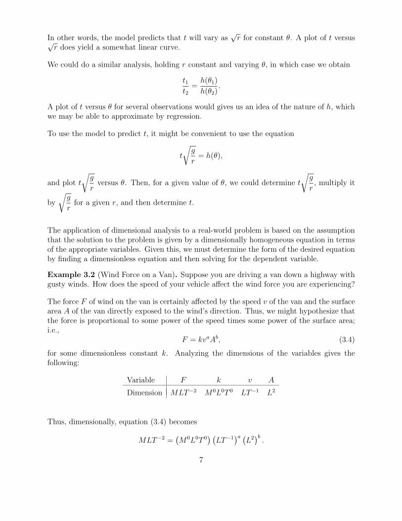
In other words, the model predicts that t will vary as√r for constant θ. A plot of t versus√
r does yield a somewhat linear curve.
We could do a similar analysis, holding r constant and varying θ, in which case we obtain
t1t2
=h(θ1)
h(θ2).
A plot of t versus θ for several observations would gives us an idea of the nature of h, whichwe may be able to approximate by regression.
To use the model to predict t, it might be convenient to use the equation
t
√g
r= h(θ),
and plot t
√g
rversus θ. Then, for a given value of θ, we could determine t
√g
r, multiply it
by
√g
rfor a given r, and then determine t.
The application of dimensional analysis to a real-world problem is based on the assumptionthat the solution to the problem is given by a dimensionally homogeneous equation in termsof the appropriate variables. Given this, we must determine the form of the desired equationby finding a dimensionless equation and then solving for the dependent variable.
Example 3.2 (Wind Force on a Van). Suppose you are driving a van down a highway withgusty winds. How does the speed of your vehicle affect the wind force you are experiencing?
The force F of wind on the van is certainly affected by the speed v of the van and the surfacearea A of the van directly exposed to the wind’s direction. Thus, we might hypothesize thatthe force is proportional to some power of the speed times some power of the surface area;i.e.,
F = kvaAb, (3.4)
for some dimensionless constant k. Analyzing the dimensions of the variables gives thefollowing:
Variable F k v A
Dimension MLT−2 M0L0T 0 LT−1 L2
Thus, dimensionally, equation (3.4) becomes
MLT−2 =(M0L0T 0
) (LT−1
)a (L2)b.
7

Obviously there is something wrong here, because the dimension M for mass does not appearon the right-hand side.
So, we must revise equation (3.4). What is missing from our original assumptions regardingthe factors that affect the wind force on the van? After some reflection, we might considerthat density ρ has an effect. Including density as a factor makes the model
F = kvaAbρc. (3.5)
Since density is mass per unit volume, the dimension of density is ML−3. Thus, dimension-ally, equation (3.5) is
MLT−2 =(M0L0T 0
) (LT−1
)a (L2)b (
ML−3)c.
Equating exponents on both sides of the equation gives the system of equations
c = 1a + 2b − 3c = 1−a = −2
,
whose solution is a = 2, b = 1, and c = 1. Thus, the model is
F = kv2Aρ.
Table 3.1 gives a summary of the dimensions of some common physical quantities.
Table 3.1: Dimensions of physical quantities
Mass M Momentum MLT−1
Length L Work ML2T−2
Time T Density ML−3
Velocity LT−1 Viscosity ML−1T−1
Acceleration LT−2 Pressure ML−1T−2
Specific weight ML−2T−2 Surface tension MT−2
Force MLT−2 Power ML2T−3
Frequency T−1 Rotational inertia ML2
Angular velocity T−1 Torque ML2T−2
Angular acceleration T−2 Entropy ML2T−2
Angular momentum ML2T−1 Heat ML2T−2
Energy ML2T−2
8

3.2 The Process of Dimensional Analysis
Our goal now is to investigate how to use dimensionless products to find all possible dimen-sionally homogeneous equations among the variables. The key result is Buckingham’s PiTheorem, which summarizes the theory of dimensional analysis.1
The theorem loosely states that if we have a physically meaningful equation involving acertain number, say n, of physical variables, and those variables are expressed in terms of mfundamental (or primary) physical quantities, then the original expression is equivalent to anequation involving n−m dimensionless variables constructed from the original variables. Thisprovides a method for computing sets of dimensionless parameters from the given variables,even if the form of the equation is still unknown. However, the choice of dimensionlessparameters is not unique; Buckingham’s theorem only provides a way of generating sets ofdimensionless parameters, and will not choose the most “physically meaningful.”
In mathematical terms, if we have a physically meaningful equation, such as
f(q1, q2, . . . , qn) = 0,
where the qi are n physical variables, and they are expressed in terms of m independentphysical units, then the above equation can be restated as
φ(Πi,Π2, . . . ,Πn−m) = 0,
where the Πi are dimensionless parameters constructed from the qi by n −m equations ofthe form
Πi = qm11 qm2
2 · · · qmnn ,
where the exponents mi are rational numbers. The use of Πi to represent the dimensionlessparameters was introduced by Edgar Buckingham in his original 1914 paper On physicallysimilar systems; illustrations of the use of dimensional equations, in Physical Review, 4, pp.345–376.
Formal statement of the theorem:
Theorem 3.1 (Buckingham’s Pi Theorem). Any physically meaningful relation
F (Q1, Q2, . . . , Qn) = 0,
where Qi are n physical variables such that Qi 6= 0 and the Qi are expressed in terms of mindependent physical units, is equivalent to a relation of the form
ψ(Π1,Π2, . . . ,Πn−m) = 0,
1A portion of this discussion is taken from Principles of Mathematical Modeling, second edition, by CliveL. Dym and a Wikipedia entry on Buckingham’s Pi Ttheorem.
9

where Πi are dimensionless parameters constructed from the Qi by n −m equations of theform
Πi = Qm11 Qm2
2 · · ·Qmnn ,
where mi ∈ Q.
Alternately, the relation can be written in the form
Π1 = φ(Π2,Π3, . . . ,Πn−m).
3.3 Similarity
Suppose that we are interested in the effects of wave action on a large ship at sea, heat loss of asubmarine and the drag force it experiences in its underwater environment, or the wind effectson an aircraft wing. Frequently, we study a scaled-down model in a simulated environmentto predict accurately the performance of the physical system. The actual physical systemfor which the predictions are to be made is called the prototype. The question is: How dowe scale experiments in the laboratory to ensure that the effects observed for the model willbe the same as those experienced by the prototype?
The dimensional products resulting from dimensional analysis of the problem can provideinsight into how the scaling for a model should be done. The idea comes from Buckingham’sPi Theorem. If the physical system can be described by a dimensionally homogeneousequation in n variables, then it can be put into the form
ψ (Π1,Π2, . . . ,Πp) = 0
for a set of p dimensionless products (where p = n−m, m being the number of independentphysical units). Assume that the dependent variable of the problem appears only in theproduct Πp and that
Πp = φ (Π1,Π2, . . . ,Πp−1) .
For the solution to the model and the prototype to be the same, it is sufficient that the valueof all independent dimensionless products Π1,Π2, . . . ,Πp−1 be the same for both the modeland the prototype.
For example, suppose the Reynold’s numbervrρ
µappears as one of the dimensionless prod-
ucts in a fluid mechanics problem, where v represents the fluid velocity, r is a characteristicdimension, such as the length of a ship, ρ represents the fluid density, and µ represents thefluid viscosity. Then, let vm, rm, ρm, and µm be the values for the scaled model. For theeffects on both the prototype and the model to be the same, we need
vrρ
µ=vmrmρmµm
.
10

This equation is known as a design condition to be satisfied by the model. For example, ifwe need to scale the length of the prototype by a factor of 10 (so, r = 10rm), then the sameReynold’s number can be obtained by using the same fluid (so ρm = ρ and µm = µ) andchanging the velocity (so vm = 10v). If this is impractical, then a different fluid can be usedso that the equation is satisfied.
4 Examples of Low Complexity - Section 3.3 of Heinz
4.1 Kepler’s Third Law
Our goal is to calculate the orbital period of a planet, TP . On what variables does the orbitalperiod depend?
• (mean) distance from the sun, r;
• gravitational force FG; and
• the mass m of the planet.
Analyzing the dimensions of the variables gives
Variable r FG m TP
Dimension L MLT−2 M T
Next, we must find all dimensionless products among the variables. Any such product mustbe of the form
raF bGm
cT dP ,
and so, must have dimensionLa(MLT−2)bM cT d.
Therefore, the product is dimensionless if and only if
a + b = 0b + c = 0
−2b + d = 0.
This system has infinitely many solutions of the form
a = −bc = −bd = 2b
11

We find Π1 by letting b = 1, giving a = −1, c = −1, d = 2, or
Π1 = r−1Fgm−1T 2
P .
Since there is only one nondimensional product, it must be constant, so we have
r−1Fgm−1T 2
P = c,
where c is a constant, or
TP = c1
√mr
FG
,
where c1 is a nonnegative constant. Since this formula does not rely on the fact that thepaths of the planets are elliptical, we may assume that the planets revolve around the sunin a circular orbit. Applying Newton’s second law, we have
FG = ma = m
(4π2r
T 2P
)= 4π2 rm
T 2P
.
Solving for TP gives
TP = 2π
√mr
FG
,
and so c1 = 2π.
4.2 Drag Force of Object in a Fluid
Our goal is to analyze the drag force of an object moving through a fluid. We make theassumption that the objects are spherical. The motion of the spherical objects is dampedby the surrounding fluid. The relevant variables are
• damping force Fd;
• radius of the sphere r;
• the relative velocity between the sphere and the fluid, v; and
• the fluid viscosity µ.
Analyzing the dimensions of the variables gives
Next, we must find all dimensionless products among the variables. Any such product mustbe of the form
Fm1d rm2vm3µm4 = (MLT−2)m1Lm2(LT−1)m3(ML−1T−1)m4 ,
12

Variable Fd r v µ
Dimension MLT−2 L LT−1 ML−1T−1
and so, must have dimension
Mm1−m4Lm1+m2+m3−m4T−2m1−m3−m4 .
Therefore, the product is dimensionless if and only if
m1 + m4 = 0m1 + m2 + m3 − m4 = 0
−2m1 − m3 − m4 = 0.
1 0 0 1 | 01 1 1 −1 | 0−2 0 −1 −1 | 0
R2−R1→R2−−−−−−−→R3+2R1→R3
1 0 0 1 | 00 1 1 −2 | 00 0 −1 1 | 0
R2+R3→R2−−−−−−−→
1 0 0 1 | 00 1 0 −1 | 00 0 −1 1 | 0
.Therefore, m4 is a free variable, and we may solve for all other variables in terms of m4.Alternately, we may choose m1 to be the free variable (since it appears in each equation, aswell), giving
m4 = −m1
m2 = m4 = −m1
m3 = m4 = −m1.
Let m1 = 1. Then m2 = m3 = m4 = −1, and we have one dimensionless product,
Π1 =Fd
rvµ.
Therefore,Fd
rvµ= c,
where c is a constant, andFd = crvµ.
Other methods may be used to show that c = 6π, so
Fd = 6πrvµ.
13

5 Applications of Medium-Complexity - Section 3.4 of
Heinz
5.1 Terminal Velocity of a Raindrop Revisited
Consider the problem of determining the terminal velocity v of a raindrop falling from amotionless cloud. We have looked at this problem before, taking a simpler view of it. Now,we will look at the problem using dimensional analysis.
First, what are the variables influencing the behavior of the raindrop? Obviously, the termi-nal velocity will depend on the size of the raindrop given by, say, its radius r. The densityρ of the air and the viscosity µ of the air will also affect the behavior (since viscosity mea-sures the resistance to motion, which, in gases, is caused by collisions between fast-movingmolecules). Another important variable is the acceleration due to gravity g. Although thesurface tension of the raindrop is a factor that influences the behavior of the raindrop’sdescent, we will ignore it here. If necessary, surface tension can be taken into account in alater, refined model. Analyzing the dimensions of the variables gives
Variable v r g ρ µ
Dimension LT−1 L LT−2 ML−3 ML−1T−1
Next, we must find all dimensionless products among the variables. Any such product mustbe of the form
varbgcρdµe, (5.1)
and, so, must have dimension(LT−1
)aLb(LT−2
)c (ML−3
)d (ML−1T−1
)e.
Therefore, a product of the form (5.1) is dimensionless if and only if the following system ofequations is satisfied
d + e = 0a + b + c − 3d − e = 0−a − 2c − e = 0
.
The system has infinitely many solutions
b =3
2d− 1
2a
c =1
2d− 1
2a
e = −d,
14

where a and d are arbitrary.
One dimensionless product Π1 is obtained by setting a = 1, d = 0, and another, Π2 isobtained by setting a = 0, d = 1. So,
Π1 = vr−12 g−
12 , and Π2 = r
32 g
12ρµ−1.
You should check the results to verify that the products are dimensionless.
Then, according to Buckingham’s Pi Theorem, there is a function ψ such that
ψ(vr−
12 g−
12 , r
32 g
12ρµ−1
)= 0.
Assuming that we can solve this equation for vr−12 g−
12 as a function of Π2, it follows that
v =√rgφ
(r
32 g
12ρ
µ
),
where φ is some function of Π2.
5.2 A Damped Pendulum
We have already looked at a simple pendulum, in which we ignored the effects of a dragforce and of friction. Now, we will analyze the system, this time incorporating the effects ofdrag on the motion of the pendulum. We continue to assume that the hinge is frictionlessand that the mass is concentrated at the end of the pendulum. Let Fd represent the totaldrag force. Our goal is to determine the period of a pendulum of length r with a mass mattached to it; denote θ as the initial angle of displacement from the vertical.
First, we need to determine a model for the drag force. For our pendulum, it is reasonableto assume that either
• the drag force is proportional to the velocity, v: Fd ∝ v; i.e., Fd = kv; or
• the drag force is proportional to the square of the speed: Fd ∝ v|v|; i.e., Fd = kv|v|(sometimes simply written as Fd = kv2, when we are considering v as speed).
For simplicity, we will assume that Fd = kv. To simplify our analysis, we will use the
dimensional constant k =Fd
v, which has dimension
MLT−2
LT−1= MT−1.
15

Next, analyze the dimensions of the variables.
Variable m g t r θ k
Dimension M LT−2 T L M0L0T 0 MT−1
Then, find all of the dimensionless products among the variables. Any such product musttake the form
magbtcrdθekf , (5.2)
and therefore, must have dimension
(M)a(LT−2)b(T )c(L)d(M0L0T 0)e(MT−1)f = Ma+fLb+dT c−2b−f . (5.3)
Therefore, the product (5.2) is dimensionless if and only if
a + f = 0b + d = 0
−2b + c − f = 0.
We have three equations in six unknowns, and we would like to choose solutions so that tappears in only one of the dimensionless products. So, we choose c, e, and f as the arbitraryvariables, giving the solutions
a = −f
b =1
2(c− f)
d = −b.
Setting c = 1, e = f = 0, we obtain a = 0, b =1
2, d = −1
2. Setting e = 1, c = f = 0, we
obtain a = b = d = 0. And, setting c = e = 0, f = 1, we obtain a = −1, b = −1
2, d =
1
2.
Therefore, we have the following dimensionless products.
Π1 = g12 tr−
12 .
Π2 = θ, and
Π3 = m−1g−12 r
12k.
From Buckingham’s Pi Theorem, there is a function ψ such that
ψ
(t
√g
r, θ,
k
m
√r
g
)= 0.
16

Assuming that we can solve this equation for t
√g
r, we obtain
t =
√r
gφ
(θ,k
m
√r
g
),
where φ is some function of Π2 and Π3.
To test the model, we could do something similar to what we discussed in Example 3.1, butthis would be somewhat problematic, since our goal is to hold parameters of the functionφ constant, while varying other parameters. In this case, however, we cannot vary r whilekeeping Π3 constant. We can, however, try to vary r so that
√r/m stays constant.
To use the model in a predictive sense, one could plot t
√g
rversus
k
m
√r
gfor various values
of θ. To be effective, this would require several trials with various values ofk
m
√r
g. Once
the data is obtained, a model can be determined using regression.
Choosing Among Competing Models
Since dimensional analysis only involves algebra, as opposed to application of physical prin-ciples, it might be a good idea to develop multiple models under different assumptions beforeperforming experiments, which could potentially be very costly. There are three models wecan look at for the pendulum problem:
(1) no drag forces: t =
√r
gh(θ);
(2) drag force proportional to v: t =
√r
gφ
(θ,k
m
√r
g
); and
(3) drag force proportional to v2: t =
√r
gφ
(θ,k1r
m
).
Experimentation would indicate which model is best under different circumstances.
17

6 Applications of High-Complexity - Section 3.5 of Heinz
6.1 Draining Cylinder
Consider a right cylinder of cross-sectional area A filled to depth H with a perfect liquid ofdensity ρ. A hole of area a is made in the bottom of the container, and the liquid drainsunder the influence of gravity with acceleration g.2 Determine T , the time for the containerto empty, in terms of the parameters A,H, ρ, a, and g. Analyzing the dimensions of thevariables gives
Variable T A H ρ a g
Dimension T L2 L ML−3 L2 LT−2
Next, we must find all dimensionless products among the variables. Any such product mustbe of the form
Tm1Am2Hm3ρm4am5gm6 , (6.1)
and, so, must have dimension
Tm1(L2)m2 Lm3
(ML−3
)m4(L2)m5
(LT−2
)m6 .
Therefore, a product of the form (5.1) is dimensionless if and only if the following system ofequations is satisfied
m1 − 2m6 = 0m4 = 0
2m2 + m3 − 3m4 + 2m5 + m6 = 0.
Clearly, this system has infinitely many solutions, with m4 = 0
m1 = 2m6
m3 = −2m2 − 2m5 −m6
Find Π1 by letting m6 = 1,m2 = 0,m5 = 0 to obtain m1 = 2 and m3 = −1. Find Π2 byletting m6 = 0,m2 = 1, and m5 = 0 to obtain m1 = 0 and m3 = −2. Finally, find Π3 byletting m6 = 0,m2 = −1, and m5 = 1 to obtain m1 = 0 and m3 = 0. Our dimensionlessconstants are then
Π1 = T 2H−1g
Π2 = AH−2
Π3 = A−1a
2This example is adapted from James Graham-Eagle’s paper, The Draining Cylinder in the The CollegeMathematics Journal, Volume 40, Number 5, November 2009, pp. 337–343
18

Therefore, according to Buckingham’s Pi Theorem, there is a function ψ such that
ψ(T 2H−1g, AH−2, A−1a
)= 0.
If we assume that we can solve for T 2H−1g, we will obtain a function of the form
T =
√H
gφ
(A
H2,a
A
).
Let us see if we can work towards determining an exact expression. Suppose that both Aand a are scaled by the same value β. It seems reasonable that T is not affected by thischange. This implies that
T =
√H
gφ
(βA
H2,βa
βA
)=
√H
gφ
(βA
H2,a
A
).
This demonstrates that φ(x, y) is independent of x, so we now have
T =
√H
gφ( aA
).
Can we do better? Consider the evolution of the system as a function of time. Since thevolume in the cylinder is Ah, where h represents the height of the fluid at any time, the rate
at which the volume decreases is −d(Ah)
dt. This equals the rate at which the liquid drains
from the hole in the bottom of the container, av, where v is the speed at which the liquidflows from the hole. Since A is constant, equating the two quantities yields the differentialequation
Adh
dt= −av.
If we assume that v depends only on h and g, which seems reasonable since the pressure atthe bottom of the container is what drives the liquid through the hole, and pressure dependson h and g, then the differential equation is separable and may be solved by integrating bothsides over the duration of the experiment.∫ 0
H
1
vdh =
∫ T
0
− aAdt
=⇒∫ H
0
1
vdh =
a
AT
=a
A
√H
gφ( aA
).
19

Differentiating the above equation with respect to H gives
1
v(H)=
1
2√gH
a
Aφ( aA
).
Since v does not depend on a or A, it follows that φ(x) =C
xfor some constant C. So, we
now have that
T =
√H
gCA
a.
Now, if a = A, then the entire base of the container is gone and the liquid falls as a rigidbody under the influence of gravity. Since, in evacuating the container, the liquid falls adistance H from rest, it follows that
T =
√2H
gwhen a = A.
Thus, C =√
2, and we obtain
T =A
a
√2H
g,
or Torricelli’s law.
Note: Typically, Torricelli’s law appears as a problem in Calculus and differential equationstextbooks. The standard solution approach involves equating the rate of loss of water inthe container with the rate at which it passes through the hole, applying Torricelli’s lawto determine the latter expression. For our problem involving a right circular cylinder, thisreduces to solving the separable first order equation
Adh
dt= −a
√2gh.
6.2 Explosion Analysis
In excavating and mining operations, it is obviously very important to be able to predictthe size of an explosion resulting from the use of TNT (or some other explosive agent) ina given type of soil. Since direct experimentation is expensive (and destructive), we wouldlike to be able to use small laboratory or field tests and then use scaling to determine effectsof explosions of greater magnitude.
Step 1: Identify the Problem. Predict the volume of the crater formed by a sphericalexplosive placed at a depth d below the surface of the soil.
Step 2: Make Simplifying Assumptions. Initially, our assumptions will be as follows.
20

• The explosive is spherical.
• The craters are geometrically similar.
• The crater size depends on the following variables:
– the radius r of the crater;
– the density ρ of the soil; and
– the mass m of the explosive.
Step 3: Construct the Model. We apply dimensional analysis, using the above assumptions.We search for all dimensionless products among the three variables. Any such product hasthe form
rm1ρm2mm3 ,
which has dimensionMm2+m3Lm1−3m2 .
A product of this form is dimensionless if and only if
m1 − 3m2 = 0m2 + m3 = 0
.
Since we are interested in solving for the radius, we will let m1 be the free variable, and setm1 = 1. Then
m2 =1
3and m3 = −1
3.
Therefore, we obtain one dimensionless product,
Π1 = r( ρm
) 13.
Since there is only one dimensionless product, it must be a constant, giving
r( ρm
) 13
= c,
or
r = c
(m
ρ
) 13
.
Step 4: Solve and Interpret the Model. Therefore, the crater dimension of the radius varieswith the cube root of the mass of the explosive. Since the crater volume is proportional tor3, the volume of the crater will thus be proportional to m/ρ, or
V ∝ m
ρ.
21

Step 5: Validate the Model. It has been shown experimentally that this is an adequatemodel for small explosions (less than 300 lb. of TNT) at zero depth in the soils that havegood cohesion. For larger explosions, though, this model is unsatisfactory.
Since the model is not good for larger explosions, we must re-evaluate the model, incorpo-rating more (or different) variables.
Assumptions: Suppose that we now take into account gravity and the charge energy E ofthe explosive. The charge energy is defined as the product of the mass of the explosive Wand its specific energy. We apply dimensional analysis again, searching for all dimensionlessproducts among the variables r, ρ, g, and E, i.e., for dimensionless products of the form
rm1ρm2gm3Em4 .
Analyzing the dimensions of the variables, we see that So, any dimensionless product must
Variable r ρ g EDimension L ML−3 LT−2 ML2T−2
have dimension
Lm1(ML−3)m2(LT−2)m3(ML2T−2)m4 = Mm2+m4Lm1−3m2+m3+2m4T−2m3−2m4 .
For the product to be dimensionless, the linear system
m1 − 3m2 + m3 + 2m4 = 0m2 + m4 = 0
−2m3 − 2m4 = 0.
Solve this system.1 −3 1 2 | 00 1 0 1 | 00 0 −2 −2 | 0
R1+3R2→R1−−−−−−−→
1 0 1 5 | 00 1 0 1 | 00 0 −2 −2 | 0
− 12R2→R2−−−−−−→
1 0 1 5 | 00 1 0 1 | 00 0 1 1 | 0
R1−R3→R1−−−−−−−→
1 0 0 4 | 00 1 0 1 | 00 0 1 1 | 0
Again, we may let m1 be the free variable since we wish to solve for r. So, let m1 = 1. Then
m4 = −1
4,m2 = m3 =
1
4.
Thus, we obtain one dimensionless constant, which will be constant, or
r(ρgE
) 14
= c,
22

giving
r = c
(E
ρg
) 14
.
Therefore, we have that
V ∝(E
ρg
) 34
. (6.2)
Experimental evidence indicates that scaling based on gravity holds for large explosion (morethan 100 tons of TNT) where the stresses caused by the explosion are much larger than thematerial strength of the soil. The model (6.2) predicts that the volume of the crater willdecrease as gravity increases. This obviously has relevance in the context of craters formedon other planets (or moons).
6.2.1 More Complex Explosive Models
We can arrive at more complicated models by considering the question of whether or not thematerial properties of the soil play a less significant role as the size of the charge increasesand as gravity increases. To simplify this question, we assume that the only soil property ofinterest is the density ρ. (Note that this is what we have already done, so we are not addinganything in this area.) We will also fine-tune the model, using more detail to describe itthan we previously did.
Three variables are required to characterize an explosive:
• the size of the explosive, which can be described in terms of the charge mass W , thecharge energy E, or the radius α of the spherical explosive;
• the energy yield, which can be measured by the specific energy, Qe or the energydensity per unit volume, QV ; and
• the explosive density δ.
The variables can be related by the following equations:
W =E
Qe
QV = δQe
αe =
(3
4π
)(W
δ
).
23

We may, therefore, select a subset of the variables for our model formulation. UsingV,W,Qe, δ, ρ, g, and d, we may search for all dimensionless products. Such products havethe form
V m1Wm2Qm3e δm4ρm5gm6dm7 .
Analyzing the dimensions of the variables, we see that
Variable V W Qe δ ρ g dDimension L3 M L2T−2 ML−3 ML−3 LT−2 L
So, any dimensionless product must have dimension
(L3)m1Mm2(L2T−2)m3(ML−3)m4(ML−3)m5(LT−2)m6Lm7 ,
orL3m1+2m3−3m4−3m5+m6+m7Mm2+m4+m5T−2m3−2m6 .
Such a product is dimensionless if
3m1 + 2m3 − 3m4 − 3m5 + m6 + m7 = 0m2 + m4 + m5 = 0
−2m3 − 2m6 = 0.
Applying Gaussian elimination gives3 0 2 −3 −3 1 1 | 00 1 0 1 1 0 0 | 00 0 −2 0 0 −2 0 | 0
R1+R2→R1−−−−−−−→
3 0 2 −3 −3 −1 1 | 00 1 0 1 1 0 0 | 00 0 −2 0 0 −2 0 | 0
.Since we had three equations in seven unknowns, we expected that we would have four freevariables. We may choose m1 (since we wish to solve for the volume) and three other variablesas the free variables. If we choose m5,m6, and m7 (as we would do in a linear algebra class),we obtain the dimensionless products by finding a basis for the solution space. Since solvinggives
m2 =1
3(m7 −m6)−m1
m3 = −m6
m4 = m1 −m5 +1
3(m6 −m7),
setting each free variable equal to 1 and the other three equal to 0 gives the following
24
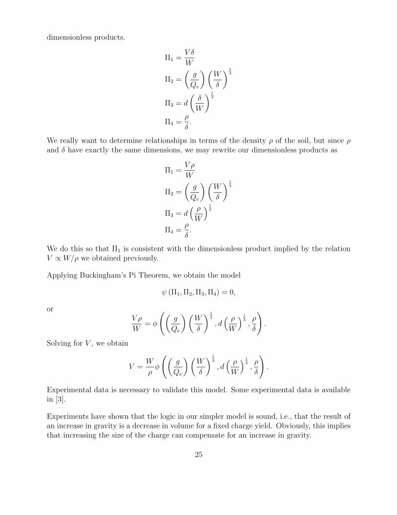
dimensionless products.
Π1 =V δ
W
Π2 =
(g
Qe
)(W
δ
) 13
Π3 = d
(δ
W
) 13
Π4 =ρ
δ.
We really want to determine relationships in terms of the density ρ of the soil, but since ρand δ have exactly the same dimensions, we may rewrite our dimensionless products as
Π1 =V ρ
W
Π2 =
(g
Qe
)(W
δ
) 13
Π3 = d( ρW
) 13
Π4 =ρ
δ.
We do this so that Π1 is consistent with the dimensionless product implied by the relationV ∝ W/ρ we obtained previously.
Applying Buckingham’s Pi Theorem, we obtain the model
ψ (Π1,Π2,Π3,Π4) = 0,
orV ρ
W= φ
((g
Qe
)(W
δ
) 13
, d( ρW
) 13,ρ
δ
).
Solving for V , we obtain
V =W
ρφ
((g
Qe
)(W
δ
) 13
, d( ρW
) 13,ρ
δ
).
Experimental data is necessary to validate this model. Some experimental data is availablein [3].
Experiments have shown that the logic in our simpler model is sound, i.e., that the result ofan increase in gravity is a decrease in volume for a fixed charge yield. Obviously, this impliesthat increasing the size of the charge can compensate for an increase in gravity.
25
References
[1] Clive L. Dym, Principles of Mathematical Modeling, Second Edition, Elsevier, 2004.
[2] Frank Giordano, et al., Mathematical Modeling, Fourth Edition, Brooks/Cole, 2009.
[3] R.M. Schmidt, “A Centrifuge Cratering Experiment: Development of a Gravity-ScaledYield Parameter.” In Impact and Explosion Cratering, edited by D.J. Roddy et al.,(Pergamon, New York, 1977), pp. 1261-1278.
26