Commun. Math. Phys. 207, 43 – 66 (1999) Communications inMathematical

Physics© Springer-Verlag 1999

Deterministic Percolation

Ilan Vardi

IHES, 35 route de Chartres, 91440 Bures-sur-Yvette, France. E-mail: ilan@ihes.fr

Received: 1 November 1998 / Accepted: 1 April 1999

Abstract: This paper examines percolation questions in a deterministic setting. In par-ticular, I considerR, the set of elements ofZ2 with greatest common divisor equal to1, where two sites are connected if they are at distance 1. The main result of the paperproves that the infinite component has an asymptotic density. An “almost everywhere”sieve of J. Friedlander is used to obtain the result.

1. Introduction

One can often gain insight about a deterministic problem by comparing it to a probabilis-tic model. For example, Hardy and Littlewood [30] made precise conjectures about theexistence of twin primes based on the assumption that the prime numbers are a genericset, i.e., have “pseudo random” properties. Similarly, in [47] the theory of percolationwas used to make some precise conjectures about the existence of unbounded walks ofbounded step size along Gaussian primes, a question posed by Basil Gordon, see [24]for a survey.

Percolation theory deals with the same question of unbounded walks of bounded stepsize on a lattice, but in a probabilistic context, see [14,23,26]. For example, consider theplane integer lattice{(m, n) : m, n ∈ Z}, and a fixed 0≤ p ≤ 1. Say that a lattice point(orsite) isopenwith probabilityp andclosedwith probability 1−p. If these events occurindependently for each lattice point, what is the probability that there is an unboundedwalk using step sizek or less? The main result of percolation theory discovered byBroadbent and Hammersley in 1957 [10] is that this exhibitsphase transition,in otherwords, there is a 0< pc < 1 for which the probability of an unbounded walk is zero ifp < pc and one ifp > pc (this is called thecritical point). For this reason, percolationtheory has been of great interest in physics, as it is one of the simplest models to exhibitphase transition.

In this paper, I will examine how questions of percolation theory can be posed in adeterministic setting. Thusdeterministic percolationis the study of unbounded walks on

44 I. Vardi

a single subset of a graph, e.g., defined by number theoretic conditions. This might beof interest in physics and probability theory as it studies percolation in a deterministicsetting and in number theory where it can be interpreted as studying the disorder inherentin the natural numbers.

Instead of just providing a conjectural framework for percolation properties of thesesets as was done in [47], I would like to show what unconditional results can be obtainedso I will focus on

R = {(m, n) ∈ Z2 : gcd(m, n) = 1},where two sites are connected when they are at Euclidean distance 1. This exampleis more tractable than Gaussian primes yet retains some similar features. Studying theconnectivity properties ofR was posed as a problem in [15, p. 109].

The analysis ofR will use sieve methods. This seems quite natural, as sieve methodscan be interpreted as an application of probabilistic methods to number theory, forexample, the large sieve [6] shows that arithmetic progressions behave like independentrandom variables. Moreover, as Doron Zeilberger has shown [50], sieve methods likethe ones used in this paper can be thought of as special cases of the Lace Expansionwhich has been used successfully to study percolation problems [11,29].

The sieve method used here is due to Friedlander [20] and it proves very general“almost everywhere” results. Thus, ifU = U(y) is a function increasing to infinity, thenthe Rosser sieve [36] shows that foreverysufficiently largey, the interval[y, y + U ]always contains a number whose smallest prime factor is≥ U1/2−ε (Corollary 5.1below). However, Friedlander’s sieve shows that foralmost everyy, the interval[y, y+U ]contains a number all of whose prime factors are≥ eU

1/5−ε(Proposition 5.1 below).

One can look at other examples of deterministic percolation, for example, the gener-alization ofR to

Rn = {(a1, . . . , an) ∈ Zn : gcd(a1, . . . , an) = 1},

where two points are connected when they are at Euclidean distance 1. Whenn ≥ 3,this is substantially simpler since all elements(a1, . . . , an) for which (a1, . . . , aj−1,aj+1, . . . , an) ∈ Rn−1 lie on the infinite component.Thus the caseR2 is harder since thereduction toR1 essentially corresponds to primes. Hopefully, the techniques developedhere will shed some light on the original question about Gaussian primes which can alsobe thought of as an analogue ofR1. Sieve techniques for Gaussian primes have beendeveloped by Coleman [12], Fouvry and Iwaniec [19], and Friedlander and Iwaniec [22].

Finally, an interesting problem might be to study deterministic percolation for Fuch-sian groups, e.g., by using the recent work of Lalley [38].

2. Problems of Deterministic Percolation

Consider a graphG and a subsetV of vertices. A vertex, orsitewill be openif it belongsto V andclosed,otherwise. Percolation studies the properties shared by “almost all”subsets ofG which have a given densityp. One should therefore compare the propertiesof V with those of a “generic” set of the same density (such questions are investigatedfor random graphs in [39]). In order to do this one must first answer

Deterministic Percolation 45

Problem 1. DoesV have a probability?

Since one is trying to give analogues of percolation, one needs an analogue of a proba-bility for a deterministic set. In this paper I will useasymptotic densityδ(V) as definedin the next section. As will be seen, calculating the asymptotic density of a finite eventcan be nontrivial, even in the simplest cases.

Problem 2. DoesV have an infinite connected component?

One might expect there to be an unbounded component ifδ(V) > pc(G), wherepc(G)is the critical percolation probability ofG, and not otherwise.

Problem 3. How many unbounded components doesV have?

For site and bond percolation inZn, it has been shown that, with probability one, there is aunique unbounded component forp > pc [1,26]. For other models [38], with probabilityone, there can be zero, one, or infinitely many infinite components, depending onp.

Problem 4. Do the unbounded components ofV have densities?

Percolation theory also predicts that unbounded components have, with probability one,a density, denoted byθ(p).

Problem 5. In general, letf (p) be a function defined, with probability one, in therandom model. Can the corresponding quantity be defined forV? If so, how is it relatedto f (δ(V))?Percolation theory considers other functions related to the cluster distribution. For exam-ple,χ(p), the average size of a connected component (χf (p), the average size of finitecomponents whenp > pc), andκ(p), the cluster size per vertex. In the Ising model,θ ,χ (or χf ), andκ represent magnetization, susceptibility, and free energy, respectively.

3. Percolation onRThe subject of this section is deterministic percolation forR. Note thatR can be thoughtof as the points ofZ2 which arevisible from the origin. One can thus restate the per-colation properties ofR as “Lecture Hall Percolation” (compare with [9]): Considera classroom with a regular array of tables so students sit only where they can see theteacher. The teacher starts passing out exam booklets to the closest student and eachstudent passes on the booklets to his closest neighbors. What percentage of the class willreceive an exam?

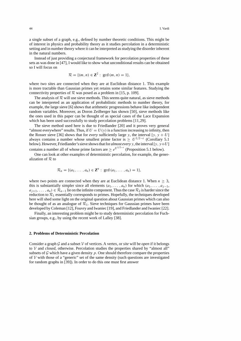
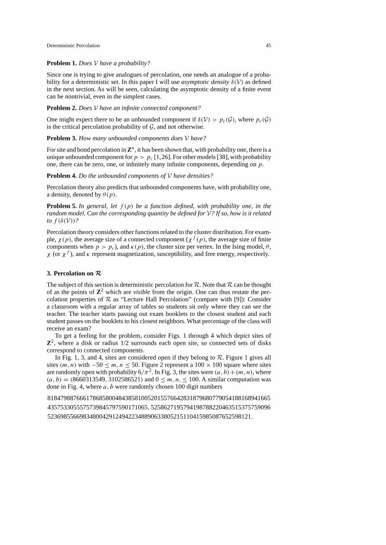
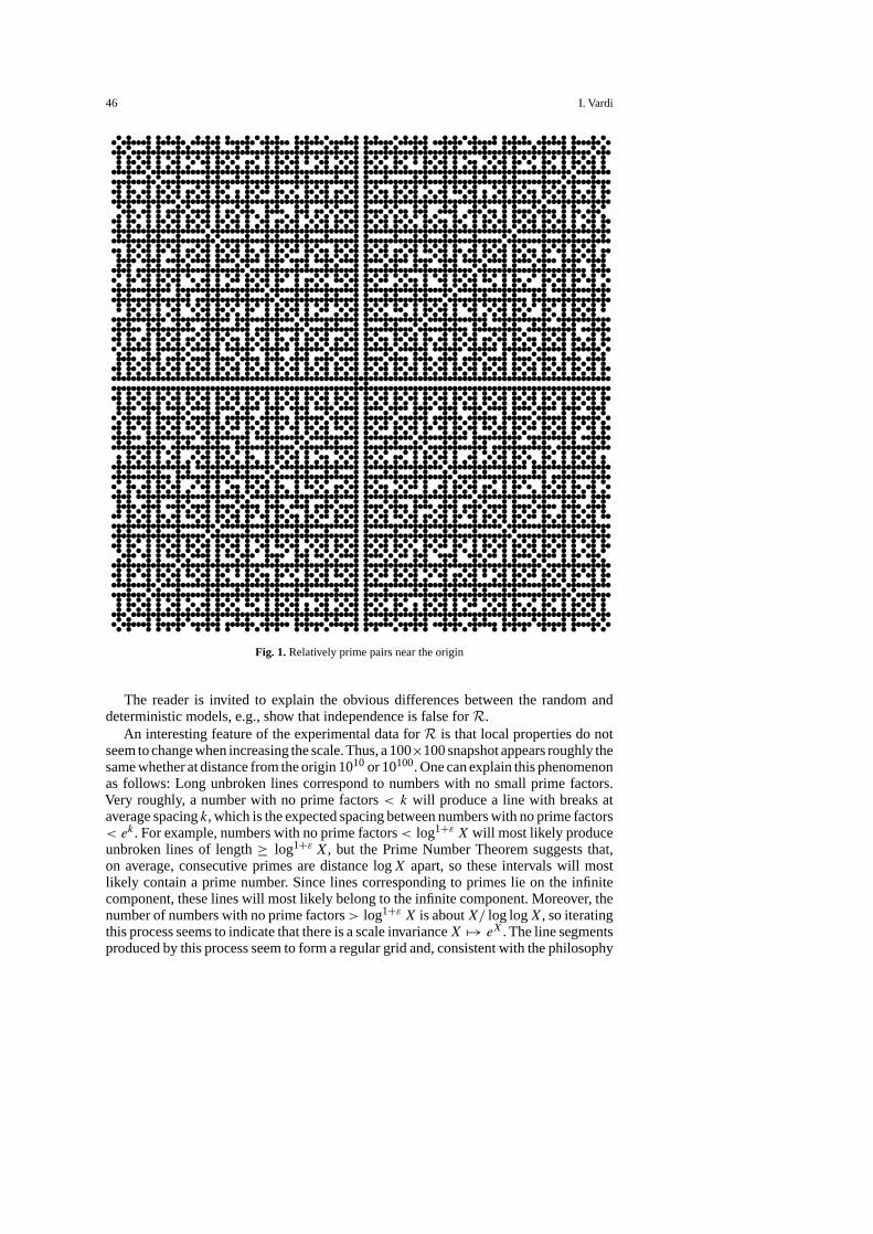
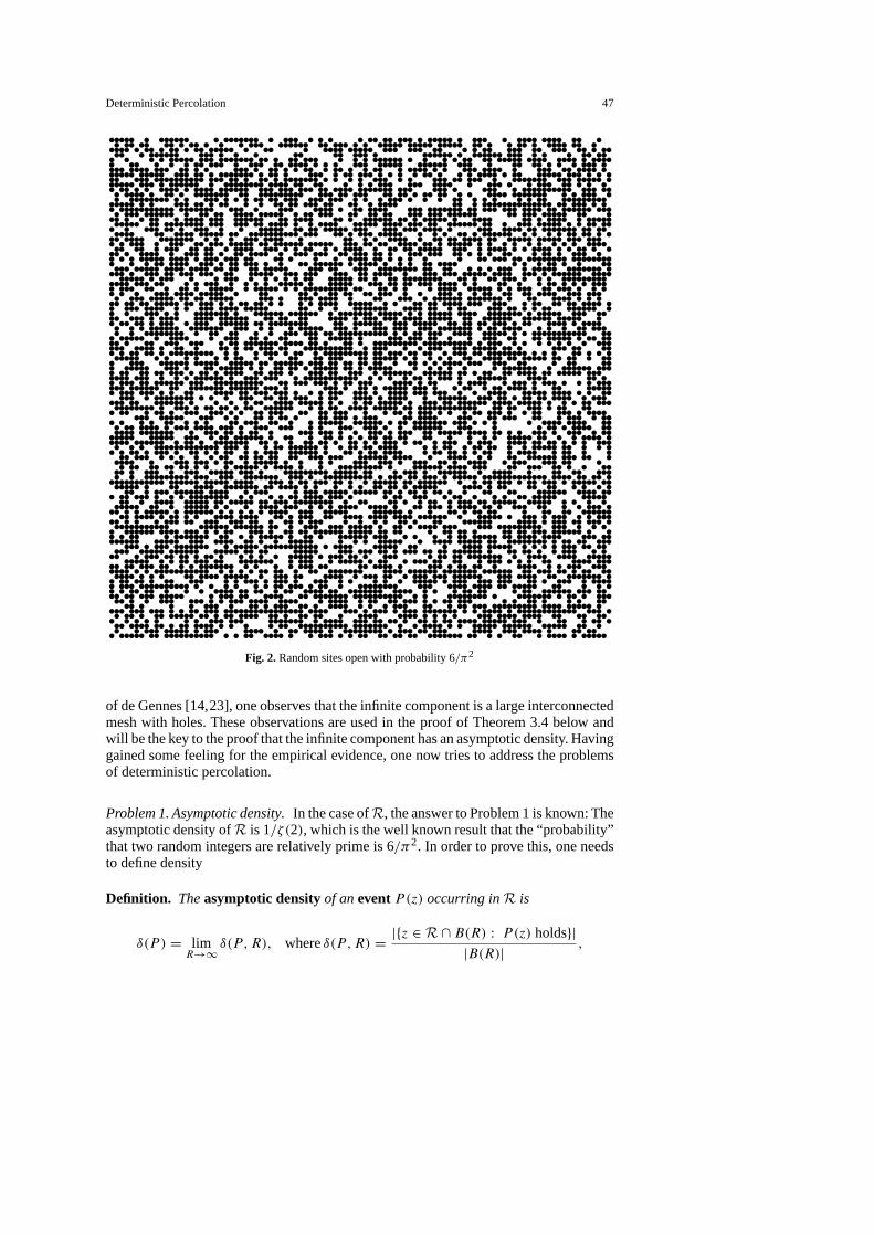
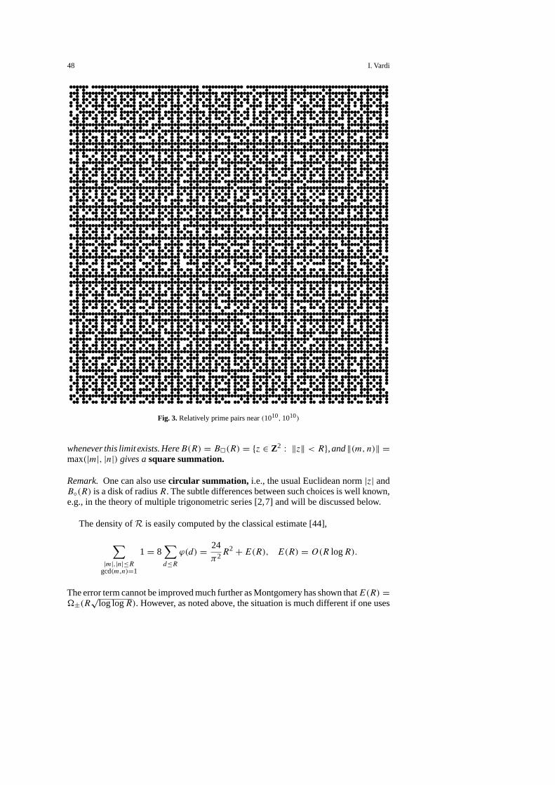
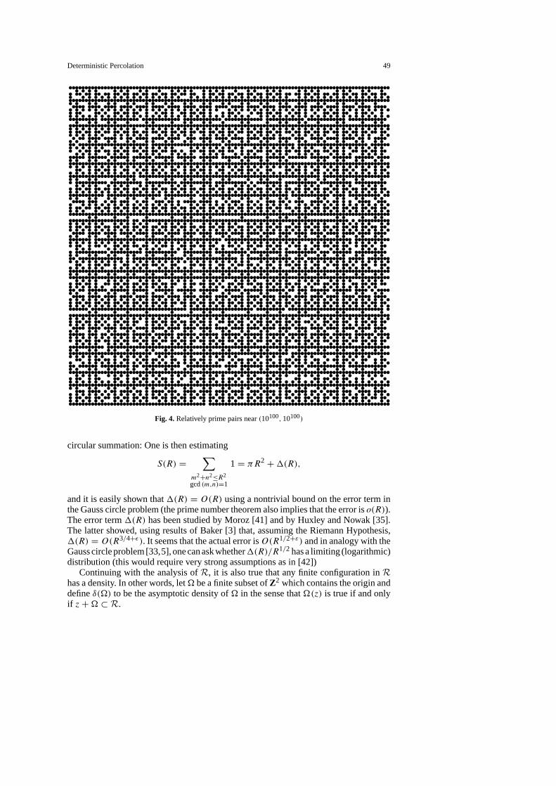
To get a feeling for the problem, consider Figs. 1 through 4 which depict sites ofZ2, where a disk or radius 1/2 surrounds each open site, so connected sets of diskscorrespond to connected components.

In Fig. 1, 3, and 4, sites are considered open if they belong toR. Figure 1 gives allsites(m, n) with −50 ≤ m, n ≤ 50. Figure 2 represent a 100× 100 square where sitesare randomly open with probability 6/π2. In Fig. 3, the sites were(a, b)+(m, n), where(a, b) = (8660313549,3102586521) and 0≤ m, n,≤ 100. A similar computation wasdone in Fig. 4, wherea, b were randomly chosen 100 digit numbers

818479887666178685800484385810052015576642831879680779054188168941665

4357533055575739845797590171065,5258627195794198788220463515375759096

523698556698348004291249422348890633805215110415985087652598121.

46 I. Vardi

Fig. 1.Relatively prime pairs near the origin

The reader is invited to explain the obvious differences between the random anddeterministic models, e.g., show that independence is false forR.

An interesting feature of the experimental data forR is that local properties do notseem to change when increasing the scale.Thus, a 100×100 snapshot appears roughly thesame whether at distance from the origin 1010 or 10100. One can explain this phenomenonas follows: Long unbroken lines correspond to numbers with no small prime factors.Very roughly, a number with no prime factors< k will produce a line with breaks ataverage spacingk, which is the expected spacing between numbers with no prime factors< ek. For example, numbers with no prime factors< log1+ε X will most likely produceunbroken lines of length≥ log1+ε X, but the Prime Number Theorem suggests that,on average, consecutive primes are distance logX apart, so these intervals will mostlikely contain a prime number. Since lines corresponding to primes lie on the infinitecomponent, these lines will most likely belong to the infinite component. Moreover, thenumber of numbers with no prime factors> log1+ε X is aboutX/ log logX, so iteratingthis process seems to indicate that there is a scale invarianceX 7→ eX. The line segmentsproduced by this process seem to form a regular grid and, consistent with the philosophy

Deterministic Percolation 47

Fig. 2.Random sites open with probability 6/π2

of de Gennes [14,23], one observes that the infinite component is a large interconnectedmesh with holes. These observations are used in the proof of Theorem 3.4 below andwill be the key to the proof that the infinite component has an asymptotic density. Havinggained some feeling for the empirical evidence, one now tries to address the problemsof deterministic percolation.

Problem 1. Asymptotic density.In the case ofR, the answer to Problem 1 is known: Theasymptotic density ofR is 1/ζ(2), which is the well known result that the “probability”that two random integers are relatively prime is 6/π2. In order to prove this, one needsto define density

Definition. Theasymptotic densityof aneventP(z) occurring inR is

δ(P ) = limR→∞ δ(P,R), whereδ(P,R) = |{z ∈ R ∩ B(R) : P(z) holds}|

|B(R)| ,

48 I. Vardi

Fig. 3.Relatively prime pairs near(1010,1010)

whenever this limit exists. HereB(R) = B2(R) = {z ∈ Z2 : ‖z‖ < R}, and‖(m, n)‖ =max(|m|, |n|) gives asquare summation.

Remark.One can also usecircular summation, i.e., the usual Euclidean norm|z| andB◦(R) is a disk of radiusR. The subtle differences between such choices is well known,e.g., in the theory of multiple trigonometric series [2,7] and will be discussed below.

The density ofR is easily computed by the classical estimate [44],

∑|m|,|n|≤R

gcd(m,n)=1

1 = 8∑d≤R

ϕ(d) = 24

π2R2 + E(R), E(R) = O(R logR).

The error term cannot be improved much further as Montgomery has shown thatE(R) =�±(R

√log logR). However, as noted above, the situation is much different if one uses

Deterministic Percolation 49

Fig. 4.Relatively prime pairs near(10100,10100)

circular summation: One is then estimating

S(R) =∑

m2+n2≤R2

gcd(m,n)=1

1 = πR2 +1(R),

and it is easily shown that1(R) = O(R) using a nontrivial bound on the error term inthe Gauss circle problem (the prime number theorem also implies that the error iso(R)).The error term1(R) has been studied by Moroz [41] and by Huxley and Nowak [35].The latter showed, using results of Baker [3] that, assuming the Riemann Hypothesis,1(R) = O(R3/4+ε). It seems that the actual error isO(R1/2+ε) and in analogy with theGauss circle problem [33,5], one can ask whether1(R)/R1/2 has a limiting (logarithmic)distribution (this would require very strong assumptions as in [42])

Continuing with the analysis ofR, it is also true that any finite configuration inRhas a density. In other words, let� be a finite subset ofZ2 which contains the origin anddefineδ(�) to be the asymptotic density of� in the sense that�(z) is true if and onlyif z+� ⊂ R.

50 I. Vardi

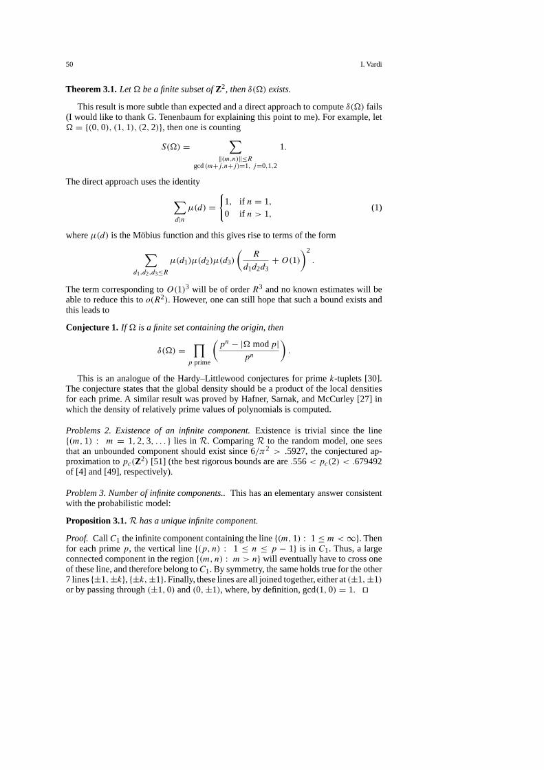
Theorem 3.1.Let� be a finite subset ofZ2, thenδ(�) exists.

This result is more subtle than expected and a direct approach to computeδ(�) fails(I would like to thank G. Tenenbaum for explaining this point to me). For example, let� = {(0,0), (1,1), (2,2)}, then one is counting

S(�) =∑

‖(m,n)‖≤Rgcd(m+j,n+j)=1, j=0,1,2

1.

The direct approach uses the identity

∑d|n

µ(d) ={

1, if n = 1,0 if n > 1,

(1)

whereµ(d) is the Möbius function and this gives rise to terms of the form

∑d1,d2,d3≤R

µ(d1)µ(d2)µ(d3)

(R

d1d2d3+O(1)

)2

.

The term corresponding toO(1)3 will be of orderR3 and no known estimates will beable to reduce this too(R2). However, one can still hope that such a bound exists andthis leads to

Conjecture 1. If � is a finite set containing the origin, then

δ(�) =∏

p prime

(pn − |� modp|

pn

).

This is an analogue of the Hardy–Littlewood conjectures for primek-tuplets [30].The conjecture states that the global density should be a product of the local densitiesfor each prime. A similar result was proved by Hafner, Sarnak, and McCurley [27] inwhich the density of relatively prime values of polynomials is computed.

Problems 2. Existence of an infinite component.Existence is trivial since the line{(m,1) : m = 1,2,3, . . . } lies in R. ComparingR to the random model, one seesthat an unbounded component should exist since 6/π2 > .5927, the conjectured ap-proximation topc(Z2) [51] (the best rigorous bounds are are.556< pc(2) < .679492of [4] and [49], respectively).

Problem 3. Number of infinite components..This has an elementary answer consistentwith the probabilistic model:

Proposition 3.1.R has a unique infinite component.

Proof. CallC1 the infinite component containing the line{(m,1) : 1 ≤ m < ∞}. Thenfor each primep, the vertical line{(p, n) : 1 ≤ n ≤ p − 1} is in C1. Thus, a largeconnected component in the region{(m, n) : m > n} will eventually have to cross oneof these line, and therefore belong toC1. By symmetry, the same holds true for the other7 lines{±1,±k}, {±k,±1}. Finally, these lines are all joined together, either at(±1,±1)or by passing through(±1,0) and(0,±1), where, by definition, gcd(1,0) = 1. ut

Deterministic Percolation 51

Problem 4. The asymptotic density of the infinite component.This is the main questionof this paper and I prove

Theorem 3.2.The infinite component ofR has an asymptotic density.

Let θ = θ(R) be the asymptotic density of the infinite component, i.e.,θ = δ(C∞),whereC∞(z) is true if and only ifz lies on the infinite component, which, by abuse ofnotation, will also be denoted byC∞. The value ofθ can examined experimentally andpreliminary computations seem to indicate thatθ/p(R2) ≈ .96± .01, i.e., about 96%of open sites lie on the unbounded component. In fact, I will prove

Theorem 3.3.The asymptotic density of the infinite component ofR is not zero.

Both these theorems are quite subtle and follow from

Theorem 3.4.Let f (R) be any function increasing to infinity then, except for a set ofzero asymptotic density, every(m, n) ∈ B(R) is surrounded by a rectangle of perimeter< f (R) all of whose edges are contained inC∞.

As noted above, this result is consistent with de Gennes’ philosophy that the infinitecomponent consists of a mesh with small holes [14,23]. Theorem 3.4 suggests that astronger result is true, namely if one defines rect(m, n) to be the perimeter of the smallestrectangle containing(m, n) all of whose edges are inC∞, then rect(m, n) should havea limiting distribution.

An examination of the proof of Theorem 3.2 (Sect. 8) reveals that it works withf (R)

in Theorem 3.4 replaced by(logR)1/2−ε, so Theorem 3.2 follows from the weakerresult of Lemma 7.3 below. It should be noted that one can similarly show that theinfinite component ofRn has an asymptotic density forn ≥ 3, and it is trivially nonzerosince it is≥ 6/π2 in these cases.

One can easily give an upper boundθ < 6/π2. Thus, considerγ (z) to be true ifz ≡ (4,15) (mod 30), thenz is isolated ifγ (z) andz ∈ R are both true. Since∑

‖(m,n)‖≤Rγ (z), (m,n)=1

=∑

gcd(d,30)=1d≤R

µ(d)∑

m≡4/d (mod 30)n≡15/d (mod 30)

‖(m,n)‖≤R/d

1 +O(R),

one gets

δ(γ ) = 1

302

∏p>5

(1 − 1

p2

)= 6

π2

∏p≤5

1

p2 − 1,

so

θ ≤ 6

π2 − 4δ(γ ) =(

1 − 1

144

)6

π2 = .993056

π2 .

More generally, define ananimalα to be a connected set containing the origin andα(z)

is true if z + ω ∈ R for everyω ∈ α, but z + ω 6∈ R if ω ∈ ∂α (a site is in∂α ifit is connected toα but not inα). It should be noted that this definition of animal isnot translation invariant, see [8] for general results on animals. The inclusion-exclusionprinciple implies that

δ(α) =∑s⊂∂α

(−1)nδ(α ∪ s),

52 I. Vardi

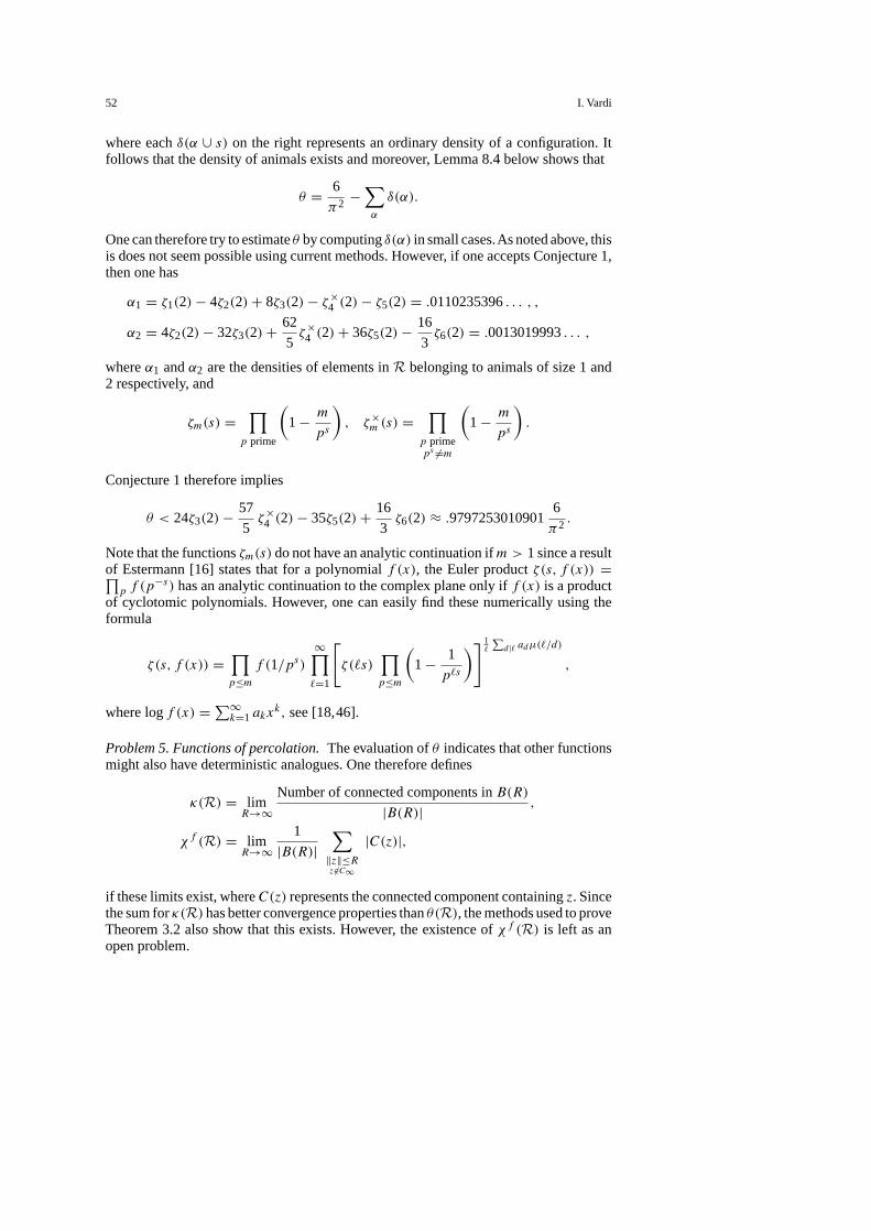
where eachδ(α ∪ s) on the right represents an ordinary density of a configuration. Itfollows that the density of animals exists and moreover, Lemma 8.4 below shows that

θ = 6

π2 −∑α

δ(α).

One can therefore try to estimateθ by computingδ(α) in small cases.As noted above, thisis does not seem possible using current methods. However, if one accepts Conjecture 1,then one has

α1 = ζ1(2)− 4ζ2(2)+ 8ζ3(2)− ζ×4 (2)− ζ5(2) = .0110235396. . . , ,

α2 = 4ζ2(2)− 32ζ3(2)+ 62

5ζ×

4 (2)+ 36ζ5(2)− 16

3ζ6(2) = .0013019993. . . ,

whereα1 andα2 are the densities of elements inR belonging to animals of size 1 and2 respectively, and

ζm(s) =∏

p prime

(1 − m

ps

), ζ×

m (s) =∏

p primeps 6=m

(1 − m

ps

).

Conjecture 1 therefore implies

θ < 24ζ3(2)− 57

5ζ×

4 (2)− 35ζ5(2)+ 16

3ζ6(2) ≈ .9797253010901

6

π2 .

Note that the functionsζm(s) do not have an analytic continuation ifm > 1 since a resultof Estermann [16] states that for a polynomialf (x), the Euler productζ(s, f (x)) =∏p f (p

−s) has an analytic continuation to the complex plane only iff (x) is a productof cyclotomic polynomials. However, one can easily find these numerically using theformula

ζ(s, f (x)) =∏p≤m

f (1/ps)∞∏`=1

[ζ(`s)

∏p≤m

(1 − 1

p`s

)] 1`

∑d|` adµ(`/d)

,

where logf (x) = ∑∞k=1 akx

k, see [18,46].

Problem 5. Functions of percolation.The evaluation ofθ indicates that other functionsmight also have deterministic analogues. One therefore defines

κ(R) = limR→∞

Number of connected components inB(R)

|B(R)| ,

χf (R) = limR→∞

1

|B(R)|∑

‖z‖≤Rz 6∈C∞

|C(z)|,

if these limits exist, whereC(z) represents the connected component containingz. Sincethe sum forκ(R)has better convergence properties thanθ(R), the methods used to proveTheorem 3.2 also show that this exists. However, the existence ofχf (R) is left as anopen problem.

Deterministic Percolation 53

A problem related to percolation is computing the asymptotics of the largestR-free square. This question is a generalization the Cramer conjecture [13] which statesthat the largest prime gap≤ R should tend to(logR)2 (though this is now believedto inaccurately model the primes [25]). One can compare results for the random anddeterministic models.

Proposition 3.2.LetFp(R) be the area of the largest closed square insideB(R), wheresites are open with probabilityp, then, with probability 1,

limR→∞

Fp(R)

logR= −2

log(1 − p).

Proposition 3.3.LetF(R) be the area of the largestR-free square inB(R), then

logR

(log logR)2� F(R)

logR� 1

log logR.

4. Finite Configurations have a Density

This section is devoted to the proof of Theorem 3.1. I will prove this by showing thatthe asymptotic density of a configuration is the limit of its density modulo a productof initial sets of primes. The idea is thatZ2 is approximated byZ2 mod

∏p≤X p and,

using an idea from ordinary percolation [26], one can think of some events as beingmonotonic.

Definition. Two integersm, n are relatively prime moduloh if gcd(m, n, h) = 1. Fur-thermore, let

δh(�,R) = |{(m, n) ∈ B(R) : �h(m, n)}|B(R)

,

where�h(m, n) means that�(m, n) holds as well as(m, n, h) = 1.

Lemma 4.1.δh(�) = limR→∞ δh(�,R) exists (and will be called the density of�moduloh).

Proof. This follows from the fact that this relative primality is periodic moduloh andthatB(h) tiles the plane. ut

The next step is to consider a product of an initial set of primesP(X) = ∏p≤X p and

let h = P(X). Thus the pairs relatively prime moduloP(X) will be an approximationto R. The main result thus follows from

Lemma 4.2.If Y > X andX → ∞, then δP (Y )(�, P (Y )) = δP (X)(�, P (X)) +O(|�|/X).Lemma 4.3.If bothX → ∞ andR/P (X) → ∞, then

δ(�,R) = δP (X)(�, P (X))+O(|�|/X + RP(X)/|B(R)|).

54 I. Vardi

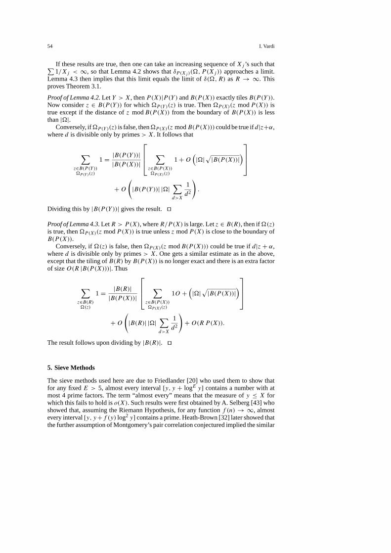
If these results are true, then one can take an increasing sequence ofXj ’s such that∑1/Xj < ∞, so that Lemma 4.2 shows thatδP (Xj )(�, P (Xj )) approaches a limit.

Lemma 4.3 then implies that this limit equals the limit ofδ(�,R) asR → ∞. Thisproves Theorem 3.1.

Proof of Lemma 4.2.LetY > X, thenP(X)|P(Y ) andB(P (X)) exactly tilesB(P (Y )).Now considerz ∈ B(P (Y )) for which�P(Y)(z) is true. Then�P(X)(z modP(X)) istrue except if the distance ofz modB(P (X)) from the boundary ofB(P (X)) is lessthan|�|.

Conversely, if�P(Y)(z) is false, then�P(X)(z modB(P (X))) could be true ifd|z+α,whered is divisible only by primes> X. It follows that

∑z∈B(P (Y ))�P(Y )(z)

1 = |B(P (Y ))||B(P (X))|

∑z∈B(P (X))�P(X)(z)

1 +O(|�|√|B(P (X))|

)

+O

(|B(P (Y ))| |�|

∑d>X

1

d2

).

Dividing this by|B(P (Y ))| gives the result.ut

Proof of Lemma 4.3.LetR > P(X), whereR/P (X) is large. Letz ∈ B(R), then if�(z)is true, then�P(X)(z modP(X)) is true unlessz modP(X) is close to the boundary ofB(P (X)).

Conversely, if�(z) is false, then�P(X)(z modB(P (X))) could be true ifd|z + α,whered is divisible only by primes> X. One gets a similar estimate as in the above,except that the tiling ofB(R) byB(P (X)) is no longer exact and there is an extra factorof sizeO(R |B(P (X)))|. Thus

∑z∈B(R)�(z)

1 = |B(R)||B(P (X))|

∑z∈B(P (X))�P(X)(z)

1O +(|�|√|B(P (X))|

)

+O

(|B(R)| |�|

∑d>X

1

d2

)+O(R P(X)).

The result follows upon dividing by|B(R)|. ut

5. Sieve Methods

The sieve methods used here are due to Friedlander [20] who used them to show thatfor any fixedE > 5, almost every interval[y, y + logE y] contains a number with atmost 4 prime factors. The term “almost every” means that the measure ofy ≤ X forwhich this fails to hold iso(X). Such results were first obtained by A. Selberg [43] whoshowed that, assuming the Riemann Hypothesis, for any functionf (n) → ∞, almostevery interval[y, y+f (y) log2 y] contains a prime. Heath-Brown [32] later showed thatthe further assumption of Montgomery’s pair correlation conjectured implied the similar

Deterministic Percolation 55

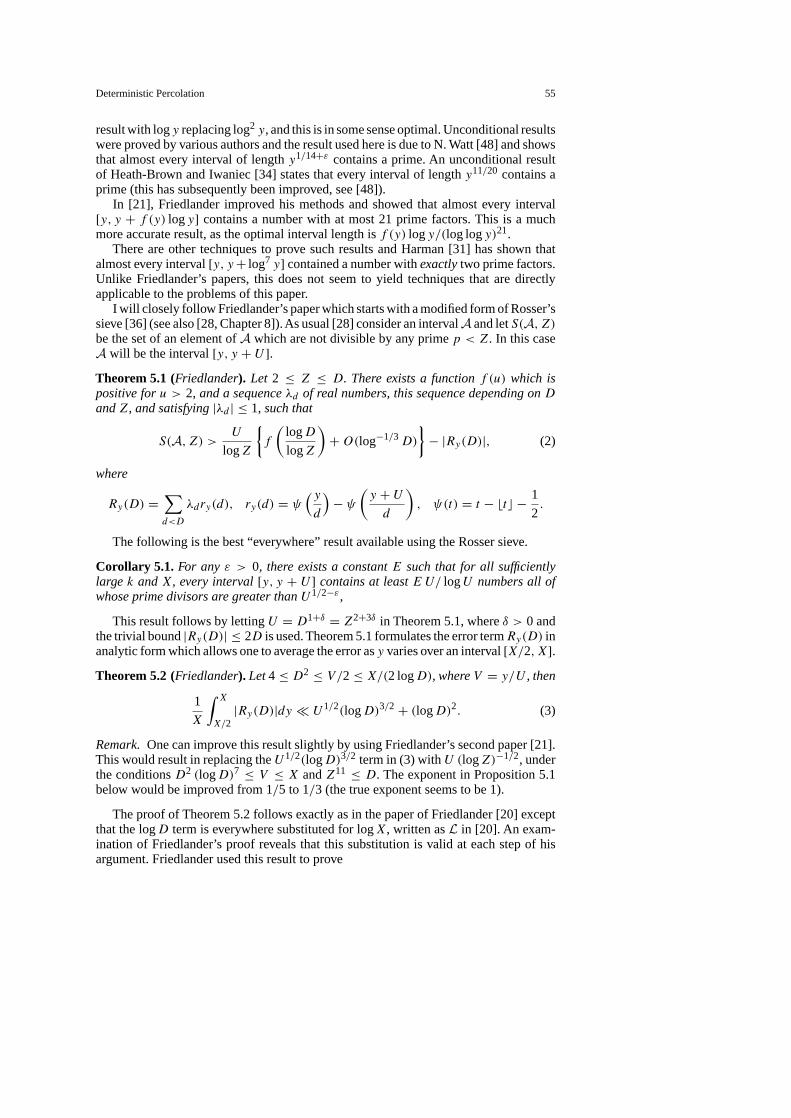
result with logy replacing log2 y, and this is in some sense optimal. Unconditional resultswere proved by various authors and the result used here is due to N. Watt [48] and showsthat almost every interval of lengthy1/14+ε contains a prime. An unconditional resultof Heath-Brown and Iwaniec [34] states that every interval of lengthy11/20 contains aprime (this has subsequently been improved, see [48]).

In [21], Friedlander improved his methods and showed that almost every interval[y, y + f (y) logy] contains a number with at most 21 prime factors. This is a muchmore accurate result, as the optimal interval length isf (y) logy/(log logy)21.

There are other techniques to prove such results and Harman [31] has shown thatalmost every interval[y, y+ log7 y] contained a number withexactlytwo prime factors.Unlike Friedlander’s papers, this does not seem to yield techniques that are directlyapplicable to the problems of this paper.

I will closely follow Friedlander’s paper which starts with a modified form of Rosser’ssieve [36] (see also [28, Chapter 8]).As usual [28] consider an intervalA and letS(A, Z)be the set of an element ofA which are not divisible by any primep < Z. In this caseA will be the interval[y, y + U ].Theorem 5.1 (Friedlander). Let 2 ≤ Z ≤ D. There exists a functionf (u) which ispositive foru > 2, and a sequenceλd of real numbers, this sequence depending onD

andZ, and satisfying|λd | ≤ 1, such that

S(A, Z) > U

logZ

{f

(logD

logZ

)+O(log−1/3D)

}− |Ry(D)|, (2)

where

Ry(D) =∑d<D

λdry(d), ry(d) = ψ(yd

)− ψ

(y + U

d

), ψ(t) = t − btc − 1

2.

The following is the best “everywhere” result available using the Rosser sieve.

Corollary 5.1. For any ε > 0, there exists a constantE such that for all sufficientlylarge k andX, every interval[y, y + U ] contains at leastE U/ logU numbers all ofwhose prime divisors are greater thanU1/2−ε,

This result follows by lettingU = D1+δ = Z2+3δ in Theorem 5.1, whereδ > 0 andthe trivial bound|Ry(D)| ≤ 2D is used. Theorem 5.1 formulates the error termRy(D) inanalytic form which allows one to average the error asy varies over an interval[X/2, X].Theorem 5.2 (Friedlander). Let4 ≤ D2 ≤ V/2 ≤ X/(2 logD), whereV = y/U , then

1

X

∫ X

X/2|Ry(D)|dy � U1/2(logD)3/2 + (logD)2. (3)

Remark.One can improve this result slightly by using Friedlander’s second paper [21].This would result in replacing theU1/2(logD)3/2 term in (3) withU (logZ)−1/2, underthe conditionsD2 (logD)7 ≤ V ≤ X andZ11 ≤ D. The exponent in Proposition 5.1below would be improved from 1/5 to 1/3 (the true exponent seems to be 1).

The proof of Theorem 5.2 follows exactly as in the paper of Friedlander [20] exceptthat the logD term is everywhere substituted for logX, written asL in [20]. An exam-ination of Friedlander’s proof reveals that this substitution is valid at each step of hisargument. Friedlander used this result to prove

56 I. Vardi

Theorem 5.3 (Friedlander). For anyA > 5, there is a constantc such that almostevery interval[y, y + (logy)A] contains at leastc (logy)A−1 numbersx such thatP−(x) > x1/4−ε, whereP−(x) is the smallest prime factor ofx (so x has at most 4prime factors).

This result will be generalized to arbitrary interval lengths of small size.

Proposition 5.1.Let g(R) be an unbounded increasing function such thatg(R) <

(logR)5. Given any fixedε > 0, then for all y < R, except for a set of measureO(R [g(R)]−ε/2), the interval[y, y + g(R)], contains anx with

P−(x) > exp([g(R)]1/5−ε).

Proof. One takes a largeT and has to show that almost ally ≤ T have anx ∈ [y, y +g(R)] with P−(x) > exp([g(R)]1/5−ε). Using the above notation, one writesU = g(R)

and in order to get the result of Proposition 5.1, one must chooseZ = eU1/5−ε

. Also, inorder to havef ((logD)/(logZ)) > 0, one takesD = Z2+ε.

SinceU → ∞, assume thaty > T/U and divide the interval[T/U, T ] into disjointsubintervals of the form(X, 2X]. TakingV = X/U and applying Theorem 5.1 gives alower bound

S(A, Z) > U4/5+ε {f (2 + ε′)+O((logD)−1/3)}

− |Ry(D)|,

so the main term has orderU4/5+ε. Now considerG ⊂ (X, 2X] given as the set ofy’sfor which |Ry(D)| > U4/5−ε. It follows that∫ 2X

X

|Ry(D)|dy > |G|U4/5−ε.

SinceU < (logX)5, one hasZ < e(logX)1−εand so

D2 ≤ e3(logX)1−ε ≤ X

2(logX)5≤ X

2U= V

2,

for all sufficiently largeX. Also, sinceD = exp((2 + ε)U1/5−ε), one hasU =C1(logX)5+ε′D for some constantsC1, ε

′, so

V

2= X

2U≤ C1

X

(logD)5≤ X

2 logD,

for all sufficiently largeX. The conditions of Theorem 5.2 are therefore satisfied, andapplying it gives∫ 2X

X

|Ry(D)|dy � X(U1/2(logD)3/2 + (logD)2) � XU4/5−3/2ε.

It follows that|G| � XU−ε/2 = o(R),

i.e., the proportion of exceptionaly’s goes to zero. Thus almost ally ∈ (X/2, X] have|Ry(D)| < U4/5−ε and this is dominated by the main termU4/5+ε of (3), soS(A, Z) isnonzero for almost all suchy. Taking the union of the intervals gives the result.ut

Deterministic Percolation 57

6. R-Free Squares

Before embarking on the rather daunting task of proving Theorem 3.4, I will do a“warmup” consisting of proving Propositions 3.2 and 3.3.

Proof of Proposition 3.2. (a) lim supFp(R)/ logR ≤ −2/ log(1 − p): Let c >

−2/ log(1−p), and at each site(m, n) inB(R), consider a square of areac log‖(m, n)‖and with lower left hand corner at(m, n). The probability that all sites in the square areclosed is(1 − p)c log‖(m,n)‖ < ‖(m, n)‖−2−ε, whereε > 0. Summing over all sites inZ2 gives ∑

(m,n)∈Z2

‖(m,n)‖>2

1

‖(m, n)‖2+ε ,

which converges. The Borel-Cantelli Lemma [17] shows that the probability of infinitelymany such squares being closed is zero.

(b) lim inf Fp(R)/ logR ≥ −2/ log(1 − p): Let c < −2/ log(1 − p) and for each site(m, n) with ‖(m, n)‖ > 2, consider a square of areac log‖(m, n)‖ with bottom lefthand corner atb(m, n) (log‖(m, n)‖)2c. As in part (a), it follows that each square has aprobability� ‖(m, n)‖−2−ε of being closed. Moreover, all these events are independentso the result follows from the Borel Cantelli Lemma and the divergence of

∑(m,n)∈Z2

‖(m,n)‖>2

(log‖(m, n)‖)2‖(m, n)‖2+ε . ut

Proof of Proposition 3.3.(a) Lower bound: Consider an integerk, and the firstk2 primesq1, . . . , qk2. By the Chinese Remainder Theorem, the following congruences have so-

lutionsm, n ≤ ∏k2

i=1 qi ,

m ≡ −imod

k∏j=1

qik+j

, n ≡ −j

mod

k∏j=1

qjk+i

,

so gcd(m+i, n+j) > 0, for 1≤ i, j ≤ k. The prime number theorem givesk2(1+ε′)k2>

‖(m, n)‖ > k2(1−ε)k, which yields the estimatek2 > (1 − ε′′) 12 logR/ log logR (one

can improve the 1/2 term toπ2/12).

(b) Upper bound:Assume that there is anR-free square{(m+i, n+j) : 1 ≤ i, j ≤ k}. ByCorollary 5.1, there arex1, . . . , x` ∈ [m+1, m+k] for whichP−(xi) > k1/2−ε, and suchthat` � k/ logk. Writexi = ∏ri

j=1 qeijij . One notes that ifq is a prime, then the number

of integers in a setS which are relatively prime toq is ≥ min{|S|(1 − 1/q), |S| − 1}.The asymptotic relation ∑

k1/2−ε<q≤kq prime

1

q∼ − log(1/2 − ε) < 1

thus implies that the number of integers in[m + 1, m + k] relatively prime toxi is� (1+ log(1/2− ε)) k− |{j ≤ ri : qij ≥ k}|, and so eachri > (1+ log(1/2− 2ε)) k.

58 I. Vardi

One further notes that gcd(xi, xj ) ≤ k for i 6= j , so thatxi andxj can share at most 2distinct prime factors. This implies that the number of distinctqij ’s is � k2/ logk. Theprime number theorem gives

∏i=1

xi �∏

y<q≤D k2

q prime

q = eD k2−k1/2−ε+o(1),

for some constantD, and so logxi � k logk for all i. This therefore gives logR �k logk and the result follows since logk is of order log logR. ut

7. The Structure of the Infinite Component

In this section, I prove Theorem 3.4. One begins identifying some subsets of the infinitecomponent.

Lemma 7.1.The following sets are inC∞:

(1) {(m,1) : m > 0}. (2) {(p, n) : p > n}, p prime.

(3) {(m, q) : q < m < (q/2)20/11, q 6 |m}, qprime.

Proof. The first two results were proved above. The third follows from the unconditionalresult of Heath-Brown and Iwaniec [34] which states that every interval of lengthy11/20

contains a prime (this has subsequently been improved, see [48]). Thus, ifq 6 |m, thensinceq > 2m11/20, one of the intervals[m+m11/20] or [m−m11/20, m] has none of itselements divisible byq and the corresponding line segment lies completely inR. By theresult of Heath-Brown and Iwaniec, this line segment will cross a line{(p, n)}, wherep is prime, and by (2), this is inC∞, so(m, q) is also inC∞. ut

One proceeds by proving an initial version of Theorem 3.4.

Lemma 7.2.All but O(R2/ logR) pairs of B(R) are surrounded by a rectangle ofperimeterO((logR)7) all of whose edges are contained inC∞.

Proof. Consider the set

S0 = {(m, n) ∈ B(R) : ∃ n′, P−(n′) > R1/5, (logR)7 + n > n′ > n,minimal,

(d, n′) = 1 if |d −m| < R1/13, ∃p ∈ [m− R1/13, m+ R1/13]}.By Watt’s result that almost every interval of lengthy1/14+ε contains a prime,

E0,1 = {(m, n) ∈ B(R) : [m− R1/13, m+ R1/13] has no primes}has density zero. In fact, his result shows that|E0,1| � R2/(logR)2, since substitut-ing E = 3 in Theorem 1 of [48] already gives this estimate for intervals of lengthR1/14(logR)22.

Next, if

E0,2 = {(m, n) ∈ B(R) : P−(n′) ≤ R1/5, for all (logR)7 + n > n′ > n},

Deterministic Percolation 59

then |E1,2| � R2/ logR. This bound follows by an argument similar to the proof ofProposition 5.1: Partition[R1/2, R] into intervals of the form[X,2X] and in each ofthese intervals, letU = (logX)7, D = V 1/2/2, and for a fixed 1/10 > ε > 0, letZ = D1/2−ε. The main term in Eq. (2) of Theorem 5.1 is then� (logX)6 whileTheorem 5.2 gives

1

X

∫ 2X

X

|Ry(D)|dy � (logX)5.

ThereforeG defined as the set ofy ∈ (X, 2X] for which |Ry(D)| � (logX)6 satisfies|G| � X/ logX.

Finally, one considers

E0,3 = {(m, n) ∈ B(R) : P−(n′) > R1/5, (logR)7 + n > n′ > n, minimal,

∃d |d −m| < R1/13, (d, n′) > 1}.But if P−(n′) > R1/5, then

|E0,3| � R(logR)7∑

P−(n′)>R1/5

|d−m|<R1/13, (d,n′)>1

1 � R1+1/13(logR)7R∑p|n′

R

p

� R2+1/13−1/5 (logR)7 � R2

logR.

SinceB(R)− S0 ⊂ E0,1 ∪ E0,2 ∪ E0,3, it follows that|B(R)− S0| � R2/ logR, andsoS0 represents almost all points ofB(R).

An examination of the definition ofS0 shows that for every(m, n) ∈ S0 there isan unbroken horizontal line segmentL0,1(m, n) ⊂ C∞ of lengthR1/13, centered at(m, n) and which passes above(m, n) within distanceO((logR)7), and which crossesa vertical line{(p, n)}, wherep is prime. By Lemma 7.1 (2), this vertical line is inC∞,so it follows thatL0,1(m, n) is also inC∞.

Replacing the conditionn′ > n with n′ < n yields the similar result with a linesegmentL0,2(m, n), passing below(m, n). To construct the corresponding vertical linesegmentsL0,3(m, n),L0,4(m, n), one must include the condition thatm, n � R11/20 inorder to apply part 3 of Lemma 7.1. The result then follows.ut

The next iteration already contains most of the ideas of the general procedure and isincluded in order to give a self-contained proof of Theorem 3.3.

Lemma 7.3.All butO(R2/(log logR)3) pairs ofB(R) are surrounded by a rectangleof perimeterO((log logR)36) all of whose edges are contained inC∞.

Proof. Consider the set

S1 = {(m, n) ∈ B(R) : ∃m′ P−(m′) > (logR)42,

(log logR)36 +m > m′ > m, minimal,

(m′, d) = 1, |d − n| < (logR)40.}.Now let

E1,1 = {(m, n) ∈ B(R) : P−(m′) < (logR)42, for all (log logR)36 +m > m′ > m}.

60 I. Vardi

By Proposition 5.1, for almost ally, [y, y + (log logR)36] contains an integerx withP−(x) > exp((log logR)36(1/5−ε)), and this is> (logR)42 for all sufficiently largeR.The error term of Proposition 5.1 gives

|E1,1| � R2

(log logR)36ε/2 = R2

(log logR)3,

by lettingε = 1/6. Next, one considers

E1,2 = {(m, n) ∈ B(R) : P−(m′) > (logR)42,

(log logR)36 +m > m′ > m, minimal,

∃d |d − n| < (logR)40, (m′, d) > 1}.As before, one gets

|E1,2| � R(log logR)36∑

P−(m′)>(logR)42

|d−n|<(logR)40, (m′,d)>1

1

� R (log logR)36(logR)40∑p|m′

R

p� R2 (log logR)37

(logR)2

� R2

logR,

for all sufficiently largeR. This last estimate used the fact that ifP−(m′) > (logR)42

andm′ < R, thenm′ can have at mostO(logR/ log logR) prime factors.It follows thatS1 consists of almost all elements ofB(R). The definition ofS1 then

shows that for almost all(m, n) ∈ B(R), there is a line segmentL1,1(m, n) ⊂ R oflength at least(logR)40, centered at(m, n) and which passes by(m, n) at distanceO((log logR)36).

One now observes thatS0 ∩ S1 also comprises almost all elements ofB(R). Thedefinition ofS0 implies that for almost all(m, n), the line segmentL1,1(m, n) intersectsa rectangle of perimeterO((logR)7) whose edges lie inC∞ (note that these extendin C∞ to lengthR1/13), soL1,1(m, n) will also be contained inC∞. Clearly, one cansimilarly show that for almost all(m, n), there are line segmentsL1,j ⊂ R, j = 2,3,4,of length(logR)40 and which pass within(log logR)36 of (m, n) on all four sides, andby the same argumentL1,j ⊂ C∞, j = 2,3,4. ut

An examination of the proof of Lemma 7.3 reveals that the obstacle in continuingthis process is the term

∑p|m′ 1/p, which must beo(1). The trivial estimate

∑p|m

1

p� ω(m)

P−(m)(4)

was used and this will only allow one more iteration, if one first removes allm for whichω(n) > 2 log logR (as is well known, this set has zero density [44]). In fact, in thiscontext, it is easy to improve substantially on (4), as was noted to me by G. Tenenbaum.

Deterministic Percolation 61

Lemma 7.4.Letf (R) be any function increasing to infinity, then except for a set ofm

of sizeO(R/√f (R) logf (R)), one has the bound

∑p|m

p≥f (R)

1

p� 1√

f (R) logf (R).

Proof. One uses the simple estimate

∑m≤R

∑p|m

p≥f (R)

1

p=

∑p≥f (R)

R

p2 = R

f (R) logf (R).

This result reflects the fact that∑p|m 1/p has a limiting density, as follows easily from

the Erdos–Wintner Theorem [44].utThis result allows one to iterate the above argument. Recall that rect(m, n) is the

perimeter of the smallest rectangle surrounding(m, n) which has all its edges inC∞.

Lemma 7.5.Let log1 z = logz andlogk+1 z = log(logk z), and letexpk z be the inverseof logk z, then forR > expk+2(1015),

|(m, n) ∈ B(R) : rect(m, n) ≤ (logk+1R)36}| = |B(R)|

[1 −O

(1

(logk+1R)3

)],

(5)

where theO( ) term is independent ofk.

Proof. One proves this by induction onk. The initial stepk = 1 is exactly Lemma 7.3.Now assume that (5) holds fork, then I will show that it holds fork + 1.

Thus assume that one has constructed for almost all(m, n), line segmentsLk,j (m, n),j = 1,2,3,4, as above, but of length(logk R)

40, which pass within(logk+1R)36, are

centered at(m, n) and lie completely inC∞. In particular, one assumes that the set

Sk = {(m, n) ∈ B(R) : ∃n′ P−(n′) > (logk R)100,

(logk+1R)36 + n > n′ > n, minimal,

(d, n′) = 1, |d −m| < (logk R)40, (m, n′) ∈ C∞},

is such that|B(R)− Sk| � R2/(logk+1R)3. One then considers

Sk+1 = {(m, n) ∈ B(R) : ∃m′ P−(m′) > (logk+1R)100,

(logk+2R)36 +m > m′ > m, minimal,

(m′, d) = 1, |d − n| < (logk+1R)40}.

Now let

Ek+1,1 = {(m, n) ∈ B(R) : P−(m′) < (logk+1R)100,

for all (logk+2R)36 +m > m′ > m}.

62 I. Vardi

By Proposition 5.1, for anyε > 0, except forO(R/(logk+2R)36ε/2)values ofy, the inter-

val [y, y+ (logk+2R)36] contains an integerx with P−(x) > exp((logk+2R)

36(1/5−ε)).Letting ε = 1/6, this says that except forO(R/(logk+2R)

3) values ofy, the interval[y, y + (logk+2R)

36] contains an integerx with P−(x) > exp((logk+2R)1+2/15). This

last quantity is eventually> (logk+1R)100, in particular, when logk+2R > 10015/2, i.e.,

whenR > expk+2(1015). Thus, one concludes that

|Ek+1,1| � R2

(logk+2R)3 , for R > expk+2(1015).

Next, one considers

Ek+1,2 = {(m, n) ∈ B(R) : P−(m′) > (logk+1R)100,

(logk+2R)36 +m > m′ > m, minimal,

∃d, |d − n| < (logk+1R)40, (m′, d) > 1}.

As before, one gets

|Ek+1,2| � R(logk+2R)36

∑P−(m′)>(logk+1R)

100

|d−n|<(logk+1R)40, (m′,d)>1

1

� R (logk+2R)36(logk+1R)

40∑m≤R

P−(m)>(logk+1R)100

∑p|m

1

p.

Now let

Ek+1,3 = {(m, n) ∈ B(R) :∑p|m′

p>(logk+1R)100

1

p≥ 1

(logk+1R)50√

logk+2R

for all (logk+2R)36 +m > m′ > m}.

Applying Lemma 7.4 gives

|Ek+1,3| � R2 (logk+2R)36

(logk+1R)50√

logk+2R,

so

|Ek+1,2 − Ek+1,3| � R2(logk+2R)36(logk+1R)

40

(logk+1R)50√

logk+1R� R2

logk+1R,

whenever(logk+1R)9 > (logk+2R)

36, for example, whenR > expk+2(16). It followsthat Sk+1 consists of almost all elements ofB(R), where the exceptional set is�R2/(logk+2R)

3.The definition ofSk+1 also shows that for almost all(m, n) ∈ B(R), there is a line

segmentLk+1,1(m, n) ⊂ R of length at least(logk+1R)40, centered at(m, n) and which

passes by(m, n) at distanceO((logk+2R)36).

Deterministic Percolation 63

One now observes thatSk ∩ Sk+1 also comprises almost all elements ofB(R) exceptfor an exceptional set of size

� R2

(logk+1R)3 + R2

(logk+2R)3 = (1 + Ak)

R2

(logk+1R)3 ,

for sufficiently largeR, where

k∏j=1

(1 + Aj) �k∏j=1

[1 +O

(1

(logj R)3

)]= O(1).

The definition ofSk+1 implies that for almost all(m, n), the line segmentLk+1,1(m, n)

of length (logk+1R)40 will intersect the perimeter of the rectangle of perimeter

(logk+1R)36 constructed in the previous iteration (note that its sides extend to line

segments inC∞ of length (logk R)40). Since the sides of this rectangle lie inC∞, it

follows thatLk+1,1(m, n)will also be contained inC∞. Thus, the line segments definedin Sk+1 also lie inC∞.

Clearly, one can similarly show that for almost all(m, n), there are line segmentsLk+1,j ⊂ R, j = 2,3,4, of length(logk+1R)

40 and which pass within(logk+2R)36 of

(m, n) on all four sides, andLk+1,j ⊂ C∞, j = 2,3,4. utProof of Theorem 3.4.Assume that there is a functionf (R) increasing to infinity, and afixedλ > 0 such that for at leastλR2

i pairs(m, n) one has rect(m, n) > f (Ri), whereRi is a sequence increasing to infinity.

One defines log∗ z to be the minimum number of iterations of log required to be≤ 2,i.e., loglog∗ z z ≤ 2. Let k = log∗ R − log∗ f (R) − 2, then logk R � logf (R) for allsufficiently largeR.

One can now apply Lemma 7.5 since the bound

expk+2(1015) = explog∗ R−logf (R)+4(1015) � logR = o(R)

holds. Furthermore, one has

1

(logk+1R)3 � 1

log4 f (R)→ 0,

since logk R � log3 f (R)andf (R) → ∞. Substituting this in (5) shows that for almostall (m, n) ∈ B(R) one has rect(m, n) ≤ f (R), which contradicts the above assumption.The result follows. ut

Proof of Theorem 3.3.Assuming Theorem 3.2, then this follows directly from Theo-rem 3.4. For if the result were not true, then there would be a functionf (R) increasing toinfinity such thatθ(R) < 1/f (R) for all sufficiently largeR. However, Theorem 3.4 im-plies that for sufficiently largeR, almost all points ofB(R) are surrounded by a rectangleof perimeter

√f (R) all of whose edges lie inC∞. This implies thatθ(R) � 1/

√f (R)

which is a contradiction.ut

64 I. Vardi

8. The Infinite Ccomponent has a Density

As in Sect. 4, the idea is to compare the density of the infinite component in a big square

θ(R) = |B(R) ∩ C∞||B(R)|

with this density modulo a product of primes. Thus, let

θh = limR→∞

|{(m, n) ∈ B(R) : (m, n) ∈ infinite component moduloh}||B(R)| .

The following gives a local characterization of the infinite component moduloh.

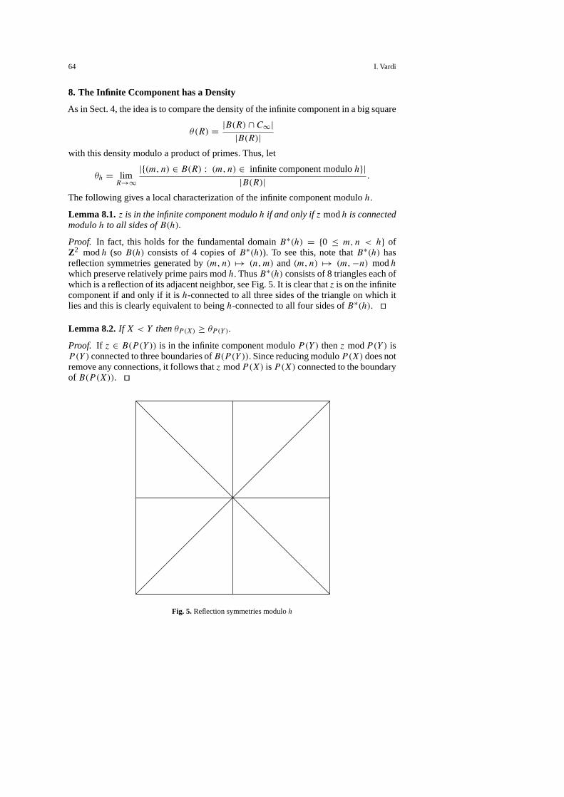
Lemma 8.1.z is in the infinite component moduloh if and only ifz modh is connectedmoduloh to all sides ofB(h).

Proof. In fact, this holds for the fundamental domainB∗(h) = {0 ≤ m, n < h} ofZ2 modh (soB(h) consists of 4 copies ofB∗(h)). To see this, note thatB∗(h) hasreflection symmetries generated by(m, n) 7→ (n,m) and(m, n) 7→ (m,−n) modhwhich preserve relatively prime pairs modh. ThusB∗(h) consists of 8 triangles each ofwhich is a reflection of its adjacent neighbor, see Fig. 5. It is clear thatz is on the infinitecomponent if and only if it ish-connected to all three sides of the triangle on which itlies and this is clearly equivalent to beingh-connected to all four sides ofB∗(h). ut

Lemma 8.2.If X < Y thenθP (X) ≥ θP (Y ).

Proof. If z ∈ B(P (Y )) is in the infinite component moduloP(Y ) thenz modP(Y ) isP(Y ) connected to three boundaries ofB(P (Y )). Since reducing moduloP(X) does notremove any connections, it follows thatz modP(X) isP(X) connected to the boundaryof B(P (X)). ut

Fig. 5.Reflection symmetries moduloh

Deterministic Percolation 65

One concludes thatθP (X) is decreasing and therefore the limitθ∗ = limX→∞ θP (X)exists.

Lemma 8.3.If bothX → ∞ andR/P (X) → ∞, thenθ(R) ≤ θP (X) + o(1).

Proof. This follows exactly as in the above also following the proof of Lemma 4.3.Note that the boundary error in tilingB(R) with B(P (X)) is O(P (X)/R) = o(1) byassumption. ut

One therefore hasθ(R) ≤ θ∗ + o(1) and the main result follows from

Lemma 8.4. limR→∞ θ(R) = θ∗.

Proof. If θ∗ = 0, then Lemma 8.3 shows thatθ = 0 as well and there is nothing toprove. On the other hand, ifθ∗ > 0 consider a largeR and by Lemma 8.2, find alargeX such thatθP (X) is very close toθ∗, with P(X) < R andR/P (X) large. Sincethe prime number theorem says thatP(X) = eX+o(1), one can chooseX such thatR1/2/4< P(X) < R1/2. It follows thatX is of order logR, i.e., there are two constantsA,B, such thatA logR < X < B logR.

Now going fromR moduloP(X) toR inB(R) removes at most|B(R)| ∑d>X 1/d2

� |B(R)|/X elements. So, by the above estimate, one is removingO(R2/ logR) sites.By Lemma 7.3, given 0< ε < 1/2, one can surround almost all sites with aC∞ rectan-gle of perimeter< (logR)1/2−ε. Thus apart from a set of zero density, each individualremoval can disconnect at most(logR)1−2ε sites from the connected component (notethat none of the elements on the rectangles specified by Lemma 7.3 are removed, sincethese belong toC∞ of R). It follows that at mostO(R2(logR)1−2ε/ logR) sites are dis-connected, a vanishingly small percentage of the infinite connected component moduloP(X). This implies thatθ(R) is asymptotically close toθP (X). ut

Acknowledgement.I would like to thank Cécile Dartyge for checking the method of Sect. 7 and GéraldTenenbaum for helpful comments and a crucial observation (Lemma 7.4).

References

1. Aizenman, M., Kesten, H., Newman, C.M.: Uniqueness of the infinite cluster and continuity of connec-tivity functions for short and long range percolation. Commun. Math. Phys.111, 505–531 (1987)

2. Ash, J.M., Wang, G.: A survey of uniqueness questions in multiple trigonometric series. In: Harper, L.H.(editor),Harmonic Analysis and nonlinear differential equationsAmerican Math. Soc. Contemp. Math.208, 1997, pp. 35–71

3. Baker, R.C.: The square–free divisor problem. Quart. J. Math. Oxford45, 269–277 (1994)4. van den Berg, J., Ermakov, A.: A new lower bound for the critical probability of site percolation on the

square lattice. Random Structures and Algorithms8, (1996), 199–2125. Bleher, P.M., Cheng, Z., Dyson, F.J., Lebowitz, J.L.: Distribution of the error term for the number of

lattice points inside a shifted circle. Commun. Math. Phys.54, 433–469 (1993)6. Bombieri, E.:Le grand crible dans la théorie analytique des nombres. 2nd edition, Astérisque18, 19877. Bourgain, J.: Spherical summation and uniqueness of multiple trigonometric series. Int. Math. Research

Notices3, 93–107 (1996)8. Bousquet-Mélou, M.: Percolation models and animals. European J. Combin.17, 343–369 (1996)9. Bousquet-Mélou, M., Eriksson, K.: Lecture hall partitions. Ramanujan J.1, 101–111 (1997)

10. Broadbent, S.R., Hammersley, J.M.: Percolation processes. Proc. Cambridge Phil. Soc.53, 629–641(1957)

11. Brydges, D.C., Spencer, T.: Self–avoiding walk in 5 or more dimensions. Commun. Math. Phys.97,125–148 (1985)

12. Coleman, M.D.: The Rosser–Iwaniec sieve in number fields, with an application. Acta Arithmetica66,53–83 (1993)

66 I. Vardi

13. Cramér, H.: On the order of magnitude of the difference between consecutive prime numbers. ActaArithmetica2, 23–46 (1937)

14. Efros, A.L.:Physics and Geometry of Disorder, Percolation Theory. Moscow: Mir, 198615. Erdos, P., Gruber, P.M., Hammer, J.:Lattice Points. New York: Longman, Wiley, 198916. Estermann, T.: On certain functions represented by Dirichlet series. Proc. London Math. Soc.27, 435–448

(1928)17. Feller, W.:An Introduction to Probability Theory and its Applications. Vol. I , New York: Wiley, 196418. Flajolet, P., Vardi, I.: Zeta expansions of classical constants. Preprint (1996)19. Fouvry, E., Iwaniec, H.: Gaussian primes. Acta Arithmetica79, 249–287 (1997)20. Friedlander, J.B.: Sifting short intervals. Math. Proc. Camb. Phil. Soc.91, 9–15 (1982)21. Friedlander, J.B.: Sifting short intervals II. Math. Proc. Camb. Phil. Soc.92, 381–384 (1982)22. Friedlander, J.B., Iwaniec, H.: Using a parity-sensitive sieve to count prime values of a polynomial. Proc.

Nat. Acad. Sci. U.S.A.94, 1054–1058 (1997)23. de Gennes, P.G.: La percolation: Un concept unificateur. La Recherche7, 919–927 (1976)24. Gethner, E., Wagon, S., Wick, B.: A stroll through the Gaussian primes. American Math. Monthly105,

327–337 (1998)25. Granville, A.: Unexpected irregularities in the distribution of prime numbers. Proceedings of the Interna-

tional Congress of Mathematicians, (Zurich, 1994). Basel: Birkhäuser, 1995, pp. 388–39926. Grimmett, G.:Percolation. New York: Springer-Verlag, 198927. Hafner, J.L., Sarnak, P., McCurley, K.: Relatively prime values of polynomials. In: Knopp, M., Sheingorn,

M. (eds),A tribute to Emil Grosswald: Number theory and related analysis. Contemp. Math.143, Amer.Math. Soc., Providence, RI: 1993, pp.437–443

28. Halberstam, H.,Richert, H.–E.:Sieve Methods. New York: Academic Press, 197429. Hara, T., Slade, G.: Mean-field critical behavior for percolation in high dimensions. Commun. Math.

Phys.128, 339–391 (1990)30. Hardy, G.H., Littlewood, J.E.: Some problems of ‘Partitio Numerorum’III: On the expression of a number

as a sum of primes. Acta Math.44, 1–70, also In: G.H. Hardy:Coll. Papers,vol. 1, 1922, pp.561–63031. Harman, G.: Almost primes in short intervals. Math. Ann.258, 107–112 (1981)32. Heath-Brown, D.R.: Gaps between primes and the pair correlation of zeros of the zeta–function. Acta

Arithmetica41, 85–99 (1982)33. Heath-Brown, D.R.: The distribution and moments of the error term in the Dirichlet divisor problems.

Acta Arithmetica60, 389–415 (1992)34. Heath-Brown, D.R., Iwaniec, H.: On the difference between consecutive primes. Invent. Math.55, 49–69

(1979)35. Huxley, M.N., Nowak, W.G.: Primitive lattice points in convex planar domains. Acta Arithmetica76,

271–283 (1996)36. Iwaniec, H.: Rosser’s sieve. Acta Arithmetica36, 171–202 (1980)37. Iwaniec, I., Mozzochi, C.J.: On the divisor and circle problems. J. Number Theory29, 60–93 (1988)38. Lalley, S.: Percolation on Fuchsian groups. Ann. Inst. H. Poincaré Probab. Statist.34, 151–177 (1998)39. Lubotzky, A., Phillips, R., Sarnak, P.: Ramanujan graphs. Combinatorica8, 261–277 (1988)40. Montgomery, H.L.: Fluctuations in the mean of Euler’s phi function. Proc. Indian Acad. Sci. Math. Sci.

97, 239–245 (1987)41. Moroz, B.Z.: On the number of primitive lattice points in plane domains. Monatschrift Math.99, 37–43

(1985)42. Sarnak, P., Rubinstein, M.: Chebyshev’s bias. Experimental Math.3, 173–197 (1994)43. Selberg, A.: On the normal density of primes in short intervals, and the difference between consecutive

primes. Arch. Math. Naturvid.47, 87–105 (1943)44. Tenenbaum, G.:Introduction to analytic and probabilistic number theory. Cambridge: Cambridge Uni-

versity Press, 199545. Turán, P.: On a theorem of Hardy and Ramanujan. J. London Math. Soc.9, 274–276 (1934)46. Vardi, I.:Computational Recreations in Mathematica. Reading, MA: Addison–Wesley, 199147. Vardi, I.: Prime Percolation. Experimental Mathematics7, 275–289 (1998)48. Watt, N.: Short intervals almost all containing primes. Acta Arithmetica72, 131–167 (1995)49. Wierman, J.C.: Substitution method critical probability bounds for the square lattice site percolation

model. Combin. Probab. Comput.4, 181–188 (1995)50. Zeilberger, D.: The Abstract Lace Expansion. Adv. Appl. Math.19, 355–359 (1997)51. Ziff, R.M., Sapoval, B.: The efficient determination of the percolation threshold by a frontier–generating

walk in a gradient. J. Phys A: Math. Gen.19, L1169–L1172 (1986)

Communicated by P. Sarnak