Deterministic Global Optimization for Dynamic SystemsUsing Interval Analysis

Youdong Lin and Mark A. Stadtherr

Department of Chemical and Biomolecular Engineering

University of Notre Dame, Notre Dame, IN, USA

12th GAMM–IMACS International Symposium on Scientific Computing, Computer Arithmetic and Validated NumericsDuisburg, Germany, 26–29 September 2006

Outline

• Background

• Tools

– Interval Analysis

– Taylor Models

– Validated Solutions of Parametric ODE Systems

• Algorithm Summary

• Computational Studies

• Concluding Remarks

2

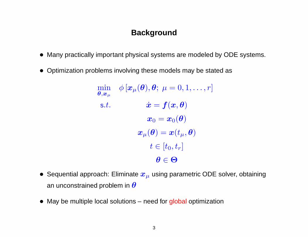
Background

• Many practically important physical systems are modeled by ODE systems.

• Optimization problems involving these models may be stated as

minθ,xµ

φ [xµ(θ), θ; µ = 0, 1, . . . , r]

s.t. x = f(x, θ)

x0 = x0(θ)

xµ(θ) = x(tµ, θ)

t ∈ [t0, tr]

θ ∈ Θ

• Sequential approach: Eliminate xµ using parametric ODE solver, obtaining

an unconstrained problem in θ

• May be multiple local solutions – need for global optimization

3

Deterministic Global Optimization of Dynamic Systems

Much recent interest, mostly combining branch-and-bound and relaxation

techniques, e.g.,

• Esposito and Floudas (2000): α-BB approach

– Rigorous values of α not used: no theoretical guarantees

• Chachuat and Latifi (2003): Theoretical guarantee of ε-global optimality

• Papamichail and Adjiman (2002, 2004): Theoretical guarantee of ε-global

optimality

• Singer and Barton (2006): Theoretical guarantee of ε-global optimality

– Use convex underestimators and concave overestimators to construct two

bounding IVPs, which are then solved to obtain lower and upper bounds

on the state trajectories.

– Bounding IVPs are not solved rigorously, so state bounds are not

computationally guaranteed.

4

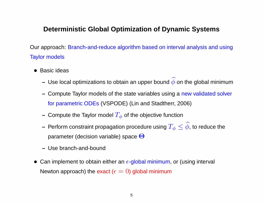
Deterministic Global Optimization of Dynamic Systems

Our approach: Branch-and-reduce algorithm based on interval analysis and using

Taylor models

• Basic ideas

– Use local optimizations to obtain an upper bound φ on the global minimum

– Compute Taylor models of the state variables using a new validated solver

for parametric ODEs (VSPODE) (Lin and Stadtherr, 2006)

– Compute the Taylor model Tφ of the objective function

– Perform constraint propagation procedure using Tφ ≤ φ, to reduce the

parameter (decision variable) space Θ

– Use branch-and-bound

• Can implement to obtain either an ε-global minimum, or (using interval

Newton approach) the exact (ε = 0) global minimum

5

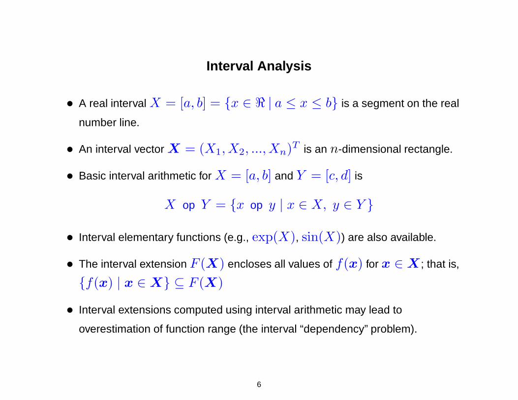
Interval Analysis

• A real interval X = [a, b] = {x ∈ < | a ≤ x ≤ b} is a segment on the real

number line.

• An interval vector X = (X1, X2, ..., Xn)T is an n-dimensional rectangle.

• Basic interval arithmetic for X = [a, b] and Y = [c, d] is

X op Y = {x op y | x ∈ X, y ∈ Y }

• Interval elementary functions (e.g., exp(X), sin(X)) are also available.

• The interval extension F (X) encloses all values of f(x) for x ∈ X ; that is,

{f(x) | x ∈ X} ⊆ F (X)

• Interval extensions computed using interval arithmetic may lead to

overestimation of function range (the interval “dependency” problem).

6

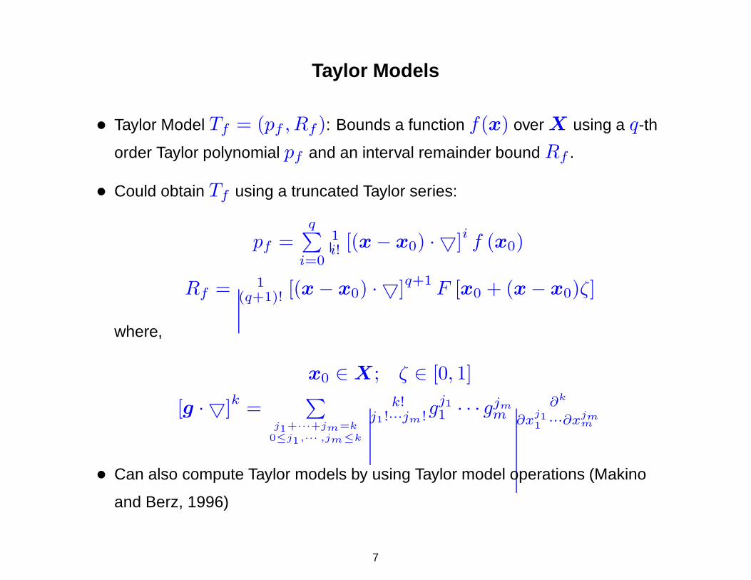
Taylor Models

• Taylor Model Tf = (pf , Rf ): Bounds a function f(x) over X using a q-th

order Taylor polynomial pf and an interval remainder bound Rf .

• Could obtain Tf using a truncated Taylor series:

pf =q∑

i=0

1i! [(x − x0) · 5]

if (x0)

Rf = 1(q+1)! [(x − x0) · 5]q+1 F [x0 + (x − x0)ζ]

where,

x0 ∈ X; ζ ∈ [0, 1]

[g · 5]k =∑

j1+···+jm=k

0≤j1,··· ,jm≤k

k!j1!···jm!g

j11 · · · gjm

m∂k

∂xj11 ···∂x

jmm

• Can also compute Taylor models by using Taylor model operations (Makino

and Berz, 1996)

7

Taylor Model Operations

• Let Tf and Tg be the Taylor models of the functions f(x) and g(x),

respectively, over the interval x ∈ X .

• Addition: Tf±g = (pf±g, Rf±g) = (pf ± pg, Rf ± Rg)

• Multiplication: Tf×g = (pf×g, Rf×g) with pf×g = pf × pg − pe and

Rf×g = B(pe) + B(pf ) × Rg + B(pg) × Rf + Rf × Rg

• B(p) indicates an interval bound on the function p.

• Reciprocal operation and intrinsic functions can also be defined.

• Store and operate on coefficients of pf only. Floating point errors are

accumulated in Rf .

• Beginning with Taylor models of simple functions, Taylor models of very

complicated functions can be computed.

• Compared to other rigorous bounding methods (e.g., interval arithmetic),

Taylor models often yield sharper bounds for modest to complicated

functional dependencies (Makino and Berz, 1999).

8

Taylor Models – Range Bounding

• Exact range bounding of the interval polynomials – NP hard

• Direct evaluation of the interval polynomials – overestimation

• Focus on bounding the dominant part (1st and 2nd order terms)

• Exact range bounding of a general interval quadratic – also worst-case

exponential complexity

• A compromise approach – Exact bounding of 1st order and diagonal 2nd

order terms

B(p) =m∑

i=1

[ai (Xi − xi0)

2 + bi(Xi − xi0)]

+ S

=

m∑

i=1

[ai

(Xi − xi0 +

bi

2ai

)2

− b2i

4ai

]+ S,

where S is the interval bound of other terms by direct evaluation

9

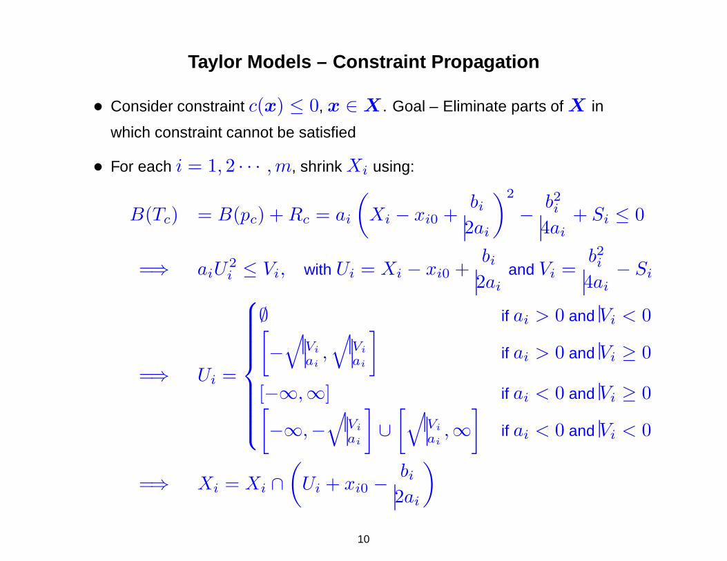
Taylor Models – Constraint Propagation

• Consider constraint c(x) ≤ 0, x ∈ X . Goal – Eliminate parts of X in

which constraint cannot be satisfied

• For each i = 1, 2 · · · , m, shrink Xi using:

B(Tc) = B(pc) + Rc = ai

(Xi − xi0 +

bi

2ai

)2

− b2i

4ai

+ Si ≤ 0

=⇒ aiU2i ≤ Vi, with Ui = Xi − xi0 +

bi

2ai

and Vi =b2i

4ai

− Si

=⇒ Ui =

∅ if ai > 0 and Vi < 0[−

√Vi

ai,√

Vi

ai

]if ai > 0 and Vi ≥ 0

[−∞,∞] if ai < 0 and Vi ≥ 0[−∞,−

√Vi

ai

]∪

[√Vi

ai,∞

]if ai < 0 and Vi < 0

=⇒ Xi = Xi ∩(

Ui + xi0 −bi

2ai

)

10

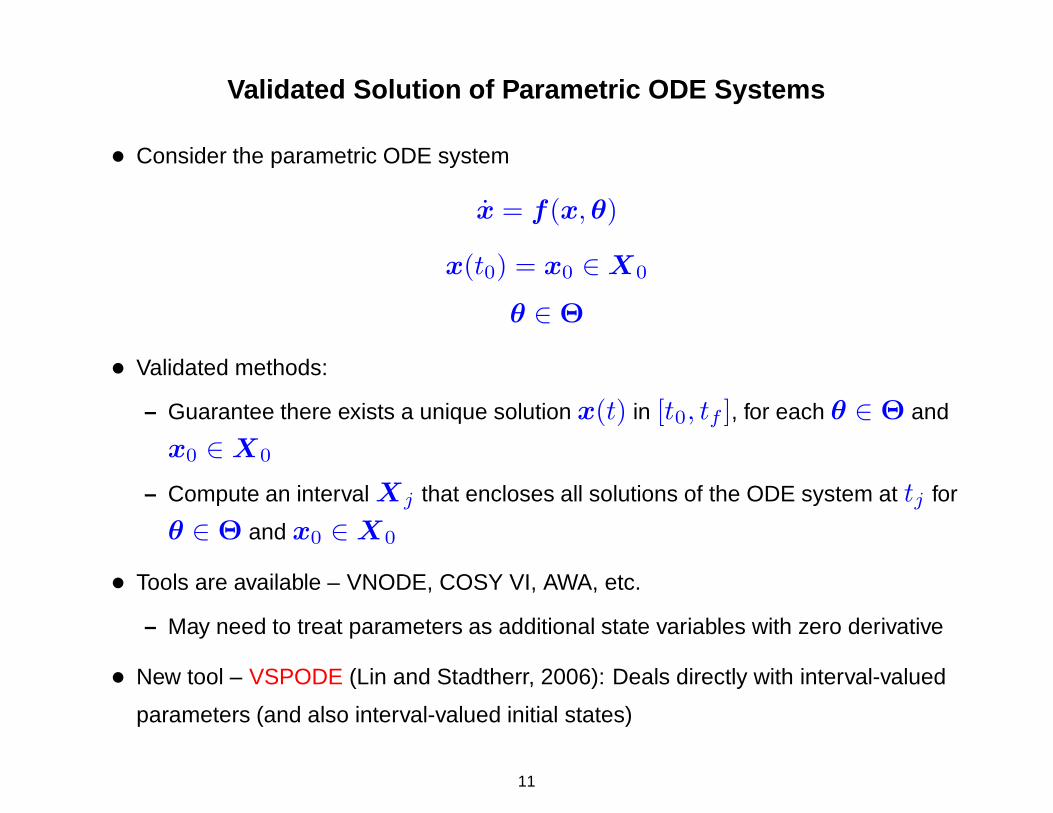
Validated Solution of Parametric ODE Systems

• Consider the parametric ODE system

x = f(x, θ)

x(t0) = x0 ∈ X0

θ ∈ Θ

• Validated methods:

– Guarantee there exists a unique solution x(t) in [t0, tf ], for each θ ∈ Θ and

x0 ∈ X0

– Compute an interval Xj that encloses all solutions of the ODE system at tj for

θ ∈ Θ and x0 ∈ X0

• Tools are available – VNODE, COSY VI, AWA, etc.

– May need to treat parameters as additional state variables with zero derivative

• New tool – VSPODE (Lin and Stadtherr, 2006): Deals directly with interval-valued

parameters (and also interval-valued initial states)

11

New Method for Parametric ODEs

• Use interval Taylor series to represent dependence on time. Use Taylor

models to represent dependence on uncertain quantities (parameters and

initial states).

• Assuming Xj is known, then

– Phase 1: Same as “standard” approach (e.g., VNODE). Compute a coarse

enclosure Xj and prove existence and uniqueness. Use fixed point

iteration with Picard operator using high-order interval Taylor series.

– Phase 2: Refine the coarse enclosure to obtain Xj+1. Use Taylor models

in terms of the uncertain parameters and initial states.

• Implemented in VSPODE (Validating Solver for Parametric ODEs) (Lin and

Stadtherr, 2006).

12

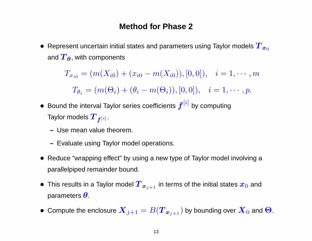
Method for Phase 2

• Represent uncertain initial states and parameters using Taylor models T x0

and T θ , with components

Txi0 = (m(Xi0) + (xi0 − m(Xi0)), [0, 0]), i = 1, · · · , m

Tθi= (m(Θi) + (θi − m(Θi)), [0, 0]), i = 1, · · · , p.

• Bound the interval Taylor series coefficients f [i] by computing

Taylor models T f [i] .

– Use mean value theorem.

– Evaluate using Taylor model operations.

• Reduce “wrapping effect” by using a new type of Taylor model involving a

parallelpiped remainder bound.

• This results in a Taylor model T xj+1 in terms of the initial states x0 and

parameters θ.

• Compute the enclosure Xj+1 = B(T xj+1) by bounding over X0 and Θ.

13

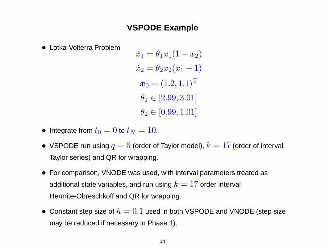
VSPODE Example

• Lotka-Volterra Problemx1 = θ1x1(1 − x2)

x2 = θ2x2(x1 − 1)

x0 = (1.2, 1.1)T

θ1 ∈ [2.99, 3.01]

θ2 ∈ [0.99, 1.01]

• Integrate from t0 = 0 to tN = 10.

• VSPODE run using q = 5 (order of Taylor model), k = 17 (order of interval

Taylor series) and QR for wrapping.

• For comparison, VNODE was used, with interval parameters treated as

additional state variables, and run using k = 17 order interval

Hermite-Obreschkoff and QR for wrapping.

• Constant step size of h = 0.1 used in both VSPODE and VNODE (step size

may be reduced if necessary in Phase 1).

14

Lotka-Volterra Problem

0 1 2 3 4 5 6 7 8 9 100.5

0.6

0.7

0.8

0.9

1

1.1

1.2

1.3

1.4

1.5

t

x

← X1

← X2

VSPODEVNODE

(Eventual breakdown of VSPODE at t = 31.8)

15

Summary of Global Optimization Algorithm

Beginning with initial parameter interval Θ(0)

• Establish φ, the upper bound on global minimum using p2 local

minimizations, where p is the number of parameters (decision variables)

• Iterate: for subinterval Θ(k)

1. Compute Taylor models of the states using VSPODE, and then obtain Tφ

2. Perform constraint propagation using Tφ ≤ φ to reduce Θ(k)

3. If Θ(k) = ∅, go to next subinterval

4. If (φ − B(Tφ))/|φ| ≤ εrel, or φ − B(Tφ) ≤ εabs, discard Θ(k) and

go to next subinterval

5. If B(Tφ) < φ, update φ with local minimization, go to step 2

6. If Θ(k) is sufficiently reduced, go to step 1

7. Otherwise, bisect Θ(k) and go to next subinterval

• This finds an ε-global optimum with either a relative tolerance (εrel) or

absolute tolerance (εabs)

16

Global Optimization Algorithm (cont’d)

• By incorporating an interval-Newton approach, this can also be implemented

as an exact algorithm (ε = 0).

• This requires the validated integration of the first- and second-order sensitivity

equations. VSPODE was used.

• Interval-Newton steps are applied only after reaching an appropriate depth in

the branch-and-bound tree

• We have implemented the exact algorithm only for the case of parameter

estimation problems with least squares objective

• The exact algorithm may require more or less computation time than the

ε-global algorithm

17

Computational Studies – Example 1

• Parameter estimation – Catalytic cracking of gas oil (Tjoa and Biegler 1991)

Aθ1

θ3

Q

θ2

S

• The problem is:

minθ

φ =20∑

µ=1

2∑

i=1

(xµ,i − xµ,i)2

s.t. x1 = −(θ1 + θ3)x21

x2 = θ1x21 − θ2x2

x0 = (1, 0)T; xµ = x(tµ)

θ ∈ [0, 20] × [0, 20] × [0, 20]

where xµ is given (experimental data).

18

Example 1 (Cont’d)

• Solution: θ∗ = (12.2139, 7.9798, 2.2217)T and φ∗ = 2.6557 × 10−3

• Comparisons:

CPU time (s)

Method Reported Adjusted∗

This work (exact global optimum: ε = 0) 11.5 11.5(Intel P4 3.2GHz)

This work (εrel = 10−3) 14.3 14.3(Intel P4 3.2GHz)

Papamichail and Adjiman (2002) (εrel = 10−3) 35478 4541(SUN UltraSPARC-II 360MHz)

Chachuat and Latifi (2003) (εrel = 10−3) 10400 −(Machine not reported)

Singer and Barton (2006) (εabs = 10−3) 5.78 2.89(AMD Athlon 2000XP+ 1.667GHz)

∗Adjusted = Approximate CPU time after adjustment for machine used (based on SPEC benchmark)

19

Computational Studies – Example 2

• Singular control problem (Luus, 1990)

• The original problem is stated as:

minθ(t)

φ =

∫ tf

t0

[x2

1 + x22 + 0.0005(x2 + 16t − 8 − 0.1x3θ

2)2dt]

s.t. x1 = x2

x2 = −x3θ + 16t − 8

x3 = θ

x0 = (0,−1,−√

5)T

t ∈ [t0, tf ] = [0, 1]

θ ∈ [−4, 10]

• θ(t) is parameterized as a piecewise constant control profile with n pieces

(equal time intervals)

20

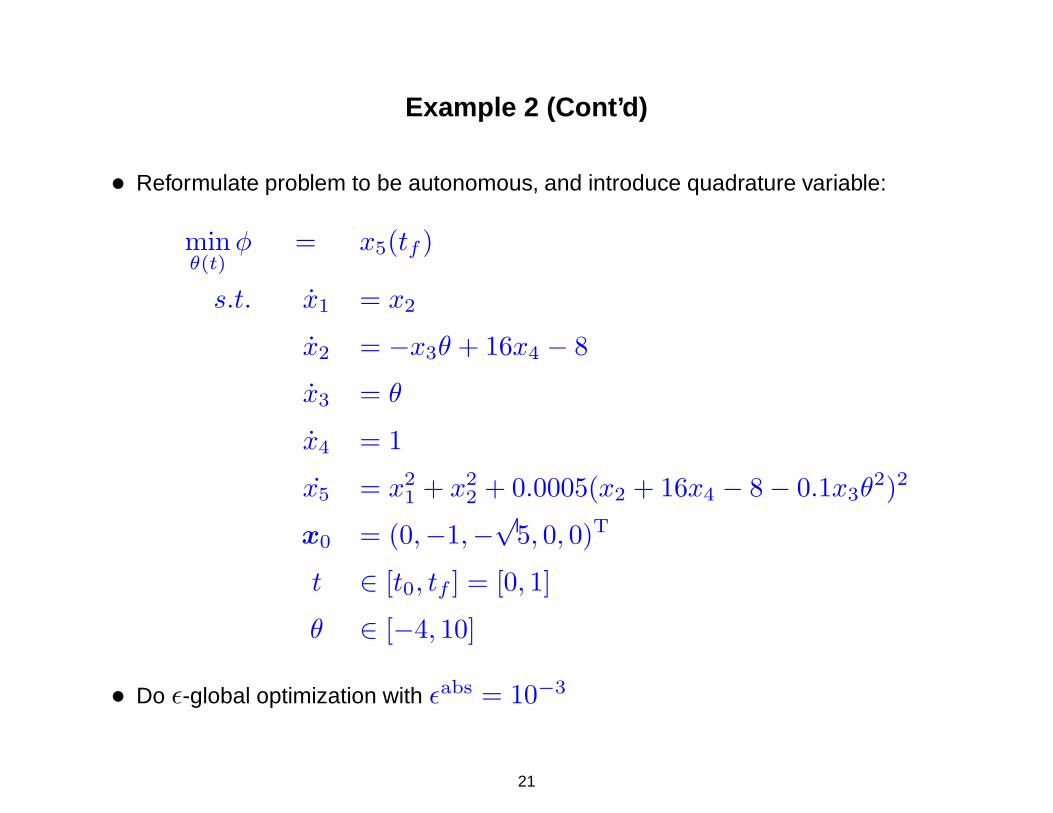
Example 2 (Cont’d)

• Reformulate problem to be autonomous, and introduce quadrature variable:

minθ(t)

φ = x5(tf )

s.t. x1 = x2

x2 = −x3θ + 16x4 − 8

x3 = θ

x4 = 1

x5 = x21 + x2

2 + 0.0005(x2 + 16x4 − 8 − 0.1x3θ2)2

x0 = (0,−1,−√

5, 0, 0)T

t ∈ [t0, tf ] = [0, 1]

θ ∈ [−4, 10]

• Do ε-global optimization with εabs = 10−3

21

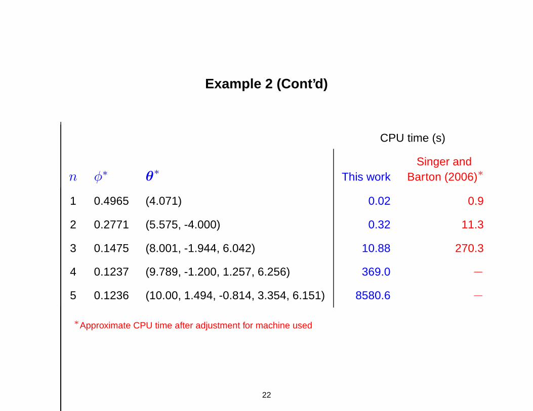
Example 2 (Cont’d)

CPU time (s)

Singer andn φ∗ θ∗ This work Barton (2006)∗

1 0.4965 (4.071) 0.02 0.9

2 0.2771 (5.575, -4.000) 0.32 11.3

3 0.1475 (8.001, -1.944, 6.042) 10.88 270.3

4 0.1237 (9.789, -1.200, 1.257, 6.256) 369.0 −5 0.1236 (10.00, 1.494, -0.814, 3.354, 6.151) 8580.6 −∗Approximate CPU time after adjustment for machine used

22

Computational Studies – Example 3

• Oil shale pyrolysis problem (Luus, 1990)

• The original problem is stated as:

minθ(t)

φ = −x2(tf )

s.t. x1 = −k1x1 − (k3 + k4 + k5)x1x2

x2 = k1x1 − k2x2 + k3x1x2

ki = ai exp

(−bi/R

θ

), i = 1, . . . , 5

x0 = (1, 0)T

t ∈ [t0, tf ] = [0, 10]

θ ∈ [698.15, 748.15].

• θ(t) is paramaterized as a piecewise constant control profile with n pieces

(equal time intervals)

23

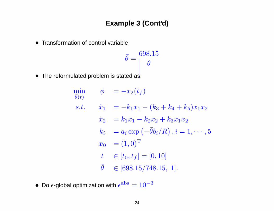
Example 3 (Cont’d)

• Transformation of control variable

θ =698.15

θ

• The reformulated problem is stated as:

minθ(t)

φ = −x2(tf )

s.t. x1 = −k1x1 − (k3 + k4 + k5)x1x2

x2 = k1x1 − k2x2 + k3x1x2

ki = ai exp(−θbi/R

), i = 1, · · · , 5

x0 = (1, 0)T

t ∈ [t0, tf ] = [0, 10]

θ ∈ [698.15/748.15, 1].

• Do ε-global optimization with εabs = 10−3

24

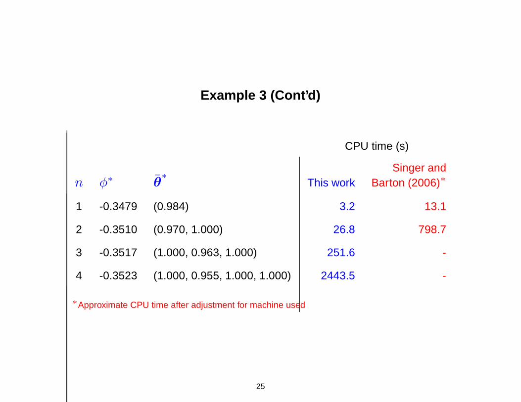
Example 3 (Cont’d)

CPU time (s)

Singer andn φ∗ θ

∗This work Barton (2006)∗

1 -0.3479 (0.984) 3.2 13.1

2 -0.3510 (0.970, 1.000) 26.8 798.7

3 -0.3517 (1.000, 0.963, 1.000) 251.6 -

4 -0.3523 (1.000, 0.955, 1.000, 1.000) 2443.5 -

∗Approximate CPU time after adjustment for machine used

25

Concluding Remarks

• An approach has been described for deterministic global optimization of

dynamic systems using interval analysis and Taylor models

– A validated solver for parametric ODEs is used to construct bounds on the

states of dynamic systems

– An efficient constraint propagation procedure is used to reduce the

incompatible parameter domain

• Can be combined with the interval-Newton method (Lin and Stadtherr, 2006)

– True global optimum instead of ε-convergence

– May or may not reduce CPU time required

26

Acknowledgments

• Indiana 21st Century Research & Technology Fund

• U. S. Department of Energy

27