Determining the Minimum Iteration Period of an Algorithm1

Kazuhito Itoy and Keshab K. Parhiz

yDepartment of Electrical and Electronic EngineeringTokyo Institute of TechnologyMeguro-ku, Tokyo 152, Japan

zDepartment of Electrical EngineeringUniversity of MinnesotaMinneapolis, MN 55455

E-mail: kazuhito@ss.titech.ac.jp, parhi@ee.umn.edu

Abstract — Digital signal processing algorithms are repetitive in nature. These algorithms are described

by iterative data-flow graphs where nodes represent computations and edges represent communications.

For all data-flow graphs, there exists a fundamental lower bound on the iteration period referred to as the

iteration bound. Determining the iteration bound for signal processing algorithms described by iterative

data-flow graphs is an important problem. In this paper we review two existing algorithms for determi-

nation of the iteration bound. Then we propose another novel method based on the minimum cycle mean

algorithm to determine the iteration bound with a lower polynomial time complexity than the two exist-

ing techniques. It is convenient to represent many multi-rate signal processing algorithms by multi-rate

data-flow graphs. The iteration bound of a multi-rate data-flow graph (MRDFG) can be determined by

considering the single-rate data-flow graph (SRDFG) equivalent of the MRDFG. However, the equiva-

lent single-rate data-flow graph contains many redundant nodes and edges. The iteration bound of the

MRDFG can be determined faster if these redundancies in the equivalent SRDFG are first removed. A

previous approach has considered elimination of edge redundancy. In this paper we present an approach

to eliminate node redundancy in the MRDFG. We combine elimination of node and edge redundancies

to propose a novel algorithm for faster determination of the iteration bound of the MRDFG.

1 Introduction

Digital signal processing algorithms are repetitive in nature. These algorithms are described by iterative data-flow

graphs (DFGs) where nodes represent tasks and edges represent communication [1, 2]. Execution of all nodes of the

DFG once completes an iteration. Successive iterations of any node are executed with a time displacement referred

1This research was supported by the Advanced Research Projects Agency and monitored by Wright - Patterson AFB under contract numberF33615-93-C-1309.

1

to as the iteration period. For all recursive signal processing algorithms, there exists an inherent fundamental lower

bound on the iteration period referred to as the iteration period bound or simply the iteration bound [3, 4, 5]. This

bound is fundamental to an algorithm and is independent of the implementation architecture. In other words, it is

impossible to achieve an iteration period less than the bound even when infinite processors are available to execute

the recursive algorithm.

Determination of the iteration bound of the data-flow graph is an important problem. First it discourages the

designer to attempt to design an architecture with an iteration period less than the iteration bound. Second, the iteration

bound needs to be determined in rate-optimal scheduling of iterative data-flow graphs. A schedule is said to be rate-

optimal if the iteration period is same as the iteration bound, i.e., the schedule achieves the highest possible rate of

operation of the algorithm.

The iteration bound determination may have to be performed repeatedly in the scheduling phase of high-level

synthesis. In resource-constrained scheduling, a given processing algorithm is scheduled to achieve the minimum

iteration period using the given hardware resources. In order to execute operations of the processing algorithm in

parallel, the required number of processors or functional units required to execute the operations in parallel may be

larger than the number of available resources. In that case, we must give the order of executions, or the precedence, to

these operations to reduce the parallelism. Generally the precedence to be assigned is not unique. Then the iteration

bound should be determined for every possible precedence to check which precedence leads to the final schedule with

the minimum iteration period. In this case, the iteration bound may have to be computed many times and hence it is

important to determine the iteration bound in minimum possible time.

Two algorithms have been recently proposed to determine the iteration bound. A method based on the negative

cycle detection was reported in [6] to determine the iteration bound with polynomial time complexity with respect to

the number of nodes in the processing algorithm. Another method based on the first-order longest path matrix was

proposed in [7] to determine the lower bound with polynomial time complexity with respect to the number of delays

in the processing algorithm. In this paper, based on [8], we propose yet another method based on the minimum cycle

mean algorithm [9] to determine the iteration bound with lower polynomial time complexity than in [6] and [7].

Several multi-rate signal processing algorithms can be conveniently represented by multi-rate data-flow graphs

[2]. To balance production and consumption of data on communicating edges between computations, the nodes of the

multi-rate data-flow graph need to be executed different number of times in any iteration of the MRDFG. Sufficient

theory to determine how many times a node in the MRDFG needs to be executed in an iteration has been developed

in [2]. All MRDFGs can be reduced to equivalent unform or single-rate DFGs (SRDFGs). The iteration bound of the

MRDFG can be determined by considering the equivalent SRDFG. However, the equivalent SRDFG contains many

redundancies with respect to nodes and edges. The iteration bound of the MRDFG can be determined faster if these

redundancies are first eliminated. An approach to determine the iteration bound by eliminating the edge degeneracy

has been proposed in [10]. In this paper we propose an approach to eliminate node redundancies. Then we present

2

an algorithm to determine the iteration bound in the MRDFGs in a faster manner by eliminating both edge and node

redundancies.

This paper is organized as follows. In section 2, the iteration bound is defined. The two existing algorithms

to determine the iteration bound are reviewed in section 3. Section 4 presents our new algorithm to determine the

iteration bound based on the minimum cycle-mean algorithm. The multi-rate DFG model is reviewed in section 5 and

an algorithm to determine the iteration bound in MRDFGs is introduced in section 6. The execution times of existing

and proposed algorithms to determine the iteration bound are compared in section 7 for a few benchmark algorithms.

2 Data-Flow Graph and the Iteration Bound

A data-flow graph (DFG) is denoted as G = (N;E; q; d) where N is the set of nodes, E is the set of directed edges, q

is the set of execution times of the nodes, and d is the set of delay counts associated with the edges. A directed path in

a DFG contains a series of connected edges. If the start node and the end node of a directed path are identical and no

node except the start node appears more than once in the path, the directed path is called a cycle (also often referred to

as a loop). Let C denote the set of all cycles of the DFG and Nc

be the set of nodes which belong to the cycle c. The

computation time of a cycle is defined as the sum of computation times of the nodes in the cycle. The delay count of

a cycle is defined as the sum of delay counts of the edges of the cycle. Let Mc

and Dc

denote the computation time

and the delay count of cycle c, respectively. These are calculated as

M

c

=X

i2N

c

q(i); (1)

D

c

=X

e2c

d(e): (2)

Let T denote the iteration period of the DFG. The DFG receives new data samples every T units of time and the

computation of each node is executed repetitively and periodically every T units of time. Smaller iteration period

implies faster processing. However, there exists a lower bound on the iteration period. It depends on the computation

time of nodes which belong to cycles and the data dependencies among them. For each cycle c, Mc

must be smaller

than or equal to D

c

T since all the computations of the nodes in c must be completed within D

c

T units of time.

Therefore, there exists a lower bound on the iteration period T due to cycle c. It is called the cycle bound and the

cycle bound Tc

is calculated as

T

c

=M

c

D

c

: (3)

The lower bound on the iteration period is the maximum of the cycle bounds. This is referred to as the iteration bound,

T

i

, and is calculated as

T

i

= maxc2C

T

c

= maxc2C

M

c

D

c

: (4)

A critical cycle is defined as the cycle c whose cycle bound equals the iteration bound.

3

We assume that the DFG is a strongly connected graph. A strongly connected graph is a graph such that there exists

a directed path between any pair of nodes. If the DFG is not strongly connected, we can derive strongly connected

components with the computational complexityO(jN j+ jEj) [11], where jN j and jEj are the number of nodes and the

number of edges, respectively, and determine the iteration bound for each component. Then, the maximum of these

iteration bounds is the iteration bound of the DFG.

3 Previous Work on Iteration Bound Determination

In this section, two previously proposed methods of determination of the iteration bound for a given DFG are reviewed.

3.1 The negative cycle detection method

An algorithm to determine the iteration bound based on the negative cycle detection method [12] has been recently

proposed in [6, 10]. A negative cycle is a cycle where the sum of weights of edges on the cycle is negative.

Given the DFG, G = (N;E; q; d), and the guess value of the iteration bound T0, an edge-weighted digraph

G = (N;E; w) is constructed. The node set and the edge set of G are exactly the same as N and E, respectively,

and the weight w(e) of edge e = (u; v)(2 E) is given by w(e) = d(e)T0 � q(u). A shortest path algorithm can be

executed on this graph to check presence of any negative cycle. We can use the well-known shortest path algorithm

such as Floyd method which requires the time complexity O(jN j3) or Bellman-Ford method which requires the time

complexity O(jN jjEj) in the case when jEj is smaller than jN j2.

If the shortest path algorithm terminates without finding a solution, then there exists a negative cycle c where

X

e2c

w(e) = D

c

T0 �M

c

< 0: (5)

It means that the guess iteration bound T0 is smaller than the cycle bound Tc

= M

c

=D

c

and therefore than the true

iteration bound Ti

. On the other hand, if the shortest path algorithm terminates with a solution, then T0 is greater than

or equal to Ti

.

Thus, we increase the guess iteration period T0 if a negative cycle is detected or decrease it otherwise and re-

evaluate the weight of edges of G and repeat the shortest path algorithm. By using a binary-search technique to

determine the amount by which T0 is increased or decreased, the above procedure terminates with the result T0 = T

i

after O(log jN j) repetitions [12].

Therefore, the overall time complexity to determine the iteration bound is O(jN j3 log jN j) [6] or

O(jN jjEj log jN j). (However, it is claimed in [10] that O(jEj) = O(jN j) in ordinary DFGs and therefore the time

complexity is O(jN j2 log jN j).) The memory requirement is O(jN j2) when Floyd method is used, or O(jN j + jEj)

when Bellman-Ford method is used as the shortest path algorithm.

4

h j l

mk

i

D

2D

D

αβγ

δ

(1)

(1)

(1)

(2)

(2)

(4)

α β

γδ

7

5

4

016

3 α β

γδ

0

−3

−6 −1

−7

−5

−4

(a) (b) (c)

G=(N,E,q,d)

N={h,i,j,k,l,m}

Gd=(D,Ed,w)

D=(α,β,γ,δ)

Gd=(D,Ed,w)

D=(α,β,γ,δ)

Fig. 1. The DFG G and the corresponding edge-weighted digraph Gd

. In parenthesis in G are the computation timesof nodes.

3.2 The longest path matrix method

Another technique to determine the iteration bound of the given DFG by using the first-order longest path matrix was

proposed in [7].

From the DFG G = (N;E; q; d), an edge-weighted digraph G

d

= (D;E

d

; w) is constructed. Fig. 1 illustrates

an original DFG and the constructed graph corresponding to the DFG. D is the set of nodes which is a delay in the

original graph G. Therefore, a delay in the graph G corresponds to a node in the graph G

d

. If a directed path in G

consists of edges with no delay except the first and last edges, an edge spanning a pair of nodes in D corresponding

to these two delays is included in the edge set Ed

. There is such a directed path (k; h), (h; i), (i; l) in Fig. 1(a) and an

edge (�; �) is included in Ed

, since � and � are delays on the first edge (k; h) and the last edge (i; l), respectively.

We define path length in this paper as the sum of computation time of the intermediate nodes on the path. The

length of the path stated above is the sum of computation time of the nodes h and i. The weight of the edge e 2 E

d

,

w(e), is equal to the length of the path corresponding to the edge e. In Fig. 1(a), there is a path from the delay labeled

as � to itself, with the intermediate nodes j and h. The weight w(�; �) is the sum of computation times of j and h,

i.e., 3. In this case, the edge forms a self cycle as shown in Fig. 1(b). In general, multiple paths may exist between

two delays. Then, the weight of the edge is set to the longest path length among these paths. For example, between

delays labeled as � and � in Fig. 1(a), there are two directed paths which go through nodes j, m, k and j, l, m, k. The

lengths of these paths are 5 and 6, respectively. Thus, the weight w(�; �) is set to 6.

If more than one delay elements exist on an edge in G, then more than one node is included in the node set D.

The weight of the edge between the nodes corresponding to these delays is 0 since there exists no computation node

between these delays. In Fig. 1, there are two delays on the edge (i; j) in G and these correspond to the two nodes �

and in Gd

. The edge (�; ) is included in Ed

and the weight w(�; ) is 0.

The first-order longest path matrix L

1 is a jDj � jDj matrix and its element l1ij

is equal to the weight w(i; j) of

the edge (i; j) of Gd

or �1 if such an edge does not exist. The element lk+1ij

of the longest path matrix of the order

5

k(> 0) is recursively defined as

l

k+1ij

= maxn2D

n

l

1in

+ l

k

nj

o

: (6)

The diagonal element lkii

ofLk is the longest computation time among cycles which contains exactly k nodes including

the node i. Since a node in Gd

represents a delay in G, the maximum of lkii

for all i corresponds to the longest cycle

in G containing exactly k delays. Therefore,

T = max1�k�jDj

maxi

l

k

ii

k

(7)

is the largest cycle bound of all the cycles and is the iteration bound of the DFG, G.

From the DFG G = (N;E; q; d), the weighted digraph G

d

= (D;E

d

; w) and L

1 are constructed in O(jDjjEj)

computational time. The time complexities to compute maxi

l

k

ii

and L

k+1 from L

k are O(jDj) and O(jDj3), respec-

tively. These computations are repeated jDj times for 1 � k � jDj. Hence, the total computational complexity is

O((jDj + jDj3)jDj + jDjjEj) = O(jDj4 + jDjjEj) [7].

If we construct an edge-weighted digraph G

d

= (D;E

d

; w) where the weight of an edge e 2 E

d

is given by

w(e) = T0 � w(e) where T0 is a guess iteration bound, then the technique mentioned in the previous section can be

used to determine the iteration bound. From the DFG G = (N;E; q; d), constructing G

d

= (D;Ed

; w) requires the

computation time ofO(jDjjEj) complexity. The computation time to determine the iteration bound of Gd

by using Gd

is the complexity of O(jDj3 log jDj). Hence, the total time complexity is O(jDj3 log jDj + jDjjEj) [7]. The memory

requirement is O(jN j + jDj2) for calculating L1 and storing Lk.

The methods described in this section would be faster than the method based on the negative cycle detection where

the number of delays jDj is relatively smaller than the number of nodes jN j and the number of edges jEj.

4 A New Algorithm to Determine the Iteration Bound

In this section, we propose an algorithm to determine the iteration bound by using the minimum cycle mean algorithm.

The cycle mean of a cycle c, m(c), is defined as

m(c) =P

e2c

w(e)p

c

(8)

where w(e) is the weight of the edge e and pc

is the number of edges in cycle c. In other words, the cycle mean of a

cycle c is average weight of the edges included in c.

The minimum cycle mean problem involves the determination of the minimum cycle mean, �, of all the cycles in

the given digraph where

� = minc

m(c): (9)

An efficient algorithm was proposed in [9] to determine the minimum cycle mean for a given graph with time com-

plexity O(jN jjEj), where N and E are the set of nodes and the set of edges of the graph, respectively.

6

j lk

iDα

β (1)(2)

α β

5

1

(a) (b)

D

(1)

(2)

Fig. 2. The cycle mean and the cycle bound.

The number of nodes in a cycle is equal to the number of edges of the cycle. According to the definition of the

graph G

d

= (D;E

d

; w), each node in G

d

corresponds to a delay in the DFG, G, and the edge weight w(d1; d2) of

the edge (d1; d2) 2 E

d

is the largest weight among all the paths from the delay d1 to the delay d2. Therefore, the

cycle mean of the cycle cd

, containing k nodes, d1, d2, . . ., dk

, is the maximum cycle bound of the cycles of G, which

contain the delays labeled d1, d2, . . ., dk

. For example, in the graph shown in Fig. 2(a), there are two delays labeled

� and �, respectively. There exist two cycles f(l; k); (k; i); (i; l)g and f(l; k); (k; j); (j; i); (i; l)g, both of which go

through delays � and �. Their cycle bounds are 4=2 = 2 and 6=2 = 3, respectively, and the maximum of them is 3.

Fig. 2(b) shows the graph G

d

= (D;E

d

; w) corresponding to the graph shown in Fig. 2(a). In Fig. 2(b), D = f�; �g,

w(�; �) = 1, and w(�; �) = 5. There exists one cycle f(�; �); (�; �)g and its cycle mean is 3. It equals the maximum

cycle bound of the cycles in the graph shown in Fig. 2(a), which contain the delays � and �.

Since the cycle mean of a cycle c in the graph G

d

equals the maximum cycle bound of the cycles in G which

contain the delays in cycle c, the maximum cycle mean of the graph G

d

equals the maximum cycle bound of all the

cycles in the graph G. Therefore, the iteration bound of the graph G can be obtained as the maximum cycle mean of

the graph Gd

.

Let Cd

denote the set of cycles in graph Gd

. Then, the maximum cycle mean of the graph G

d

is

maxc2C

d

m(c) = maxc2C

d

P

e2c

w(e)p

c

= maxc2C

d

�

P

e2c

(�w(e))p

c

= � minc2C

d

P

e2c

(�w(e))p

c

: (10)

It is the negative of the minimum cycle mean of the graph G

d

= (D;E

d

; w), where w(e) = �w(e) for every edge

e 2 E

d

. Consequently, the maximum cycle mean of the graph G

d

, i.e., the iteration bound of the graph G, can be

obtained as the negative of the minimum cycle mean of the graph Gd

.

The algorithm to determine the iteration bound of the given graph by means of the minimum cycle mean is

summarized in Fig. 3.

From the DFGG = (N;E; q; d), constructingGd

= (D;E

d

; w) and Gd

= (D;E

d

; w) requires the computation time

of O(jDjjEj) complexity. The time complexity to calculate the minimum cycle mean for the graph G

d

= (D;E

d

; w)

is O(jDjjEd

j). Hence, the total time complexity to determine the iteration bound is O(jDjjEd

j + jDjjEj). This

time complexity is better than the O(jDj3 log jDj + jDjjEj) complexity of the method described in section 3.2 since

jE

d

j � jDj

2 and therefore jEd

j � jDj

2 log jDj always holds. The memory requirement for calculating the edge

7

Input: DFG G = (N;E; q; d).Output: The iteration bound T

i

.1. Construct the graph G

d

= (D;E

d

; w) from the given DFG G = (N;E; q; d).2. Run the minimum cycle mean algorithm on G

d

.Minimum cycle mean algorithm2.0 Choose one node s 2 D arbitrarily.2.1 Calculate the minimum weight F

k

(v) of an edge progressionof length k from s to v as

F

k

(v) = min(u;v)2E

d

fF

k�1(u) + w(u; v)g for k = 1; 2; . . . ; jDj

with the initial conditions F0(s) = 0; F0(v) = 1, v 6= s.2.2 Calculate the minimum cycle mean � of G

d

.

� = minv2D

max0�k�jDj�1

F

jDj

(v) � F

k

(v)

jDj � k

3. Now, Ti

= �� is the iteration bound of the DFG G.

Fig. 3. The algorithm to determine the iteration bound.

weightw and determining the minimum cycle mean for the graph Gd

areO(jN j) andO(jDj2), respectively. The total

memory requirement is O(jN j + jDj2).

Example. From the given DFG G illustrated in Fig. 1(a), the edge-weighted digraph G

d

and G

d

are constructed

as shown in Fig. 1(b) and (c), respectively. If we choose � as s used in the minimum cycle mean algorithm, Fk

(v),

the minimum weight of paths consisting of exactly k edges in E

d

, and max0�k�jDj�1F

jDj

(v)�Fk

(v)jDj�k

are calculated as

follows:k

F

k

(v) 0 1 2 3 4 max0�k�3

F4(v) � F

k

(v)4� k

� 0 �3 �7 �10 �14 �3:5v � 1 �7 �11 �14 �18 �3:5

1 1 �7 �11 �14 �3� 1 �6 �9 �13 �16 �3

(11)

Then, � = minv2D

max0�k�jDj�1F

jDj

(v)�Fk

(v)jDj�k

= �3:5 and the iteration bound of the DFG G is 3.5. The reader may

confirm that the critical cycle is f(h; j); (j; l); (l; m); (m; k); (k; h)g and its cycle bound, that is the iteration bound

of the DFG, is 3.5 since the sum of computation times of nodes h; j; l;m; k is 7, the critical cycle contains 2 delays

labeled as � and �, and 7=2 = 3:5.

5 Multi-Rate Data-Flow Graph

While every node in a single rate data-flow graph (SRDFG) is invoked once in an iteration of the execution, nodes in

a multi-rate data-flow graph (MRDFG) are invoked more than once in an iteration. Moreover, different nodes may be

invoked for a different number of times in an iteration. In other words, one node is invoked at a different rate from

another node in MRDFGs. The definition of the edge in MRDFGs also differs from that in SRDFGs.

An MRDFG can be expanded into the equivalent SRDFG [1]. The ‘equivalence’ means that the MRDFG and its

expanded SRDFG express identical signal processing algorithm. In this section we describe a method to expand an

8

MRDFG into its equivalent SRDFG which is similar to unfolding an SRDFG [5].

5.1 The number of invocations of node

In SRDFGs, it is assumed that one invocation of a node consumes one data from every incoming edge and produces

one data on every outgoing edge. Therefore, the number of invocations of each node is one in an iteration. In

MRDFGs, on the other hand, one invocation of a node can consume one or more data from each incoming edge and

produce one or more data onto each outgoing edge. Let Ouv

and I

uv

denote the number of data produced onto the

edge (u; v) by an invocation of the node u and the number of data consumed from the edge (u; v) by an invocation of

the node v, respectively. They are written near the head and tail of the edge of the MRDFG as shown in Fig. 4(a). For

example, 4 data samples are produced onto the edge (a; b) in every invocation of the node a and 3 data samples are

consumed from the edge (a; b) in every invocation of the node b. In the case where O

uv

and I

uv

are different for the

directed edge (u; v), the node u must be invoked different number of times than the node v so that the total number

of data produced by the invocations of u and the total number of data consumed by the invocations of v balance

within each iteration. Let ku

denote the number of invocations of the node u in an iteration. Then, ku

and k

v

must

satisfy that Ouv

� k

u

= I

uv

� k

v

. These relations must be satisfied for every edge in the MRDFG. For example, in the

MRDFG shown in Fig. 4(a), there are four edges. The number of invocations ka

, kb

, and k

c

must satisfy the following

indeterminate equations:

4ka

= 3kb

(12)

k

b

= 2kc

(13)

3kc

= 2ka

(14)

k

c

= k

c

: (15)

By solving the set of equations with a constraint that at least two of the numbers of invocations are coprime to each

other, the minimum balanced numbers of invocations are 3, 4, and 2 for the nodes a, b, and c, respectively.

5.2 Edges in the equivalent single-rate DFG

The equivalent SRDFG contains k

u

nodes which are the k

u

copies of node u of the MRDFG. Since every node is

executed once in an iteration of the SRDFG, the total number of executions of the copies of node u in an iteration of

the equivalent SRDFG is the same as the number of executions of node u in an iteration of the MRDFG.

Edges are also copied in the equivalent SRDFG. Each invocation of the node u produces O

uv

data on the edge

(u; v) in the MRDFG. It can be emulated in the SRDFG by appending O

uv

copies of the edge (u; v) outgoing from

each copy of the node u. Since the execution of a copy of the node u produces one data on every outgoing edge,

the number of data produced by the execution is O

uv

. Similarly, Iuv

copies of the edge (u; v) are incoming to each

copy of the node v and total number of data consumed by the execution of a copy of the node v is I

uv

. There are

k

v

I

uv

(= k

u

O

uv

) copies of the edge (u; v).

9

a b c3D 2D

D

43

3

2

21 1

1

a0

a

a

0

2

b

b

b

b

1

2

3

0c

c1

1

DDD

D

D

D

(a) (b)

Fig. 4. An MRDFG and its equivalent SRDFG.

To simplify notation, in the remainder of this paper, let xny and x%y denotej

x

y

k

and x �

j

x

y

k

y, respectively,

where bzc is the largest integer less than or equal to z and x%y is x modulo y.

Let uk (k = 0; 1; . . . ; ku

� 1) denote the node in the equivalent SRDFG, which corresponds to the k-th invocation

of the node u of the MRDFG. Since O

uv

edges are outgoing from the node u

k, uk can be regarded as having O

uv

output terminals for the edge (u; v). Similarly, the node vk can be regarded as having I

uv

input terminals for the edge

(u; v). There are O

uv

k

u

output terminals on k

u

nodes u0; u

1; . . . ; uk

u

�1 and I

uv

k

v

(= O

uv

k

u

) input terminals on k

v

nodes v0; v

1; . . . ; vk

v

�1. Then, the i-th (i = 0; 1; . . . ; Ouv

k

u

� 1) copy of the edge connects the i-th output terminal

of the copies of the node u (it is the (i%O

uv

)-th terminal of the node uinOuv ) and the i-th input terminal of the copies

of the node v (it is the (i%I

uv

)-th terminal of the node vinIuv ) if there is no delay on the edge (u; v).

The delay on an edge in an SRDFG implies the inter-iteration data dependency, where the computation of the

current iteration depends on the data generated in the previous iteration. On the other hand, in the MRDFG, the delay

on an edge does not imply the inter-iteration data dependency. It is the offset between the output terminal and the

input terminal connected by a copy of the edge in the equivalent SRDFG. If the number of delays on the edge (u; v)

is W in the MRDFG, the i-th copy of the edge connects the i-th output terminal of the copies of u with the (i +W )-th

input terminal of the copies of v. Therefore, the i-th copy of the edge (u; v) is outgoing from the node u

inO

uv and

incoming to the node v(i+W )nIuv . In the case that (i + W )nI

uv

� k

v

, the edge is incoming to the node v((i+W )nIuv

)%k

v

and ((i + W )nIuv

)nkv

= (i + W )n(Iuv

k

v

) delays are associated with the edge. These delays now imply inter-iteration

data dependencies since they exist in the SRDFG.

Example. Fig. 4 shows an MRDFG and its equivalent SRDFG. The numbers of invocations of node a, b, and c are

3, 4, and 2, respectively. There are 12 copies of the edge (a; b) since Oab

= 4 and k

a

= 3. The edge (a; b) is associated

with 3 delays. Therefore, the 9th, 10th, and 11th copies of the edge, all incoming to b

0, are associated with one delay.

5.3 Constructing the equivalent SRDFG

The algorithm to construct the equivalent SRDFG for a given MRDFG is summarized in Fig. 5.

10

Input: MRDFG G

m

= (Nm

; E

m

; q

m

; d

m

)Output: SRDFG G

s

= (Ns

; E

s

; q

s

; d

s

)N

s

= Ø, Es

= Ø;Calculate k

u

for all u 2 Nm

;for all u 2 N

m

dofor k = 0 to k

u

� 1 doInclude uk into N

s

;q

s

(uk) q

m

(u)enddo

enddofor all (u; v) 2 E

m

doW d

m

(u; v).for i = 0 to O

uv

k

u

� 1 doInclude (uinOuv

; v

((i+W )nIuv

)%kv ) into E

s

;d

s

(uinOuv

; v

((i+W )nIuv

)%kv ) (i + W )n(I

uv

k

v

)enddo

enddo

Fig. 5. An algorithm to construct the equivalent SRDFG.

Construction of the equivalent SRDFG requires the computations of O(jNm

jk) complexity for generating N

s

and O(jEm

jk) complexity for generating Es

where k is the average of ku

for all u 2 N

m

. The total computational

complexity to construct the equivalent SRDFG is O((jNm

j + jEm

j)k).

6 The Iteration Bound of Multi-Rate DFG

The iteration bound of an MRDFG is identical to the iteration bound of the equivalent SRDFG since these express the

identical signal processing algorithm. Hence, the iteration bound of the MRDFG can be determined by determining

the iteration bound of the equivalent SRDFG. From the viewpoint of determining the iteration bound, however, the

equivalent SRDFG is redundant in the number of edges and the number of nodes in some cases. This kind of redun-

dancy immediately worsens the computation time to determine the iteration bound since it depends on the number of

nodes and the number of edges. The computation time to determine the iteration bound of the equivalent SRDFG may

be improved by eliminating these redundancies. In this section, the technique to eliminate the edge redundancy of the

equivalent SRDFG is discussed. Then, we propose a technique to eliminate the node redundancy of the equivalent

SRDFG.

6.1 Edge degeneration

One of the redundancy is the existence of parallel edges in the equivalent SRDFG. If we remove all the parallel

edges except one edge with the least delays, a simple DFG is obtained. Let this edge removal procedure be called

edge degeneration. Although the edge degeneration alters the signal processing algorithm, the iteration bound is

not changed before and after the edge degeneration. Fig. 6(a) and (b) show a SRDFG equivalent of the MRDFG in

11

a0

a

a

0

2

b

b

b

b

1

2

3

0c

c1

1

D

D

D

D

(a) (b)

a0

a

a

0

2

b

b

b

b

1

2

3

0c

c1

1

DDD

D

D

D

a0

a

a

0

2

b

b

0c

1

1

DD

D

c1

~

~

(c)

~

~

~

~

~

Fig. 6. Degeneration of the equivalent SRDFG. (a) The equivalent SRDFG. (b) The edge-degenerated equivalentSRDFG. (c) The node-degenerated equivalent SRDFG.

Fig. 4(a) and the edge-degenerated SRDFG, respectively. For example, there are three edges from the node a2 to the

node b0 in the equivalent SRDFG. These edges are degenerated into a single edge from a

2 to b0 as shown in Fig. 6(b).

O

uv

edges outgoing from the node uk are input to the (Ouv

u

k + W )-th to (Ouk

(uk + 1) � 1 + W )-th terminals

where W is the number of delays associated with the edge (u; v). The edges incoming to the same node v

j are

degenerated into a single edge. Therefore, there exist the degenerated edges outgoing from u

k and incoming to vj%k

v ,

j = ((Ouv

u

k + W )nIuv

), ((Ouv

u

k + W )nIuv

) + 1, . . ., (Ouv

(uk + 1) � 1 + W )nIuv

, with jnk

v

delays for each j.

The algorithm to construct the edge-degenerated SRDFG directly from the given MRDFG is summarized in Fig. 7.

The time complexity of the algorithm is O((jNm

j + jEm

j)k) where k is the average of ku

for all u 2 N

m

. The edge

degeneration technique was also reported in [10]2.

6.2 Node degeneration

Another redundancy in the equivalent SRDFG is the existence of nodes which could be degenerated into one node

without altering the iteration bound. For example in edge-degenerated SRDFG illustrated in Fig. 6(c), the edges

outgoing from the nodes b0 and b

1 are incoming to an identical node c1 and these edges are the only edges outgoing

from b

0 and b1. In this case, as shown in Fig. 6(b), we can merge b0 and b1 into a single node b0 with the computation

time identical to b0 (also identical to b1). Such a node b0 is called the degenerated node. The edges connected to either

b

0 or b1 in the original SRDFG are connected to the degenerated node b0 without changing the number of delays on

these edges. Furthermore, newly introduced parallel edges in the SRDFG are also degenerated. This procedure is

called node degeneration.

The node degeneration is carried out such that the iteration bound of the node-degenerated SRDFG is identical to

that of the original SRDFG. The node degeneration is proper if the iteration bound is unchanged before and after the

2The technique described in [10] can also eliminate some transitive edges and hence derives a reduced SRDFG with the less number ofedges than the edge-degenerated SRDFG.

12

Input: MRDFG G

m

= (Nm

; E

m

; q

m

; d

m

)Output: the edge-degenerated SRDFG G

s

= (Ns

; E

s

; q

s

; d

s

)N

s

= Ø, Es

= Ø;Calculate k

u

for all u 2 Nm

;for all u 2 N

m

dofor k = 0 to k

u

� 1 doInclude uk into N

s

.q

s

(uk) q

m

(u).enddo

enddofor all (u; v) 2 E

m

doW d

m

(u; v).for k = 0 to k

u

� 1 dofor j = (O

uv

k + W )nIuv

to (Ouv

(k + 1)� 1 + W )nIuv

doInclude (uk; vj%k

v ) into Es

;d

s

(uk; vj%k

v ) jnk

v

enddoenddo

enddo

Fig. 7. An algorithm to construct the edge-degenerated equivalent SRDFG.

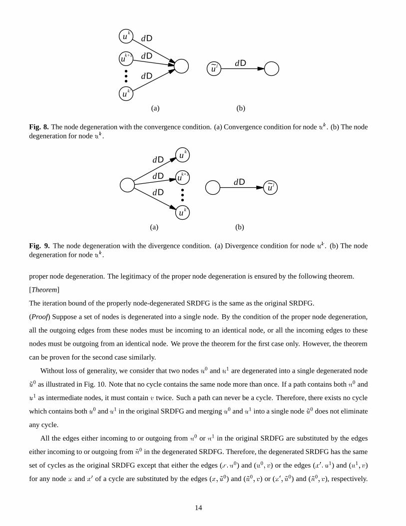
node degeneration. The node degeneration is proper in the case that either the convergence condition or the divergence

condition is satisfied. These conditions are defined as follows:

� Convergence condition (Fig. 8(a))

– The nodes to be degenerated into one degenerated node are the copies of a node of the MRDFG.

– The nodes have outgoing edges which are incoming to an identical node and are the only edges outgoing

from these nodes.

– The number of delays on the outgoing edges are the same.

� Divergence condition (Fig. 9(a))

– The nodes to be degenerated into one degenerated node are the copies of a node of the MRDFG.

– The nodes have incoming edges which are outgoing from an identical node and are the only edges incom-

ing to these nodes.

– The number of delays on the incoming edges are the same.

By the node degeneration with the convergence condition, the graph shown in Fig. 8(a) is degenerated as illustrated

in Fig. 8(b). Similarly, by the node degeneration with the divergence condition, the graph shown in Fig. 9(a) is

degenerated as illustrated in Fig. 9(b). For example in the SRDFG shown in Fig. 6(b), the nodes b0 and b

1 are the

copies of the node b of the MRDFG shown in Fig. 4(a), and all of their outgoing edges are incoming to the identical

node c1. Therefore, the convergence condition is satisfied and degenerating b

0 and b1 into a degenerated node b0 is a

13

(a)

u

u

u

k

k+1

k’

(b)

Dd

Dd

Ddu

Ddj~

Fig. 8. The node degeneration with the convergence condition. (a) Convergence condition for node u

k. (b) The nodedegeneration for node u

k.

(a) (b)

u

u

u

k

k+1

k’

Dd

Dd

Ddu

Dd j~

Fig. 9. The node degeneration with the divergence condition. (a) Divergence condition for node u

k. (b) The nodedegeneration for node u

k.

proper node degeneration. The legitimacy of the proper node degeneration is ensured by the following theorem.

[Theorem]

The iteration bound of the properly node-degenerated SRDFG is the same as the original SRDFG.

(Proof) Suppose a set of nodes is degenerated into a single node. By the condition of the proper node degeneration,

all the outgoing edges from these nodes must be incoming to an identical node, or all the incoming edges to these

nodes must be outgoing from an identical node. We prove the theorem for the first case only. However, the theorem

can be proven for the second case similarly.

Without loss of generality, we consider that two nodes u

0 and u

1 are degenerated into a single degenerated node

u

0 as illustrated in Fig. 10. Note that no cycle contains the same node more than once. If a path contains both u

0 and

u

1 as intermediate nodes, it must contain v twice. Such a path can never be a cycle. Therefore, there exists no cycle

which contains both u

0 and u

1 in the original SRDFG and merging u

0 and u

1 into a single node u

0 does not eliminate

any cycle.

All the edges either incoming to or outgoing from u

0 or u1 in the original SRDFG are substituted by the edges

either incoming to or outgoing from u

0 in the degenerated SRDFG. Therefore, the degenerated SRDFG has the same

set of cycles as the original SRDFG except that either the edges (x; u0) and (u0; v) or the edges (x0

; u

1) and (u1; v)

for any node x and x

0 of a cycle are substituted by the edges (x; u0) and (u0; v) or (x0

; u

0) and (u0; v), respectively.

14

u

(a) (b)

0

~u

1u v vx

x’x

x’

0

Fig. 10. Node degeneration. (a) A part of the original SRDFG. (b) The reduced SRDFG with u

0 and u1 merged intou

0.

Since u0 has the same computation time as u0 (and as u1) and the number of delays on (u0; v) is the same as (u0

; v)

and (u1; v), the maximum cycle bound of the degenerated SRDFG is identical to that of the original SRDFG. 2

6.3 Algorithm of node degeneration

By the node degeneration, the set of nodes uk (k = 0; 1; . . . ; ku

� 1) is degenerated into one or more nodes. Let

u

j (j = 0; 1; . . .) denote such degenerated nodes. The node degeneration is represented by the node degeneration

function, fu

(k) = j, which indicates that the node uk is degenerated into the node uj .

Suppose that node u

k1 is degenerated into the node u

j1 and node u

k2(k2 > k1) is degenerated into the node

u

j2 (j2 > j1) by the node-degeneration procedure mentioned above. Then, node uk3(k3 > k2) is degenerated either

into the node uj2 or into another node uj3(j3 > j2) by the node-degeneration procedure. It is important to note that

the node uk3 is never degenerated into the node uj1 if the node uk2 is not degenerated into uj1 . Consequently, the node

degeneration function is monotonically increasing function, i.e., fu

(k) � f

u

(k+1) for any node u and 0 � k � k

u

�1.

Deriving the node degeneration functions which lead to a properly node-degenerated SRDFG with the least num-

ber of nodes is the main task in the node degeneration.

A. Determining node degeneration function

The node degeneration function for the case of the convergence condition is derived as follows. Deriving the node

degeneration function for the case of the divergence condition can be described in a similar way.

Suppose that the edge (u; v) withW delays is the only outgoing edge from the node u in the MRDFG. Furthermore,

the nodes u and v are invoked k

u

times and k

v

times, respectively. Hence, Ouv

k

u

= I

uv

k

v

. Assume that (Ouv

k

0 +

W )nIuv

= (Ouv

(k0 + 1)� 1 + W )nIuv

for a node uk0. In other words, all the edges outgoing from u

k

0are incoming

to a single node v((Ouv

k

0+W )nIuv

)%kv . Let j = (O

uv

k

0 + W )nIuv

. Thus, all the edges outgoing from u

k

0are incoming

to the node vj%kv .

If (Ouv

(k + 1) � 1 + W )nIuv

= j for a k(� k

0 + 1), that is, all the edges outgoing from the node uk are also

incoming to the node vj%kv , then the nodes uk

0and uk can be degenerated into the same node. Hence, f

u

(k) is set as

f

u

(k0) to indicate that the nodes uk0

and uk are degenerated into an identical degenerated node ufu(k0).

15

On the other hand, if (Ouv

(k + 1) � 1 + W )nIuv

6= j, then u

k has an outgoing edge incoming to the node v

j

0

other then v

j . In this case, fu

(k) is set as fu

(k0) + 1 to indicate that the nodes uk cannot be degenerated into the same

degenerated node as uk0.

More generally, the set of nodes v

k may have been degenerated. In that case, it is checked whether outgoing

edges are incoming to an identical degenerated node. First, k0 is chosen as the smallest number to satisfy f

v

((Ouv

k

0 +

W )nIuv

) = f

v

((Ouv

(k0 + 1)�1 +W )nIuv

), i.e., all the outgoing edges from u

k

0are incoming to the degenerated node

v

f

v

(((Ouv

k

u

+W )nIuv

)%kv

). Let fv

(((Ouv

k

u

+ W )nIuv

)%k

v

) = j. If fv

((Ouv

(k + 1)� 1 + W )nIuv

= j for a k � k

0 + 1,

then let fu

(k) = f

u

(k0) since all the edges outgoing from u

k are incoming to v

j and therefore uk can be degenerated

into the same degenerated node as uk0. Otherwise, let f

u

(k) = f

u

(k0) + 1.

It must be noted that there can be the case where the convergence condition and/or the divergence condition is

not satisfied for some node u. In that case, node u

k is degenerated into the node u

k for k = 0; 1; . . . ; ku

� 1 by the

node-degeneration procedure and no node degeneration is performed.

B. The order of deriving node degeneration functions

Although the node degeneration function can be derived for each node independent of the processing order of the

nodes, one order of the nodes to be processed may result in a node-degenerated SRDFG with less nodes than another.

If the set of nodes uk is degenerated into the degenerated node u

k, more copies of the edge (u; v) may be outgoing

from an identical degenerated node u

k. In that case, the possibility of degenerating the set of nodes v

k would be

increased and they could be degenerated into less number of degenerated nodes.

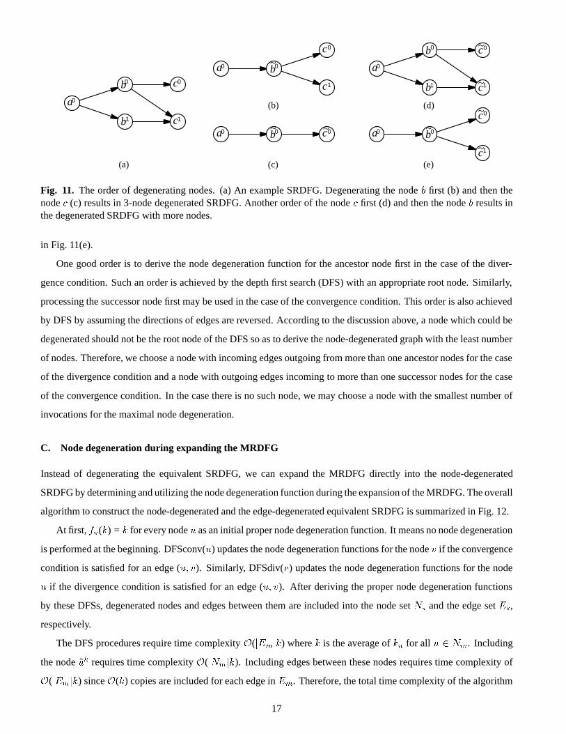
Fig. 11 shows an example. Let Fig. 11(a) be the equivalent SRDFG to be node-degenerated by the divergence

condition. The nodes b0 and b

1 satisfy the divergence condition since all the incoming edges to nodes b0 and b

1 are

outgoing from an identical node a

0 and there are no other edges incoming to nodes b0 and b

1. By applying the node

degeneration procedure on the node b, nodes b0 and b

1 are degenerated into a single degenerated node b

0 as shown in

Fig. 11(b). Then, nodes c0 and c

1 can be degenerated into a single degenerated node c

0 since all the incoming edges

to nodes c0 and c

1 are outgoing from an identical node b

0 and there are no other edges incoming to nodes c

0 and

c

1. Hence, the equivalent SRDFG shown in Fig. 11(a) is node-degenerated into the SRDFG shown in Fig. 11(c) by

applying the node degeneration procedure first on the node b and then on the node c.

If the node generation procedure is applied first on the node c, on the other hand, no actual node-degeneration

is performed on the nodes c

0 and c

1 since the convergence condition is not satisfied for the nodes c

0 and c

1. The

resultant SRDFG is illustrated in Fig. 11(d) and is identical to the original equivalent SRDFG. Then, applying the

node degeneration procedure on the node b results in the node-degenerated SRDFG shown in Fig. 11(e).

Consequently, applying the node degeneration procedure on the node b first and then the node c results in the

node-degenerated SRDFG with 3 nodes as shown in Fig. 11(c) and is better than applying the node degeneration

procedure on the node c first and then the node b which leads to the node-degenerated SRDFG with 4 nodes as shown

16

a0 0b

0c

c1

(a)

a

0

b

b

1

0c

c1

0

a

0

b

b

1

0~

a0 0b

0c

c1

~a0 0b 0c~ ~

~

~

0c

c1

~

~

(b)

(c)

(d)

(e)

Fig. 11. The order of degenerating nodes. (a) An example SRDFG. Degenerating the node b first (b) and then thenode c (c) results in 3-node degenerated SRDFG. Another order of the node c first (d) and then the node b results inthe degenerated SRDFG with more nodes.

in Fig. 11(e).

One good order is to derive the node degeneration function for the ancestor node first in the case of the diver-

gence condition. Such an order is achieved by the depth first search (DFS) with an appropriate root node. Similarly,

processing the successor node first may be used in the case of the convergence condition. This order is also achieved

by DFS by assuming the directions of edges are reversed. According to the discussion above, a node which could be

degenerated should not be the root node of the DFS so as to derive the node-degenerated graph with the least number

of nodes. Therefore, we choose a node with incoming edges outgoing from more than one ancestor nodes for the case

of the divergence condition and a node with outgoing edges incoming to more than one successor nodes for the case

of the convergence condition. In the case there is no such node, we may choose a node with the smallest number of

invocations for the maximal node degeneration.

C. Node degeneration during expanding the MRDFG

Instead of degenerating the equivalent SRDFG, we can expand the MRDFG directly into the node-degenerated

SRDFG by determining and utilizing the node degeneration function during the expansion of the MRDFG. The overall

algorithm to construct the node-degenerated and the edge-degenerated equivalent SRDFG is summarized in Fig. 12.

At first, fu

(k) = k for every node u as an initial proper node degeneration function. It means no node degeneration

is performed at the beginning. DFSconv(u) updates the node degeneration functions for the node v if the convergence

condition is satisfied for an edge (u; v). Similarly, DFSdiv(v) updates the node degeneration functions for the node

u if the divergence condition is satisfied for an edge (u; v). After deriving the proper node degeneration functions

by these DFSs, degenerated nodes and edges between them are included into the node set Ns

and the edge set Es

,

respectively.

The DFS procedures require time complexity O(jEm

jk) where k is the average of ku

for all u 2 N

m

. Including

the node uk requires time complexity O(jNm

jk). Including edges between these nodes requires time complexity of

O(jEm

jk) since O(k) copies are included for each edge in E

m

. Therefore, the total time complexity of the algorithm

17

Input: MRDFG G

m

= (Nm

; E

m

; q

m

; d

m

)Output: the node- and edge-degenerated SRDFG

G

s

= (Ns

; E

s

; q

s

; d

s

)N

s

=6 O, Es

= 6 O;Calculate k

u

for all u 2 Nm

;for all u 2 N

m

dofor k = 0 to k

u

� 1 dof

u

(k) k

enddoenddo/* Node degeneration for the convergence condition */for all u 2 N

m

doLabel u as ‘not processed’

enddoChoose the root node s for the convergence condition;call DFSconv(s);/* Node degeneration for the divergence condition */for all u 2 N

m

doLabel u as ‘not processed’

enddoChoose the root node s for the divergence condition;call DFSdiv(s);for all u 2 N

m

dofor k = 0 to f

u

(ku

� 1) doInclude uk into N

s

;q

s

(uk) q

m

(u)enddo

enddofor all (u; v) 2 E

m

doW d

m

(u; v);f

0 �1;

for k = 0 to ku

� 1 doif f

v

(((Ouv

(k + 1)� 1 + W )nIuv

)%k

v

) 6= f

0 thenf

0 f

v

(((Ouv

(k + 1)� 1 + W )nIuv

)%k

v

);j f

v

(((Ouv

k + W )nIuv

)%k

v

);W

0 (O

uv

k + W )n(Iuv

k

v

);if f0

� j then f

1 f

0

else f 1 f

0 + fv

(kv

� 1) + 1;for j1 = j to f 1 do

Include (ufu(k); v

j) into Es

;d

s

(ufu(k); v

j) W

0;j j + 1;if j > f

v

(kv

� 1) then j 0, W 0 W

0 + 1enddo

endifenddo

enddo.

procedure DFSconv(u)for all (u; v) 2 E

m

doif v is labeled as ‘processed’ Skip to the enddo;if (u; v) is not the only incoming edge to v

then goto descent;W d

m

(u; v), k0 0;

while fu

(((Iuv

k

0�W )nO

uv

)%k

u

) 6=f

u

(((Iuv

(k0 + 1)� 1�W )nOuv

)%k

u

) dok

0 k

0 + 1enddoj

0 f

u

(((Iuv

(k0 + 1)� 1�W )nOuv

)%k

u

);k k

0 + 1;while k � k

v

doif f

u

(((Iuv

(k + 1)� 1�W )nOuv

)%k

u

) = j

0 thenf

v

(k) f

v

(k0)elsef

v

(k) f

v

(k0) + 1, k0 k;

j

0 f

u

(((Iuv

(k + 1)� 1�W )nOuv

)%k

u

)endifk k + 1

enddodescent:

Label v as ‘processed’;call DFSconv(v)

enddo.

procedure DFSdiv(v)for all (u; v) 2 E

m

doif v is labeled as ‘processed’ then Skip to the enddo;if (u; v) is not the only outgoing edge from u then

then goto descent;W d

m

(u; v), k0 0;

while fv

(((Ouv

k

0 + W )nIuv

)%k

v

) 6=f

v

(((Ouv

(k0 + 1)� 1 + W )nIuv

)%k

v

) dok

0 k

0 + 1enddoj

0 f

v

(((Ouv

(k0 + 1)� 1 + W )nIuv

)%k

v

);k k

0 + 1;while k � k

u

doif f

v

(((Ouv

(k + 1)� 1 + W )nIuv

)%k

v

) = j

0 thenf

u

(k) f

u

(k0)elsef

u

(k) f

u

(k0) + 1, k0 k;

j

0 f

v

(((Ouv

(k + 1)� 1 + W )nIuv

)%k

v

)endifk k + 1

enddodescent:

Label u as ‘processed’;call DFSdiv(u)

enddo.

Fig. 12. An algorithm to construct the node-degenerated equivalent SRDFG.

18

X

YW

Z

V 2

2

10

1

10

11

11

1

1

1

1

10 1010

5D5D 10D

25D

20D

W

W Y

Y

X

XZ

0

1

0

1

0

1

0

1

0

~

~

~

~

~

~

~

~

~

V

2D

D

D

D

DD

D

D

D

(a) (b)

Z

Fig. 13. An example of the node degeneration. (a) The given MRDFG. (b) The node-degenerated equivalent SRDFG.

is O(jNm

jk + jE

m

jk). The memory requirement is O(jNm

jk) for storing the node degeneration function fu

(k).

Examples. By the node degeneration, we can reduce the number of nodes and the number of edges. From the

SRDFG shown in Fig. 6(b), we can degenerate the node b0 and b1 into one node and the node b2 and b3 into another

node. Fig. 6(c) shows the maximally node-degenerated SRDFG. In this example, the number of nodes is reduced

from 9 to 7, and the number of edges is reduced from 16 to 13. The number of delays is also reduced from 4 to 3.

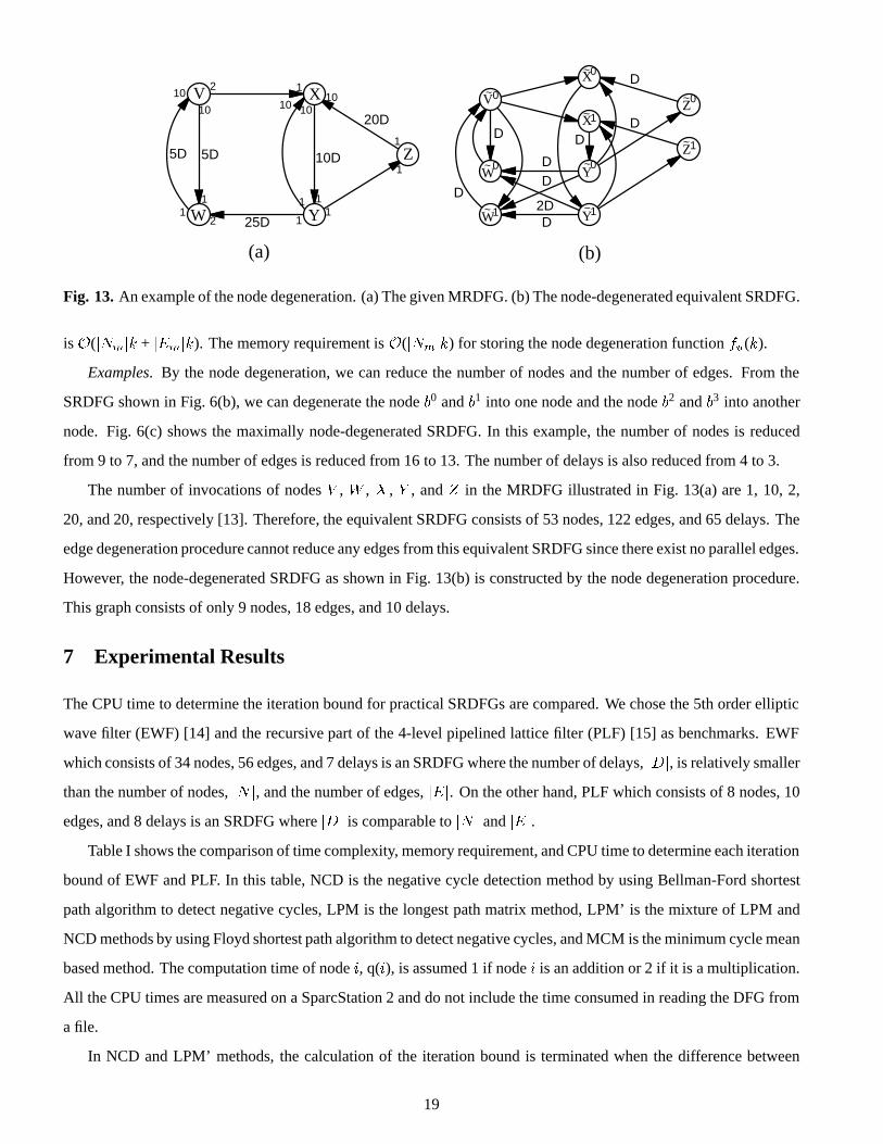
The number of invocations of nodes V , W , X , Y , and Z in the MRDFG illustrated in Fig. 13(a) are 1, 10, 2,

20, and 20, respectively [13]. Therefore, the equivalent SRDFG consists of 53 nodes, 122 edges, and 65 delays. The

edge degeneration procedure cannot reduce any edges from this equivalent SRDFG since there exist no parallel edges.

However, the node-degenerated SRDFG as shown in Fig. 13(b) is constructed by the node degeneration procedure.

This graph consists of only 9 nodes, 18 edges, and 10 delays.

7 Experimental Results

The CPU time to determine the iteration bound for practical SRDFGs are compared. We chose the 5th order elliptic

wave filter (EWF) [14] and the recursive part of the 4-level pipelined lattice filter (PLF) [15] as benchmarks. EWF

which consists of 34 nodes, 56 edges, and 7 delays is an SRDFG where the number of delays, jDj, is relatively smaller

than the number of nodes, jN j, and the number of edges, jEj. On the other hand, PLF which consists of 8 nodes, 10

edges, and 8 delays is an SRDFG where jDj is comparable to jN j and jEj.

Table I shows the comparison of time complexity, memory requirement, and CPU time to determine each iteration

bound of EWF and PLF. In this table, NCD is the negative cycle detection method by using Bellman-Ford shortest

path algorithm to detect negative cycles, LPM is the longest path matrix method, LPM’ is the mixture of LPM and

NCD methods by using Floyd shortest path algorithm to detect negative cycles, and MCM is the minimum cycle mean

based method. The computation time of node i, q(i), is assumed 1 if node i is an addition or 2 if it is a multiplication.

All the CPU times are measured on a SparcStation 2 and do not include the time consumed in reading the DFG from

a file.

In NCD and LPM’ methods, the calculation of the iteration bound is terminated when the difference between

19

Table I Comparison of Iteration Bound Determination Algorithms

CPU [mS]Method Time complexity Memory requirement EWF PLFNCD O(jN jjEj log jN j) O(jN j + jEj) 25.2a 1.00c

LPM O(jDjjEj + jDj

4) O(jN j + jDj

2) 1.92b 2.97d

LPM’ O(jDjjEj + jDj

3 log jDj) O(jN j + jDj

2) 3.58a 6.38c

MCM O(jDjjEj + jDjjE

d

j) O(jN j + jDj

2) 0.717b 0.650dathe obtained iteration bound = 16.0002594 cthe obtained iteration bound = 1.50439453bthe obtained iteration bound = 16.0000000 dthe obtained iteration bound = 1.50000000

Table II Iteration Bound Determination of DFG in Fig. 13

CPU [mS]Method equivalent node-degen.NCD 52.7a 1.45c

LPM 4350b 3.02b

LPM’ 442a 4.10c

MCM 40.7b 0.767bathe obtained iteration bound = 4.0003128 cthe obtained iteration bound = 3.9902344bthe obtained iteration bound = 4.0000000

successive guess iteration bounds becomes smaller than 1=jN j

2

2 where jN j is the number of nodes in the DFG and

is the longest computation time of nodes [6]. While LPM and MCM derive the exact iteration bound, NCD and

LPM’ derive only an approximate iteration bound. Some post-calculations may be necessary to identify the exact

iteration bound from the approximate.

Table II shows CPU times to determine the iteration bounds of the equivalent and node-degenerated SRDFGs of the

MRDFG in Fig. 13(a). All the computation time of nodes are assumed to be 1. We can see that the node degeneration

greatly improves CPU time in any iteration bound methods and that our proposed iteration bound determination

method is the fastest.

8 Conclusions

In this paper we proposed a new method to determine the iteration bound of SRDFGs. Its time complexity is better

than the previously reported methods in the case where the number of delays is relatively smaller than the number of

nodes in the SRDFG. If the number of delays is much larger than the number of nodes, then the NCD method would

be the fastest; however, most digital signal processing algorithms do not fall into this category.

The node degeneration technique to reduce the number of nodes and the number of edges of the equivalent SRDFG

of a MRDFG is also proposed. In some cases, node degeneration may not be applicable. However, if the node-

degeneration is applicable, then it is shown that the iteration bound of the node-degenerated SRDFG can be computed

faster than the approach where either only edge degeneration or no degeneration is applied.

20

In rate-optimal scheduling, the iteration bound is computed many times. Therefore, the node degeneration tech-

nique would play an important role in speeding up the scheduling by minimizing the iteration bound determination

time. In the case of further combining the node degeneration technique into scheduling, careful attention should be

paid since some nodes may have been removed from the node-degenerated SRDFG and operations of those nodes

have to be scheduled as well as the nodes in the node-degenerated SRSFG.

References

[1] K. K. Parhi, “Algorithm Transformation Techniques for Concurrent Processors,” Proc. of the IEEE, vol. 77,pp. 1879–1895, Dec. 1989.

[2] E. A. Lee and D. G. Messerschmitt, “Static Scheduling of Synchronous Data Flow Program for Digital SignalProcessing,” IEEE Trans. Computers, vol. C-36, pp. 24–35, Jan. 1987.

[3] M. Renfors and Y. Neuvo, “The Maximum Sampling Rate of Digital Filters under Speed Constraints,” IEEETrans. Circuits Syst., vol. CAS-28, pp. 196–202, Mar. 1981.

[4] D. A. Schwartz and T. P. Barnwell, III, “A Graph Theoretic Technique for the Generation of Systolic Implemen-tations for Shift Invariant Flow Graphs,” in Proc. of the 1984 IEEE ICASSP, San Diego, CA, Mar. 1984.

[5] K. K. Parhi and D. G. Messerschmitt, “Static Rate-Optimal Scheduling of Iterative Data-Flow Programs viaOptimum Unfolding,” IEEE Trans. Computers, vol. C-40, pp. 178–195, Feb. 1991.

[6] D. Y. Chao and D. Y. Wang, “Iteration Bounds of Single-Rate Data Flow Graphs for Concurrent Processing,”IEEE Trans. Circuits Syst.-I, vol. CAS-40, pp. 629–634, Sept. 1993.

[7] S. H. Gerez, S. M. Heemstra de Groot, and O. E. Herrmann, “A Polynomial-Time Algorithm for the Computa-tion of the Iteration-Period Bound in Recursive Data-Flow Graphs,” IEEE Trans. Circuits Syst.-I, vol. CAS-39,pp. 49–52, Jan. 1992.

[8] K. Ito and K. K. Parhi, “Determining the Iteration Bounds of Single-Rate and Multi-Rate Data-Flow Graphs,” inProc. of 1994 IEEE Asia-Pacific Conf. on Circuits and Systems, Taipei, Taiwan, pp. 6A.1.1–6A.1.6, Dec. 1994.

[9] R. M. Karp, “A Characterization of the Minimum Cycle Mean in a Digraph,” Discrete Mathematics, vol. 23,pp. 309–311, 1978.

[10] R. Govindarajan and G. R. Gao, “A Novel Framework for Multi-Rate Scheduling in DSP Applications,” in Proc.1993 Int. Conf. Application-Specific Array Processors, pp. 77–88, IEEE Computer Society Press, 1993.

[11] E. M. Reingold, J. Nievergelt, and N. Deo, Combinatorial Algorithms: Theory and Practice. Englewood Cliffs,NJ: Prentice Hall, 1977.

[12] E. L. Lawler, Combinatorial Optimization: Networks and Matroids. New York: Holt, Rinehart and Winston,1976.

[13] S. S. Bhattacharyya, J. T. Buck, S. Ha, and E. A. Lee, “A Scheduling Framework for Minimizing MemoryRequirements of Multirate DSP Systems Represented as Dataflow Graphs,” in VLSI Signal Processing, VI,pp. 188–196, 1993.

[14] S. Y. Kung, H. J. Whitehouse, and T. Kailath, VLSI and Modern Signal Processing. Englewood Cliffs, NJ:Prentice Hall, 1985.

[15] J.-G. Chung and K. K. Parhi, “Pipelining of Lattice IIR Digital Filters,” IEEE Trans. Signal Processing, vol. SP-42, pp. 751–761, Apr. 1994.

21