2018 IEEE International Conference on Bioinformatics and Biomedicine (BIBM)

978-1-5386-5488-0/18/$31.00 ©2018 IEEE 283

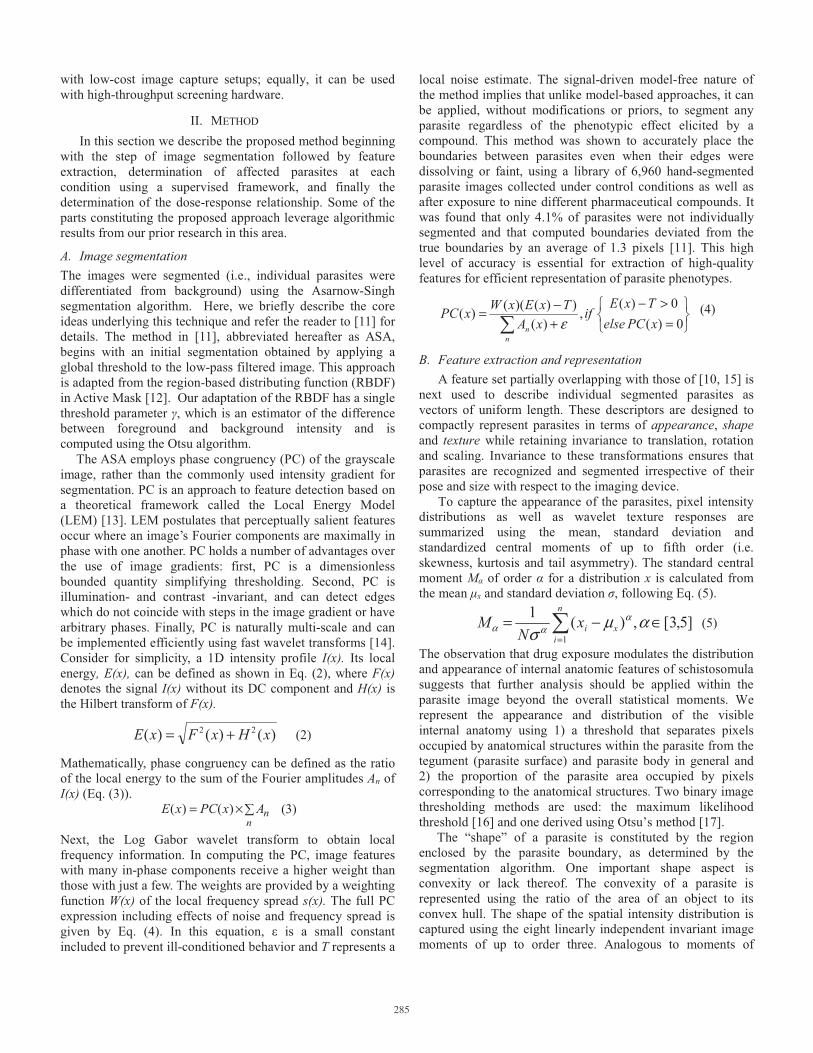
Determining Dose-Response Characteristics of Molecular Perturbations in Whole-Organism Assays

Using Biological Imaging and Machine Learning Daniel Asarnow1,† and Rahul Singh1,2,†

1Department of Computer Science, San Francisco State University, and 2Center for Discovery and Innovation in Parasitic Diseases, University of California, San Diego

Abstract—Advances in microscopy and high-content imaging

now offer a powerful way to profile the phenotypic response of intact systems to molecular perturbation and study the response irrespective of putative target activity and by preserving the physiological context in the living systems. An emerging challenge in bioinformatics and drug discovery is constituted by data generated from such studies that involve analyzing the effect of specific molecules at the system-wide organism level. In this paper we propose a novel automated approach that combines techniques from biological imaging and machine learning to automatically quantify a fundamental measure of molecular perturbation in an intact biological system, namely, its dose-response characteristics. We validate our results using phenotypic assay data involving post-infective larvae (schistosomula) of the parasitic Schistosoma mansoni flatworm. This parasite is one of the etiological agents of schistosomiasis – a significant neglected tropical disease, which puts at-risk nearly two billion people.

Keywords—Whole organism studies, structure-phenotype data, dose-response relationship, phenotypic assays, biological imaging, machine learning.

I. INTRODUCTION One of the fundamental notions in biology and drug

discovery is that of structure-activity relationship (SAR). In a SAR, a property �i induced by a molecule Mi in a biological system S is envisaged as a function of the “chemical constitution” of Mi subject to the specificities of S:

�i = f(Mi) (1) Thus, given a system S, the basic elements needed for establishing a SAR are: (1) a description of the molecular structure and (2) experimental results (called assays) measuring the biochemical property. Consider now the set of molecules M={Mi} and the corresponding biochemical properties �={�i} induced by M in S. M can be thought of as a set of “probes” for investigating S by inducing the characterizing outputs � which vary as elements of M change. In the traditional (reductionist) setting, S tends to be a molecular target and � is limited to a specific bio-chemical response of interest at the molecular level. Target directed formulations have encouraged the application of simplistic enzyme-based or cell-based assays. Though easy to design and run in high-throughput, such assays provide limited information on how complex physiologic systems work and how they may be meaningfully and efficaciously perturbed

(for example to identify potential drugs).† There is ample evidence that target directed drug discovery has led to decline in approval of drugs against new targets and failure of candidate drugs due to lack of systemic efficacy [1-3].

Figure 1. Richness and complexity of structure-phenotype data: (A) Structures of three small molecule probes (from top to bottom): the cysteine protease inhibitor K777, Praziquantel (PZQ), and Niclosamide. (B) phenotypes exhibited by the trematode S. mansoni (from top to bottom): controls, after exposure to K777, and after exposure to PZQ. (C) Results of exposure to Niclosamide shown here as a function of concentration and exposure time. Note the complex phenotypic changes which occur even due to the action of a single compound. These changes have to be modeled precisely and quantitatively to capture the richness in the data.

The alternative lies in measuring and interpreting � at the systems-level by considering the response of cells, tissues, and even entire organisms to the probes. Advances in microscopy and high-content imaging now offer a powerful way to profile the phenotypic response to molecular perturbation and study the response irrespective of putative target activity and by preserving the physiological context in intact living systems. Recent studies have shown the value of such an approach to confirm activity and elucidate detailed molecular mechanisms of action (MOA) [4-6]. In Fig. 1, we present examples of structure-phenotype data from exposure of the trematode S. mansoni (one of the causative agents of the disease schistosomiasis) to three different chemical probes. The reader may observe the systemic effects introduced by these probes in terms of phenotypic changes in shape and appearance

† Equal contributors. DA is currently at the University of California, San Francisco.

284

(changes in terms of motion and behavior also occur). In Fig. 1(c), we also show how the phenotypic effects vary based on the time and concentration of exposure to the compound Niclosamide. A dose-response relationship describes the changes occurring in the organism as the dose (concentration) of the molecular perturbation or the duration of the exposure is varied. Typically, such relationships are expressed as a curve, defining a one-to-one mapping of the system response to changes in concentration or duration of the perturbation. Determining dose-response characteristics is central, among others, to determining the biochemical response-range of a biological system, characterize the phenotypes it exhibits, determine the efficacy of a drug through the calculation of statistics like IC50 (half maximal inhibitory concentration) EC50 (Half maximal effective concentration) or LD50 (median lethal dose), and for determining safe dosage.

A. Problem formulation and technical challenges Given the response of an intact biological system (such as the S. mansoni parasite(s)) either to changes in concentration or exposure time of a molecular perturbation, as shown, for instance, in Fig. 1(c), the problem involves determining a quantitative mapping between the independent variable, i.e. changes in the perturbation and the multidimensional response (phenotypes) exhibited as a consequence by the biological system. Solving this problem requires addressing a number of independent technical challenges, which we summarize below. Hereafter, without loss of generality, we shall assume phenotypic assays conducted on schistosomula to substantiate the problem context. • Segmentation of individual parasites and tracking

individuals across time: Analyzing the effect of drugs on individual schistosomula requires that they be recognized and localized within well micrographs containing tens to hundreds of parasites. Further, given a sequence of images corresponding to observations over time, a correspondence needs to be established for each individual being monitored, so that effects of a drug can be measured longitudinally.

• Definition and accurate measurements of salient phenotypic features (descriptors): Given accurate segmentation and tracking of schistosomula, specific attributes capable of effectively representing the elicited phenotypes must be defined and then measured over an entire population of parasites. Examples of such descriptors can include measurements of the parasite shape and geometry, parasite appearance (such as color and texture), and parasite motion.

• Methodology for mapping the multidimensional system response to low dimensional indicator variable(s): To determine dose-response characteristics, the (multidimensional) dependent variables defined by the phenotype descriptors have to be mapped to a one dimensional indicator variable so that the dose-response relationship can be elucidated.

B. Overview of the proposed approach We utilize the number of parasites differing significantly from controls at specific experimental conditions (e.g. compound and concentration) to compute a quantal-statistic which is subsequently used to determine the corresponding quantitative dose-response characteristics of the parasite population. The determination as to which specific parasites differ significantly from the control is done automatically using a combination of biological imaging and supervised machine learning. The approach begins by representing individual parasites through numerical vectors in a measurement or feature space. These features capture the appearance and geometry of the parasites via image analysis of bright-field micrographs. Next, using a supervised formulation a classifier is trained and subsequently used to determine affected parasites. The classifier is designed using a soft-margin support vector machine employing the Gaussian radial basis function kernel, which is applied in a two-step procedure: first, an average representation of the control population is constructed. Next, this representation is used in conjunction with parasite feature vectors to classify individual schistosomula. The number of affected parasites constitutes the quantal-statistic which is used to obtain the dose-response relationship.

C. Prior work and contributions of the proposed research To the best of our knowledge, at the state-of-the-art, the problem of automatically determining dose-response characteristics from multidimensional measurements of the biological system remains unsolved. A number of methods exist which can map specific phenotypes to variations in chemical perturbations. For example, a whole-organism assay based on electrode measurements of motility has been proposed and applied to multiple experimental conditions [7]. However, only a single schistosome was analyzed. Furthermore, the reliance on a single phenotypic measurement (motility) concomitantly limited the range of drug effects which could be detected. Other specialized measurement assays have taken advantage of the differential uptake of dye compounds by living and dead schistosomula [8-9], to record dose-response information. Unfortunately, this approach is limited to detection of a single, highly specific (albeit interesting) phenotype, namely, parasite death. Other methods (e.g. [10]) have described label free, image-based characterization of phenotypes; however, the problem of determining dose-response characteristics was not attempted.

The proposed approach allows for rigorous and quantitative determination of dose-response characteristics for macroparasites exhibiting complex phenotypic response in whole-organism assays and represents the first known solution to this problem. Owing to the use of a supervised machine learning formulation, our method can incorporate domain expertize in assessing the phenotypic response of parasite populations to drug exposure or other experimental conditions. Finally, the method does not require expensive hardware platforms and can be used to analyze data obtained

285

with low-cost image capture setups; equally, it can be used with high-throughput screening hardware.

II. METHOD In this section we describe the proposed method beginning

with the step of image segmentation followed by feature extraction, determination of affected parasites at each condition using a supervised framework, and finally the determination of the dose-response relationship. Some of the parts constituting the proposed approach leverage algorithmic results from our prior research in this area.

A. Image segmentation The images were segmented (i.e., individual parasites were differentiated from background) using the Asarnow-Singh segmentation algorithm. Here, we briefly describe the core ideas underlying this technique and refer the reader to [11] for details. The method in [11], abbreviated hereafter as ASA, begins with an initial segmentation obtained by applying a global threshold to the low-pass filtered image. This approach is adapted from the region-based distributing function (RBDF) in Active Mask [12]. Our adaptation of the RBDF has a single threshold parameter �, which is an estimator of the difference between foreground and background intensity and is computed using the Otsu algorithm.

The ASA employs phase congruency (PC) of the grayscale image, rather than the commonly used intensity gradient for segmentation. PC is an approach to feature detection based on a theoretical framework called the Local Energy Model (LEM) [13]. LEM postulates that perceptually salient features occur where an image’s Fourier components are maximally in phase with one another. PC holds a number of advantages over the use of image gradients: first, PC is a dimensionless bounded quantity simplifying thresholding. Second, PC is illumination- and contrast -invariant, and can detect edges which do not coincide with steps in the image gradient or have arbitrary phases. Finally, PC is naturally multi-scale and can be implemented efficiently using fast wavelet transforms [14]. Consider for simplicity, a 1D intensity profile I(x). Its local energy, E(x), can be defined as shown in Eq. (2), where F(x) denotes the signal I(x) without its DC component and H(x) is the Hilbert transform of F(x).

)()()( 22 xHxFxE += (2)

Mathematically, phase congruency can be defined as the ratio of the local energy to the sum of the Fourier amplitudes An of I(x) (Eq. (3)).

�×=n

nAxPCxE )()( (3) Next, the Log Gabor wavelet transform to obtain local frequency information. In computing the PC, image features with many in-phase components receive a higher weight than those with just a few. The weights are provided by a weighting function W(x) of the local frequency spread s(x). The full PC expression including effects of noise and frequency spread is given by Eq. (4). In this equation, � is a small constant included to prevent ill-conditioned behavior and T represents a

local noise estimate. The signal-driven model-free nature of the method implies that unlike model-based approaches, it can be applied, without modifications or priors, to segment any parasite regardless of the phenotypic effect elicited by a compound. This method was shown to accurately place the boundaries between parasites even when their edges were dissolving or faint, using a library of 6,960 hand-segmented parasite images collected under control conditions as well as after exposure to nine different pharmaceutical compounds. It was found that only 4.1% of parasites were not individually segmented and that computed boundaries deviated from the true boundaries by an average of 1.3 pixels [11]. This high level of accuracy is essential for extraction of high-quality features for efficient representation of parasite phenotypes.

���

���

=>−

+−=

� 0)(0)(

,)(

))()(()(xPCelse

TxEif

xATxExWxPC

nn ε

(4)

B. Feature extraction and representation A feature set partially overlapping with those of [10, 15] is

next used to describe individual segmented parasites as vectors of uniform length. These descriptors are designed to compactly represent parasites in terms of appearance, shape and texture while retaining invariance to translation, rotation and scaling. Invariance to these transformations ensures that parasites are recognized and segmented irrespective of their pose and size with respect to the imaging device.

To capture the appearance of the parasites, pixel intensity distributions as well as wavelet texture responses are summarized using the mean, standard deviation and standardized central moments of up to fifth order (i.e. skewness, kurtosis and tail asymmetry). The standard central moment M� of order � for a distribution x is calculated from the mean �x and standard deviation �, following Eq. (5).

�=

∈−=n

ixix

NM

1]5,3[,)(1 αμ

σα

αα (5)

The observation that drug exposure modulates the distribution and appearance of internal anatomic features of schistosomula suggests that further analysis should be applied within the parasite image beyond the overall statistical moments. We represent the appearance and distribution of the visible internal anatomy using 1) a threshold that separates pixels occupied by anatomical structures within the parasite from the tegument (parasite surface) and parasite body in general and 2) the proportion of the parasite area occupied by pixels corresponding to the anatomical structures. Two binary image thresholding methods are used: the maximum likelihood threshold [16] and one derived using Otsu’s method [17].

The “shape” of a parasite is constituted by the region enclosed by the parasite boundary, as determined by the segmentation algorithm. One important shape aspect is convexity or lack thereof. The convexity of a parasite is represented using the ratio of the area of an object to its convex hull. The shape of the spatial intensity distribution is captured using the eight linearly independent invariant image moments of up to order three. Analogous to moments of

286

inertia, but with gray-level intensity taking the place of mass, these moments provide a description of the spatial distribution of image intensities which is invariant to translation, rotation and scaling.

We employ two methods for extraction and representation of texture, one based on gray-level co-occurrence matrices and the other using wavelet transforms. Given an image, its gray-level co-occurrence matrices (GLCM) hold the joint probability for a given pair of gray-levels to be separated by a particular displacement vector [18]. Texture is then represented via measurements of the statistical properties of the GLCM (contrast, correlation, energy, entropy, homogeneity). A limitation of the GLCM is the need for a single displacement vector. This need creates a scale dependency, through the displacement distance, as well as a rotational dependency, through the displacement angle. Scale effects are treated by computing the GLCM using five displacement scales (3, 7, 15, 29 and 59 pixels). Rotational invariance within an individual scale is obtained by rotating the displacement vector through four equally spaced orientations and summing the resultant GLCM. We calculate the raw entropy of the image itself in addition to that of the GLCM.

Wavelet analysis decomposes a signal into a basis composed of re-scaled copies of a single “mother” wavelet, in a manner analogous to Fourier analysis (which decomposes the signal into a basis of periodic exponentials). Wavelet analysis has numerous applications in computer vision, including the extraction of perceptual features such as edges and lines, and wavelet response statistics have been found to be an effective, low-dimensional representation of visual texture. Previous work using wavelet texture analysis for high-throughput screening has employed as a basis either the Daubechies or Gabor wavelet families [19]. However, we employ the same log-Gabor wavelets used for phase congruency calculations made during the image segmentation process (see [11]). Such filters have several advantages vis-à-vis the Daubechies and standard Gabor filters, including zero mean at arbitrary bandwidth and strong empirical correspondences with both the amplitude spectra of natural images as well as the spatial frequency responses of neurons in the mammalian visual cortex. More importantly, log-Gabor filters can be shown to maximally localize frequency and phase information, essential for local analysis within images. A rotationally invariant representation of texture at multiple scales is obtained by taking the statistical moments of the maximum response across six equally spaced filter orientations, independently evaluated at each of five scales with center frequencies roughly corresponding to the displacement vector magnitudes used for GLCM construction. The formulation is based on that of [14]. Briefly, the log-Gabor filter with center frequency �0 is constructed in frequency space following Eq. (6). The scale progression is devised such that the ratio �/�0 remains constant, which ensures all individual filters are members of the same wavelet basis (mother wavelet).

���

� −

=2

0

20

)/ln(2)/ln(

)( ωκωω

ω eG (6) A bank of two-dimensional filters with six evenly spaced

orientations are generated by multiplying the filter described in Eq. (6) with an anisotropic spreading function () (we employ a cosine). The filter responses of a parasite image F are then computed according to Eq. (7), where ⊗ denotes the convolution operator.

))()((maxarg θωθ

Γ⊗GF (7)

The texture features at a single scale are finally defined as the statistical moments of the filter responses in the same manner as is done for the raw pixel intensities – i.e. by computing mean, variance and applying Eq. (5). This process is repeated for the five scales leading to 25 wavelet texture dimensions. These descriptor measurements lead to a feature space composed of 71 separate dimensions.

C. Supervised formulation for determining affected parasites Automated phenotype classification based on the parasite feature vectors is undertaken using a supervised learning approach. In supervised learning, training examples, derived for example from annotation by one or more human experts, are used to prepare a learning device, such as a linear regression or neural network. “Learning” differs from “approximation” in that the goal of learning is not merely to memorize the data at hand, but to produce results which generalize to new, heretofore unseen data points. However, the accuracy (closeness to true values) of predictions can only be determined if true values are known. Supervised learning therefore employs a partitioning of an entire data set in which manual annotations are split into training and test groups (as is described for our data set in the Methods). A given learning algorithm will then attempt to obtain a relation between inputs and training data which generalizes to new inputs that the algorithm has not yet been shown. The support vector machine (SVM) is such a supervised learning algorithm which performs binary classification by determining the separating hyperplane with the maximum margin (distance between the hyperplane and the nearest points) in the space of the data [20]. The SVM method has several major advantages. The optimization problem is provably convex, thus a global optimum solution can be found. The SVM also does not require that input dimensions be decorrelated or orthogonalized in any way, and can be applied to nonlinear problems by replacing the Euclidean dot product with any type of nonlinear inner product, called the kernel. Due to low computational complexity, the algorithm is fast in practice, even for high dimensional spaces such as the 71 dimensional feature space used in this work.

In seeking to classify parasite drug responses, the natural phenotypic variations between different parasite subpopulations must be taken into account. Such variations may imbue each set of experiments with a different baseline control response. This fact is reflected in that experts consistently take phenotypic responses of controls into account during manual parasite classification. It also explains

287

our observation that while SVM classification works well for feature vectors which fall far from the decision surface – that is, parasites which are either highly degenerate or completely normal – the classification accuracy tends to be lower for intermediate parasites lying near the boundary. A visual representation of the variability between different subpopulations of schistosomula can be obtained from the features of the normal control parasites projected into the space spanned by their first two principal components (PC). Although these components account for only about 20% of the total variance found in the data, they are sufficient for visualizing the variations between different control groups. Such a two dimensional approximation based on principal component analysis (PCA) is shown in Figure 2. For control parasites, each group is labeled with a distinct color and the group centroids are displayed as large dots. From the figure, it is clear that there is significant variation between these control populations, and it is assumed that this also is the case for the experimental data corresponding to these controls.

Figure 2. Depiction of the variability between populations of schistosomula considered in this work. The feature space representation of 10,578 parasites from the data are projected into a 2D coordinate plane using principal component analysis (PCA). Normal parasites are represented by circles, while degenerate parasites are shown as open triangles. Each separate control group is shown labeled by a unique color (open circles represent non-control normal parasites), and the centroid of each group is displayed as a large, solid dot. The solid line indicates the SVM classification boundary obtained using the proposed method based on the first two principal components. The figure depicts the variability observed between control populations, as well as an approximation of the feature space and decision boundary used for classification.

In order to account for variation between populations within the framework of the SVM classifier, the SVM input vectors are formed by concatenating the raw feature vectors

for a parasite subpopulation to the centroid of the control parasites for that subpopulation which can be considered to be normal (henceforth called the normal control parasites). This allows the distance between parasites to be determined by their control centroids in concert with the parasite features themselves. Doing so requires that the normal control parasites be known, so that their centroids may be computed without spurious perturbations arising from the inclusion of any degenerate parasites present in the control images. However, which of the control parasites are in fact normal will in general not be known.

We resolve this issue by performing the entire classification process in two sequential steps. In the first step, raw feature vectors from the training data are used to train a SVM classifier, which is used in turn to obtain the centroids of the predicted normal control parasites. In the second step, a new classifier is trained using tuples containing the features of both an observation itself and the coordinates of the corresponding control centroid in the feature space. The two-stage procedure can be seen as conceptually akin to the thought process of a human expert, who first observes a control image (necessarily containing a few degenerate parasites) to construct a mental baseline before making decisions pertaining to images of drug-exposed parasites.

Aside from the addition of estimated control centroids to the input vectors, both stages employ the same classification framework. We make use of the soft-margin SVM [21] and a radial basis function (RBF) kernel [22], in conjunction with the sequential minimal optimization algorithm [23], in order to determine the maximum-margin classification surface separating normal and degenerate schistosomula in the descriptor space enumerated above. The feature dimensions are placed on the same scale – a necessary preprocessing step with SVM – by standardizing the distributions along the dimensions to zero mean and unit standard deviation. A set of SVM are then trained, using 10-fold cross-validation to ensure generalization throughout training. The key parameters, namely the scale of the Gaussian RBF � and the magnitude of the soft-margin box constraint C, are set by directly minimizing the cross-validation error using the method of direct search [24-25]. Using this approach, final parameter values obtained by us were � = 6.9 and C = 3.28. For prediction, the set of 10 SVMs constructed during the cross-validated training are applied, and a final classification is obtained by using majority voting between the classifiers. In the following we refer to these SVMs as the SVM bank. Data sampling conducted during cross-validation is stratified such that the relative distributions of “normal” and “degenerate” parasites are preserved. In addition to visualizing the variation between control populations, Figure 2 provides an example of a decision surface found by SVM with RBF kernel (solid black line). This boundary was found using the two-stage classification procedure within the 2D PCA projection. The efficacy of the procedure is clear given the approximate nature of the data, as the normal parasites (open and colored circles) are found almost entirely opposite the classification boundary from the degenerate ones (open triangles).

288

The reader may note that unlike the one-way analysis of variance (ANOVA) employed in previous automated assays against schistosomiasis [10], the machine learning-based approach as described above does not rely on several key assumptions about the statistics of the data. Namely, these are the assumptions that the response variables are independent and normally distributed, that the population variances are equal, and finally that group responses are independent and identically distributed random variables. None of these assumptions might be expected to hold for the wide variety of complex, image-based measurements used to build the parasite feature space. Furthermore, ANOVA in general loses efficacy when presented with unbalanced data in which different treatment classes are over or under-represented [26]. This is especially troublesome for drug screening, where certain drugs are likely to be studied in much greater than detail than others, which are of less therapeutic interest. The approach to image-based classification of schistosomula developed above does not make any of the listed assumptions and is robust to unbalanced data so long as sufficient sampling of control parasites is made.

D. Determination of dose-response characteristics and EC50 values

Identification and counting of normal and degenerate parasites is performed computationally after segmentation, feature extraction and classification using the previously trained set of SVMs. Following the standard convention, at a given point in time, the drug response is defined as the proportion of degenerate parasites in the well. With n multiple replicate experiments each containing Di degenerate parasites and Ni parasites in total, the empirical response R is computed as shown in Eq. (8).

�=

=n

i i

i

NDR

1

(8)

This definition describes the quantal response (in population weighted average across experiments), which is commonly used when a binary phenotypic effect is observed (such as that between normal and degenerate schistosomula). In addition to the mean, the standard deviation is also calculated.

The (quantal) EC50 is calculated by fitting of the Hill Equation to dose-response data. We use the model specified by Eq. (9), where Rmin and Rmax are the minimum and maximum response values, respectively, m is the Hill coefficient and x is the concentration.

m

ECx

RRRR −

���

�+

−+=

50

minmaxmin

1

(9)

The regression is computed using the trust-region-

reflective nonlinear least-squares algorithm [27], with m constrained to equal 1, and Rmin and Rmax constrained to the interval [0,1]. The constraints on response values are needed to avoid unphysical proportions of parasites, while the fixed value of m forces the model to represent a noncooperative

ligand binding process. Analogous responses are also calculated using the training annotations, rather than the parasite feature vectors in the test data. These results represent the output of the manual version of the assay, and are used for validation of the response curves produced by the assay. Note again that in contrast to other methods the proposed approach has only modest software and hardware requirements which can easily be met using inexpensive, commodity products.

III. EXPERIMENTS, EVALUATIONS AND RESULTS

A. Experiment design We prepare the machinery of the method (i.e. a set of non-linear SVMs) using the 4,256 parasites in the designated training data, and the single training vector obtained by majority voting between the experts. Assay performance is quantitated in two stages. First, confusion analysis is applied directly to the classification of the testing data obtaining using the SVM bank. The confusion analysis is performed using the manual annotations of the test parasites. It is important to note here that these annotations were not used in any manner whatsoever during training. Second, dose-response curves generated using the SVM classifications are compared to those obtained from the manual annotations. This comparison reflects the accuracy of the automated assay in replicating the manual assay performed by human experts.

B. Measures for analyzing classification performance The classification performance was evaluated by comparing the results of automatic classification to a ground truth (here, manual annotations obtained from domain experts). The analysis consists in computing the number of true positives TP, false positives FP, true negatives TN and false negatives FN, as well as several derived statistics, taking normal parasite classifications to be “negative,” and degenerate ones to be “positive.” The derived statistics included the true negative and true positive rates TNR and TPR, the negative and positive predictive values NPV and PPV, and the accuracy ACC. In addition, we calculated two additional measures, the Matthew’s correlation coefficient MCC, a descriptor of overall classification performance which is robust to unbalanced class sizes, and the F1-measure, which is the harmonic mean of precision (PPV) and recall (TPR).

C. Classification performance on the test set In Figure 3, we present the confusion matrix for the test set. In this case, classification was performed with the dual-layer method. The matrix presents assessments of the classification in terms of the aforementioned TP, FP, TN and FN measures, both in terms of the numbers of parasites and as percentages. Figure 3 also shows FPR, TPR, NPV, PPV and ACC adjacent to the row or column of the confusion matrix from which they are computed (ACC is computed from the diagonal). The matrix indicates that 58.5% of the test parasites are correctly classified as normal and 32.1% as degenerate, while just 5.0% and 4.4% of parasites are incorrectly classified as normal or degenerate, respectively. The overall classification accuracy is thus 90.6%, while the MCC and F1-measure are also quite

289

high, at MCC=0.798 and F1=0.872, respectively. These results clearly demonstrate the efficacy of the outlined procedure for automatic classification of “normal” and “degenerate” parasites based on classification boundary learnt from the human experts.

Figure 3. Confusion matrix for classification of the test set. The matrix shows the proportion of correctly and misclassified cases of each type (TN, FN, FP and TP), and additionally shows five statistical measures of classification quality, namely accuracy, TPR (recall), TNR, PPV (precision) and NPV. Each of these statistics is shown adjacent to the row or column of the confusion matrix from which it is calculated. Raw values are shown in green, and are subtracted from 1 and shown in red for ease of comparison. In addition to the measures shown above, the Matthew’s correlation coefficient for this confusion matrix is 0.798, and the F1-measure is 0.872.

D. Dose-response characterization of drugs The dose-response characteristics of the investigated compounds as determined using the proposed method for twelve distinct compounds is shown in Figure 4. As mentioned earlier, “consensus” training data can be obtained using majority voting. The use of such data with the SVM bank classifier proposed here constitutes an elegant means for arriving at a single set of dose-response curves as the output of the automated assay. The dose-response curves obtained using majority voting across the human experts are depicted in this figure. It can be seen here that there is a close correspondence between the dose-responses curves derived from the manual screen and those obtained using the fully automated approach described above. Pearson’s correlation coefficients between these curves, as well as the corresponding p-values, are listed in Table 3. The p-values are estimated using Student’s t-distribution under the alternative hypothesis that the correlation is not zero. The correlations are � 0.93 and are highly significant (p-value � 0.05) for all compounds, including the two (rosuvastatin and sorafenib) which were novel to the method. The minimum correlation is observed for the drug praziquantel, for which the automated assay deviates from the manual at high concentrations. This discrepancy was primarily due to the disagreement in the assessments of the individual experts in analyzing the impact of this compound in terms of impact on parasites.

Table 3. Dose-response correlations between manual and automated assay. Pearson’s product-moment correlation coefficients and p-values computed with Student’s t-test are listed for each compound. Reported values are derived using the test data set.

Compound Correlation p-value Atorvastatin 0.996 4.00 * 10-3 Fluvastatin 0.985 1.50 * 10-2 Lovastatin 0.989 1.12 * 10-2 Pravastatin 0.956 4.24 * 10-2 Simvastatin 0.992 9.02 * 10-4 Closantel 0.993 7.98 * 10-6 Ibandronate 0.993 7.25 * 10-4 K11777 0.964 8.00 * 10-3 Niclosamide 0.996 3.47 * 10-4 Praziquantel 0.932 2.13 * 10-2 Rosuvastatin 0.995 5.20 * 10-3 Sorafenib 0.998 4.99 * 10-7

290

V. Conclusions In this paper we have described the design, implementation and assessment of a fully automatic, quantitative approach for dose-response characterization in whole-organism assays using biological imaging and machine learning. To the best of our knowledge, this is the first known solution to this problem. The bioimage analysis of our method segments multiple parasites in whole-well images, including touching and partially overlapping somules. A learning model employing non-linear SVM then classifies segmented schistosomula within a high-dimensional feature space, the dimensions of which correspond to measurements of appearance, shape and texture. The model possesses two layers: one in which putatively “normal” parasites are identified within each control image and used to derive an estimated control centroid, and one in which all parasites are classified as “normal” or “degenerate” on the basis of tuples composed of a given parasite’s feature vector and corresponding control centroid. Such a procedure is essential because the variation between different populations of unavoidably create different baselines for different experiments. The learning model was trained on manually annotated images using cross-validation to produce a dual-layer SVM bank; each bank makes individual predictions using majority voting within the bank. The analysis of classification results for the test data confirms the efficacy of the proposed method: it has an overall classification accuracy of 90.5%. Furthermore, the dose-response curves (in terms of the proportion of degenerate parasites) determined using the predicted classifications correlate tightly with those computed from the training data.

VI. Acknowledgements The authors thank Conor R. Caffrey and Liliana Arreola-Rojo for providing the schistosome screening data used in the computational analysis and for providing a manual assessment of the chemical insults undergone by the parasites. This research was funded in part by the National Science Foundation through grant IIS 1817239.

References

[1] F. Sams-Dodd, “Target-based drug discovery: is something wrong?”, Drug Discovery Today, 10 (2005):139-147.

[2] E. C. Butcher, “Can cell systems biology rescue drug discovery?”, Nature Reviews in Drug Discovery, 4 (2005): 461-467.

[3] D. C. Swinney and J. Anthony, “How were new medicines discovered?,” Nature Reviews Drug Discovery, vol. 10, no. 7, (2011) pp. 507–519.

[4] T. Long, et al., “Structure-bioactivity relationship for benzimidazole thiophene inhibitors of polo-like-kinase 1 (PLK1), a potential drug target in Schistosoma mansoni”, PLoS Neglected Tropical Diseases, (2016)10(1):e0004356.

[5] L. R. Areola, et al., “Chemical and Genetic Validation of the Statin Drug Target for Treating the Helminth Disease Schistosomiasis”, PLoS One, 9(1) (2014): e87594.

[6] K. C. Peach et al., “Mechanism of action-based classification of antibiotics using high-content bacterial image analysis”, Molecular Biosystems, 9 (2013): 1837-1848.

[7] Smout MJ, Kotze AC, McCarthy JS, Loukas A (2010) A Novel High Throughput Assay for Anthelmintic Drug Screening and Resistance Diagnosis by Real-Time Monitoring of Parasite Motility. PLoS Negl Trop Dis 4: e885.

[8] Peak E, Chalmers IW, Hoffmann KF (2010) Development and Validation of a Quantitative, High-Throughput, Fluorescent-Based Bioassay to Detect Schistosoma Viability. PLoS Negl Trop Dis 4: e759.

[9] Mansour NR, Bickle QD (2010) Comparison of Microscopy and Alamar Blue Reduction in a Larval Based Assay for Schistosome Drug Screening. PLoS Negl Trop Dis 4: e795.

[10] Paveley RA, Mansour NR, Hallyburton I, Bleicher LS, Benn AE, et al. (2012) Whole Organism High-Content Screening by Label-Free, Image-Based Bayesian Classification for Parasitic Diseases. PLoS Negl Trop Dis 6: e1762.

[11] D. Asarnow, R. Singh, “Segmenting the etiological agent of schistosomiasis for high-content screening”, IEEE Transactions on Medical Imaging, (2013), pp. 1007-1018.

[12] G. Srinivasa, et al., “Active Mask Segmentation of Fluorescence Microscope Images”, IEEE Transaction on Image Processing, vol.18, (2009) pp. 1817-1829.

[13] M.C. Morrone, D.C. Burr, “Feature detection in human vision: a phase-dependent energy model”, Proc. of the Royal Society of London. Series B, Biological sciences, vol. 235, (1988) pp. 221-245.

[14] P. Kovesi, “Image features from phase congruency”, Videre, March 1995

[15] Lee H, et al., “Quantification and clustering of phenotypic screening data using time-series analysis for chemotherapy of schistosomiasis”, BMC Genomics 13: S4 (2012).

[16] Glasbey CA An Analysis of Histogram-Based Thresholding Algorithms. CVGIP Graph Models Image Process 55 (1993) 532–537

[17] Otsu N A Threshold Selection Method from Gray-Level Histograms. IEEE Trans Syst Man Cybern 9: (1979) 62–66.

[18] Haralick RM, Shanmugam K, Dinstein I. “Textural Features for Image Classification”. IEEE Trans Syst Man Cybern 3 (1973): 610–621..

[19] Manjunath BS, Ma WY (1996) Texture features for browsing and retrieval of image data. IEEE Trans Pattern Anal Mach Intell 18: 837–842.https://www.reddit.com/dev/api/

[20] Vapnik VN (2006) Estimation of dependences based on empirical data. New York, N.Y: Springer..

[21] Cortes C, Vapnik V (1995) Support-vector networks. Mach Learn 20: 273–297.

[22] Boser BE, Guyon IM, Vapnik VN (1992) A training algorithm for optimal margin classifiers. Proceedings of the fifth annual workshop on Computational learning theory. COLT ’92. New York, NY, USA: ACM. pp. 144–152

[23] Platt JC (1998) Sequential Minimal Optimization: A Fast Algorithm for Training Support Vector Machines. Advances in Kernel Methods – Support Vector Learning.

[24] Audet C, Dennis JE (2002) Analysis of Generalized Pattern Searches. SIAM J Optim 13: 889–903.

[25] Kolda TG, Lewis RM, Torczon V (2003) Optimization by Direct Search: New Perspectives on Some Classical and Modern Methods. SIAM Rev 45: 385–482.

[26] Montgomery DC (2008) Design and Analysis of Experiments. John Wiley & Sons.

[27] Coleman TF, Li Y (1996) An Interior Trust Region Approach for Nonlinear Minimization Subject to Bounds. SIAM J Optim 6: 418–445.