This journal is c The Royal Society of Chemistry 2010 Chem. Soc. Rev.

Determining association constants from titration experiments in

supramolecular chemistryw

Pall Thordarson*

Received 10th August 2010

DOI: 10.1039/c0cs00062k

The most common approach for quantifying interactions in supramolecular chemistry is a

titration of the guest to solution of the host, noting the changes in some physical property

through NMR, UV-Vis, fluorescence or other techniques. Despite the apparent simplicity of this

approach, there are several issues that need to be carefully addressed to ensure that the final

results are reliable. This includes the use of non-linear rather than linear regression methods,

careful choice of stoichiometric binding model, the choice of method (e.g., NMR vs. UV-Vis) and

concentration of host, the application of advanced data analysis methods such as global analysis

and finally the estimation of uncertainties and confidence intervals for the results obtained.

This tutorial review will give a systematic overview of all these issues—highlighting some of the

key messages herein with simulated data analysis examples.

1. Introduction

The field of modern supramolecular chemistry continues to

grow from strength to strength from its humble beginnings in

1960–1970 with the pioneering work of Pedersen, Lehn and

Cram that was subsequently recognised by the Nobel prize in

1987.1–3 One of the fundamental issues in supramolecular

chemistry has always been the quantitative analysis of the

intermolecular interactions of interest. The most common

approach to address this issue is the supramolecular titration

method. Here, one component (guest) is gradually added to

the system (host) while monitoring a physical property such

as specific chemical resonance (NMR) or absorption band

(UV) that is sensitive to the supramolecular interaction(s) of

interest. The resulting information is then compared and fitted

to binding models to obtain information such as the associa-

tion constant Ka (See Appendix A for abbreviations used in

this tutorial review.), energetics (DG, DH and DS) and stoichio-

metry (1 : 1 vs. 1 : 2 etc).

The very first crown-ether reported by Pedersen was the

dicyclohexyl-18-crown-6 (Fig. 1a, n.b., at the time of this work

the exact stereochemistry of this host was not defined).4

Although a lot of the subsequent work was done with ion-

selective electrodes, the first report on the association constant

for cis-dicyclohexyl-18-crown-6 binding of potassium (K+)

and other alkali metals applied calorimetric titration to obtain

Ka = 100 for K+ (solvent, temperature and counterion were

not specified).5 A recent, much more complex example for

Fig. 1 Typical supramolecular equilibria. (a) Pedersen’s dicyclohexyl-

18-crown-6 (the stereochemistry was not specified) binding to a

potassium ion.4,5 (b) Squaring cooperative cycles with porphyrin clip

host (blue), viologen (red) and tert-butyl pyridine (green).6

School of Chemistry, The University of New South Wales, Sydney,NSW 2052, Australia. E-mail: p.thordarson@unsw.edu.au;Fax: +61 29385 4478; Tel: +61 29385 4478w Electronic supplementary information (ESI) available: Matlab m-filesfor analysing and simulating 1 : 1, 1 : 2 and 2 : 1 equilibria for NMRand UV-Vis titration, including example data files. See DOI: 10.1039/c0cs00062k

Pall Thordarson

Pall Thordarson obtained hisBSc from the University ofIceland in 1996 and a PhDfrom The University ofSydney in 2001, followed bya Marie Curie Fellowship atthe University of Nijmegen,The Netherlands. He returnedto Australia in 2003 andobtained an ARC AustralianResearch Fellow at The Univer-sity of Sydney in 2006. He wasappointed as a Senior Lecturerat the University of New SouthWales (UNSW), Sydney,Australia, in 2007 where he

leads a research group working on light-activated bioconjugatesfor controlling enzyme activity, self-assembled gels for drugdelivery and supramolecular chemistry.

TUTORIAL REVIEW www.rsc.org/csr | Chemical Society Reviews

Dow

nloa

ded

by N

ew Y

ork

Uni

vers

ity o

n 06

Dec

embe

r 20

10Pu

blis

hed

on 0

1 D

ecem

ber

2010

on

http

://pu

bs.r

sc.o

rg |

doi:1

0.10

39/C

0CS0

0062

KView Online

Chem. Soc. Rev. This journal is c The Royal Society of Chemistry 2010

what sort of data can be extracted from relatively simple

titration studies (fluorescence) comes from Rowan and

co-workers in their study on ‘‘squaring cooperative cycles’’

(Fig. 1b).6 The bulk of the current literature employing

supramolecular titration is somewhere between the two above

extremes in terms of simplicity vs. complexity, with the

emphasis shifting towards the latter.

The quality of the information gained from supramolecular

titrations depends on a number of factors. These include of

course operational factors such as purity of compounds used

or accuracy of the measurement devices used. However, the

planning, execution and subsequent data analysis are as

important. Careful consideration of all these factors is the

key to obtaining quality information that can then be used to

guide further research into the application of the systems. The

above mentioned example of squaring cooperative cycles is a

good example—without proper quantitative data, the applica-

tion of cooperative interactions to direct self-assembly7

becomes an empirical rather than predictable science. Many

excellent textbooks and reviews deal with some of these issues,

such as the much quoted monograph by Connors on binding

constants.8 That said, many researchers still get caught in

avoidable traps such as using out-dated linear regression

methods in data analysis or over-reliance on the Job’s method

to determine stoichiometry, to name just two examples of

other important issues in the determination of association

constants from supramolecular titration. This tutorial review

aims to help people avoid these traps and identify the key

issues involved in planning, executing and analysing data

from supramolecular titration experiments. To simplify the

discussion the emphasis will be on relatively simple host–guest

equilibria such as the formation of 1 : 1, 1 : 2 and 2 : 1

complexes but the lessons learned from these systems can also

be applied to more complex systems such as the cooperative

aggregation of monomers into oligomers.9 The review will

start by outlining some of the key dos and don’ts of

supramolecular titrations before moving on to a more detailed

description of equations and equilibria, determination of

stoichiometry, common techniques and data analysis.

2. Dos and don’ts of supramolecular

titration experiments

At the outset of this tutorial review it is useful to list some of

key messages contained herein in the form of fourteen dos and

don’ts:

1. Do try to obtain as much information as possible prior to

carrying out the titration experiment on what the expected

outcomes are. Look at related or similar systems for clues.

Starting with a reasonable estimation of what the stoichiometry

and the association are likely to be will make it easier to choose

the right technique, concentration of host/guest, number of

addition points, etc. If little or no helpful information exists on

the system of interest a quick preliminary titration experiment

might be worthwhile.

2. Don’t just simply apply a ‘‘black box’’ binding model

from a computer program or a book without trying to under-

stand how they are derived from the underlying equilibria.

Understanding the link between binding equilibria and

the equations used to obtain binding constants helps with

evaluating how robust the results are and whether the right

model has been used to analyse the data.

3. Do take the extra time necessary to carry out the actual

titration experiment with as much care as possible. Check the

purity of chemicals used and thoroughly clean any glassware

used. Use the most accurate methods available to measure out

the solution—often weighing out the solvents for solutions

is much more accurate than relying simply on volumetric

glassware. Avoid dilution factors, e.g., by preparing the guest

solutions in the host solution with the same concentration of

the host for the titration. This will ensure the host concentra-

tion stays constant during the course of the experiment

cancelling (mostly) out any additional effects from aggregation

of the host. Make sure to control and record the temperature.

An accurate association constant at an unknown temperature

is of little value.

4. Don’t choose an instrumental method to follow the

course of titration on economical (I don’t need deuterated

solvents for UV-Vis) or emotional (I really like doing NMR)

grounds but try to pick the method that is most applicable to

the system of interest. Admittedly, economical reasons do

sometimes play a role (e.g., access to calorimeters is not

universal) but the primary concern should be factors such as

concentration vs. expected association strength (NMR works

well with Ka o 100 000 M-1), nature of host/guest used

(e.g., chromophores) or the potential influences of impurities

(fluorescence spectroscopy can be more sensitive to impurities

than UV-Vis spectroscopy).

5. Do aim to get a reasonable number of titration points

(additions) as practically feasible in a reasonable short time.

The extra time spent getting a reasonable number will ensure

better certainty in the data fitting process, especially when

strong interactions or more complex equilibria such as 1 : 2

host/guest complexation can play a role. Note that collecting a

large number points can be counterproductive due to building

of systematic errors over time (e.g., evaporation of solvent).

On balance it is better to collect 3 titrations with 15 data points

than one with 45 points.

6. Don’t take any shortcuts in the data analysis, especially

by using out-dated linear regression methods such as the

Benesi–Hildebrand/Lineweaver–Burk, Scott/Hanse–Woolf or

Scatchard transformations. These methods were useful before

modern computers and programs became available but they

introduce a number of errors and problems that can be

avoided with modern computer-based non-linear regression

methods. Related to this is the problem of making assump-

tions such as equating the total concentration of the guest

([G]0) with the free (unbound) concentration of the guest

[G] or that the measured quantity (e.g., absorbance change

DA) equals the change in the concentration of the complex

([HG]). Frequently, these problems can be traced back to

using approaches that still work well in studying association

phenomena in biochemistry but are actually not applicable to

typical supramolecular chemistry titrations. Finally, when

analysing 1 : 2 or more complex equilibria, use programs that

can handle the underlying cubic or more complex equations

rather than making unnecessary and risky shortcuts.

Dow

nloa

ded

by N

ew Y

ork

Uni

vers

ity o

n 06

Dec

embe

r 20

10Pu

blis

hed

on 0

1 D

ecem

ber

2010

on

http

://pu

bs.r

sc.o

rg |

doi:1

0.10

39/C

0CS0

0062

KView Online

This journal is c The Royal Society of Chemistry 2010 Chem. Soc. Rev.

7. Do consider all sensible possible stoichiometries and use

as many techniques as possible to verify or otherwise a

possible stoichiometric model.

8. Don’t rely exclusively on one particular method to

determine stoichiometry such as the Job’s method which really

only works well when there is one type of complex present—

usually the 1 : 1. If possible and at least remotely probable, the

data should be analysed for more than one type of stoichiometry

and the results then evaluated (see Section 4 below).

9. Do consider the method of global analysis or simultaneous

fitting of multiple datasets to a single binding model.

Generally this improves the fitting processes by tightening

the error surfaces and thus increasing the likelihood that the

solution found in the regression process is the true and not a

local minimum.

10. Don’t forget to critically compare different data analysis

(fitting) results in terms of the number of parameters, etc. used.

With a high enough number of parameters, any data can be

fitted accurately. Look also beyond the association constant

obtained; if other parameters obtained are nonsensical, such as

a chemical shift difference of +120 ppm in 1H NMR studies,

the model used is probably invalid. Also, if the fitting results

are ‘‘unstable’’ in terms of sensitivity to the initial guess of

parameters, the results are probably not reliable.

11. Do repeat the titration. A value from a single run titration

should not be published. Repeating titration is invaluable when

it comes to estimating uncertainties.

12. Don’t just accept the output of the data analysis

program; think about the shape and information content of

the binding isotherm and the residual plot.

13. Do try to estimate the uncertainty in your final results.

Estimating confidence intervals based on asymptoting standard

errors does sometimes work but this method needs to be used

with great care as it is based on assumption that strictly don’t

apply to non-linear regression methods. Additionally, this

popular (and other related classical) statistical methods ignore

uncertainties in factors such as the host concentration which

often is the largest one in the system. Other approaches can be

used (e.g., Monte Carlo) but in the end nothing really replaces

repeating the experiment several times to obtain some sort of a

statistically meaningful estimation of uncertainty in the results

obtained.

14. Don’t focus just on the association constants obtained

when interpreting the results and comparing with other

systems. Think also about the results in terms of energy:

DG = �RTln Ka. Doubling an association constant increases

DG by �1.7 kJ mol�1—this equates to 18% increase in

energy in going from Ka of 50 M�1 to 100 M�1 whereas for

Ka = 500 000 M�1, doubling the association constants only

increases the DG by 5%. Additionally, one needs to consider

statistical factors when analysing results from multivalent

interactions, e.g., in the case of 1 : 2 complexation where

K1 = 4K2 if there is no cooperativity in the system.

The above list is not exhaustive but it should help with

ensuring that the final outcomes of a supramolecular titration

experiment are reliable for interpretation. The more detailed

discussion below will expand on these points—comparing

approaches and techniques and highlighting some of the issues

with simulations of typical titration data.

3. Equations and equilibria—quantifying the

extent of complexation

The below discussion is largely based on previous textbooks

and reviews on determining binding constants.8,10,11 To

facilitate better understanding of the remainder of this tutorial

review for newcomers to the field, the derivation of the key

equations is summarised here again, focusing on 1 : 1 equilibria.

A summary of all the key equations for 1 : 1, 1 : 2

and 2 : 1 equilibria is provided in Charts 1–3—this might

also be useful for readers who are quite familiar with these

equations.

3.1 The basics—equilibria and association constants

With the aid of computer programs designed for determining

association constants from titration experiments, one might be

tempted to ignore the underlying equilibria and the associated

mathematical equations, and just report the answers obtained

from these programs. This ‘‘black box’’ approach is, however,

unwise as without this understanding it becomes very difficult

to answer such questions as: (i) did I determine the stoichiometry

correctly, (ii) did I use the right binding model and how I can

compare different models, (iii) did I use the right technique

and concentration(s) of the host/guest used and finally

(iv) how reliable are the results obtained? The first step

toward answering these questions is to look at how the

typical equilibria in supramolecular chemistry is defined,

starting with the simple 1 : 1 equilibria (Fig. 2a) according

to eqn (1).8,10,11

Ka ¼½HG�½H�½G� ð1Þ

The choice of ‘‘host’’ and ‘‘guest’’ is somewhat arbitrary

but in this tutorial review the host concentration is the one that

is kept constant while being titrated with the guest. For

practical reasons, the host is usually the larger, more expensive

(or more synthetically challenging) component in these systems.

It should be pointed out that other textbooks and references

may use the different terms such as ligand, receptor or the

substrate for either (or both) the host or the guest as they have

been defined here. The thermodynamic association constant

Kx is related to kinetics of the particular system, hence

Ka = k1/k�1, with the k1 and k�1 the forward (on) and

backward (off) rate constants for the equilibria of interest. If

these rate constants can be measured, the association constant

Ka can be calculated directly, but these kinetic methods are

outside the scope of this review.

The 1 : 1 equilibria is just a special case of general equation

for the formation of any supramolecular m � host�n � guest

complex (Fig. 2b) according to eqn (2).10

bmn ¼½HmGn�½H�m½G�n ð2Þ

When m = n = 1 we arrive back at eqn (1) while m = 1 and

n= 2 describes the fairly common 1 : 2 equilibria (Fig. 2c) for

two guests bound to a host. It would be extremely unlikely for

such a termolecular complex to form by simultaneous collision

of one host with two guest—a step wise process as described in

Dow

nloa

ded

by N

ew Y

ork

Uni

vers

ity o

n 06

Dec

embe

r 20

10Pu

blis

hed

on 0

1 D

ecem

ber

2010

on

http

://pu

bs.r

sc.o

rg |

doi:1

0.10

39/C

0CS0

0062

KView Online

Chem. Soc. Rev. This journal is c The Royal Society of Chemistry 2010

eqn (3) and (4) is a more plausible description of how such a

complex is formed.10,11

K1 ¼½HG�½H�½G� ð3Þ

K2 ¼½HG2�½H�½HG� ð4Þ

The relationship between these stepwise constants and their

physical meaning will be described in further details below

after methods to determine association constants for 1 : 1

systems have been described.

3.2 The archetypical 1 : 1 system

Exactly how do we quantify [H], [G] and [HG] in eqn (1)? In

biochemistry it is sometimes possible to measure directly the

concentration of the complex [HG] (or [H] or [G]) by methods

such as electrophoresis.12 If the concentration of the complex

[HG] is known the remaining concentrations can be determined

by the mass balance as described by eqn (5) and (6) for simple

1 : 1 binding.

[H]0 = [H] + [HG] (5)

[G]0 = [G] + [HG] (6)

Unfortunately, it is usually not possible to measure [HG]

(or [H] and [G]) in supramolecular chemistry experiments, but

the knowledge of these is required to determine Ka according

to eqn (1). The only notable exception is when the free host

and guest are in true slow exchange with their complexes on

the NMR timescale so that two distinct peaks can be observed.

In this case it is in principle possible to obtain the con-

centration(s) of the species involved by integration but as

discussed below, this approach is confounded by a number

of issues, limiting its appeal even further. Thankfully, there are

other accurate methods available for the determination of

Ka—methods that rely on indirectly determining the concen-

tration of the complex [HG] from titration experiments.

Supramolecular titration experiments are usually carried out

by fixing the concentration of one component, the host (H),

while the concentration of another component, the guest (G),

is varied (this has also been called the dilution method).

During the course of this titration, the physical changes in

the system are monitored, usually spectroscopically, and this

change is then plotted as a function of guest added to host

(equivalent guests). The resulting titration curve known as

a binding isotherm is then fitted to a mathematical model that

is derived from the assumed equilibria to obtain the association

constant (Ka) and/or other physical constants of interest.

The mathematical model used to obtain the association

constant is usually developed from realising that the physical

change (DY, e.g., a NMR shift or an change in UV-Vis

absorbance) observed is correlated to the concentration of

the complex [HG] as DY p [HG], or in some cases, the free

host [H] or the free guest [G]. The physical change (Y) being

monitored can usually be described as the aggregate of the

individual components according to eqn (7) as a function of

concentration (e.g., for UV-Vis spectroscopy) or eqn (8) as a

function of mole fractions fX (fX defined as: fX = [X]/[X]0) in

the special case of NMR.

Y = YH[H] + YG[G] + YHG[HG] (7)

Y = YHfH + YGfG + YHGfHG (8)

The mole fraction notion is particularly helpful as when we

combine it with the mass balance eqn (5) and (6) and the definition

of the association constant in eqn (1), we obtain eqn (9).8,10

fHG ¼Ka½G�

1 þ Ka½G�ð9Þ

This equation describes the general binding isotherm for a

simple 1 : 1 binding system as a hyperbolic (Fig. 2d) relation-

ship between fHG and the free guest ([G]) concentration.

Therefore, if the free guest concentration was known, it should

be quite straightforward to determine the association constant

assuming the observed physical change (DX) is related to the

mole fraction of the complex, as it usually is. Sadly, the free

guest concentration [G] cannot usually be measured directly so

two alternative approaches are required to solve this problem,

both that result in quadratic equations containing only

the total concentrations ([H]0 and [G]0) and the association

constant (Ka) as the unknown:

In the first approach, we start by realising that since

fHG = [HG]/[H]0, eqn (9) can also be written as

[HG] = [H]0Ka[G]/(1 + Ka[G]) which after insertion to

eqn (6) yields [G]0 = [G] + H0Ka[G]/(1 + Ka[G]). Rearranging

yields the quadratic eqn (10) which has only one relevant real

solution according to eqn (11).8,10

G2 � ½G� G0 �H0 �1

Ka

� ��G0

Ka¼ 0 ð10Þ

½G� ¼ 1

2G0 �H0 �

1

Ka

� �

�

ffiffiffiffiffiffiffiffiffiffiffiffiffiffiffiffiffiffiffiffiffiffiffiffiffiffiffiffiffiffiffiffiffiffiffiffiffiffiffiffiffiffiffiffiffiffiffiffiffiffiffiffiffiG0 �H0 �

1

Ka

� �2

þ 4G0

Ka

s ð11Þ

Alternatively, we can rearrange eqn (5) and (6) to isolate for

[H] and [G], respectively, and insert these into eqn (1) to

Fig. 2 (a)–(c) Three of the supramolecular equilibria discussed in this

review: H = host, G = Guest and HxGx = host–guest complex of

interest, Kx = the thermodynamic association constant for a particular

interest and bmn = overall association constant for an m : n host–guest

complex formation. (d) A typical binding isotherm. See text for details.

Dow

nloa

ded

by N

ew Y

ork

Uni

vers

ity o

n 06

Dec

embe

r 20

10Pu

blis

hed

on 0

1 D

ecem

ber

2010

on

http

://pu

bs.r

sc.o

rg |

doi:1

0.10

39/C

0CS0

0062

KView Online

This journal is c The Royal Society of Chemistry 2010 Chem. Soc. Rev.

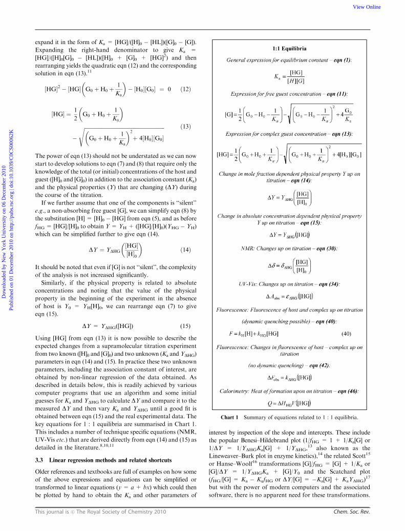
expand it in the form of Ka = [HG]/([H]0 � [HL])([G]0 � [G]).

Expanding the right-hand denominator to give Ka =

[HG]/([H]0[G]0 � [HL])([H]0 + [G]0 + [HG]2) and then

rearranging yields the quadratic eqn (12) and the corresponding

solution in eqn (13).11

½HG�2 � ½HG� G0 þH0 þ1

Ka

� �� ½H0�½G0� ¼ 0 ð12Þ

½HG� ¼ 1

2G0 þH0 þ

1

Ka

� �

�

ffiffiffiffiffiffiffiffiffiffiffiffiffiffiffiffiffiffiffiffiffiffiffiffiffiffiffiffiffiffiffiffiffiffiffiffiffiffiffiffiffiffiffiffiffiffiffiffiffiffiffiffiffiffiffiffiffiffiffiffiffiffiffiG0 þH0 þ

1

Ka

� �2

þ 4½H0�½G0�

s ð13Þ

The power of eqn (13) should not be understated as we can now

start to develop solutions to eqn (7) and (8) that require only the

knowledge of the total (or initial) concentrations of the host and

guest ([H]0 and [G]0) in addition to the association constant (Ka)

and the physical properties (Y) that are changing (DY) duringthe course of the titration.

If we further assume that one of the components is ‘‘silent’’

e.g., a non-absorbing free guest [G], we can simplify eqn (8) by

the substitution [H] = [H]0 � [HG] from eqn (5), and as before

fHG = [HG]/[H]0 to obtain Y= YH + ([HG]/[H]0)(YHG� YH)

which can be simplified further to give eqn (14).

DY ¼ YDHG½HG�½H�0

� �ð14Þ

It should be noted that even if [G] is not ‘‘silent’’, the complexity

of the analysis is not increased significantly.

Similarly, if the physical property is related to absolute

concentrations and noting that the value of the physical

property in the beginning of the experiment in the absence

of host is Y0 = YH[H]0, we can rearrange eqn (7) to give

eqn (15).

DY = YDHG([HG]) (15)

Using [HG] from eqn (13) it is now possible to describe the

expected changes from a supramolecular titration experiment

from two known ([H]0 and [G]0) and two unknown (Ka andYDHG)

parameters in eqn (14) and (15). In practice these two unknown

parameters, including the association constant of interest, are

obtained by non-linear regression of the data obtained. As

described in details below, this is readily achieved by various

computer programs that use an algorithm and some initial

guesses for Ka and YDHG to calculate DY and compare it to the

measured DY and then vary Ka and YDHG until a good fit is

obtained between eqn (15) and the real experimental data. The

key equations for 1 : 1 equilibria are summarised in Chart 1.

This includes a number of technique specific equations (NMR,

UV-Vis etc.) that are derived directly from eqn (14) and (15) as

detailed in the literature.8,10,11

3.3 Linear regression methods and related shortcuts

Older references and textbooks are full of examples on how some

of the above expressions and equations can be simplified or

transformed to linear equations (y = a + bx) which could then

be plotted by hand to obtain the Ka and other parameters of

interest by inspection of the slope and intercepts. These include

the popular Benesi–Hildebrand plot (1/fHG = 1 + 1/Ka[G] or

1/DY = 1/YDHGKa[G] + 1/YDHG,13 also known as the

Lineweaver–Burk plot in enzyme kinetics),14 the related Scott15

or Hanse–Woolf16 transformations [G]/fHG = [G] + 1/Ka or

[G]/DY = 1/YDHGKa + [G]/Y0 and the Scatchard plot

(fHG/[G] = Ka � KafHG or DY/[G] = �Ka[G] + KaYDHG)17

but with the power of modern computers and the associated

software, there is no apparent need for these transformations.

Chart 1 Summary of equations related to 1 : 1 equilibria.

Dow

nloa

ded

by N

ew Y

ork

Uni

vers

ity o

n 06

Dec

embe

r 20

10Pu

blis

hed

on 0

1 D

ecem

ber

2010

on

http

://pu

bs.r

sc.o

rg |

doi:1

0.10

39/C

0CS0

0062

KView Online

Chem. Soc. Rev. This journal is c The Royal Society of Chemistry 2010

More importantly, there are two key problems associated

with using these linear transformations that make their use

highly questionable: (i) they violate some of the fundamental

assumption of linear regression by distorting the experimental

error18,19 and (ii) they frequently involve assumptions and

shortcuts such as assuming that [G] E [G]0 (i.e., the guest is in

large excess) or YHG = Y at the end of titration (i.e., the

complex is fully formed at the end of titration which would

then help to give YDHG)—assumptions that more often than

not can break down and distort the results. The non-linear

regression approach using eqn (14) and (15) with exact

solutions of the quadratic eqn (10) and (12), produces the most

accurate results. This approach is not difficult with modern

computer technology and there is no real excuse for using

old-fashion linear transformations anymore!

The only legitimate use of linear transformations such as the

Scatchard plot is to use them as an aid to visualise the results

after the Ka and [G] have been calculated from non-linear

regression as the human eye finds it easier to detect deviations

in straight lines than variations in hyperboles.19

3.4 The 1 : 2 system

Having defined the 1 : 1 host–guest system, it is relatively

straightforward to proceed with the more complex scenarios.

The derivation of the key equations for 1 : 2 equilibria summarised

in Chart 2 has been detailed previously11 and will not be

repeated here. The key equation here to note is the cubic

eqn (16) as well as eqn (17) and (18) which are analogous to

eqn (14) and (15) for a 1 : 1 system. The latter two equations

describe the expected changes in physical properties upon

titration of a host with a guest in a 1 : 2 system (assuming

again that the guest is ‘‘silent’’, i.e., YG = 0).11 The

experimental data can now be fitted by non-linear regression

to eqn (17) or (18), and the underlying eqn (16), to obtain the

unknown parameters K1, K2, YDHG and YDHG2.

The cubic eqn (16) is of special note here as it has three

solutions which may or may not include complex numbers.

The smallest positive real solution is the only one of relevance

here and as described below, it can be obtained by certain

algorithms in a number of software packages. Once the

concentration of [G] is known, the concentration of [H] can

also be calculated if necessary from eqn (19).11

½H� ¼ ½H�01þ K1½G� þ K1K2½G�2

ð19Þ

3.5 The 2 : 1 system

In principle, the host and guest can be defined at will, but if we

stick to the definition that the concentration of the host is kept

constant then a 2 : 1 host–guest complex would be different

from the 1 : 2 complex discussed above. It is also important to

distinguish the 2 : 1 system from a 1 : 2 system for the same

host, e.g., in the case of cyclodextrins which have been

reported to form 2 : 1, 1 : 1 and 1 : 2 systems to the same

guest depending on experimental conditions (making the data

analysis extremely difficult).10

The 2 : 1 host–guest system can be described by switchingH

and G in eqn (3), eqn (4). The key equations, eqn (20)–(22)

obtained, are summarised in Chart 3. These equations are

derived in a manner similar to the 1 : 1 and 1 : 2 equilibria,

noting also the relevant mass balance eqn (23) and (24).

[H]0 = [H] + [HG] + 2[H2G] (23)

[G]0 = [G] + [HG] + [H2G] (24)

The cubic eqn (20) is analogous to eqn (16) and describes the

concentration of free host [H]. The equations analogous to

Chart 2 Summary of equations related to 1 : 2 equilibria.

Dow

nloa

ded

by N

ew Y

ork

Uni

vers

ity o

n 06

Dec

embe

r 20

10Pu

blis

hed

on 0

1 D

ecem

ber

2010

on

http

://pu

bs.r

sc.o

rg |

doi:1

0.10

39/C

0CS0

0062

KView Online

This journal is c The Royal Society of Chemistry 2010 Chem. Soc. Rev.

eqn (17) and (18) would, however, be slightly different assum-

ing again that the guest is ‘‘silent’’ (YG = 0) as shown in

eqn (21) and (22).

3.6 Cooperativity

In the above discussion on 1 : 2 and 2 : 1 systems the relation-

ship of stepwise binding constants K1 and K2 and how these

are related to Ka for a simple (related) 1 : 1 host–guest system

have not been explored. Taking the 1 : 2 system as an

example, we start with an empty ditopic host (H) with two

identical binding sites which we label A and B (Fig. 3). When

the first guest (G) binds to this host, it can either bind to site A

to form a HG1A0B (the prime 0 indicates which site is occupied)

complex or to site B to form HG1AB0, with the equilibria

described by the binding constants K1A and K1B, respectively.

When the second G binds to the remaining sites inHG1A0B and

HG1AB0, the product in both cases is HG2A02B0, described by

the binding constants K2A and K2B (Fig. 3).

If the binding sites A and B are truly identical we cannot of

course distinguish HG1A0B and HG1AB0 and hence, determine

K1A and K1B (or K2A and K2B) as the physical changes

analogous to, e.g., YHG in eqn (7) for sites A and B in HG

are identical. Although the binding constants K1A, K1B,

K2A and K2B cannot be measured directly they can be related

to the overall stepwise constants K1 and K2. Starting with

eqn (3), we see that [HG] = [HG1A0B] + [HG1AB0] and hence

K1 = K1A + K1B. Likewise, from eqn (4) it is possible to show

that K2 = K2AK2B/(K2A + K2B). If the binding sites A and B

are identical, then it follows immediately that K1A = K1B = K1m

and K2A = K2B = K2m, with K1m and K2m the first and

second microscopic binding constants. Although these cannot

be measured directly, we can see from the above that

K1 = 2K1m and K2 = K2m/2. Conceptually, the factor of 2

in these relations can be explained on kinetic grounds (see also

Section 3.1) as there are two ways for G to bind to the empty

HAB so that the observed on-rate (k1) appears twice as fast

while there are two ways for the G to come off (k�2) the

complex HG2A0B0. If we furthermore assume that there is

no change in the empty remaining site in HG1A0B or HG1AB0

and no specific interaction (e.g. electrostatic) between two

molecules of G bound to HG2A0B0, then K1m = K2m which

describes classical non-cooperative binding in a 1 : 2 system.

We see now that for such non-cooperative binding the stepwise

binding constants K1 and K2 are related by eqn (25).10,20

K1 = 4K2 (25)

This equation is a special case of a more generalised equation

formally defining the expected relationship between stepwise

binding constants in any non-cooperative system, i.e. a system

where the binding sites are truly identical and independent of

each other.21 If the binding of the first G to HG1A0B or HG1AB0

does change the binding properties of the remaining site or

there is some interaction between the two G bound to

HG2A0B0(such as electrostatic repulsion), then K1m a K2m

which describes cooperative binding. We can quantify the

extent of this cooperativity with the interaction parameter

a according to eqn (26).10,20

a ¼ 4K2

K1ð26Þ

Chart 3 Summary of equations related to 2 : 1 equilibria.

Fig. 3 A schematic explaining the microscopic (K1A, K1B, K2A and K2B)

association constants involved in the stepwise formation of a 1 : 2

complex.

Dow

nloa

ded

by N

ew Y

ork

Uni

vers

ity o

n 06

Dec

embe

r 20

10Pu

blis

hed

on 0

1 D

ecem

ber

2010

on

http

://pu

bs.r

sc.o

rg |

doi:1

0.10

39/C

0CS0

0062

KView Online

Chem. Soc. Rev. This journal is c The Royal Society of Chemistry 2010

If a > 1 the system displays positive cooperativity, if a o 1 it

displays negative cooperativity and if a = 1, we arrive at

eqn (25) describing non-cooperative binding.20 The interaction

parameter a can also be used to describe cooperativity (or lack

of it) in 2 : 1 binding system; an a > 1 would suggest that the

formation of a 2 : 1 complex is favourable over the formation

of a 1 : 1 complex.22 When fitting suspected 1 : 2 (or 2 : 1)

titration data to quantitative descriptions such as eqn (17)

it is good practice to fit the data to both a non-cooperative

1 : 2 model, with K1 fixed as 4 � K2 (or vice versa) as well as

cooperative 1 : 2 model where both K1 and K2 are optimised

simultaneously. Using methods described below, the results

should then be compared in order to evaluate if the system of

interest does display true cooperative behaviour. There are

various methods in the literature for plotting data from

cooperative systems, including the above mentioned Scathard

and the Hill which is a log–log plot of the fraction of bound

[H]/free [H] sites against free [G] that are both popular for the

analysis of biomolecular binding.12,23 These methods have

limited value in classical supramolecular titration studies as

they require that the free concentration of the guest and host

can be measured directly.

Co-operativity is not only observed in these simple

homotropic (both guests are the same) systems but also in

heterotropic (the two guests are not the same) 1 : 2 or 2 : 1

systems as highlighted in Fig. 1b.6,7 The more complicated

definitions of co-operativity that apply to these and other

systems such as aggregation (self-assembly) have recently been

reviewed24 and will not be discussed here further.

3.7 More complex systems

Although outside the scope of this tutorial review, similar

approaches can be used to develop equations for more complex

equilibria but not only do these become computationally difficult

(solving a quadric or even quintic equations) but also because the

increased number of unknown parameters (K1, K2, K3. . .) makes

it difficult to get any meaningful results from the fitting process.

Here, simplifications become a necessity. An illustrative example

comes from studies on the so-called sandwich 2 : 2 complexes first

reported by Anderson.22 For a more detailed discussion about

this and other more complex cyclic system the reader is referred to

the excellent work of Ercolani.25

4. Determination of stoichiometry

The execution and analysis of a supramolecular titration experi-

ment is heavily dependent on having at least some knowledge of

what the stoichiometry ratio,m/n in eqn (2), of host and guest is.

Ultimately, one of the main aims of any supramolecular titration

experiment will also be to determine the stoichiometry of the

system under study with the titration data itself providing a key

piece in that puzzle. There are no magical solutions to this

challenge but as Connors suggested,10 a good starting point is to

assume a simple 1 : 1 stoichiometry and then look for other

evidence to support or contradict that assumption. Connors lists

a number of possible methods that can be used including:10

(i) The method of continuous variations (Job’s method).

(ii) Comparison of stability constants evaluated by different

methods,26 including solubility diagrams.

(iii) Consistency with the host structure and available

information on the host–guest complex structure.

(iv) Specific experimental evidence such as isosbestic

point(s).

(v) Constancy of stability concentration as the concentra-

tion is varied, that is, the success of a stoichiometric model to

account for the data.

Of these, the Job’s method has gained significant popularity

to the point of that researchers have started to ignore looking

at other methods to verify stoichiometry even in situations

where the Job’s method is not appropriate. The idea behind it is

simple; the concentration of a HmGn ([HmGn]) complex is at

maximum when the [H]/[G] ratio is equal to m/n.8,11 To

do this, the mole fraction (fG) of the guest is varied while

keeping the total concentration of the host and guest constant

([H]0 + [G]0 = constant). The concentration of the host–guest

complex [HmGn] is then plotted against the mole fraction fGyielding a curve with a maxima at fG = n/(m + n), which in

the case of m = n (e.g., 1 : 1) appears at fG = 0.5.11

In practice, determining the concentration of [HmGn] experi-

mentally may not be straightforward as discussed in Section

3.2. Instead, a property, such as NMR chemical shift or

UV-Vis absorption peak, that seems to have linear dependence

on [HmGn] is used and plotted against fG. For NMR titrations

the approach used by Crabtree is typical of this approach as

[HmGn] is approximated according to eqn (27).27

½HmGn� ¼Dd½H�0

dHmGn � dHð27Þ

The problem here of course is that only at infinite concentra-

tion of [G]0 (when the system is fully saturated) can one obtain

an accurate value for dHmG, although a reasonable estimate

can be obtained by extrapolating the observed dobs at

high [G]0/[H]0 ratios. Generally speaking though, the Job’s

method does work well when there is only one type of complex

(e.g., 1 : 1) present.10 When there is more than one complex

present, the Job’s method becomes unreliable.10,28 This includes

many situations with m/n = 1 : 2 or 2 : 1 as these usually

include two forms of complexes (e.g., HG and HG2) that have

different physical properties, hence the assumption that the

physical property of interest (e.g., dobs) is linearly dependent

may not be valid. For similar reasons, the Job’s method is

likely to fail when either the host or guest aggregates in

solution.9

When Job’s method fails to confirm the simple assumption

about 1 : 1 complexation, one must resort to one or preferably

more of methods (ii)–(v) above. The first of these, Method

(ii) is very useful when supramolecular titrations are combined

with other approaches to determine association constants,

including kinetic measurements and solubility studies.26

Solubility studies do though require significant quantities of

host (and guest), explaining perhaps why this method has

fallen out of favour as the synthetic sophistication of the hosts

used in supramolecular chemistry increased in recent times.

Method (iii) is perhaps the simplest but often the most

effective of all the approaches available to determine the

stoichiometry in host–guest complexes. In modern supra-

molecular chemistry it is now rare not to have detailed

information through X-ray crystallography, 2D-NMR and

Dow

nloa

ded

by N

ew Y

ork

Uni

vers

ity o

n 06

Dec

embe

r 20

10Pu

blis

hed

on 0

1 D

ecem

ber

2010

on

http

://pu

bs.r

sc.o

rg |

doi:1

0.10

39/C

0CS0

0062

KView Online

This journal is c The Royal Society of Chemistry 2010 Chem. Soc. Rev.

Molecular Modelling about the structure of the host and guest

and in some cases even the host–guest complex itself. This

structural information can make the prediction of stoichio-

metry quite straightforward and accurate.

Method (iv) relies on specific evidence such as isosbestic

points which can be used to confirm that more than one type

of complex is present and hence that simple 1 : 1 complexation

is not appropriate to describe the system if more than one

isosbestic point is observed.8 The converse is not necessarily

true, i.e. the absence of more than one isosbestic point cannot

be used to rule out more complex stoichiometry such as 1 : 2

complex formation, especially in cases where the cooperative

(positive or negative) processes play a significant role.

Connors points out that Method (v) is probably the most

generally applicable method for determining stoichiometry.

Firstly, if anything other than 1 : 1 stoichiometry is suspected,

the data should be fitted to other plausible models (e.g., 1 : 2)

and the quality of fit of the different models compared in details,

taking into account factors such as the increase in parameters in

the fitting process (see also Section 6.2 below). Secondly, and

more importantly, it is strongly advisable to carry out the

titration at different concentrations and even with different

techniques (e.g., NMR and UV-Vis). If a particular model is

successful at explaining the data at different concentrations then

it can be taken as very strong evidence for that model.

Finally it is worth mentioning the mole ratio method11

which essentially uses an ordinary binding isotherm from a

titration study where the concentration of [H]0 is fixed and the

concentration of [G]0 is varied. The apparently linear portions

at the beginning and the end of the curve are extrapolated to

find a break point, corresponding to the point of the isotherm

with the most abrupt change. This break point usually corres-

ponds to the [G]0/[H]0 stoichiometric ratio and is especially

useful for non-cooperative higher-order complexes. This

method needs to be applied with care if the system is likely to

display significant levels of cooperativity or if the physical

changes between the different levels of complexation (e.g., the

H2G and HG complex) are non-linear. Some software packages

try also to find the stoichiometry essentially by introducing the

n/m ratio as one of the parameters to fit. The n/m is then reported

back as a real number which essentially can take on any value

between 0 and infinity. This makes sense when studying the

binding of small guests to large (bio)macromolecules such as

proteins and DNA. Two notes of caution need to be raised here:

firstly, most of these software models assume no cooperativity—

an assumption that is not always appropriate. Secondly, a

non-integer n/m value does of course not describe the real

system—e.g., a host will either bind 1 or 2 cations but not 1.3

(there is no host with 0.3 binding sites)! A better approach is to

use the results from these programs as a starting point for further

analysis of the stoichiometry.

5. Common techniques for supramolecular

titrations

5.1 General consideration and preparation of solutions

It is hopefully now clear from the above that a proper

understanding of how association constants are determined

cannot be gained without looking at the underlying

fundamental equilibria and mathematics. In addition, some

chemical understanding of the system under scrutiny is

essential. What sort of association is most likely? Is it probably

a case of 1 : 1 host-to-guest interaction or is there multi-

valency in this system? What influence will this association

have on the host’s physical properties (UV-Vis, fluorescence,

NMR, solubility etc...). Will the host aggregate as well? How

strong are these associations likely to be? It may seem counter-

intuitive to ask such questions as the key purpose of titration

experiments in supramolecular chemistry is usually to get

proper answers to the above questions! The reality is, however,

that having at least some reasonable answer(s) to the questions

above will aid enormously in the design of the titration

experiments, including what technique will be most appropriate

for the titration experiment. In some instances trial titration

experiments covering a large range of concentrations may be

necessary to probe these questions.

When a supramolecular titration study is carried out one

has to first make a decision on what technique is going to be

used to follow the physical changes (DY) in the system during

the course of experiment. The two key concerns here

should be:

i. The expected association constant(s).

ii. The expected physical changes (DY) upon association.

The expected association constant determines what concen-

tration should be chosen for the host system which in turn will

have an influence on the choice of technique. Wilcox,29 using a

parameter defined by Weber as probability of binding or p,30

showed that it is vital to collect as many data point as possible

within the range: 0.2 o p o 0.8 with p defined according to

eqn (28) and (29).

p ¼ ½HG�½G�0

when ½H�0 � ½G�0 ð28Þ

p ¼ ½HG�½H�0

when ½H�0o½G�0 ð29Þ

Using eqn (13) from Section 3.2, it is possible to calculate

p for a range of [H]0, [L]0 and Ka values. When the results

are plotted for three fixed [H]0 concentration ranges

(10�3 M, 10�5 M, 10�7 M) as a function of Ka and [L]0/[H]0(equivalents of guest added) typically employed in NMR,

UV-Vis and fluorescence spectroscopy studies, respectively, a

revealing pattern appears (Fig. 4) with the shaded areas

indicating p in the range of 0.2–0.8 (note that this applies only

to 1 : 1 binding systems).

Here it is helpful to introduce the concept of the dissociation

constant: Kd = 1/Ka—the inverse of the association constant

Ka. The Kd values are plotted for reference on the right-hand

y-axis in Fig. 4 (a thick horizontal line indicated where

Kd = [H]0).With this in mind, one can look at three quite

different regions in Fig. 4.

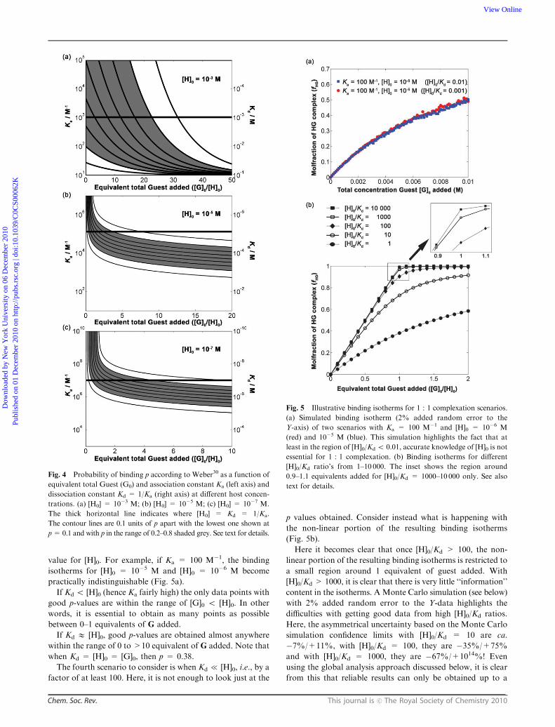
If Kd > [H]0 (hence Ka fairly low) then a relatively large

excess of [G]0 is required to obtain good p-values. In this

situation it would be advisable to collect several data points

in the range of 1–50 equivalents of G added. Interestingly, if

[H]0/Kd > 100, it is not always necessary to have an accurate

Dow

nloa

ded

by N

ew Y

ork

Uni

vers

ity o

n 06

Dec

embe

r 20

10Pu

blis

hed

on 0

1 D

ecem

ber

2010

on

http

://pu

bs.r

sc.o

rg |

doi:1

0.10

39/C

0CS0

0062

KView Online

Chem. Soc. Rev. This journal is c The Royal Society of Chemistry 2010

value for [H]0. For example, if Ka = 100 M�1, the binding

isotherms for [H]0 = 10�5 M and [H]0 = 10�6 M become

practically indistinguishable (Fig. 5a).

If Kd o [H]0 (hence Ka fairly high) the only data points with

good p-values are within the range of [G]0 o [H]0. In other

words, it is essential to obtain as many points as possible

between 0–1 equivalents of G added.

If Kd E [H]0, good p-values are obtained almost anywhere

within the range of 0 to >10 equivalent of G added. Note that

when Kd = [H]0 = [G]0, then p = 0.38.

The fourth scenario to consider is when Kd { [H]0, i.e., by a

factor of at least 100. Here, it is not enough to look just at the

p values obtained. Consider instead what is happening with

the non-linear portion of the resulting binding isotherms

(Fig. 5b).

Here it becomes clear that once [H]0/Kd > 100, the non-

linear portion of the resulting binding isotherms is restricted to

a small region around 1 equivalent of guest added. With

[H]0/Kd > 1000, it is clear that there is very little ‘‘information’’

content in the isotherms. A Monte Carlo simulation (see below)

with 2% added random error to the Y-data highlights the

difficulties with getting good data from high [H]0/Kd ratios.

Here, the asymmetrical uncertainty based on the Monte Carlo

simulation confidence limits with [H]0/Kd = 10 are ca.

�7%/+11%, with [H]0/Kd = 100, they are �35%/+75%

and with [H]0/Kd = 1000, they are �67%/+1014%! Even

using the global analysis approach discussed below, it is clear

from this that reliable results can only be obtained up to a

Fig. 4 Probability of binding p according to Weber30 as a function of

equivalent total Guest (G0) and association constant Ka (left axis) and

dissociation constant Kd = 1/Ka (right axis) at different host concen-

trations. (a) [H0] = 10�3 M; (b) [H0] = 10�5 M; (c) [H0] = 10�7 M.

The thick horizontal line indicates where [H0] = Kd = 1/Ka.

The contour lines are 0.1 units of p apart with the lowest one shown at

p=0.1 and with p in the range of 0.2–0.8 shaded grey. See text for details.

Fig. 5 Illustrative binding isotherms for 1 : 1 complexation scenarios.

(a) Simulated binding isotherm (2% added random error to the

Y-axis) of two scenarios with Ka = 100 M�1 and [H]0 = 10�6 M

(red) and 10�5 M (blue). This simulation highlights the fact that at

least in the region of [H]0/Kd o 0.01, accurate knowledge of [H]0 is not

essential for 1 : 1 complexation. (b) Binding isotherms for different

[H]0/Kd ratio’s from 1–10 000. The inset shows the region around

0.9–1.1 equivalents added for [H]0/Kd = 1000–10 000 only. See also

text for details.

Dow

nloa

ded

by N

ew Y

ork

Uni

vers

ity o

n 06

Dec

embe

r 20

10Pu

blis

hed

on 0

1 D

ecem

ber

2010

on

http

://pu

bs.r

sc.o

rg |

doi:1

0.10

39/C

0CS0

0062

KView Online

This journal is c The Royal Society of Chemistry 2010 Chem. Soc. Rev.

[H]0/Kd = 100—beyond that only a very crude estimation of

the lower limit for Ka can be obtained.

From all the above, it is obvious that with the exception

of very weakly bound systems, data points in the range of

0–1.5 equivalents of G added are usually the most important

data points. There is no fixed rule on how many points should

be collected but in the experience of this author, 10 is the bare

minimum with 15–20 a desirable target for 1 : 1 binding

(especially if the binding is more complex). If there is some

prior knowledge on the strength of binding, a good strategy is

to collect at least 8–10 points between 0–1.5 equivalents of G

and then another 10–15 points spaced non-linearly between

1.5–50 equivalents of G added. Alternatively, when the

strength of binding is completely unknown, one can increase

the guest concentration exponentially, e.g., by increasing the

concentration of [G]0 by a factor of 3 on every addition,

starting at 0.1 equivalents and going up to the highest possible

concentration. After about 1–15 addition, the resulting data

will cover 3–4 orders of magnitude of the [G]0/[H]0 ratio and

hence complexation should be detected somewhere on that

scale even in cases when Kd > 1000 � [H]0.

In the case of 1 : 2 (and 2 : 1) equilibria the situation is

even more complex due to (possible) cooperative effects and

differences in the physical properties being measured, that is

YDHG = YHG � YH and YDHG2in eqn (17) and (18). As an

example let’s look a few possible scenarios for a UV-Vis

titration where the total host concentration [H]0 = 10�5 M

(Fig. 6).

Inspection of Fig. 6 reveals a number of interesting

phenomena. Firstly, looking at the distribution of the two

different complexes in solution (Fig. 6b), we see that for the

statistical binding and positive co-operativity scenarios, the

concentration of the 1 : 2 complex HG2 only reaches above a

mole fraction of 0.2 (roughly corresponding to p > 0.2 above)

once about 2–3 equivalents of G have been added. In the

negative co-operativity case, over 10 equivalents are needed to

reach a mole fraction of 0.2. In contrast the intermediate 1 : 1

complex HG is most pronounced between 1–10 equivalents of

G except in the case of positive cooperative binding. The latter

observation suggests that for highly positive cooperative

systems, the detection of the intermediate 1 : 1 HG complex

can become very difficult.

The situation is further confounded by all the possible

combinations that the changes in molar absorptivity eDHG

and eDHG2, can take. In Fig. 6c, the UV-Vis isotherms for

three possible scenarios for eDHG and eDHG2are plotted for the

three different cooperativity scenarios outlined in Fig. 6a. The

three eDHG and eDHG2scenarios are (i) when eDHG and eDHG2

are quite similar (30 000 vs. 20 000), (ii) when the first is

very weak compared to the second (eDHG and = 1000,

eDHG2= 20 000) and finally (iii) when the second has an

opposite almost equal sign to the first (eDHG = 30 000 and

eDHG2= �20 000).

This simulation shows that the differences in molar absorptivity

can have at least the same if not more effect on the resulting

binding isotherm than changes in cooperativity. Further,

unless the signs of the change in molar absorptivity are

opposite, the differences between the binding isotherms are

not that large, especially in the early stages of the titration.

The take-home message from Fig. 6 is that one needs to

obtain as many data points from the whole range of at least

0–10 equivalent of G added as possible, with special emphasis

on the first part of that range.

Finally, having decided on the concentration range and

the number of addition (titration) points to use, it is worth

considering a few tips on how to prepare solutions for

supramolecular titrations. It goes without saying that the

purity of the host and guest is of utmost importance, especially

with optical techniques (UV-Vis, fluorescence etc.) as

small impurities (which may not be detectable by NMR) can

cause peaks to appear (or disappear) unrelated to complex

formation. The concentration of the host should also be

kept constant throughout the titration to avoid compli-

cations arising from (minor) aggregation and the application

of complicating dilution factor corrections in the quantitative

equations used to describe the system of interest.

Fig. 6 Simulated UV-Vis titrations for a 1 : 2 equilibria with

[H]0 = 10�5 M and b12 = K1K2 = 109 M�2. (a) Colour coding for

the three different scenarios: blue = positive co-operativity (a = 40),

black = statistical binding (a = 1) and red = negative co-operativity

(a = 0.025). (b) Mole fraction distribution of [H], [HG] and [HG2]

(see arrows). (c) The resulting UV-Vis binding isotherms depending on

three possible scenarios for eDHG and eDHG2(see arrows). Note

that two of the binding isotherms for the negative co-operativity

(a = 0.025) scenario coincide. See also text for details.

Dow

nloa

ded

by N

ew Y

ork

Uni

vers

ity o

n 06

Dec

embe

r 20

10Pu

blis

hed

on 0

1 D

ecem

ber

2010

on

http

://pu

bs.r

sc.o

rg |

doi:1

0.10

39/C

0CS0

0062

KView Online

Chem. Soc. Rev. This journal is c The Royal Society of Chemistry 2010

The easiest way to do this is to make up the guest solution

from the same host stock solution used in the titration. In the

case of an NMR titration one could therefore make up a 2 mL

solution of the host at concentration [H]0 and then use 1 mL of

that solution to make up the guest solution at ca. 20–100 fold

higher concentration ([G]0 = 20–100[H]0). The remaining host

solution (ca. 600–1000 mL) is then transferred to an NMR

tube. Note that all these volumes need to be measured

accurately which is preferably done with an accurate micro-

balance (and then convert to volumes using the density of the

solvent) rather than relying on volumetric flasks or pipettes.

The guest solution is then added in small quantities (1–10 mL)to the NMR tube using an accurate microsyringe (such as

Hamiltons syringes for organics or Eppendorfs

pipettes for

aqueous solutions).

5.2 NMR titrations

The most informative technique in most situations is1H NMR. Other forms (13C, 19F etc.) of NMR are also

applicable. Apart from the quantitative information that an

NMR titration can yield, the relative shifts and changes in

symmetry can often give valuable information about how the

host and guest(s) are interacting and the stoichiometry of

interaction. This information can be of significant benefit even

in situations where complete quantitative data cannot be

obtained from the NMR titration as shown in our work on

the binding of a ditopic porphyrin host to viologen where

symmetry changes were indicative of 1 : 1 and 1 : 2 complex

formation.31

Classical approaches for data analysis of NMR titrations

assume that the resonance (d) of interest is the weighted

average of the free host (H) and the bound host in the complex

(HG) in the experiment according to eqn (30) in Chart 1 in the

case of a simple 1 : 1 system.11 We immediately recognise this

as a special case of eqn (13) above in Section 3.2. We can

proceed directly from the relevant equations in Sections 3.4

and 3.5 to the descriptive quantitative expressions that outline

the expected changes in chemical shifts (Dd) assuming a 1 : 2

or 2 : 1 complexation, according to eqn (31) or (32),

respectively (Chart 2).

With modern NMR instruments it is possible to obtain

good quality spectra with sub-millimolar concentrations

(routinely now as low as 10�4 M), suggesting from the above

discussion that NMR might be suitable for Ka up to and even

above 106 M�1. That said, many literature references will state

that 105 M�1 is the limit for NMR titration experiments.29

Here, one has also to take into account the relative exchange

rates within the host–guest or in other words, the previously

mentioned (Section 3.1) relationship between the equilibrium

association constant and the kinetics on/off rates (Ka = k1/k�1)

and the timescale of the NMR experiment. The real limiting

factor for NMR titrations is therefore whether the system of

interest is in the fast or slow exchange region under the

conditions used. Besides the association constants and the

related on/off rate constants, the magnitude of the observed

complexation induced chemical shift (Dd) is related to the mole

fraction of the free host divided by the off rates (fH/k�1) or

equivalently, the combined inverse of the lifetimes of nucleus

of the complex (1/tHG) and the free host (1/tH). It has been

shown that the simple assumptions behind eqn (30) and

related equations break down if the system is not in the fast

exchange region as defined by eqn (33).32

2pjvH � vHGj �1

tHþ 1

tHG

� �ð33Þ

Inspection of eqn (33) shows that it can actually be

beneficial to focus on resonances with relatively small com-

plexation shift (Dd) when analysing titration curves as these

might still be in the fast exchange region while those with

larger Ddmay have broadened out due to slow exchange! That

said, Ka = 105 M�1 remains the usual practical limit for direct

NMR titrations in the fast exchange region (competition

experiments being one notable exception, e.g., the work of

Wilcox et al.).33 It may be tempting to think that in the (very)

slow exchange region of NMR, one could obtain an association

constant directly from the relative ratios of the free and bound

host, however, can be difficult in practice due to complications

that arise in the intermediate-to-slow region with the size

(amplitude) of the observed resonances32 and the usual limita-

tion of obtaining accurate (quantitative) integration from

NMR experiments.

5.3 UV-Vis spectroscopy

The second most common method for supramolecular titra-

tion experiment is probably UV-Vis spectroscopy. With the

right chromophore (e.g., in the case of porphyrins), host

concentration in the sub-micromolar (10�7 M) can be applied,

making the determination of association constants as high as

109 M�1 in simple 1 : 1 systems possible (albeit difficult) with

Kd/[H]0 = 100 as discussed above. The concentrations chosen

must lie within the region where the absorption peak(s) of

interest in both the host and its complex are within the limits

of the Beer–Lamberts Law (A= bce, withAo 1). Additionally,

it is desirable that the guest added does not have any absorp-

tion in the region of interest as this simplifies the system

considerably—fortunately, this is usually the case in simple

supramolecular systems (e.g., upon addition of simple cations

or anions to a host). It is also important that the complexation

causes a notable change in the UV-Vis spectra as the usual

approach for analysis of UV-Vis titration data assumes a

significant change in the molar absorptivity (e) upon com-

plexation according to eqn (34) (Chart 1) which is a special

case of eqn (15) from Section 3.2 above. Similarly, with 1 : 2

and 2 : 1 binding, one obtains eqn (35) (Chart 2) and eqn (36)

(Chart 3) that are derived from eqn (18) and (21).

Although applicable to all the different methods available

(including NMR), titration by UV-Vis spectroscopy is

particularly vulnerable to dilution and temperature effects

(all supramolecular titration experiments need some tempera-

ture control) and the presence of impurities in either host or

guest solutions. If a low concentration of the host is required,

special care needs to be taken in weighing out samples

and solutions so that the concentration of the host can still

be determined with good accuracy. In certain situations

(e.g., when only minute quantities of host are available) it is

not possible to accurately determine the concentration of the

Dow

nloa

ded

by N

ew Y

ork

Uni

vers

ity o

n 06

Dec

embe

r 20

10Pu

blis

hed

on 0

1 D

ecem

ber

2010

on

http

://pu

bs.r

sc.o

rg |

doi:1

0.10

39/C

0CS0

0062

KView Online

This journal is c The Royal Society of Chemistry 2010 Chem. Soc. Rev.

host and the host concentration must then be included as one

of the unknown parameters in the fitting process. It should

also be noted again that when [H]0/Kd > 100, it is not

necessary to have an accurate value for [H]0 in the case of

1 : 1 binding (Fig. 5a).

5.4 Fluorescence spectroscopy

The third most popular and perhaps the most sensitive

technique is fluorescence (and other related luminescence)

spectroscopy. The phenomenal sensitivity of this technique

makes routine measurements in the sub-micromolar, even

nanomolar (nM) range possible and hence, fluorescence

spectroscopy is ideal for the determination of very large

association constants (Ka > 106 M�1). In fact, fluorescence

titration must be carried out at relatively low concentration or

ideally where the absorbance at the excitation wavelength used

is less than 0.05 (A o 0.05). Above these concentrations the

fluorescence response (F) is no longer linearly dependent on

the light absorbed. Additionally, inner filter effects will also

cause deviations from linearity at higher concentration.34 The

observed fluorescence at low concentration of a species X can

usually be described by eqn (37).34

F = I0Feb[X] = kX[X] (37)

Fluorescence is a particularly useful technique in the case

when only one of the species in solution is fluorescently active,

i.e. when either the free host or guest is fluorescent ‘‘silent’’ or

inactive and the fluorescence of the remaining species is either

turned ‘‘off’’ (quenched) or ‘‘on’’ upon complexation. If

quenching plays a role, it is necessary to differentiate between

static and dynamic (collisional) quenching, with only the

former of real significance for supramolecular binding studies.

Dynamic quenching is usually measured by plotting the ratio

of the initial (F0) and measured (F) fluorescence intensity

ratio (F0/F) against the concentration of the quencher [Q]

according to the Stern–Volmer relation F0/F = 1 + KSV[Q],

with KSV = the Stern–Volmer constant. Unfortunately, pure

1 : 1 static quenching follows a nearly identical relation:

F0/F = 1 + Ka[Q], with [Q] = the free concentration of the

quencher (guest) and Ka is of course the familiar association

constant of interest in supramolecular binding studies. In

many cases the observed quenching is a mixture of both static

and dynamic quenching which can lead to some complication

in the analysis of the titration data. With this in mind, there

are three general scenarios that need to be taken into account

when analysing data from supramolecular fluorescence titra-

tions (we will skip here the derivation for the 1 : 2 and 2 : 1

systems—these can be derived from the generic relations in

Section 3—see Charts 2 and 3).

The most simple case is the situation when only the

complex formed is fluorescent (complexation turns fluores-

cence on) with the observed fluorescence described by

eqn (38).

F = kHG[HG] (38)

The next scenario is when both the free host and the

complex are fluorescent. Before any guest is added to the

solution the observed fluorescence can be described by

eqn (39).10

F0 = k0H[H]0 (39)

After the addition of a guest, the resulting fluorescence will

follow eqn (40).10

F = kH[H] + kHG[HG] (40)

It is important to recognise that k0H may not be equal to

kH, essentially due to complications arising from dynamic

quenching of the free host. Many researchers find it convenient

to combine eqn (39) and (40) with the aid of eqn (9) to get

eqn (41).10

F

F0¼ kH=k

0H þ ðkHG=k

0HÞKa½G�

1þ Ka½G�ð41Þ

In the special situation where the complex is fluorescently

silent (quenched) and k0H = kH (no dynamic quenching) we

obtain an equation that looks identical to the Stern–Volmer

equation describing classical static quenching according to

eqn (42).10

F0

F¼ 1þ Ka½G� ð42Þ

Likewise, if kH0 = kH (no dynamic quenching of the host) but

the complex is still fluorescently active (kHG a 0) we can use

the generic approach from Section 3.2 with eqn (15), to obtain

eqn (43).

DFobs = kDHG([HG]) (43)

With DFobs = Fobs� F0, the observed fluorescence change and

kDHG = kHG � kH, the change in the proportionality constant

between the complex and the free host.

Obviously, eqn (43) is almost identical to eqn (34) for UV-Vis

titration and provided that the assumption k0H = kH is valid

one can also derive equations similar to eqn (35) and (36) to

describe 1 : 2 and 2 : 1 binding for fluorescence titrations

according to eqn (44) (Chart 2) and eqn (45) (Chart 3).

5.5 Other methods and summary of techniques for

supramolecular titrations

The three examples above in combination with the general

equations in Section 3 can be used to develop expressions for

almost any supramolecular titration techniques imaginable.

Calorimetry represents a powerful example of other methods

used in supramolecular titration. This technique relies on

measuring enthalpy (H) increases on the addition of a guest to

a host in a specially designed apparatus measuring the heat (Q)

formed or absorbed (usually a isothermal calorimeter—ITC).

After taking care of eliminating dilution effects (see also above

in Section 5.1), the heat measured is simply related to the

molar enthalpy (DH) multiplied by the number of moles of the

complex formed which can be obtained from the molar

concentration of the complex ([HG]) and the volume of

solution (V). Hence in the case of a simple 1 : 1 equilibria

we again use eqn (15) from Section 3.2 above to obtain

eqn (46) (Chart 1). Similarly, with 1 : 2 and 2 : 1 binding

Dow

nloa

ded

by N

ew Y

ork

Uni

vers

ity o

n 06

Dec

embe

r 20

10Pu

blis

hed

on 0

1 D

ecem

ber

2010

on

http

://pu

bs.r

sc.o

rg |

doi:1

0.10

39/C

0CS0

0062

KView Online

Chem. Soc. Rev. This journal is c The Royal Society of Chemistry 2010

one obtains eqn (47) and (48) that are derived from eqn (18)

and (21).

The most powerful feature of calorimetric titrations is

that not only does it yield the free energy (DG) changes via

the association constant according to eqn (49) but also the

enthalpy and thus the entropy (DS) change can also be

obtained from eqn (50).

DG = �RTln(K) (49)

DG = DH � TDS (50)

6. Data analysis and interpretation

6.1 Fitting data: choosing a model, software considerations

and global analysis

Having done all the hard work to obtain the supramolecular

titration one might hope that analysing it was as simple as

pressing a button on a computer. However, this is not the case,

even with the most sophisticated data analysis software. Many

chemists would be familiar with a similar situation from the

field of computational chemistry; with modern modelling

software it might look easy to build a molecule and optimise

its structure but the fact still is that unless you understand

reasonably well the way you enter the initial model, set up the

simulation, which force field or DFT basis set you use and so

on, the final results may not be worth all that much. The

parallels don’t end there: in the past most people in both

fields had to write their own software code whereas now

commercially available software packages appear to make

the task more straightforward. This still doesn’t exclude

researchers from trying to understand what the key steps are.

Briefly, the process could be divided into: choosing a

model, making adjustment to the model, transforming data

(if necessary), weighing data, deciding on whether to use

global analysis, choosing a minimisation algorithm, initial

guesses of parameters, iteration, displaying and plotting

results and analysing the quality of the fit obtained. Covering

all of these aspects of data analysis is beyond the scope of this

tutorial review, but here the focus will be a few key aspects of

this process including: choosing and making adjustments to

model, some software considerations and global analysis. The

following section will the discuss how to analyse the quality of

fit and estimation of uncertainties. For more details and other

aspects of data fitting, interested readers are encouraged to

read the work of Motulsky.18,19

In Section 4 it was emphasised that sometimes the best

approach involves actually trying two or more approaches.

The case of suspected 1 : 2 equilibria is a classic example.

Comparing eqn (13) and (34) (Chart 1) with eqn (16) and (36)

(Chart 2) shows that we have only 2 parameters to fit UV-Vis

data to a 1 : 1 model (Ka and eDHG) while there are up to four

in the case of a 1 : 2 model (K1, K2, eDHG and eDHG2). However,

if we assume that the 1 : 2 binding is statistical, we can fix

K2 = 4K1, reducing the number of parameters by one.

Naturally, the model with the highest number of parameters

(cooperative 1 : 2 binding) should give us the best fit. What we

must do is to fit the data to all three models (1 : 2 cooperative,

1 : 2 statistical and 1 : 1 binding) and then compare the

overall quality of fit. Only if going from a simple (1 : 1) to a

more complex (e.g., cooperative 1 : 2) model gives truly

significant improvements in fitting can we justify our choice

of that model.

Choosing and sometimes modifying a model is the first crucial

step. The key issue to be aware of is that the more parameters

you fit, the better the fit will be. Almost any data could be fitted

to a polynomial equation (y= a+ bx+ cx2 + dx3 + � � �) if itis expanded to high enough nth-order. This doesn’t mean that

it has any physical meaning. On the other hand there is

sometimes a valid case for introducing extra parameters, for

instance, to correct a baseline19 or as mentioned, to estimate

the concentration of the host [H]0 when its concentration

and purity are not well established (e.g., in dilute solutions

for UV-Vis).

When it comes to the actual data fitting, there are essentially

two different types of software available: (i) commercial software

packages dedicated to fitting data to binding models such as

GraphPads19 and custom written programs that often run as

macros or routines with generic data andmathematical programs

such as Excels, Matlabs or Mathematicas. Commercially

available software packages have the advantage of being

relatively easy to use in terms of loading the data with an output

that usually includes additional information such as residual

plots and estimation of uncertainties (See Section 6.2 below).

Their main drawbacks usually are lack of information about

the underlying equations used in the fitting and data analysis

process. In addition, these packages are usually targeted to

customers in biochemistry or pharmacology, which sometimes

results in NMR titrations being left out. Custom written

packages on the other hand are usually written by people

who are active in the area of supramolecular chemistry and

hence well aligned with the methods discussed here. The

disadvantages of these packages are that they may not have

been verified thoroughly for errors and mistakes. Additionally,

they may not be particularly user friendly, requiring a fairly

high level of software familiarity or even programming

expertise of the user.

Although there is frequently a lot of discussion on the

relative merits of the different minimisation algorithms used

in these software packages, such as the Gauss–Newton,

Marquardt and Simplex,18 the reality is that other features

are usually much more important. To start with, does the

software handle the cubic equations (16) and (20) properly?

These equations can be solved directly in some programs

(e.g., Mathematica and Matlab) but other programs may

employ the method of successive approximation to solve these

equations. The latter approach fails more frequently which

may explain that several software packages do not handle 1 : 2

or 2 : 1 binding models at all (see though Section 6.2). As

we will see below, global analysis is another method that

is particularly useful for dealing with more complex binding

equilibria but this feature is also lacking in many software

packages. An example of a custom written package (for Matlab)

that does provide both a direct solution to eqn (16) and (20)

and global analysis options is provided in the ESIw of this

paper by the author.

Quite often, the titration yields more than one set of data,

for instance in 1H NMR titration where a noticeable shift is

Dow

nloa

ded

by N

ew Y

ork

Uni

vers

ity o

n 06

Dec

embe

r 20

10Pu

blis

hed

on 0

1 D

ecem

ber

2010

on

http

://pu

bs.r

sc.o

rg |

doi:1

0.10

39/C

0CS0

0062

KView Online

This journal is c The Royal Society of Chemistry 2010 Chem. Soc. Rev.

often observed for more than one proton resonance upon

complexation of the host. The same applies to UV-Vis

data—the formation of a complex often leads to one increase

at one particular wavelength while another one is decreasing.

The global analysis method is ideal for analysing this sort of

data. The idea is simple: take a family of data sets that share at

least one parameter and fit them simultaneously. For instance,

if i noticeable shifts in proton resonances up on a 1H NMR

titration are observed, we modify or expand eqn (30) to obtain

eqn (51).

Xnj¼1

Ddi ¼Xnj¼1

dDHGi

½HG�½H�0

� �ð51Þ

Why would we want to do this, especially just after noting that

increasing the number of parameters can artificially make the

fitting process better? Here we need to note that what we

are actually doing is to double the number of data points we

are fitting. But this only explains part of the story as outlined

in an excellent paper by Beechem.35 In simple terms, what

global analysis really does is to tighten the so-called error

surface considerably compared to single-experiment or

local fitting and this more than compensates for the increase

in the number of parameters. The technique is exceptionally

useful in the analysis of multiple equilibria (e.g., 1 : 2 complex

formation).

The benefits of global vs. local fitting of data are best

explained by an example. Here two of the outcomes in Fig. 6

are considered, both having the same binding constants but

different changes in eDHG and eDHG2for these data sets. A little

(�1% standard deviation) random noise is added to the

simulated isotherms and the resulting data fitted as two single

experiments (local fitting) and also globally in line with

eqn (51) as shown in Fig. 7.

The results in Fig. 7 reveal a number of characteristics

of global over other fitting procedures. Firstly, the results

from the global fitting are much closer to the ‘‘true’’ values

(the one used at the start of this simulation) than either of

the two local fits. Secondly the asymptoting standard error

(see cautions about this type of uncertainty estimation below)

is quite acceptable, i.e., less than 20% for all parameters

compared to up to 40%–140% for the two local fits. Thirdly,

contrary to what one might expect, the parameters obtained

from the global fits are not just simply the average of the local

fits (cf., K1). Finally, it is noteworthy that this does not happen

because the overall fit is very different—the isotherms obtained

from the local vs. global fit are very similar (Fig. 7b inset). A

good indicator of the quality of the fit is the standard error of

the y estimate—SEy—which is defined by eqn (52) and related

to chi-squared (w2) in eqn (53).36

SEy ¼

ffiffiffiffiffiffiffiffiffiffiffiffiffiffiffiffiffiffiffiffiffiffiffiffiffiffiffiffiffiffiffiffiffiffiffiPðydata � ycalcÞ2

N � k

sð52Þ

w2 ¼

ffiffiffiffiffiffiffiffiffiffiffiffiffiffiffiffiffiffiffiffiffiffiffiffiffiffiffiffiffiffiffiffiffiffiffiPðydata � ycalcÞ2

N � k� 1

sð53Þ

Interestingly, the SEy is actually not any better (lower) for the

global fit than the better two of the local fits. We also see from

this that having a small change in one of the physical properties

(eDHG), in data set 1 is largely responsible for the poor

results obtained from that local fit. This is because the fitting

processing can alter eDHG almost at will while also varying K1

until a good apparent fit is obtained. The global fitting process

on the other hand has no problems in obtaining a good

estimate for the small change in eDHG while at the same time

uses the underlying data to narrow the error-surface around

K1 and the other parameters in this system. Global analysis is

in fact particularly powerful in dealing with complex situations

such as cooperative 1 : 2 binding systems.

6.2 Evaluating the quality of the fit and estimating uncertainty

The example in Fig. 7 also illustrates the importance of

analysing the quality of the fit obtained. This is not a trivial

matter and there are no rigorous procedures (bullet proof)

to follow here. There are, however, a few basic tests and

Fig. 7 Local vs. global fit for a hypothetical UV-Vis titration for a

1 : 2 complexation equilibria. (a) The initial conditions (see also

Fig. 6), the colour coding for the two different data and the global

fit. The data points (red and blue squares) are generated from eqn (35)

using the parameters shown here with an additional random noise

of �1%. (b) The resulting binding isotherms with the local and global

fits (solid lines) superimposed. The enlarged area (red shaded square)

shows the similarities of the local and global fitted isotherms. (c) The

results from the local and global fitting process with the asymptoting

standard error (see Section 6.3) in parentheses. SEy = standard error

of the y estimate—see eqn (52). See also text for details.

Dow

nloa

ded

by N

ew Y

ork

Uni

vers

ity o

n 06

Dec

embe

r 20

10Pu

blis

hed

on 0

1 D

ecem

ber

2010

on

http

://pu

bs.r

sc.o

rg |

doi:1

0.10

39/C

0CS0

0062

KView Online

Chem. Soc. Rev. This journal is c The Royal Society of Chemistry 2010

strategies that can be applied here.19 The first one is a visual

examination of the fit or more importantly, the residual plot.

This is a plot of yfit, fit for each data point, i.e., the difference

between measured ydata and calculated ycalc in eqn (52), as a

function of the total guest ([G0]) added. Typically yfit is also

normalised by dividing the yfit with SEy in eqn (52). Ideally, the

residual plot should be randomly distributed above and below

zero.37 A systematic trend in the residual plot indicates a poor

fit. The residual plot also helps identifying ‘‘poor’’ data

points,37 which may need to be rejected in further analysis,

especially if magnitude of yfit is greater than 3 � SEy.38

In some situations, physically non-sensible parameters

(very low or very high DY, negative Ka etc.) will suggest that

something is wrong with the model. Here, the researcher will

have to use their background knowledge; a kH = 106 for a

fluorescence titration experiment might make sense while

dDHG = 100 ppm for an 1H NMR titration doesn’t make

sense. In extreme situations, the data simply don’t fit the

model with the software used returning answers such as

‘‘didn’t converge’’, ‘‘Hessian matrix is unstable’’, ‘‘can’t divide

by zero’’. This is in some cases a clear sign that something is

wrong with the program although it is wise to check the fitting

procedure again with different initial guesses.19 Running a

fitting program again with slightly different initial guesses is in

any case a good test of how ‘‘stable’’ or close to the real global

minimum the fitted solution is. In the case of 1 : 2 binding and

more complex situation it is also possible that the program

used doesn’t handle the cubic eqn (16) and (20) leading to a

‘‘false negative’’ results.

If the data fits reasonably to more than one possible binding

model (cf. Section 4), one must try to compare the quality of

the fits in a quantitative fashion. This is quite often non-trivial

and there are many examples where no simple statistical

methods can be applied for this task.19 A natural starting

point for this might be to compare the sum of squared

fits—ssyy = S(ydata � ycalc)2—the parameters usually minimized

in the fitting process. The SEy introduced in eqn (52) is though

probably a better tool as it tries to make some corrections for

the number of parameters used. Another approach that this

author has used is the covariance of the fit,7,9,31 covfit, defined

by eqn (54) as the (co)variance of the residuals (ydata � ycalc)

divided by the (co)variance of the raw data.

covfit ¼covðyfitÞcovðydataÞ

ð54Þ

The covfit gives a numerical representation of how random is

the scatter in the residual plot relative to the scatter in the

original data. This quantity is usually relatively insensitive to

the number of parameters used in the fitting process.

Regardless of what quantity (ssyy, SEy, w2, covfit etc.) is used,

when comparing two models the one that has a larger number

of adjustable parameters (e.g., statistical vs. cooperative 1 : 2

equilibria) will usually seem better (lower). This ‘‘improvement’’

in the fit when increasing the number of parameters can be

misleading. Here it is suggested that only if there is a signifi-

cant (e.g., >2–3 fold) improvement in, say covfit, when

comparing two models, should one select the more complex

model. Other tests, such as F-test can be used provided the

models are nested, i.e., one of the models is a simpler case of

another.19

The final, but perhaps most important step in the data

analysis is the estimation of the uncertainty. Here one might

be tempted to ask if we need to estimate the measurement

uncertainty. The answer is of course yes as it confirms how

reliable the results are—indeed it has been stated that any

analysis without proper information of the reliability is

useless!38

One of the key downsides of non-linear regression analysis is

that there are no straightforward methods for estimating the

uncertainty of the results obtained from it. The ‘‘standard

error’’ reported by most software packages is the so-called

asymptotic standard error.19 This standard error is then used

to calculate 95% confidence intervals (which can be approxi-

mated as the 2 � the standard error). This error is only

‘‘approximate’’ and it also relies on a few key assumptions

regarding the non-linear regression process, including that the

error is only on the physical property (Y) measured. This is

rarely true as there will always be some (or quite large)

uncertainties on the concentrations of the host [H]0 and guest

[G]0—the quantities that form the x-axis in the fitting process

(cf. Fig. 7).

In addition, the very method used to calculate the asymptotic

errors introduces assumptions that are usually not valid for a

supramolecular system. The details are beyond the scope of

this tutorial review but a key step here involves transforming

the regression problem into a matrix equation and then a

matrix inversion resulting in the so-called variance–covariance

matrix. The final results of this assumes that the confidence

interval is symmetrical (+/� are the same) around the

parameter of interest,19 which is probably not true in most

cases. These factors generally result in underestimation of the

realistic uncertainty. Additionally, matrix inversion requires

division with the determinant of the original matrix and

sometimes this determinant is a very small number, resulting

in unstable or even a singular matrix (if determinant is zero).8

The resulting asymptotic error will therefore be meaningless.

This problem is particularly common with more elaborate

equilibria such as 1 : 2 equilibria where the underlying matrix

manipulations are very complex.

A more rigorous but more intensive approach involves some

form of grid search such as the weakened grid search method

proposed by Beechem.35 Here, one parameter is fixed at

different values while all others are optimised in the usual

manner. The resulting ssyy (or w2) is then plotted as a func-

tion of the different values for the fixed parameters and the

F-statistics test is used to determine the increase in ssyy that is

significant at a predetermined confidence interval (e.g., 67%)

for that parameter. The procedure is then repeated for the

other parameters yielding a cross-section of the error surface

for all these parameters of interest. In the full grid search

method all possible combination of the parameters are varied

at certain intervals to map out the error surface and obtain

the confidence intervals via F-statistics, but this method is

quite computationally intensive. Even more intensive but

perhaps most rigorous of these is a Monte Carlo approach

where a random scatter is added to the ‘‘ideal data’’ generated

from the parameters obtained (akin to the isotherms in Fig. 6).

Dow

nloa

ded

by N

ew Y

ork

Uni

vers

ity o

n 06

Dec

embe

r 20

10Pu

blis

hed

on 0

1 D

ecem

ber

2010

on

http

://pu

bs.r

sc.o

rg |

doi:1

0.10

39/C

0CS0

0062

KView Online

This journal is c The Royal Society of Chemistry 2010 Chem. Soc. Rev.

We then add random scatter to this data and optimise again

(as in Fig. 7) and then repeat the procedure n-times to obtain a

statistically meaningful distribution of the fitted parameters.

Taking Data 2 in Fig. 7 as an example, this yields unsymmetrical

and generally a little larger confidence limits for the para-

meters of interest than the one obtained from the asymptotic

error (e.g., for K1 the limits are 97 000–140 000 with the

asymptotic method but 95 000–150 000 with the Monte Carlo

approach). The advantage of this approach is that scatter

can also be applied to x-axis data such as the concentrations of

the host [H]0 and guest [G]0. The disadvantages are the

computational intensity required and the subjective element

involved in deciding the magnitude of the scatter added to the

idealised or raw data.

Perhaps the most straightforward method to estimate the

uncertainty is simply to carry out the titration several times.

Although at least 6–8 repeats are required to obtain truly

statistically significant results,38 a reasonable estimate of the

spread in results can usually be obtained after repeating the

titration three times and multiplying the resulting standard

deviation by two to obtain an approximation of the 95%

confidence interval. Repeating the experiment and fitting

it again is also a good test of the robustness of the model

(e.g., 1 : 2 vs. 1 : 1) chosen.

Finally it is worth pointing out that differences and

uncertainties in association constants should also be considered

in terms of the free energy changes (DG) involved. As mentioned

in Section 2, doubling an association constant increases DGby—1.7 kJ mol�1—equating to 18% increase in energy if the

initial Ka = 50 M�1 but only 5% if it was Ka = 500 000 M�1.

Taking this into account, it follows that a measurement

uncertainty of 20% on Ka when Ka is o1000 M�1 is

much more significant than if Ka > 100 000 M�1. Likewise,

it is a good practice to compare the stepwise equilibria in

cooperative 1 : 2 or 2 : 1 equilibria in terms of the free energy

changes in each step according to eqn (55).31

DGX = �RTln KXi(55)

For a simple 1 : 2 or 2 : 1 equilibria, K1i = K1/2 and

K2i = 2K2.8,31 Consequently, apparent differences in binding

constants for a negative cooperative and a positive cooperative

binding 1 : 2 equilibria look considerably different when

analysed in terms of stepwise free energy changes or

DDG = DG2 � DG1.31 For instance if K1 = 10 000 M�1 and

K2 = 1000 M�1 then DDG = 2.2 kJ mol�1 whereas if

K1 = 1000 M�1 and K2 = 10 000 M�1 then it follows that

DDG = �9.1 kJ mol�1.

7. Conclusions

This tutorial review has highlighted the key issues that have to

be addressed when carrying out and analysing data from

supramolecular titration experiments. The key message is that

knowledge is power and one should approach these problems

with a critical and curious mindset. As in any form of

quantitative or analytic chemistry, the starting point is a

systematic approach to minimising external uncertainties

and errors, such as impurities and concentration variations.

Modern computer software and hardware improvements now

allow researchers to use powerful tools such as Global Analysis

and Monte Carlo simulations. Importantly, 1 : 2 and related

equilibria can now be accurately dealt with by directly solving

the underlying key cubic equation. Other more complex

systems can also be tackled using modern mathematical

and data analysis software packages and powerful search

algorithms. This includes the use of genetic search algorithms

which are particularly useful in tackling problems with several

local minima surrounding the desired global minima. Lastly,

blind data analysis will never be a substitute for our chemical

intuition and knowledge, e.g., when tackling the important

question of stoichiometry. Our supramolecular knowledge

base is of course heavily based on prior information from

quantitative analysis—this chemistry knowledge is likely to

continue to expand rapidly as the field matures.

Appendix A—abbreviations and symbols used in this

review

H host;

G guest;

X species X;

HxGx host–guest complex of interest;

HG 1 : 1 complex;

HG2 1 : 2 complex;

H2G 2 : 1 complex;

[H0] the total (or initial) concentration of the host;

[G0] the total (or initial) concentration of the guest;

[H] molar concentration of the free (unbound) host;

[G] molar concentration of the free (unbound) guest;

[X] molar concentration of species X;

[HG] molar concentration of the 1 : 1 complex;

[HG2] molar concentration of the 1 : 2 complex;

[H2G] molar concentration of the 2 : 1 complex;

Kx the thermodynamic association constant for

equilibria x;

k1 forward rate constant;

k�1 backward rate constant;

Ka k1/k�1, association constant;

Kd 1/Ka, dissociation constant;

bmn overall association constant for an m : n

host–guest complex;

K1 the first stepwise association constant;

K2 the second stepwise association constant;

K11 K1 for 1 : 2 equilibria in some literature;

K12 K2 for 1 : 2 equilibria in some literature;

K21 K1 for 2 : 1 equilibria in some literature;

K22 K2 for 2 : 1 equilibria in some literature;

KXithe microscopic KX for site i in a mutlivalent host;

K1A the microscopic K1 for site A in a ditopic host;

K1B the microscopic K1 for site B in a ditopic host;

K2A the microscopic K2 for site A in a ditopic host;

K2B the microscopic K2 for site B in a ditopic host;

K1A K1 for site A in a ditopic host (1 : 2 equilibria);

K1B K1 for site B in a ditopic host (1 : 2 equilibria);

DGx the free energy change for step x in multistep

equilibria;

DDG DG2 � DG1;

fH mole fraction of the host H;

Dow

nloa

ded

by N

ew Y

ork

Uni

vers

ity o

n 06

Dec

embe

r 20

10Pu

blis

hed

on 0

1 D

ecem

ber

2010

on

http

://pu

bs.r

sc.o

rg |

doi:1

0.10

39/C

0CS0

0062

KView Online

Chem. Soc. Rev. This journal is c The Royal Society of Chemistry 2010

fG mole fraction of the guest G;

fX mole fraction of species X;

fHG mole fraction of the complex HG;

fHG2mole fraction of the complex HG2;

fH2Gmole fraction of the complex H2G;

Y the measured physical property (e.g., d in NMR);

Y0 the physical property of host solution before the

guest is added;

YH the physical property (e.g., dH in NMR) of the

pure

host H;

YG the physical property (e.g., dG in NMR) of the

pure

guest G;

YHG the physical property (e.g., dHG in NMR) of the

pure HG complex;

YHG2the physical property (e.g., dHG2

in NMR) of the

pure HG2 complex;

YH2Gthe physical property (e.g., dH2G

in NMR) of the

pure H2G complex;

DY Y � YH (Y depends on mole fraction, e.g. NMR);

DY Y � Y0 (Y depends on absolute concentration,

e.g. UV-Vis);

YDHG YHG � YH;

YDHG2YHG2

� YH;

YDH2GYH2G

� 2YH;

d observed NMR resonance;

d0 observed NMR resonance of host before the guest

is added;

Dd d � d0;dH NMR resonance of the free host H;

dHG NMR resonance of the complex G;

dHG2NMR resonance of the complex HG2;

dH2GNMR resonance of the complex H2G;

dHm GnNMR resonance of the complex HmGn;

dDHG dHG � dH;dDHG2

dHG2� dH;

dDH2GdH2G

� 2dH;dDHGi

dHG � dH for resonance i (i = 1, 2. . .);

vH the resonance frequency in hertz (Hz) of the free

nucleus in the complex;

vHG the resonance frequencies in hertz (Hz) of the

bound nucleus in the complex

Aobs the observed absorbance (UV-Vis);

AH0Absorbance of host solution before the guest is

added;

DAobs Aobs � AH0;

eH molar absorptivity of the free host H;

eHG molar absorptivity of the complex HG;

eHG2molar absorptivity of the complex HG2;

eH2Gmolar absorptivity of the complex H2G;

eDHG eHG � eH (also called De in many texts);

eDHG2eHG2

� eH;eDH2G

eH2G� 2eH;

Fobs the observed fluorescence;

F0 fluorescence of host solution before the guest is

added;

DFobs Fobs � F0;

I0 intensity of excitation light;

F quantum yield;

b path-length in cm;

e molar absorptivity;

kX I0Feb, proportionality constant for species X;

k0H proportionality constant for the initial free hostH;

kH proportionality constant of the free host H

(in the presence of a guest G);

kHG proportionality constant of the complex HG;

kHG2proportionality constant of the complex HG2;

kH2Gproportionality constant of the complex H2G

kDHG kHG � kHkDHG2

kHG2� kH

kDH2GkH2G

� 2kHDHHG molar enthalpy of formation for the 1 : 1

complex HG

DHHG2molar enthalpy of formation for the 1 : 2

complex HG2;

DHH2Gmolar enthalpy of formation for the 2 : 1

complex H2G;

a K1/4K2, interaction parameter;

p (Weber’s) probability of binding;

ydata experimental fitted data points;

ycalc the calculated (fitted) data points;

yfit ydata � ycalc, fitted residuals;

ssyy S(ydata � ycalc)2, sum of squared fits;

SEy standard error of the y-estimate;

w2 chi-squared value;

N number of data points;

k number of parameters to be fitted;

covfit the covariance of the fit;

cov(yfit) the (co)variance of yfit;

cov(ydata) the (co)variance of ydata;

Acknowledgements

The author is grateful to the Australian Research Council

(ARC) for support by an Australian Research Fellowship/

Discovery Project (DP0666325) and an additional ARC

Discovery Project (DP0985059). The author also thanks the

University of New South Wales (UNSW) for start-up funding

and an UNSW GOLDSTAR grant for this research.

Notes and references

1 J.-M. Lehn, Angew. Chem., Int. Ed. Engl., 1988, 27, 89–112.2 D. J. Cram, Angew. Chem., Int. Ed. Engl., 1988, 27, 1009–1020.3 C. J. Pedersen, Angew. Chem., Int. Ed. Engl., 1988, 27, 1021–1027.4 C. J. Pedersen, J. Am. Chem. Soc., 1967, 89, 2495–2496.5 R. M. Izatt, J. H. Rytting, D. P. Nelson, B. L. Haymore andJ. J. Christensen, Science, 1969, 164, 443–444.

6 A. B. C. Deutman, C. Monnereau, M. Moalin, R. G. E. Coumans,N. Veling, M. Coenen, J. M. M. Smits, R. de Gelder, J. A. A. W.Elemans, G. Ercolani, R. J. M. Nolte and A. E. Rowan, Proc. Natl.Acad. Sci. U. S. A., 2009, 106, 10471–10476.

7 P. Thordarson, R. G. E. Coumans, J. A. A. W. Elemans,P. J. Thomassen, J. Visser, A. E. Rowan and R. J. M. Nolte,Angew. Chem., Int. Ed., 2004, 43, 4755–4759.

8 K. A. Connors, Binding Constants, Wiley & Sons, New York, 1987.9 J. E. A. Webb, M. J. Crossley, P. Turner and P. Thordarson,J. Am. Chem. Soc., 2007, 129, 7155–7162.

10 K. A. Connors, in Comprehensive Supramolecular Chemistry, ed.J. L. Atwood, J. E. D. Davies, D. D. MacNicol and F. Vogtle,Pergamon, Oxford, 1996, vol. 3, ch. 6, pp. 205–241.

Dow

nloa

ded

by N

ew Y

ork

Uni

vers

ity o

n 06

Dec

embe

r 20

10Pu

blis

hed

on 0

1 D

ecem

ber

2010

on

http

://pu

bs.r

sc.o

rg |

doi:1

0.10

39/C

0CS0

0062

KView Online

This journal is c The Royal Society of Chemistry 2010 Chem. Soc. Rev.

11 H. Tsukube, H. Furuta, A. Odani, Y. Takeda, Y. Kudo,Y. Inoue, Y. Liu, H. Sakamoto and K. Kimura, in ComprehensiveSupramolecular Chemistry, ed. J. L. Atwood, J. E. D. Davies,D. D. MacNicol and F. Vogtle, Pergamon, Oxford, 1996, vol. 8,ch. 10, pp. 425–482.

12 J. A. Goodrich and J. F. Kugel, Binding and Kinetics for MolecularBiologists, Cold Spring Harbour Laboratory Press, New York,2007.

13 H. A. Benesi and J. H. Hildebrand, J. Am. Chem. Soc., 1949, 71,2703–2307.

14 H. Lineweaver and D. Burk, J. Am. Chem. Soc., 1934, 56, 658–666.15 R. L. Scott, Recl. Trav. Chim. Pays-Bas, 1956, 75, 787–789.16 C. S. Hanes, Biochemistry, 1932, 26, 1406; J. B. Haldane, Nature,

1957, 179, 832.17 G. Scatchard, Ann. N. Y. Acad. Sci., 1949, 51, 660–672.18 H. J. Motulsky and L. A. Ransnas, FEBS J., 1987, 1, 365–374.19 H. J. Motulsky and A. Christopoulos, Fitting models to biological

data using linear and nonlinear regression. A practical guide to curvefitting, GraphPad Software Inc., San Diego, CA, 2003.

20 K. A. Connors, A. Paulson and D. Toledo-Velasquez, J. Org.Chem., 1988, 53, 2023–2026.

21 B. Perlmutter-Hayman, Acc. Chem. Res., 1986, 19, 90–96.22 H. L. Anderson, Inorg. Chem., 1994, 33, 972–981.23 F. W. Dahlquist, Methods Enzymol., 1978, 48, 270–299.24 C. A. Hunter and H. L. Anderson, Angew. Chem., Int. Ed., 2009,

48, 7488–7499.25 G. Ercolani, J. Am. Chem. Soc., 2003, 125, 16097–16103.

26 K. A. Connors and J. A. Mollica, Jr., J. Pharm. Sci., 1966, 55,772–780.

27 K. Kavallieratos, S.R. de Gala, D. J. Austin and R. H. Crabtree,J. Am. Chem. Soc., 1997, 119, 2325–2326.

28 H.-J. Schneider and A. Yatsimirsky, Principles and Methods inSupramolecular Chemistry, John Wiley & Sons, Chichester, 2000,p. 149.

29 C. S. Wilcox, in Frontiers in Supramolecular Organic Chemistryand Photochemistry, ed. H.-J. Schneider and H. Durr, VCH,Weinheim, 1991, pp. 123–144.

30 G. Weber, in Molecular Biophysics, ed. B. Pullman andM. Weissbluth, Academic Press, New York, 1965, pp. 369–397.

31 P. Thordarson, E. J. A. Bijsterveld, J. A. A. W. Elemans, P. Kasak,R. J. M. Nolte and A. E. Rowan, J. Am. Chem. Soc., 2003, 125,1186–1187.

32 J. Feeney, J. G. Batchelor, J. P. Albrand and G. C. K. Roberts,J. Magn. Reson., 1979, 33, 519–529.

33 C. S. Wilcox, J. C. Adrian, Jr., T. H. Webb and F. J. Zawacki,J. Am. Chem. Soc., 1992, 114, 10189–10197.

34 C. A. Parker and W. T. Rees, Analyst, 1962, 87, 83–111.35 J. M. Beechem, Methods Enzymol., 1992, 210, 37–54.36 E. J. Billo, Excel for Chemists, Wiley-VCH, New York, 1997.37 J. F. Rusling and T. F. Kumosinki, Nonlinear Computer Modeling

of Chemical and Biochemical Data, Academic Press, San Diego,1996.

38 D. B. Hibbert and J. J. Gooding, Data Analysis for Chemistry,Oxford University Press, New York, 2006.

Dow

nloa

ded

by N

ew Y

ork

Uni

vers

ity o

n 06

Dec

embe

r 20

10Pu

blis

hed

on 0

1 D

ecem

ber

2010

on

http

://pu

bs.r

sc.o

rg |

doi:1

0.10

39/C

0CS0

0062

KView Online