Determination of orthometric heights from LiDAR data · J. L. Pérez et al. Determination of orthometric heights from LiDAR dat a June 15th 17th, 2011, Venice, Italy Proceedings of

932

Proceedings of the IMProVe 2011

International conference on Innovative Methods in Product Design

June 15th – 17th, 2011, Venice, Italy

Determination of orthometric heights from LiDAR data

J. L. Pérez (a), A. T. Mozas (a), A. López (a), F. Aguilar (b), J. Delgado (a), I. Fernández (b), M. A. Aguilar (b) (a) Dept. of Cartographic Engineering, Geodesy and Photogrammetry, University of Jaén. Jaén (Spain). (b) Dept. of Agricultural Engineering, University of Almería. Almería (Spain).

Article Information

Keywords: LIDAR Ortometric height

Corresponding author: Andrés López Tel.: +34 953 212480 Fax.: +34 953 212855 e-mail: [email protected] Address: Campus Las Lagunillas sn. Edificio A3. 23071. Jaén (Spain)

Abstract

Mapping mission is to obtain an accurate representation of the form and the elements that exist in a particular area or region. Therefore, mapping projects often use a large number of points, which in recent years has increased with the use of LiDAR systems. The orthometric height determination can be done from a local geoid model determining the undulations with respect to the reference ellipsoid for each of them. The use of this methodology for all points may not be necessary in many cases, because of the accuracy of the acquisition system (~ 15cm) and the geoid model. So, we can minimize the number of points needed to determine the undulation and interpolate it in the rest of LiDAR point cloud. This paper shows the results of the analysis of various simplifications applied to the number and location of points with the geoid undulation known for determining the orthometric heights of points acquired through LiDAR system.

1 Introduction In recent years, LiDAR (Light Detection and Ranging)

technology has become an alternative to the generation of digital surface models on a medium-large scale to other techniques for automatic generation of models based on matching procedures of photogrammetric images. This is a direct acquisition system, in which obtaining ground points is performed in a global reference system, through the use of GPS and inertial systems that control the position and orientation of the scanner during capture of information. The determination of the coordinates of the points is obtained from the position and orientation of the scanner at every moment and the distance observed at each point.

Through this data capture system is possible to obtain

a set of points whose reference system will be referred to their own GPS system (WGS84). Nowadays, several national and international organizations have adopted as official benchmark their own systems very similar to WGS84. Thus, in 1990, the IAG Reference Sub-Commission for Europe (EUREF) recommended the use of reference systems based in the European Terrestrial Reference System 89 (ETRS 89). In the case of Spain, ETRS89 is the official reference system since 2007 [1].

In this context, the planimetric coordinate obtained by

the LiDAR methodology can be considered valid for any project, since the differences between WGS84 and ETRS89 are well below the positioning accuracy of the system. However, the Z-values does not usually refer to the WGS84 ellipsoid used by the GPS system (height reference ellipsoid), but is referred to a local geoid in each country or area. Usually a geoid or equipotential surface of the terrestrial gravity field is considered which coincides with mean sea level according the theoretical shape of the Earth, determined geodetically [2]. The

heights values referred to this geoid have a certain undulation or difference respect to the reference ellipsoid. In Spain, the altimetric reference systems have as reference the sea mean level in Alicante city [1].

At this moment, several official geoid models are

available. These models allow the transformation from a WGS84 ellipsoid height to orthometric height accordingly, with a precision around 4 centimetres [3]. The transformation (H = h-N) is subtracted from the height above ellipsoid (h) to the geoid undulation (N) to a certain point. In Spain, a new geoid model called EGM08-REDNAP [3] is available since 2009. This model is composed of the undulation values distributed on a grid of 1'x1 '. To obtain the undulation at any point we proceed to the interpolation on this grid according to its current position. This interpolation can be performed using different methods which are been analyzed by various authors [4], such as nearest neighbour, inverse distance squared, bilinear, etc. Usually, in the case of official geoids the data is provided in raster format where the bilinear interpolation is recommended.

Therefore, obtaining the orthometric height of a point is

an easy process. The problem arises when dealing with millions of points and large areas, such as captured data on any LiDAR project. The realization of this point-to-point transformation can be tedious and unnecessary given the height accuracy provided by these systems around 15cm (for example Leica ALS60, [5]). Thus, there are a lot of studies that analyze the DEMs accuracy, as a product obtained from LiDAR data, analyzing on different land cover [6] [7] [8] [9], and the conformity of these products with respect to the ASPRS standards [10].

This paper presents an analysis of several

methodologies that could be used to transform the LiDAR data acquired into an orthometric height. So we analyze the errors that can be committed when you apply different

933

J. L. Pérez et al. Determination of orthometric heights from LiDAR data

June 15th – 17th, 2011, Venice, Italy Proceedings of the IMProVe 2011

simplifications in the undulation values used: a general undulation for the entire work area, an interpolated value obtained from several undulations of points covering the study area, a value of undulation for each position measured by GPS in the path of aircraft during the capture of data, or a value for each point captured with LiDAR system.

This analysis is performed in two specific areas: one

along the coast (on the edge of the official geoid) and one inside in a mountainous area. This is to assess the influence of the effect caused by the possible indeterminacy of the geoid on the edges of the model, and evaluate the behaviour of different methods of geoid in areas with different characteristics.

2 Methodology The methodology proposed in this paper is based on

simplifying the number of points with known geoid undulation necessary for the transformation of the height of LiDAR acquired points. The results are validated through the comparison with the classical method based in those obtained from the global undulation calculation, point to point.

The first simplification uses a single point with known

geoid value located in the centre of the considered area, and the application of this value to other points (S1) (fig. 1a); the second method uses the undulation interpolated value from the data corresponding to 4 points in the corners of the minimum bounding rectangle (MBR) (S2) (fig. 1b). The third one consist in extrapolates the value of each point captured from undulation values obtained for the points on the trajectory of the LiDAR (S3) by using the position of point nearest the path or by using the temporal data (GPS time) to carry out a linear interpolation of the undulation function of time (fig. 1c). The results are compared with those obtained with all geoid values of all acquired points (AP) (fig. 1d). In this case, we have used a bilinear interpolation, from the ETRS89 planimetric coordinates of each point on the geoid model EGM08-REDNAP [3]. This interpolation has been done through a software application developed specifically for this work.

The application of these different approaches requires

different computer calculation efforts. S1 option is the simplest, since only requires the obtaining of the value of undulation to the centre of the study area. S2 option is more complex because it involves getting the value of undulation values in the 4 corners of the area and the interpolation using a bilinear method in each captured point (several millions). The S3 option is one more step, because it supposes the determination of the undulation of a greater number of points. In particular, the undulation is calculated for all positions of the LiDAR trajectory in which GPS positioning is available and the subsequent extrapolation of the values of the LiDAR points cloud.

Fig. 1 Different analyzed simplications used in this work.

In this case, and considering that the temporal information is available (GPS time) for all points of the trajectory and for all the points of the cloud, it is possible to carry out the calculation of the undulation of each point (ti) by interpolating from the previous and next values of the trajectory (t0 and t1, respectively), so that the undulation is given by eq. 1.

( )01

0010

tt

ttNNNN i

i-

-×-+= (1)

934



Finally, the case without simplification (AP) involves

the collection of millions of geoid undulation values (one for each value of the acquired point cloud). This data is used as reference in this study since it represents the lowest level of simplification.

3 Results The above-described methodologies have been

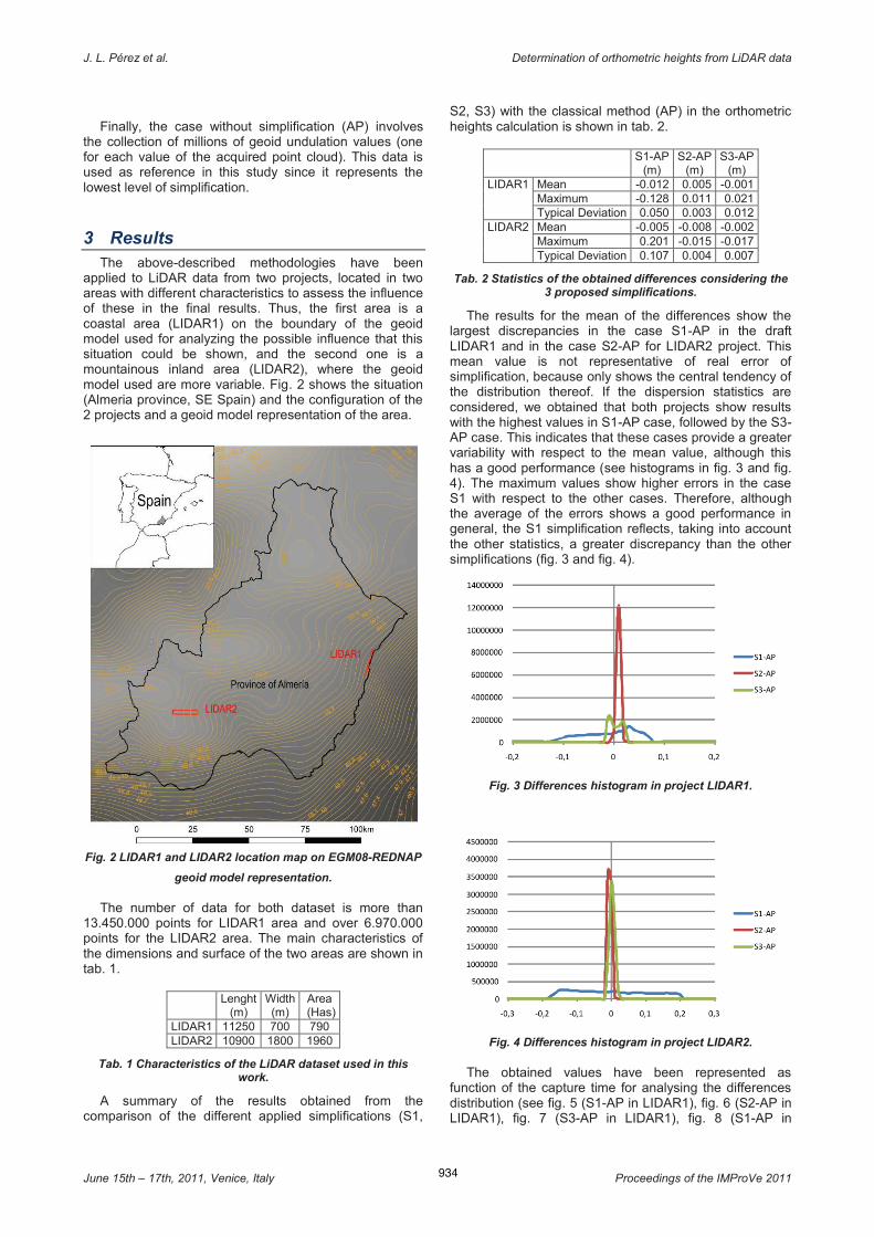
applied to LiDAR data from two projects, located in two areas with different characteristics to assess the influence of these in the final results. Thus, the first area is a coastal area (LIDAR1) on the boundary of the geoid model used for analyzing the possible influence that this situation could be shown, and the second one is a mountainous inland area (LIDAR2), where the geoid model used are more variable. Fig. 2 shows the situation (Almeria province, SE Spain) and the configuration of the 2 projects and a geoid model representation of the area.

Fig. 2 LIDAR1 and LIDAR2 location map on EGM08-REDNAP

geoid model representation.

The number of data for both dataset is more than 13.450.000 points for LIDAR1 area and over 6.970.000 points for the LIDAR2 area. The main characteristics of the dimensions and surface of the two areas are shown in tab. 1.

Lenght

(m) Width (m)

Area (Has)

LIDAR1 11250 700 790 LIDAR2 10900 1800 1960

Tab. 1 Characteristics of the LiDAR dataset used in this work.

A summary of the results obtained from the comparison of the different applied simplifications (S1,

S2, S3) with the classical method (AP) in the orthometric heights calculation is shown in tab. 2.

S1-AP

(m) S2-AP

(m) S3-AP

(m) LIDAR1 Mean -0.012 0.005 -0.001

Maximum -0.128 0.011 0.021 Typical Deviation 0.050 0.003 0.012

LIDAR2 Mean -0.005 -0.008 -0.002 Maximum 0.201 -0.015 -0.017 Typical Deviation 0.107 0.004 0.007

Tab. 2 Statistics of the obtained differences considering the 3 proposed simplifications.

The results for the mean of the differences show the largest discrepancies in the case S1-AP in the draft LIDAR1 and in the case S2-AP for LIDAR2 project. This mean value is not representative of real error of simplification, because only shows the central tendency of the distribution thereof. If the dispersion statistics are considered, we obtained that both projects show results with the highest values in S1-AP case, followed by the S3-AP case. This indicates that these cases provide a greater variability with respect to the mean value, although this has a good performance (see histograms in fig. 3 and fig. 4). The maximum values show higher errors in the case S1 with respect to the other cases. Therefore, although the average of the errors shows a good performance in general, the S1 simplification reflects, taking into account the other statistics, a greater discrepancy than the other simplifications (fig. 3 and fig. 4).

Fig. 3 Differences histogram in project LIDAR1.

Fig. 4 Differences histogram in project LIDAR2.

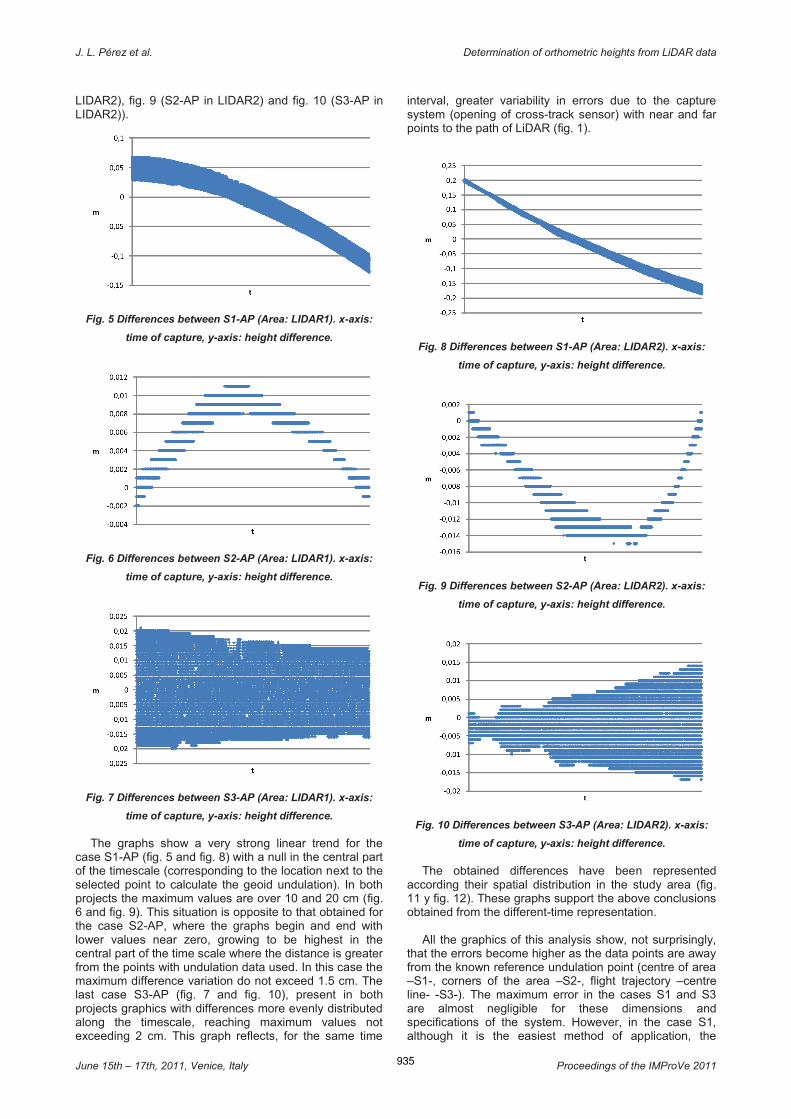
The obtained values have been represented as function of the capture time for analysing the differences distribution (see fig. 5 (S1-AP in LIDAR1), fig. 6 (S2-AP in LIDAR1), fig. 7 (S3-AP in LIDAR1), fig. 8 (S1-AP in

935



LIDAR2), fig. 9 (S2-AP in LIDAR2) and fig. 10 (S3-AP in LIDAR2)).

Fig. 5 Differences between S1-AP (Area: LIDAR1). x-axis:

time of capture, y-axis: height difference.





The graphs show a very strong linear trend for the case S1-AP (fig. 5 and fig. 8) with a null in the central part of the timescale (corresponding to the location next to the selected point to calculate the geoid undulation). In both projects the maximum values are over 10 and 20 cm (fig. 6 and fig. 9). This situation is opposite to that obtained for the case S2-AP, where the graphs begin and end with lower values near zero, growing to be highest in the central part of the time scale where the distance is greater from the points with undulation data used. In this case the maximum difference variation do not exceed 1.5 cm. The last case S3-AP (fig. 7 and fig. 10), present in both projects graphics with differences more evenly distributed along the timescale, reaching maximum values not exceeding 2 cm. This graph reflects, for the same time

interval, greater variability in errors due to the capture system (opening of cross-track sensor) with near and far points to the path of LiDAR (fig. 1).







The obtained differences have been represented according their spatial distribution in the study area (fig. 11 y fig. 12). These graphs support the above conclusions obtained from the different-time representation.

All the graphics of this analysis show, not surprisingly,

that the errors become higher as the data points are away from the known reference undulation point (centre of area –S1-, corners of the area –S2-, flight trajectory –centre line- -S3-). The maximum error in the cases S1 and S3 are almost negligible for these dimensions and specifications of the system. However, in the case S1, although it is the easiest method of application, the

936



observed maximum errors are not negligible taking into account the expected accuracies for the LiDAR system.

Fig. 11 Difference results in LIDAR1 area. Left: S1-AP;

Middle: S2-AP; Right: S3-AP.

Fig. 12 Difference results in LIDAR2 area: Upper: S1-AP ;

Middle: S2-AP; Bottom: S3-AP.

The analysis of the results must be made in accordance with the objectives of this work, i.e., determining which simplification (S1, S2, S3) is more adequate. According to the obtained differences distributions, S2 simplification shows lower values in the differences. Option S3 shows differences somewhat higher, especially in remote areas of the flight line. Finally, the case S1 is the one with greatest differences.

There is no significant difference between the two

considered areas (LIDAR1 and LIDAR2), appearing only differences due to the situation and geoid variation for each case (fig. 2).

On the other hand, we must take into account the

implementation effort of the options previously discussed. Jointly, the differences suggest the use of simplifications S1 and S2, which require less computational effort.

Ultimately, the choice of simplification must consider

several aspects:

- Absolute accuracy of orthometric height required in the project: based on this value will be eligible for option S1, when the accuracy is not very demanding or otherwise S2 option.

- Size of the area: In small areas, the S1 solution may be the most appropriate as it will greatly reduce the error, being the easiest option to implement.

- Variability and accuracy of the geoid model in the area: If there is not a very precise geoid model or low variability may also choose the option S1.

- In the case of working in large areas, with several flight lines, if the height transformation by blocks or lines is needed, it is necessary to applied a method that guarantees the geometrical continuity in overlap areas in order to obtain a continuous dataset that is an essential requirement for further processing of such data [11] [12]. In this case, and assuming some of the simplifications used here raised, the S2 is the option recommended because errors decrease to extremes, while in the options S3 and S1 these differences grow until the limits.

Finally, it is important take into account that the actual accuracy of the LiDAR system is around 15 cm. This means that all (or nearly all) the options considered in this paper generate differences around or below this value, so that all options used independently and with similar areas analyzed in this work could be viable in a similar context.

4 Conclusion The obtained results of this study show different error

patterns depending on the type of simplification used, which can establish an error model for each case. From this analysis we establish the values and distribution of errors in each simplification recommending setting the situation depending on the altimetric accuracy needed for the project, the size of the area and the variability and accuracy of the geoid model used.

The project characteristics must be the main aspect to

consider in order to select the type of simplification to be implemented, and currently the differences do not exceed the accuracy of the LiDAR system itself. In this regard, this study can be used in the future when the precision of this technique improved, to determine whether the simplification used in each case is consistent with the requirements of precision required.

Acknowledgement The authors are very grateful to Andalusia Regional

Government, Spain, for financing this work through the Excellence Research Project RNM-3575 “Multisource geospatial data integration and mining for the monitoring and modelling of coastal areas evolution and vulnerability. Application to a pilot area located at Levante de Almería, Spain”, and also through the project "Software for developping virtual digital space for its application to videogames and another interactive activities from real topological data obtained through digital sensor (LiDAR and digital camera)”. Avanza Programme (Subprogramme Avanza Competitivity R+D+i 2010) of the Spanish Ministry of Industry, Turism and Commerce, with partial funds of FEDER (European Union).

937



References [1] BOE: Boletín Oficial del Estado de España. Real Decreto 1071/2007, de 27 de julio, por el que se regula el sistema geodésico de referencia oficial en España. Boletín Oficial del Estado. 2007. http://www.boe.es/boe/dias/2007/08/29/pdfs/A35986-35989.pdf accessed 28 Jan 2011. [2] W. Torge. Geodesy. Ed. Walter de Gruyter. 2001. [3] Instituto Geográfico Nacional de España IGN. El nuevo modelo de geoide para España EGM08 – REDNAP. 2009. ftp://ftp.geodesia.ign.es/documentos/EL%20NUEVO%20MODELO%20DE%20GEOIDE%20PARA%20ESPA_A%20EGM08-REDNAP.pdf accessed 28 Jan 2011. [4] S.L. Smith, D. A. Holland, P.A Longley. The effect of changing grid in the creation of laser scanner digital surface models. Proceedings of the 7th International Conference on GeoComputation, September 8 th – 10th, 2003, University of Southampton (UK), pp 1-15. http://www.geocomputation.org/2003/Papers/Smith_Paper.pdf accessed 3 Feb 2011. [5] Leica ALS60 Airborne Laser Scanner Product Specifications. 2008. http://www.leica-geosystems.com/downloads123/zz/airborne/als60/product-specification/ALS60_ProductSpecs_en.pdf accessed 4 Feb 2011. [6] S. E. Reutebuch, R. J. McGaughey, H.-E. Andersen, W. W. Carson. Accuracy of a high-resolution lidar terrain model under a conifer forest canopy. Canadian Journal of Remote Sensing 29, 5 (2003), pp. 527–535. [7] M. E. Hodgson and P. Bresnahan. Accuracy of Airborne Lidar-Derived Elevation: Empirical Assessment and Error Budget. Photogrammetric Engineering & Remote Sensing 70, 3 (2004), pp. 331–339. [8] F. J. Aguilar and J. P. Mills. Accuracy assessment of LIDAR-derived Digital Elevation Models. The Photogrammetric Record 23, 122 (2008), pp. 148–169. [9] X. Liu. Accuracy assessment of lidar elevation data using survey marks. Survey Review 43, 319 (2011), pp. 80-93. [10] M. Flood. ASPRS guidelines. Vertical accuracy reporting for lidar data (2004). http://www.asprs.org/society/committees/standards/Vertical_Accuracy_Reporting_for_Lidar_Data.pdf accessed 4 Feb 2011. [11] J. Shan, C. K. Toth. Topographic laser ranging and scanning. Principles and Processing. CRC Press. 2009. [12] G. Vosselman, H-G. Maas. Airborne and terrestrial laser scanning. Ed. Whittles. 2010.

Documents

Determination of orthometric heights from LiDAR data · J. L. Pérez et al. Determination of orthometric heights from LiDAR dat a June 15th 17th, 2011, Venice, Italy Proceedings of