Embed Size (px)
Citation preview

1. R.porl ND. 2. Go".,,, ... ,,1 Acc.SSiDI'I ND.
FHWA/TX~82/34+256-2
... Titl. Dl'ld Sublill.
DETERMINATION OF IN SIro SHEAR WAVE VELOCITIES FROM SPECTRAL ANALYS IS OF SURFACE WAVES
,. A.,rho,'.)
J. Scott Heisey, Kenneth H. StoKoe, W. Ronald Hudson, and A. H. Meyer 9. P.r'orl'l\;"11 O'II01'1il.Gliol'l N_. OI'Id Add, ...
Center for Transportation Research
TECHNICAL REPORT STANDARD TITLE PAGE
3. R.ciP'.I'II'. CDIDlolI No.
5. R.po,' 0411.
December 1982
•• P.r'otl'''''11 O'IIGl'liI.DI;O" R.porl No.
Research Report 256-2
10. Work Unit No.
11. COI'II,oCI Of Gront No. The University of Texas at Austin Research Study 3-8-80-256 Austin, Texas 78712-1075
1-:'-:--::---______ ~~_--------------___l13, Type 0' RepDr' OI'Id P.riod Co ... r.d 12. SponaDril'l1l AII."cy N_. _., A.,d, ...
Texas State Department of Highways and Public Transportation; Transportation Planning Division
p. O. Box 5051 Austin, Texas 78763 15. S .. ppl ..... I'I'ory No'u
Interim
I... Sponaor;ng AII.l'lcy Cod.
Study conducted in cooperation with the U. S. Department of Transportation Federal Highway Administration
Research Study Title: "The Study of New Technologies for Pavement Evaluation" 16. Abs'racl
A method for determining elastic moduli at soil and pavement sites was proposed and tested. Surface receivers were utilized to evaluate the Rayleigh wave motion created by a vertical, impulsive source that could excite a wide range of frequencies with a single impact. Analysis was facilitated by using a portable spectral analyzer to study the magnitude and phase of the frequency content of the recorded wave pulse.
Results from field testing at two flexible pavement sites and two soil sites indicate that the spectral analysis of surface waves provides an accurate estimation of the velocity (and hence modulus) profile at a site. Moduli calculated from wave propagation velocities Were generally comparable to moduli calculated by deflection measurements from Dynaflect testing.
pavement evaluation, elastic modulus, nondestructive testing, seismic waves
II. Di • .,I .... '_ "et __ • No restrictions. This document is available to the public through the National Technical Information Service, Springfield, Virginia 22161.
19. Security CI ... ". (.f thi. ,.,.,.,
Unclassified
a. 5Murlty CI ... I'. Cof thl. , ... ,
Unclassified
21. N ••• f p.... 22. Price
292
Form DOT F 1700.7 '1.1t)

DETERMINATION OF IN SITU SHEAR WAVE VELOCITIES FROM SPECTRAL ANALYSIS OF SURFACE WAVES
by
J. Scott Heisey Kenneth H. Stokoe W. Ronald Hudson
A. H. Meyer
Research Report Number .256-2
The Study of New Technologies for Pavement Evaluation Research Project 3-8-80-256
conducted for
Texas State Department of Highways and Public Transportation
in cooperation with the U. S. Department of Transportation
Federal Highway Administration
by the
CENTER FOR TRANSPOR~TION RESEARCH BUREAU OF ENGINEERING RESEARCH
THE UNIVERS ITY OF TEXAS AT AUS TIN
December 1982

The contents of this report reflect the views of the authors, who are
responsible for the facts and the accuracy of the data presented herein. The
contents do not neceBsarily reflect the official views or policies of the
Federal Highway Adainistration. This report does not constitute a standard,
specification, or regulation.
ii

PREFACE
This report summarizes the results to date of an experimental study to
evaluate the use of spectral analysis of wave forces a a nondestructive
method of determining elastic moduli of pavement layers.
The project is being conducted at the Center for Transportation
Research, The University of Texas at Austin, as part of the Cooperative
Highway Research Program sponsored by the Texas State Department of Highways
and Public Transportation and the Federal Highway Administration.
Special appreciation is due Richard Rogers, Rarett Rakins, Jim Long, and
Leon Snyder for their assistaace concerning this project.
iii
J. Scott Heisey
Kenneth H. Stokoe, II
w. Ronald Hudson
A. H. Meyer

LIST OF REPORTS
Report No. 256-1, "Comparison of the Falling Weight Def1ectometer and the Dynaflect for Pavement Evaluation," by Bary Eagleson, Scott Heisey, W. Ronald Hudson, Alvin H. Meyer, and Kenneth H. Stokoe, presents the results of an analytical study undertaken to determine the best model for pavement evaluation using the criteria of cost, operational characteristics, and suitability.
Report No. 256-2, "Determination of In Situ Shear Wave Velocities From Spectral Analysis of Surface Waves," by J. Scott Heisey, Kenneth H. Stokoe II, W. Ronald Hudson, and A. H. Meyer, presents a method for determining elastic moduli at soil and paveMent sites. Criteria considered in developing this method included the restraint of nondestructive testing, accuracy of moduli for all layers regardless of thickness, and quickness and effeciency for rapid, extensive testing.
v


ABSTRACT
A method for determining elastic moduli at soil and pavement sites was
proposed and tested. Surface receivers were utilized to evaluate the
Rayleigh wave motion created by a vertical, impulsive source that could
excite a wide range of frequencies with a single impact. Analysis was
facilitated by using a portable spectral analyzer to study the magnitude and
phase of the frequency content of the recorded wave pulse.
Results from field testing at two flexible pavement sites and two soil
sites indicate that the spectral analysis of surface waves provides an
accurate estimation of the velocity (and hence modulus) profile at a site.
Moduli calculated from wave propagation velocities were generally comparable
to moduli calculated by deflection measurements from Dynaflect testing.
KEYWORDS: Pavement evaluation, elastic modulus, nondestructive testing,
seismic waves.
vii

J .
SUMMARY
A method for determining elastic moduli at soil and pavement sites was
proposed and tested. Criteria considered in developing this method included
the restraint of nondestructive testing, accuracy of moduli for all layers
regardless of thicknesses, and quickness and efficiency for rapid, extensive
testing. To meet these criteria, surface receivers were utilized to evaluate
the Rayleigh wave motion created by a vertical, impulsive source that could
excite a wide range of frequencies with a single impact. Analysis was
facilitated by using a portable spectral analyzer to study the magnitude and
phase of the frequency content of the recorded wave pulse.
Phase information from the cross spectrum function was used to calculate
Rayleigh wave velocities from which shear wave velocities were calculated.
Elastic moduli (shear moduli and Young's moduli) were then calculated from
the shear wave velocities. Results from field testing at two pavement sites
and two soil sites indicate that the spectral analysis of surface waves
provides an accurate estimation of the velocity (and hence modulus) profile
at a site.
comparable
testing.
Moduli calculated from wave propagation velocities were generally
to moduli calculated by deflection measurements from Dynaflect
ix

IMPLEMENTATION STATEMENT
The procedure described in this report should not be implemented at the
present time. The equipment and procedures are not sufficiently refined, and
the data are not adequate to establish standard tests.
xi


TABLE OF CONTENTS
PREFACE . . . . . . . . . . . . . . . . . . . . . . . . . . . . . . .
LIST OF REPORTS
ABSTRACT
SUMMARY
IMPLEMENTATION STATEMENT . . . . . . . . . . . . . . . . . . . . . . . CHAPTER 1. INTRODUCTION
CHAPTER 2. MEASUREMENT OF ELASTIC PROPERTIES BY WAVE PROPAGATION
Review of Wave Propagation Theory • • . • Wave Propagation in an Elastic Half-Space • • • •
Wave Propagation in a Layered System Field Techniques for Determining Elastic Properties
Investigation of Soil Profiles . . . • . Evaluation of Pavements
Application of Spectral Analysis . •
CHAPTER 3. DIGITAL SIGNAL AND SPECTRAL ANALYSES
Time Domain Measurements Averaging •••• Correlation
. . . . . . . . . . . . .
Frequency Domain Measurements Advantages of Spectral Analysis
. . . t • • • • • • • • • • •
The Fourier Transform ••••••••. Measurements in the Frequency Domain
Linear Spectrum • • Auto Spectrum Cross Spectrum Transfer Function Coherence Function
Additional Considerations for Digital Signal AnalYSis • • •
xiii
iii
v
vii
ix
xi
1
5 5
13 15 15 22 25
29 29 30 33 33 36 40 40 40 41 42 42 44

xiv
CHAPTER 4. SOIL TESTING AT WALNUT CREEK SITE
Site Description Experimental Procegure
Test Series WC-l Test Series WC-2 Recording of Spectral Measurements
Description of Sources • • • . • • Drop HanJIDer . • • • • • • • • • • • Drop Hammer on Embedded Steel Wedge • . • • • Sledge Hammer on Embedded Concrete Cylinder • Small Hammer on Wooden Plate • • • •
Comparison of Significant Parameters Number of Averages Measurement Bandwidth • Sources • • • • • • •
Test Series WC-l • Test Series WC-2 .
Spatial Distribution of Shear Wave Velocity Profile
Crosshole Test Results
Geophones
Velocity Profile from Cross Spectrum Measurements . Comparisons Between Cross Spectrum Measurements and Crosshole Results • • . . • •
Attenuation Measurements Summary .. • . • • • .
CHAPTER 5. SOIL TESTING AT THE CROSSING SITE
Site Description ..... Experimental Procedure Shear Wave Velocity Profile
Velocity Profiles From Cross Spectrum Measurements Comparison Between Cross Spectrum Measurements and Crosshole Results •••.
Attenuation Summary
CHAPTER 6. PAVEMENT EVALUATION AT AUSTIN SITE
Site Description • • • •
. . . . .
Experimental Procedure • • • • • • • • . • . • • Equipment . . . t • • • • • • • • • • • • •
Measurement Setup and Analysis •••••.•.••••.••
47 47 50 52 59 60 60 61 61 63 63 63 66 74 74 76 84 96 96 99
101 105 116
119 121 123 126
134 138 148
151 154 154 156
Results from Surface Measurements . . . . . . . . . Comparison of Horizontal and Vertical Geophones Analysis of the Falling Weight Deflectometer Analysis of the Drop Hammer ...•... Comparison of the FWD and the Drop Hammer
Results from Crosshole Testing Description of Test Procedure . Analysis of Crosshole Data
Determination of Moduli Summary
CHAPTER 7. PAVEMENT EVALUATION OF GRANGER SITE
Site Description .•..•...• Experimental Procedure • • • . . . Determination of Velocity Profile Determination of Moduli SUIIIdlary • • • • • • • '. • • • • • •
. .
CHAPTER 8. SUMMARY, CONCLUSIONS, AND RECOMMENDATIONS
Summary . . . . . . . . . . . . . . . . . . . . . . . . . General Conclusions Regarding Test-Related Variables . Conclusions and Recommendations for Soil Investigation Conclusions and Recommendations for Pavement Evaluation
REFERENCES . . . . . . . . . . . . . . . . . . . . . . . . . . . . . .
APPENDICIES
Appendix A. Discussion of Experimental Procedures and Data Analysis . . • . . . .
Appendix B. Computer Programs and Plot Routines
THE AUTHORS . . . . . . . . . . . . . . . . . . . . . . . . . . . . .
xv
158 160 166 172 178 184 184 186 193 194
197 200 202 216 218
221 222 224 226
229
235
255
275
CHAPTER l. INTRODUCTION
Wave propagation velocities are used to determine material properties
which characterize the response of systems undergoing low-strain, dynamic
loading. Examples of such systems are foundations which support vibrating
machinery and pavements which support repetitive traffic loads. In the
dynamic design of foundations, material properties are generally
characterized by the shear modulus. For the design of pavement systems,
material properties are characterized by the elastic (Young's) modulus. Both
moduli can be easily calculated if the shear wave velocities of the materials
of concern are known.
In this s~udy, a method was investigated to determine shear wave
velocities from the frequency spectrum of surface waves. Both the source of
surface wave energy and the receivers to detect wave motion are located on
the surface. This approach eliminates the need for drilling and coring. As
a result, the time and costs of a site investigation are greatly reduced.
The method is quick and nondestructive, thereby making it feasible for the
evaluation of existing pavement systems. In addition, the analysis of the
frequency spectrum of the surface wave(s) provides data for individual layers
in a multilayered system.
Basic theory of wave propagation pertinent to this method is briefly
reviewed in Chapter 2. Conventional techniques for site investigation and
pavement evaluation are also discussed. The spectral analysis method is
1

2
presented and discussed in relation to the theory and in comparison with
other methods. Chapter 3 introduces the reader to the theory and mathematics
of the Fourier transform, which provides the framework for spectral analysis.
Various functions derived from frequency spectrums are defined and their
general uses are described.
Field investigations were conducted at two sites where the profile
included a flexible pavement surface, a base course, and subgrade soil
(referred to as pavement sites) and at two sites where the profile included
only soil (referred to as soil sites). The soil sites were investigated to
determine the influence of the relatively stiff layers at the surface of a
pavement system on the propagation of surface waves through the underlying
soil. The soil sites which were selected had previously been investigated by
crosshole seismic testing and thereby provided additional test sites to
verify the applicability and accuracy of the spectral analysis method.
Results from the soil sites, Walnut Creek and the Crossing, are
presented in Chapters 4 and 5, respectively. Test-related variables which
were studied include type of source, number of averages in the measurement,
frequency range of the measurement bandwidth, location of the receivers from
the source, and the appropriate depth factor to correlate the measured
velocity profile with known field conditions.
Results from the pavement sites, IH 35 in Austin, Texas, and FM 971 near
Granger, Texas, are presented in Chapters 6 and 7, respectively. At the
Austin site, comparison measurements were made between the Falling Weight
Deflectometer and a small, hand-held drop hammer. Other test-related
variables included: orientation of the receivers (for horizontal or vertical
motion), location of the receivers from the source, and frequency range of
the measurement.

3
At all four sites, data from crosshole seismic testing either available
or were gathered for comparison purposes. Comparisons between the velocity
profiles obtained from crosshole testing and those obtained from spectral
analysis of surface waves indicate that, in general, the spectral analysis
method provides an accurate estimation of the velocity (and, hence, modulus)
profile of a site. However, further investigation of some of the
test-related variables is necessary to refine the method and to reinforce the
conclusions of this study. Conclusions and recommendations for future
research are summarized in Chapter 8.
For the benefit of the reader, a detailed discussion of the experimental
procedure and useful data reduction is presented in Appendix A. The computer
programs used for data reduction and analysis are listed in Appendix B.


CHAPTER 2. 100fEASUREMENT OF ELASTIC PROPERTIES BY WAVE PROPAGATION
REVIEW OF WAVE PROPAGATION THEORY
Since the stress-stratn properties of a material govern wave propagation
velocities in that material, dynamic (also called seismic) testing can be
used to determine wave propagation velocities from which moduli of the
material can be calculated. These moduli characterize behavior in the
"elastic" range, where the material is undergoing very small strains.
Relationships between moduli and wave propagation velocities are presented in
the following sections. A more complete and rigorous discussion on wave
propagation in elastic media can be found in the textbooks by Richart, Hall,
and Woods (1970) and Ewing, Jardetzky, and Press (1957).
WAVE PROPAGATION IN AN ELASTIC HALF-SPACE
Wave motion created by a disturbance within an infinite, isotopic,
elastic medium, usually called a ·whole space," can be described by two kinds
of waves: compression waves and shear waves. These waves are called body
waves because they propagate within the body of the medium. When the elastic
medium forms a half-space with an upper surface of infinite extent, a third
type of wave motion occurs. This third type of wave occurs in a zone near
5
• ~ ,
6
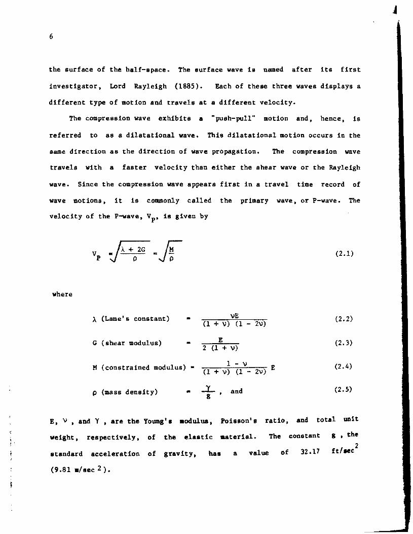
the surface of the half-space. The surface wave Is named after its first
investigator, Lord Rayleigh (1885). Each of these three waves displays a
different type of motion and travels at a different velocity.
The compression wave exhibits a "push-pull" motion and, hence, is
referred to as a dilatational wave. This dilatational motion occurs in the
same direction as the direction of wave propagation. The compression wave
travels with a faster velocity than either the shear wave or the Rayleigh
wave. Since the compression wave appears first in a travel time record of
wave motions, it is commonly called the primary wave, or P-wave. The
velocity of the P-wave, Vp ' is given by
where
A (Lame's constant) -G (shear modulus) -H (constrained modulus) -
p (mass density) •
vE (1 + v) (1 - 2v)
E 2 (1 + v)
1 - v (1 + v) (1 - 2v) E
..L g
and
(2.1)
(2.2)
(2.3)
(2.4)
(2.5)
E, v , and Y , are the Young's .odulU8, Poi880n's ratio, and total unit
weight, respectively, of
standard acceleration of
(9.81 ./sec 2).
the elastic asterial. The
gravity, has a value
constant
of 32.17
I , the
ft/Me2
J

7
The shear wave, also called a distortional wave, exhibits shearing
motion which is perpendicular to the direction of wave propagation. The
shear wave travels significantly slower than the P-wave and, as a result,
appears later in a travel time record. It is commonly called the secondary
wave, or S-wave, because it arrives after the P-wave. The velocity of the
S-wave, Vs ' is given by
(2.6)
Unlike P-waves, whose velocities can vary with the degree of saturation of a
porous medium, S-waves have essentially the same velocities in a saturated
medium as in an unsaturated medium because the fluid cannot transmit shearing
motion.
The Rayleigh wave, or R-wave, does not propagate into the body of the
elastic medium but travels along the surface of the half-space. The wave
motion causes both horizontal and vertical particle displacements, which
describe a retrograde ellipse at the surface. The amplitude of the wave
decays quickly with depth such that at a depth of one wavelength, the
amplitude of particle motion is only about 30 percent of the original
amplitude at the surface. The velocity of the R-wave, VR ' is nearly equal
to the S-wave velocity, particularly for values of Poisson's ratio above
0.40. In addition, R-wave velocity is independent of frequency in a
homogeneous half-space. Since an ideal elastic half-space has a unique
R-wave velocity, each frequency has a corresponding wavelength according to
the relationship
f • L R (2.7)

8
where f is the input frequency of excitation that generates a Rayleigh wave
of wavelength The frequency-independent nature of the R-wave is the
basis for certain types of dynamic testing.
The propagation of wave energy away from a vertically vibrating,
circular footing resting on the surface of an elastic half-space is shown in
Fig 2.1a. This figure illustrates the three types of waves just discussed.
Miller and Pursey (Ref 18) found that, for the vertically OSCillating,
circular, energy source shown in Fig 2.1a, 67 percent of the input energy
propagates away in the form of Rayleigh wave energy while 26 percent is
carried by the shear wave and 7 percent is carried by the compression wave.
Body waves, P- and S-waves, propagate radially outward along a hemi spherical
wave front, while the Rayleigh wave propagates radially outward along a
cylindrical wave front at the surface.
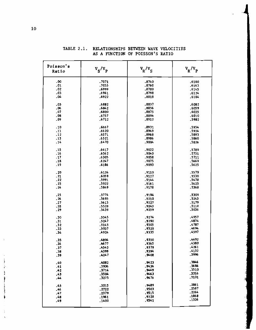
The propagation velocities of all of these waves relative to the shear
wave velocity are shown as a function of Poisson's ratio in Fig 2.1b. For
the range of Poisson's ratio of most 80ils and pavement materials
(0.25 ~ V 20.45), VR is generally approximated as 0.95 VS. The exact
relationships between Vp , VR ' and Vs over the entire range of Poisson's
ratios are listed in Table 2.1.
It should be noted that
propagation velocities of
velocities of the medium
the velocities Vp , VR ' and V S are the
the respective wave fronts. and not the R!rticle
itself due to the wave energy. Figure 2.2
illustrates the particle .otion caused by the various waves propagating in an
elastic half-8pace.
As wave fronts propagate away from a source, they encounter a greater
volume of the half-space, which caU8es the wave energy to dissipate with
distance from the source. This phenomenon is referred to as geometrical

(a) Distribution of waves from a vertically vibrating footing on a homogeneous, isotropic, elastic halfspace (Ref 23).
s-Wo,,"
'======~=====------1 R-Woves
o Poisson', Rotio. to
(b) Relationship between Poisson's ratio and wave velocities in an elastic half-space (Ref 23).
Fig 2.1. Propagation of waves in an elastic half-space.
9
10
TABLE 2.1. RELATIONSHIPS BETWEEN WAVE VELOCITIES AS A FUNCTION OF POISSON'S RATIO
Poisson's VS!Vp VR!VS VR!VP Ratio
.00 .7071 .8740 .6180
.01 .7035 .8760 .6163
.02 .6999 .8780 .6145
.03 .6961 .8798 .6124
.04 .6922 .8818 .6104
.05 .6882 .8837 .6082
.06 .6842 .8856 .6059
.07 .6800 .8875 .6035
.08 .6757 .8894 .6010
.09 .6712 .8912 .5982
.10 .6667 .8931 .5954
.11 .6620 .8949 .5924
.12 .6571 .8968 .5893
.13 .6521 .8986 .5860
.14 .6470 .9004 .5826
.15 .6417 .9022 .5789
.16 .6362 .9040 .5751
.17 .6305 .9058 .5711
.18 .6247 .9075 .5669
.19 .6186 .9093 .5625
.20 .6124 .9110 .5579
.21 .6059 .9127 .5530
.22 .5991 .9144 .5478
.23 .5922 .9161 .5425
.24 .5849 .9178 .5368
.25 .5774 .9194 .5309
.26 .5695 .9210 .5245
.27 .5613 .9227 .5179
.28 .5528 .9243 .5110
.29 .5439 .9259 .5036
.30 .5345 .9274 .4957
.31 .5247 .9290 .4874
.32 .5145 .9305 .4787
.33 .5037 .9320 .4694
.34 .4924 .9335 .4597
.35 .4804 .9350 .4492
.36 .4677 .9365 .4380
.37 .4543 .9379 .4261
.38 .4399 .9394 .4132
.39 .4247 .9408 .3996
.40 .4082 .9423 .3846
.41 .3906 .9436 .3686
.42 .3714 .9449 .3510
.43 .3504 .9463 .3n6
.44 .3273 .9476 .3101
.45 .3015 .9489 .2861
.46 .2722 .9503 .2587
.47 .2379 .9515 .2264
.48 .1961 .9528 .1868
.49 .1400 .9541 .1336

f
(b) 5_
(c) Lowe ....
~
(d)
, t
t ,
, ,
Fig 2.2. Forms of wave motion in an elastic half-space (Ref 4).
11

12
damping or geometrical attenuation. The relationships governing geometrical
damping of wave energy as a function of distance from the source (r) are
shown in Fig 2.la. At the surface, the amplitudes of P- and S-waves decrease
as l/r2, whereas the R-wave amplitude decreases only as l/~ • As a
result, in a relatively short distance from the source, most of the energy
(at the surface) is R-wave energy.
Besides geometrical damping, material damping causes energy dissipation
since soil and rock are not perfectly elastic. Material damping can be
expressed in terms of a coefficient of attenuation, which is related to
R-wave attenuation as follows
where
(2.8)
Al - amplitude of the vertical component of the R-wave at a distance
r 1 from the source,
A2 - amplitude of the vertical component of the R-wave at a distance
r 2 from the 80urce, and
a - coefficient of attenuation, with diaensions of l/distance and the
same units as r l and r 2 •
Material damping can also be expres8ed. in terms of the logarithmic decrement
o which is related to a as follows
o - a· (2.9)
J

13
Damping is most often expressed in terms of a damping ratio D, which is
related to 6 as follows
D = (2.10)
Material damping (D or 6 ) in earth materials is usually assumed to be
independent of frequency. Therefore, the coefficient of attenuation a must
be a function of frequency. McDonal, et a1 (Ref 17» and Kudo and Shima
(Ref 14) showed to be a linear function of frequency. Szendrei and
Freeme (Ref 26) detected different values of a corresponding to individual
layers in a pavement system.
Wave Propagation in a Layered System
The previous section dealt with body and surface waves in an elastic
half-space. However, in the case of a pavement section, these waves
propagate through a layered system, which complicates the problem. When body
waves reach an interface between two layers, some of the body wave energy is
reflected back into the first layer and some is transmitted by refraction
into the second layer. The combination of reflected and refracted body waves
from a layered system greatly increases the complexity in analyzing wave
arrivals.
In a horizontally layered system, an initial complication occurs because
the incident shear wave may actually be composed of two components, SV-waves
and SH-waves. The SV-wave propagates in a plane perpendicular to the plane
of the interface, while the SH-wave propagates in a plane parallel to the

I
14
interface. An incident SV-wave creates reflected P- and SV-waves and
refracted P- and SV-waves. In addition to the shear waves, each incident
P-wave results in a reflected P-wave, a refracted P-wave, a reflected
SV-wave, and a refracted SV-wave. In just a horizontal, two-layered system,
three incident body waves have generated ten new waves.
The redistribution of body wave energy is influenced by three variables
(1) the angle of incidence of the incident wave,
(2) the ratio of wave velocities in the two media, and
(3) the ratio of densities in the two media.
Therefore, the redistribution of wave energy becomes quite complicated in a
simple two-layered system. Wave detection becomes even more difficult in
multi-layered systems.
Special cases of reflected and refracted body waves may also occur.
Wben a reflected SH-wave in the upper layer reaches the surface, it will be
totally reflected. Multiple total reflections of SH-waves from the layer
interface can generate another type of surface wave, a Love wave. Love waves
are horizontally polarized shear waves confined to a surface layer. Such a
wave cannot occur if the upper layer has a higher velocity than the lower
layer. Love waves travel at a velocity which is between the shear wave
velocities of the two layers and i. dependent on the wavelength.
In addition, surface waves can be complicated in a layered system.
First, depending on the frequency of excitation and material properties at a
given aite, higher order .odes of Rayleigh wave vibration may occur. Second,
waves can exi8t at the boundaries between layers; they are 5toneley (Ref 25)
waves. These waves are analogous to Rayleigh waves in that they occur at tbe
interface of two materials and travel at a velocity approximately equal to
15
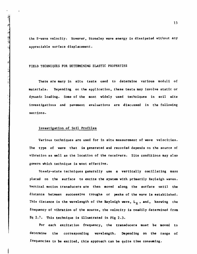
the S-wave velocity. However, Stoneley wave energy is dissipated without any
appreciable surface displacement.
FIELD TECHNIQUES FOR DETERMINING ELASTIC PROPERTIES
There are many in situ tests used to determine various moduli of
materials. Depending on the application, these tests may involve static or
dynamic loading. Some of the most widely used techniques in soil site
investigations and pavement evaluations are discussed in the following
sections.
Investigation of Soil Profiles
Various techniques are used for in situ measurement of wave velocities.
The type of wave that is generated and recorded depends on the source of
vibration as well as the location of the receivers. Site conditions may also
govern which technique is most effective.
Steady-state techniques generally use a vertically oscillating mass
placed on the surface to excite the system with prbDarily Rayleigh waves.
Vertical motion transducers are then moved along the surface until the
distance between successive troughs or peaks of the wave is established.
This distance is the wavelength of the Rayleigh wave, LR ,and, knowing the
frequency of vibration of the source, the velocity is readily determined from
Eq 2.7. This technique is illustrsted in Fig 2.3.
For each excitation frequency, the transducers must be moved to
determine the corresponding wavelength. Depending on the range of
frequencies to be excited, this approach can be quite time consuming.

16
• i. f
f
~: I
Source Vibrating at Frequency f
Direction of Propagation -----...........
Vertical Receiver
vR = f LR
vI
(a) Measurement of steady-state, Rayleigh - wave motion.
>u r:: •
100
80
80
; 40
• ... '"
20
o
o
/
/ /
/
200 «lO eoo VelOCity. fps
(b) Typical results.
800
Fig 2.3. Steady-state, Rayleigh-wave testing in layered systems.

17
Since most of the Rayleigh wave energy travels through a zone within
about one wavelength of the surface, the velocity of the Rayleigh wave is
influenced primarily by material properties to a depth of one wavelength.
When the steady-state technique shown in Fig 2.3 is used at a given site, low
frequencies generate long wavelengths corresponding to deep "sampling" of the
site. Conversely, high frequencies generate short wavelengths corresponding
to shallow sampling. In an ideal, homogeneous, elastic half-space, the
material properties do not change with depth. Therefore, the Rayleigh wave
velocity is independent of frequency (or wavelength). However, if the
properties vary with depth, the Rayleigh wave will become dispersed, i.e.,
different frequencies will travel at different velocities. As such,
different wavelengths will be sampling different elastic properties.
It is apparent that a given wavelength will sample the average
properties within about one wavelength of the surface. (In addition, lateral
variation in soil properties will be averaged over the distance of the
particular measurement.) It is not clear, however, at what depth the measured
velocity (or modulus) should be assigned. As a first approximation, this
depth could be taken as one-half the wavelength (L R /2). assuming that the
average properties are equally weighted over the full wavelength. Fry
(Ref 7), Ballard (Ref 1), and Ballard and Casagrande (Ref 2) reported field
tests that showed good correlation between measured wave velocities plotted
at a depth of L /2 and the soil profile at the test site. R
However, the displacement amplitude (and, hence, wave energy) is not
equally distributed over the full wavelength, as indicated by the curves
shown in Fig 2.4. For the vertical component of wave motion, the wave energy
is more concentrated toward the surface. As can be seen in Fig 2.4, the
amplitude function W(z) varies slightly with the Poisson's ratio of the

18
I
I ,
-0.6 -0.4
An!C)Ii1ude at DIpth 1
Amplitude of Swface 0.2 0.4 0.6 0.8 o
[ ~ 0.6 """""""1
W(I)J ... .J ........... 0.8 £ r
0.-
1.0 ~ j
1.2
1.4
Fig 2.4. Variation of Rayleigh-wave amplitude as a function of depth normalized to wavelength (Ref 23).

19
material. For the range of Poisson's ratios of most earth materials, the
"centroid" of wave energy distribution is located at a depth approximately
equal to LR /3, suggesting that measured wave velocities may more nearly
correspond to properties at a depth of one-third of the wavelength rather
than one-half of the wavelength.
Using the L R /3 criterion, the data presented by Fry (Ref 7) for the
Eglin Field test site were reexamined. Figure 2.5 shows a comparison of the
measured Rayleigh-wave velocity profile (using both L R /2 and L R /3 as
criteria for depth) with the theoretical variation of Rayleigh-wave velocity
with depth. The theoretical curve for the Eglin Field site was determined by
Richart, Hall, and Woods (Ref 23). They calculated shear wave velocities as
a function of depth based on an empirical relationship incorporating void
ratio (e = 0.70) and effective confining pressure (cr ) as a function of o
depth. Shear wave velocities were converted to Rayleigh wave velocities
using the relationship of VR = 0.933 Vs for \) - 1/3. Figure 2.5
indicates that the measured velocities, when plotted at a depth of L R /3,
correlate better with the theoretical curve than when plotted at a depth of
Other surface measurement techniques utilize an impulsive source.
Several types of surface techniques are shown in Fig 2.6. Usually,
velocities of P-waves are determined in these surveys. Travel times and
travel distances to the receiver may be determined for the direct arrival or
for an initial reflection in the upper layer. However, refracted waves are
normally encountered and care must be taken not to identify refracted waves
as direct waves. To overcome this problem, refraction surveys are performed
which take advantage of the faster-travelling refracted waves to develop the
profile and corresponding velocities for a layered system. Such an analysis

20
2
4
- 6 CI) CI) -. ~
- 8 Q. CI)
Cl
10
12
14
o
o LR/2 (After Fry)
o LR/3 (By Authors)
_ Theoretica I Curve (From Richart, Hall, and 'Abods , 1970)
200 400 Velocity, fps
o
600
Fig 2.5. Comparison of depth criteria using data frOD Eglin Field site (Ref 7).

t ----~Or_========~,~g~------
Layer I, vI
I J x\ \ Layer 2, v2 >v I
(a) Direct arrival survey.
Layer I, v I
Layer 2, v2 >v I
(b) Reflection survey.
Layer I, vI
Layer 2,v2 >vl
(c) Refraction survey.
Fig 2.6. Surface measurements based on arrival times of various body waves.
21

22
is greatly complicated for a site with many layers or dipping strata.
Refraction surveys are also hindered when a higher-velocity layer overlays a
lower-velocity layer, as in the case of a pavement surface overlaying a base
course or subgrade.
An alternative to surface measurement techniques is crosshole seismic
testing. This method is discussed in detail by Stokoe and Hoar (Ref 24).
The source and receivers are placed in drilled holes so that direct arrivals
of waves can be determined. Both P- and S-wave velocities are measured in
this type of test. Layering and velocities are accurately determined.
Proper spacing of the boreholes el~inates or min~izes problems caused by
refracted waves. A major drawback of the crosshole test is the high cost
associated with the drilling of several boreholes.
Downhole seismic testing utilizes an impulsive source at the surface and
requires only one borehole for placement of receivers. This method has been
investigated extensively by Patel (Ref 20).
velocities are determined from downhole testing.
In general, only S-wave
The necessity for boreholes
prevents use of both the downhole test and the crosshole test in normal
pavement evaluations.
Evaluation of Pavements
Lytton, Moore, and Mahoney (Ref 16), in a state-of-the-art report,
discuss four general methods used to evaluate elastic moduli of paveaent
systems: static deflections, steady-state dynamic deflections, impact load
response, and wave propagation methods. Each of these methods is briefly
summarized in the following paragraphs.
J.
23
Static deflection methods include the plate bearing test, curvature
meter, Benkelman beam, travelling deflectometer, and laCroix deflectograph.
Each of these methods measures pavement deflection under static loading.
Elastic layer theory is then used with the measurements to calculate moduli
indirectly on the basis of the measured deflections. In general, static
methods require some reference to establish a datum for the deflection
measurements.
Steady-state dynamic deflection methods measure deflections caused by
steady-state vibrations. Current equipment includes the Road Rater, the
Dynaflect device, and the WES Vibrator, among others. Moduli are then
calculated on the basis of the measured deflection basin using elastic layer
theory. The major drawback of the steady-state method is that the stiffness
of the entire pavement system is measured. Separation of the properties of
the individual layers is extremely difficult unless measurements are
performed at many different frequencies. This integrating effect also
prevents determination of the modulus of the relatively thin surface layer.
Impact load response methods involve monitoring the displacement-time
response, x(t), at the pavement surface due to a transient impulse force,
f(t). If the pavement is approximated as a single-degree-of-freedom
mechanical system with a mass, spring, and dashpot, the pavement stiffness is
an overall stiffness of the pavement system. Impact testing, however, does
offer the advantage of exciting a wide range of frequencies with just one
impulse. This type of excitation provides a quick and thorough technique for
extensive field testing.
Wave propagation methods measure the velocities of elastic waves
travelling through the pavement system, rather than the deflections caused by
the vibration source. Elastic waves can be generated by steady-state
24
vibrations or transient t.pulses, and they can propagate through individual
layers or the entire pavement system. Wave propagation methods, although not
widely used, offer the most direct approach to determining elastic moduli of
pavement systems.
Among wave propagation methods, the steady-state technique is most
widely used in nondestructive pavement testing. In multilayered systems, the
Rayleigh wave propagates at a velocity which reflects the material properties
of the layer{s) that the wavelength samples. Short wavelengths within the
surface layer will measure properties in that layer only. Long
(relative to the depth of the surface and base courses)
wavelengths
will travel
predominantly through the subgrade. Intermediate wavelengths will sample the
base course or average the properties of all three materials: surface, base,
and subgrade. Each wavelength will then have a corresponding phase velocity,
depending on how much of each layer the wave samples.
The mathematical analysis required to interpret the phase
velocity-wavelength relationship for several typical pavement sections was
studied by Jones (Ref 13). Jones assumed homogeneous, elastic layers while
treating the subgrade as a semi-infinite medium and showed that at infinitely
long wavelengths, the phase velocity approached the R-wave velocity of the
semi-infinite medium. S~ilarly, at very short wavelengths, the phase
velocity approached the R-wave velocity of the surface layer. Theoretical
solutions for an intermediate layer required more assumptions.
Although earth aaterials are neither perfectly homogeneous or elastic,
field investigations indicate that such assumptions are reasonable. Beukeloa
and Foster (Ref 8) reported a profile of velocity versus depth that sboved
good correlation with the paveaent profile when the effective sampling depth
was taken as one-half of the Rayleigh wavelength. Szendrei and lre .. e

25
(Ref 26) found a similar correlation by using an effecti~e sampling depth of
approximately
suggested that
one-third of the Rayleigh wavelength. Heukelom (Ref 8)
the sampling depth may vary from one-half to one-third the
Rayleigh wavelength, depending on the particular properties at a given site.
It should be emphasized that the use of any such depth criterion is primarily
empirical.
APPLICATION OF SPECTRAL ANALYSIS
Based on the preceeding review of results published in the literature,
it appears that the steady-state vibration technique is a valid means of
determining wave velocities and moduli of both
systems. Because individual layers can be
soil profiles and pavement
identified by contrasting
velocities, determination of moduli directly from wave propagation velocities
is more desirable than indirect calculation based on deflection measurements
and elastic layer theory. However, there are two drawbacks to the
conventional steady-state technique.
First, determination of wavelength requires measurement of the phase
difference between signals at two motion transducers. The conventional
approach was to move one transducer relative to the other until the signals
were .0 io phase, .. i.e. , the distance between transducers was an integral
mUltiple of the wavelength generated by the particular frequency. This
trial-and-error approach resulted in excessive time to complete the test.
With the advent of more sophisticated equipment, the phase difference between
sinusoidal waveforms could be identified regardless of the spacing between
transducers. Using such a phase computer in conjunction with steady-state

26
sources, Rao and Harnage (Ref 21) reported moderate success for vibration
tests on a rigid pavement test section and indicated that investigations
should be extended to actual field sites.
Secondly, the conventional steady-state technique uses a vertically
oscillating mass that excites only one frequency at a time. However, a wide
range of frequencies is required to generate the appropriate wavelengths
needed to sample a site. Again, this approach resulted in excessive time to
complete the test.
If the steady-state technique is modified to use an impulsive source to
propagate a transient wave pulse through the materials to be tested, a wide
range of frequencies can be excited at one time. This approach requires that
the time domain waveform be transformed into its frequency spectrum.
Spectral analysis instrumEntation is required to record, transform, and
analyze signals for their frequency and phase relationships. (M
introduction to the theory and mathematics involved in spectral analysis is
presented in Chapter 3.) The goal of this study was to implement such
instrumentation to develop a transient technique to determine a profile of
wave velocity (modulus) versus depth. The main advantage of the transient
technique is that it is significantly quicker and more "efficient than the
conventional steady-state technique.
In this study, various parameters were investigated to determine their
influence on the measurement of an accurate velocity profile. These
parameters included the number of averages (transient events) needed to
obtain a representative measurement, the appropriate frequency bandwidth(s)
to be analyzed, the type of source required to generate Rayleigh wave energy,
the appropriate location of the geophone nearer to the source, and the

27
appropriate spacing between geophones. In addition. the empirical depth
criteria (L R /2 and LR /3) were reexamined.
Data from surface measurements were also compared with data from
croBsho1e tests. No published data could be found in the literature where
results from the two techniques are compared. Previous comparisons were
based on other types of modulus tests. theoretical velocity profiles
calculated from laboratory soil properties and empirical relationships, or
solely on correlation between known layer boundaries and velocity contrasts
in different materials. The direct comparison of velocities obtained from
both surface measurements and crossho1e tests indicates that the spectral
analysis of surface waves is a valuable method for determining shear wave
velocities and elastic moduli.
«

· .
CHAPTER 3. DIGITAL SIGNAL AND SPECTRAL ANALYSES
TIME DOMAIN MEASUREMENTS
Conventional travel time methods usually employ a single-channel,
dual-channel, or multi-channel recorder to determine direct arrival or
interval travel times. Often it is difficult to detect sharp arrivals of the
various elastic waves in the waveform. Digital analysiS of time domain
measurements introduces two additional techniques to analyze poorly defined
signals: averaging and correlation.
Averaging
Averaging clarifies the signal by reinforcing the desired waveform and
by reducing background noise that obscures the Signal. A trigger is required
to synchronize the averaging of measurements. If the system input is
perfectly repeatable and the system in linear, then ideally the response for
each measurement will be identical. In the case of waves propagating through
elastic media, an input source that can be adequately reproduced does
reasonably duplicate the output waveform. Sufficient averaging causes any
slight variances to be "cleaned out" so the remaining signal approaches its
mean value. Since noise is essentially random ,it will average to a mean
29

30
value of zero. The benefit of averaging in signal recognition is shown in
Fig 3.1.
There are several types of averaging. Stable averaging weighs each
measurement equally, which is the conventional definit ion of .. average."
Exponential decay averaging weighs newer measurements more heavily than older
ones. Exponential decay averaging is useful for systems with behavior that
is changing with time while the measurements are being taken. Since the
behavior of a pavement system does not change with time (within the time
frame that measurements are made), stable averaging is the better technique.
Stable averaging of time domain measurements is referred to as time record
averaging.
Correlation
Two random variables that display a definite pattern or relationship are
said to be correlated. When a linear least-squares fit is performed, the
deviation of the data from the regression line is measured by the normalized
covariance or correlation coefficient, P • Data for which P equals unity xy xy
are perfectly correlated, while data for which Pxy equals
(linear) correlation.
zero contain no
Generally, correlation is associated with sets of discrete pairs of
data, but it is also applicable to continuous functions of time. A
collection of data is an ensemble of tiae records instead of discrete points.
The correlation function is actually a type of time average that measures the
similarity of two signals.

31
4.0
--
M ~II III
I~ -' '0-0>
.-I~- ~ as c y ~ 00-.... tf.l
--
-4.0 I I I I I I I I I
0 Time, seconds 1.0
(a) Single time record with signal buried in noise.
2.0~------------------------------------------------------------~
o Time, seconds 1.0
(b) 10-Hz signal after 100 averages.
Fig 3.1. Extraction of a periodic signal from noise by averaging.

32
The autocorrelation function is the special case where the signal is
correlated with itself. In integral form, the autocorrelation function is
given by
R xx
(T) = lim _1_1T
x(t) .x(t + T)dt f-+O:> T
o (3.1)
where x(t) is a time record of length T. The signal is multiplied by the
same signal shifted by time T, and the product is integrated to yield a value
of R (T) for that particular shift T. This procedure is continued for all xx
values of T. (For digitized signals, a finite number of products are summed
for a finite number of values of T.) As expected, the autocorrelation
function is maximum at T - 0, when the two signals are "lined up" perfectly.
Large values of Rxx(T) will also occur at To J 0 if the signal is periodic,
where T is the period of both the signal and the autocorrelation. o
Autocorrelation is used to detect periodicity, particularly in a noisy
background, since random noise correlates only at T - O.
Cross-correlation measures similarity between two different signals.
The cross-correlation function in integral from is given by
lim 1 iT Rxy (T) = T+oo -r- x(t)·y(t + T)dt
o (3.2)
where x(t) and yet) are time records of length T. Although x(t) and yet) .. ,
appear very dissimilar at T - 0, they may be quite alike when one is shifted

. ..
33
with respect to the other. Thus, the cross-correlation function is very
useful for determining time delays or travel path delays between two signals.
Figure 3.2 illustrates the concept of cross-correlation by displaying
similarity between signals for various time shifts.
FREQUENCY DOMAIN MEASUREMENTS
In the past ten to fifteen years, the development of microprocessors and
the Fast Fourier Transform (FFT) algorithm has greatly extended the
capability to measure and analyze dynamic systems in the frequency domain.
Instrumentation now exists that rapidly filters and converts an analog signal
to a digitized signal, transforms the signal from its representation in the
time domain into its frequency components, and analyzes the data in Various
formats. Consequently, frequency spectral analysis provides a quick and
feasible approach to evaluating the propagation of elastic waves through
layered sys tems.
Advantages of Spectral Analysis
The primary reason for utilizing spectral analysis is that information
can be extracted from the data that was not apparent from the time domain
representation of the signal. For example, the components of the signal in
Fig 3.3a are indistinguishable in the time record, but each wave and its
relative contribution to the overall waveform are easily observed in the
frequency spectrum shown in Fig 3.3b. The amplitude and phase of each
frequency component in the waveform can be determined. In addition,
relationships between two signals can be easily identified.

34
T::5 msec T =15 msec
T = 25 msec T=46msec
(a) Relative similarities in waveforms for various time shifts.
0.003
c::: o -o II) ~ ~
o U
-0.003
o Time, mill iseconds 200
(b) Resultant cross-correlation function having a peak at ~ • 5 msec.
Fig 3.2. Illustration of how a cross-correlation function is generated.

Time, seconds 1.2
(a) Signal in the time domain.
4.0~----------------------------------------------~
CIJ "0
E· .... c OIl.
~
J\.. I I "--I I I I I I I
o Frequency, Hz
(b) Signal in the frequency domain.
Fig 3.3. Representation of a complex time signal by its frequency spectrum.
200
35

36
Second, handling of data in the irequency domain permits ease of
operations. For example, integration of a signal in the time domain
simplifies to just one division of the corresponding spectrum in the
frequency domain. The advantage of spectral analysis is similar to that of
using logarithms to solve a problem involving noninteger exponents.
Last, most of the measurements made in the frequency domain do not
require a synchronized signal. As SUCll, a trigger condition for averaging
signals is not necessarily required. Unknown trigger delays that can affect
time domain measurements are not a factor in most spectral analyses.
The Fourier Transform
Fourier analysis is central to the theory and mathematics involved in
transforming a signal from a time record to its spectrum. The discussion
that follows provides only a framework in which to introduce the types and
usefulness of various spectral measurements. A more rigorous and complete
presentation of the theory can be found in Brigham (Ref 5) or Newland
(Ref 19).
The concept of the Fourier transform is an extension of the Fourier
series representation of a periodic function. If x(t) is a periodic function
of time with period T, then that function can be represented by an infinite
trigonometric aeries (Fourier aeries) of the form
x(t) .. ao + n=l
21fnt an cos -T-
21fnt bn·sin -T- (3.3)

37
where the a o ' a's, and b 's are called Fourier coefficients. n n In the case
where T + ~ (such as a waveform with no apparent periodicity), x(t) is no
longer periodic and cannot be represented by discrete frequency components.
However, the approach of representing waveforms by frequency components is
still valid for practically all engineering problems except that the discrete
Fourier series becomes a continuous Fourier integral and the discrete Fourier
coefficients become a continuous function of frequency called the Fourier
transform. The Fourier transform of x{t) is then defined as
(3.4)
and the Fourier integral or inverse Fourier transform is
(3.5)
where X(f) and x(t) are called a transform pair. By convention, the
integrals are defined from - co to + CID, although "negative" time or "negative"
frequencies do not have physical meaning. Such a convention simplifies some
of the mathematics and allows for convenient interchange of various forms of
the equations.
Various forms of the Fourier coefficients are used to aid the analysis
of frequency measurements. The definition of X(f) indicates that the Fourier
! I
transform exists in complex form. Using Euler's identity,
8 t I
ej2~fnt = cos(2~fnt) + j.sln(2nfnt) (3.6)
38
yields
and
Cos(21Tfnt) = ej21Tfnt + e-j21Tfnt
2
j21Tfnt -j21Tfnt e - e sin(21Tfnt) = ------~2~j~-----
(3.7)
(3.8)
Substituting Eqs 3.7 and 3.B into 3.3, and rearranging, gives the form
(3.9)
In this form, the an (or cosine) terms become the real part and the bn (or
sine) terms become the imaginary part in the representation of the spectrum.
The amplitudes of these coefficients are half the amplitudes in Eq 3.3 due to
the introduction of "negative" frequencies.
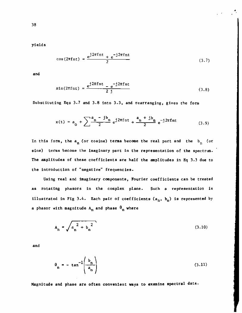
Using real and ~aginary components, Fourier coefficients can be treated
as rotating phasors in the complex plane. Such a representation is
illustrated in Fig 3.4. Each pair of coefficients (an' bn) is represented by
a phasor with magnitude ~ and phase en where
jr-----"
An = " an 2
+ b n 2
(3.10)
and
(3.11)
Magnitude and phase are often convenient ways to examine spectral data.

r1
t
Imaginary
I \ ~--- an --•• -11 .. ~ _______________ ~~~ ______ r-______ ~~~ .. Real
\ ~
Fig 3.4. Representation of Fourier coefficients by a rotating phasor in the complex plane.
39

40
Measurements in the Frequency Domain
Several types of measurements can be made directly with most of the
spectral analyzers that are currently available. The basic measurement is
the linear spectrum, generally of both an "input" signal and an "output"
signal. Other functions are defined using these two spectrums or their
complex conjugates.
Linear Spectrum. The linear spectrum, denoted by S (f), is x
simply the
Fourier transform of the signal. From Eq 3.8,
(3.12)
The linear spectrum provides both magnitude and absolute phase information
for all frequencies within the bandwidth for which the measurement was taken.
Since the absolute phase is measured, a trigger is required to synchronize
the signal for averaging. Linear spectrum averaging is useful for
determining predominant frequencies of excitation, identifying fundamental
modes and harmonics of a dynamic system, or extracting a "true" signal out of
background noise.
Auto Spectrum. The autospectral density function, G (f), commonly xx
called the autospectrum, is defined as the linear spectrum, S (f), multiplied x
by its own complex conjugate, S *(f). That is: x
G (f) '" S (f)· S *(f) (3.13) xx x x
The magnitude of the autospectrum is the magnitude squared of the linear
spectrum. This magnitude can be thought of as the power (or energy of a

41
transient, impulse signal) at each frequency in the measurement bandwidth.
However, multiplication by the complex conjugate eliminates the imaginary
components of the spectrum, so no phase information is provided by the
autospectrum. The advantage of the autospectrum is that it provides
information similar to that of the linear spectrum but does not require a
trigger to synchronize the averaging of signals. The autospectrum is the
Fourier transform of the autocorrelation function in the time domain.
Cross Spectrum. The cross-spectral density function, G (f), or cross yx
spectrum, is the Fourier transform of the cross-correlation function between
two different signals x(t) and yet). The cross spectrum is defined by
where Sy(f) is the linear spectrum of the output and Sx*(f) is the complex
conjugate of the linear spectrum of the input. The magnitude of Gyx(f) is a
measure of the mutual power between the two signals, making the cross
spectrum an excellent means of identifying predominant frequencies that are
present in both the input and output signals. The phase of Gyx(f) is the
relative phase between the signals at each frequency in the measurement
bandwidth. Since the phase is a relative phase, the cross spectrum
measurement can be made without a synchronizing trigger. The cross spectrum
is used primarily to determine the phase relationships between two signals
which may be caused by time delays, propagation delays, or varying wave paths
between receivers.

42
Transfer Function. The transfer function, H(f). or frequency response
function, characterizes the input-output relationship of a dynamic system.
The frequency response function is the ratio of the spectrum of the system's
response (output) to the spectrum of the system's excitation (input):
S (f) H ( f) = ~Y,,--:-:,.,....
S (f) x
(3.15)
Due to statistical variance of S (f) and S (£) for certain systems, a better y x
measure of H(f) can be obtained by using the autospectrum and cross-spectrum
functions. If both numerator and denominator are multiplied by S *(f), x
H(f) S (f) • S * (f) G (f) Y _x_,..--,- = -..y_x __
S (f) • S * (f) G (f) x x xx
(3.16)
Thus, the transfer function is similar to the cross spectrum. Both
provide the same information; the magnitude of the transfer function is
normalized by the autospectrum of the input Gxx(f) relative to the magnitude
of the cross spectrum. Consequently, the transfer function of a given system
should be constant regardless of the input (if the system does not undergo
nonlinear behavior). Generally, the input is a force measurement derived
from the signal of a load cell mounted on the source of excitation.
Depending on the quality which is measured as output, the transfer function
may provide a measurement of impedance, dynamic stiffness, or one of several
other system properties. The transfer function is frequently used to
identify natural frequencies and damping coefficients of a dynamic system.
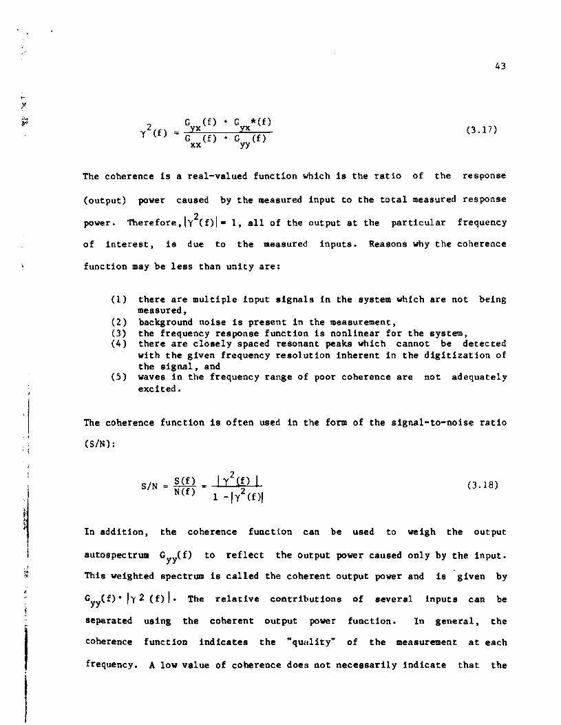
Coherence Function. The coherence function.ly2 (f)l, is a measurement
made in conjunction with the transfer function. Coherence is defined as,
j
. , , I
~ I
1
I
43
G (f). G *(f) yx yx
G (f) • Gyy
(f) xx
(3.17)
The coherence is a real-valued function which is the ratio of the response
(output) power caused by the measured input to the total measured response
power. Therefore,l y2(f)l- 1, all of the output at the particular frequency
of interest, is due to the measured inputs. Reasons why the coherence
function may be less than unity are:
(1) there are multiple input signals in the system which are not being measured,
(2) background noise is present in the measurement, (3) the frequency response function is nonlinear for the system, (4) there are closely spaced resonant peaks which cannot be detected
with the given frequency resolution inherent in the digitization of the signal, and
(5) waves in the frequency range of poor coherence are not adequately excited.
The coherence function is often used in the f~rm of the signal-to-noise ratio
(SiN) :
SIN = S(f) N (f)
(3.18)
In addition, the coherence function can be used to weigh the output
autospectrum Gyy(f) to reflect the output power caused only by the input.
This weighted spectrum is called the coherent output power and is given by
Gyy(f)· Iy 2 (f) I· The relative contributions of several inputs can be
separated using the coherent output power function. In general, the
coherence function indicates the "quality" of the measurement at each
frequency. A low value of coherence does not necessarily indicate that the

, I
44
measurement is invalid for a particular frequency but may suggest that more
averaging is required to improve the signal-to-noise ratio.
Additional Considerations for Digital Signal Analysis
Digital signal processes offer the advantages of quick and efficient
data measurement, analysis, and storage. The capability to average a series
of records enhances data measurement since noise and non-synchronized signals
will approach a mean value of zero. Digitization also permits convenient
manipulation of data for calculations and interpretation. However, the
conversion of an analog signal to a digital signal includes some drawbacks.
First, to ensure that the digitized signal accurately represents the
analog signal, the sampling rate of the "function" which converts the signal
must be at least twice the frequency of the highest frequency present in the
waveform being sampled. If the sampling rate is too low, higher frequencies
will "alias", or appear as lower frequencies in the spectrwn. This potential
problem is demonstrated graphically for the time record shown in Fig 3.5.
Generally, the instrwnentation is designed so that the selection of the
bandwidth for the measurement automatically adjusts the necessary filtering
and sampling rate.
Secondly, since computers or microprocessors can handle only a finite
amount of data, the signal must be truncated. Truncation is accomplished
with a function called a window. The simplest type of window is a
rectangular box. When the window "examines" an exact integral number of
cycles of all the frequency components, the resulting spectrum is accurate.
If a noninteger number of cycles occurs in the window, some of the magnitude
of a given frequency component may appear at adjacent frequencies. This

45
)Real" Signal "APparent"A
f\ I
.J
I I \ I
I J \ I
I \ \
I \ I \ I I \ I \ I
I I
\ \ I \ I
I \ I
I I
\ I
I \ \ I \ I
I \
,I
~ Discrete Sampling Points ("sampling Rate"1
I I I I I I I 1-
Pig 3.5. LoW-frequency alias resulting fro. insufficient sampling ofa high-frequency signal.
46
phenomenon is known as leakage. Invariably, some leakage is going to occur
for some frequencies in most signals. The type of signal (e.g., sinusoidal,
random, or transient) governs the type of window employed to minimize the
effects of leakage.
Lastly, the inherent inverse relationship between period, or length of
the time signal, and frequency creates problems with resolution, particularly
when the digital signal consists of a fixed number of data points. As the
time length of the signal increases, the bandwidth of the measurement in the
frequency domain narrows. Conversely, wider bandwidths require shorter time
records and provide less frequency resolution. Some instruments include
capabilities to overcome this dilemma. Rather than make a wide baseband
measurement from zero to some high frequency, the measurement is centered
about the high frequency with a narrow band. The band selectable analysis,
or .f zoom" measurement, allows high frequency resolution in a high frequency
range.
CHAPTER 4. SOIL TESTING AT WALNUT CREEK SITE
SITE DESCRIPTION
The Walnut Creek site is located about 5 miles (8 km) east of the campus
of The University of Texas at Austin, as shown in Fig 4.1. The land at the
site is part of the Walnut Creek Wastewater Treatment Plant, which is
operated by the City of Austin. The site is located about 600 ft (180 m)
from the public road in front of the treatment plant. As a result, traffic
movement or high tension wires do not contribute to the background noise
level. Power to operate electrical equipment is conveniently available from
a nearby storage building.
The topography at the site is relatively flat. The soil profile
consists of a deep clay deposit with a thin seam of gravelly material within
a few feet of the surface. The natural water content of the clay ranges from
16 percent at the surface to 30 percent at a depth of 30 ft (9 m).
Subsurface exploration by Patel (Ref 20) is recorded in the boring log shown
in Fig 4.2.
EXPERIMENTAL PROCEDURE
Two series of tests were performed on two different occasions at the
Walnut Creek site, hereafter they are referred to as WC-1 and WC-2. Test
47

48
" f
UNIVERSITY OF
~
I WALNUT
\./CREEK
\
Fig 4.1. Location of Walnut Creek test site.

{-o
SUBSURFACE EXPLORATION LOG Borehole: Bl
Depth (ft)
o
10
cu .... 0-e III
CIl
Soil Description
Dense fine to coarse gravel with cobbles
Dark clay with occasional gravel
Nov. 28, 1979
Atterberg Limits
LL % PL(%)
50 24
Fig 4.2. Soil profile at Walnut Creek site (Ref 20).
In Situ w(%)
16
20
22
20
49

P'
.'
50
Series WC-l was performed on October 23, 1980, while WC-2 was performed on
Karch 19, 1981. Both series of tests included similar spectral measurements.
The primary differences between the two series of tests were the types of
sources employed, the resonant frequency of the geophones, and the spatial
configuration of the geophones.
Test Series WC-1
The only source used in this first series of tests was a steel drop
hammer. (The steel drop hammer and subsequent sources are described in
detail in Section 4.3.) The drop hammer was used to impact the soil surface
directly and also to strike a steel plate resting on the soil surface. In
addition, the height of drop was set at both 6 in.
(61.0 cm) for the initial set of measurements.
(15.2 cm) and 24 in.
Two vertical geophone velocity transducers were used to capture the time
domain signal of the generated waves. Each geophone had an undamped natural
frequency of about 8 Hz and had a shunt resistance which provided a damping
of approximately 50 percent of critical damping. The frequency response
curves for the two geophones used for WC-1 were nearly identical up to
1600 Hz and were approximately linear over the range from 10 to 100 Hz, as
shown in Fig 4.3. The transduction constant was in the range of 1 volt per
in./sec (0.4 volt per cm/sec), although an exact calibration factor was not
obtained since only wave propagation velocities (and not absolute particle
velocities) were determined in this study.
The geophones were coupled to the soil surface by means of a 3-in.
(7.6-cm) long steel spike attached to the bottom of the geophone case. For
each measurement, the pair of geophones was located so that the distance
j

~ ".b .•• a ....... ·• 'W,"'~if.II._"I~J1~P;.1"·"~:·'!,~-.1,·'(",,·,'rt·.,.o·')Y: ....... ~ .,~~~:.....,.~1f''(. ...... , .. '' "" ·~~V"~-'!'r<f"V-
10.0-.---------------------------,
- -I I fit - 1.0-0 ->
CD lit c: 0 Q. lit CD 0:: CD c: 0
.r! 0.1-Q. 0 ID
(!)
U ,
0.01 , Frequency, Hz o 100
Fig 4.3. Response curves of the two vertical geophones used for test series WC-l.
VI t-"

52
between the geophones was the same as the distance from source to the first
geophone. For example, f~r the first set of measurements, the first geophone
was placed at a distance 4.0 ft (1.2 m) from the source and the second
geophone was placed at a distance 8.0 ft (2.4 m) from the source, so as to
maintain a spacing of 4.0 ft (1.2 m) between the two geophones. Since the
geophones could be conveniently placed at the desired location with the
attached spike, distances and spacings were controlled within a tolerance of
+ 0.02 ft (+ 0.6 cm). The geophones were aligned in a linear array extending
from the source location in a direction parallel with the centerline of the
cased boreholes at the site. Wave propagation was measured in the direction
from borehole B1 toward borehole B5. A complete diagram of the test set-up
is shown in Fig 4.4. Table 4.1 contains a summary of the measurements made
during Test Series We-1.
Test Series We-2
Three different sources were utilized in this second series of tests: a
sledge hammer striking an embedded concrete cylinder, the drop hammer
striking an embedded steel wedge, and a small hammer striking a rectangular
wooden plate resting on the surface. In each case, it was difficult to
control the exact nature of the hammer blow, although it was possible to
establish a "reproducible" hit for each source. Because of the size of the
embedded concrete cylinder, the embedded steel wedge and rectangular wooden
plate were located about one ft (0.3 m) closer to the geophones than the
concrete cylinder in order to maintain all sources and geophones in the same
linear array.

------..... --~-.,~. - ~~--~----.~~~~ .. ',. .ft .. '. Me ibt . " •• '1 ,$,
32 o
o BS
M
o B4
Direction of Wave Propagation •
~
o B3
4 o
2 o <3
/ Source Location
o B2
o Bl
~ 10 ft .1_ 10 U .1_ 10 ft _14 10 ft -I Lelend
o Existing boreholes used in work performed by Patel (1981).
~ .... ~--~ .. [J Location of geophones (with distance from source in feet).
Fig 4.4. Schematic layout of the l-lalnut Creek site for test series WC-I.
In W

•• ~."""".-,- ~ • .,~~ • !'In.).'.'. ~ .
TABLE 4.1. SUMMARY OF MFAStTREMENTS AT WALNUT CREEK FOR TEST SERIES WC-1
Record No. Distance from Distance Type of Source Height Number Bandwidth (Track No.) Source to between of of of
Geophones (ft) Geophonea Drop Averagea Spectrum
Nellr rar (ft) (in) (Hz)
35(1) 4.0 B.O 4.0 Hammer on Plate 6 5 200
40(1) 4.0 B.O 4.0 " " " 6 25 200
45(1) 4.0 B.O 4.0 " " " 24 25 200
50(1) 4.0 B.O 4.0 " .. " 24 25 1600
55(1 ) 4.0 B.O 4.0 .. .. " 24 5 1600
60(1) B.O 16.0 8.0 .. .. " 24 5 1600
5(2) B.O 16.0 8.0 .. " " 24 5 200
10(:1) B.O 16.0 B.O " .. " 24 '-5 200
15(2) B.O 16.0 B.O Ha_r on Soil 24 5 200
20(2) 16.0 32.0 16.0 " .. " 24 5 200
25(2) 2.0 4.0 2.0 " " .. 24 5 200
30(2) 2.0 4.0 2.0 " " .. 24 25 200
35(2) 2.0 4.0 2.0 " .. .. 24 5 1600
Computer Data File
Identi fication
SINCI
SHWC2, SHWC6
SINC3
SHWC4
----
SHWC7
SHWC5, SHWCI0
SHWCB
-SHWC9
I
\J1 J:-
• io--. . ,.L. ... . . , 77 q . -

·",
. "
55
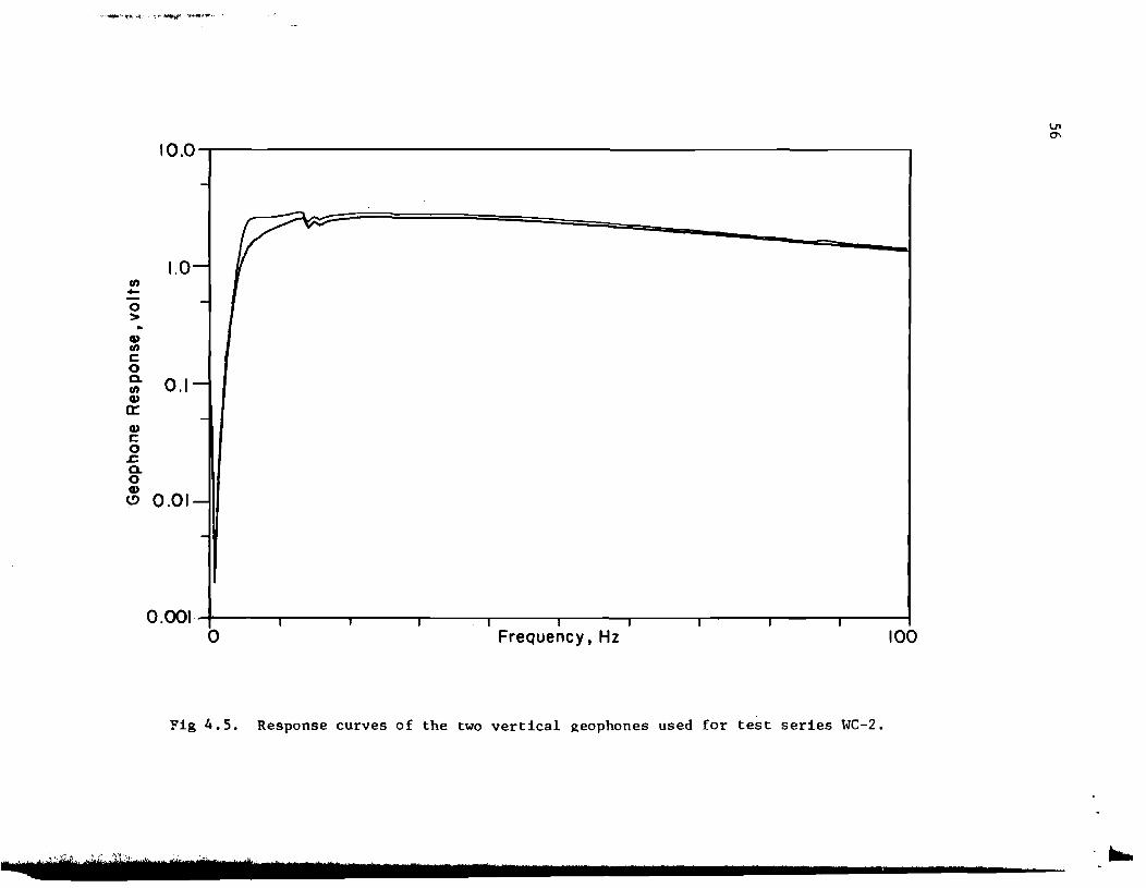
Vertical geophones used in Test Series WC-2 had an undamped natural
frequency of 4.5 Hz and a shunt resistance to provide approximately 50
percent of critical damping. The frequency response curves were nearly
identical up to 800 Hz and were approximately linear over the range from 5 to
100 HZ. as shown in Fig 4.5. Again. an exact calibration factor was not
determined since the calibration curves were nearly identical and particle
velocities were not determined.
For Test Series WC-2. the geophones were placed in augered holes to
minimize background noise and to provide better coupling between the
geophones and the soil. The holes were augered to a depth of 6 to 8 in.
(15.2 to 20.3 em). The geophones were then embedded at the bottom of the
hole by means of steel spikes and the remainder of the hole was backfilled
with the augered soil.
For each measurement. one geophone was always located at a fixed
distance of 2.25 ft (0.68 m) from the center of the concrete cylinder. This
geophone served as a "reference" geophone from which the second geophone was
located. The distance from the source (concrete cylinder) to the far
geophone ranged from 4 ft (1.2 m) to 32 ft (9.8 m). Since the holes were
augered by hand. the exact distances varied slightly from geophone to
geophone. The exact spacing between geophones for each set of measurements
is given in Table 4.2. The geophones were aligned in a linear array , f extending from the source in a direction parallel with the centerline of the
boreholes. Wave propagation was aeasured in the direction from borehole B4
to slightly beyond borehole Bl. A complete diagram of the test set-up is
+ shown in Fig 4.6. Table 4.2 contains a summary of the measurements made i
during Test Series WC-2.
.. ' .... ~.-'!"",,-l ~ ,,,~ :'1 ..... ,~~.
\J1 a-
10.0
LO-r
m -0 > CD m c: 0 0. 0.1-m CD 0: CD c: 0 E; 0. 0 CD
(,!) 0.01-
I I 0.001 , Frequency, Hz o 100
Fig 4.5. Response curves of the two vertical ~eophones used for test series WC-2.
'11, ~'.j, ,".r'~ '"f1 '.,~, . ....
.------' ......... ~, ...... ,. ... ~~"-"""-: ,;.,.,. ... ...., .. ',....... >- ,_ .. _ :4., ..... ". ___ ,~, _ ..... ______ . __ ~ :x .. · .&;" ··4 fa ".4 .. 1tS1·.,
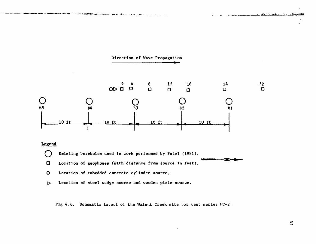
Direction of Wave Propagation
2 4 at> c c
8 o
12 o
16 o
24 o
00000 B5 B4 B3 B2 Bl
~ 10 ft .. I.. 10 ft ~14 10 ft ~. 10 ft ~ Lesend
<=) Existing boreholes used in work performed by Patel (1981). ----____ z _
o Location of geophones (with distance from source in feet).
() Location of embedded concrete cylinder source.
~ Location of steel wedge source and wooden plate source.
Fig 4.6. Schemat ie layout of the Walnut Creek site for test series T·TC-2.
32 o
VI ......

TABLE 4.2. SUMMARY OF MEASUREMENTS AT WALNUT CREEK FOR TEST SERIES WC-2
Record No. ApproxillUlte Exact Type of Source Number Bandwidth (Track No.) Dilt.nce frotl Diet.nce of of
Source to Far between Averagea SpectrulD Geophone Geophones (Hz)
(ft) Cft)
11(1) 4 2.08 Sledge Hammer on Conc. Cylinder 5 1600
16(1) 3 2.08 Drop Ha-.er on Steel Wedge 5 1600
21(1) 4 2.08 Sledge Ha ... r on Conc. Cylinder 5 400
26(1) 4 2.08 .. " .. .. .. 5 100
3U1) 3 2.08 Drop Ham.er on Steel Wedge 5 100
36(1) 3 1.08 911U111 Ha ... r on Wooden Plate 5 100
41(1) 8 6.04 Sledge Hammer on Conc. Cylinder 5 400
46(1) 8 6.04 .. .. II .. .. 5 100
51(1) 7 6.04 Drop Ha ... r on Steel Wedge 5 100
56(1 ) 12 9.94 Sledge Hammer on Conc. Cylinder 5 100
61(1) 16 14.10 II .. .. II II 5 100
62(1) 16 14.10 " .. " .. .. 5 25
680) 24 71.92 " .. " .. .. 5 100
69ft) 24 21.92 " .. .. " " 5 25
5(2) 32 30.00 " .. II II .. 5 100
COliputer Data File
Identification
SHWCll
SHWC14
SHWC12
SHWC13
SHWCI5
SHWC21.
SHWC22
SHWCl6
SHWC23
SHWC17
SHWC18
SHWC24
SHWC19
SHWC25
SHWC20
VI 00
~r51:11 7 I ...
',1,
~ 59
Recording of Spectral Measurements
Measurements were recorded and stored with a Hewlett-Packard 5423A
Structural Dynamics Analyzer. The dual-channel instrument includes a set of
signal filters, an analog-to-digital converter (ADC), a digital oscilloscope,
and a magnetic cassette tape for storage and recall of permanent records.
The analyzer can directly measure all of the time domain and frequency domain
measurements previously discussed in Chapter 3. In addition, the type of
signal, type and number of averages, bandwidth (or time length of the
record), and trigger conditions can all be specified by the operator. The
analyzer can be easily interfaced with an x-y plotter to provide a hard copy
of the data.
Each set of measurements was made with a pair of geophones since the
HP5423A analyzer is a dual-channel device. The measurement was triggered
internally by using the input signal from the first geophone in the pair.
The trigger level was adjusted to start the recording of the measurement in
the first half sine wave of the impulse as it passed by the first geophone.
A pre-trigger delay was used to capture the initial portion of the impulse
that would have otherwise been lost prior to triggering. Both channels were
programmed with the same pre-trigger delay so as not to introduce an internal
time or phase delay when calculating measurements using both signals. A more
detailed and complete explanation of the set-up procedure is contained in
Appendix A.
Frequency measurements (in contrast to time domain measurements) were
most often performed during both Test Series WC-l and WC-2. Stable (equal
weight) averaging was used for all measurements. The analyzer was programmed
to perform a frequency response function, commonly called the transfer

60
function. This measurement additionally provided the coherence function, the
cross spectrum, and che autospectrums for
measurements will be identified by the location of
both
the
signals.
pair of
Hereafter,
geophones.
For example, measurement V2-V24 identifies the measurement recorded with the
vertical geophone (V) nearer to the source located at 2 ft (0.6 m) and the
vertical geophone farther from the source located at 24 ft (7.3 m).
DESCRIPTION OF SOURCES
All of the sources used during both series of tests were available from
past or ongoing projects at The University of Texas at Austin. Due to time
and budget constraints, no new sources were developed in this particular
phase of the project.
Drop Hammer
The drop hammer consists of a 2.5-in. (6.4-cm) diameter cylindrical
steel mass with a length of 9 in. (23 em) and a weight of about 12 lb
(5.4 kg). The cylinder has a longitudinal center hole so that it can be
released to fall from any height along the 24-in. (6.4 em) long rod which
guides the hammer to impact on a steel base which is a180 2.5 in. (6.4 em)
in diameter. The amount of energy delivered by the impact is roughly
proportional to the height of drop.
The drop hammer is most easily used by s1aply resting the base directly
on the soil surface. To provide a larger striking surface, sa-e type of
plate can be placed between the soil and the base of the hammer. In Test
Series WC-l, a 0.75-in. (l.9-cm) thick steel plate with a 6-in. (l5.2-ca)
, r
61
diameter was used as a striking surface in conjunction with the drop hammer.
This arrangement is shown in Fig 4.7a.
Drop Hammer on Embedded Steel Wedge
An embedded steel wedge was selected as a typical source that could be
quickly and directly coupled with the soil. The wedge consisted of a 1/4-in.
(O.6-cm) thick, steel plate with a 2-in. (S.l-em) square shape. The plate
was welded to a short section of I-in. (2.S-cm) diameter pipe, which in turn
was welded to a steel head approximately 2.5 in. (6.4 em) in diameter. The
head can be struck by any hammer. The drop hammer was chosen for the
following reasons:
(1) the base of the hammer is the same size as the head of the wedge, (2) the drop hammer hit is vertical, and (3) the magnitude of the impact can be repeated fairly consistently.
The wedge can be embedded with little difficulty by a sledge hammer.
The wedge was driven such that the broad side of the plate was perpendicular
to the direction of wave propagation. This orientation provided a shearing
motion when the wedge was struck. As such, minimal P-wave energy was
generated. The drop hammer and steel wedge are shown in Fig 4.7b.
Sledge Hammer on Embedded Concrete Cylinder
An emhedded concrete cylinder already existed at the site from testing
performed by Patel (Ref 20). The top of the cylinder is located slightly
below the ground surface. The cylinder is approximately 16 in. (40 cm) in
diameter and 13 in. (33 em) deep. The location of the embedded cylinder at

j
62
(a) Drop Hammer on Steel Plate. (b) Drop Hammer on Embedded Wedg~.
(e) Sledge Hammer on Cone. Cylinder.(d) Small Rammer on Wooden Plate.
Fig 4.7. Illustration of sources used at Walnut Creek.

I
61
the site is shown in Fig 4.6. The cylinder was struck near its center by a
sledge hammer to generate wave energy. The source is shown in Fig 4.7c.
Small Hammer on Wooden Plate
This source was tested briefly to examine the effect of the material of
the striking plate on the magnitudes and frequencies of wave energy. The
plate was a 12 in. x 6 in. x 3/4 in. (30 em x 15 em x 2 em) plywood section
that rested directly on the ground surface. The plate was struck with a
small hammer with a nearly vertical hit. The plate and hammer are shown in
Fig 4.7d.
COMPARISON OF SIGNIFICANT PARAMETERS
Various parameters were investigated to determine their significance in
the measurement of Rayleigh wave velocities. The parameters that were
examined include
(1) number of averages to obtain a representative measurement, (2) range of frequencies to be included in the measurement bandwidth, (3) type or nature of source, and (4) spatial distribution of geophones from the source point.
Number of Averages
Measurements were made during Test Series WC-1 to determine the effects
of varying the number of averages to obtain a "representative" spectral
measurement. The HP5423A Analyzer was set up to accept or reject a
particular transient event. Events were accepted only when they were judged

64
to be representative of the reproducible impact of the source. A specified
number of these events were included in a stable (equal weight) average.
Naturally, as the number of events of "averages" increases, the more
representative the overall average or total measurement will be. However,
for a method to be a quick and efficient testing technique, a small number of
averages is desirable. Ideally, one representative event would be adequate.
As a safeguard against capturing an event which for some reason is not
representative, several averages should be taken.
Since it is not clear how many averages are necessary or when averaging
has become excessive and unnecessary, sets of measurements from Test Series
WC-I were compared. Comparisons were made with measurements consisting of
five averages and with measurements consisting of 25 averages. The
measurements were compared directly by examining the similarities of the
phases of the cross spectrum.
by examining the coherence
measurement.
In addition, comparisons were made indirectly
function for the relative quality of each
Results of these comparisons for measurement(s) V8-V16 are shown in
Fig 4.8. The dashed lines represent the measurement made with five averages;
the solid lines represent the measurement made with 25 averages. The plot in
Fig 4.8a indicates that the phase information provided by the 5-average
measurement nearly matches that provided
There are no significant differences
by the
between
25-average measurement.
the coherence functions
associated with the two measurements, as shown in Fig 4.8b, suggesting that
the additional averages do not contribute to a better-quality or more-valid
measurement.
Similar results were obtained for other sets of measurements. The
5-average measurements provided essentially the same phase information and
J

t 180
m 1 ~ ~ ~ ~ ~ ~
~ m ~
f
-180-r--~~--~--~----~--~-J~----~--~----~--~
o Frequency, Hz 200
(a) Phase of the cross spectrum.
1.0-r--~~--~----~~----~----~----------------~
o Frequency, Hz
(b) Coherence function.
Fig 4.8. Comparisons of the use of the average of 5 observations with the average of 25 observations to obtain representative spectral measurements.
200
65

66
coherence values as the 25-average measurements regardless of the spatial
distribution of the geophones, the frequency bandwidth of the measurement, or
the amount of energy delivered by the drop hammer (varied by the height of
drop). These results led to the conclusion that five averages provided a
measurement that was as "accurate" as could be expected for any reasonable
number of averages. Subsequently, measurements taken during Test Series WC-2
were compiled with only five averages.
Measurement Bandwidth
The frequency bandwidth of a measurement is a significant parameter for
two reasons. First, the range of frequencies (or wavelengths) must be
adequate to sample appropriate depths of the soil profile. Second, the
resolution or "accuracy" of the measurement is controlled by the number of
points used to convert the analog signal to a digital signal. The HP5423A
Analyzer uses a fixed number of points (1024) for all measurements,
regardless of bandwidth, which means that as the range of frequencies is
extended, the resolution becomes poorer (6f between points becomes larger).
Inasmuch as wide bandwidths and fine resolution are in opposition with each
other, SOMe trade-offs must be made.
Comparison measurements for Test Series WC-l included bandwidths of 200
and 1600 Hz, while comparison measurements for Test Series WC-2 included
bandwidths of 25, 100, 400, and 1600 Hz. With few exceptions, no significant
differences were found between values of phase of the cross spectru.
function, regardless of the resolution associated with the bandwidth.
Figure 4.9a shows a comparison phase plot for bandwidths of 200 and 1600 Hz
for measurements VS-V16 from Test Series WC-l, while Fig 4.9b shows a similar
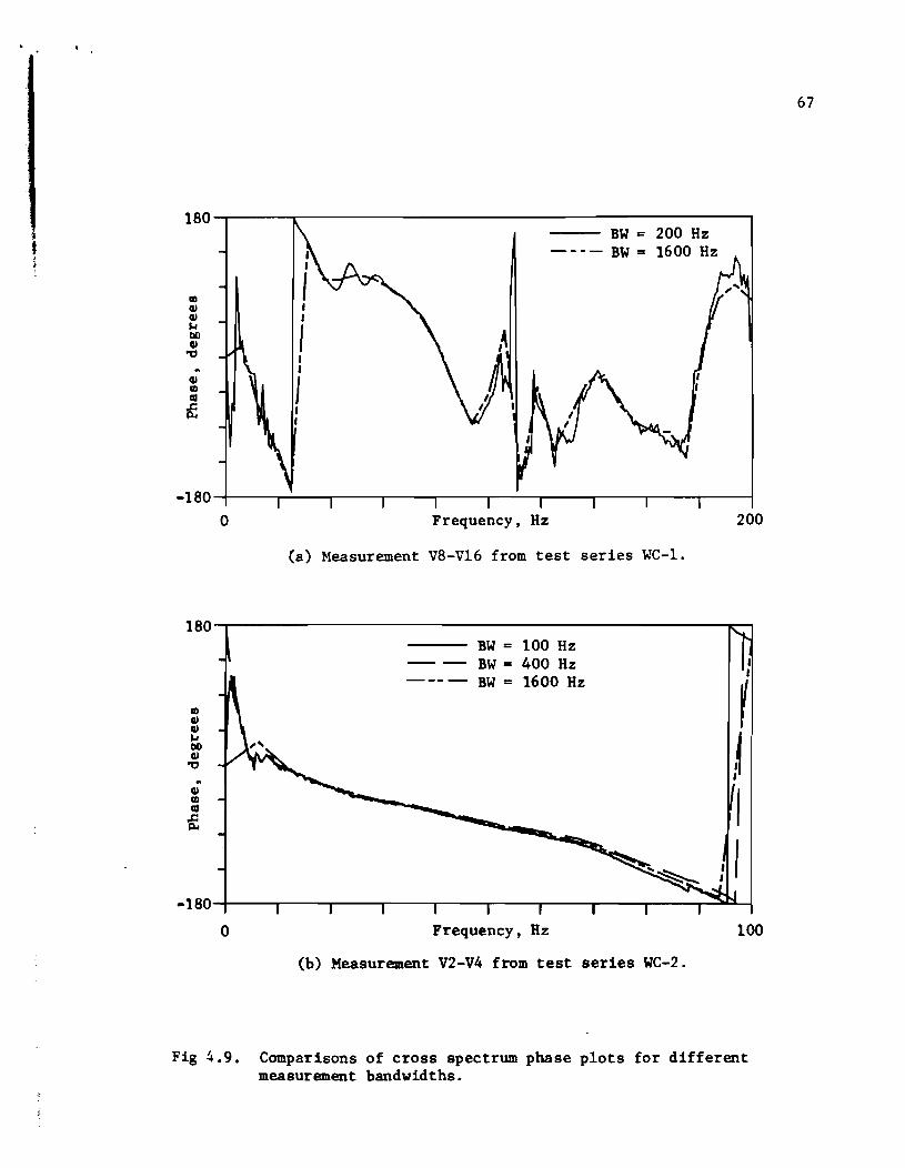
180-r----~----------------------------------------~
III CII CII ~ bO CII ." ~
CII III III
if
I I
I I I
J
BW = 200 Hz ---- BW = 1600
-180-r----r---_r----~--~--~~--~--~----~--~--~
o Frequency, Hz 200
(a) Measurement V8-V16 from test series WC-l.
180-r----------------------------------------------~
III CII CII ~ bO CII ." ~
CII III III
f
BW = 100 Hz 400 Hz 1600 Hz
-180-r--~r_--,_--~----r_--_r--_,~--~--~----~~~
o Frequency, Hz 100
(b) Measurement V2-V4 from test series WC-2.
Fig 4.9. Comparisons of cross spectrum phase plots for different measurement bandwidths.
67

68
comparison for measurements V2-v4 from Test Series WC-2. The frequency-phase
data from Fig 4.9b are reduced and plotted as a velocity-wavelength chart in
Fig 4.10. The slight variations in phase translate into a difference in
velocities of at most 8 percent. This difference is within the range of
experimental scatter associated with velocity measurements.
Although the range of the bandwidth (and inherently the degree of
resolution) is generally not a critical parameter in the cross spectrum
measurement, there are a few cases where special consideration is required.
First, if the measurement bandwidth is too large, the resolution may not be
fine enough to measure sharp changes in frequency response that occur over a
range of frequencies smaller than 6 f, the degree of resolution. Such an
occurrence is illustrated in Fig 4.9a, where the measurement with bandwidth
(BW) equal to 1600 Hz exhibits much less sensitivity to slight variations in
phase than the measurement with BW equal to 200 Hz which has a much finer
resolution. Since frequency and wavelength are inversely related, increasing
wavelengths correspond to decreasing frequencies. Resolution is most
critical at these lower frequencies where 6f may approach the same order of
magnitude as the frequencies being measured. This problem is illustrated in
Fig 4.11. Measurements with 25-Hz and 100-Hz bandwidths are compared. As
the wavelengths increase, the resolution becomes more critical, and the
scatter. in velocities (between measurements) increases.
A second consideration involves high frequencies or short wavelengths-
In a material with significant damping, such as soil, high frequencies will
attenuate very rapidly. Meaningful information may not be provided at high
frequencies, depending on several factors, including the type of source and
the spatial distribution of the geophones (to be discussed in subsequent
sections). Poor coherence at high frequencies (above about 250 Hz in
J,
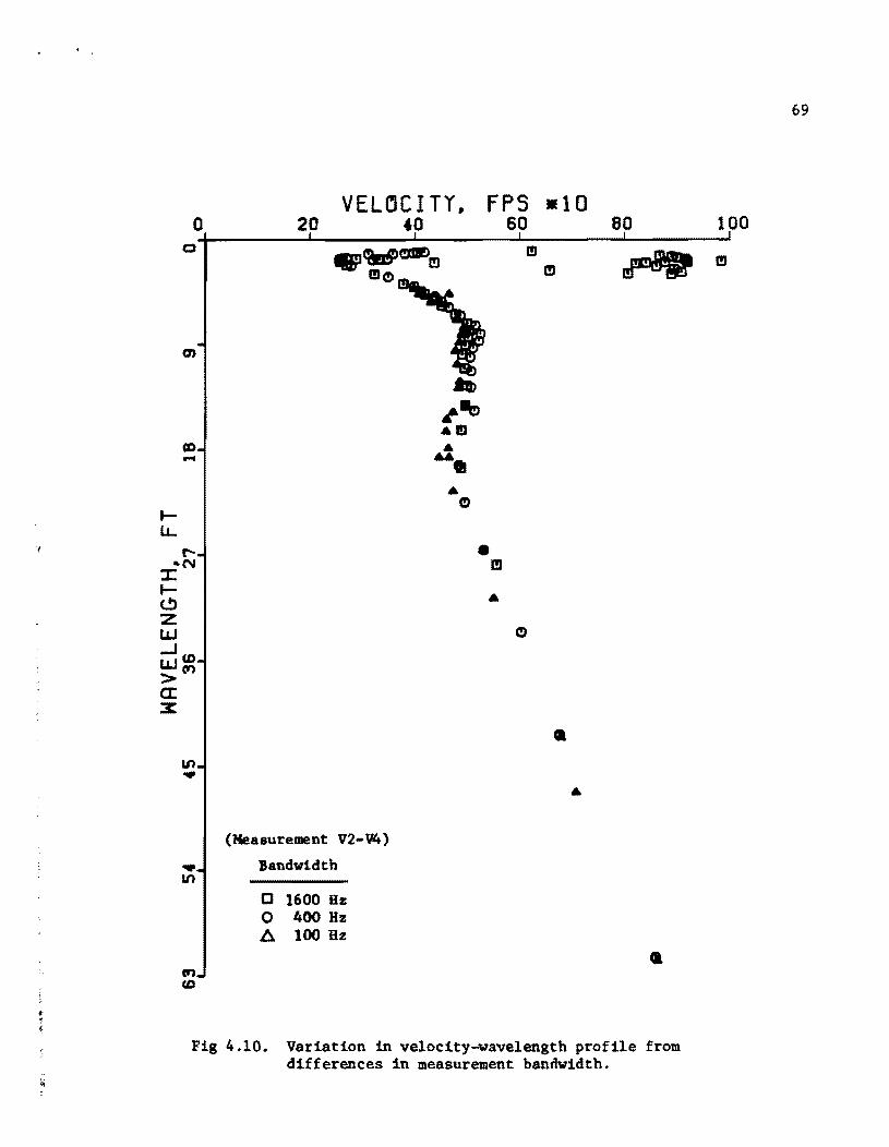
VELOC I ry, o 20 40
o
(Measurement V2-V4)
• Bandwidth U1
o 1600 Hz o 400 Hz 6 100 Hz
FPS -10 60
m m
80 100
.. Fig 4.10. Variation in velocity-wavelength profile from
differences in measurement bandwidth.
69
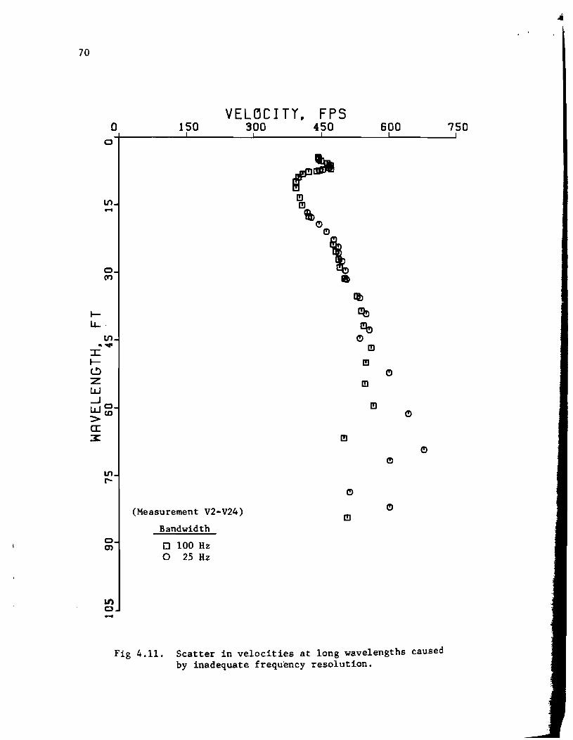
70
VEL~C I TY, FPS 0 150 300 450 600
e
1Il ....
e (Y')
I-I.L .
1Il •• :J: l-t!) Z W ....J we >(0 cr: 3:
1Il r--
e en
an o ....
r:' I!] I!]
'&>(!)
(!)
\ • 'I> l!b I!b
(!) I!]
I!] (!)
I!]
I!] (!)
I!]
(!)
(!)
(Measurement V2-V24) (!)
I!]
Bandwidth
0 100 Hz 0 25 Hz
Fig 4.11. Scatter in velocities at long wavelengths caused by inadequate frequency resolution.
750
71
Fig 4.12a) indicates that significant attenuation of the short wavelengths
has occurred and is generally accompanied by erratic phase information, as
shown in Fig 4.l2b.
Selection of an appropriate measurement bandwidth primarily depends on
which frequencies are required to "sample" desired depths. Naturally, these
frequencies may vary slightly from site to site depending on the soil
properties, particularly the wave velocities. For a given site, it is
relatively easy to develop a frequency-wa'ielength profile from the reduced
data which will indicate the appropriate frequency bandwidth necessary to
investigate the site. Such a plot for the Walnut Creek site is shown in
Fig 4.13. The plot indicates that wavelengths as short as 4 ft (1.2 m) can
be observed by using a measurement bandwidth of 100 Hz. If data closer to
the surface is required, a larger measurement bandwidth must be used to
observe the shorter wavelengths.
Typically, a bandwidth of 100 Hz will provide both an adequate range and
an adequate resolution (6f ~ 0.8 Hz with the HP5423A) for a reasonable depth
below the surface. For velocities at depths below about 25 ft (7.6 m), it
may be advantageous to lower the bandwidth (say to 25 Hz) and increase the
resolution. Conversely, if velocities within a foot or two of the surface
are desired, it will be necessary to increase the bandwidth severalfold.
Because sampling depth, or wavelength, is also related to the spacing between
geophones, the appropriate bandwidth should be selected in conjunction with
this spacing.

72
I ~
I u ~ ~ ~ ~
I ~ 0 u
I I
0.0
0 Frequency. Hz 400
(a) Coherence function.
180-r--~---'----~----------'---------------~
o Frequency, Hz 400
(b) Phase of the cross spectrum.
Fig 4.12. Effect of attenuation of high frequencies (short wavelengths) on spectral measurements.

I--1.L.
o o
N -
• N
o co
+
+ + i+
++ +
N + f'
• CD
20 FREQUENCY, HZ
40 60 80 100
Test Series WC-2 (Measurements V2-V4 through V2-V32)
Fig 4.13. Frequency versus wavelength plot a Walnut Creek site.
73

74
Sources
There are several characteristics which are important in the evaluation
of a feasible source. Among these are the magnitude of the impact, or how
much energy is delivered to the soil; the coupling of the source t~ the soil,
or how well the source transfers energy into the soil over the range of
frequencies required to sample the site adequately; and, last, the type(s) of
wave energy which are being generated or are at least the predominant energy
type(s). All of the sources used at Walnut Creek involved a hammer blow
which generated a transient impulse in the soil.
Test Series WC-1. Two sets of measurements were conducted to compare
the effect of the magnitude of the impact on the cross spectrum measurement.
With all other parameters held constant, one set of measurements was made
with the drop hammer released at a height of 6 in. (15.2 em) above the base
(resting on the steel plate), while another set was made with the drop hammer
released at a height of 24 in. (61 em). The similarities of the coherence
functions of these measurements are shown 1n Fig 4.14a and suggest that the
variation in drop height did not affect the range of frequencies excited by
the hammer-plate source. The relative magnitudes of the cross spectrums
(expressed in voltage squared) are shown in Fig 4.14b. Both spectrums
exhibit similar excitation up to about 120 Hz. The values of phase for the
two measurements agree very closely, except in the range of about 40 to 80 Bz
where the coherence for both measureaents is relatively low. This suggelts
that the magnitude of the impact is not a critical factor as long al
sufficient energy is input to " sample" the desired depth of a site.
Comparison measurements were also made using the drop hammer resting on
the steel plate and the drop hammer resting directly on the soil at the
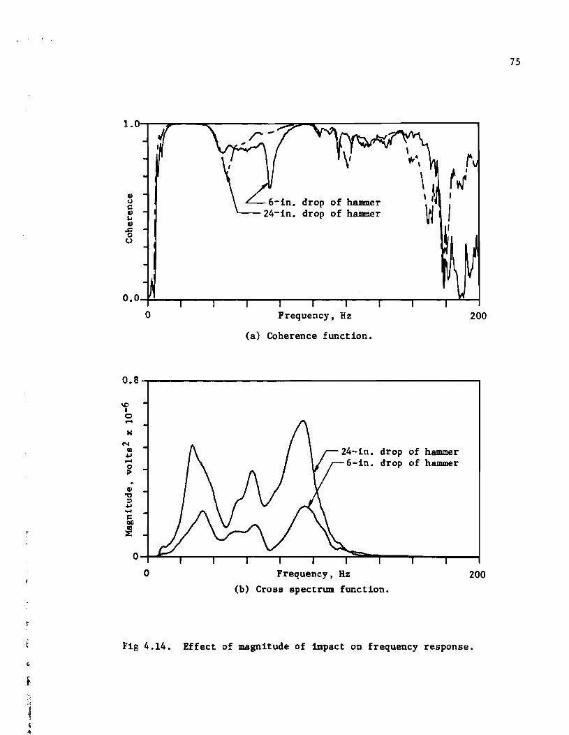
rl
;
1,~--~----~--------~~~--~------------------,
drop of hammer drop of hammer
\
"'\ r \ ~ tJ 'I I
VJ I
~
O.O,-+----~--_T----~--~----~--~----,_--~----,_~~
0.8
\D I 0 ~
~
N II)
~ ~
0 ;>
QI
"tI :I ~ ~
c 00
~
0
o
0
Frequency, Hz
(a) Coherence function.
Frequency, Hz
drop of hammer drop of hammer
(b) Cross spectrum function.
200
200
Fig 4.14. Effect of magnitude of tmpact on frequency response.
75
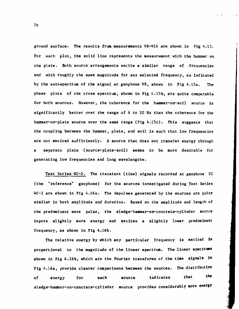
76
ground surface. The results from measurements V8-V16 are shown in Fig 4.15.
For each plot, the solid line represents the measurement with the hammer on
the plate. Both source arrangements excite a similar range of frequencies
and with roughly the same magnitude for any selected frequency, as indicated
by the autospectrum of the signal at geophone va, shown in Fig 4.15a. The
phase plots of the cross spectrum, shown in Fig 4.15b, are quite comparable
for both sources. However, the coherence for the hammer-on-soil source is
significantly better over the range of 6 to 20 Hz than the coherence for the
hammer-on-plate source over the same range (Fig 4.15c). This suggests that
the coupling between the hammer, plate, and soil is such that low frequencies
are not excited sufficiently. A source that does not transfer energy through
a separate plate (source-plate-soil) seems to be more desirable for
generating low frequencies and long wavelengths.
Test Series WC-2. The transient (time) signals recorded at geophone V2
(the "reference" geophone) for the sources investigated during Test Series
WC-2 are shown in Fig 4.16a. The impulses generated by the sources are quite
similar in both amplitude and duration. Based on the amplitude and length of
the predominant wave pulse, the sledge-hammer-oD-concrete-cylinder source
inputs slightly more energy and excites a slightly lower predominant
frequency, as shown in Fig 4.16b.
The relative energy by which any particular frequency is excited 1.
proportional to the magnitude of the linear apectrum. The linear spectr~.
shown in Fig 4.16b, which are the Fourier transforms of the time signals io
Fig 4.16a, provide clearer comparisons between the sources. The distribution
of energy for each aource indicates that the
sledge-hammer-on-concrete-cylinder aource provides considerablY more eoerlJ
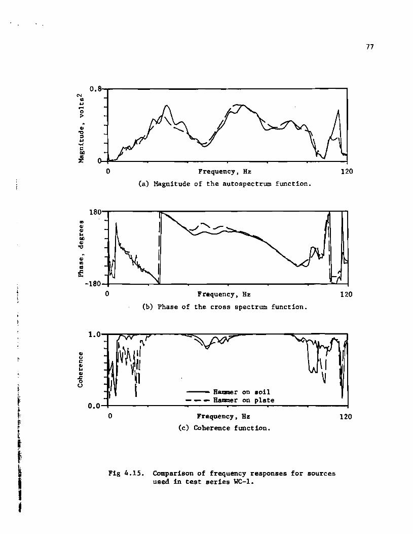
N III ~ .... o :>
III QI QI ~ lID QI
'C .. QI III CIS
f
QI U C 4i ~ QI
.s:: 0 u
o.~~----------------------------------------------~
180
-180
1.0
0.0
o Frequency, Hz
(a) Magnitude of the autospectrum function.
0 Frequency, Hz
(b) Phase of the cross spectrum function.
~ '\
~~J,~ ~I Haaaer on 80il
--- Hammer on plate
0 Frequency, Hz
(c) Coherence funct ion.
Fig 4.15. Comparison of frequency responses for sources used in test series We-I.
120
120
120
77
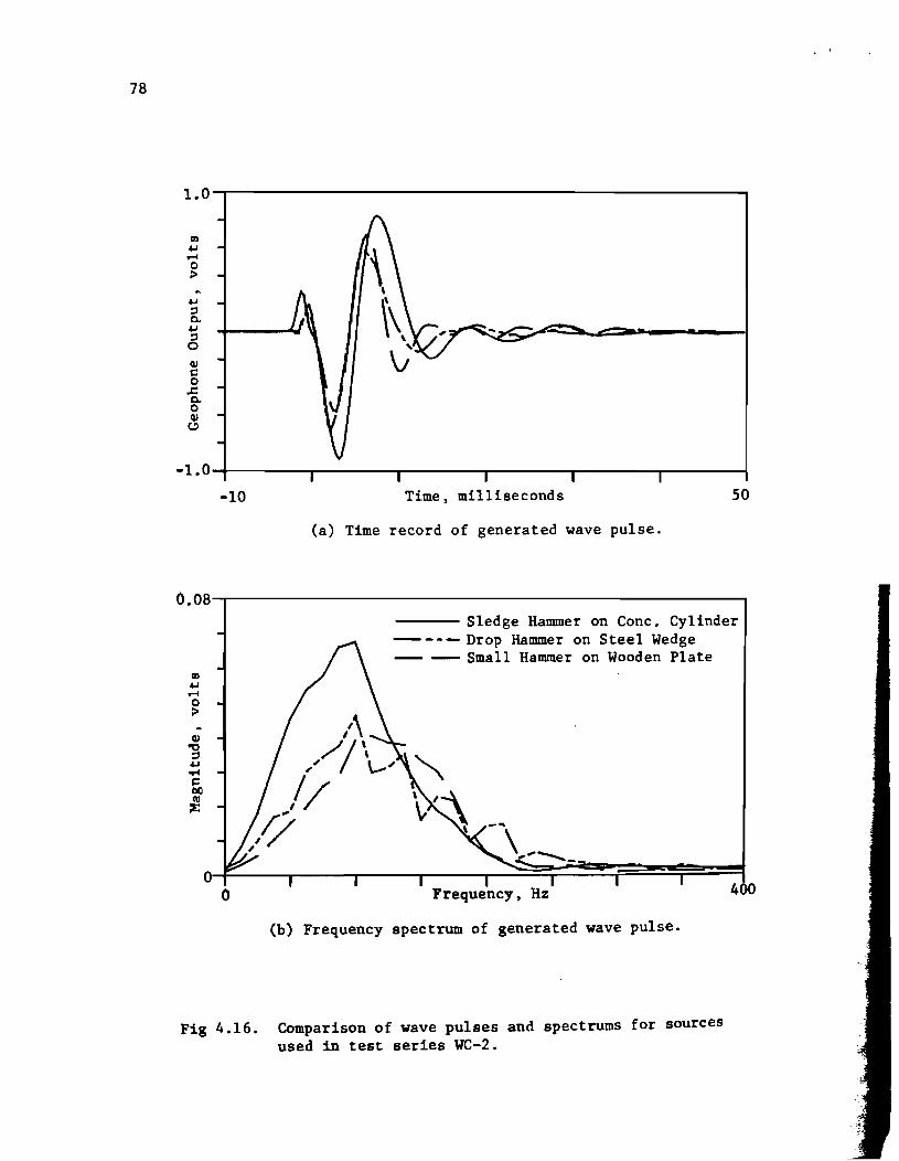
78
1.0-r--------------------------------------------~
4-1 :l c..
4-1 :l o CII t: o .c c.. o CII t!)
-1.0-r------,-------.-------.-------r-----~------~
-10 Time, milliseconds 50
(a) Time record of generated wave pulse.
O.08-r------------------------------------------~
------- Sledge Hammer on Conc. Cylinder
CD 4-1 ...-I o :>
o
------ Drop Hammer on Steel Wedge --- --- Small Hammer on Wooden Plate
Frequency, Hz
(b) Frequency spectrum of generated wave pulse.
Fig 4.16. Comparison of wave pulses and spectrums for sources used in test series WC-2.
400

79
at frequencies below about 100 Hz, which is the range of frequencies needed
to investigate the Walnut Creek site (Fig 4.13). Over this range, the
drop-hammer-on-stee1-wedge source generates about 50 to 75 percent of the
energy that the sledge-hammer-on-concrete-cylinder generates, while the
sma11-hammer-on-wood-p1ate generates only 25 to 50 percent of the energy that
the sledge-hammer-on-concrete-cy1inder generates.
However, if the frequency response based on the transfer function is
examined, a different conclusion is reached about the effectiveness of wave
propagation by each source. Transfer functions based on measurements V2-V4
are shown in Fig 4.17. The magnitude of the transfer function is a
dimensionless ratio of the energy of the output signal (V4) to the energy of
the input signal (V2). Since the measurement is in effect "normalized" by
dividing the output by the input, the amount of input energy is not critical
for comparison purposes, as was the case for the linear spectrums compared in
Fig 4.16b.
Any apparent differences in attenuation of wave energy (indicated by an
output/input ratio less than one) must be a result of the geometric damping
of the various components of wave energy in the impulse produced by the
source, because the distance between the two geophones is the same and the
same material properties are being measured. At the surface of an elastic
half-space, body waves (P- and S-waves) follow a geometrical damping law of
2 l/r and R-waves follow a geometrical damping law of l/~ Therefore, body
waves attenuate more rapidly than Rayleigh waves. For the transfer functions
shown in Fig 4.17, a lower output/input ratio indicates more geometrical
damping, which can be interpreted as a greater percentage of body wave energy
in the impulse produced by the particular source.

1.0 II
41 'g 4.1 .... s:: till
~ s:: o .... 4.1 U s:: :J
fa< 104 41
'1-1 at C CIt 104 f-4
Sources
Sledge Hammer on Concrete Cylinder Small Hammer on Wooden Plate Drop Hammer on Steel Wedge
0.0-+-1 --..-----.---r-----.---_---r---..---__ --~-__t o Frequency, Hz 100
Fig 4.17. Comparison of transfer functions for sources used in test series WC-2.
00 o

J
I t i
81
The sledge-hammer-on-concrete-cy1inder source exhibits the highest
output/input ratio. The output/input ratio of the sma11-hammer-on-wood-p1ate
source is about 80 to 90 percent of the ratio of the
sledge-hammer-on-concrete-cy1inder source, while the output/input ratio from
the drop-hammer-on-stee1-wedge is about 50 to 55 percent of the ratio of the
sledge-hammer-on-concrete-cy1inder. These results indicate that the
drop-hammer-on-steel-wedge source contains more body wave components and is
less desirable as a Rayleigh wave source. This is not unexpected, since the
wedge was oriented so as to produce a shearing motion.
Based on the comparison of the sources in terms of their linear
spectrums (Fig 4.16b) and their energy transfer characteristics (Fig 4.17),
it can be concluded that the magnitude of energy generated by a particular
source is not the most critical characteristic of the source. More important
is the coupling, or energy transfer, of the source to the soil. With respect
to this criterion, a large flat mass in contact with the soil (preferably
without an intermediate plate) is the most desirable type of source.
Further evidence that the type of wave energy generated is an important
factor is shown in Figs 4.18 and 4.19. The phase of the cross spectrum for
each source (measurement V2-V4) shown in Fig 4.18a indicates that there is a
fair amount of scatter in phase between the sources, particularly at larger
frequencies. This translates into substantial scatter in the
velocity-wavelength profile, as shown in Fig 4.19. One possible explanation
of these differences in velocity may be varying percentages of body wave
energy in the signal, which affects the overall velocity of the impulse.
The coherence functions, shown in Fig 4.18b, indicate that the
sledge-hammer-on-concrete-cy1inder source excites low-frequency (about 6 to
82
180-.------------------__________________________ ____ ..
Q) IQ
a:I
'If
o
Sledge Hammer on Cone. Cylinder --- - - - Drop Hammer on Stee 1 Wedge --- ---- Small Hammer on Wooden Plate
Frequency, Hz 100
(a) Phase of the cross spectrum.
1.1-.--------------------------------------------------------~
Q) u c Q) k Q)
1i u
O.O~---_.------._---~--_r--_.---~~---T_--~--~--~
o Frequency, Hz 100
(b) Coherence function.
Fig 4.18. Comparison of cross spectrums and coherence functions for sources used in test series HC-2.
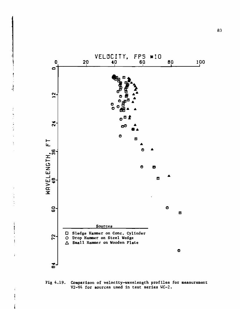
o U)
• CD
Sources
D Sledge Hammer on Cone. Cylinder o Drop Hammer on Steel Wedge ll. Small Hammer on Wooden Plate
Fig 4.19. Comparison of velocity-wavelength profiles for measurement V2-V4 for sources used in test series WC-2.
83
84
20 Hz) wave energy markedly better than the other sources. Again, this is
probably due to the excellent coupling of the mass with the soil.
Spatial Distribution of Geophones
The appropriate spacing of the geophones depends on the velocities of
the materials found at the site and the depth to which the investigation will
be conducted. The wavelengths, frequency bandwidth, and attenuation
properties of the site are all interrelated and affect the necessary spacing
of the geophones. Determination of upper and lower bounds for the spacing
(~x) between geophones as a function of wavelength is discussed in the
following paragraphs.
Consideration is first given to an upper bound for ~ x. This bound is
related to the attenuation of
examining the range of frequencies
the wave energy and can be established by
2 over which the coherence value (y)
remains near unity. Such a range indicates which frequencies have sufficient
energy at the output geophone (far geophone) to be accurately measured as a
response similar to that at the input geophone (near geophone). Since wave
attenuation is a function of distance, variations in ~x will give different
ranges of frequencies over which useful information is recorded.
The level of coherence that defines "useful information" is somewhat
arbitrary. For the purposes of developing a relationship between~x and f, a
coherence of y2 > 0.90 has been selected as indicative of useful information.
Relationships of frequency range (upper limit) to spacing are shown 1n
Table 4.3 for Test Series WC-l and 1n Table 4.4 for Test Series WC-2. Both
sets of data indicate a marked decrease in the range of useful frequencies as
the spacing increases. In other words, closer spacing is required to sample

TABLE 4.3. USEFUL FREQUENCY RANGE AS A FUNCTION OF RECEIVER SPACING FOR TEST SERIES WC-I.
Distance from Source to Geophone Range of Frequencies
Geophones (ft) Spacing, with Coherence> 0.9 -Near Far 6.x (ft) (Hz)
2 4 2 800*
4 8 4 326
8 16 8 207
16 32 16 84
*Based on useful information in phase plot of cross spectrum.
TABLE 4.4. USEFUL FREQUENCY RANGE AS A FUNCTION OF RECEIVER SPACING FOR TEST SERIES WC-2.
Distance from Source Geophone Range of Frequencies
Geophones (ft) Spac ing, with Coherence> 0.9
Near Far 6.x (ft) (Hz)
2 4 2 625
2 8 6 240
2 12 10 91
2 16 14 87
2 24 22 73
2 32 30 58
85

R6
higher frequencies. This is particularly true for soils, which rapidly
attenuate high-frequency-wave energy.
The data in Tables 4.3 and 4.4 are plotted in Fig 4.20. It appears that
the relationship between 6 x and f does not depend on the location of the
geophone nearer the source but only on the spacing between the geophones.
The data can be reasonably approximated by a straight line on a logarithmic
plot and can be described by an equation of the form
f '" k (luc) (4.1)
where k is a constant (the intercept at x -1) and m is the slope of the
line. The value of k is approximately 1360 and the slope of the line is
m = tan (-44°) = - 0.966 ~ - 1.0
Since the values of f plotted in Fig 4.20 represent an upper limit, the range
of frequencies over which useful information is provided (as a function of
spacing) is
f < 1360 - 6x
(4.2)
The constant 1360 has units of fps where f is in cps and 6x is in ft.
This constant represents 80il conditions at the Walnut Creek site and will
most likely vary depending on the particular site profile. Note that Eq 4.2
can serve as a guide for selecting an appropriate bandwidth for a given
spacing.

, ;
1OO0~1mm
100
N = .. >-CJ s:: ~ V I» ... rz.
10
1 10 100
Geophone Spacing (AX). feet
Fig 4.20. Relationship between geophone spacing and frequency range of useful information.
87
88
If the quantity V!LR
replaces f in Eq 4.2, a relationship between
wavelength and spacing is obtained as follows:
(4.3)
where velocity, VR, is in fps and wavelength, LR, is in ft. For a range of
S-wave (or R-wave) velocities of about 450 fps to 700 fps, which is typical
of soils, Eq 4.3 yields a range of LR greater than or equal to about
one-third 6x to one-half ~x. Conversely, to insure that the wave energy of a
particular wavelength does not decay excessively, the spacing between
geophones should not exceed two to three times the wavelength to be sampled.
This outcome verifies that excessive cycles of a particular wavelength or
frequency will lead to undesirable attenuation as far as signal pickup is
concerned.
The establishment of an upper bound for spacing between geophones should
be guided by the wavelength(s) to be measured. Based on the foregoing
discussion, it is preferable that 6 x not exceed two times the wavelength to
be measured. It is also reasonable to assume that the spacing between the
source and the first geophone should follow a similar criterion.
Consideration is now given to the lower bound for ~x. This bound is
influenced by the sensitivity of the instrumentation to measure phase
differences between signals. If the wave had travelled one wavelength by the
time it reached the first geophone, then, in theory, the second geophone
could be located as close as possible to the first geophone to measure the
relative phase differences. However, the precision of the instrumentation
and the desired accuracy in the phase difference create a physical limitation
that governs the proximity of the geophones to each other. The performance

89
specifications of the HP5423A Analyzer list the channel-to-channel phase
match as + 5 degrees. Thus, a cross spectrum phase measurement of 50 degrees
may potentially (though most likely will not) be in error by 10 percent. If
the spacing 6 x is at least one-third of the wavelength, then the phase
measurement will always be at least 120 degrees, and the percent error will
be less than about 4 percent. Note that this does not mean that all
measurements are in error by 4 percent, but that certainly no measurement is
in error by more than 4 percent.
For a given spacing, then, the longest wavelength which can be reliably
measured (with certainty of no more than 4 percent error) is three times 6x.
Longer wavelengths will not have travelled a distance sufficient to change
the phase by at least 120 degrees leading to potential errors greater than 4
percent. This establishes the lower bound for spacing between geophones to
be such that 6x is greater than or equal to L R/3. It should be recognized
that this is a very conservative lower bound, since it eliminates from
(confident) consideration any phase measurements less than 120 degrees. In
general, observed phase measurements even as low as 20 degrees for short
spacings (6 x ~ 2 - 6 ft) have provided reasonably representative wave
velocities. This is probably a benefit of using several averages to make the
measurement.
In summation, spacing is directly related to the wavelength(s) to be
measured. Based on the preceding discussion, a particular wavelength LR is
most accurately (or confidently) measured within a range of spacings given by
(4.4)
For application in field testing, it is more convenient to establish a
particular spacing and then to consider the range of wavelengths over which a
90
reliable measurement was made for that spacing. This relationship is
obtained by rearranging Eq 4.4 to yield
(4.5)
For example, if the spacing in the field was selected as 10 ft (3 m), the
range of wavelengths which could be measured with reasonable confidence and
accuracy would be about 5 to 30 ft (1.5 to 9 m). In general, if Ax is
increased geometrically--by doubling or
geophones--for each successive measurement,
tripling
then all
the spacing between
wavelengths will be
sampled properly during at least one measurement. More than likely, some
overlap of wavelength measurements will occur, to provide continuity in the
dispersion (velocity versus wavelength) curve.
The range given by Eq 4.5 can be employed to filter out those
wavelengths (or frequencies) which are not appropriate for a designated
spacings. By filtering out long wavelengths from close spacings and short
wavelengths from far spacings, much of the scatter associated with a set of
measurements is eliminated. Then only those wavelengths which fall within
the appropriate range are used to develop the velocity-wavelength profile.
The benefits of such an approach are illustrated in Figs 4.21-4.24. The
velocity-wavelength profile for Test Series WC-2, without filtering the
inappropriate wavelengths according to Eq 4.5, is shown in Fig 4.21. As a
result, there is excessive scatter for very short waves (less than 10 ft) as
well as for relatively long waves (greater than 50 ft). When the
inappropriate wavelengths are filtered, much of the scatter is removed, a.
indicated 1n Fig 4.22. Similar results are shown for Test Series WC-I. The
velocity profile in Fig 4.23 contains unfiltered wavelengths, while the
improved profile using filtered wavelengths is shown in Fig 4.24.

lLl..
a o
II) .....
o 0')
II) o .....
VELCJC I TI. FPS -10 20 40
Geophone Spacing
o V2-V4 o V2-VS ~ V2-V12 + V2-Vl6 X V2-V24 <> V2-V32
60 80
(!) I!J
\m ~ .~ • lit. C!)
4k ••• C!)
~
X C!)
X C!)
·x •
" X + • + • • +
C!)
• •• X
• +
100
Fig 4.21. Velocity-wavelength plot without filtering for different geophone spacings from test series WC-2.
91

92
o o
U') -o (l')
o en
U') o -
VELCIC I TY. FPS 20 40
fIiI!J I. C!:ta ID
t.t~
Geophone Spacing
o V2-V4 o V2-VS 6. V2-V12 + V2-V16 X V2-V24 <> V2 ... V32
\ .... ,~
x'1 ~ .~ .,. ~ • •
X X
X
·X • • • ••
60
•
-10 80 100
ID
Fig 4.22. Velocity-wavelength plot with filtering for different geophone spacings from test series WC-2.

93
FPS -10 0 6 80 1 a
j 0 m. I!WI .1 m.n m m m I ", m ~
. , 1 6 +( 6 6 , t
- ml :#+
! 6+ e!)=+
me!) ~+ mm 6~
m 6 m m m C!6 +
+ t-- m +~ u.. 6
III ..... m ++ 'J: t-- 6
+ (.!) + 6e!) Z UJ
6 ...J m + UJeD > a: x m
+ + 6
m + +
+ +
Geo2hone S28cinS
0 V2-V4 6 0 V4-V8 + 6 ~ V8-V16 6 + V16-V32
an 0 -
~ .,
Fig 4.23. Velocity-wavelength plot without filtering for different
f geophone spacings from test series We-I.
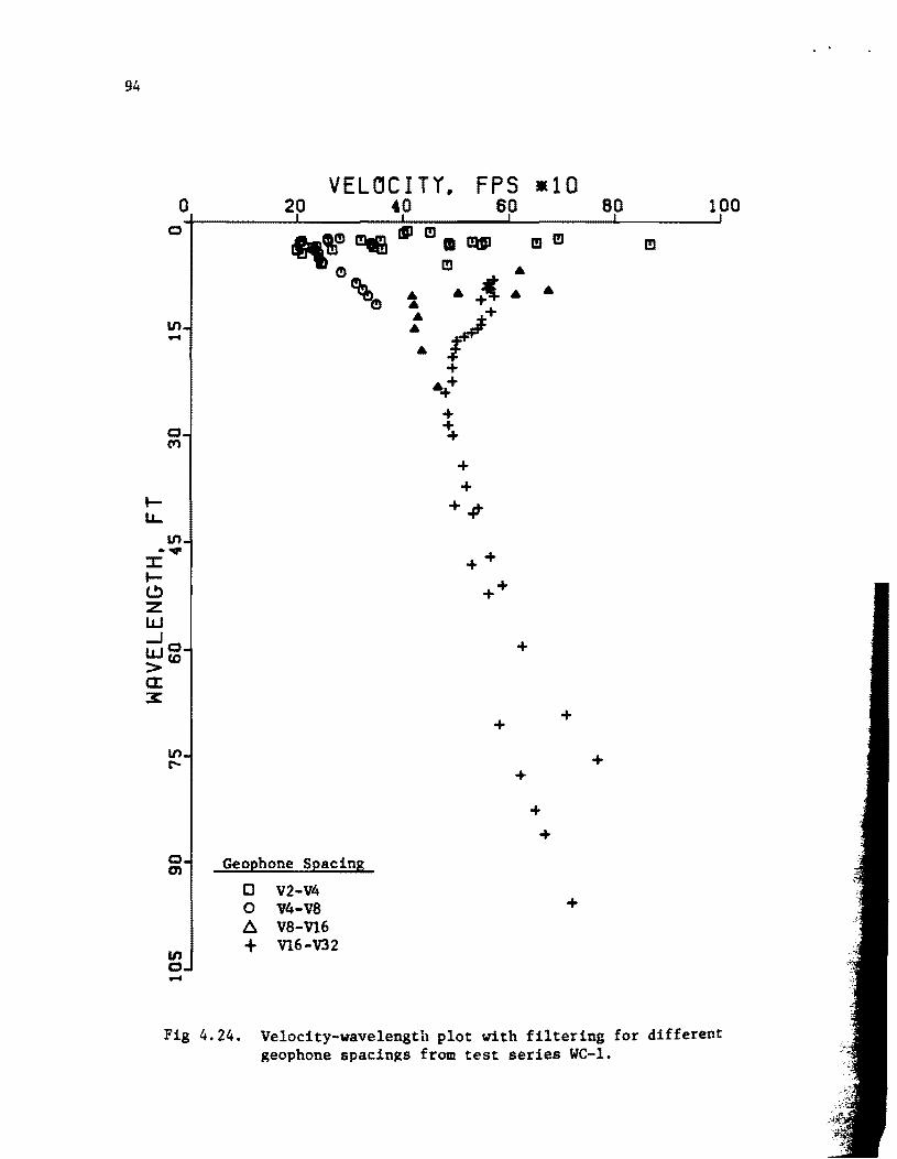
94
VELOCITY. FPS -10 o 20 to 60 80 100
c
lt) ....
+ +
f- +# u... lt) ....
++ :I: f-
++ (!) Z LIJ ...J c + LlJc.o > a: 3:
+ +
II) + E"'" +
+ +
c Geophone Spacing en 0 V2-V4 0 V4-V8 + 6 V8-V16
lt) + V16-V32 c -Fig 4.24. Velocity-wavelength plot with filtering for different
geophone spacin~s from test series We-I.
•
95
In addition to spacing ~ x, the appropriate location of the first
geophone from the source must be considered. Intuitively, the first geophone
should be located at a distance equal to or greater than the particular
wavelength to be measured. This permits ample time for the wave to propagate
due to the influence of the depth to be sampled. In actual field testing, it
is difficult to assess how rigorously this criterion should be followed.
Certainly the first geophone should be spaced some distance away so that any
body wave energy will have had sufficient opportunity to dissipate and, thus,
a wave pulse that is more nearly pure Rayleigh wave energy will be captured.
For that reason, the use of a reference geophone near the source is not
desirable.
This distance also allows more time for the various frequencies
(wavelengths) in the pulse to separate, which should enhance the ability of
the spectral analyzer to transform accurately the wave pulse into its
frequency spectrum. Based on the data in Tables 4.3 and 4.4, the location of
the first geophone is important. For measurements where the far geophone was
located at the same distance in both test series, a greater range of useful 2
frequencies was obtained (based on Y ~ 0.90) when the near geophone was
located away from the source as opposed to being at the reference location
V2. For example, measurement V8-V16 provided data up to 207 Hz while
measurement V2-V16 provided data only up to 87 Hz. It appears that the
"extra" distance from the source to the near geophone provides for a better
overall measurement.
Measurements from Test Series WC-l and WC-2 can be used to test this
hypothesis. Recall that, for Test Series WC-I, both geophones were spaced at
increasing distances from the source, while, for Test Series WC-2, the near
geophone remained at a distance 2 ft (0.6 m) from the source and only the far

96
geophone was moved. Figures 4.22 and 4.23 are replotted in Fig 4.25 to
compare the velocity profiles obtained by the different spacing arrangements.
The profiles begin to diverge at a wavelength of about 60 ft (18 m),
indicating that longer wavelengths are affected more by the difference in
geophone location. Further conclusions can be drawn by comparing the
profiles with shear wave velocities from crosshole tests.
SHEAR WAVE VELOCITY PROFILE
One of the main purposes of dynamic testing in the field is to determine
in situ shear moduli based on measured shear wave velocities. The variation
of modulus with depth can be conveniently described by the profile of the
shear wave velocity versus depth. Heretofore in this chapter, only Rayleigh
wave velocities have been discussed or plotted. Rayleigh wave velocities can
be converted to shear wave velocities 1f the Poisson's ratio of the material
is known or if it can be reasonably assumed.
Before developing and presenting a shear wave velocity profile from
Rayleigh wave velocities, it is necessary to determine a Poisson's ratto (or
several, if material properties vary significantly) for the site. Data from
crosshole tests (ratios of VS/Vp) can be used to calculate an estimate of
Poisson's ratio.
Crosshole Test Results
The crosshole data presented herein were collected and presented by
Patel (Ref 20). The crosshole shear wave velocity profile obtained by Patel
is shown in Fig 4.26. This profile includes measure.ents .ade between

..... u..
a o
U") -o (r)
U") •• ::x::: ..... l!) z UJ -.J o UJ(D > a: ~
o 0)
U") o -
VEL~CIT,,(, FPS -10 20 40 60
o Test o Test
III (!j!J.. .. l!J
~ l!J I!J
-- I!J, I!J I!J
Series WC-l Series WC-2
~~t \ '" 1f1!J~
(!) (!)
(!)
I!JII (!)l!J
l!J (!)
(!)(!)
(!) I!J
(!)
(!)(!)
(!)
I!J
l!J
I!J
I!J
I!J
I!J
80 100
~ (!)
Fig 4.25. Comparison of filtered velocity-wavelength plots for geophone spacings of test series WC-l and WC-2.
97

98
Borehol. and Sourc. Locations
S30nd SI 82 S2 83 54 84 O~------~------~--------~----------~--~-----r~
~oo
5~O
~ -~
~
• g
2
~100
Vii. f~
100
30 0 10 20
D Istlnel t ft
Fig 4.26. Crosshole shear wave velocity profile at Walnut Creek site (Ref 20).

99
boreholes B1 and B5 as depicted in Figs 4.4 and 4.6. A rather large
variation in shear wave velocities exists from borehole to borehole,
particularly at depths from about 15 to 20 ft (4.6 to 6.1 m) •
Table 4.5 contains a summary of the S-wave and P-wave velocities
(average values) obtained by Patel. Above 30 ft (9 m) the degree of
saturation is less than 99 percent, so that these velocities represent
properties of the soil skeleton. The ratio of Vs/Vp was calculated, ard,
using Table 2.1, Poisson's ratios were estimated. Finally, ratios of VR/v S
listed in Table 4.5 were approximated on the basis of Poisson's ratios. At
the Walnut Creek site, Poisson's ratios ranged from 0.31 to 0.40. The ratio
of the Rayleigh wave velocity to the shear wave velocity only varies from
about 0.93 to 0.94. For purposes of analysis, the value of VR/vSwas assumed
to be 0.94 over the entire profile.
Velocity Profile from Cross Spectrum Measurements
Previous discussion of sources showed the sledge-hammer-on-concrete
source provided the best combination of magnitude and coupling to generate
predominantly Rayleigh-wave energy over the range of wavelengths needed to
sample the Walnut Creek site. The velocities plotted in Fig 4.25 as
representative of Test Series WC-2 included only cross spectrum measurements
made with the sledge-haBmer-on-concrete source. The velocities are assumed
to be Rayleigh wave velocities. Using the ratio of VR/Vs equal to 0.94, the
c8lculated R-wave velocities can be converted to S-wave velocities by

100
Depth
(ft)
3
6
9
12
15
18
21
24
27
30
TABLE 4.5. SUMMARY OF CROSSHOL~ T~ST RESULTS AT WALNUT CREEK (REF 20)
S-Wave P-Wave Velocity Velocity Poisson's Vs(fps)* Vp(fps)* VS/Vp Ratio··
540 1248 0.433 0.38
565 1225 0.461 0.36
680 1670 0.407 0.40
735 1775 0.414 0.40
765 1657 0.462 0.36
745 1417 0.526 0.31
730 1415 0.516 0.32
705 1667 0.423 0.39
665 1610 0.413 0.40
640 4883 (Water Table) -I
* S-wave velocities and P-wave velocities from Patel (1981).
** Poisson's ratios and VR/Vs based on VS/Vp using Table 2.1.
· .
VR/VS **
0.94
0.94
0.94
0.94
0.94
0.93
0.93
0.94
0.94
-
101
To obtain a profile of velocity versus depth, some criterion must be
selected regarding the "effective sampling depth" of a given wavelength. The
velocity versus magnitude plot shown in Fig 4.25 can, thereby, be translated
into a velocity versus depth profile. Three such profiles (from measurements
for Test Series WC-l), employing LR/2, L
R/3, and LR/4 criteria, are plotted
together in Fig 4.27. Naturally, the profile using the greatest fraction of
wavelength (L /2) will provide the deepest region of sampling or testing. R
It should be emphasized that the use of a depth criterion based on
wavelength is somewhat empirical. In general, a unique criterion is probably
not correct for all wavelengths. A more accurate solution based on rigorous
theory and numerical analysis is beyond the scope of this study. However,
for typical sites and material properties, the use of a depth criterion based
on wavelength appears to be satisfactory for engineering applications.
Comparisons Between Cross Spectrum Measurements and Crosshole Results
A comparison between cross spectrum measurements and crosshole
measurements serves two purposes. First, it provides a basis for determining
which wavelength criterion (shown in Fig 4.27) yields the most representative
sampling depth at this particular site. Second, it permits a judgement on
the overall ability of a surface measurement to define the shear wave
velocity profile accurately.
The range of values of shear wave velocities (Ref 20) obtained at 3-ft
(0.9-m) intervals to a depth of 30 ft (9 m) is graphed as a band in Fig 4.27.
Based on this band, the shear wave velocity profile increases linearly from
the surface to about 12 ft (3.7 m), remains relatively constant from about 12

VELGCITT. FPS -10 o 20 40 10 10 100 a I ' ~ __ c t , •
•
~.
~.
~-
~ ~
L "'. ON
51
III
•
¥--• , . • • •
- ..
• • • •
-(a) Effective Depth - ~/2
•
VELOCITY. FPS -10 o 20 40 10 10 100
.. \ '¥. .. ~ .... ~ •• ' - '
•
~.
~-
£ ... IL w. ON
I
.,
•
•
(b) Effective Depth a ~/3
VELOCITY. FPS -10 ... 20 40 10 10 100
.. I '-.II! ~"<i" .. ' · ' •
.... ~ .. £ ... IL w. ON
,
-,
Range of Vs from cro8shole tests by Patel (1981)
(c) Effective Depth - ~/4
Fig 4.27. Comparison of various "Effective Sampling Depth" criteria with crosshole results.
I-' o N
. J' ~
~
103
to 21 ft (3.7 to 6.4 m), and then decreases slightly from about 21 to 30 ft
(6.4 to 9.1 m).
If the near-surface and deepest cross spectrum measurements are ignored,
the remaining cross spectrum measurements exhibit a similar trend to the
crosshole results. The profile increases linearly with depth up to a certain
point and then remains relatively constant. The exact depths where the
profile changes depends, of course, on the fraction of wavelength equated to
the effective sampling depth. It appears that most of the cross spectrum
measurements are reflecting the shear wave velocity profile, although, in
most cases, the velocities are lower than velocities obtained from crosshole
tests. On the average, the velocities from cross spectrum measurements are
10 to 20 percent lower than velocities from crosshole tests.
Which wavelength fraction best fits or approaches the crosshole data is
not evident in Fig 4.27. At depths from 0 to 10 ft (0 to 3 m), the LR/4
criterion seems to provide the best agreement with the crosshole profile; at
depths from 10 to 20 ft(3 to 6 m), the LR/3 criterion seems to agree best; at
depths from 20 to 30 ft (6 to 9 m), the LR/2 criterion seems to agree best.
However, there is no apparent theoretical basis for varying the depth of
sampling with wavelength or frequency. Overall, the LR/3 criterion seems to
agree best from 0 to 30 ft (0 to 9 m).
Using the LR/3 criterion, profiles from Test Series WC-1 and WC-2 are
compared with crosshole results in Fig 4.28. The profiles are similar,
although at depths below about 20 ft (0.6 m) the profile from Test Series
WC-2 more nearly approaches the profile obtained from crosshole tests. This
result again suggests that better data are obtained by spacing the near
geophone at a significant distance from the source (as opposed to using the
reference geophone for all measurements).

104
SHEAR WAVE VELOCITY, FPS X 10 o
e
e ....
1-11) u... ....
• :I: Ia.. We ON
If) N
20
~ 0 Test Series WC-l o Test Series WC-2
Effective Depth • LR/3
60
e, e' cfm~
e e
19-em 19
e e e m
e
eo 100
em
19
Range of Vs from crosshole tests by Patel (1981)
19
19
Fig 4.28. Comparison of crosshole results with shear wave velocity profiles obtained from measurements of test series WC-l and test series WC-2.
j -·lS
IDS
In general, velocities from cross spectrum measurements were lower (by
about 10 to 20 percent) than velocities obtained from crosshole tests. For
engineering purposes, this difference is usually not significant. Some
variation may have been due to different moisture conditions, since the two
sets of measurements were performed at different times. Also, since the
cross spectrum measurements use surface receivers, velocities determined at
the greater depths will include an average of lower velocity material nearer
the surface as well as deeper, higher velocity material. The overall effect
of this averaging will probably yield a velocity which is somewhat lower than
the velocity obtained at a specific depth using crosshole tests. The amount
of variation caused by averaging will probably differ slightly from site to
site, depending on the soil properties. Nevertheless, the surface (cross
spectrum) measurements seem to provide a fairly accurate profile of the shear
wave velocity.
ATTENUATION MEASUREMENTS
During both series of tests, transfer function measurements were
recorded. The magnitude of the transfer function gives a ratio of output
energy per given input energy at each frequency. The ratio provided a
measure of the attenuation properties at the site as a function of frequency.
Both geometric damping and material damping were included in the transfer
function, thus supplying data to calculate a coefficient of attenuation, a •
Measurements made during Test Series WC-l contained excessive scatter.
Transfer functions for these measurements are shown in Fig 4.29a. In some
instances, the spectrum from the farther seophone yielded amplitudes greater
than those at the closer geophone (indicated by a transfer function magnitude

106
2.0
-0:: « -c 0 ... (,) C ::J LL. ... G) -., c 0 '-.-
0.0
0
Measurement
-+V2-V4 ...... V4 - va - va- VIS --- VIS- V32
Frequency t Hz
.' . . . . . . : ~ . . . . . ':.
.* *. .... . ..
(8) Test Series WC-1
. . .
100
I.O-r---...-...--------------------------------------------...----------------------~
-0:: « -c 0 -u C ::J
LL.
... G) -." C
e ~
0.0
Measurement
+-+V2-V4 ....... V2- va -V2-VIS ----V2 .. V32 ... ."....,.. .......
~ .,.""" _lIf ... ( .. - .. -+-+-+ \.
".;., ~-.. .. _.... .,. .t'"
~ I ~"'~ ~ v .- ..... ..,. ..... . ......... . \j I·- •• -.- •• • .- * •• . ,.- ... ~ :t* -.. .* ••••• e. ....
0 Frequenc Y. Hz
(b) Test Series WC-2
Fig. 4.29. Comparison of Transfer Function Magnitudes from Different Geophone Spacing Arrangements.
100
..

I 107
greater than unity). In various other cases, the amplitude decay was not
sufficient to account for geometric damping, let alone material damping.
Perhaps the cause of the extreme scatter was the variation of spacing between
the source and the first geophone. As such, different amounts of attenuation
occurred before the wave even reached the first geophone.
During Test Series WC-2, the first geophone was fixed at a location 2 ft
(0.6 m) from the source and only the far geophone was moved to vary the
spacing between geophones. Transfer functions for these measurements are
shown in Fig 4.29b. As a result, there was considerably less scatter in the
data. Meaningful attenuation calculations were possible, although some
scatter did exist. It should be emphasized that the geophone arrangement for
Test Series WC-2 (reference geophone) provided better data for calculation of
attenuation than the geophone arrangement for Test Series WC-1 (equally
spaced geophones), although the latter arrangement was better for determining
the velocity profile.
The output/input'ratios, hereafter referred to as amplitude ratios (AR),
from various transfer functions are summarized in Table 4.6. The transfer
functions represent measurements performed with the sledge-hammer-on-concrete
source (to standardize the source) and over a measurement bandwidth of 100 Hz
(to keep the resolution constant). Amplitude ratios are listed as a function
of spacing (ranging from 2 to 30 ft) and as a function of frequency (6 to
100 Hz).
To compare graphically the attenuation as a function of frequency, it is
necessary to establish some type of datum at which each frequency has the
same initial magnitude. The reference geophone V2 is the most convenient
initial point since it served as the input geopbone for each measurement.
However, the amount of input energy of the sledge-hammer-on-concrete source
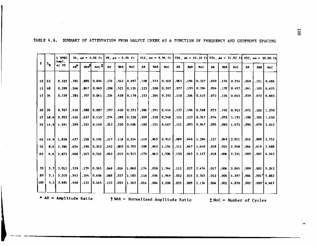
TABLE 4.6. SUMMARY OF ATTENUATION FROlf WAU,'UT CREEK AS A FUNCTION OF FREQUENCY AND GEOPHONE SPACING
L SPEC V4, OX - 2.08 ft va, ox - 6.04 ft V12, ox • 9.94 ft V16, OX • 14.10 ft V24. OX - 21. 92 ft V32, Ax - 30.00 ft
f La A_pI. at V2 A~ MAR1 Nocl AR MAR NoC AR MAR NoC AR MAR NoC AR MAR MoC AR MAR MoC
10 62 0.325 .286 .880 0.034 .176 .542 0.097 .108 .332 0.160 .063 .194 0.227 .050 .154 0.354 .049 .151 0.484
12 48 0.399 .346 .867 0.043 .208 .521 0.126 .123 .308 0.207 .077 .193 0.294 .054 .135 0.457 .041 .103 0.625
15 34 0.539 .381 .707 0.061 .236 .438 0.178 .153 .284 0.292 .110 .204 0.415 .072 .134 0.645 .039 .072 0.882
20 24 0.707 .416 .588 0.087 .297 .420 0.252 .206 .291 0.414 .137 .194 0.588 .073 .103 0.913 .072 .102 1.250
25 18.4 0.952 .416 .437 0.113 .274 .288 0.328 .209 .220 0.540 .121 .127 0.767 .074 .078 1.191 .100 .105 1.630
30 14.9 1.191 .399 .335 0.140 .262 .220 0.406 .180 .151 0.667 .111 .093 0.947 .095 .080 1.471 .094 .079 2.013
40 10.9 1.838 .437 .238 0.191 .217 .118 0.554 .119 .065 0.912 .089 .048 1.294 .127 .069 2.011 .016 .009 2.752
50 8.6 2.384 .454 .190 0.242 .142 .060 0.703 .IOB .045 1.156 .111 .047 1.640 .058 .024 2.548 .046 .019 3.488
60 6.6 2.873 .468 .163 0.316 .042 .015 0.915 .179 .062 1.506 .130 .045 2.137 .018 .006 3.321 .009 .003 4.545
70 5.7 3.012 .539 .179 0.365 .048 .016 1.060 .174 .058 1.744 .112 .037 2.474 .017 .006 3.845 .009 .003 5.263
80 5.1 3.310 .543 .164 0.408 .088 .027 1.185 .118 .036 1.949 .052 .016 2.765 .012 .004 4.297 .004 .001+ 5.882
100 4.5 3.684 .448 .122 0.463 .122 .033 1.343 .014 .004 2.208 .033 .009 3.134 .004 .001 4.870 .002- .000+ 6.667
* AR - Amplitude Ratio t NAR :: Normalized Amplitude Ratio t NoC :: Number of Cycles
I-' o 00

109
was not equal for each frequency (see Fig 4.16b). The amplitude of the wave
energy as a function of frequency can be obtained from the spectrum of V2.
The values of amplitude at V2 for selected frequencies are listed in
Table 4.6. For the sake of comparison, all amplitudes are assumed to equal
unity at V2. To "normalize" the amplitude ratios at other distances, each
ratio must be divided by the spectrum amplitude at the particular frequency.
These normalized ratios are listed in Table 4.6, and, in effect, represent
the amplitudes at the output geophones (V4, VB, etc.) that would have been
measured if all frequencies had been given the same input energy.
The assumption that all amplitudes equal 1.0 at V2 is arbitrary. The
normalized amplitude ratio (NAR) is not an absolute amplitude but serves only
as a relative value to compare attenuation of different frequencies from a
common origin. Ideally, it is desirable to measure input amplitudes at
exactly the source point. Practical experimental limitations preclude the
gathering of attenuation data in this fashion.
Values of NAR are plotted as a function of distance from the source in
Fig 4.30. Also included are
attenuation of Rayleigh waves for
several curves representing amplitude -1
ranging from 0 to 0.25 ft Note that
these curves originate from NAR - 1.0 at 2 ft. For clarity, only selected
frequencies from Table 4.6 are shown. Sufficient scatter exists in the data
to make it not possible to fit a specific attenuation curve to a given
frequency. However, a general trend can be observed. As the frequency
increases, the NAR shows more rapid decrease with distance. This trend is
most clearly illustrated at a distance of 24 ft (measurement V2-V24). This
behavior is not unexpected, since higher frequencies will have undergone more
wavelengths (cycles) to reach a given distance.
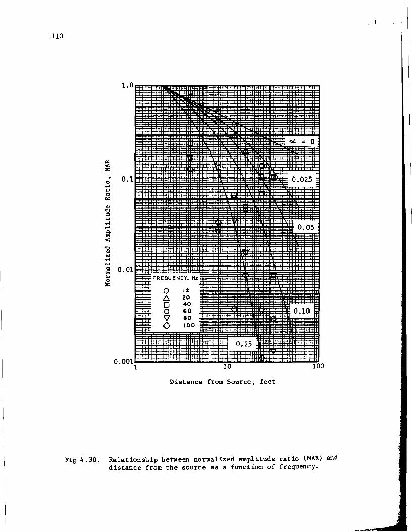
llO
1.0 • II
• 0( = 0
a: ~ ~ 0.1 0.025 0 ~
+J C\l a: ClJ
"tI :I +J ~ .... 0.05 0-E < "tI
ClJ N ~ .... ~ 0.01 ,., lifREQUENCY, ... 0 z
. 0 It
~ 6 20 I 8 :~ 0.10 \l 80
I:::;: <> 100
0.25
0.001 1'00 1 10
Distance from Source, feet
Fig 4.30. Relationship between normalized amplitude ratio (NAR) and distance from the source as a function of frequency.

I . 111
The number of cycles or fractions thereof that a given frequency has
undergone in a given distance can be calculated by
Number of Cycles = ~x/LR (4.7)
Calculations using Eq 4.7 are summarized in Table 4.6. Values of NAR are
plotted as a function of number of cycles in Fig 4.31. Although some scatter
still exists, it appears that all frequencies exhibit similar damping of wave
energy when plotted as a function of number of cycles. This suggests that
the material damping is independent of frequency (at least over the range of
frequencies observed in these measurements).
The expression for R-wave attenuation (in a homogeneous, isotopic
half-space) which includes both geometric and material damping was given in
Chapter 2 as follows:
A2 til [ ~ AR = -- = -- exp -a(r - r ) Al r 2 2 1
(4.8)
Rearranging terms to evaluate a , when all other variables are known, yields
a = (4.9)
where a has dimensions of l/distance and the same units as rl and r2.
Equation 4.9 was used to calculate values of a as a function of frequency.
Values of -1 1 ranged from 0.031 ft to 0.435 ft-, with the larger values
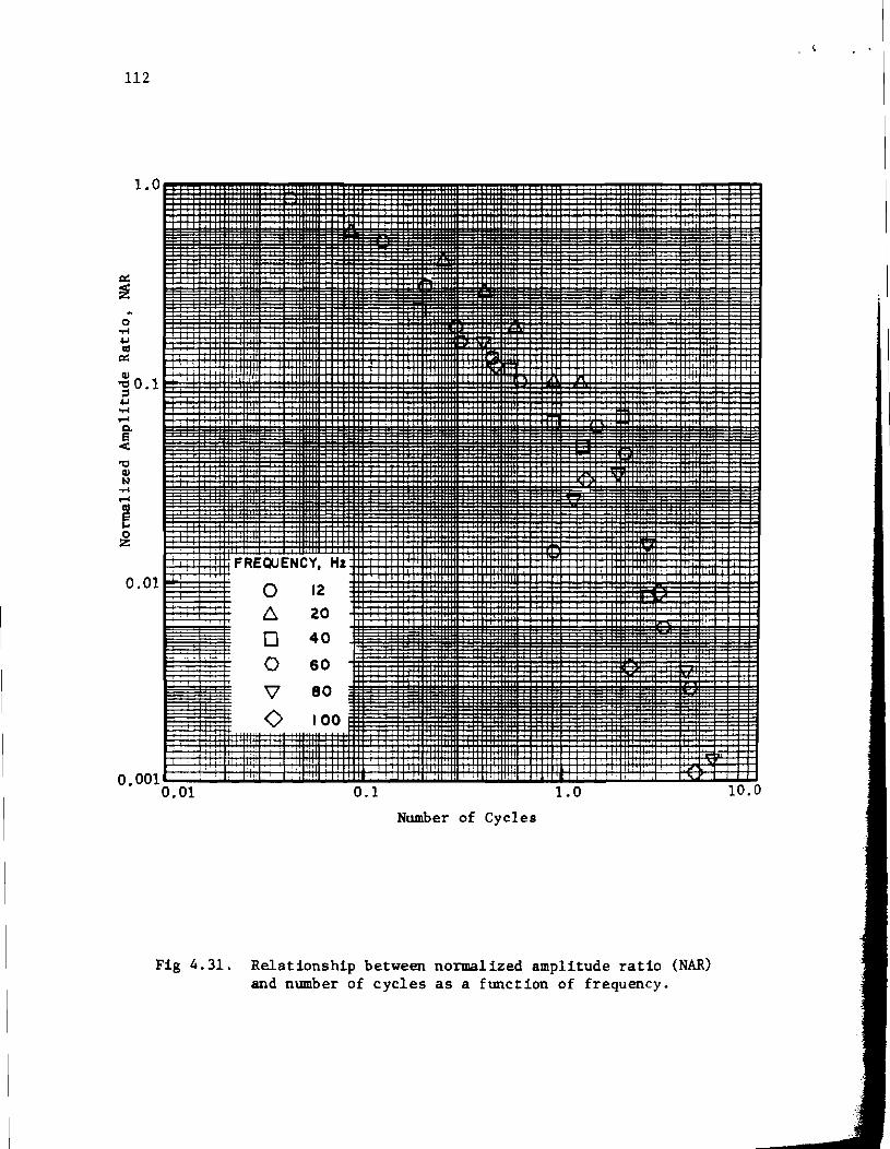
112
~
o ~ 4.1 III
ex: Cl.I ] 0.1 4.1 ~ r-I 0-S < '0
Cl.I N ~ r-I
E o z
0.01
0.001 0.01
FREQUENCY, Hz
o 12
6 20
o 40
o 60
'V 80
o 100
0.1 1.0
Number of Cycles
Fig 4.31. Relationship between normalized amplitude ratio (NAR) and number of cycles as a function of frequency.
10.0

I I •
113
resulting from measurements V2-V4 and V2-VS where the waves had undergone
only a small fraction of a cycle. Much of the scatter is reduced if values
of are calculated only for waves that have travelled at least one-third of
their wavelength at a given geophone location.
Using this criterion, the range in as a function of frequency is
shown in Fig 4.32. Average values are indicated by the solid circles.
Figure 4.32 shows that increases with frequency. This graph more clearly
illustrates the trend observed in Fig 4.29. A linear regression analysis
performed with the average values plotted in Fig 4.31 indicates the a is
very nearly a linear function of frequency. A correlation coefficient of
0.97 was obtained for a line with a slope of 0.00173. Due to slight scatter
in the data, a small intercept value was also obtained, although,
theoretically, as f approaches zero (L approaches infinity), no attenuation R
should occur and a should equal zero.
The relationship a • 0.00173 f was used to calculate values for a that
did not exhibit the general scatter in the measured values of a. In
addition, values of the logarithmic decrement 0 and damping ratio D were
calculated using the equations presented in Chapter 2. Each of these
quantities is listed in Table 4.7.
The values of damping ratio (expressed as a percentage) do not vary
significantly with frequency. This confirms the conclusion that was drawn
from Fig 4.30, namely, that material damping 1s independent of frequency over
the range from 0 to 100 Hz. Damping values ranging from about 11 to 17
percent are somewhat higher than those typically measured in the laboratory.
There are at least two possible explanations for this discrepancy. First, it
is possible that significant body wave energy was still present in the wave
pulse at the reference geophone (V2). This energy would have dissipated due

114
t""4 I ~ ~
7 ........
c 0 .... ~
III =' C Q)
~ ~
< ~ 0
~ c Q) .... 0 .... ~ ~
Q)
0 u
0.5 ~------~------~~------~--------~------~-
0.4
Range
0.3
0.2
0.1
II ill i 0.0
0 20 40 60 80 100
Frequency. Hz
Fig 4.32. Variation of coefficient of attenuation with frequency at Walnut Creek site.
, \

TABLE 4.7. RELATIONSHIP BETWEEN FREQUENCY AND DAMPING AT WALNUT CREEK SITE.
Coefficient Logarithmic Damping Frequency Wavelength of Decrement Ratio
Attenuation f(Hz) LR(ft) a(ft-1 ) ti D('7.)
10 62 0.017 1.07 16.8
12 48 0.021 1.00 15.7
15 34 0.026 0.88 13.9
20 24 0.035 0.83 13.1
25 18.4 0.043 0.80 12,6
30 14.9 0.052 0.77 12.2
40 10.9 0.069 0.75 11.9
50 8.6 0.087 0.74 11.7
60 6.6 0.104 0.69 10.9
70 5.7 0.121 0.69 10.9
80 5.1 0.138 0.71 11.2
100 4.5 0.173 0.78 12.3
115

...
116
to geometric damping at a greater rate than the surface wave energy by the
time the wave pulse reached the far geophone. As a result, the far geophone
would have interpreted some of the geometric damping of the body wave as
material damping of the Rayleigh wave, thus yielding an erroneously high
value for a. The other possible explanation is that the higher damping
values are true properties of the in situ material. Factors such as
non-homogeneities or reflection and refraction of wave energy due to layering
may cause "backscattering" which yields a field damping that is somewhat
higher than that measured in the laboratory sample.
It appears that attenuation, or damping, can be measured in the field
with the use of the transfer function. Based on results at the Walnut Creek
site, better attenuation data can be obtained by using a fixed reference
geophone than by using an equally spaced arrangement of geophones. However,
before such data can be used with confidence, the problems cited above should
be resolved.
SUMMARY
Results and conclusions based on tests performed at Walnut Creek can be
categorized in terms of measurement set-up, type of source, interpretation of
velocity profile, and determination of damping.
In general, measurements made with five averages (transient events) will
provide reliable data. Additional averages in the measurement are Dot
warranted because they do not significantly improve the data. Frequency
resolution is not a problem if the frequency bandwidth is commensurate with
the geophone spacing. Close spacings near the source may use a higher
frequency range (100 Hz to perhaps 800 Hz) while wide spacings farther frOi
.'

I . 117
~ -
i the source should use a lower frequency range (25 to 100 HZ). Selection of a
lower (narrower) frequency bandwidth will provide better resolution of long
wavelengths needed to sample greater depths.
A source should be used which generates predominantly Rayleigh wave
energy and minimizes body wave energy in the wave pulse. A vertical blow
from a hammer which is in direct contact with the soil a good source. The
magnitude of the input energy does not seem to be a critical factor as long
as adequate energy is provided to excite low frequencies. The coupling of
the source with the soil, which influences the transfer of energy, is an
important factor. In this regard, the use of a plate between the hammer and
soil should be avoided.
The velocity profile obtained from surface measurements will probably
have some scatter. Better measurements can be obtained when the geophones
are appropriately located from the source. Based on results at Walnut Creek,
a spacing arrangement in which the first geophone is located at increasing
distance from the source is more favorable than an arrangement In which the
first geophone is fixed at a reference location close to the source. In
addition, much of the scatter in the velocity profile can be reduced by
filtering out data for wavelengths which are inappropriate for the spacing of
the geophones. Wavelengths which are too short for a given spacing may
attenuate excessively, whereas wavelengths which are too long for a given
spacing may not have travelled a sufficient distance to sample adequately the
depth proportional to the wavelength. Using the criteria discussed in this
chapter, an appropriate range of LR for a given spacing ~x was found to be
(4.10)

118
Equation 4.10 was used to filter inappropriate wavelengths which resulted in
a refined velocity profile.
The velocity profile obtained from cross spectrum measurements was
compared with velocities from crosshole tests by applying depth criteria of
LR/4, L
R/3, and LR/2. The comparison of profiles did not clearly indicate
which depth criterion is most appropriate for surface measurements. Overall.
the velocities plotted at a depth of ~/3 appeared to correlate well with the
crosshole velocities. On the average, the cross spectrum velocities were 10
to 20 percent lower than the crosshole velocities. However, this difference
is considered tolerable for practical engineering applications.
Attenuation properties at the site were evaluated by means of transfer
functions. The coefficient of attenuation a was found to be approximately a
linear function of frequency and was estimated by a - 0.00173 f. Values of
logarithmic decrement and damping ratio were also calculated. Damping ranged
from about 11 to 17 percent. These values are somewhat higher than those
typically measured in the lab, possibly due to backscattering of wave energy
caused by reflection from layer boundaries or anamolies at the site. or
because there is excessive body energy at the near geophone which is located
relatively close to the source.

CHAPTER 5. SOIL TESTING AT THE CROSSING SITE
SITE DESCRIPTION
The second soil site at which R-wave dispersion testing was performed
was the Crossing site. The Crossing site is located about 4 miles (6.4 km)
southeast of the campus of The University of Texas at Austin, as shown io
Fig 5.1. The site is part of an open tract of land currently undergoing
development. The actual test area is located about 1000 ft (300 m) from the
city street (East Riverside Drive). Because the site is open and away from
traffic, ambient noise at the site is minimal.
The site lies in the flood plain of the Colorado River, and, as a
result, the topography of the site is relatively flat. The soil profile
consists of a medium dark clay deposit underlain by sand. The clay extends
to a depth of approximately 30 ft (9 m). During dry periods, the soil within
a few feet of the surface becomes highly desiccated and undergoes extensive
shrinkage cracking.
Because the site is not located near any structures, power to operate
electrical equipment had to be supplied by a portable power generator.
119
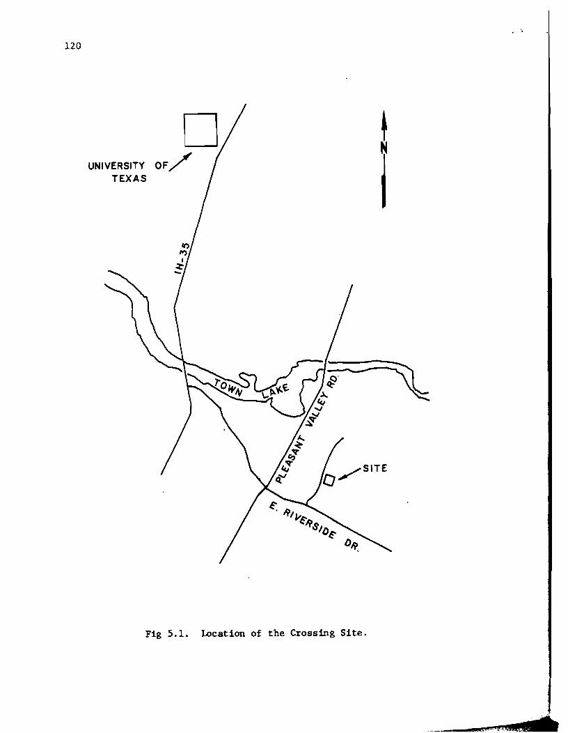
120
UNIVERSITY OF / TEXAS
Fig 5.1. Location of the Crossing Site.
~
I
.«·#4#1& ..
121
EXPERIMENTAL PROCEDURE
Testing at the Crossing site was conducted on May 28, 1981. The soil at
the surface was soft (but not muddy) from heavy rainfall that had occurred
during the previous week. The source used to generate wave energy was the
drop hammer previously described in Section 4.3.1 and illustrated in
Fig 4.7a. The drop hammer was used in direct contact with the soil surface.
Two vertical geophones were used to capture the time domain signal of
the propagated wave. The geophones used at the Crossing were the same as
those used at Walnut Creek for Test Series WC-1. Each geophone had an
undamped natural frequency of about 8 Hz and had a shunt resistance which
provided a damping of approximately 50 percent of critical damping. The
transduction constant was in the range of 1 volt per in./sec (0.4 volt
per cm/sec). The frequency response curves for the two geophones are shown
in Fig 4.3.
The geophones were placed in augured holes to minimize background noise
generated by the wind striking the geophones and to improve the geophone-soil
contact. The holes were augured to a depth of 4 to 6 in. (10.2 to 15.2 cm).
Each geophone was then embedded at the bottom of the hole by means of a steel
spike on the end of the geophone and the remainder of the hole was backfilled
with augured soil.
The locations of the geophones for the various measurements are shown in
Fig 5.2. One set of measurements was performed with the near geophone
located at increasing distance from the source and then spacing the far
geophone at that same distance (source to near geophone) from the near
geophone. In other words, the first geophone was located exactly midway
between the source and the far geophone. (This arrangement is similar to

I ~
approx. 40 ft ~ to curb I 7.85 I 7.90 I 7.87 I
OB4 OB3 OB2 OB1
source,\ 2 4 6 8 10 16 18 26
* n 11 0 6. 0 6. 0 0
• Direction of Wave Propagation
Legend
<=) Existing boreholes used in work performed by Hoar (1981).
o Location of geophones (with distance from source in feet) for measurements with a "reference" geophone at 2 ft.
6. Location of geophones (with distance from source in feet) for measurements with the near geophone located midway between the source and the far geophone.
Fig 5.2. Locations of source and geophones for testing at the Crossing Site.
I-' N
f N
N
j
32 34 6. 0

123
that for test series We-I.) Another set of measurements was performed with a
reference geophone at 2 ft (0.6 m) from the source and with only the far
geophone increasing in distance from the source. (This arrangement is
similar to that for Test Series WC-2.) The location of the far geophone was
selected so that the spacing between geophones was the same as that for
measurements having the equally spaced arrangement.
A summary of the measurements performed at the Crossing is presented in
Table 5.1. Hereafter, these measurements will be identified by the location
of the pair of geophones. For example, measurement V16-V32 identifies the
measurement recorded with the near vertical geophone (V) located at 16 ft
(4.9 m) from the source and the far vertical geophone located at 32 ft
(9.8 m) from the source.
SHEAR WAVE VELOCITY PROFILE
The shear wave velocity profile can be obtained from' Rayleigh wave
velocities if Poisson's ratio is known or assumed. If available, data from
crosshole tests (both P- and S-wave velocities) can be used to calculate an
estimate of Poisson's ratio. One of the reasons for selecting this site is
that crosshole tests had been previously performed there by Hoar (Ref 11).
The shear wave velocities at the site increase from about 500 fps (150 mps)
at the surface to nearly 1000 fps (300 mps) at a depth of 30 ft (9 m).
Values of S-wave and P-wave velocities (obtained by Boar) at 3-ft (O.9-m)
intervals are listed in Table 5.2.
The ratio of VS/Vp was calculated at each depth, and by using Table 2.1,
the corresponding value of Poisson's ratio was determined. Then ratios of
V Iv were determined using Poisson's ratios. R S
Table 5.2 contains each of

TABLE 5.1. SUMMARY OF MEASUREMENTS AT THE CROSSING SITE
Record No. Diet.nce frOID Distance Source Number Bandwidth (Track No.) Source to between of of
Geophones (ft) Geopbones Averagea Spectrum
Near Far (ft) (Hz)
9(1) 2.0 4.0 1.0 Drop Hammer on SolI 5 1600
14(1) 2.0 4.0 2.0 " .. .. .. 5 200
190) 2.0 6.0 4.0 .. .. II It 5 200
24(1) 2.0 10.0 8.0 It .. .. II 5 200
29ft) 2.0 18.0 16.0 .. It " II 5 100
36(1) 2.0 26.0 24.0 " " It It 5 100
41(1 ) 2.0 34.0 32.0 It If It If 5 100
42(1) 2.0 34.0 32.0 .. " .. II 5 25
48(1) 4.0 8.0 4.0 " It II It 5 200
53(1) 8.0 16.0 8.0 II It It It 5 100
58(1) 16.0 32.0 16.0 It It .. " 5 100
59(1) 16.0 32.0 16.0 It It " It 5 25 -
~
Computer Data File
Ident Uication
SHCROI
SHCR02
SHCR03
SHCR04
SHCR05
SHCR06
SHCR07
-SIICR08
SHCR09
SHCRI0
SHCRll
..... N J:'-

· .
Depth
(ft)
3
6
9
12
15
18
21
25
30
TABLE 5.2. SUMMARY OF CROSSHOLE TEST RESULTS AT THE CROSSING SITE (FROM HOAR, 1981)
S-Wave P-Wave Velocity Velocity Poisson's
VS(fps)* Vp(fps)* VS/Vp Ratio**
509 1568 0.325 0.44
577 1611 0.358 0.43
636 1985 0.320 0.44
650 2008 0.324 0.44
689 2064 0.334 0.44
699 2146 0.326 0.44
666 2218 0.300 0.45
738 2149 0.343 0.43
978 5000 (Water Table) -I
* S-wave velocities and P-wave velocities from Hoar (1981).
** Poisson's ratios and VR!VS based on VS!Vp using Table 2.1.
125
VR!VS**
0.95
0.95
0.95
0.95
0.95
0.95
0.95
0.95
-

126
these ratios for each depth. At the Crossing site, Poisson's ratios range
from 0.43 to 0.45. Over this range, the value of VR!VS is approximately
0.95. Hence, a value of 0.95 was assumed for the entire profile to convert
Rayleigh wave velocities to shear wave velocities.
Velocity Profiles From Cross Spectrum Measurements
As a first approximation, a depth criterion of LR!3 was used to
represent the effective depth at which the R-wave sampled and, hence, the
depth at which the R-wave velocity should be plotted. The relationship
Vs K VR!O.95 was then used to obtain shear wave velocities. Two profiles
were developed using this approach: one using measurements made with the
reference geophone arrangement and one using measurements made with the
equally spaced geophone arrangement.
The S-wave velocity profile obtained using measurements made with the
reference geophone is shown in Fig 5.3. A large amount of scatter exists
over the entire profile, with values of velocity at a given depth varying by
as much as three-fold, depending on which measurement is examined.
Figure 5.4 shows the same profile after the data has been filtered using the
criterion given by Eq 4.5(~~x ~ LR ~ 36x). For the longest spacing
(measurement V2-V34), Eq 4.5 excludes wavelengths above 96 ft (29 m) and
depths below 32 ft (9.8 m). Comparison of Figs 5.3 and 5.4 indicates that
filtering the data eliminates much of the scatter in the profile. However,
significant scatter still exists from about 6 to 9 ft (1.8 to 2.7 m) and
below about 22 ft (6.7 m).
The S-wave velocity profile obtained using measurements with equally
spaced geophones is shown in Fig 5.5. Significant scatter in velocity exists
. '
-~

0 e
e -t-lIl u..-
• :::c t-o.. We ON
III N
VELOC I TY. FPS -10 20 40 60
~1t ... :f: .. m C!) +x •
m m A + .£ Ii " A +X • m A + •
C!) +x • E!J (!) es,B: + X ••
I!J(!)A A+ x. A
Geophone Spacing
o V2-V4 o V2-V6 A V2-VIO + V2-V18 X V2-V26 <> V2-V34
+
+ xx.
.~ • ~
+ ~ . +
'" +
• X
• •
+ X ¥
A
•
80 100
X
+
Fig 5.3. Unfiltered shear wave velocity profile for measurements using a reference geophone located 2 ft from the source.
127

128
• ~ ~ Q..
o e
e -
We ON
\f)
N
VELOC I TY. 20 40
FPS -10 60
Geophone Spacing
o V2-V4 o V2-V6 A V2-VIO + V2-VlS X V2-V26 <> V2-V34
6 +X 6 + ~ 6
6 +X • 6 + • +X •
+X •• + X. + xx.
l • ~
X
• •
• X
• •
X X
•
80 100
X
Fig 5.4. Filtered shear wave velocity profile for measurements using a reference geophone located 2 ft from the source.
. . J .

VELCIC I TY, FPS -10 0 20 40 60 80 100
0
+"-*+. + + • I!! • + • ++ +
I!! HI I!! •• • + I!! • +
I!! (!) • 0 ~ • +
I!! + - • + (!) • + (!)
• + ++ • t-1Il + ++ IL- +
+ • +
:c .f+ t-
Q... + UJo ON
+ •
1Il + N
(!)
Geo2hone Seacins
0 CI V2-V4 + crl 0 V4-V8 6 V8-V16
+ + V16-V32
1Il crl
Fig 5.5. Unfiltered shear wave velocity profile for measurements using an arrangement of equally spaced geophones.
129
+
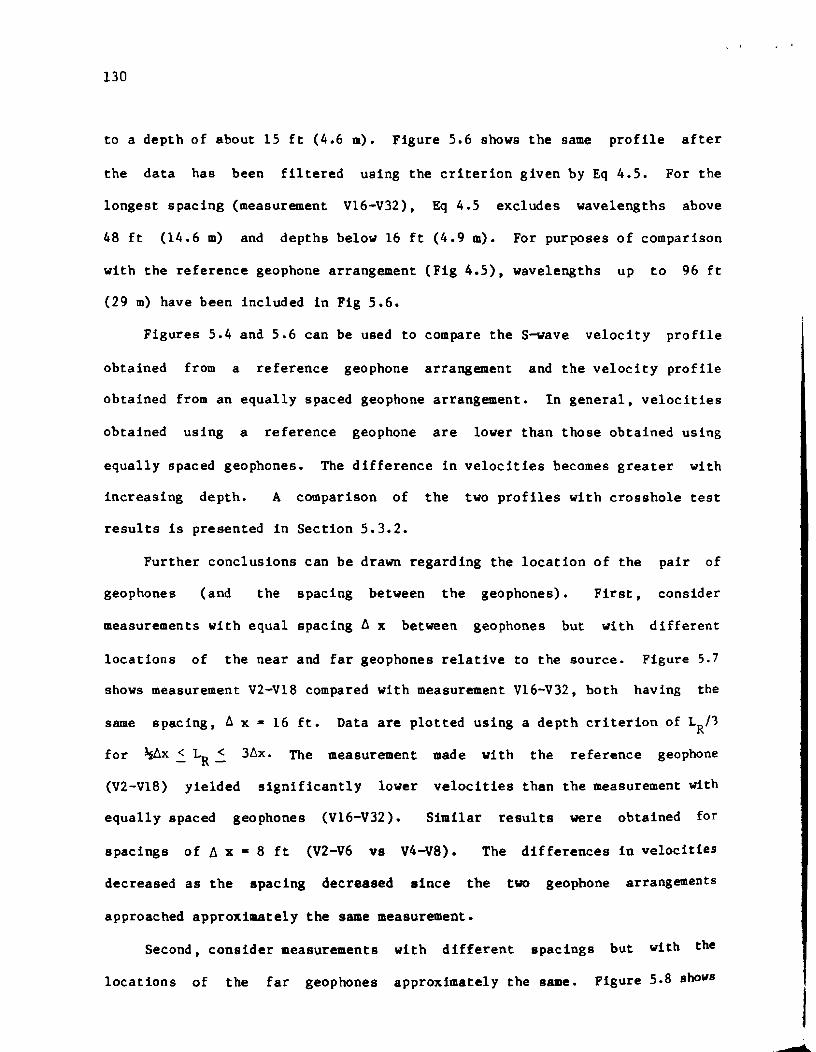
130
to a depth of about 15 ft (4.6 m). Figure 5.6 shows the same profile after
the data has been filtered using the criterion given by Eq 4.5. For the
longest spacing (measurement VI6-V32) , Eq 4.5 excludes wavelengths above
48 ft (14.6 m) and depths below 16 ft (4.9 m). For purposes of comparison
with the reference geophone arrangement (Fig 4.5), wavelengths up to 96 ft
(29 m) have been included in Fig 5.6.
Figures 5.4 and 5.6 can be used to compare the S-wave velocity profile
obtained from a reference geophone arrangement and the velocity profile
obtained from an equally spaced geophone arrangement. In general, velocities
obtained using a reference geophone are lower than those obtained using
equally spaced geophones. The difference in velocities becomes greater with
increasing depth. A comparison of the two profiles with crosshole test
results is presented in Section 5.3.2.
Further conclusions can be drawn regarding the location of the pair of
geophones (and the spacing between the geophones). First, consider
measurements with equal spacing ~ x between geophones but with different
locations of the near and far geophones relative to the source. Figure 5.7
shows measurement V2-V18 compared with measurement VI6-V32, both having the
same spacing, ~ x - 16 ft. Data are plotted using a depth criterion of LR/1
for ~~x ~ LR ~ 3~x. The measurement made with the reference geophone
(V2-VI8) yielded significantly lower velocities than the measurement with
equally spaced geophones (VI6-V32). Similar results were obtained for
spacings of ~ x • 8 ft (V2-V6 vs V4-V8). The differences in velocities
decreased as the spacing decreased since the two geophone arrangements
approached approximately the same measurement.
Second, consider measurements with different spacings but with the
locations of the far geophones approximately the same. Figure 5.8 shows
, '

0 0
0 -1-11) LL.-
• ::I: I-a.. Wo ON
II) N
VELCJC I TY, FPS -10 20 40
""!)U .. C!)eA
Geophone Spacing
o V2-V4 o V4-V8 6. V8-V16 + V16-V32
C!) .. .. .. .... .. ..
60
+
++ .t
+
+
+ + +
+ +
++
+ ++ +
+ +
++ +
80
+
+
Fig 5.6. Filtered shear wave velocity profile for measurements using an arrangement of equally spaced geophones.
131
100
+
+

132
o o
N
...... LLCD
• ::t: ...... CL UJ QeD
0 -
N -
• -
VELClC I TY. 20 40
Measurement
o V2-V18 o V16-V32
l!J I!J
l!J
l!J
l!J
l!J
l!J
l!J
l!J
I!J
l!J
FPS -10 60
(!)(!)
(!)
(!)
(!)
(!) (!)
(!)
80
Fig 5.7. Comparison of reference geophone arrangement with equally spaced geophone arrangement for measurements with similar spacing between geophones.
..
100

-------------
a 0
0 -~lf)
u...-
• :I: ~ CL L&.Jo ON
If)
N
o (I')
20
Measurement
o V2-V34 o V16-V32
VELCJC I T1', FPS -10 40 SO 80
" ~m
(!)(!)
rI m m ~
rtlJm (!)
m (!) (!)
m (!)
lB (!) m (!)(!)
m (!) (!)(!)
m (!) (!) (!)
m ~
m
m
I!l
Fig 5.8. Comparison of reference geophone arrangement with equally spaced geophone arrangement for measurements with similar location of the far geophone.
133
100
(!)
(!)
(!)

134
measurement V2-V34 compared with measurement V16-V32. For each measurement
the distance from the source to the far geophone is nearly equal. Again, the
measurement with the reference geophone (V2-V34) yielded lower velocities
than the measurement with equally spaced geophones (V16-V32).
Since different velocity profiles can be obtained from different
geophone arrangements despite identical spacing 6 x between geophones and
despite a similar location of the far geophone, it can be concluded that the
location of the geophone nearer the source is a significant parameter. One
approach to determine which geophone arrangement provides the better velocity
profile is to compare velocities from cross spectrum measurements with
velocities from crosshole tests. Also, a rational approach incorporating
fundamentals of wave propagation can be considered. Both of these approaches
are presented in the next section.
Comparison Between Cross Spectrum Measurements and Cr08shole Results
The velocity profiles shown in Figs 5.4 and 5.6 are replotted in Fig 5.9
along with the velocity profile from crossho1e test results obtained by Hoar
(Ref 11). The velocities from the cross spectrum measurements have been
adjusted to shear wave velocities and are plotted using a depth criterion of
LR/3. Based on the comparison of velocity profiles in Fig 5.9, it appears
that measurements made using the
correlate significantly better with
equally spaced
the crossho1e
geophone arrangement
resul ts than do the
measurements made using the reference geophone arrangement. This conclusion
is particularly evident at greater depths, where velocities from measurements
made using the reference geophone arrangement are as much as 35 percent lower
than velocities from crosshole tests.
..

VEL~CITY. FPS -10 a 60 80 1
o
I!J
0 I!JI!J - I!J~ , I!J I-I!J e ee u..- e
e .. I!J e ::t: I!J I-0... UJ ON I!J
I!J. e
I!J e
N I!J
o Reference Geophone Arrangement o Equally Spaced Geophone Arrangement
---- Crosshole Velocity Profile (from Hoa~ 1981)
I!J
Fig 5.9. Comparison of crosshole results with shear wave velocity profiles from different geophone arrangements using as "Effective Sampling Depth" of L
R'3.
135

136
A rational approach involving concepts of wave propagation also supports
the use of an equally spaced geophone arrangement. The geophone nearer to
the source should be located at sufficient distance to allow proper sampling
of material to a depth of approximately one wavelength. This distance also
permits wavelengths of different frequencies to separate and enhances the
capability of the spectral analyzer to measure an accurate cross spectrum.
The use of a reference geophone close to the source does not provide
sufficient distance to allow proper sampling to a depth of one wavelength.
As a result, material properties near the surface are overweighted. For most
soil sites, where the velocity (or modulus) increases with depth, the
velocities obtained by using the reference geophone arrangement will be too
low (since the lower-velocity material near the surface was overweighted).
In general, then, the velocity profile obtained with the reference geophone
arrangement will be lower than the actual profile (as determined by crosshole
tests). This conclusion is shown quite clearly in Fig 5.9 for the tests
performed at the Crossing.
The depth criterion of L 13, when applied to measurements made using the R
equally spaced geophone arrangement, provides good correlation with the
crosshole results. In general, the cross spectrum velocities do not vary by
more than 10 percent from the crosshole velocities. Variations near the
surface may be due to seasonal differences in moisture content of the soil.
The cross spectrum measurements were performed a few days after a period of
heavy rainfall, and the lower velocities probably reflect the "softer"
properties of the surficial a011.
A depth criterion of LR/2 was also used to correlate the velocity
profile with the crosshole results. This criterion provided a reasonably
good correlation down to about 20 ft (6.1 m), as shown in Fig 5.10. BeloW

o o
-I-LL.N
.. :t: I-a... LaJN 0""
VELClC I TY, .0
m m
I'm m
8
m m
m l!JI!l
m mm m m
'rF
m
o Cross Spectrum Measurements Crossho1e Results (after Hoar, 1981)
100
m
m
m
Fig 5.10. Comparison of crosshole results with shear wave velocity profile from measurements with equally spaced geophones using a depth criterion of L
R/2.
137

138
this depth, the velocity profile from cross spectrum measurements diverges
markedly from the crosshole results. Inasmuch as crosshole test data exists
only to 30 ft (9 m), it is difficult to assess how well either criterion
(LR
/2 or LR/3) correlates the cross spectrum velocities with crosshole
velocities for depths greater than 30 ft (9 m).
ATTENUATION
Transfer function measurements were used to gather data on the
attenuation properties at the site. The output/input ratio of wave magnitude
(or energy) was obtained as a function of frequency over the range from 10 to
100 Hz. Transfer functions for measurements made using equally spaced
geophones are shown in Fig 5.lla, and the corresponding coherence functions
are shown in Fig 5.l1b. The data exhibits several anomalies such as
output/input ratios greater than unity. In some instances, transfer function
magnitudes for a large spacing between geophones (e.g., V8-V16) are greater
than magnitudes for a shorter spacing (e.g, V4-V8). This behavior is
inconsistent with R-wave attenuation, since measurements with increased
spacing should exhibit decreasing magnitudes. The erratic coherence,
particularly above 45 Hz, also suggests that the transfer functions for
measurements made using equally spaced geophones would not yield reliable
attenuation data.
In contrast. transfer functions for measurements made using a reference
geophone are shown in Fig 5.12a. and the corresponding coherence functions
are shown in Fig 5.l2b. The magnitudes of the transfer functions generally
decrease with increased spacing between geophones. which is consistent with
attenuation behavior. The coherence is also significantly better for
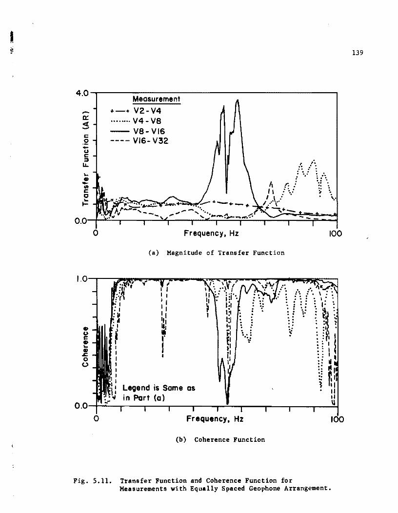
4.0
-0:: « -c .2 -u C :l LL
... 4D -III C C ... t-
0.0
0
I.
Measurement
+-+ V2-V4 ........ V4 - va - va-vIs ---- VIS- V32
Frequency. Hz
. I I. .. . . .. .. . ., .. . . .. . . t' : : ... . .,. .
r. : :: ~ . '. . ) \ 'I..,
100
<a) Magnitude of Transfer Function
. .' f-: .: '. \ : : . . . . " .
I : :: : I: !
~ ~!V ~~~: ~ :: :: ~
~. .:,. ~ -: . . , I • ::,1 I : : I t I '. I ~ : :: I • t :: ~ I :: 111
: LAltend is Same as ~ r: I I -w • II
I I I I II
1,1 · · · "I · · · · ~ · · • 0 · . · .. ,. '0. , ~
-" in Part (0) II O.O-T---.---,----r---r---.-~~--,_--~--_r--~u
o Frequency. Hz
(b) Coherence Function
Fig. 5.11. Transfer Function and Coherence Function for Measurements with Equally Spaced Geophone Arrangement.
139

140
1.0
-0::: <t -c: 0 -0 c: j lL. .... CD -." c: 0 .... ~
0.0
., o c: ., .... ., .c o o
0
.. . , . ,
Frequency, Hz
Measurement
+-+ V2-V4 V2-V6
- V2- VIO ---- V2- VIS
.... . . . ..'"
100
<a) Magnitude of Transfer Function
r
, . . ' ':. If· ','
Legend is Same as in Part (a)
O.O-+----~---~---_,---~r_---~--r_--~--~--~~
o Frequency, Hz
(b) Coherence Function
Fig, 5.12. Transfer Function and Coherence Function for Measurements with Reference Geophone Arrangement,
100
. r
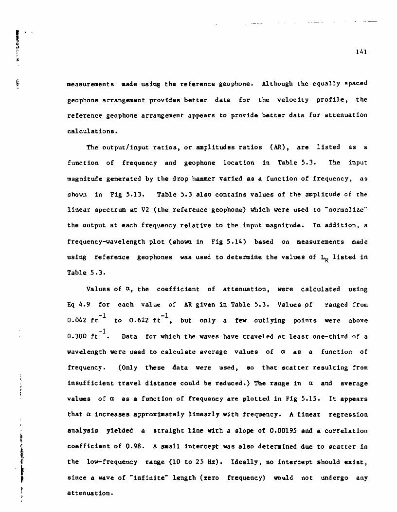
141
measurements made using the reference geophone. Although the equally spaced
geophone arrangement provides better data for the velocity profile, the
reference geophone arrangement appears to provide better data for attenuation
calculations.
The output/input ratios, or amplitudes ratios (AR), are listed as a
function of frequency and geophone location in Table 5.3. The input
magnitude generated by the drop hammer varied as a function of frequency, as
shown in Fig 5.13. Table 5.3 also contains values of the amplitude of the
linear spectrum at V2 (the reference geophone) which were used to "normalize"
the output at each frequency relative to the input magnitude. In addition, a
frequency-wavelength plot (shown in Fig 5.14) based on measurements made
using reference geophones was used to determine the values of ~ listed in
Table 5.3.
Values of a, the coefficient of attenuation, were calculated using
Eq 4.9 for each value of AR given in Table 5.3. Values pf ranged from
0.042 ft-1 to 0.622 ft-1 , but only a few outlying points were above
-1 0.300 ft Data for which the waves have traveled at least one-third of a
wavelength were used to calculate average values of a as a function of
frequency. (Only these data were used, 80 that scatter resulting from
insufficient travel distance could be reduced.) The range in a and average
values of a as a function of frequency are plotted in Fig 5.15. It appears
that a increases approximately linearly with frequency. A linear regression
analY8is yielded a straight line with a slope of 0.00195 and a correlation
coefficient of 0.98. A small intercept was also determined due to scatter in
the low-frequency range (10 to 25 Hz). Ideally, no intercept should exist,
since a wave of "infinite" length (zero frequency) would not undergo any
attenuation.

l
TABLE 5.3. SUMMARY OF ATTE~~ATION FROM THE CROSSING AS A FUNCTION OF FREQUENCY AND GF.OprONE SPACING
L SPEC V4, 6lt - 2.0 ft V6, ~- 4.0 ft VIO, ~ - 8.0 ft VI8, QIl - 16.0 ft V26, QIl - 24.0 ft V34, ~ - 32.0 ft
f ~ Amp I. at V2 AR* HARt NOC* AR HAR NoC AR HAR NoC AR HAR NoC AR HAR NoC AR HAR NoC
10 64 2.693 .542 .2013 0.031 .361 .1341 0.063 .244 .0906 0.125 .082 .0304 0.250 .037 .0137 0.375 .023 .0084 0.500
12 42 3.374 .494 .1464 0.048 .261 .0774 0.095 .190 .0563 0.190 .097 .0287 0.381 .046 .0136 0.571 .029 .0087 0.762
14 34 3.836 .409 .1066 0.059 .233 .0607 0.118 .150 .0391 0.235 .086 .0224 0.471 .038 .0099 0.706 .025 .0066 0.941
16 30 4.226 .401 .0949 0.067 .244 .0577 0.133 .149 .0353 0.267 .065 .0154 0.533 .047 .0111 0.800 .022 .0053 1.067
20 24 5.051 .424 .0839 0.083 .235 .0465 0.167 .151 .0299 0.333 .078 .0154 0.667 .041 .0081 1.000 .015 .0030 1.333
25 18 6.212 .446 .0718 0.111 .294 .0473 0.222 .176 .0283 0.444 .095 .0153 0.889 .033 .0053 1.333 .013 .0021 1.778
30 14 7.873 .482 .0612 0.143 .265 .0337 0.286 .220 .0279 0.571 .095 .0124 1.143 .022 .0028 1.714 .008 .0010 2.286
40 9.5 0.535 .495 .0470 0.211 .259 .0246 0.421 .200 .0190 0.842 .078 .0074 1.684 .070 .0066 2.526 .021 .0020 3.368
50 7.1 5.209 .563 .0370 0.282 .158 .0104 0.563 .189 .0124 1.127 .170 .0112 2.254 .021 .0014 3.380 .015 .0010 4.507
60 5.1 22.290 .490 .0220 0.392 .164 .0074 0.784 .117 .0053 1.569 .069 .0031 3.137 .042 .0019 4.706 .010 .0004 6.275 I
80 3.3 27.266 .304 .0111 0.606 .167 .0061 1.212 .201 .0074 2.424 .070 .0026 4.848 .016 .0006 7.273 .005 .0002- 9.697 I
100 2.6 '3.330 .204 .0087 0.769 .342 .0147 1.538 .042 .0018 3.077 .025 .0011 6.154 .005 .0002 9.231 .000+ .0000~ 2.308 I
I
* AR = Amplitude Ratio t NAR = Normalized Amplitude Ratio :t NoC = Number of Cycles
...... ~ N
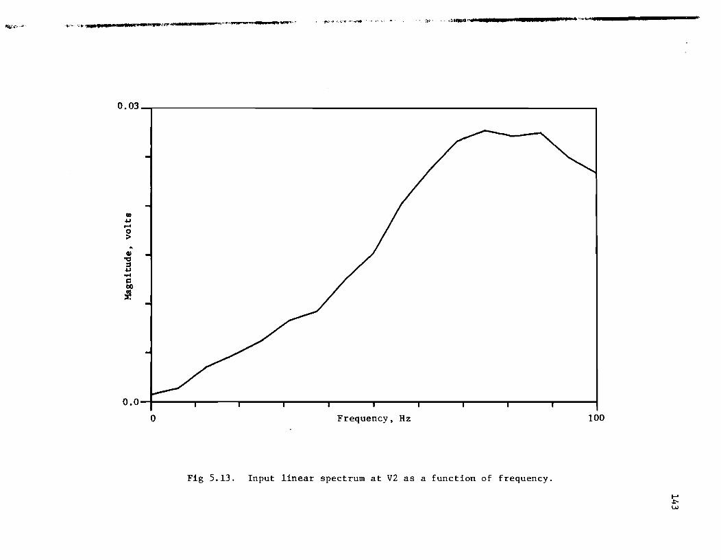
~'.",.'~ "\C-?' ·S'. 11 T 'ii9i'14",;/41'" b Il¥· .... ".... .... --- W4"""''''''' .,.,,.v_.!'f\..~--.. ,',.,~
it."'.. -:~....... .11 .· .. 41""_ .. _____________ _
0.03~------------------------------------------------------------------~
III
""' ..... o >
QI ." ::1
""' ..-4 c:: CO
~
O.OI----.--r----.----,.--r----.----.--r---~---J o Frequency, Hz 100
Fig 5.13. Input linear spectrum at V2 as a function of frequency.
I-' ~ w
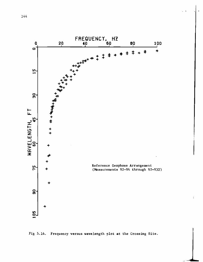
144
o o
In -o ('t)
o 0)
If) o -
+ +
+
.po
+
+
+
+
20 FREQUENCY, HZ
40 60 80 100
+
Reference Geophone Arrangement (Measurements V2-V4 through V2-V32)
Fig 5.14. Frequency versus wavelength plot at the Crossing Site.
.' .. "

I I
0.6
0.5
.... I ... I,j.j
l' 0.4 '-'
s:: 0 ~ ... «I :l s:: Q) ... 0.3 ... « I,j.j
0 Range ... s:: Q.I ~ U ~ 0.2 I,j.j I,j.j
Q.i 0 u
0.1 'I~d I I O.OL-------~--------~--------~------~--------~ o 20 40 60 80 100
Frequency, Hz
Fig 5.15. Variation of coefficient of attenuation with frequency at the Crossing Site.
145

146
Using the relationship a - 0.00195 f, values of a were calculated that
did not exhibit the scatter associated with the measured values. In
addition, values of the logarithmic decrement 0 and damping ratio D were
calculated using Eqs 2.9 and 2.10, respectively. Calculated values of a, 6,
and D are listed in Table 5.4. The damping ratio is expressed in percentage
and ranges from about 8 to 20 percent. The higher values associated with the
lower frequencies may have resulted from insufficient input energy at those
frequencies and/or from the fact that the longer wavelengths had not traveled
enough to obtain a representative reading, even for the farthest location of
geophones (measurement V2-V34).
The apparent large variation in damping as a function of frequency is
probably not due to actual differences in soil properties but, rather, is a
result of poorer data at the lower frequencies. To compare graphically the
attenuation of R-wave amplitude as a function of frequency, it is necessary
to establish a datum at which each frequency has the same initial magnitude.
The reference geophone V2 is the most convenient initial point since it
served as the input geophone for each measurement. For the sake of
comparison, the amplitudes at each frequency are assumed to equal unity at
V2, although the linear spectrum at V2 (Fig 5.13) indicates that the input
amplitude varied as a function of frequency.
ratios at other distances, then, each ratio must
spectrum amplitude at each particular frequency.
To "normalize" the amplitude
be divided by the input
These normalized amplitude
ratios (NAR) are listed in Table 5.3, and, in effect, represent the
amplitudes at the output geophones (V4, V6, V10, etc.) that would have been
measured if all frequencies had been given the same input energy.
In addition, a provision must be made to account for the fact that
higher frequencies will have undergone more wavelengths in a given distance

! t , i !
I
TABLE 5.4. RELATIONSHIP BETWEEN FREQUENCY AND DAMPING AT THE CROSSING SITE
Coefficient Logarithmic Damping Frequency Wavelength of Decrement Ratio
Attenuation f(Hz) ~(ft) a(ft-1) 0 D(i.)
10 64 0.020 1.25 19.5
12 42 0.023 0.98 15.4
14 34 0.027 0.93 14.6
16 30 0.031 0.94 14.8
20 24 0.039 0.94 14.8 25 18 0.049 0.88 13.9
30 14 0.059 0.82 12.9
40 9.5 0.078 0.74 11.7 50 7.1 0.098 0.69 10.9 60 5.1 0.117 0.60 9.5 80 3.3 0.156 0.51 8.1
100 2.6 0.195 0.51 8.1
147

148
than lower frequencies. Frequencies can be compared on an equal basis by
using the number of cycles the wavelength has undergone as opposed to the
actual travel distance. The number of cycles can easily be calculated from
Eq 4.7 if the wavelength for a given frequency is known. Table 5.3 contains
values for the number of cycles for each frequency at each geophone location.
These values are plotted versus NAR for selected frequencies in Fig 5.16.
The trend in the data indicates that all frequencies (from 10 to 100 Hz)
exhibit the same damping behavior.
This conclusion was also drawn from the data at the Walnut Creek site
which are shown in Fig 4.31. As was the case at Walnut Creek, it is
difficult to determine whether the high values for D are excessive because of
body wave energy present in the wave pulse at V2 or if the values are
realistic estimates of field damping caused by backscattering that is indeed
higher than damping measured in the laboratory. The former difficulty could
possibly be avoided by using a reference geophone at 8 to 10 ft, thus
allowing the body wave energy to dissipate prior to reaching the first
geophone.
SUMMARY
Results and conclusions based on tests performed at The Crossing are
quite similar to those found from soil testing at Walnut Creek.
Velocity profiles obtained from cross spectrum (surface) measurements
tend to exhibit some scatter. Much of this scatter can be reduced by
filtering out data for wavelengths which are inappropriate for the spacing of
geophones. Using criteria developed from the Walnut Creek site, data from
the Crossing site was filtered to produce a refined velocity profile.
~-~.~;-::-... ~.......- - ~ ~-,-, ... --------------~~~~~-
. I
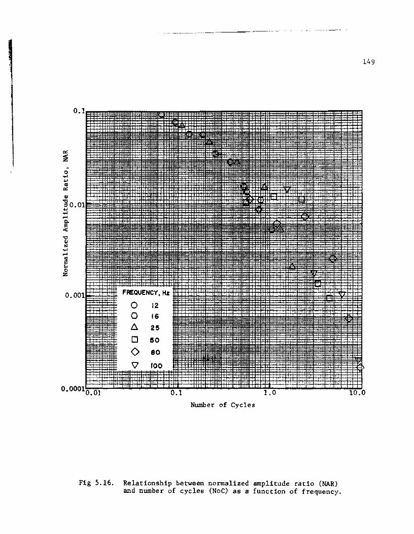
o.
~
;! A
0 ..... .j.I
III ~
~ "C ::I O • .j.I ..... ~
! "C ~ N ..... ~
~ ~ 0
Z
O.
o.
0 12
0 16
A 2S
D so 0 80
\l roo
Number of Cycles
Fig 5.16. Relationship between normalized amplitude ratio (NAR) and number of cycles (Noe) as a function of frequency.
149

150
The velocities obtained from cross spectrum measurements using an
equally spaced geophone arrangement were, on the average, higher than those
obtained from measurements made using a reference geophone arrangement. The
difference in velocities increased with increasing wavelength, suggesting
that the reference geophone was located too close to the source to sample
long wavelengths adequately. The velocity profile from measurements using
equally spaced geophones correlated well with crossho1e results when the
profile was plotted using a depth criterion of ~/3. In general, cross
spectrum velocities did not vary by more than 10 percent from crossho1e
velocities.
Attenuation properties at the site were evaluated by means of transfer
functions. For attenuation calculations, better data were obtained using the
reference geophone arrangement than were obtained using the equally spaced
geophone arrangement. The coefficient of attenuation was found to be
approximately a linear function of frequency and was estimated by
a - 0.00195 f. Values of logarithmic decrement and damping ratio were also
calculated, with values of damping ranging from about 8 to 20 percent. These
values are somewhat higher than those typically measured in laboratory tests,
perhaps due to excessive body wave energy present at the near geophone (but
not present at the far geophone). This problem could possibly be overcome by
locating the reference (near) geophone at a distance of 8 to 18 ft from the
source.
••

~---~-~-------~ -.---~-.-."
CHAPTER 6. PAVEMENT EVALUATION AT AUSTIN SITE
SITE DESCRIPTION
The Austin site is located about 2 miles (3.2 km) northeast of the
campus of The University of Texas at Austin, as shown in Fig 6.1. The
selected site is a flexible pavement section of IH 35 at Sta 670+00, which is
located near Capital plaza Shopping Center. All testing was conducted in the
extreme right-hand lane on the northbound portion of the highway_
The longitudinal section profile is shown in Fig 6.2. The profile is
based on borings which were made in conjunction with crossho1e testing. The
asphalt layer consists
approximately 2.5 in.
of a hot mix asphaltic concrete (HMAC) surface
(6.4 em) thick and an asphalt-stabilized base
approximately 4 in. (10.2 cm) thick. The unit weights and Poisson's ratios
of these materials were assumed to be 145 pcf and 0.35, respectively. The
flexible base of crushed limestone was compacted in three layers, each
approximately 5 In. (12.7 em) thick, with a unit weight of 140 pcf and a
Poisson's ratio of 0.40. The base course grades into a subbase of dense sand
with a layer thickness of about one foot (0.3 m).
black stiff clay grading into a tan silty clay.
Poisson's ratio of the subgrade were assumed to
respectively.
The natural subgrade is a
The unit weight and
be 115 pcf and 0.40,
12.5 to 13 ft (3.8 to Borings were terminated at a depth of
151

152
CAPITAL PLAZA
THE UNIVERSITY
OF TEX7
D
SITE·
Fig 6.1. Location of Austin (IH 35) Pavement site.
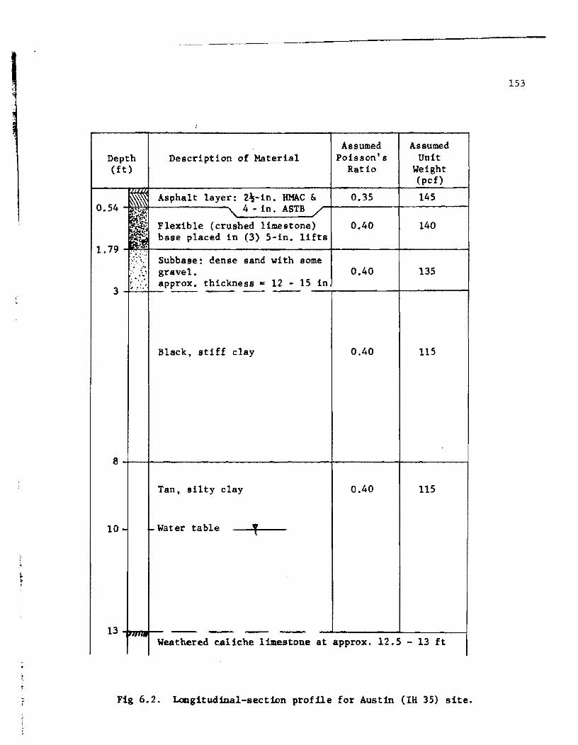
153
Assumed Assumed Depth Description of Material Poisson's Unit (tt) Ratio Weight
(pcf)
~ Asphalt layer: 2%-in. HMAC& 0.35 145 0.54
I 4 • in. ASrB
~~ Flexible (crushed limestone) 0.40 140 .... c.'. base placed in (3) 5-in. lifts .Ii"
1. 79 ,
.~;'::.;/ Subbase: dense sand with some
.,; .. ~ gravel. 0.40 135 : ... '"".!
; .... ~ approx. thickness = 12 - 15 in ;, ' .. :./ 3 -- -- -
Black, stiff clay 0.40 115
8~~--------------------------~------~--------~
Tan, silty clay 0.40 115
10 - I- Water table
13"" .. ----Weathered caliche limestone at approx. 12.5 - 13 ft
Fig 6.2. Longitudinal-section profile for Austin (Ia 35) site.

154
4.0 m), the depth at which rock was encountered. The water table was located
at a depth of about 10 ft (3 m).
Due to the heavy traffic at the site, a small amount of undesirable
background noise was present during testing. In addition, power to operate
electrical equipment had to be provided by a portable generator, which also
contributed some background noise at the site.
EXPERIMENTAL PROCEDURE
Initially, only surface measurements were performed at the Austin site.
These tests were conducted on May 19-20, 1980. No borings were made at this
time, so as to keep within the .restraint of nondestructive testing.
Subsequently, crossho1e tests (and borings) were performed on September 15,
1980, to verify the section profile as well as check the accuracy of the
velocities obtained from surface measurements. The equipment and general
procedure are discussed in the following sections.
Equipment
Two different sources were used to propagate waves through the pavement
system. Each source generated an impulsive load on the surface of the
pavement.
digital
Therefore, all signals
analysis of the signals
using a rectangular window.
were transient events. Truncation for
in the frequency domain was accomplished
The primary source was a Falling Weight Def1ectometer (FWD), similar to
the Phoenix Falling Weight Def1ectometer manufactured in Denmark (Ref 3).
This device was mounted on a two-wheel trailer that could be towed on the
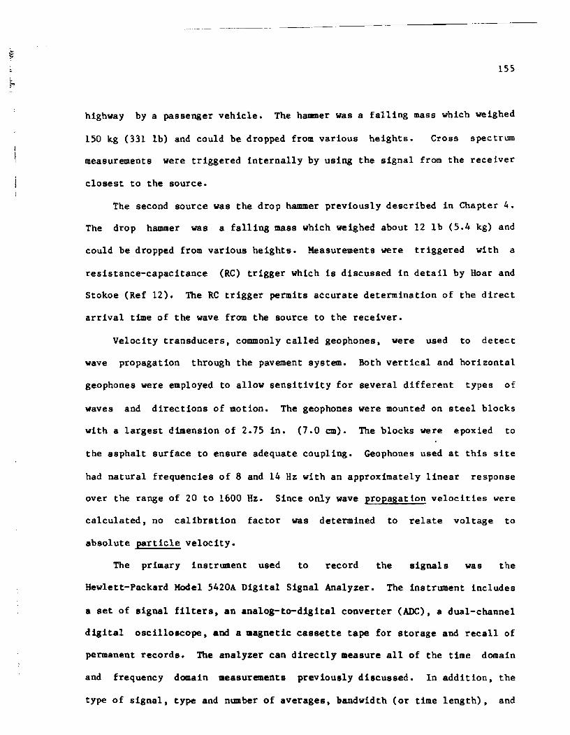
------------------~---------
155
highway by a passenger vehicle. The hammer was a falling mass which weighed
150 kg (331 lb) and could be dropped from various heights. Cross spec truro
measurements were triggered internally by using the signal from the receiver
closest to the source.
The second source was the drop hammer previously described in Chapter 4.
The drop hammer was a falling mass which weighed about 12 lb (5.4 kg) and
could be dropped from various heights. Measurements were triggered with a
resistance-capacitance (RC) trigger which is discussed in detail by Hoar and
Stokoe (Ref 12). The RC trigger permits accurate determination of the direct
arrival time of the wave from the source to the receiver.
Velocity transducers, commonly called geophones, were used to detect
wave propagation through the pavement system. Both vertical and horizontal
geophones were employed to allow sensitivity for several different types of
waves and directions of motion. The geophones were mounted on steel blocks
with a largest dimension of 2.75 in. (7.0 em). The blocks were epoxied to
the asphalt surface to ensure adequate coupling. Geophones used at this site
had natural frequencies of 8 and 14 Hz with an approximately linear response
over the range of 20 to 1600 Hz. Since only wave propagation velocities were
calculated, no calibration factor was determined to relate voltage to
absolute particle velocity.
The primary instrument used to record the signals was the
Hewlett-Packard Model 5420A Digital Signal Analyzer. The instrument includes
a set of signal filters, an analog-to-digital converter (ADC), a dual-channel
digital oscilloscope, and a magnetic cassette tape for storage and recall of
permanent records. The analyzer can directly aeasure all of the time domain
and frequency domain measurements previously discussed. In addition, the
type of signal, type and number of averages, bandwidth (or time length), and
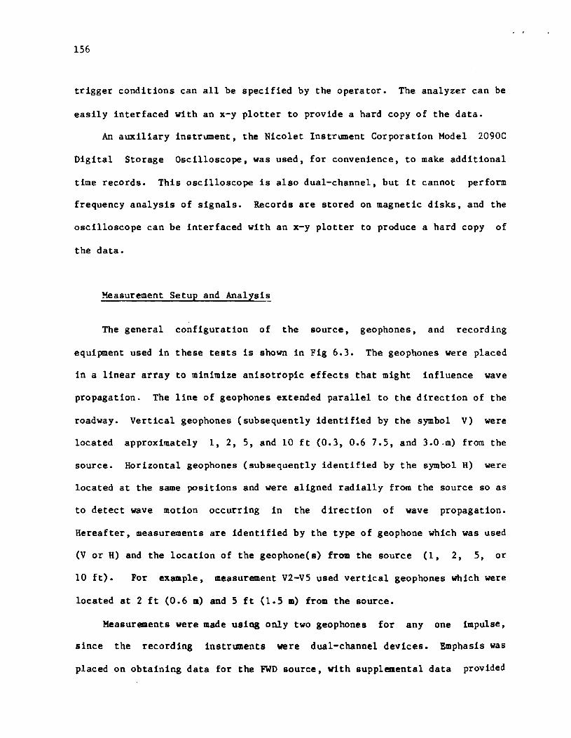
156
trigger conditions can all be specified by the operator. The analyzer can be
easily interfaced with an x-y plotter to provide a hard copy of the data.
An auxiliary instrument, the Nicolet Instrument Corporation Model 2090C
Digital Storage Oscilloscope, was used, for convenience, to make additional
time records. This oscilloscope is also dual-channel, but it cannot perform
frequency analysis of signals. Records are stored on magnetic disks, and the
oscilloscope can be interfaced with an x-y plotter to produce a hard copy of
the data.
Measurement Setup and Analysis
The general configuration of the source, geophones, and recording
equipment used in these tests is shown in Fig 6.3. The geophones were placed
in a linear array to minimize anisotropic effects that might influence wave
propagation. The line of geophones extended parallel to the direction of the
roadway. Vertical geophones (subsequently identified by the symbol V) were
located approximately 1, 2, 5, and 10 ft (0.3, 0.6 7.5, and 3.0.m) from the
source. Horizontal geophones (subsequently identified by the symbol H) were
located at the same positions and were aligned radially from the source so as
to detect wave motion occurring in the direction of wave propagation.
Hereafter, measurements are identified by the type of geophone which was used
(V or H) and the location of the geophone(s) from the source (1, 2, 5, or
10 ft). For example, measurement V2-VS used vertical geophones which were
located at 2 ft (0.6 m) and 5 ft (1.5 m) from the source.
Measurements were made using only two geophones for anyone impulse,
since the recording instruments were dual-channel devices. Emphasis was
placed on obtaining data for the FWD source, with supplemental data provided

5f
-------- ~... -----~-------... -- ---
Spectral Analyzer
Oscilloscope
Control Panel
ADC
Ch1 Ch2 ig
Vertical
Fig 6.3. Schematic diagram of experimental setup.
157

158
by the drop hammer source. Both time domain and frequency domain
measurements were recorded, although the thrust of the data acquisition was
toward spectral analysis. - Table 6.1 contains a listing of the various
pairings of geophones, the exact distances between the geophones, the source,
and the bandwidth for each measurement. Time domain measurements included
time record averaging, autocorrelation, and cross-correlation. Frequency
domain measurements included the linear spectrum, autospectrum, cross
spectrum, transfer function, and coherence function.
The analysis of the cross spectrum data followed the general procedure
outlined in Appendix A. Various parameters were studied to determine their
influence on the cross spectrum measurements. Records with one average and
five averages were used to compare the advantages of averaging. Comparative
measurements were made for responses of both vertical and horizontal
geophones. The effectiveness of each source was also investigated. Results
of these comparisons are presented in the following section.
RESULTS FROM SURFACE MEASUREMENTS
Comparisons for both time and frequency domain measurements indicate
that there are no significant differences between one-average records and
five-average records. This is probably a result of the high reproducibility
of the impulse. However, one-average records occasionally exhibited apparent
anomalies. To avoid anomalies, all analyses were performed using
five-average records.

TABLE 6.1. SUt1MARY OF MEASUREMF.NTS AT THE AUSTIN (IH 35) SITE
Record No. Channel Plat.nce Source Number BandwIdth Input between of of
11 12 Geophonea Ave rage a Spectru. (ft) (Hz)
22 V5 VlO 5.02 Falling Weight Deflectometer 1 400
29 VI V2 1.00 II " " ,5 200
51 & 55 V2 V5 3.08 II It " 165 100
101 6 106 V2 V5 3.08 .. .. .. 165 1600
59" 64 H2 BS 1.08 Of .. .. 1 " 5 100
69" 74 H2 HI0 8.10 .. " .. 1 & 5 100
79 & 84 V2 VlO 8.10 .. " .. 1 & S 100
91 6 96 V2 VIO 8.10 .. .. " 1 & 5 1600
114 H2 H5 3.08 Pl'Op Hanner 5 1600
119 V2 V5 3.08 .. " S 1600
Co..,uUl' Data Fne
Identification
SHCPJ
SHCPI
SHCP2
SHep2
SHCP5
SHCP6
SHCP4
-SHepS
SRCP7
I-' Vl \0

160
Comparison of Horizontal and Vertical Geophones
In general, the coherence functions were similar for measurements with
the same geophone locations, regardless of whether the geophones were
oriented horizontally or vertically. The range of frequencies measured by
the cross spectrum was also similar regardless of geophone orientation.
Based on the magnitudes of the cross spectrums for measurements with the drop
hammer as the source, the levels of excitation energy in the horizontal and
vertical directions are of the same order of magnitude. In contrast, for
measurements with the FWD as the source, the magnitudes of the cross
spectrums for measurements using vertical geophones were approximately 100
times greater than the magnitudes for measurements using horizontal
geophones. This result is not unexpected, since the FWD is designed to input
a large force in the vertical direction to create a deflection basin.
Although the range of frequency response was similar for both
orientations of geophones, the velocities obtained from measurements using
horizontal geophones were significantly higher than those obtained from
measurements using vertical geophones. This trend was true for measurements
made with both the FWD and the drop hammer. Since the horizontal geophones
are much more sensitive to P-wave motion than the vertical geophones, it is
quite likely that spectrums for measurements using horizontal geophones
contain some higher-velocity P-wave energy which leads to an overall higher
velocity for the (apparent) R-wave.
Such a hypothesis can be checked, at least in part, by comparing time
records of wave pulses obtained from horizontal and vertical geophones.
Figure 6.4a shows time records obtained with the Nicolet oscilloscope for
horizontal geophones H2 and HlO (FWD source). For the interval travel time
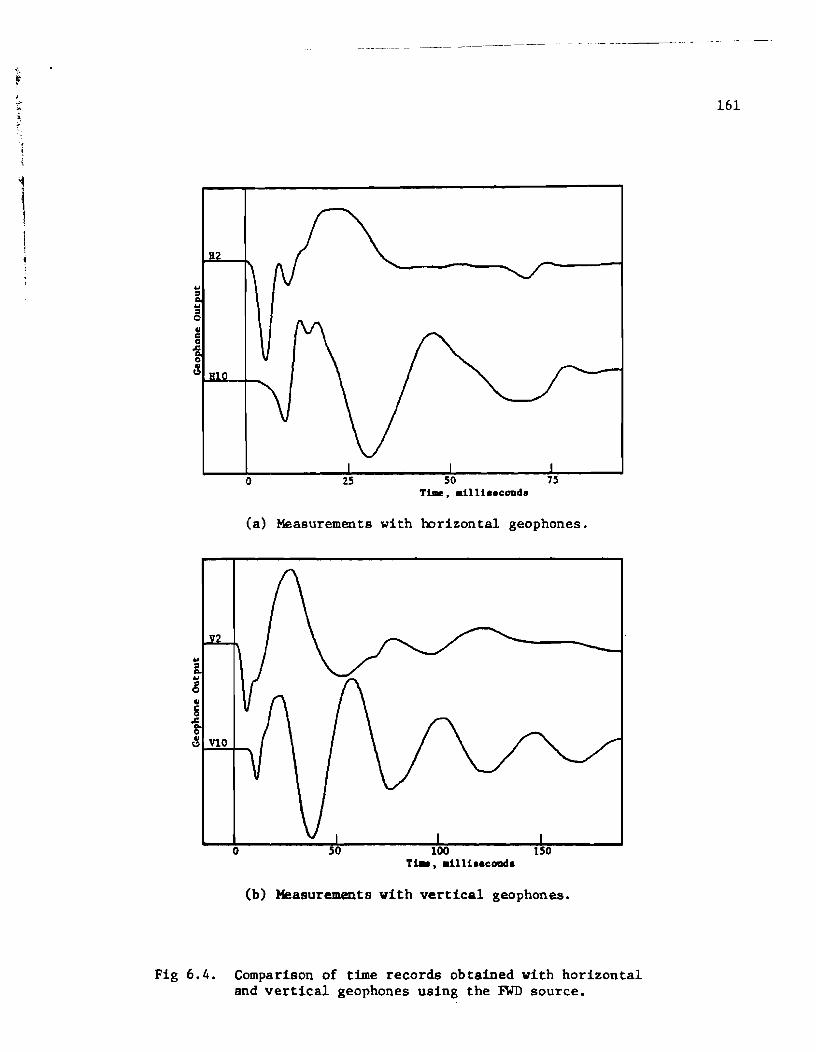
-- ------------
o 2S 50 75 Time, .illl •• caad.
(a) Measurements with horizontal geophones.
Tt.e, al11l •• coada
(b) Measurements with vertical geophones.
Fig 6.4. Comparison of time records obtained with horizontal and vertical geophones using the FWD source.
161
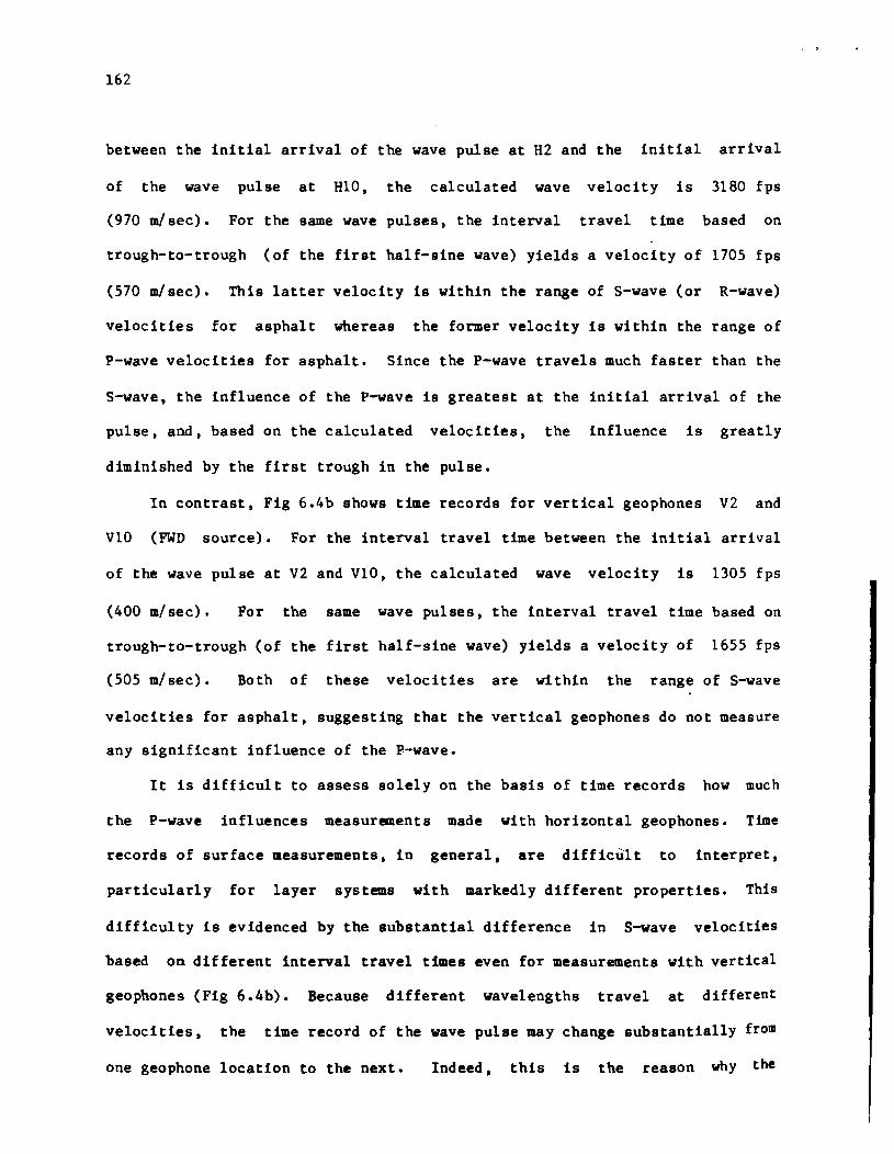
162
between the initial arrival of the wave pulse at H2 and the initial arrival
of the wave pulse at H10, the calculated wave velocity is 3180 fps
(970 m/sec). For the same wave pulses, the interval travel time based on
trough-to-trough (of the first half-sine wave) yields a velocity of 1705 fps
(570 m!sec). This latter velocity is within the range of S-wave (or R-wave)
velocities for asphalt whereas the former velocity is within the range of
P-wave velocities for asphalt. Since the P-wave travels much faster than the
S-wave, the influence of the P-wave is greatest at the initial arrival of the
pulse, and, based on the calculated velocities, the influence is greatly
diminished by the first trough in the pulse.
In contrast, Fig 6.4b shows time records for vertical geophones V2 and
V10 (FWD source). For the interval travel time between the initial arrival
of the wave pulse at V2 and V10, the calculated wave velocity is 1305 fps
(400 m/sec). For the same wave pulses, the interval travel time based on
trough-to-trough (of the first half-sine wave) yields a velocity of 1655 fps
(505 m/sec). Both of these velocities are within the range of S-wave
velocities for asphalt, suggesting that the vertical geophones do not measure
any significant influence of the P-wave.
It is difficult to assess solely on the basis of time records how much
the P-wave influences measurements made with horizontal geophones. Time
records of surface measurements, in general, are difficult to interpret,
particularly for layer systems with markedly different properties. This
difficulty is evidenced by the substantial difference in S-wave velocities
based on different interval travel t~es even for measurements with vertical
geophones (Fig 6.4b). Because different wavelengths travel at different
velocities, the time record of the wave pulse may change substantially from
one geophone location to the next. Indeed, this is the reason why the

-~~------~ --------------
163
spectral analyzer is used to isolate the propagation of individual
frequencies within the measurement bandwidth.
The phase plots of the cross spectrums for measurements V2-VI0 and
H2-H10 are shown in Fig 6.5. In general, the phase for a particular
frequency is less for measurement H2-RIO than the phase at the same frequency
for measurement V2-VIO. A lesser phase translates into a lesser travel time
and, hence, a greater velocity for the wavelength at the particular
frequency. For example, at 30 Hz, the phase for measurement H2-HlO is 111.01
degrees, which yields a velocity of 788 fps (240 m/sec), while the phase for
measurement V2-VIO 1s 149.44 degrees, which yields a velocity of 586 fps
(179 m/sec) for a difference in velocities of 34 percent.
The most important and conclusive comparison involves the velocity
profile obtained with measurements using vertical geophones versus the
profile obtained with measurements using
compares the velocity profiles (using
horizontal geophones. Figure 6.6
~/3 as the "effective" depth) for
measurements V2-V5 and H2-H5 using the drop hammer source. In each layer,
the velocities from H2-H5 are distinctly greater than velocities from V2-V5.
The velocity profile from V2-VS correlates extremely well with shear wave
velocities from crosshole tests verifying that measurements with vertical
geophones are more reliable than those
result, nearly all of the analysis
testing at other sites) included only
geophones.
with horizontal geophones. As a
for the Austin site (and subsequent
measurements made with vertical
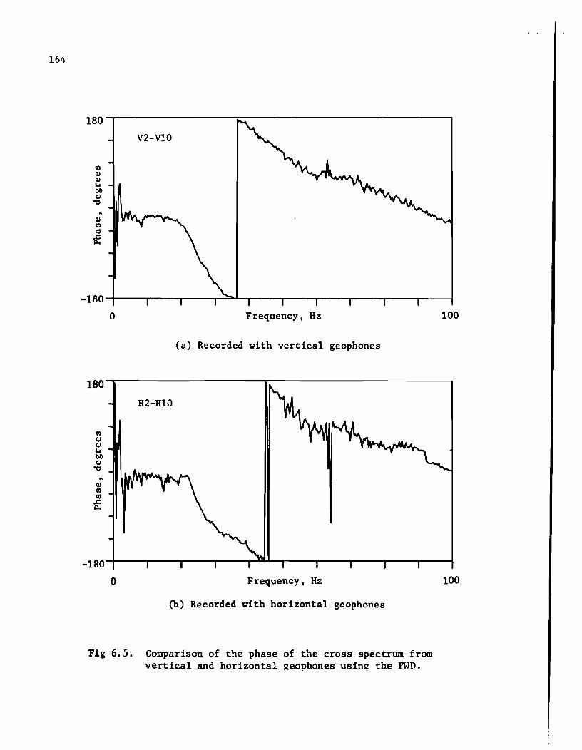
164
180
QJ CD co f
V2-VlO
-180-+----T---~----,-~~----,---~~--_r----r_--_r--~
180
CD QJ QJ ... CIO QJ
"0
QJ CD co f
-180
o
o
Frequency, Hz
(a) Recorded with vertical geophones
H2-H10
Frequency, Hz
(b) Recorded with horizontal geophones
Fig 6.5. Comparison of the phase of the cross spectrum from vertical and horizontal ~eophones usine the FWD.
100
100

o o
N
•
...... LL..CD
.. :t: ...... Q.. L&J CeD
o -
N -
• -
VELOC I TY, .0 80
As halt
Base (!)
C!)
19 C!) Subbase
f-e C!)
Subgrade r C!)
19m C!) 19 C!)
19 C!) C!) C!)
19
19
e 19
C!)
19
19
o Vertical Geophones o Horizontal Geophones
C!)
FPS -10 120 160 200
Fig 6.6. Comparison of velocity profiles obtained ~ith vertical and horizontal geophones using the Drop Hammer source.
165

166
Analysis of the Falling Weight Def1ectometer
The complete time history of the falling weight is shown in Fig 6.7a.
The signal was recorded from a geophone attached to the base of the FWD. The
signal was triggered (t - 0) with the initial downward hit of the weight. A
pre-trigger delay was used to capture the "negative time" part of the signal.
(The use of a pre-trigger delay to capture the signal is discussed in
Appendix A). The small upward displacement at approximately t = -0.25 sec is
due to the slight rebound of the base plate when the weight is released to
undergo free fall. Multiple impacts occur for about eight or nine rebounds
of the weight. These additional impacts do not interfere with the initial
pavement response, because all data is collected from each impulse before the
next impulse occurs. The time interval for a wave travelling from 2 to 10 ft
(0.6 to 3.0 m) is on the order of 10 milliseconds, whereas the interval time
between the first and second impacts of the weight is approximately
450 milliseconds.
The Fourier transform of the time signal, the linear spectrum, is shown
in Fig 6.7b. The major frequency component excited by the falling weight is
approximately 21 Hz.
the first trough of
This corresponds quite closely to the pulse created by
the signal
approximately 25 mill isecond s,
in the time domain. This pulse width is
yielding a predominant period
T - 50 milliseconds, or a predominant frequency of 20 Hz. The level of
excitation greatly decreases with increasing frequencies.
The response of the pavement using the FWD for measurement V2-V5 is
shown in Fig 6.S. Both the transfer function and the cross spectrum indicate
that most of the response centers about the predominant frequency of
~ -'1""-- -F4C , ..

4·o-r-------------------~-------A~d~d~1~·t-i~o-n-a~I~1ID~·-p-a-c-t-s--f~r-o-m---------,
Release ,. weight bouncing::.,.._-::o.., of we?
First impact of weight ~
·4.
-0.5 Time, seconds 2.0
(a) Time-history of motion
0.15-r--------,-----------------------------------.
CD .j,.J .... o :> .... .... .... .... E
.j,.J
:::I Q.
.j,.J
=' o 41 £: o .c: 0.. o 41 c
-O.15~--~r_--~--_r--~r_--,_--~----r_--,_--~--~
o Frequency, Hz
(b) Linear .pectrum of motion
Fig 6.7. Impulsive loading created by the Falling Yeight Deflectometer.
100
167

168
0.8
O~----r----r----r---~~~~--~--~------------~
3.0
QI C o
,.c:: no QI t!)
0.0
o
-
-
-
-
-
o
Frequency, Hz
(a) Transfer Function
J,. u~ \ IJ\MA " I I I I I I I I I
Frequency, Hz
(b) Cross Spectrum
Fig 6.8. Pavement Response for measurement V2-VS using the FWD source.
100
100

169
excitation of the source itself (21 Hz). Similar responses were obtained for
other combinations of receivers.
The velocity profile for measurements with the FWD was determined from
phase information of the cross spectrum obtained from plots such as the one
in Fig 6.5a. A typical set of calculations is shown in Table 6.2. Depths
given in the table were calculated using the one-third wavelength criterion.
The resulting profile is shown in Fig 6.9.
There is some scatter in the velocities for measurement VI-V2. This
scatter may be due to the fact that the geophones are located too close to
the source to sample properly the wavelengths which travel primarily in the
base and subgrade. As a result, the phase difference is small between the
two geophones, and the measurement is more sensitive to the experimental
limitations of the spectral analyzer (see Chapter 4). Also, the longer
wavelengths will not have travelled far enough to be influenced adequately by
the material properties at a depth which the wave(s) supposedly sampled. The
velocities will then be overweighted by the material properties near the
surface, particularly by the higher-velocity asphalt surface layer.
Based on Fig 6.9, R-wave velocities in the base and subgrade were
estimated to be BOO fps (270 m/sec) and 580 fps (175 m/sec), respectively.
In the zone where the base course grades into the sandy subbase, the velocity
contrast is not as distinct, but it appears that a reasonable estimate of the
i-wave velocity in the subbase is about 700 fps (215 m/see). Velocities
could not be determined (with the FWD as the source) for the upper 15 in.
(38 em) of the profile. For typical velocities of pavement materials, the
FWD cannot excite frequencies high enough to generate the short wavelengths
needed to sample the upper layers.
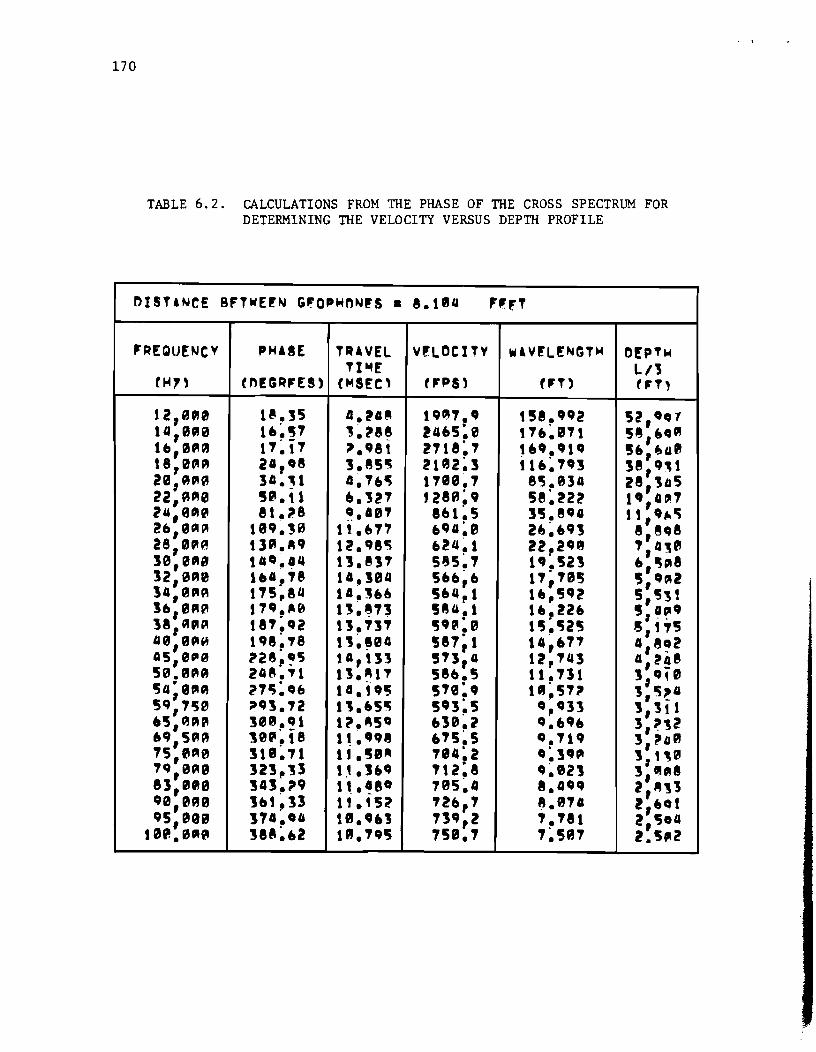
170
TABLE 6.2. CALCULATIONS FROM THE PHASE OF THE CROSS SPECTRUM FOR DETERMINING THE VELOCITY VERSUS DEPTH PROFILE
DIST&NeE BFTWE~N G~O'~nN~S • 8.1~4 F'FT
FREQUENCV P~&8E T"&VEL V'LOCITY w&V~L!NGT~ O!PT~ Tl"£ L 1'5
004" (nEGItFES) (MSEC' tFPS) t'T) tF"
lZ,0C11~ 1~.35 4.P'~ lC,~'.C, t51.C,C,2 52,"7 14,9A" I"~~' '~~8~ 24"5:0 t'''~B'l 5~,"'C11 le,,~CII" l'~i'7 it.C,8t 2'18~'7 t"C,~C,I' 5",~"1I t8,e",,,, il.'S 3.85'; 21l!12~3 tl".'7C,3 31,C"t ze,"''''~ 34:'1 4.'6~ 1,ee., 81§~B34 Z8,'545 2Z,A~0 5P.tl ".'52'7 '280~C, 58:2Z~ 1',4'" 24,""'0 8t.i'8 ~.O'U 861.5 315.SC,1 tt,' __ 1Ii
2e"e~~ IBC,.39 It.''''7 6c,a~0 2fJ~"q3 8,e,s 28,0"'''' tl"'.AQ 12.C,811\ 624~1 ZZ.2C,1/J '7,0,0 30,""''' 14'.44 13.1]'7 51}5~' t'~5il ",~"'8 ]2,0~0 1e,4.;e 10.le4 566~6 1'7~'7QJ5 ~,''''Z 30,11.1"'''' !'5~84 14.J"~ 5"4,1 1",15C,2 5,1S3\ 1e",,1'1~ t'C,.~0 13~~" 584.1 1",22" 5,~~C, 38.APlA t8'7~'2 13.'73' l5c,rII:e II5.I§Z5 ~,1'15 4e;e"'i4 IC,8:,8 13~~"0 587;1 t4~"''7 4,8!t Z A5,0"'9 ~28~~5 t A,t33 5'73,4 12,'43 4,~!1 59.""'''' 24~."1 11.~I' 58b.5 11.'31 1,'10 154;e",,, 2'-;:'6 lG.1C,15 5'7e:c, UJ~5'7l' 1,~~4 5C,,'50 ;:tC,l.'Z 1'."S'i 5C,3~5 '.'33 1,111 '15,~PlPI 3I!JC!I~!1 ttt.~5' 630~l '~6C,,, 3,~'2 'Q,5P1" 10r11.t8 It~'C,8 ''75~5 0.'71C, 3,l'tle '5,"1110 lle~"1 tt.5"~ '7e4~2 0:3'''' 1,110 '7c',""''' 323,13 t.t .160 ,t2;8 '~1!J21 3,""'8 83,1!J1I" 14].~q I\.~eo '05~4 8.4C,C, 2,A,3 C,0,0l!1" 16t~]1 11 .' 5~ '26,' A.CIJ" 2,,,ot c,5,eel!l 3'4~04 te.'.1 '3C,,2 '.'81 2,1504
tQJP..I!J"'tlII ]88~"Z IIIJ.'C,I§ '5".' '~5"'7 2.5(11Z

o o
Asphalt
- Base
Subbase
Sub grade
VELOCITY. 30 60
C!)
FPS -10 90
C!)
cf C!)
I!J I!J C!)
I!J C!)
I!J I!J
J!C!) I!J A
e9. c!)c!) ~ ~AA
I!J
C!) A I!J I!J
I!J A I!J
C!)
AI!J
C!)
d" A I!J A
AC!) C!)
AC!)
I!J mC!)
• C!)
II
120
Measurement
o Vl-V2 o V2-V5 l:::. V2-VIO
Fig 6.9. Velocity profile obtained from measurements using the FWD source.
171
150

172
Previously, it was shown that the level of excitation of the FWD
decreased with increasing frequency (Figs 6.7
illustrated even more clearly by comparison
and
of
6.8). This trend is
the autospectrum over
different bandwidths shown in Fig 6.10. Nearly all of the energy of
excitation is contained within 100 Hz and essentially no frequencies are
excited above 250 Hz. Figure 6.11 shows the cross spectrum and coherence for
measurement V2-V5 over a 1600-Hz bandwidth. Above 250 Hz, the phase of the
cross spectrum becomes erratic. Similarly, the coherence displays
irregularities above 250 Hz. These plots indicate that the FWD does not
sufficiently excite the necessary frequencies to test the entire pavement
system.
Analysis of the Drop Hammer
Measurements with the drop hammer source were made using one pair of
horizontal geophones, H2-H5, and one pair of vertical geophones, V2-V5.
Figure 6.12 shows the autospectrum of the signal at geopho~e V2. The
magnitude indicates that all of the frequencies up to about 1600 Hz are
sufficiently excited to determine a valid pavement response for all layers of
the system. The phase of cross spectrum and the coherence function for
measurement V2-V5 are shown in Fig 6.13. Although the cross spectrum looks
fine up to 1600 Hz, the coherence function drops off sharply at about 1300 to
1400 Hz, suggesting that data above 1300 Hz should be used with caution.
The velocity versus depth profile is shown in Fig 6.14. This profile is
based on the phase information from measurement V2-V5 (Fig 6.13a) and is
plotted using La!3 as the depth criterion.
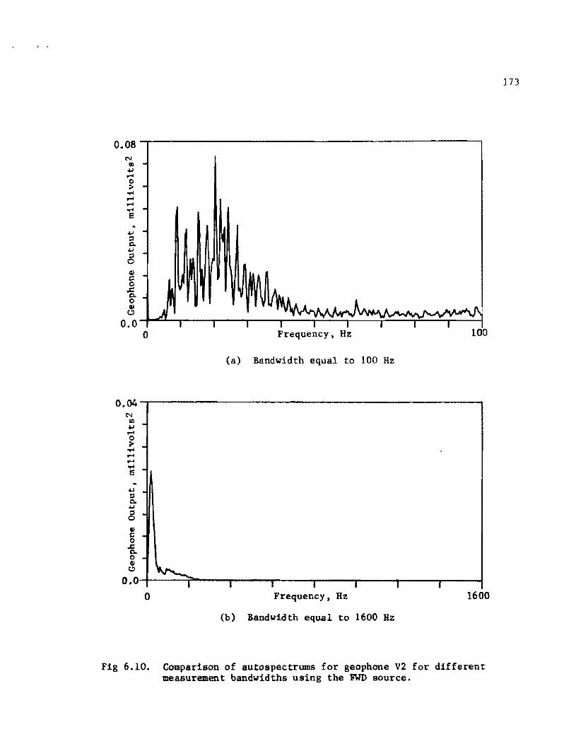
0.08 N
II)
+J .... 0 ;>
..-I .... ....
..-I e
+J ::I c. +J :;l 0 <1/ t::: 0
i. 0 <1/
c.!)
0.0 0 Frequency, Hz 100
(a) Bandwidth equal to 100 Hz
0.04-r----------------------------------------------
~ -C. +J
5 -<II g •
,s;; c. o •
~ ~ o.O-r----~I-----~I--~I-----r-I-.-.~I-----r-I----I----~
o Frequency, Hz 1600
(b) Bandwidth equal to 1600 Hz
Fig 6.10. Comparison of autospectrums for geophone V2 for different measurement bandwidths using the FWD source.
173

174
180~--~--------------------------------------------'
Qj CD CIf
of
-180~----~----~----~----~~----~----~----~--~
Qj u E:: Qj ... Qj
.c o u
o Frequency, Hz 1600
(a) Phase of cross spectrum
O~----~~----~-----r----~------~----~-----'----~
o Frequency, Hz
(b) Coherence function
Fig 6.11. Cross spectrum phase and coherence function for measurement V2-VS using the FWD source.
1600

O.002~----------------------------------------------
o.o~----~----~----~----~----__ ----__ --__ ~--~ o Frequency, Hz
Fig 6.12. Magnitude of the autospectrumfor geophone V2 using the Drop Hammer source.
175

176
180-r--~--------------------------~----------~
(a) Phase of the cross spectrum
1.0-r~--r-~~--------------------~~------~
+ 60-Hz noise
o Frequency, Hz
(b) Coherence function
Fig 6.13. Cross spectrum phase and coherence function for measurement V2-V5 using the Drop Hammer source.
1600

o As halt
Base
N Subbase
Subgrade .. a-u...CD
• :J: a-Q.. I.LJ OCD
.N -.. -
VELCJC I TY. 30 60
ID
-t-ID
efJlD IDID ID
ID
ID
ID
ID
ID
FPS -10 90 120
--
ISO
--
Fig 6.14. Velocity profile obtained using the Drop Hammer source.
177

178
The layering in the velocity profile (based on velocity contrasts)
correlates well with the actual profile when the cross spectrum velocities
are plotted at a depth of ~/3. The subbase can be readily identified as a
separate layer. The subgrade shows an increase in velocity with depth which
probably is due to the influence of the underlying, higher-velocity rock.
Based on the profile in Fig 6.14, R-wave velocities were estimated as 1400,
860, 690, and 560 fps (425, 260, 210, and 170 m/sec) for the surface layer,
base, subbase, and subgrade, respectively.
Comparison of the FWD and the Drop Hammer
The usefulness of an impact hammer for measuring wave velocities depends
on how well the hammer excites the frequencies required to analyze the
pavement system. Figure 6.15 contains the Fourier transforms, or linear
spectrums, of the wave pulse generated by the FWD and the drop hammer
sources. The dashed lines in part (a) are the limits of the plot in part
(b). The FWD focuses its excitation energy about 20 to 25 Hz, while the drop
hammer does a significantly better job of exciting frequencies over the
entire 1600-Hz bandwidth. Similar trends were shown in the autospectrums for
both vertical and horizontal receivers at various distances from the source.
Figure 6.16 compares the magnitude of the cross spectrums for
measurement V2-V5 for the FWD and the drop hammer. Based on areas under the
plots in Fig 6.16, the total energy in the cross spectrum of the FWD is
roughly 35 times the energy in the cross spectrum of the drop hammer.
However, this is not a critical factor, since total energy is only an
indirect index of the stress level induced by the impact. More important is
the relative distribution of the energy. As expected from previous

, 20-r----------------------------------------------~ lI)
""' .... o _ l> .... .... .... .... e
""' 6. -
g -~-------------~- -- .
g -- --------- ----------a o <U t.!>
-10~-------~1------~1-------~1r---------~1-------~1------~1~------r-1---~
o Frequency, Hz 1600
(a) Falling Weight Deflectometer
1.5 lI)
""' .... 0 -l> .... .... .... .... -e
! -~ V :::s 0
~ -s:: 0 .c 0.. o -~
Cl
-1.5 I I I I I I I 0 Frequency, Hz 1600
(b) Drop hammer source
Fig 6.15. Comparison of the linear spectrums for different sources.
179

180
400-.----------------------------------------------.
\0 I o
-.-4 -
O-+~--_.Ir-----TI------Ir-----~I------r-I----'I------~I----~
o Frequency, Hz 1600
(a) Falling Weight Deflectometer
0.4
\0 I 0 .-4
401 ::I ~ 0. 40IN ::I II)
0401 .-4
III 0 c:: ~ 0 .c ~
0.111 0'0 III ::I ~401 ~
c:: ao ~
0 0 Frequency, Hz 1600
(b) Drop hammer source
Fig 6.16. Comparison of the magnitudes of the cross spectrums for measurement V2-V5 using different sources.

" ..... ~ ...... ~~--...... -~- .--.. -"~.---------
181
examination of the autospectrum, the energy of excitation is distributed
better by the drop hammer. OVer 98 percent of the energy in the FWD spectrum
is contained within the first 100 Hz of the band, whereas only 11 percent of
the energy in the drop hammer spectrum is contained in the first 100 Hz of
the band.
Another comparison involves the phase of the cross spectrum.
Figure 6.17a indicates that the FWD does not provide discernible information
above 250 Hz, while Fig 6.17b shows that the drop hammer provides unambiguous
data over the entire 1600-Hz bandwidth. As noted previously, the FWD cannot
adequately sample the surface layer. Although the FWD is a good impulse
source for deflection measurements due to its high stress levels, the drop
hammer is better suited for determination of wave velocities in the surface
layers •
The R-wave velocities obtained from the FWD and the drop hammer sources
are listed in Table 6.3. Despite the large difference in the input energy,
the velocities obtained from measurements using the two sources are virtually
the same. This suggests that a large, heavy source is not necessary for
determining wave velocities or moduli. In addition, over the range of
stresses induced by the drop hammer up to those induced by the FWD, the
moduli of the materials are not stress (or strain) sensitive. Average values
of the R-wave velocities were determined from which S-wave velocities were
calculated. The shear wave velocities in Table 6.3 are based on cross
spectrum (surface) .easureaents and can be compared directly with the shear
wave velocities from crosshole tests presented in the next section.

182
180-r--.-----------------------------------------~
-180~----,_----~----r_--~r_--~----~----~----~
(a) Falling Weight Deflectometer.
180-r--~----------------------------~----------~
o Frequency, Hz 1600
(b) Drop hammer source.
Fig 6.17. Comparison of the phase of the cross spectrums for measurement V2-V5 using different sources.

TABLE 6.3. SUMMARY OF R-WAVE VELOCITIES DETERMINED FROM CROSS SPECTRID1 MEASUREMENTS AT AUSTIN (IH 35) SITE
Material Approximate Unit Poisson's R-Wave Velocity (fps) Thickness Weight Ratio FWD Drop Average
(in. ) (pcf) Hammer
Asphalt 6.5 145 0.35 - 1400 1400
Base 15 140 0.40 880 860 870
Subbase 12 to 15 135 0.40 700 690 695
Subgrade 120 115 0.40 580 560 570
S-Wave Velocity
(fps)
1500
925
740
605
I
.·,ii ....... '"".;'~
..... 00 w

184
RESULTS FROM CROSSROLE TESTING
Crosshole testing was conducted at the Austin site approximately four
months after the surface measurements were made. During the interim period,
the right lane of northbound IR 35 remained closed to traffic. Thus, both
sets of measurements were performed on the section as constructed. The
following paragraphs briefly describe aspects of crosshole testing particular
to the Austin site. A more general discussion of the crosshole seismic
method is presented by Stokoe and Hoar (Ref 12).
Description of Test Procedure
A diagram of the crosshole test setup is shown in Fig 6.18. The
boreholes were advanced in stages so that both the source(s) and geophones
could be situated at the bottom of the holes for selected depths, as shown in
Fig 6.18. Two holes, approximately 8 ft (2.4 m) apart, were drilled to a
depth of about 12.5 to 13 ft (3.8 to 4.0 m). One of these holes served as
the source hole for measurements made in the subbase and subgrade. The other
hole served as the receiver (geophone) hole. An additional hole, located
4 ft (1.2 m) from the receiver hole, was drilled to a depth of approximately
1.5 ft (0.5 m) and served as a source hole for measurements in the asphalt
and base course. This additional source hole was used to avoid refracted
waves from the higher-velocity surface layer.
Two sources were used to generate body waves (P- and S-waves) in the
various layers. Within 1.5 ft (0.5 m) of the surface, the drop hammer was
used. The drop hammer was placed so that its base plate rested on the bottom
of the hole. Measurements were triggered with an RC trigger. Below 1.5 ft
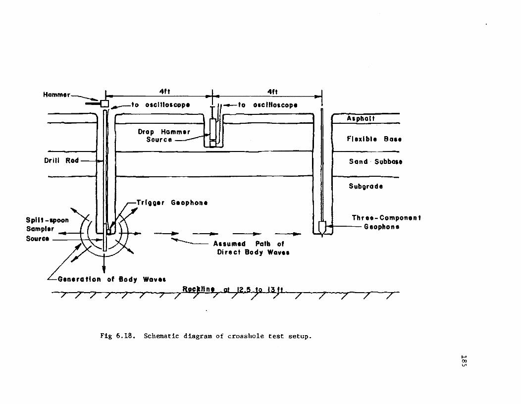
Hamm.r :::::.c5 4ft f 4ft I ~... .... ... _to olclllolCODI ~ '1-'0 olclllolCODI
1
o
SplttSomp. Source
rill Rod
:oon?{ \ -
- .
Drop Hommer Source ----- 1-10-
RT"U.' Geophon.
~\ J}" ... ... J ~ A. _____ ...
........ """ 1
L.Ollon of Body Wov.'
(} .... ... I
ft_&L .M
Alpholt
Flexible 801 e
Sand· Subbol • SubQrod.
Three-Comp onent Geophon.
&o2. lInl gt 1~.5 to 13jt I 7." , I ;''''.7.,.., It lP >
Fig 6.18. Schematic diagram of crossho1e test setup.
I-' 00 VI

186
(0.5 m), a split-spoon sampler attached to the end of the drill rod was used
as the source. For a given measurement, the source hole was advanced
slightly less than the receiver hole. Then, the split-spoon sampler was
driven into the soil about 6 in. (15 cm) so that the source and geophones
were at essentially the same depth. Measurements were triggered by the
signal from a geophone fixed to the spoon at the point where the wave energy
from the hammer pulse was generated in the soil.
A package of three geophones was enclosed in a single case which was
attached to the bottom of a rod used to lower the geophones into the
borehole. The geophone case rested on the bottom of the borehole and was
coupled to the soil by means of a short, steel spike. One geophone was
oriented in the vertical direction and was used to determine the arrival of
the S-wave. Another geophone was oriented in the horizontal (longitudinal)
direction and was used to determine the arrival of the P-wave. The third
geophone, oriented in the horizontal (transverse) direction, was not used in
the testing. The depths at which the geophones were located are listed in
Table 6.4.
The time records of the wave pulses were recorded with the Nicolet
digital oscilloscope and were stored on magnetic floppy disks. One record of
the S-wave arrival and one record of the P-wave arrival were obtained at each
measurement depth.
Analysis of Crosshole Data
Velocities for both P-waves and S-waves were calculated from direct
arrival
the time
times. For
at which
measurements using the drop hammer, taO was defined by
the hammer impacted the base of the source. For

187
TABLE 6.4. SUMMARY OF CROSSUOLE TEST RESULTS AT AUSTIN (Ill 35) SITE
Material Depth S-Wave P-Wave Poisson's Velocity Velocity VS/Vp Ratio
(ft) (fps) (fps)
Asphalt 0.33 1610 5230 0.308 0.45
1.17 801 1980 0.405 0.40
Base 1.46 826 1810 0.456 0.37 1.46 843 1970 0.428 0.39
Subbase- 2.21 753 1160 0.649 0.14
Dense 2.96 733 1130 0.649 0.14 Sand
3.79 483 1130 0.427 0.39 Subgrade-
Stiff 4.92 523 1370 0.381 0.41 Clay
7.04 577 1480 0.390 0.41 ------
Silty 9.33 679 1740 0.390 0.41 Clay
11.29 - 5000 (Water Table at 10 ft)
Rock 13.04 3110 7730 0.402 0.40

188
measurements using the split-spoon sampler, t-O was defined by the time at
which the wave pulse excited the trigger geophone. Direct arrival times were
then based on the elapsed time between the initial excitation of the trigger
geophone and the initial arrival point of the wave at the geophone in the
receiver borehole.
A typical record for S-wave analysis is shown in Fig 6.19. The upper,
irregular trace represents the response of the trigger geophone. The initial
excitation is described by the sharp, downward break and this point defines
t=O. The lower, smoother trace represents the motion recorded by the
vertical geophone in the receiver borehole. The arrival of the S-wave is
defined by the first, large, downward break in the wave pulse. For the
measurement shown in Fig 6.19, the distance between the source and receiver
was 7.96 ft (2.43 m), and the direct arrival time was determined as 10.86
milliseconds, yielding an S-wave velocity of 733 fps (224 m/s).
The results of the crossho1e tests (both P- and S-wave velocities) are
summarized in Table 6.4. Using calculated ratios of Vs/Vp and Table 2.1,
estimates were obtained for Poisson's ratios of the various materials in the
pavement system. For the base course and the subgrade, Poisson's ratios
determined from this approach agreed quite closely with those assumed for the
respective materials (see Fig 6.2). For the dense sand (subbase), the
Poisson's ratio was found to be 0.14, which is considerably lower than the
assumed value (0.40). However, the value of 0.14 is not unlikely for a dense
sand undergoing low shearing strains. In either case, the difference in
shear wave velocities (converted from the R-wave velocity as a function of
Poisson's ratio) is less than 5 percent, and the difference in moduli is only
about 10 percent. For consistency, a value of 0.40 was used for all
calculations involving the subbase.

Tri er Geophone
Vertical Geophone
AX \tS =-=
lI.t
t = 0
At = 10.86 msec
7.96 ft = 733 fps 10.86 msec
o 10
S-Wave Arrival
Time, milliseconds
Fig 6.19. Determination of shear wave velocity from crosshole data.
189

190
Poisson's ratio determined for the asphalt (using VR/VS) is 0.45, which
is somewhat higher than the range typically assumed for asphalt
(0.25 ~ v ~ 0.35). One possible reason for this difference is the difficulty
in measuring an accurate value for the P-wave velocity. Since the P-wave
velocity is relatively high in the asphalt and the distance between the
source and the geophone is only a few feet, the travel time of the wave pulse
is quite short. Therefore, any errors introduced by triggering which lead to
an inaccurate definition of t-O may significantly effect determination of the
travel time. In view of this possibility, and an apparent P-wave velocity of
3180 fps (970 m/s) from the measurement shown in Fig 6.4a, it appears that
the P-wave velocity of 5230 fps (1594 mls) obtained from crossho1e testing is
not correct. Using Vp - 3180 fps (970 m/s) in the asphalt, the ratio of
VS/Vp is 0.506, which in turn yields a Poisson's ratio of 0.33 from
Table 2.1. It seems, then, that the assumed value of Poisson's ratio (0.35)
is valid, and this value is used for all calculations involving the asphalt
layer.
The crossho1e S-wave velocities listed in Table 6.4 are plotted and
compared with the velocity profile obtained from cross spectrum measurements
in Fig 6.20. The R-wave velocities from cross spectrum measurements were
converted to S-wave velocities using the appropriate relationship of VRI Vs
(as a function of Poisson's ratio) listed in Table 2.1. Figure 6.20
indicates that the cross spectrum velocities agree quite well with the
crossho1e velocities.
A further comparison that includes S-wave velocities from both methods
is presented in Table 6.5. Average values of Vs from cross spectrum
measurements (from Table 6.3) and average values of Vs from crossho1e tests
(determined from Table 6.4) are compared for each material at the site. The

VELCJCI TY, FPS -10 0 .0 80 120 160 200
0
" As halt ., Base
N V" ~ l!I l!I Subbase
~: I!I!I l!I Subgrade I!J I!J m
V" m ~ f!)l!I • -I!I!I
'I ~ctJ mm
.... em u..CD
'1 • :::c .... 18 ~ IJJ OCD I!J
• ~
a - , N m -
V Crosshole Velocities Cl Cross Spectrum Velocities (FWD as source) 0 Cross Spectrum Velocities (Drop Hammer as source)
• -Fig 6.20. Comparison of crosshole velocities with shear wave velocity
profile obtained using cross spectrum (surface) measurements.
191

192
TABLE 6.5. COMPARISON BETWEEN S-WAVE VELOCITIES FROM CROSS SPECTRUM MEASUREMENTS VERSUS CROSSHOLE TESTS
Material S-Wave Velocity (fps) Percent
Cross Spectrum Crossho1e Difference
Measurements Tests
Asphalt 1500 1610 6.8
Base 925 823 12.4
Subbase 740 743 0.4
Subgrade 605 565 7.1
TABLE 6.6. COMPARISON BETWEEN ELASTIC MODULI CALCULATED FR<X1 WAVE VELOCITIES VERSUS DEFLECTION MEASUREMENTS (ELSYM5)
Material Shear Young's Modulus, E (psi) Modulus Wave Deflection (psi) Propagation Method *
Asphalt 70,000 190,000 250,000
Base 26,000 72,000 108,000
Subbase 16,000 45,000 40,000
Subgrade 9,000 25,000 17,000
*Moduli were backcalculated from fitted deflection basin using elastic theory (ELSYM5).

193
difference in velocities ranges from as little as 0.4 percent to no more than
12.4 percent, with an average difference of about 7 percent. These
differences are certainly acceptable for engineering applications, suggesting
that the surface technique using cross spectrum measurements is a reliable
way to obtain the shear wave velocity profile.
DETERMINATION OF MODULI
Based on the shear wave velocities listed in Table 6.3, a shear modulus
was calculated for each layer using Eq 2.6. Young's modulus was then
calculated from Eq 2.3 using the Poisson's ratios given in Table 6.3. The
moduli based on wave propagation (cross spectrum velocities) are listed in
Table 6.6. The Young's modulus for each layer fall in the range of moduli
typical of the respective materials.
Youngts moduli were also determined from deflection' measurements
provided by the Dynaflect device operated by the Texas State Department of
Highways and Public Transportation (SDHPT). Moduli are backcalculated using
a computer program (ELSYMS) which incorporates elastic layer theory. The
moduli are obtained by a trial-and-error solution which converges when the
calculated deflection basin matches (within a given tolerance) the deflection
basin measured under the Dynaflect loading.
The analysis at the Austin site (provided by SDHPT) incorporated four
layers: asphalt surface, flexible base, sand subbase, and subgrade, with
layer thicknesses of 6.5, 15, 15, and 120 inches, respectively. A rigid base
was assumed on the basis of the rockline at approximately 13 ft. The moduli
d~termined by the deflection method using ELSYM5 are listed in Table 6.6.
These moduli differ by 11 to 33 percent from those calculated from wave
194
propagation velocities. This agreement is reasonably good, considering the
markedly different approaches for determining Young's moduli.
Another way to compare the two methods is to use ELSYM5 to calculate
deflections using the moduli determined by wave propagation and then compare
those deflections with the measured (Dynaflect) deflections. The calculated
deflection basin (for geophone locations of 0, 1, 2, 3, and 4 ft from the
source point) was 0.53, 0.40, 0.26, 0.18, and 0.13 mils, respectively. These
deflections were slightly less than the measured deflections, which were
0.53, 0.44, 0.32, 0.22, and 0.18 mils, respectively. The calculated
deflections differ from the measured deflections by no more than 30 percent
in the worst case. The calculated deflections appear to be lower than the
measured deflections as a result of the stiffer modulus (relative to the one
backcalculated by ELSYM5) associated with the subgrade.
The relatively good agreement between the moduli (or deflections)
determined by the two methods indicates that the wave propagation method
(using cross spectrum measurements) is a valid method for determining Young's
moduli of the various layers in the pavement system. It should be noted that
the wave propagation method does not require knowledge or assumptions about
the layer thicknesses (which the ELSYM5 program requires), but in fact can
provide a good approximation of layer thicknesses as a part of the analysis.
SUMMARY
Based on test results at the Austin pavement site, conclusions were
obtained regarding geophones, sources, and the overall validity of the wave
propagation (cross spectrum measurements) method to evaluate the moduli of a
pavement system.

195
Comparisons between measurements using vertical and horizontal geophones
indicate that vertical geophones are more desirable for determining
Rayleigh-wave velocities. Horizontal geophones are much more sensitive to
P-wave motion, and the result is velocities which are somewhat higher than
those obtained from vertical geophones. Comparisons with crossho1e test
results indicate that measurements using vertical geophones agree closely
with S-wave velocities measured with the crosshole method.
It also appears that some scatter may occur in the velocity profile if
the location of the geophones from the source is not commensurate with the
wavelengths being sampled. For pavement systems, which have higher-velocity
layers at the surface, measurements using geophones spaced too closely to the
source may yield velocities in the subgrade which are too high because the
apparent long wavelengths have been overweighted by material properties of
the surface layers. In general, by increasing the spacing of the geophones
from the source, this problem can be eliminated or minimized.
Comparison measurements were also made using the Falling Weight
Deflectometer and a drop hammer source. OVer the range of frequencies (or
wavelengths) excited by both sources, the velocity profiles agreed quite
closely. Since the input energy of the two sources is significantly
different, the close agreement suggests that the velocities (and moduli) are
not stress-sensitive, at least up to and including the stresses generated by
the FWD. However, the FWD could not excite frequencies high enough to sample
the asphalt surface. the sharper, quicker !apact of the drop hammer did
generate the high frequencies needed to sample the asphalt. Based on these
results, it appears that the significant criterion for a source is the range
of frequencies which it can excite, And not the stress level induced by the
impact.

196
Velocities obtained by cross spectrum measurements compare closely with
crosshole velocities. The differences were not greater than 12.4 percent and
averaged about 7 percent, which is quite acceptable for engineering purposes.
These results indicate that the surface (cross spectrum) measurements provide
a reasonably accurate shear wave velocity profile without drilling or coring.
The good correlation in the subbase and subgrade indicates that the stiffer,
upper layers in a flexible pavement system do not adversely effect the
surface measurements.
A comparison of Young's moduli obtained from wave propagation velocities
with the moduli from deflection measurements using ELSYM5 indicates that the
wave propagation method (using spectral analysis) is a valid way to determine
moduli. The differences in moduli ranged up to about 35 percent, which is
quite good considering the markedly different approaches of the two methods.
It is difficult to say which .ethod is more accurate, although the wave
propagation method seems more desirable, since it determines the moduli for
each layer directly whereas the deflection method must find moduli by
trial-and-error which yield deflections that match deflections measured from
a composite influence of all the layers in the pavement system. In addition,
it is not clear how well the elastic layer theory incorporated into ELSYMS
applies to low-strain, dynamic (transient) loading.

CHAPTER 7. PAVEMENT EVALUATION AT GRANGER SITE
SITE DESCRIPTION .
The Granger site is located about 5 miles (8 km) east of Granger, Texas,
on Farm to Market Road 971. The test section is located approximately 80 to
100 ft (24 to 30 m) east of the eastern abutment of a newly constructed
bridge (Structure S19T50). The location of the site is shown in Fig 7.1.
The pavement section consists of a two-course surface treatment. The
flexible base course consists of 11 in. (28 cm) of crushed limestone placed
in two lifts with thicknesses of approximately 7 in. (18 em) and 4 in.
(10 cm). The subgrade is a compacted fill used to construct the embankments
on either side of the bridge. The upper 6 in. (15 em) of the subgrade is
lime stabilized.
The embankment was constructed with approximately 18 to 20 ft (5.5 to
6.0 m) of compacted clay fill. The upper half of the fill was stiff tan clay
(Taylor marl), while the lower half was stiff black clay (gumbo clay). The
underlying natural soil is also gumbo clay. Construction of the embankment
occurred in the spring of 1977. The fill was placed at a water content of
approximately 27 percent and a dry unit weight of about 97 pcf.
The pavement and soil profile is shown in Fig 7.2. The unit weights and
Poisson's ratios shown are estimated values typical of the construction
materials which are used at the Granger site.
197
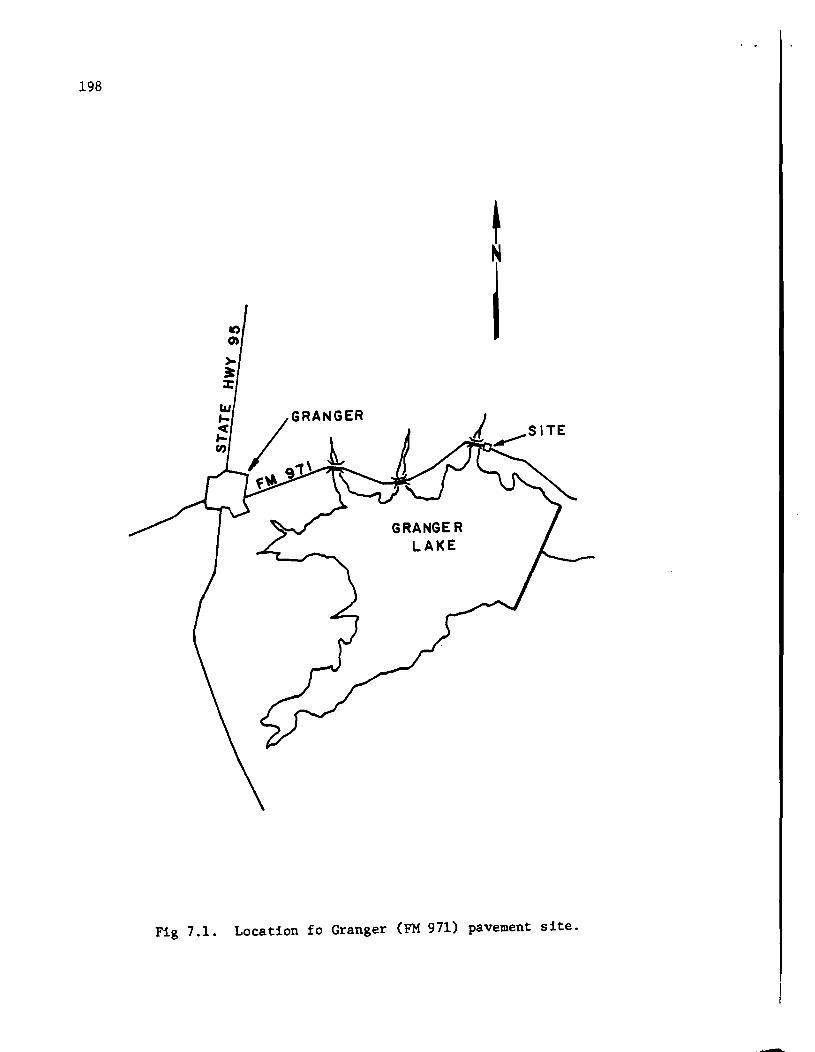
198
GRANGE R LAKE
Fig 7.1. Location fo Granger (FM 971) pavement site.
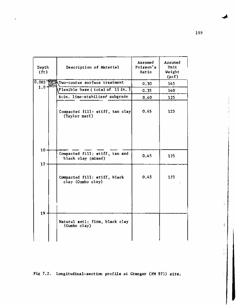
Depth (ft)
Description of Material Assumed
Poisson's Ratio
Assumed Unit
Weight (pcf)
0.08S-~\Two-course surface treatment 0.30 145 1 O-~\~--~~~--~---~~~~~~~---------4---------~
• ~F1exible base ( total of 11 in. ) 0.35 140
10
12
6-1n. 1ime-stabi1ize~ subgrade 0.40 125
Compacted fill: stiff, tan clay (Taylor marl)
- - - -Compacted fill : stiff, tan and
black clay (mixed)
Compacted fill: stiff, black clay (Gumbo clay)
0.45 125
0.45 125
0.45 125
19~~--------------------------------~---------___ ~------~ Natural 80i1: firm, black clay
(Gumbo clay)
Fig 7.2. Longitudinal-section profile at Granger (PM 971) site.
199
200
EXPERIMENTAL PROCEDURE
The procedure used at the Granger site was similar to the procedure used
at the IH 35 site and followed the general procedure discussed in Appendix A.
The drop hammer was the only source of input energy used at the Granger site.
Based on the results from the testing conducted at IH 35, which showed that
horizontal geophones are too sensitive to undesirable P-wave energy, only
vertical geophones were utilized. The geophones were mounted on steel blocks
which were then epoxied to the pavement surface to permit adequate coupling.
Measurements were made with the geophones located along the centerline
of the road and along the right (exterior) wheelpath of the eastbound lane.
Table 7.1 contains a listing of the measurements including the distance from
the source to the geophones and the bandwidth used for each measurement.
Measurements along the centerline included a series of geophone spacings with
the near geophone located 1 ft (0.3 m) from the source and a series of
geophone spacings with the near geophone located midway between the source
and the far geophone. Hereafter, measurements will be referred to by the
location of the geophones from the source.
In addition, deflection readings were obtained from the Dynaflect device
which was made available by the Texas State Department of Highways and Public
Transportation (SDHPT). Measurements were performed at four locations along
both the centerline and the right wheel path. Data were collected at
distances of 53, 78, 103, and 128 ft (16, 24, 31, and 39 m) from the bridge
abutment. Results of these tests are presented herein.

TABLE 7.1. SUMMARY OF MEASUREMENTS AT TIlE GRANGER (FM 911) SITE
Record lifo. Diat.nce fr~ Dhhnce Loc.tion flwlber B.ndwidth (Tract lifo.) Sourc. to betwe.n of of of
C.ophone. (ft) Ceophone. Ceophone. Aver •• e. Spectl'_ .... 1' r.r (tt) (H&)
5(1) 0.5 1.0 0.5 Centerline of Ro.d 5 3200
14(1) 1.0 2.0 1.0 .. II II 5 1600
19(1) 1.0 2.0 1.0 II " " 5 100
24(1) 1.0 2.0 1.0 " " " 5 400
2'(1) 1.0 2.0 1.0 .. " " 5 lZOO
:nU) 1.0 5.0 4.0 tt .. II 5 800
38(1) 1.0 5.0 4.0 " " " 5 400
4'(1) 1.0 9.0 8.0 tt " .. 5 400
44(1) 1.0 9.0 8.0 II " II 5 SO
50(1) 1.0 16.0 15.0 " " " 5 200
55(1) 8.0 16.0 8.0 .. " " 5 200
60(1) 4.0 8.0 4.0 " .. " 5 400
67(1) 2.0 4.0 2.0 to " .. 5 400
74(1) 5.0 9.0 4.0 " .. " 5 400
5(2) 5.0 9.0 4.0 Ritbt Ext. Wheel P.th 5 400
10(2) 1.0 5.0 4.0 . .. .. .. .. 5 800
15(2) 1.0 2.0 1.0 .. II .. .. S 1600
20(2) 7.0 15.0 8.0 " It .. .. S 400
COIIpUter D.t. 'U.
Identification
IRGltl
SIIGIt6
----
SHGtt7
SBClt.8
-IBGl.9
8RGIl4
SHGttl
SRGlt2
SHORS
SHOUt
SRGUI
SHGRIO
SHGR13
I
N o .....

202
DETERMINATION OF VELOCITY PROFILE
For comparative purposes, cross spectrum measurements were divided into
three groups: measurements along the centerline of the road with the near
geophone located midway between the source and far geophone, measurements
along the centerline of the road with the near geophone fixed at a distance
1 ft (0.3 m) from the source, and measurements along the right whee1path.
Velocity profiles obtained from these three sets of measurements are shown in
Figs 7.3, 7.4, and 7.5, respectively. These profiles include data over the
entire frequency range for which interpretable phase information existed,
regardless of the level of coherence for the measurements.
The velocity profiles shown in Figs 7.3 and 7.5 indicate that the R-wave
velocity in the subgrade ranges from approximately 400 to 450 fps (120 to
140 m/sec) for measurements along the centerline of the road as well as along
the whee1path. However, the velocity profile shown in Fig 7.4 indicates that
the R-wave velocity in the subgrade is somewhat higher, ranging from ;50 to
700 fps (140 to 215 m/sec). This large difference is not a result of varying
soil properties since the profile shown in Fig 7.3 represents the same
centerline location. The difference is most likely related to the location
of the pair of geophones, particularly the geophone nearer to the source. In
the case where the near geophone is fixed close to the source (Fig 7.5>,
there is not a sufficient distance for the long wavelengths which sample the
subgrade (LR greater than about 6 ft, (2 .» to disperse, i.e., separate and
travel at a velocity commensurate with the material that the full wavelength
would sample. As a result, the low-frequency waves are influenced
disproportionately by the material near the surface. For pavement systems,
the materials near the surface have higher velocities (more stiffness) than

VELOC I TY, FPS -10 0 25 50 75 100 125
0
" ·T l!i IDI 'II. --
Surface Layer l!JeJ
Base ~(!) (!) J~ rat I!J
'1,Cl ..... IlIA (!)
Stabilized • 6 (!) I!J.I] (§I (!)
Subgrade 6 l!J C+ (!) ~
+ + ,. (. +"m + .......... +1-+
Subgrade- + (!) (!) dB ("II Compacted FUI + (!) (!)
(!)
oft. (!)
+ +6(!)
+ I- 6 u..(1") +
+ 6(!) •
J: I- 6 0-W + 0" 6 (!)
(!)
+ 6
Measurement
0 V\-Vl 0 V2-V4 ll. V4-V8
+ V8-V16
+
Fig 7.3. Unfiltered velocity profile for measurements along the centerline using equally spaced geophones.
203

204
VELCJCITY. FPS -10 a 20 40 60 80 100
0
" Surface Layer
Base III [!Je
[!J [!J [!J F
- Stabilized Am Subgrade
t9 .. Subgrade- ~.. [!J
N Compacted Fill (!)t [!J
.. rP q [!J
...... [!J
lL.(r') ~ [!J
• .. ::c (!) ...... [!J Q...
W .. 0·
(!)
.. (!)
Measurement [!J
0 Vl-V5 .. 0 Vl-V9 (!) ~ Vl-V16
CD
Fig 7.4. Unfiltered velocity profile for measurements along the centerline using a reference geophone located 1 ft from the source.

VELOCITY, o 20 40
FPS -10 60
o Surface Layer ~ I%! t£i ill!)
m ctP (!)
.... Base
Stabilized Subgrade
Subgrade-N Compacted Fill
• :r: fa.. l/..J 0 ....
(!)
1!> l!I
~ A
A m (!)A
m +
(!) Am
80
+ Measurement
(!)
o VI-V2 o Vl-V5 b. V5-V9 + V7-V15
100
Fig 7.S. Unfiltered velocity profile for measurements along the right wheelpath.
205

206
thp. subgrade. Consequently, the apparent subgrade velocity will be higher
than it should be when the near geophone is located an adequate distance from
the source. This phenomenon is observed in Fig 7.4. The problem is
minimized by locating the near geophone at an increasing distance from the
source to sample increasing wavelengths (depths), such as shown in Fig 7.3.
All of the velocity profiles show considerable scatter within 2 ft
(0.6 m) of the surface. The upper part of the profile contains several
relatively thin layers having significantly different properties. For
example, the layer boundary between the surface and the base course can be
observed by the line of velocities plotted at about 0.1 to 0.15 ft (3.0 to
4.6 cm). This layer boundary is clearly shown in Fig 7.3 and is partially
developed in Fig 7.5. However, the layer boundary between the base course
and the subgrade can only be estimated. Because the section of
lime-stabilized subgrade probably has a stiffness between that of the
underlying nonstabilized subgrade and the overlying base course, the
transition between layers is difficult to define.
The scatter in the upper part of the velocity profile is probably due to
the presence of layering which causes some wavelengths to be reflected or
~efracted at layer boundaries. Reflected and refracted waves may influence
the phase of the cross spectrum and, in turn, may complicate the
interpretation of velocities which are based on direct travel distance
between the geophones on the surface.
In general, the phase plots obtained at the Granger site were quite
difficult to interpret. A typical example of the difficulty is shown in
Fig 7.6a for measurement V4-VB. OVer the range of frequencies from about 100
to 200 Hz, various ·'glitches" occur in the phase plot which are not normally
expected in a more continuous relationship such as that shown over the range

180~----~--------~------~~----------------~--~
-180-r----~----~--~~----~--~~--__ ----__ ~~~ 400
(a) Phase of the cross spectrum.
1.01n~------~~~'-------------~----~~----------------~
O.O~----~----,---~~----p---__ ~--__ ----__ --~--J o Frequency, Hz
(b) Coherence function.
Fig 7.6. ~elationship between phase of the cross spectrum and coherence for measurement V4-VS.
400
207

208
from 10 to 100 Hz. In particular, there appears to be a 360-degree phase
shift at about 134 Hz, similar to the shifts occurring at about 53 and
207 Hz. (These shifts are usually a plotting phenomenon; see the discussion
in Appendix A.) However, if the apparent shift at 134 Hz is interpreted as a
360-degree shift, the velocities obtained for frequencies above 134 Hz are
much too low for the base material which those frequencies (or wavelengths)
supposedly sampled. In this case, the sharp break in continuity is due to
actual behavior (rather than just a plotting phenomenon) of waves having
frequencies in the neighborhood of 134 Hz.
The coherence function for measurement V4-V8, shown in Fig 7.6b,
exhibits a sharp spike of poor coherence at 134 Hz which corresponds exactly
to the sharp break in phase shown in Fig 7.6a. In addition, there is another
wider spike of poor coherence at approximately 182 Hz. Analysis of the
reduced data indicates that both of these frequencies correspond to sharp
demarcations in velocities.
Further examination of phase plots and coherence functions from other
measurements revealed that similar spikes or depressions of poor coherence
occurred over frequency ranges where the phase was atypical and/or difficult
to interpret. The sharpness of the spike or depression, as well as the level
of coherence, varied somewhat from measurement to measurement. However,
regardless of the location of the geophones, each measurement showed poor
coherence at the same frequency or range of frequencies (within the
measurement bandwidth). In each case, the frequencies corresponded to sharp
demarcations in velocities. These frequencies and the approximate depths
associated with the velocity contrasts are summarized in Table 7.2. In turn,
it was found that these depths correlate quite closely with layer boundaries
in the profile. This suggests that reflection and refraction of certain

TABLE 7.2. RELATIONSHIP BETWEEN FREQUENCIES WITH LOW COHERENCE AND DEPTH OF LAYER BOUNDARIES
Measurement
V\-Vl
V\-Vl
V2-V4
V4-VS
V4-V8
VS-V16
V1-V16
V1-V2 (WP) * V5-V9 (WP)
V7-V15 (WP)
Frequency
(Hz)
1750-2100
550
183
182
134
105-135
105-115
1225+
185-240
105-110
Approximate Depth** (ft)
0.14-0.18
0.4
1.0
1.0
1.5
1.55
1.5
0.14
1.0
1.55
* Measurements in wheel path denoted by (WP).
Layer Boundary
surface course / base course
1st lift / 2nd lift of base
base / stabilized subgrade
" " " stabi1iEed sub grade / subgrade
" " " " " "
surface tourse / base course
base / stabilized subgrade
stabilized Bubgrade / subgrade
** Depths based on LR/3 criterion; LR is ~avelength for particular frequency.
N o \0
210
waves due to layering does influence the phase of the cross spectrum as well
as the coherence function.
Although measurements with poor coherence are not deSirable, it may be
advantageous, when possible,
coherence to identify layering.
phase of the cross spectrum
to use the spikes or depressions of poor
Such a possibility is shown in Fig 7.7. The
for measurement ~-Vl, shown in Fig 7.7a,
exhibits a broad peak from about 1700 to 2300 Hz. The presence of the peak
indicates that the phase is decreasing although the frequency is increasing.
As the phase decreases, the time for the wave to travel between the geophones
decreases, and the velocity increases significantly. The sharp change in
velocity suggests the influence of a layer boundary. Figure 7.7b shows the
coherence function for the measurement, and, as could be expected, there is a
marked drop in the level of coherence over the frequency range of the peak in
Fig 7.7a. The detection of layers using frequencies may also be enhanced by
examining the magnitude of the cross spectrum plotted on a logarithmic scale
as in Fig 7.7c. Small but distinct dips in magnitude can be observed at
1900 Hz (corresponding to the coherence function) as well as at 550 Hz. This
latter point is barely distinguishable in the phase plot (Fig 7.7a) and is
not well-defined in the coherence function (Fig 7.7b) in view of the fact
that several similar short spikes of poor coherence also exist up to about
1000 Hz. The sensitivity of the logarithmic scale to small dips in magnitude
shows the dip at 550 Hz, whiCh corresponds to a depth of about 0.4 ft, or
about 5 in. (12 em). This depth appears to correspond to the boundary
between the first and second lifts of the base cour8e. Since the material
properties (and, hence, the velocities) are essentially the same in both
lifts, no distinction is observed in the phase plot.
· .

· .
'.' r
180
-III ell ell tiD ell Q\ ~ "cbO g,. ell
'" ......
-180 0 Frequency t Hz 3000
(a) Phase of the cross spectrum.
1.0
ell U C ell
'"' ell
-a u
0.0 0 Frequency, Hz 3000
(b) Coherence function.
10-5~--~----~--------------------~----------------
See Table 7.2
N =: o o Q\ ....
10-l1-P------~------~------~----~~------._----~ o Frequency, Hz 3000
(c) Magnitude (logarithmic scale) of the cross spectrum
Fig 7.7. Detection of layer boundaries using spectral measurements.
211

212
Although the major layer boundaries can be approximated, there is still
the problem of assigning a velocity to the base course, where excessive
scatter exists in the data (Figs 7.3-7.5). For soil sites, such scatter
could be identified and filtered out using the criterion developed in
Chapter 4. For pavement sites, a general equation (such as Eq 4.5) cannot be
readily applied because the various materials have significantly different
properties. However, the same approach can be applied; data for frequencies
with poor coherence are rejected and thereby filtered out of the velocity
profile. The definition of "poor" coherence is somewhat arbitrary. Analysis
of the various measurements indicates that data for which y2 < 0.90 should
be filtered out.
Using this criterion, the velocity profiles were filtered and replotted.
Figure 7.8 shows the profile to a depth of 7 ft (2.1 m) for measurements
along the wheelpath. Figure 7.9 shows the profile to a depth of 14 ft
(4.3 m) for measurements along the centerline. Both profiles still show some
scatter, which is probably remnant of the reflection and refraction problems
previously discussed. The transition zone is still present at the depth of
the stabilized subgrade.
Rayleigh wave velocities can be determined for the subgrade and the base
using Fig 7.8, and R-wave velocities can be determined for the subgrade, the
base, and the surface layer using Fig 7.9. A "mean value" for the velocity
in each layer was selected by graphically fitting a straight line through the
data which are least influenced by the layer boundaries. In the subgrade, a
velocity of 420 fps (128 mlsec) was obtained from measurements along the
wheelpath and a velocity of 440 fps (134 m/sec) was obtained from
measurements along the centerline, yielding an average value of 430 fps
(131 m/sec). In the base course, a velocity of 680 fps (207 m/sec) was

..
VELOCI TY. FPS -10 0 20 40 60 80 100
c Surface Layer
tf>(!) (!) ~ Base ~ (!) - (!) • Stabilized
(!),~ .. Subgrade ..... (!) ...
Subgrade- .. ~(!) t!l
N Compacted Fill ~
~
t ..... +; lL.(I')
l> .. J: Cf" ..... (L
W .. 0" ..
...
.. ... Measurement
0 vt-V2 + 0 VI-V5 ..
6- VS-V9 ... + V7-V15 CD
+
..
Fig 7.8. Filtered Rayleigh wave velocity profile for measurements along the right wheel path.
213

214
VEL(jCITY, FPS -10 0 2 4 60 80 100
c \ Surface Layer Base Stab. Subgrade *' •
N Subgrade- (!)
~ • (!) Compacted Fill +~ (Taylor Marl) : I.. +
+ I.. (!) •
+ • + •
... I-LLw
+ • ::c Measurement
l- • + a... 0 V\-Vl W 0 V2-V4 OCD + ~ V4-V8
+ + VS-Vl6
+ X Vl-V9 • 0 Vl-Vl6
+ c :a + - + +
Compacted Fill "i (mixed)
• +
N -Compacted F 11 1 • (Gumbo Clay)
• • -
Fig 7.9. Filtered rayleigh wave velocity profile for measurements along the centerline.

· '
215
obtained from measurements along the wheel path and a velocity of 660 fps
(201 mlsec) was obtained from measurements along the centerline, yielding an
average value of 670 fps (204 mlsec). The velocity in the surface layer was
determined from centerline measurements only and was estimated to be 980 fps
(299 mlsec).
The subgrade velocity obtained from cross spectrum measurements can be
compared with crosshole velocities obtained by Long (1980) immediately after
the construction of the embankment. Long obtained shear wave velocities 1n
the fill material ranging from about 515 to 530 fps (157 to 162 mlsec). From
cross spectrum measurements, the R-wave velocity of 430 fps (131 m/sec)
converts to an S-wave velocity of 453 fps (138 mlsec) for a clay with
Poisson's ratio of about 0.45. Thus, the S-wave velocity from cross spectrum
measurements is about 15 percent lower than the 5-wave velocities from
crosshole tests. Since the cross ~pectrum measurements were made after a
period of wet weather, the lower velocities may reflect a greater moisture
content than when the crosshole tests were performed (several years earlier).
The velocity profile in Fig 7.9 shows a small but marked decrease in
velocity at about 10 ft (3 m). This depth corresponds with the depth at
which the compacted fill aaterial changes from Taylor marl to gumbo clay.
This close correlation between the velocity profile and soil profile suggests
that the LR!3 criterion for depth is appropriate for the Granger site.
Again, the lower velocity below 10 ft (3 m) may be a result of the heavy
rainfall and subsequent increase in elevation of the water table due to
impoundment of Granger Lake. Borings were not performed to obtain samples or
determine water contents at the time the cross spectrum measurements were
made.
216
DETERMINATION OF MODULI
Using the values for R-wave velocities determined from cross spectrum
measurements and estimated values for unit weights and Poisson's ratios,
values for S-wave velocities, shear moduli, and Young's moduli were
calculated for the surface layer, base, and subgrade. These values are
listed in Table 7.3. Young's moduli for the surface layer, base, and
subgrade were determined to be 91,000 psi, 42,000 psi, and 16,000 psi,
respectively. These values fall within the range typical of the respective
materials. In addition, a Young's modulus for the stabilized subgrade was
calculated to be 23,000 psi based on an estimated R-wave velocity.
Moduli were backcalculated (by SDHPT) from Dynaflect data using ELSYM5
as described in Chapter 6. Four layers were assumed, including a surface
course, flexible base, and lime-stabilized subgrade having layer thicknesses
of 1 in., 11 in., and 6 in., respectively, and a subgrade of infinite extent.
The moduli from deflection measurements are listed in Table 7.3. ,These
moduli are considerably lower (by as much as 1/2 to 1/3) than those
calculated from wave propagation velocities.
Deflections were also calculated (by ELSYM5) using the moduli determined
from wave velocities. The calculated deflections were 1.39, 1.20, 0.67,
0.47, and 0.35 mils for locations of 0, 1, 2, 3, and 4 ft from the source.
In comparison, the measured deflections (based on an average for 7 readings)
were 2.27, 1.59, 0.95, 0.61, and 0.44 mils, respectively. The calculated
deflections are approximately 20 to 40 percent lower than the measured
deflections, which would be expected since the moduli from wave propagation
velocities were higher than the moduli found by using ELSYM5.
..

Material Unit Weight
(pef)
Surface 145
Base 140
Stabilized 125 Subgrade
Subgrade 125
TABLE 7.:3. SUMMARY OF WAVE VELOCITIES AND ELASTIC MODULI DETERMINED AT GRANGER (FM 971) SITE
Poisson's R-Wave S-Wave Shear Young's Modulus, E (psi) Ratio Velocity Velocity Modulus Wave Deflection
(fps) (fps) (psi) Propagation Method*
0.30 980 1060 35,000 91,000 50,000
0.35 670 720 15,700 42,000 13,000
0.40 520 550 8,100 23,000 12,500
0.45 430 450 5,500 16,000 12,000
*Modu1i were backcalculated from fitted deflection basin using elastic layer theory (ELSYMS).
N I-' .....,
218
The agreement between the wave propagation method and the deflection
method is not particularly good. The differences in moduli (or deflections)
suggest that the methods are not equivalent or interchangeable. It is
difficult to assess which method is more "accurate." Perhaps the assumptions
of elastic layer theory used in ELSYM5 are not reasonable for older,
deteriorating, or cracked pavements such as the sections at the Granger site.
In contrast, the wave propagation method did provide fairly good correlation
with the profile layering and crosshole velocities at the site.
SUMMARY
Analyses of the cross spectrum measurements made at the Granger pavement
site were generally more difficult to interpret than measurements made at the
Austin pavement site.
velocity profile in
In particular, there was significant scatter in the
the surface layer and base course. Examination of the
coherence function, along with erratic patterns in the phase of the cross
spectrum, indicated that marked depressions or spikes of low coherence
occurred at frequencies whose wavelengths corresponded to depths of layer
boundaries. Identification of these frequencies and layer boundaries
permitted better interpretation of the cross spectrum phase plots.
Much of the scatter was reduced by filtering out data for frequencies
which displayed a value of coherence less than 0.90. Also, data were not
used for which the wavelengths were too long to sample effectively an
appropriate depth of material (when the geophones were located too close to
the source). The filtered velocity profile correlated well with the site
profile. The S-wave velocity for the 8ubgrade was about 15 percent lower
than that obtained from crosshole tests performed during the construction of
· .
· .
219
the embankment, possibly because the cross spectrum measurements reflected a
greater moisture content following a period of wet weather.
Young's moduli obtained from the wave propagation velocities were
considerably greater (up to 2 or 3 times) than those backcalculated from
deflection measurements using ELSYM5. Conversely, deflections using moduli
from the wave propagation method were 20 to 40 percent less than the measured
(Dynaflect) deflections. Inasmuch as the cross spectrum measurements
provided a velocity profile which correlated closely with the site profile
and crosshole velocities, the differences in moduli between the two methods
suggest that the elastic layer theory used in ELSYM5 may not apply well to
thin, surface layered pavement.


CHAPTER 8. SUMMARY, CONCLUSIONS, AND RECOMMENDATIONS
SUMMARY
A method to determine elastic moduli at soil and pavement sites was
proposed and tested. Criteria which guided the development of this method
included the restraint of non-destructive testing, accuracy of moduli for all
layers regardless of thicknesses, and quickness and efficiency for rapid,
extensive testing. To meet these criteria, surface receivers were utilized
to evaluate the Rayleigh-wave motion created by a vertical impulsive source
that could excite a wide range of frequencies with a single impact. Analysis
was facilitated by using a portable spectral analyzer to study the magnitude
and phase of the frequency content of the recorded wave pulse.
Phase information from the cross spectrum function was used to calculate
Rayleigh wave velocities which were converted to shear wave velocities.
Elastic moduli (shear ~odull and Young's moduli) were then calculated from
the shear wave velocities. Results from field testing at two pavement sites
and two soil sites indicate that the spectral analysis of surface waves
provides an accurate estimation of the velocity (and, hence, modulus) prof tIe
of a site. The following sections present general conclusions regarding
test-related variables, as well as specific conclusions and recommendations
particular to testing at eoil sites and pavement sites.
J
222
GENERAL CONCLUSIONS REGARDING TEST-RELATED VARIABLES
Several transient events, or impacts, should be averaged together to
obtain a representative cross spectrum measurement. The number of averages
may vary somewhat with the reproducibility of the source, but, typically five
averages will provide a representative measurement. Additional averages do
not seem to improve the measurement sufficiently to warrant the extra testing
time.
Several sources were investigated. Results show that the stress (or
strain) level is not necessarily the critical parameter for selecting an
appropriate impact hammer. Selection should be based on the range of
frequencies that can be sufficiently excited to sample the site profile
adequately. Energy of excitation should not be focused on a few frequencies
but should be distributed over all frequencies in the bandwidth. On this
basis, a light hammer producing a sharp impulse is much more suited than a
large weight which produces a relatively "cushioned" illlpulse, particularly
for testing pavement sites.
Signals recorded with velocity transducers, or geophones, appear to
provide valid cross spectrum measurements up to frequencies of at least
3 KHz. Based on tests performed on pavements, vertical geophones provide a
more accurate R-wave velocity profile than horizontal geophones. Velocities
obtained from measurements using horizontal geophones were generally too
high, probably due to the greater sensitivity of horizontal geophones to the
higher velocity P-waves.
The spacing of the geophones from the source also is illlportant. In
general, an "equally spaced" arrangement, where both the near geophone and
the far geophone are located at increasing distances from the source, is more
• >

- ------------------------------
223
desirable than a "reference" arrangement, where the near geophone is fixed at
a location close to the source and only the far geophone is located at
increasing distances from the source. The former arrangement provides a more
accurate velocity profile, particularly at greater depths (greater
wavelengths) • The equally spaced arrangement appears to be better than the
reference arrangement because the near geophone is located at a sufficient
distance from the source, which allows the different frequencies to disperse
(by travelling at different velocities) as well as permitting the longer
wavelengths to travel through a depth of material which the wave(s)
supposedly sampled.
Velocities for given frequencies were assigned to depths from wavelength
criteria corresponding to an "effective sampling depth" of material
properties. Based on comparisons with S-wave velocity profiles from
crossho1e testing, a depth criterion of ~/3 provided a velocity profile
which correlated best with the crosshole profile. Velocities from cross
spectrum (surface) measurements did not differ from crosshole velocities by
more than 20 percent in the extreme and were typically within less than 10
percent. Inasmuch as crosshole data did not exist for depths greater than
30 ft (9 m), it is not certain if the LR/3 criterion is applicable for long
wavelengths.
The surface technique is restricted to using an average velocity and the
determination of a velocity profile based on wavelength criteria is somewhat
empirical. The problem of averaging is particularly evident at layer
boundaries. Although the empirical approach provides reasonably good
correlation with the site profile and crosshole data, it is desirable to
incorporate a more rigorous and "accurate" approach for determining the
velocity profile from surface measurements. Such an approach involves

224
Rayleigh-wave inversion and extensive n\DDerical techniques to "back out" the
velocity (or modulus) profile and to eliminate or minimize the problems
associated with averaging. This approach could be used to refine the
analysis of measurements from surface testing.
In addition to the cross spectrum function, other functions may be
helpful in the analysis of data. The coherence function is most definitely
needed to assess the range of frequencies over which quality data were
obtained for a given measurement. The linear spectr\DDs or autospectr\DDs can
indicate which frequencies are adequately excited to measure a good response.
Lastly, the transfer function may be used to calculate attenuation properties
at a site.
CONCLUSIONS AND RECOMMENDATIONS FOR SOIL INVESTIGATION
For typical soil sites, frequencies up to about 100 to 200 Hz should be
excited. For depths greater than about 25 to 30 ft (7.6 to 9.1 m), the
measurement bandwidth should be reduced to at least 2S Hz to obtain adequate
resolution of low frequencies. Geophones with low resonant frequencies, or
perhaps accelerometers, should be used to obtain a "flat" transducer response
over the range from 0 to 10 Hz.
The source should be adequately coupled with the soil to ensure transfer
of wave energy over the necessary range of frequencies. The source should
also be large enough to excite low-frequency waves sufficiently enough to
sample depths well below the surface. For depths to about 30 ft (9 m), the
drop hammer appears to be adequate. For greater depths, a larger source IS
desirable to provide sufficient energy at low frequencies. This additional
..
225
wave energy would also permit greater spacing of the geophones from the
source, which is necessary to sample the longer wavelengths accurately.
Testing should include a series of various geophone spacings so that all
wavelengths are accurately sampled during at least one measurement. For
spacings close to the source, short wavelengths will be accurately sampled
but long wavelengths will not have travelled a sufficient distance to measure
properties to an adequate depth. Conversely, for spacings farther from the
source, long wavelengths will be accurately sampled but short wavelengths may
have attenuated too much for a valid frequency response to be obtained.
Based on the coherence function, criteria can be established for a given site
whereby inappropriate wavelengths (or frequencies) can be filtered from the
velocity profile. Filtering reduces much of the scatter in the data, and
using a series of measurements, will result in some overlap in the profile.
This overlap of several measurements provides a more-representative profile
than a single measurement would permit.
Attenuation and damping data were calculated from transfer function
measurements. The coefficient of attenuation a for Rayleigh waves could be
approximated as a linear function of frequency. Values of damping ratio were
calculated from a and ranged from about 8 to 20 percent, depending on the
particular site. These values are somewhat higher than those typically
measured with laboratory samples. Possible reasons for the higher in situ
values may be that the field measurement may have erroneously interpreted
geometrical damping of body wave energy as material damping and/or the field
measurement accurately reports backscattering of wave energy caused by
material anomalies, voids, reflections, or refractions. The former problem
could be resolved by locating the near geophone at 8 to 10 ft (2.4 to 3.0 m)
from the source, thereby allowing adequate distance for the geometric damping

226
of body waves. Results from this investigation certainly show potential
application of spectral analysis in the determination of attenuation and
damping.
CONCLUSIONS AND RECOMMENDATIONS FOR PAVEMENT EVALUATION
For pavement sites consisting of a flexible (AC) surface, frequencies up
to 2 to 5 kHz should be excited. This upper bound will vary depending on the
thickness and stiffness of the surface layer. Higher frequencies are
necessary for thinner, stiffer pavements. Based on tests at two pavement
sites, it appears that geophones provide good response up to at least 3 kHz.
For higher frequencies, it may be necessary to use accelerometers.
Cross spectrum measurements should be made for a series of various
geophone spacings from the source so that all wavelengths can be accurately
sampled. Spacings close to
frequencies, which sample
farther from the source are
sample the
measurements
subgrade. By
will occur,
the source are better for measuring higher
the surface layer and base course • Spacings
better for measuring low frequencies, which
using
which
a series of spacings,
will minimize the
some overlap of
possibility of
misinterpreting reflections or refractions of waves at layer boundaries. The
coherence function should also be used in conjunction with the cross spectrum
to identify poor data. Spikes or depressions of low coherence may be
associated with layer boundaries, and their identification may be helpful in
analyzing the phase of the cross spectrum.
Comparisons between moduli calculated from wave propagation velocities
and moduli backcalculaed (by ELSYK5) from measured Dynaflect deflection
basins indicate that the wave propagation method is a valid method to

227
determine Young's modulus for each layer in a pavement system. Agreement
between the two methods was quite good at the Austin site, where the pavement
was newly constructed, but was not as good at the Granger site, where the
pavement was several years old and showed signs of deterioration. The poorer
comparison at the Granger site may result from assumptions in the elastic
layer program that are not reasonable for thin layered pavement. In general,
it is not clear how applicable the elastic layer theory incorporated into
ELSYK5 is for low-strain (less than 0.001 percent) dynamic loading.
Shear wave velocities in the subgrade obtained from surface measurements
correlated well with those obtained from crosshole testing, suggesting that
the spectral analysis (surface) method is not hindered by the relatively
stiff asphalt layer at the surface. However, both of the pavement systems
investigated in this research consisted of flexible surface layers, with
stiffnesses about 5 to 10 times those for the subgrade. For rigid (PC)
pavements, the stiffness of the surface layer is considerably greater and may
complicate the analysis of subgrade velocities and moduli. Further research
is necessary to determine if the surface method is applicable for rigid
pavements.


REFERENCES
1. Ballard, R. F., Jr., "Determination of Soil Shear Moduli at Depth by
In-Situ Vibratory Techniques;' WateTwaya. Experiment Station, Misc.
Paper No. 4-691, December 1964.
2. Ballard, R. F., Jr •• and D. R. Casagrande, "Dynamic
Investigations, TAA-2A Radar
Waterways Experiment Station, Misc.
1967.
Site, Cape Kennedy,
Paper No. 4-878,
Foundation
Florida, ..
February
3. Bahn. A., P. Ullidtz, R. Stubstad, and A. Sorenson, "Danish Experiments
with the French Falling Weight Deflectometer," Proceedinss, Third
International Conference on the S~cuctural Design of Asphalt
Pavements, Vol. 1, pp 1119-1128, 1972.
4. Bolt, B. A., Nuclear Explosion! and Earthquakes, W. H. Freeman and
Company, San Francisco, California, 197~.
5. Brigham, E. 0., The!!.!E.. Fourier Transform, Prentice-Hall, Englewood
Cliffs, New Jersey, 1974.
6. Ewing, W. M., W. S. Jardetzky, and F. Press, Elastic Waves in Layere~
Media, McGraw-Hill Book Company, New York, 1957.
7. Fry. Z. B., -Developaent and EvaluatLon of Soil Bearing Capacity.
Foundations of Structures," Waterways Experbaent Station, Technical
Report No. 3-632, Report No.1, Julp 196..1.
229

230
8. Heukelom, W., "Auscultation Dynamique de Constructions Routieres," La
Propagation des Ebranlements dans les Milieux Heterogenes,
Colloques Internationeaux du Centre National de la Recherche
Scientifique, No.
1961.
111, Marseille, France, pp 129-141, September
9. Heukelom, W., and C. R. Foster, "Dynamic Testing of Pavements," Journal
of the Soil Mechanics and Foundations Division, American Society of
Civil Engineers, Vol. 86, No. SMl, pp 1-28, February 1960.
10. Hewlett-Packard Company, "Digital Signal Analysis - Time and Frequency
Domain Measurements," Application Note 240-0, Hewlett-Packard,
August 1977.
11. Hoar, R. J., "In Situ Seismic Velocity and Attenuation Measurements for
Dynamic Analyses," Ph.D. Dissertation, The University of Texas at
Austin, 1981.
12. Hoar, R. J., and K. H. Stokoe, II, "Generation and Measurement of
Shear Waves In Situ," Dynamic Geotechnical Testing, ASTM STP 654,
American Society for Testing and Materials, 1978.
13. Jones, R., "Surface Wave Technique for Measuring the Elastic Properties
and Thicknesses of Roads: Theoretical Development," British
Journal of Applied Physics, Vol. 13, pp 21-29, 1962.
14. Kudo, K., and E. Shima, "Attenuation of Shear Waves in Soil," Bulletin
of the Earthquake Research Institute, Vol. 48, Part 2, pp 145-158,
March 1970.
15. Long, L. G., "Comparison of Field and Laboratory Dynamic Soil
Properties," Master's Thesis, The University of Texas at Austin,
1980.

231
16. Lytton, R. L., W. M. Moore, and J. P. Mahoney, Pavement Evaluation:
Phase I Pavement Evaluation Equipment, Report No. FHWA-RD-75-78,
Federal Highway Administration, Washington, D. C., 1975.
17. MeDonal, F~ J., F. A. Angona, R. L. Millis, R. L. Sengbush, R. G. Van
Nostrand, and J. E. White, "Attenuation of Shear and Compressional
Waves in Pierre Shale," Geophysics, Vol. 23, pp 421-439, 1958.
18. Miller, G. F., and H. Pursey, "On the Partition of Energy Between
Elastic Waves in a Semi-Infinite Solid," Proceedings Royal Societ~,
London, Series At Vol. 233, pp 55-69, 1955.
19. Newland, D. E., Random Vibrations and Spectral Analysis, Longman,
London, 1975.
20. Patel, N. S., "Generation and Attenuation of Seismic Waves in Downhole
Testing," Master's Thesis, The University of Texas at Austin, 1981.
21. Rao, H. A. B., and D. Harnage, "Evaluation of Rigid Pavements by
Nondestructive Tests," Highway Research Record No. 407: Pavement
Technology, Highway Research Board, pp 76-86, 1972.
22. Rayleigh, Lord, "On Waves Propagated Along the Plane Surface of an
Elastic Solid," London .Mathematical Society Proceedings, Vol. 17,
pp 4-11.
23. Richart, F. E., Jr., J. R. Ball, Jr., and R. D. Woods, Vibrations of
Soils and Foundations, Prentice-Hall, Englewood Cliffs, New Jersey,
1970.
24. Stokoe, K. H' t 11, and R. J. Boar. "Variables Affecting In Situ Seismic
Measurements, M Earthqualu!. En,gineering and §2.!! Dynamics. Vol. II,
American Society of Civ!l Engineers, pp 919-939, 1978.

232
25. Stone1ey, R., "Elastic Waves at the Surface of Separation of Two
Solids," Proceedings of the Royal Society of London, Series A, Vol.
106, pp 416-428, December 1924.
26. Szendrei, M. E., and C. R. Freeme, "Road Responses to Vibration Tests,"
Journal of the Soil Mechanics and Foundations Division, American
Society of Civil Engineers, Vol. 96, SM6, pp 2099-2124, November
1970.

APPENDIX A
DISCUSSION OF EXPElUMENTAL PROCEDUUS AND DATA ANALYSIS
'': '
.. - -. '
~:.~-'~:.~.
';-":-.'."
'.-" ,

" .... ,
. '.
~;: ~~~~.~~ . r:, ~~,;"

APPENDIX A
DISCUSSION OF EXPERIKENTAL PROCEDURES AND DATA ANALYSIS
This appendix outlines the steps involved in the acquisition and
analysis of frequency data to obtain a VS-versus-depth profile. It is
assumed that the reader is familiar with the basic operation of the
Hewlett-Packard 5423A Analyzer.
FIELD PROCEDURE FOR DATA ACQUISITION
Frequency data can be acquired directly in the field with the
Hewlett-Packard 5423A Structural Dynamics Analyzer, shown in Fig A.l. The HP
5423A Analyzer consists of three portable units having a net weight of 115 Ib
(52.2 kg). The three units stack together vertically during operation and
are interconnected by means of appropriate cables. Complete performance
specifications as well as operator instructions are contained in the three
volumes of the Hewlett-Packard 5423A Users' Guide.
Analxzer Set-up
The analyzer .ust be ·programmed" for a particular measurement state.
The format (and typical set-up) of the measurement state is shown in Fig A.2.
The measurement state is displayed in three sections which include:
235
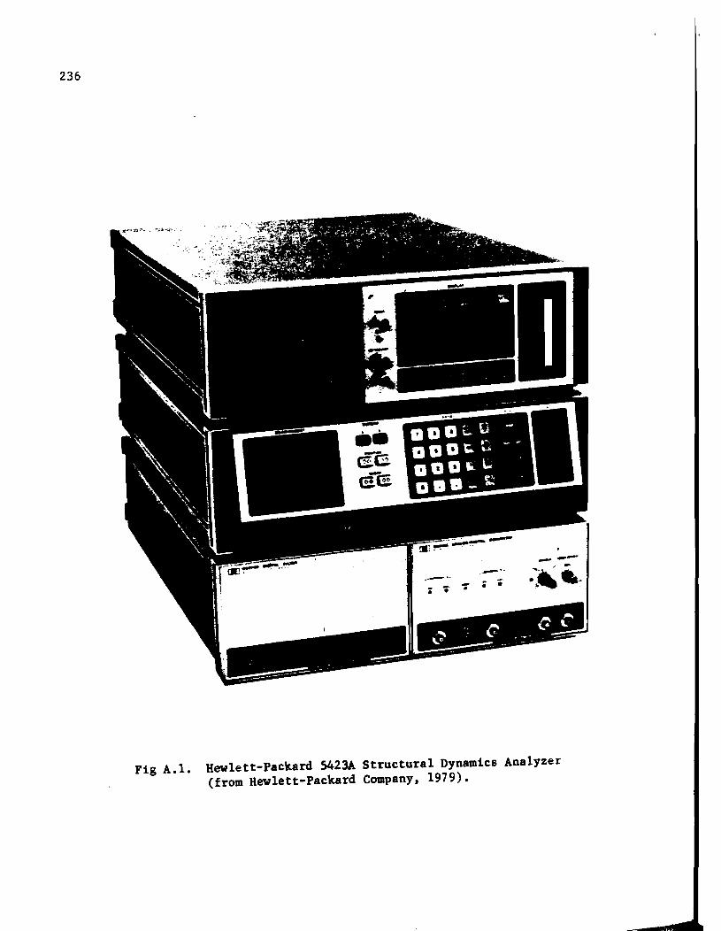
236
Fig A.l. Hewlett-Packard 5423A Structural Dynamics Analyzer (from Hewlett-Packard Company, 1979).

tEASlRENENT STATE
tEASlI9ENT I TRANSFER FlKTI~
AVERAGE I
SIGNAL I
TRIGGER •
CENT FRB1 •
BANlWIDTH I
5
IMPACT
INTERNAL
• STABLE
• OIL 1
AF.
TIME LEMrrH I
8-1 HZ
I ... HZ
2. SIIII1I S AT •
CHAN f
* 1 *2
RAta ACIOC
2.SV DC 2.SV DC
IELAY
-21._ as -2B._ as
2. 5IBIJ as
CAL<BJIV>
1._ 1._
Fig A.2. Format and typical setup of a measurement state.
237

238
(1) the type of measurement and how it will be obtained,
(2) the frequency bandwidth or time length information specified, and
(3) the selected parameters for the analog-to-digital conversion of the input signals.
To obtain data for determining wave propagation velocities, the
measurement should be specified in accord with the following guidelines.
The transfer function should be specified as the desired measurement
although the cross-spectrum measurement would provide the necessary
information. When the transfer function is specified, the analyzer also
provides the coherence function, the cross-spectrum, and the autospectrums of
each input signal. The additional measurements may aid in the subsequent
analysis of the data. As a general rule, five "averages" should be used to
construct the measurement. Stable averaging should be used in order to give
each event in the ensemble equal weight. The signal type should be specified
as "Impact," which allows for the acceptance or rejection of a particular
transient event. In this way, poor impulses can be eliminated from the
overall average.
The trigger type may vary depending on the available equipment. The
most convenient method is simply to trigger internally off the signal going
into the first channel. The trigger level can be adjusted to fix a starting
point (t-0) in the first half sine wave of the impulse as it passes by the
first geophone. A pre-trigger delay must be used to capture the initial
portion of the impulse that would otherwise be lost prior to triggering.
Since only the relative phase between the signals of the two geophones is
required, an external trigger is not necessary.

239
The selection of the measurement bandwidth or time length depends on
several considerations, including the spacing between geophones, the desired
resolution in the frequency spectrum, the attenuation properties of the site,
and the range of wavelengths needed to investigate the site to a desired
depth. The interdependence of these variables is discussed in detail in
Chapter 4. For most soil sites, a bandwidth of 100 to 200 Hz should
adequately cover the range of frequencies needed to "sample" within a foot or
two of the surface. For pavement systems, frequencies from 1.6 to 3.2 Hz may
be required to sample the thin, high-velocity layer at the surface. In each
case the "center frequency" should be specified as zero, so that the
measurement is made in the "baseband" mode, i.e., the bandwidth ranges from 0
to, say, 100 Hz. Note also that the selection of a bandwidth or a time
length automatically establishes the other. Since frequency and period are
inversely related, both bandwidth and time length cannot be specified
independently. Additionally, because the HP 5423A uses a fixed number of
points to digitize the signal, selection of a bandwidth or time length
automatically establishes 6f and 6t, the resolution or precision of the
measurement in the frequency domain and the time domain. respectively.
The parameters pertaining to the analog-to-digital converter (ADC) can
differ between input channels 1 and 2. However, in general, only the range
should differ. The specification of the range for each channel is related to
the voltage output of each geophone. The value for range should be as small
as possible to increase the sensitivity of the ADC. When the voltage output
from the geophone(s) exceeds the specified range, a caution message will
appear: ··ADC OVERFLOW, IMPACT AGAIN." Subsequent signals can be utilized by
increasing the range to an appropriate value (not exceeding + 10 volts). For
both channels, DC coupling should be specified. For measurement of wave

240
propagation velocities, a calibration factor need not be specified as long as
the frequency response curves for each geophone are nearly identical.
Lastly, when triggering internally with the signal from the near
geophone, a trigger delay must be specified. The same trigger delay should
be specified for each channel so as not to introduce an internal time or
phase delay for measurements incorporating both signals. The exact value of
the delay will vary somewhat with the velocity of the material at the site as
well as the distance be teen the source and the near geophone. In general, a
delay of 5 to 50 milliseconds should prove adequate. Note that the delay is
negative, since the pre-trigger (before t-O) portion of the signal is to be
captured.
Measurement Acquisition
Prior to the measurement of the transfer function, the input time
signals should be checked. This can be done before each impact event is
accepted (or rejected) for the measurement ensemble. However, in the case of
narrow bandwidth measurements (say, 100 to 200 Hz), the time signal may be
compressed and/or have poor resolution as shown in Fig A.3a. In such cases,
it is beneficial to perform initially a "time record average" with a
relatively wide bandwidth (say, 1600 Hz) to verify that the geophones are
connected properly to the ADC. This preltminary measurement can be used to
check that the trigger delay 1s appropriate, that the entire transient event
1s being captured, and that both geophones are connected with the same
polarity (i.e., a •• downward" impac t produces an initial downward impulse in
the time signal of both geophones). The benefit of using a wide bandwidth
measurement to check the input signal(s) is shown in Fig A.3b.

0.5 -
"'"' ~ -.-I
~ --""' -:;)
.e- -.J :;) o _ QI C o -.c c.. ~ -c -
-0.5~------~-------r------.-------~------r_----_.~ I I I I I I I o Time, seconds 1.2
1.0
-""' :;)
(a) Narrow-bandwidth (BW = 200 Hz) measurement
fr ~ _______________ -J
:;) o Qj
c o -a o II)
C
-l.O-r-----r----~----~----_.----_.----~r_----r_--~
-20 Time, milliseconds
(b) Wide-bandwidth (BW - 1600 Hz) measurement
Fig A.3. Comparison of time records obtained from measurements with narrow and wide bandwidths.
60
241

242
Once the input time signals have been checked, the transfer function can
be measured. After the measurement is completed, the coherence function
should be examined to confirm that a ·'good" measurement was obtained over the
desired bandwidth. Such a check may indicate that the bandwidth should be
lengthened or shortened to optimize the range or resolution of frequency
information. The range of frequencies providing useful information (good
coherence) will vary somewhat with the distance between the geophones. In
general, wider spacings between geophones will lead to attenuation of high
frequencies. Each new measurement should be checked and adjusted
accordingly.
In addition, the phase of the cross-spectrum should be examined to
confirm that meaningful information has been gathered. Finally, it may be
useful to compare the auto spectrums from each geophone to determine which
frequencies have been excited sufficiently enough to provide good transfer
function data. In particular, the autospectrum from the geophone farthest
from the source may indicate the upper limit of frequencies which can be
excited at that particular distance.
Permanent Data Storage
When a satisfactory measurement has been obtained and checked, each
available function should be recorded on magnetic tape. The available
functions should include the transfer function, the coherence function, the
cross-spectrum, and both autospectrums. Although the two autospectrums could
be used to reconstruct the other three functions, it is most convenient to
save all five functions directly while in the field.
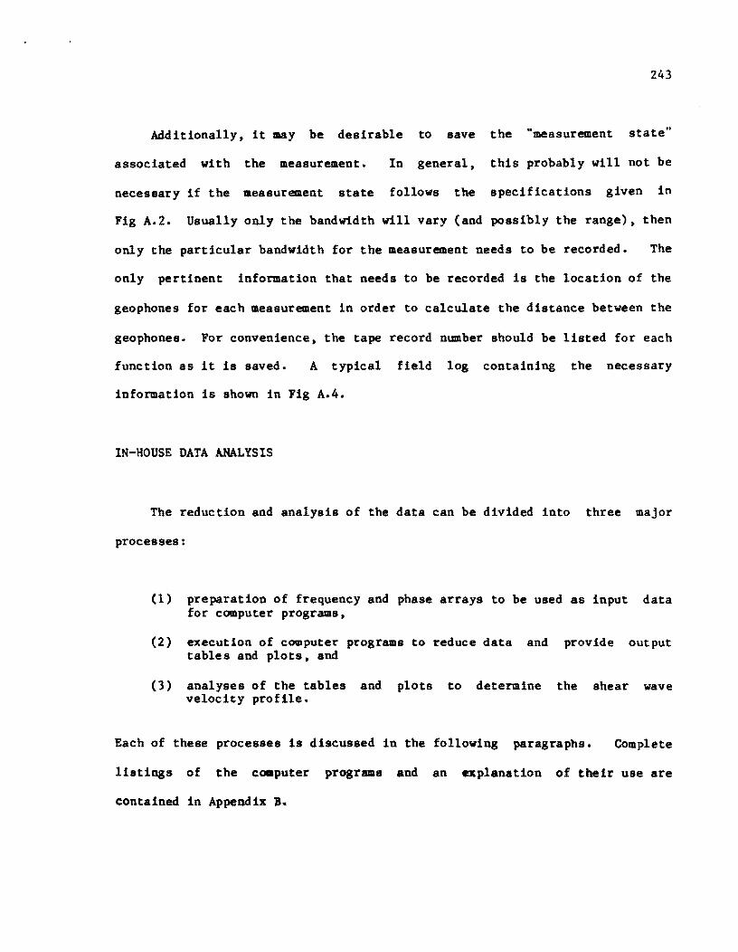
243
Additionally, it aay be desirable to save the "measurement state"
associated with the measurement. In general, this probably will not be
necessary if the measurement state follows the specifications given in
Fig A.2. Usually only the bandwidth will vary (and possibly the range), then
only the particular bandwidth for the measurement needs to be recorded. The
only pertinent information that needs to be recorded is the location of the
geophones for each measurement in order to calculate the distance between the
geophones. For convenience, the tape record number should be listed for each
function as it is saved. A typical field log containing the necessary
information is shown in Fig A.4.
IN-HOUSE DATA ANALYSIS
The reduction and analysis of the data can be divided into three major
processes:
(1) preparation of frequency and phase arrays to be used as input data for computer programs,
(2) execution of computer programs to reduce data and provide output tables and plots, and
(3) analyses of the tables and plots to determine the shear wave velocity profile.
Each of these processes is discussed in the following paragraphs. Complete
listings of the coaputer programs and an explanation of their use are
contained in Appendix B.
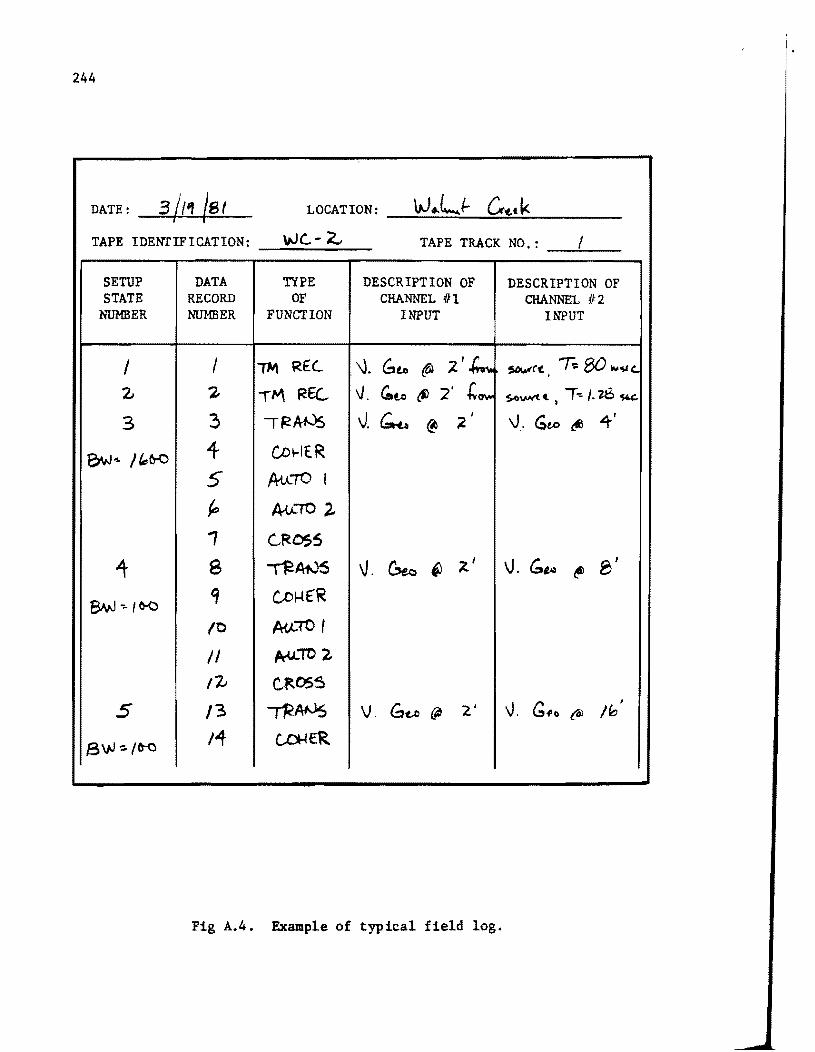
244
DATE: 3/''1 IS I LOCATION: _....;;.W......; ... ;...-L.;.;.;;;:...f-..........;C.:;..;..::.'tt:..;.k~ __ _
TAPE IDENI'IFICATION: _..;;.W_C-_-_2..-__ TAPE TRACK NO,: _...:..' __
SETUP STATE
NUMBER
4
5
DATA RECORD NUMBER
I z 3 4 5 ~
1
8 ~
(0
/I /2
/3
14
TYPE OF
FUNCTION
'TIll {<.£c..
TM r<EC..
if2MJs
GDI-IER
~TO I
M;../O 2-
G~O$~
-r12A1J5
GDI-{~
~-rol
A-U-i02
~fie.055
'Tf2AtJS ~ER
DESCRIPTION OF CHANNEL :(il
INPUT
\). Gtto (6J ~'~
V, G.t.o €1J 2' '-ow V. 6.u @ ~'
V. G'Ul @ 2'
Fig A.4. Example of typical field log.
DESCRIPTION OF CHANNEL ff2
INPUT
~(C. I T-= 80 .... '!l (. $OvNtt. T-:./. zb ~
I
'V_, Ge-o ~ 4 I

245
Preparation of Data Arrays
The computer programs are designed to convert phase data to velocity and
wavelength information for selected frequencies. Currently, the input arrays
are dimensioned to handle 50 pairs of frequency and phase data (f,e).
The selected frequencies can range over the entire bandwidth for which
the measurement was obtained. However, in general, the selected frequencies
should not be evenly distributed over the bandwidth if a well-distributed
velocity profile is desired. More concentration should be given to the lower
frequencies (about 5 to 40 Hz) than to the higher frequencies (about 80 Hz or
greater) since a few Hz increase between selected frequencies may represent a
large percentage increase in the low frequency range. This effect is best
illustrated by considering a simple profile which has a constant velocity of
500 fps to a depth well beyond the region of interest. Then, frequencies of
10 and 20 Hz yield wavelengths of 50 and 25 ft, respectively, while
frequencies of 100 and 110 Hz yield wavelengths of 5 and 4.5 ft,
respectively. In both cases, the difference between the selected frequencies
is 10 Hz. However, in the low frequency range this difference represents a
difference in wavelength of 25 ft. In the higher frequency range, the same
10-Hz difference represents a difference in wavelength of only 0.5 ft. To
obtain an even distribution of wavelengths so that the velocity profile is
well distributed, the difference between selected frequencies should be quite
small (only 1 or 2 Hz) at low frequencies and should gradually increase to a
relatively large difference (perhaps 10 to 100 Hz) at higher frequencies.
The determination of the phase of the cross-spectrum is facilitated by
using the x-cursor with the display. The x-cursor is located by specifying a
selected frequency, at which time the y-value (phase) at the intersection of
246
the cursor and plot is also displayed. It is not necessary to scale off
values from a hard copy.
The coherence function should be used in conjunction with selecting
frequency and phase. If the cross-spectrum and coherence are displayed in an
"over and under" fashion as shown in Fig A.5, zones can be readily identified
where the phase data may be suspect. If poSSible, zones of frequencies which
exhibit poor coherence should be avoided when selecting phase information.
For example, in Fig A.5, frequencies below about 12 Hz and above about 85 Hz
exhibit poor coherence, and phase data in these regions should be used with
caution. Occasionally such zones are unavoidable. When data of poorer
quality must be used, such data should be closely examined throughout the
analysis process.
By design, the HP 5423A displays phase information between the limits of
+180 degrees to -180 degrees, as shown in Fig A.6a. When phase values pass
between the second and third quadrants of a circle, the value and sign are
adjusted accordingly to maintain all phase data between ~hese limits. For
example, a phase value of -190 degrees would actually be displayed as 170
degrees. The computer programs are constructed to accept the phase data
exactly as it appears in the display. However, when the data is reduced by
the computer, it must be "unravelled" as if it were displayed as shown in
Fig A.6b.
Special attention must be given to regions where the phase fluctuates
about 180 degrees (or -180 degrees). The plots in Fig A.6 illustrate such a
region from about 75 to 95 Hz. In Fig A.6a, there appear to be two complete
(360 degrees) phase shifts within only a few Hz. However, this is a result
of the graphic limitations of the display. Figure A.6b indicates that the
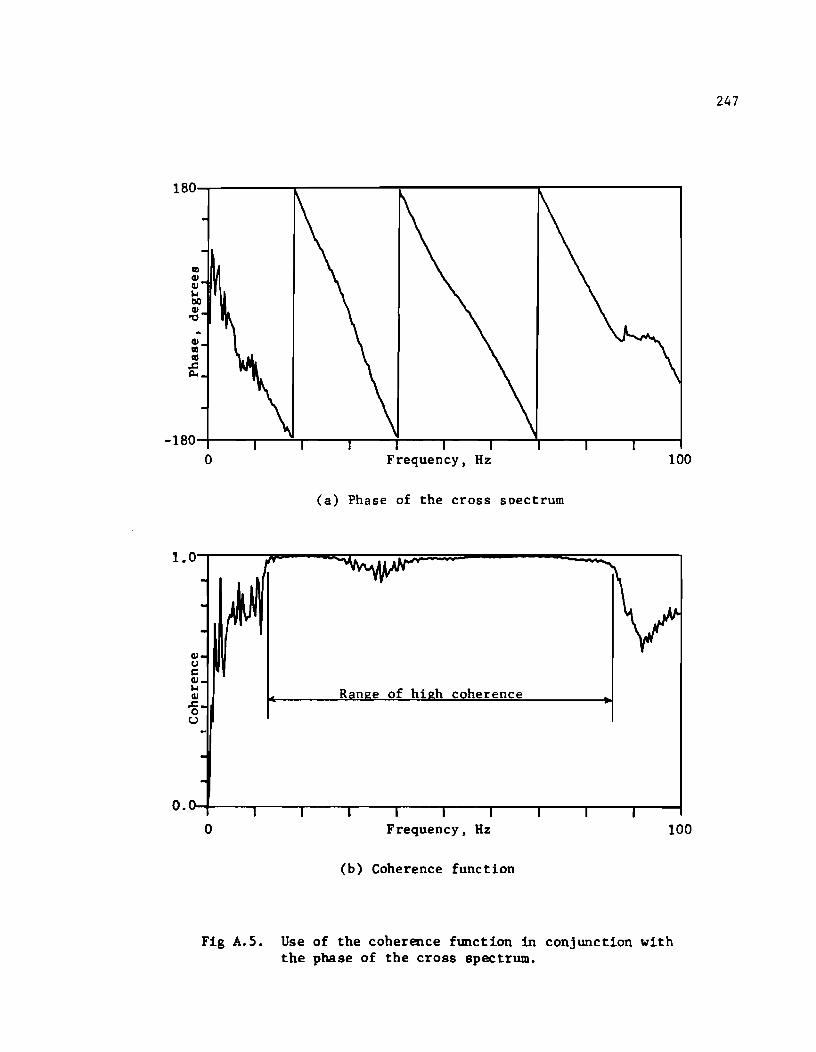
l80-r--------.---------~------------~------------_,
-180-r----r-~~--~r_--~--_,----,_--~----~--~--~
o Frequency, Hz 100
(a) Phase of the cross spectrum
O.v-~---r----~--~~--_r----~--_,----_r----T_--~----~
o Frequency, Hz 100
(b) Coherence function
Fig A.S. Use of the coherence function in conjunction with the phase of the cross spectrum.
247

248
+18 III CI) CI)
'"' 00 CI)
"'0 0 CI) III co if
-18 0 Frequency, Hz 20
(a) Original ("Displayed") phase plot.
+18~----------------------------------------------~
-18 III CI) CI)
'"' 00 CI)
"'0
CI) III co f
-54
-90~----~--~------------~----__ --~--__ ----~--~ o Frequency, Hz 200
(b) True ("Unraveled") phase plot.
Fig A.6. Comparison of "Displayed" and "Unraveled" phase plots.

249
apparent shifts result from slight variations in the phase and are not actual
phenomena.
Utilization of Computer Programs
The computer programs used to reduce data and plot results do not
contain complicated algorithms. The purpose of the programs is to perform a
large number of repetitive calculations which would require significantly
more time to perform by hand. The plot routines also feature the flexibility
to compare the influence of various parameters on the velocity profile.
Details of how each program functions and what data each requires are given
in Appendix B. For the most part, only the role of each program as it
relates to the analysis process is discussed in this section.
The first step is to reduce all of the available records (measurements)
using program PHAS. PHAS uses the phase information from the cross-spectrum
to calculate a travel time for each frequency that is given. The phase
difference, e, between the signals of the input and output geophones
represents the time lag or travel time, 6t, for an R-wave (of frequency f and
velocity VR
) to propagate over the distance between the two geophones. The
phase difference is 360 degrees for a travel time equal to the period of
wave, T. With T/360 as a proportionality factor, the relationship for travel
time is
T 6t • 360 0 8 (A.I)
Because the frequency is the inverse of the period, travel time can be
written as
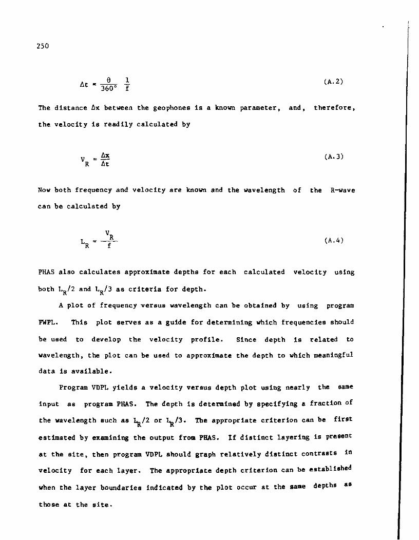
250
e 1 l1t = 360 0 f
(A.2)
The distance ~x between the geophones is a known parameter, and, therefore,
the velocity is readily calculated by
(A.3)
Now both frequency and velocity are known and the wavelength of the R-wave
can be calculated by
PHAS also calculates approximate depths for each calculated velocity using
both LR/2 and LR/3 as criteria for depth.
A plot of frequency versus wavelength can be obtained by using program
FWPL. This plot serves as a guide for determining which frequencies should
be used to develop the velocity profile. Since depth is related to
wavelength, the plot can be used to approximate the depth to which meaningful
data is available.
Program VDPL yields a velocity versus depth plot using nearly the same
input as program PHASe The depth 1s determined by specifying a fraction of
the wavelength such as ~/2 or ~/3. The appropriate criterion can be first
estimated by examining the output from PHASe If distinct layering is present
at the site, then program VDPL should graph relatively distinct contrasts in
velocity for each layer. The appropriate depth criterion can be established
when the layer boundaries indicated by the plot occur at the same depths as
those at the site.

251
In addition to VDPL, layering may also be depicted in a plot of
frequency versus velocity provided by program FVPL. Lines which separate
contrasting velocity layers and which pass through the origin will have a
slope of l/LR
• From the slope, wavelengths (and subsequently, depths) can be
calculated for each layer boundary.
Analysis of Results
Analysis of the results must coincide with the use of the programs and
plot routines in order to determine the velocity profile. The selection of
an appropriate depth factor for the plot programs relies on an analysis of
the calculated velocities and corresponding layering.
In addition, any apparent anomalies in the velocity profile should be
checked. The frequency and phase which yielded an unusually low or high
velocity should be traced back to the cross-spectrum from which they came.
The corresponding coherence function should be re-examined to verify the
quality of the measurement at that particular frequency. The phase plot
should also be rechecked to make sure regions which exhibit apparent phase
shifts (the effect of the lBO-degree limit) have been interpreted correctly.
Finally, the velocity profile may be refined by eliminating some of the
scatter associated with wavelengths not suitable for the spacing between
geophones for a particular aeasurement. A workable criterion was developed
in Chapter 4 and was given (Eq 4.5) aa
(A.S)

252
Wavelengths (or frequencies) which do not fall within the constraints of
Eq 4.5 can be screened out by checking the output from PHASe Inappropriate
data can be excluded from the final data arrays prior to using VOPL for the
final velocity profile.

I ".
,.
APPIRDIX B
OOMPUTD. PROGRAMS AND PLOT ROUTINES

I.:··'· i" , ~ ,

APPENDIX B
COMPUTER PROGRAMS AND PLOT ROUTINES
This appendix includes a listing of each computer program and plot
routine used in the reduction and analysis of cross-spectrum data. In
addition, a brief description of the capabilities, limitations, and input
requirements precedes each program. Sample input and output are included for
the reader~s benefit.
255
256
B • 1 • PROGRAM PHAS
Program PHAS is the foundation program for the reduction of
frequency-phase data. A major portion of PHAS also serves as a first state
in each of the plot routines. The input data file for program PHAS can be
readily modified to use with any of the plot programs.
Principal variables in PHAS are defined in the variable list of the
program listing. Input variables include: NREC, DATFIL, RECN, TRKN, Xl, X2,
BW, SOURCE, and the primary data arrays FR (frequency) and PH (phase). All
data can be input with free-field format with the exception of the
alphanumeric titles DATFIL and SOURCE. Input of a negative number for a
value of frequency terminates the input of (f,6) pairs and concludes the
input of data for that particular record. A sample input data file is shwn
in Fig B. L
Details on how to select values of frequency and phase are given in
Appendix A. The input phase (PU) is that value which was obtained directly
from the frequency-phase display. The computer program calculates the "true"
phase or "unravelled" phase by tracking the switch from -180 degrees to +180
degrees by means of the integer variable NP. The value of NP is initialized
as zero and is increased by 1 each time the l80-degree switch occurs. The
limits on the switch are quite liberal; if the present value of PH is greater
than 45 degrees and the previous value of PH was less than -90 degrees, the
program assumes that the -180 degrees to +180 degrees switch has occurred.
These limits provide minimal restraint if e is changing rapidly as a
function of frequency. However, input data should be checked to make sure
that erroneous switches cannot be interpreted from a particular sequence of
phase values.

PROGRA" PHAS(I~PUT,OUTPUT,TAPE1.1NPUT) C C THIs PAO&RAM USES PHASE INFORMATION FROM C THE C~OSS POWER SPECTRU" TO DEvELOP A C VELOCITY V8 DEPTH PROFILE C C***········.····_-**--*-*-*******-***-***·******-*···-.*-_ ...... * •... C VARIABLE LIST
C··········*_····*·····**···**·*···*··***·*·*·_*******-**.***.****-*-* C 8W RA"OWrOTM (RANGE OF FREQUENCIES) OF NEA8URENENT C CNVRT vALuE USED TO CONVERT R.wAVE vELOCITy TO I-WAVE VELOCITY C DATFIL TITLE FOR IDENTIFICATION 0' SINGLE DATA FILF. C DEL' FREQUENCy RFSOLUTION OF NEASURENENT C DELT T'"E RESOLuTION OF MEASUREMEN' C DELX DISTANCE 8ETWEEN GEOPHONES C OL2 DEPTH CALCULATED USING WAVELENGTH DIVIOEO Ay ~ C Ol3 DEpTH CALCULATE~ USING WAVELENGTH DlvIOEO BY 3 C FA(' FREQUENCV INPUT ARRAY C F.ACT NU~8ER 8v wHICH wAVELENGTH IS DlvIO!O TD OBTAIN OEPTH C ~P PARA"ETER US£D TO UNRAVEL FREQUENCy_pHASE PLOT C HREC ~'"8ER OF RECORDS TO 8E READ FOR A GtVEN RUN D' PROGRA" C PHe) PHASE INPUT ARRAY C PHAOJ ADJUSTED PHASE VALuE AFTER UNRAVELING C AECN IlfCORO NUMBER (FROM HPIj423A TAP!) TO IDENTIFY DATA C SOURCE TITLE FOR SOURCE USED TO MAKE MEASUREMENT C TITLE TITLE FOR FIGURE OF RESULTANT PLOT C TMLE~ TIME LENGTH OF "EASUREMENT C TRkN TRACk ~UM~ER CFRO" HP~A~lA ,APE) TO tDENTIFy OA'A C TT CALCULATED TRAVEL TIME OF WAVE C TTM CALCULATED TRAVEL TIME IN MtLLISECONDS C vEL CALCULATED YFL~CITV C WLl CALCULATED WAVELENGTH, WL( ) IS USED IN PLOT PAOGAA"S C~, ~JSTINCE FRO~ SOUACE TO FIRST (NEAR' 'EOP~ONE C ~2 DISTANCE FRO~ SOuRCE TO SECOND (FAA) GEnPHONE
c·.·*-···-·**··*·*·*·*········-····*_·····.*·.***-···**-*****.** .. *.*. INTEGER DATFIL(5),SOURCE(I.),RECN,TR~N OIMENSION FA(50),PH(50) READ (t, ) NAEC DO '16 tREC.l,~REC PlthT In
18~ FORMAT <-t_,lX) AEAO lAt,(O'T'IL(N),N.l,~) READ (1, ) R!CN,TRKN REAO Ct, ) .t,.l,B~ REID tAl,(SOUACE(N).N."t~)
1~1 FnRMAT (X,Al,.A.) l PZ FOA~AT CX,I3,_I.)
DELlf.XZ·xl OELF.B;,j/25".~ TMLEN.t.e/OELF DELT.TMLEN_I'.~.P/1824.P PAINT IA3,(DATFIL(N),N.1,S),'ECN,TAKN
SRI FOA~AT(X,lA"OATI FILEI,X,Al,.A4,lX",MTAPE AECORD NO •• , I Ia,IHc,ll,lH») 'RHo'T I'"'' Xl, Xi
1"4 F"AMAT (X'ltHGEOP"~NES LOCATED AT ,F.,a,aM FT AND "',2,IM 'T, 'ltttlT lplj,oEl.
1~5 FOAMAT C.,laHOI,TANCE BETWEEN GEOPMONES. 'F'~I,JH FT) PAINT IP',(50URC£(~),N.t,1~)
till. 'ORMAT (X,1MSOuACh,X,A3,cua, PAINT l,7,ft.,DELF
251

258
1~7 FORHAT C1,I~H8ANOWIDTHI,FA.l,3H HZ,8x,IIHA£SOLUTIONI,Fa. G,3H HZ) PAINT 10e,TMLEN,DELT
lae FOAMAT (X,11HTI~ELF.NGTM.,F7.2,4H S£C,7X,IIH.fSCLUTIo~.,Fe.4, I 51'! MSEC)
10.1 I~~ AEAO CI, ) FACIOJ,PHCIOJ
IFCFACIO).LT,I.B) Gn Tn 110 to_IO+1 GO TO 10~
1111l I"F-IO-I PAINT III
III FORHAT CIl2X,~HFREQtlENCY,"l(,5HPHAS!,]X,lftHTAAVEL vnocn't', 1 2X,13HWAVELENGTH,ft X,5HDEPTH)
PAhlT 112 III FORMAT ClGX'4HTJ~E,2bX,3HL/2,5X,3HL/])
P"INT 113 113 FOA~,T (QX,4H(HZ1,5X,16H(OEGAEES) (HS[C),lX,SHeFPS), I 7X,4MCFT1,b X,GHCFT),4X,4HCFT)J
PAINT NP.", 00 115 IO_I,IOF IFCPHCIO).GT.45.A.AND.PHCIO.I).LT •• ~0.~) NP.NP+I /lfIllP-NP PHAnJ_CANP.CPHClnl/]60.0»a]ft0.a TTaPHAnJ/]bB.Q/'''(I") TTM_TTaU01!!.9 VEL-OELX/TT wLlavEL/FPCIO) DLla1olL1 / 2.lI! DL3a"LtI].A PAINT 114,FRCIO),PHACJ ,TTM,VEL,WLI,OL2,DL]
114 FORMAT ClX'F8.J,3X'F7.2'F'.3'FO.l,4X'F7~3,'-X'2C2X,'b.3» 11 5 CONTI~UE 11ft CONTINuE
END
'I

1 ------- NREC FIG. B.3. 51~PLE PlnT Fnk PROGPA~ VDPL
." 1smA -----_ DLIM, VLIM * TInE (for Plot)*7 1 • ~, , 3 CNVRT, FRACT *
SA MPl E DATFlL " , H RECN, TRKN '5, HJ, 321P, Xl, X2, BW
yf)EAl H,"'MER -SOURCE 21'4,-58.9 ?'5'."~."" 3~,.qA.1e tI~,.'~2.el "",-15Cl!.e1 65, tf .. a.~l 10~', fiG. 4t1 tlt;,.1S.12 t7C1J,-t2q.,~ ?tr;,US.3t ?J-;, ltlj~ 12 ~5n,!;t1§,6~ 13q,.l2.15 ~~",.154.~e 450,'''.1 13 54",.t34.31 ""''',144.26 fU:'A,.U~2.Jt q6l1J,,,~.tt
tlaa,·2.!i1.l 13,,1',. t 66. ]«;
11.11.4",." .~1J1 1'5\"1",,·«;.,.20 1''''''',118.IA t8.-0,-,'4.Q7 1 «;AtII,'IfI.22 2D1c-~,.IP.~ 51.1
FR( ), PH( )
.. 1,0 .~------- Counter used to terminate input
for particular data file. * Only used for plot programs.
Fig B.I. Sample input data file.
259

260
The reduced data and calculations are output in a table which includes
frequency, "true" phase, and the travel time, velocity, and wavelength of the
wave associated with each particular frequency. Values of depth based on
~/2 and LR/3 are also listed. Each new record yields a summary table, such
as Table B.l., beginning on a new page. There is no limit to the number of
records (NREC) which can be reduced in a single run of PHAS.

261
OAT. rlLEI SAMPLE UPE RECORD NO.1 ~on
GEOPHONES LOCATED AT 5.~0 'T AND 11'.00 'T OISTANCE BET~EE~ GEOPHONES, 5.13 'T SnURCEI IDE'L """'HER 8AND~IDT"'1 320R.8A "'Z ~ESOLljTlONI 12.511Cl1 HZ lI"'EL£HGTH, • 1iI8 nc NESOLUTION • • .,181 "'SEC
FREQUENCY PHASE TRAVEL VELOCITY WAVELENGTH DEPTH T UtE L./Z L/l
(HZ) (DEGAEESl (MSEC' (,PSl eFT, (FT) tF J)
2111."0'" 58.1& 8.ltlb4 b211)." :11 • B!a(t lS.lildl H1.31JJ 25.kl ilJlI 71.71 8.1n &PI.S iO,IIQ1", 12,Z~" e. 111 3il,U" '8.t8 8,35~ 5"8,& l',~bA "q8~ &,053 4ft1."'01i! 122. lit] 1'.474 5Qe,li1 1",75A 7.375 4.~17 lI!h:l.I,e 150. Al 8.334 &0M.~ 11.'''' t).~"':A la.oJ'lL' f:I5 •• I&!W 1 '5.ll 8.13 Q 5",& ",22r; 4.e.12 3. ·)7~
I !'1-', "'''II 2'5."" 8.1'7 bUt,A blUR 3.050 2."3\ 115. "Gte l'5.U 8.110 b15.0 0.1556 2.2113 1,51I'J 170.lee 18'.e., 8.a00 bl5.0 3.a7" 1,81A t. 2 2«; 2tS.0111111 &H4.b' 7.813 b4".1If i.'7? 1.488 ,-.qj) i3'5.IiIIII &84.l8 7.103 ?"",I 2.'7q t.48' ."" is't.IUS 5'4.]5 0,004 757.1 1,~2' 1.514 1.'Ol n
31"',1"" 1Ql.25 0.248 81.911.3 2.425 1.211 .80)00 3''',18a no. 'b 0.232 8~'.] 2.057 1.02' .O8#'} 45"."'" "'." b.112 eU.l 1.8;1" ,'I;} • tI~i' 54 lot ,111111 1214.37 b,241 a011i,4 I.08i! .7al .C4qu DIU'.''', 12'5." S.'" 8]1,5 1.38' .b'5 .&103 8~"."1' to".ll 5.5&4 8'8.7 1.121 .Sb2 .37 /J
QbU."I. 1111.8' 4.'59 Utl,I 1."52 .5l6 .151 tl~".".1 1882.541 4.552 1II'a.4 .q'Q ,4" .113 t l'Ut, iii I & 1'00.3' '.282 Sl'''.1 .'11ii .'158 .10~ lGRu.8el 2112.'7 4.U2 11'2.0 .85~ .426 .iea t 5"]1.'8' 2251.'0 G ,180 1100.2 .7', .3" .Cbb 10104".1111 2481." '.1714 1 ,,'.fa ,149 .375 ,l5\~ 18 IHt. IIJII ZfllU.97 4.1'5' 1202.2 .bU .111 .12:J \'\I~,all! 282q.18 G.137 12P.8.b .ft3" .318 ,liZ 2~,n". UII 2'aq,54 '1.152 12141,2 .6"2 .381 .llt
Table B.l. Sample output from program PHAS.
262
B.2 PROGRAM FWPL
Program FWPL uses the reduced frequency and phase data to plot frequency
versus wavelength. There is no limit to the number of records which can be
stacked together for a single plot. However, each record is plotted with the
same symbol. The data input is nearly identical to the one used for PHAS.
Three new variables (TITLE, FLIM, and WLIM) are required and are input
immediately after NREC, prior to reading the first record. The alphanumeric
variable TITLE is an overall title which serves as a caption for the plot.
Variables FLIM and WLIM are used to establish the limits of the plot.
Values of frequency are scaled to a 5-inch horizontal axis while values
of wavelength are scaled to a 7-inch vertical axis. In order to avoid the
irregular bounds set up by the plot commands, a sorting routine is used to
establish rational bounds and to screen out data outside these bounds. Both
variables, wavelength and frequency, have lower bounds of zero. The maximum
value of frequency is not fixed and must be input as var1able FLIM.
Similarly, the maximum value of wavelength must be input as WLIM. The
scale(s) for the plot are then determined as I inch - FLIM/5 and
linch = WLIM/7. Appropriate selection of FLIM and WLIM will yield a plot
which can be conveniently used with an eng1neerOs scale. A sample plot for
program FWPL is shown in Fig B.2.

PROGRA~ FWPL(INPUT,OUTPUT,TAPEI.INPUT,PLOT~'
C C THIs PROGRA~ USES PHASE INFOR"ATION FROM C THE CROSS POWER SPECTRUM TO DEvEL~P A C FREQUE~CY VS WAVELENGTH PLOT C C ••••••• •••••••••••••••••••••••••••••••••••••••••••••• •••••••••••••••• C INITIALIZES ppnGRA~ TO AEOUCE AND PLOT NREC NUM~ER OF C RECOROS STACKED TOGETHER C·.·················· .. · ... ··························· ............... . INTEGER 'ITLE(ft),DATFJL(~),SOURCE(IR),AECN,TRKN
DI"ENSION FR(S~),PH(S~),WL(SP),PFR(SA),pWL(Sm) READ (I, ) HREC READ 1~~,(TITLE(N),N.I,ft)
lei FORMAT (SAtP) ~EAD (1, ) FLI~,wLIM CALL PLOTS (0.~,~.~,SHPLOTR) CALL PLOT (1.8,2.0,-]) DO 12m IREC-I,NAEC
c·.···················.·.·.··························· ............... . C PEADS DAU FOR C"P~ENT RECORD C •••• •••••••••••••••• •••••• ••••••••• •• ••••••• •• ••••••• •••••••••••••••• REAO 191,(OATFIL(N),N.I,S)
~EAn (t, ) RECN,TAKN READ (1, ) XI,.2,8w PEAO Ipl,(SOU~CE(N).N_I,t0)
IPI FOAMAT (.,A],GAI) 1-2 FON"AT (X,A3,.AG)
DELX.X2- Xt DELF.eW/2Sit.B TMLEN·l.e/DELF DELT.T~LE~·10ep.a/leiQ.9 PRINT IAl,(DATFIL(N),~.l,S),PECN,TRKN
103 FnRMAT(X,IAHOATA FILEI,X,A3,4AG,]X,17HTAPE RECORD Nn~1 , 1 I2,lH(,Il,IH»
PRINT 184,Xl,1(i 1~4 FOA~AT (X,21HGEOPHONES LnCATEO AT .Fit~2,~H FT AND ,Fit.2,3H 'T'
PRINT US,OELX lAS FDR~AT (X,leHOIsTANCE BETwEEN GEOPHONES I ,'6.2,]H FT)
PAINT 1~o,(SOURCE(N),Nal,13) IA6 ,OP"AT (X,7HSOU~CF-I,1(,A3,.A4)
PAINT lA7,a.,D~LF lA1 FORMAT (X,leH~ANnwIDTHI,F~.2,]H HZ,8x,IIHAESOLUTIONI,Fe~.,lH HZ'
PAI~T lA~,TMLEN,~ELT lift FOAMAT (X,1IHTIMEI.ENGTHI,F1.2,IM SF.C,1X,11HAESOLUTIONI,'8.G,
1 I§H ",SEC) PRINT 1°·1
II. REAn (1, ) F~(lo).PH(IO' I'('R(IO).LT.~.~) GO TO ll~ IOaIO.l GO TO h.
ll~ 10F.IO-l c· ••• •••••••••••••••• •• ••••••••••••••••••••••••••••••• •••••••••••••••• C CALCULATES FREDUENCY, VF.L~CITY, AND WAVELENGTH INFORMATION
c·····················.·.····························· ............... . NPa~
00 1 tl I Oat, IOF IF(PH(IO).r.T.45 ••• ANO.PH(IO-l).LT.-QS.0) NPaNP.t RNPaNP PHADJa(R~p-(PH(IO)/lb0.a».36P.m
263

264
TTaP~.OJ/3~e.e/FA(IO) vELaOELXITT WLClo)avEL/FRCIO)
1 t I CO~Tt NUE c********************************************************************* C SORTS fREQUF.~CY ANO .AVELENGTH ARRAVS TO PREPARE 'OR C DESIRED PLOT 'ROM CURRENT RECORD C*********************************************************************
PRI'lT 112 pRl~T
112 FORMAT ()X,17HDAT' FOR PL"TTI~G) DO 113 loal, 10' IFCWL(IOl.LT.WLIM) GO TO II'
113 CONTINUE II' IOB.IO
00 It S lOa t , tOll' I,C'RCIO).GT.FLIH) r.O TQ 116
tiS COHTINU! I/)atO'+1
In Il)taIO-l 10Pal DO 118 IoatOB,tOE P'RU np l.FR tIO) PIIILCIOP)a.UIO) PRIHT tt1'IOP,P'A(IOP),PWL(IOP)
II? fORMAT (2X,I~,2(5~,Fl~.2» IOPaIOP·1
It 8 CONT lHuE c********************************************************************* C SETS UP PAAAHET[RS AND EXECUTES PLOT 'OR CURRENT R[CORD C*********************************************************************
"IIITSatOp .. t ICC¥CLhl PFR(NPTS+l)·IlI.~
FINCa'LUVS.0 P'RCNPTS+Z).FINC PWLCNPTS.t).WLIH WtlfCa.WLJ",I1.1 PWL(HPTS+2).WI~C JF CIAEC.OT.l) 00 TO llq CALL svH~Ol ( •• S,.I:~ •• ll,TITlE.e.e.S~) CALL 'XI' (0.~,7.~,!~H'REQUENCY, ~l,ll,5 •• ,R~~.'~P,'INC) CALL AXIS (~!e,p.~.tIHwAVELENOTH, 'T.l •• 7.~.,~.',WLIM,WINC)
l1q CALL LINE (PfR.PwL,NPTS,kCYCLE,-t,3) C*******.***.*.****** ••• *****.*.*********-***.******-***.****.* •• ***** C R[SETI fOR N[W R(CnRD C*****************.*****.**********************************-*_._****-*
PRINT ., .. CONThll.IE
C*************************.************************.*·** •••• *********. e CLOSES PLOT ,~O TERMI"ATES 'InCR,,,, C****.*-*************-*************.·************-.**-*.* •• ** •• _* •• *.*
CALL PLOT (8.S,~.g ••• ,) END

§J.oo FREQUENCY,
40.00 80.00 HZ -10 1
120. 00 160. 00 200.00 .~----------~----------~----------~----------~--------~ o
0 0
· If)
0 0
· 0 -1-0 (LO
· If) .-:::c l-t!> Zo Wo ..J. W O
>N
a: ~
0 0
• If) N
o o · o
(r)
o o
• If) (r)
+ + ++ ++
+ ..... +
+
+
+
+
+
+
+ + + + + + + +
Frequency
11.11111 n.IIB ]I.II~
111.8" ~'.II" o,.dill
'''".lIfe U5.1I" 1'711.110 1I5.IUI US.IJ'" Z~B.lli nl.lI.., ]qlll.1I9
a5"."" 5alll."" 611111 • .,0 U".II~ .,,.1."0
11I'1t.1!1II UIIII."" lalll.IfB 15"1.1111 16".1" 18"11.10 ' .. , ..... ZliUltJ.1f1ll
Wavelength
]I.u Z4./a ,q • .,o 1".75 II."" q.ll ,.. 1\11
".5' 3.e.e l.qe l.ql! 3.U 1.43 2.~. I.e~ I.III! 1.31' t.ll 1."'5 '.015
.qZ
.85
.80
.'7~
.6'7
.611
."111
Fig B.2. Sample plot for program FWPL.
265
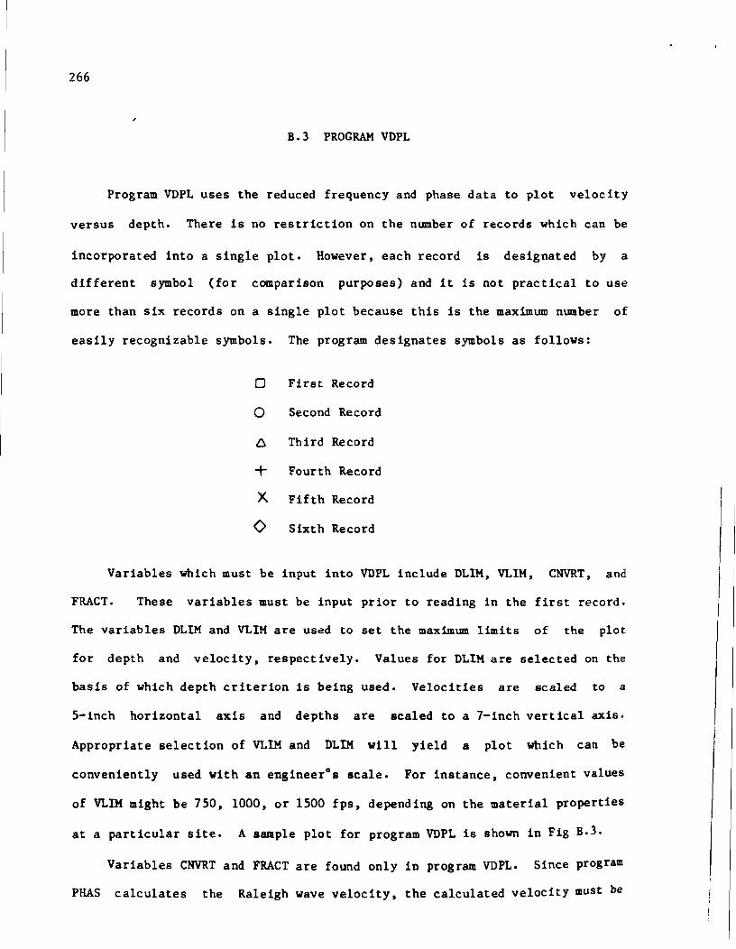
266
B.3 PROGRAM VDPL
Program VDPL uses the reduced frequency and phase data to plot velocity
versus depth. There is no restriction on the number of records which can be
incorporated into a single plot. However, each record is designated by a
different symbol (for comparison purposes) and it is not practical to use
more than six records on a single plot because this is the maximum number of
easily recognizable symbols. The program designates symbols as follows:
0 First Record
0 Second Record
~ Third Record
+ Fourth Record
X Fifth Record
0 Sixth Record
Variables which must be input into VDPL include DLIM, VLIM, CNVRT, and
FRACT. These variables must be input prior to reading in the first record.
The variables DLIM and VLIM are used to set the maximum limits of the plot
for depth and velocity, respectively. Values for DLIM are selected on the
basis of which depth criterion is being used. Velocities are scaled to a
5-inch horizontal axis and depths are scaled to a 7-inch vertical axis.
Appropriate selection of VLlM and DLlM will yield a plot which can be
conveniently used with an engineerOs scale. For instance, convenient values
of VLlM might be 750, 1000, or 1500 fps, depending on the material properties
at a particular site. A sample plot for program VDPL is shown in Fig B.3.
Variables CNVRT and FRACT are found only in program VDPL. Since program
PHAS calculates the Raleigh wave velocity, the calculated velocity must be

PROGRA" VOPL r I NPIiT , OIlTPIIT, TAPE I. I "'PUT, PLOTIn C C THIS PROGRAM USES PHASE I~FORMATInN FROM C THE CRnss POWER SPECTRUM TO DEVELOP A C vELOCITY va DEpTH PLOT C DEPT~ DETERMINED AS FRACTION OF wAvELEIIIGTW C C·*·.· .. ····*··*··*···.·.·.*·························· ............... . C INITIALIZES PROGRA~ TO REDUCE A"'D PLOT ~AEC Nu-SEA 0' C RECORDS STACkED T~GETHER
C· ...... · ... *.·· .. *.· ....... * .. * .. * .. * ......... * ..... · ... * .. * ........ . INTEGER TITLE(8),DATFtL(5),SOUqCE(I~),~ECN,TA~N ~IMENaI~N FR(5R),PHC5e),VELCSe),wLC5A),PVELCS~),pwFC5e) READ (1, ) NREC READ le0,(TITLECN),N.l,8)
IAA FORMAT CaAIA) RUO Ct, ) DLI",VLI~ READ (1, ) CNVRT,FRACT CALL PLOTS (e.A,~.0,5HPLOTR' CALL PLOT Cl.8,2. Q ,-])
ILETT." DO 12a IREC-I,NREC
C· ...... ·* ... ····· .. · .. ·.· .. *· .. ··.· .. *.··.·· .. ·.·.*·· ... * ........... . C READS DATA FOR CURRENT RECORD c·.···*.·*.·*······*··*·.* .. · .... ··· .. *.··.·· .. ·.····· ............. * .. READ IMI,(DATFYLCN),"'.l,S)
REA~ (I, ) REC~,TRk~ REAO (I, ) Xl,X~,RW READ tA~,(S~URCE(N),N.I,le)
101 FOR~AT CX,Al,4A4) IAZ FORMAT (X,A3,~A4'
OELhXZ.X I OELF.8"1Z56.~ T"LEN_I.A/OELF oELT.T"LEH·t~R0.P/te24.e PRI~T t81,(OATFILCN),N-I,S),A£CN,TRkN
tA3 FOR"AT(x,t0HOATA FILEI,X,A3,aA4,3x,17HTAP£ REeoR~ "'O~I , t IZ,IH(,It,IH»
PRINT ,19I1,xl,xZ IRII FOR"AT CX,2IHGEOPHONES LOCATED AT ,F6.2,8H 'T ANO ,F6~2,3H 'T)
PAINT I"S,DELlC IPS '~A"AT CX'Z8~~tSTANCE 8!TwEEN GEOPHONES I ,F •• 2,3H FT)
PRINT IAo,CSOURC£(~,,"'-I,tP) tilt. FOIU.AT (X,7HSOIJACEI,x,Al,eU4)
PRINT lA7,9~,DELF lP7 FORMAT CX,IMH~ANOWInTHI,FA.2,lH HZ,8X,11HRfSOLUTIONI,'4.4,3H HZ)
PAINT t0a.TMLEN.nELT IRa FOAMAT (x,IIHTI"FLENGTNI,F7.2,4H SEC.7X,1IHRfSOLUTlnN.,F8.4,
I 5H "'SEC) PAINT lOa.
IRq READ CI. ) FR(IO),PH(IO) IF(FR(ID).LT.A.A) GO Tn lie In.Io.l GO TO In
II" IOF-IO.I c········.···········.·· .. *.· .... ·.· .............•.. * ••••••••••••••••• C CALCULATES 'R~gUENCY, VELOCITY, AND NAVEL!"';TH I",'ORMATynN c·.··· .. * •• •••••••• •••••••••••••••••• ** •• * ••• * ••• * •••• * •••••••••••• *.*
IIIP.~
DO tit IO_t,IOF
267
268
t'(PHCIO).GT.G5.~.'ND.PHcrO.l).LT •• 9~.') NPaNP., A-.PaNP PW'DJ-(~NP.(PH(ID)/36B.e)'*3b~.e TT-PH,oJ/36e.~/FR(IO) VEL( IO).OELlC/TT WLCIO).VEL(IO)/FACIO)
111 CONTI NUE C*******************************.*.**** •••• ** •• ·.* •••••••••••••••••• *. C SOATS VELOCITY 'NO WAvELENGTH A~RAY TO PREP'~E FO~ OESIRED C PLOT FRO" CURAENT RECORD C·.*********.** •• ** •• **** •• ******************.****.*.****** •••• **.*.*.
WLI .... FAACT*DLI" PRINT 112 P~INT
liZ FOA"AT Clx,11HOATA FOR PLOTTING) 00 113 IO-t,tOF IFC-LCtol.LT.WLIH.AND.VELCIO).LT.VL!M) ;0 TO 114
1 13 CO~TINUE 114 10".t O
DO tIS I08roe'tOF IFCVELCIO).GT.vLIM) Gn TO lt6
11 5 Co.,T I ",UE 10-10'+1
116 10Ea10-l 10Pat DO 118 to-IDA,IOE PYELCIOP).vEL(IO)/CNVAT P~FCtOP)-WL(IO)/'A'CT PAI~T tl1,IOP,PYELCIOP),PWFCIDP)
111 FOA~AT ClX,t4,2(5X,FIR.Z» 10P·IOP+1
118 CONTINUE tOPhlnp-l
C**************.**************************************.************_** C SETS liP PAifAwET!.'R! ''''[\ EICECUTES "LOT FOR CUJUtE"T .ECORD C********-**_********.**.**** •• ****.** •• *.*********.*****.************
NPTSaIOPT KCYCLEat PvEL("'PTS+l'-I.~ VINC.VL! Mi5." PvELCNPTS+2)·vINC PwF(NPTS+t).OLIM DINC •• OLIH/7.ra pwFCNPTS+Z)-DINC 1'(1AEC.GT.l) GO T~ 119 CALL SYMBOL ( •• ~,·1.~ •• lZ.TITLE".R.~0) CALL AXtS (~."7.~.13HY!LOCTTY, FPS'13,~~ •• e:A •• :e,VINC) CALL 'ICIS C~.e,~.A,~~O(PTH, FT,.,7 •••••• R,OLIM,DTNC)
l\q CALL LINE (PvEL._WF,NPTS,kCVCLE,el,IL£TT' C***********.****************************.**************************** C RESETS FOR NEW ~ECO~O
C*.***·.* •• *.·····*****.**************************.*****************.* ILEThILETT+t PRINT
tI~ CONTINUE C*·****·*****************************.******************************** C CLOSES PLOT AND TERMINATES PAOCA,M C***********.*******************.**************.************.*********
CALL 'LOT (e.5,~.R, ••• ) END

269
Fig B.3. Sample plot for program VDPL.

270
converted to a shear wave velocity. The conversion factor CNVRT is a
function of Poisson's ratio and is given by
The value of CNVRT will always be less than 1.0. Additionally, the depth z
which is associated with a particular velocity is defined by a fraction of
the wavelength where
z - L /FRACT R
The value of FRACT is always greater than or equal to 1.0. When FRACT = 1.0,
the program provides a velocity versus wavelength plot.

271
B.4 PROGRAM FVPL
Program FVPL uses the reduced frequency and phase data to plot frequency
versus velocity. The velocity that is plotted is the calculated Rayleigh
wave velocity. There is no limit to the number of records which can be used
for a single plot. However, it is not practical to use more than six
records, since each record is designated by a different symbol as in program
VDPL. Values for FLIM and VLIM must be input to establish plot limits.
Frequencies are scaled to a 7-inch vertical axis while velocities are scaled
to a 5-inch horizontal axis.
Fig B.4.
A sample plot for program FVPL is shown in

272
P.OQRAM FVPL(JNPUT.OUTPUT.TAPEl.I~PUT.PLOTR) C C THIs PROGRlM USES PHASE INFOA~lTION FRO~
C THE CROSS POwER SPECTRUM TO DEVELOP A C 'REQUENCY va vELOCIT' PLOT C C***********.**··*****.*.*·*··.**··*.*·*.·**····**·***********.**** ••• C r~lTIAL1ZU PROGRA'" TO R!DIJCE A"'D PLOT HAEC HUM8ER 0' C RECORDs STAC~EO TOGETHER C****·**·************************* •• *.***** •• *.*.**.***.* •• ********.**
INTEGER TITLECAJ.OATFILCS1,SOUACECIP1.RECN,TRMN DIMENSION 'R(50l,PM(58),vEL(5~1.wL('I).pvEL(5R).P'RC5') ilEAl) (I, ) HREe READ t R0,(TITLE(N),"al,8)
l~A FORMAT (8l1~) READ (1, ) ,LIM,VLI" ClL\. PLOTS (0.~,~.0.5HPLOTR)
CALL PLOT Cl.~.2.S,·3' ILETT." 00 t2e tREe-I,NAEC
C·.·.·.***.*.***.**.**.***********.*******************.*****.** •••• *** C RElDS DATA FOR CURRENT RECORD C***·*.*·**·*·************ •• ·***.**.** •• **.**.*******.**************.*
RElO lAl,CDlT'ILCN"Nat,S) READ CI, ) RfCN,TRKN RElD (I, ) WI,.2,BW READ 102 ,(SOURCE(N),Nat,le)
lMI FORMAT (X,j).4l4) 1~2 FDRHAT (!C,Al,qA4)
Of\.X-X2.Xt DELFaeW/256.0 TMLENal.e/OElF OELTaTMLEN*IAIR.~/t024.8 PAtNT l~),toAT'IL(~).~al.s),AEC~,TAMN
I~l FOR~lT (X,19HOlTl FILE:,X,Al.4A4.1X.t7HTAPE ArCORD HO ••• I 12.t H(,II,IH» PRINT 1flll,H, ,,2
1~4 'OA~AT (X'2IMG[OPMONES LOCATED AT ,' •• 2,~H 'T AND .".2,3H 'T) P!lINT I"S,OEl.t
IPS FORMlT (X'l~HOtSTANCE RETwEEN GEOPHONES. ,F6.i,3M ,T) PAINT 11I~,(SnUAC£(N),Nal,t~)
lBo FORMAT (l1,7HSOIIRCE •••• A3,ctU) PRINT lP7,~w,D!L'
IA7 ,nRMlT (.,1~"~lNDWIDTHI#F4.2.JH Hl,8 •• ltHAESO\.UTIONI"e;I,JH HZ) -RtNT t.8 ,TMLEN,DELT
1~8 FORMAT (X.JI"TIM!LENGTWI,F7.2,4H SEC,J~,11HR!SOLUTr~N.,F8.4, I 5H MSEC) PRtNT lOa,
l~' .rAO (I, ) FA(IO),PH(tO) 1'('''(tO).LT.~.A) CO TO lt~ IOaIO+t GO TO ,"'.
1111 10FaIO-l C**.* •••••••••• * •• *.*.***.************.**********.**********.********* C CALCULATES ,R[QUENCY. VELOCITY, AND WAVELfN;TM tNFOR"ATt"N c*******·***.***************·***.*******.*******************.*.******.
IliP., Of! 111 10.1,10' t'(PH(IO'.G'.'5.~.lND.PM(IO.1).LT •• "." NPaNP+l .NPaNP
I I I

P~AOJ-CR~P-CPH(10)/]h~.I"*3hl.' TT_PHAOJ/1~Q.I/FRCI0)
vEL (10) -OEUITT WLCIO).vELCIO)/FRCIO)
til CONTIloIlIE C-*_.· •• -.·_----·-·.· •• ·_ •• -·._.-._. __ .·_ •• -· •• • •• ··--_. __ •• _ ••••• _ •• -C SORTS VELOCITY A~D FMEOUE~CV ARRAv TO PREPARE FnR DESIRfO C PLOT FROM CURR!NT RECOAD C-••• • •• _.·_·_-···*·**.*_._--._*-.***-***.***.*·_·**·-*.* •••••• * ••••• -
PRI~T III PR NT
liZ 'ORMAT C3X,17HOATA FOR PLOTTING) DO 113 IU-I,IOF I,CVELCIO\.LT.VLIM, Gn TO 114
113 cONTINUE 114 1°9-10
00 II~ 10-IOB'IOF I'C'A(IO'.GT.'LI~.OR:V£LCIO).GT.VLIM) roo TO 116
115 CONTINUE 10-I Of +1
116 IOE-IO-I lOP-I 00 lie 10-IOB,IOE pVELCIOP)-VELCIOl PFRCIOP).FRCIO) PRINT 117,IOP,PVF.LCIOP),P'RCIOP)
117 FORMAT CZX,I4,2(5X,'IY.2» 10P-YOP+I
118 CONTINUE 10PT-IOP-I
C·_··-···*····--··_··._-*·· __ ··.-_··.····-.·-·.-.····· ••• __ ._ •• _ •••••• C SETS UP PARAMETEAS AND EXECUTES PLOT 'OR CURRENT RfCORO C·*.*-**·***-*··.** ••• - ••••• *.** •• * •••••• * •• * •• *.* ••• • ••• * •• *.**.* ••••
NPU-IOPT KCYCLEat PvELCNPTS+I)-~.~ v I NC .vU" 15." pvELCNPTS+2'·VINC P'RCNPU+t he.I 'JNC.FLII4/7.~ P'RCNpTS+Z)·'IHC I'CtREC.GT.2) Go TO II~ CALL SYM80L C •• 5,·1.5,.12,TtTLE,a.~,8~) CALL AXIS C~.9,'.~,13HVELOCITY, FP!,.tl,~.~,r;A,.;~,VINC' CALL AXIS CA._,A.e.11",RERU!NCV, "l,ll,7 ••••••• , •••• ,~NC)
11q CALL LINE (PvEL,pFR,NPT!,KCVCLE,.I.ILETT) C-*.*._*_ ••• *.*.** •• *.-*** •••• * ••• * ••• *** ••• * •• ·.*.*.·* ••••• *.* •••• * •• C Rt!ET! FOR NfW R!CORO C.* ••• *.** ••••••••• * •• - •• * •• _ ••••• ** •• *.* ••• * •• -_* ••• ·* ••••••• *.* •• - ••
ILETTaILETT+I PAttn
1211 CONTINUE C.*_.***-** •• _***·.* •• * •••••••• *-.** •• ** •••• * ••• * •• *.* •••• * •• * •• * ••• *. C CLOSES PLOT ~~n T£RMINATES PROQ.A" C*.*.·*.· ••••• ·**· •••• *._ •••••••••••••••• * ••• _ •••••••••••••••••• ** ••••
CALL PLOT (~.s,a.I,.qq) END
273

274
0 0
• 0 -N
f!J
0 0 f!J
• c VelocitI FreguencI CD I!J - 621.e5 2"'.0" 61".11101 25 .Illt ,.a.'''' 3" • .,-,
0 S"I!I.U 1I~.~\ot
0 5' •• "0 "I.I!'I" I!J • "".fu' .,5.".,
0 .I!'.'~ 1"~."0 In olS.lIt!.) tls.nt4 I!J - U5.90 "".IttY - U".rete it'S.IH!I I!J 0 701d.BS 235.0'" -0 n7 0 1J l5.'. "if MO 1'111.21 3]",.o~ I!J · 1U12 0 32 ]'111."" 0 IHIII.n 4ch'. ~irS NN 11I'!"'.4! 'SIUI.i1I9 :c- !ll.S" 604"'.30
•• ,. ?If 8"fI. "lit I!J .. I lf li.ffl1l CJ"".iillil
>- Ul~".45 11el!l.~~
W O 11·"."~ 13~~ • .,1tI ZO U CJ 2.U l43Ao~ra I!J We 11".11 115'-10.1918 ::JO) 11" .{,I(I 1".h'!l.0tlJ
0 12'2.24 18"" • "lit UJ
1118.57 "if0. ae I!J a: lID1 G.ilit l"",9.I!III
I.L.O C •
0 I!J CD
I!I
I!J 0 I!J 0
• I!J 0
'" I!J I!JI!I
I!J I!I
0 C9
0 & • 91.00 30.00 60.00 80.00 120.00 150.00
VELOCI Tl, FPS _10 1
Fig B.4. Sample plot for program FVPL.

J. Scott
16, 1956.
~i~y ~s ~rn
After graduating
THE AUTHORS
in Lancaster, Pennsylvania,
from Elizabethtown Area
on
High
October
School,
Elizabethtown, Pennsylvania, in 1974, he entered Drexel University in
Philidelphia. He received the degree of Bachelor of Science in Civil
Engineering from Drexel University in June 1979. In Sepetember 1979, he
entered The Graduate School of The University of Texas at Austin.
Kenneth H. Stokoe, II joined the faculty of the College of Engineering
at The University of Texas at Austin in 1973. He is presently an Associate
Professor of Civil Engineering and is actively involved
with several on-going research projects. He has been
working in the areas of in situ seismic measurement,
laboratory measurement of dynamic Boil properties, and
the relationship between field and laboratory dynamic
measurements for the past fifteen years. He was instrumental in developing
the in situ crosshole seismic method for shear wave velocity and shear
modulus measurements to the method that is presently used by most
geotechnical engineering firms.
In addition to his teaching and research activities, Dr. Stokoe has
served as a consultant to federal, state and private organizations in
the areas of Boil dynamics and geophysics. He is currently serving as a
275

276
consultant to the Civil Engineering Division and the Earthquake Hazards
Mitigation Program of the National Science Foundation.
w. Ronald Hudson is a Professor of Civil Engineering at The University
of Texas at Austin. He has a wide variety of experience as a research
engineer with the State Department of Highways and
Public Transportation and the Center for Transportation
Research at The University of Texas at Austin and was
Assistant Chief of the Rigid Pavement Research Branch
of the AASHO Road Test. He is the author of numerous
publications and was the receipient of the ASCE J. James R. Croes Medal. He
is presently concerned with research in the areas of (1) design of pavement
management systems, (2) measurement of pavement roughness and performance,
(3) rigid pavement slab analysis and design, and (4) low volume roads.
A. H. Meyer is a Senior Lecturer in the Department of Civil Engineering
at The University of Texas at Austin. He serves as an investigator on
several continuing projects through the Center for
Transportation Research. Before c~ing to The
University of Texas in 1980, he was with the Civil
Engineering ~epartment and the Texas Transportation
Institute at Texas A & M University. His area of
specialization is in pavements (construction, evaluation, and maintenance)
and pavement materials (portland cement concrete, rapid setting cements, and
polymer concrete).
In addition to his teaching and research duties, Dr. Heyer is active in
several professional and technical societies including the Texas Society of
Professional Engineers, the American Society of Civil Engineers and the J ,

277
Transportation Research Board. He is a licensed professional engineer in
Texas and has published more than 30 research reports and papers.