Embed Size (px)
Citation preview

Determinants, Paths, and Plane Partitions(1989 preprint)
Ira M. Gessel1
Department of MathematicsBrandeis UniversityWaltham, MA 02254
X. G. ViennotDepartement de MathematiquesUniversite de Bordeaux I33405 Talence, France
1. Introduction
In studying representability of matroids, Lindstrom [42] gave a combinatorial interpretation to certaindeterminants in terms of disjoint paths in digraphs. In a previous paper [25], the authors applied this theoremto determinants of binomial coefficients. Here we develop further applications. As in [25], the paths underconsideration are lattice paths in the plane. Our applications may be divided into two classes: first are thosein which a determinant is shown to count some objects of combinatorial interest, and second are those whichgive a combinatorial interpretation to some numbers which are of independent interest. In the first class areformulas for various types of plane partitions, and in the second class are combinatorial interpretations forFibonomial coefficients, Bernoulli numbers, and the less-known Salie and Faulhaber numbers (which arise informulas for sums of powers, and are closely related to Genocchi and Bernoulli numbers).
Other enumerative applications of disjoint paths and related methods can be found in [14], [26], [19],[51–54], [57], and [67].
2. Lindstrom’s theorem
Let D be an acyclic digraph. D need not be finite, but we assume that there are only finitely manypaths between any two vertices. Let k be a fixed positive integer. A k-vertex is a k-tuple of vertices ofD. If u = (u1, . . . , uk) and v = (v1, v2, . . . , vk) are k-vertices of D, a k-path from u to v is a k-tupleA = (A1, A2, . . . , Ak) such that Ai is a path from ui to vi. The k-path A is disjoint if the paths Ai arevertex-disjoint. Let Sk be the set of permutations of {1, 2, . . . , k}. Then for π ∈ Sk, by π(v) we mean thek-vertex
(vπ(1), . . . , vπ(k)
).
Let us assign a weight to every edge of D. We define the weight of a path to be the product of theweights of its edges and the weight of a k-path to be the product of the weights of its components. LetP(ui, vj) be the set of paths from ui to vj and let P (ui, vj) be the sum of their weights. Define P(u,v) andP (u,v) analogously for k-paths from u to v. Let N(u,v) be the subset of P(u,v) of disjoint paths and letN(u,v) be the sum of their weights. It is clear that for any permutation π of {1, 2, . . . , k},
P(u, π(v)
)=
k∏i=1
P(ui, vπ(i)
)(2.1)
We use the notation |mij |sr to denote the determinant of the matrix (mij)i,j=r,...,s.
Theorem 1. (Lindstrom [42])∑π∈Sk
(sgnπ)N(u, π(v)
)= |P (ui, vj)|k1 .
1 partially supported by NSF grant DMS-8703600

Plane Partitions 2
Proof. By (2.1) and the definition of a determinant, the formula is equivalent to
∑π∈Sk
(sgnπ)N(u, π(v)
)=∑π∈Sk
(sgnπ)P(u, π(v)
). (2.2)
To prove (2.2) we construct a bijection A 7→ A∗ from
⋃π∈Sk
[P(u, π(v)
)− N
(u, π(v)
)]to itself with the following properties:
(i) A∗∗ = A.
(ii) The weight of A∗ equals the weight of A.
(iii) If A ∈ P(u, π(v)
)and A∗ ∈ P
(u, σ(v)
), then sgnσ = − sgnπ.
We can then group together terms on the right side of (2.2) corresponding to pairs {A,A∗} of nondisjointk-paths, and all terms cancel except those on the left.
To construct the bijection, let A = (A1, . . . , Ak) be a nondisjoint k-path. Let i be the least integer forwhich Ai intersects another path. Let x be the first point of intersection of Ai with another path and let j bethe least integer greater than i for which Aj meets x. Construct A∗i by following Ai to x and then followingAj to its end, and construct A∗j similarly from Aj and Ai. For l 6= i, j, let A∗l = Al. Then properties (i),(ii), and (iii) are easily verified and the theorem is proved.
It is interesting to note that Lindstrom’s applications of Theorem 1 are totally different from ours.
Let us say that a pair (u,v) of k-vertices is nonpermutable if N(u, π(v)) is empty whenever π is not theidentity permutation. Then we have the following important corollary of Theorem 1:
Corollary 2. If (u,v) is nonpermutable, then N(u,v) = |P (ui, vj)|k1 .
An argument similar to that of Theorem 1 was apparently first given by Chaundy [11] in his work onplane partitions. (Thanks to David Bressoud for this reference.) Another related argument was given byKarlin and MacGregor [36]. We thank Joseph Kung for bringing Lindstrom’s paper to our attention.
3. Plane partitions and tableaux
First we give some definitions. A partition λ = (λ1, λ2, . . . , λk) is a nonincreasing sequence of non-negative integers, called the parts of λ. The sum of the parts of λ is denoted by |λ|. It is convenient toidentify two partitions which differ only in the number of zeros. (All our formulas will remain valid underthis identification.)
The diagram (or Ferrers diagram) of λ is an arrangements of squares with λi squares, left justified, inthe ith row. (Zero parts are ignored.) We follow Macdonald [43] and draw the first (largest) part at the top,so that the diagram of (42) is
The conjugate λ′ of λ is the partition whose diagram is the transpose of that of λ. We write λ ≥ µ if λi ≥ µifor each i. If λ ≥ µ, then the diagram of λ− µ is obtained from the diagram of λ by removing the diagramof µ.

Plane Partitions 3
If λi = µi−1 + 1 for i > 1, then the diagram of λ − µ is called a skew hook (also called rim hook orborder strip). For example,
is a skew hook of shape (54421)− (331).By an array we mean an array (pij) of integers defined for some values of i and j. A (skew) plane
partition of shape λ−µ is a filling of the diagram of λ−µ with integers which are weakly decreasing in everyrow and column, or equivalently (if λ and µ have k parts), an array (pij) of integers defined for 1 ≤ i ≤ kand µi < j ≤ λi satisfying
pij ≥ pi,j+1 (3.1)and
pij ≥ pi+1,j (3.2)
whenever these entries are defined. The integers pij are called the parts of the plane partition. For example,a plane partition of shape (431)− (110) is
3 3 1
3 0
4
If µ has no nonzero parts, it is omitted. The plane partition (pij) is row-strict if (3.2) is replaced bypij > pi,j+1 and column-strictness is defined similarly.
Reverse plane partitions are defined by reversing all inequalities in the above definitions.A tableau is a column-strict reverse plane partition. A row-strict tableau is a row-strict (but not nec-
essarily column-strict) reverse plane partition. A standard tableau is a reverse plane partition in which theparts are 1, 2, . . . , n, without repetitions, for some n.
We shall first apply Theorem 1 to the digraph in which the vertices are lattice points in the plane andthe edges go from (i, j) to (i, j+ 1) and (i+ 1, j). Thus paths in this digraph are ordinary lattice paths withunit horizontal and vertical steps. Later, we shall consider some modifications of this digraph.
Correspondences between k-paths and arrays are important in what follows. We restrict ourselves tok-paths from u to v where ui = (ai, bi) and vi = (ci, di), and the parameters satisfy ai+1 < ai, bi+1 ≥ bi,ci+1 < ci, and di+1 ≥ di for all i. These conditions imply that (u,v) is nonpermutable. The strictnessconditions, which are not necessary for nonpermutability, allow shapes to be parametrized by partitions, andallow a simpler translation of the disjointness condition on k-paths into a condition on arrays.
The correspondences are determined by first choosing a labeling of all the horizontal steps in the digraphof lattice points. Then we associate to a k-path an array in which row i consists of the labels of the horizontalsteps of path i, with each row shifted one place to the right in relation to the previous row. As an example,
Figure 1
in Figure 1 the horizontal step from (l, h) to (l+ 1, h) is assigned the label h and the corresponding array is
1 1
1 2 2
2 4
Plane Partitions 4
With this labeling, a disjoint k-path corresponds to a tableau. If instead we assign to the horizontal stepFigure 2
from (l, h) to (l + 1, h) the label l + h, as in Figure 2, the corresponding array is a row-strict tableau:
2 3
0 2 3
0 3
To construct the most general labeling, it is convenient to start with the first labeling described above,and then “relabel.”
The first correspondence sketched above, which assigns to the k-path A an array T , may be describedmore formally as follows: If there is a horizontal step from (l, h) to (l+ 1, h) in path i, then we define Ti,l+ito be h. In other words, Tij is the height of the horizontal step in path i from x = j − i to x = j − i + 1if such a step exists, and is undefined otherwise. The essential fact about this correspondence is that A isdisjoint if and only if T is a tableau. (As a technicality, in order to be consistent with the requirement thatj ≥ 1 for all parts Tij , we need that ak > −k.) Note that a tableau does not uniquely determine a k-pathsince the endpoints are not determined. However the correspondence does give a bijection between tableauxof shape λ − µ satisfying bi ≤ Tij ≤ di, where µi = ai + i − 1 and λi = ci + i − 1, and k-paths with initialpoints (ai, bi) and endpoints (ci, di). Theorem 1 allows us then to count these tableaux.
We now “relabel” the tableau. Let L be a set of “labels” (which will usually be integers). For eachp ∈ L we have a weight w(p), usually an indeterminate. A relabeling function is a sequence f = {fi}∞i=−∞of injective functions from the integers to L. Given a relabeling function f we define the weight of a verticalstep to be 1 and the weight of a horizontal step from (r, s) to (r+ 1, s) to be w(fr(s)). Then the sum of theweights of all paths from (a, b) to (c, d) is
Hf (a, b, c, d) =∑
w(fa(na))w(fa+1(na+1)) · · ·w(fc−1(nc−1)), (3.3)
where the sum is over all sequences na, . . . , nc−1 satisfying
b ≤ na ≤ na+1 ≤ · · · ≤ nc−1 ≤ d.
(If a = c then Hf (a, b, c, d) is 1 if b ≤ d and 0 if b > d.)Now let T = (Tij) be a tableau. We define U = f(T ) to be an array of the same shape as T with
Uij = fj−i(Tij). Each fi applies to a diagonal of the tableau since horizontal steps with the same abscissacorrespond to tableau entries lying on the same diagonal. Thus the involution in the proof of Theorem 1moves labels along a diagonal of the array, and so the same weighting must apply to a label in all positionson a diagonal
The condition that Tij be a tableau satisfying bi ≤ Tij ≤ di is equivalent to the conditions
f−1j−i(Uij) ≤ f−1
j−i+1(Ui,j+1)
f−1j−i(Uij) < f−1
j−i−1(Ui+1,j) (3.4)
bi ≤ f−1j−i(Uij) ≤ di.
The reader may check, for example, that if we take fi(n) = n+ i, then f(T ) is a row-strict tableau and if wetake fi(n) = −n, then f(T ) is a column-strict plane partition. Let us define the weight of U = f(T ) to be∏u w(u) over all parts u of U . Then by Theorem 1, the sum of the weights of all arrays of the form f(T ),
where T is a tableau of shape λ − µ, and bi ≤ Tij ≤ di, is the determinant |P (ui, vj)|k1 ,where ui = (ai, bi),vi = (ci, di), µi = ai + i− 1, and λi = ci + i− 1. Thus we have

Plane Partitions 5
Theorem 3. Let f be a relabeling function, let λ and µ be partitions with k parts, and let the integersbi and di satisfy bi+1 ≥ bi and di+1 ≥ di. Then the sum of the weights of f(t) over all tableaux T of shapeλ− µ satisfying bi ≤ Tij ≤ di is
|Hf (µi − i+ 1, bi, λj − j + 1, dj)|k1 , (3.5)
where Hf is defined by (3.3).
In Section 5, we will use Theorem 3 to count tableaux in which an entry l in position (i, j) is assignedthe weight xli−j . For now, we consider the case in which fi(n) = n + ti for some number t, with w(l) = xl,where the xl are indeterminates. Here Hf (a, b, c, d) becomes∑
xna+taxna+1+t(a+1) · · ·xnc−1+t(c−1), (3.6)
where the sum is over b ≤ na ≤ na+1 ≤ · · · ≤ nc−1 ≤ d. If we set nj + tj = mj−a+1, we may rewrite (3.6) as∑m1,m2,···,mc−a
xm1 · · ·xmc−a ,
where the sum is over all sequences m1, . . . ,mc−a satisfying m1 ≥ b+ ta, mc−a ≤ d+ t(c− 1), and mj+1 ≥mj + t.
Let us now write H(t)n (a, b) for
∑xi1xi2 · · ·xin over all i1, . . . , in satisfying i1 ≥ a, in ≤ b, and il+1 ≥ il+t
for all l. Note that for t = 0, H(t)n (a, b) is the complete symmetric function of degree n in xa, . . . , xb, and for
t = 1 it is the elementary symmetric function of degree n in these variables. For other values of t, H(t)n (a, b)
is not symmetric.We find that (3.5) reduces to
H(t)λj−µi+i−j
(bi + t(µi − i+ 1), dj + t(λj − j)
),
and simplifying (3.4) we obtain the following:
Corollary 4. Let λ and µ be partitions with k parts and let the integers bi and di satisfy bi+1 anddi+1 ≥ di. Then the sum of the weights of all arrays U of shape λ− µ satisfying
Uij ≤ Ui,j+1 − t (3.7)
Uij < Ui+1,j + t (3.8)
bi + t(j − i) ≤ Uij ≤ di + t(j − i) (3.9)
is ∣∣∣H(t)λj−µi+i−j (bi + t(µi − i+ 1), dj + t(λj − j))
∣∣∣k1.
Note that (3.9) may be replaced by inequalities on only the first and last element of each row:
bi + t(µi + 1− i) ≤ Ui,µi+1
andUi,λi ≤ di + t(λi − i).
If we set Ai = bi + t(µi − i+ 1) and Bi = di + t(λi − i) we may restate this result as follows:Let λ and µ be partitions with k parts and let the integers Ai and Bi satisfy Ai+1−Ai ≥ t(µi+1−µi−1)
and Bi+1 − Bi ≥ t(λi+1 − λi − 1). Then the sum of the weights of all arrays U of shape λ − µ satisfying(3.7), (3.8), and
Ai ≤ Ui,µi+1, Ui,λi ≤ Bi

Plane Partitions 6
is∣∣∣H(t)
λj−µi+i−j(Ai, Bj)∣∣∣k1.
We obtain further interesting results by substituting for the variables, or removing the part restrictions.In the cases t = 0 and t = 1, these generating functions are called flagged Schur functions [72].
First we remove the part restrictions in Corollary 4. We can do this most easily by taking the limit asbi goes to −∞ and di goes to +∞. (It is easily verified that this is legitimate.) Let us define h(t)
n by
h(t)n = lim
a→−∞b→∞
H(t)n (a, b) =
∑xi1 · · ·xin
where the sum is over all i1, . . . , in satisfying il+1 ≥ il + t for all l.
Thus h(0)n is the ordinary complete symmetric function hn and h(1)
n is the elementary symmetric functionen. Let us write s(t)
λ/µ for the determinant |h(t)λi−µj+j−i|
k1 . (To agree with usual practice we have transposed
the determinant in Corollary 4.) Thus for t = 0, s(t)λ/µ is the ordinary Schur function. Then we have
Corollary 5. s(t)λ/µ is the sum of the weights of all arrays p of shape λ− µ satisfying
pij ≤ pi+1,j − t= pij < pi,j+1 + t.
Let us call these tableaux t-tableaux . Note that the conjugate of a t-tableau is a (1 − t)-tableau. Itfollows that s(1−t)
λ/µ = s(t)λ′/µ′ . If we set e(t)
n = h(1−t)n then we also have
s(t)λ/µ = |e(t)
λ′i−µ′
j+j−i|k1 , (3.10)
which reduces to a well-known formula in the case t = 0.There is a homomorphism θ from symmetric functions to exponential generating functions which is
useful in counting standard tableaux. If f is any symmetric function we define
θ(f) =∞∑n=0
fnzn
n!,
where fn is the coefficient of x1x2 · · ·xn in f . It is easily verified that θ is a homomorphism and thatθ(hn) = zn/n!. (See, for example, [24].) In particular, from the symmetric generating function |hλi−µj+j−i|k1for tableaux of shape λ− µ, we obtain the exponential generating function∣∣∣∣ zλi−µj+j−i
(λi − µj + j − i)!
∣∣∣∣k1
for standard tableaux of shape λ − µ. Since each standard tableau contributes a term zn/n!, where n =∑i(λi − µi), the number of standard tableaux of shape λ− µ is
n!∣∣∣∣ 1(λi − µj + j − i)!
∣∣∣∣k1
.
An interesting question is whether there is any reasonable expression for the coefficient of x1x2 · · ·xn in s(t)λ/µ.

Plane Partitions 7
4. The dimer problem
In the case t = −1 we can derive some particularly nice formulas which yield a surprising connectionbetween tableaux and the dimer problem. Let us evaluate e(−1)
n = h(2)n at x1 = · · · = xm−1 = 1, xi = 0 for
other i. This is the number of sequences a1, . . . , an satisfying a1 ≥ 1, an ≤ m − 1, and ai+1 ≥ ai + 2. Wemay rewrite this condition as
1 ≤ a1 < a2 − 1 < a3 − 2 < · · · < an − n+ 1 ≤ m− n,
so the number of such sequences is(m−nn
). Let us set
Pm(u) =∑n
e(−1)n (1, . . . , 1︸ ︷︷ ︸
m−1
)un =bm/2c∑n=0
(m− nn
)un.
Lemma 6.
Pm(u) =bm/2c∏j=1
(1 + 4u cos2 jπ
m+ 1).
Proof. By Riordan [55, pp. 75–76] we have
Pm(u) = (−i)mum/2Um(
i
2√u
),
where i =√−1 and Um(x) is the Chebyshev polynomial determined by Um(cos θ) = sin(m+1)θ/ sin θ. Since
Um(x) is a polynomial of degree m with leading coefficient 2m which vanishes at x = cos(jπ/(m + 1)) forj = 1, . . . ,m, we have
Um(x) = 2mm∏j=1
(x− cos
jπ
m+ 1
).
Since
cosjπ
m+ 1= − cos
(π − jπ
m+ 1
)= − cos
(m+ 1− j)πm+ 1
,
we have
Um(x) =
2m
m/2∏j=1
(x2 − cos2 jπ
m+ 1
), m even;
2mx(m−1)/2∏j=1
(x2 − cos2 jπ
m+ 1
), m odd.
Thus for m even we have
Pm(u) = (−u)m/22mm/2∏j=1
(− 1
4u− cos2 jπ
m+ 1
)=m/2∏j=1
(1 + 4u cos2 jπ
m+ 1
)
and for m odd we have
Pm(u) = (−i)mum/22mi
2√u
(m−1)/2∏j=1
(− 1
4u− cos2 jπ
m+ 1
)=
(m−1)/2∏j=1
(1 + 4 cos2 jπ
m+ 1
).

Plane Partitions 8
Theorem 7.
s(−1)λ/µ (1, . . . , 1︸ ︷︷ ︸
m−1
) = sλ/µ
(4 cos2 π
m+ 1, . . . , 4 cos2 bm/2cπ
m+ 1
).
Proof. By Lemma 6, we have
e(−1)n (1, . . . , 1︸ ︷︷ ︸
m−1
) = en
(4 cos2 π
m+ 1, . . . , 4 cos2 bm/2cπ
m+ 1
).
Then the result follows from the cases t = −1 and t = 0 of (3.10).Let us call a rectangle of height m and width m an m × n rectangle. The dimer problem is concerned
with the number of ways of covering a rectangle with 1× 2 (horizontal) and 2× 1 (vertical) dominoes. Weshall consider here only the case of an m× n rectangle in which both m and n are even. (Similar formulasexist when m and n are of opposite parity.) In this case it is easy to see that any covering must containan even number of horizontal dominoes and an even number of vertical dominoes. Now let us assign to acovering with i vertical dominoes and j horizontal dominoes the weight ui/2vj/2. Kasteleyn [37] showed thatthe sum of the weights of all coverings of an m× n rectangle (which he calls an n×m rectangle) is
m/2∏i=1
n/2∏j=1
(4u cos2 iπ
m+ 1+ 4v cos2 jπ
n+ 1
). (4.1)
We can also interpret the product in (4.1) in terms of tableaux. Macdonald [43, Ex. 5, p. 37] gives theformula
r∏i=1
s∏j=1
(xi + yj) =∑λ
sλ(x)sλ′(y),
where the sum is over all partitions λ with at most r parts and largest part at most s, and
λ′ = (r − λ′s, . . . , r − λ′1),
i.e., the diagram of λ, when rotated 180◦, fits together with the diagram of λ to form an r × s rectangle. Itfollows that with m = 2r and n = 2s we have
m/2∏i=1
n/2∏j=1
(4u cos2 iπ
m+ 1+ 4v cos2 jπ
n+ 1
)=∑λ
s(−1)λ (1, . . . , 1︸ ︷︷ ︸
m−1
)s(−1)
λ′(1, . . . , 1︸ ︷︷ ︸
n−1
)u|λ|v|λ′|
=∑λ
s(−1)λ (1, . . . , 1︸ ︷︷ ︸
m−1
)s(2)
λ(1, . . . , 1︸ ︷︷ ︸
n−1
)u|λ|v|λ′| (4.2)
The sum on the right side of (4.2) has a simple combinatorial interpretation: Let us define a dimertableau to be an array (pij) with entries chosen from the alphabet A ∪ A′, where A = {1, . . . ,m − 1} andA′ = {1′, . . . , (n− 1)′} such that if pi,j = α and pi+1,j = β, one of the following holds:
(1) α ∈ A and β ∈ A′,(2) α, β ∈ A and α ≤ β + 1,(3) α, β ∈ A′ and α < β − 1′,
and if pij = γ and pi,j+1 = δ, one of the following holds:
(1) γ ∈ A and δ ∈ A′,(2) γ, δ ∈ A and γ < δ − 1,(3) γ, δ ∈ A′ and γ ≤ δ + 1′.
(The total order, addition, and subtraction in A′ have their obvious meaning.) A dimer tableau with i entriesin A and j entries in A′ is assigned the weight uivj . Then we have

Plane Partitions 9
Theorem 8. Let m and n be even. Then the number of coverings of an m× n rectangle by 2i verticaldominoes and 2j horizontal dominoes is equal to the number of (m/2)× (n/2) dimer tableaux with i entriesin {1, . . . ,m− 1} and j entries in {1′, . . . , (n− 1)′}.
A simple bijection between these two sets would be interesting. Such a bijection is easy to constructfor m = 2. Here the dimer tableau has only one row, which consists of some number of 1’s followed by asequence of elements of {1′, 2′, . . . , (n−1)′}, each at least 2′ more than its predecessor. Given such a tableau,we construct a covering of a 2× n rectangle by putting the left end of a pair of horizontal dominoes at thepositions corresponding to the primed numbers, and fill up the remaining space with vertical dominoes.Figure 3 illustrates the correspondence for 2× 4 rectangles.
Figure 3
5. Trace generating functionsLet us now return to Theorem 3. We would like to count tableaux in which an entry l in position (i, j)
is assigned the weight xli−j . The trace of a plane partition (see Stanley [64]) is the sum of the elements onthe main diagonal, and generating functions with these weights are called trace generating functions becausethey generalize enumeration by trace.
To apply Theorem 3 to this situation, we use the relabeling function f for which fi(l) is the orderedpair (i, l), which is assigned the weight xli. If we take d =∞ in (3.3) then h(a, b, c) = Hf (a, b, c, d) is easy toevaluate:
h(a, b, c) =(xaxa+1 · · ·xc−1)b
(1− xaxa+1 · · ·xc−1)(1− xa+1xa+2 · · ·xc−1) · · · (1− xc−1), (5.1)
for a < c, with h(a, b, a) = 1 and h(a, b, c) = 0 for a > c. Then Theorem 3 yields
Theorem 9. Let λ and µ be partitions with k parts, and let the integers bi satisfy bi+1 ≥ bi. Then thetrace generating function for tableaux T of shape λ− µ with every part in row i at least bi is
|h(µi − i+ 1, bi, λj − j + 1)|k1 ,
where h(a, b, c) is defined by (5.1).
If µ is empty and the bi are all zero (or equivalently by column-strictness, bi = i − 1) then there is anexplicit product expression for the trace generating function, due to Gansner [22], using the Hillman-Grasslcorrespondence [31]. To describe Gansner’s result, we define the hook lengths and contents of a diagram.The hook length of a square in a diagram is the number of squares to its right plus the number of squaresbelow it plus one. Thus the hook length of square (i, j) is λi + λ′j − i− j + 1. The content of square (i, j) isj − i. The hook lengths and contents of the diagram for the partition (431) are as follows:
6 4 3 1
4 2 1
1
Hook lengths
0 1 2 3
−1 0 1
−2
Contents
Since every entry of row i of a tableau of shape λ with nonnegative parts is at least i− 1, we can factorout
k∏i=1
(x−ix−i+1 · · ·x−i+λi−1)i−1
from the trace generating function for tableaux to leave the trace generating function for reverse planepartitions (with no strictness condition). Gansner [22, p. 132, Theorem 4.1] showed that the trace generating

Plane Partitions 10
function for reverse plane partitions of shape λ with nonnegative entries may be described as follows: Letus define the hook of a square s in the diagram of a partition to be the set of all squares to the right of sor below s, together with s. The content c(s) of square (i, j) is j − i. Let X(s) be the product
∏xc(t) over
all squares t in the hook of s. Then Gansner’s result is that the trace generating function for reverse planepartitions of shape λ with nonnegative entries is∏
s
11−X(s)
where the product is over all squares s in the diagram of λ.Another proof of Gansner’s theorem has been given by Egecioglu and Remmel [19] by evaluating a
determinant related to those we shall discuss in Section ?
6. Hook Schur functions.Let us consider fillings of the diagram of λ − µ using two copies of the integers, 1, 2, 3, . . . , and
1′, 2′, 3′, . . .. We order them by 1 < 1′ < 2 < 2′ · · · . We consider tableaux with these entries such that theunprimed numbers are column-strict and the primed numbers are row-strict. More precisely, for each i weallow at most one i in each column and at most one i′ in each row. For simplicity we do not restrict theparts in each row. Let us weight each i by xi and each i′ by yi, i = 1, 2, . . . , and weight a tableau by theproduct of the weights of its entries. Let us write s∗λ/µ for the sum of the weights of these tableaux.
Now let hn be the coefficient of un in∏∞i=1(1 + yiu)
/∏∞i=1(1− xiu), so
h∗n =n∑k=0
hk(x)en−k(y).
Theorem 10.
s∗λ/µ =∣∣∣h∗λi−µj+j−i∣∣∣k
1.
We give here only a sketch of a proof. In the next section we shall consider a generalization (which isless clear geometrically).
We work with paths with vertical and horizontal steps as before, but we also allow diagonal steps, andwe label them as in Figure 4. One can check that applying Corollary 2 to this digraph yields Theorem 10.
Figure 4
A result equivalent to Theorem 10 was first proved by Stanley [63] using the Littlewood-Richardsonrule. The proof sketched above was given by Remmel [52] in a less general form. A related result was givenby Thomas [68,Theorem 3].
The symmetric functions s∗λ are sometimes called hook Schur functions because a tableau counted bys∗λ(x1, . . . , xm; y1, . . . , yn) lies inside the “hook” { (i, j) | 1 ≤ i ≤ m or 1 ≤ j ≤ n }. They have also beenstudied by Berele and Regev [7] and Worley [74].
7. Generalized Schur functionsThe t-tableaux of Section 3 and the hook tableaux of Section 4 are both examples of arrays in which
one relation holds between elements which are adjacent in a row and another holds between elements whichare adjacent in a column. We may ask if there are similar determinant formulas corresponding to otherrelations.
Let R be an arbitrary relation on a set X. For each i ∈ X, let xi be an indeterminate. Let
hRn =∑
xi1xi2 · · ·xin ,

Plane Partitions 11
where the sum is over all i1 R i2 R · · · R in.We define the R-Schur function sRλ/µ by
sRλ/µ =∣∣∣hRλi−µj+j−i∣∣∣ .
We now ask, under what conditions is it true that sRλ/µ counts arrays (pij) of shape λ− µ with entries in Xwhich satisfy
pij R pi,j+1 (7.1)and
pij S pi+1,j . (7.2)
for some relation S? By looking at sR(11) and sR(21) we infer that the only reasonable choice for S is the relationR= { (a, b) | b 6R a }, where 6R is the negation of R. (The examples mentioned above are of this form.) So wedefine an R-tableau to be an array (pij) which satisfies (7.1) and (7.2) with S =R.
It is not hard to show that if λ − µ is a skew-hook then the sRλ/µ counts R-tableaux for any relationR. This is because counting R-tableaux of a skew-hook shape is the same as counting sequences i1 . . . inin which { j | ij 6R ij+1 } is a specified subset of {1, . . . , n − 1}. The desired formula is easily obtained byinclusion-exclusion. (See MacMahon [44, Vol. 1, pp. 197–202] for the special case in which R is “≤” andStanley [66] for some other special cases. The general case can be found in Gessel [23] and Goulden andJackson [27, p. 254].)
However, for other shapes we need additional conditions on R. Take, for example, X = {1, 2, 3} andR= {(1, 2), (2, 3)}. Then we have (writing hi for hRi ) h0 = 1, h1 = x1 + x2 + x3, h2 = x1x2 + x2x3,h3 = x1x2x3, and
sR22 =∣∣∣∣h2 h3
h1 h2
∣∣∣∣ = x21x
22 + x2
2x23 + x1x
22x3 − x2
1x2x3 − x1x2x23,
which has negative terms, although the positive terms do correspond to the three R-tableaux
1 2
1 2
1 2
2 3
2 3
2 3
There is a simple characterization of relations with this property. We prove the generalization ofCorollary for these relations by restating the proof of Theorem 1 in terms of tableaux.
A relation R on a set X is called semitransitive (see, e.g., [12] or [21]) if it satisfies the following condition:
(∗) For all a, b, c, d in X, if a R b R c then a R d or d R c.
It is easily verified that the following property is equivalent to (∗), and although less symmetrical, ismore convenient for our proof:
For all a, b, c, d in X, if a R b R c R d then a R d.
It is easy to show that R is semitransitive if and only if R is.
Theorem 11. If R is semitransitive then sRλ/µ counts R-tableaux of shape λ− µ.
Proof. We work with arrays (aij) defined for i = 1, . . . , k; µi < j ≤ mi for some numbers mi, andsatisfying aij R ai,j+1. A failure of the first kind of such an array is a position (i, j) such that aij 6R ai+1,j ,i.e., ai+1,j R aij . A failure of the second kind is a position (i, j) with aij undefined (but i ≥ 1) and ai+1,j

Plane Partitions 12
defined. It is clear that an array with no failures is an R-tableau. As in the proof of Theorem 1, we shalldefine an involution ε on the set of arrays with failures that has the right properties.
There is one technical point that we should mention first. In the involution used in the proof of Theorem1, two nonadjacent paths are sometimes switched. It is more convenient to use a different choice of intersectingpaths as the model for this proof; otherwise we would have to consider failures between nonadjacent rows,which correspond to intersections of nonadjacent paths. As a first attempt, we might try choosing the leasti such that paths i and i+ 1 intersect; however, this does not give an involution. For example, in Figure 5a
Figure 5
paths 2 and 3 would switch at x, giving Figure 5b, but the “involution” applied to Figure 5b would try toswitch the new paths 1 and 2 at y. Thus a slightly more complicated choice is necessary.
We can modify the involution as follows: call an intersection point x of paths i and j early if x is thefirst intersection point on both paths. Then it is easy to see that for the rectangular grid digraphs we areusing, the set of early intersections does not change when a switch is made at an early intersection, everyearly intersection involves two consecutive paths (as long as the paths are numbered correctly), and everynondisjoint k-path has at least one early intersection. (The last statement does not hold in general forarbitrary acyclic digraphs.) Thus we can choose our switching point to be the ‘least’ early intersection.
Returning to the proof of Theorem 11, we define an early failure to be a failure (i, j) such that thereare no failures (i− 1, j′) with j′ < j, no failures (i, j′) with j′ < j, and no failures (i+ 1, j′) with j′ ≤ j. Itis clear that every array with a failure has an early failure. We define the earliest failure of an array to bethe early failure (i, j) with i as small as possible. For example, if R is “≤” then in the array
1 4
2 3
3 3
4 4
4
(4, 1) is an early failure, (2, 2) is the earliest failure, and (1, 2) is a failure which is not early.To construct the involution ε on arrays with failures, we perform a switching operation on rows i and
i+ 1, where i is the row of the earliest failure. The switching is described most easily by (noncommutative!)diagrams for several cases: First suppose we have a failure of the first kind between b and e where C and Gare the rest of the rows:
· · · aR−→ b −→ CyR xR
· · · dR−→ e
R−→ f −→ G
We change this to· · · a
R−→ f −→ GyR xR· · · d
R−→ eR−→ b −→ C
which also has a failure of the first kind in the same place. (Here we have a R f since a R d R e R f .) Thiscase also applies if a or a and d are absent. If f is absent, we switch the same way, and we obtain a failureof the second kind.
Similarly, if the earliest failure is of the second kind, above e in
· · · ayR· · · d
R−→ eR−→ f −→ G

Plane Partitions 13
we change it to· · · a
R−→ f −→ GyR xR· · · d
R−→ e
which has a failure of the first kind. As before, we have a R f since a R d R e R f . Also a or a and d maybe absent with no change. If f is absent, we get a failure of the second kind.
It is not hard to verify that ε preserves the position of the earliest failure and thus is an involution. Weleave it to the reader to verify that this involution cancels the unwanted terms in sRλ/µ.
We can give a strong converse of Theorem 11: although semitransitivity is sufficient for sRλ/µ to count
R-tableaux of any shape, it is necessary for sR(22) to count R-tableaux of shape (22). The following theorem
shows that sR(22) expresses exactly the degree to which R fails to be semitransitive. We omit the proof, whichis straightforward.
Theorem 12. For any relation R the sum of the weights of the R-tableaux of shape (22) is
s(22) +∑
xaxbxcxd,
where the sum is over all (a, b, c, d) satisfying a R b R c, a 6R d, and d 6R c.
Theorem 12 could easily be generalized to include part restrictions on the rows, and in fact we couldhave a different set of elements on each diagonal and a different relation between each pair of consecutivediagonals, as long as they satisfy the appropriate generalizations of (∗).
What can we say about the structure of semitransitive relations? Probably the most surprising factis that they can all be built up in a simple way from semitransitive relations which are either reflexive orirreflexive. (A relation R on X is reflexive if a R a for all a in X and R is irreflexive if a 6R a for all a in X.)
If R is a semitransitive relation on X, it is clear that R is reflexive if and only if R is irreflexive. Wenote also that since a R b R c implies a R a or a R c, if R is irreflexive, then it is transitive, and is thus astrict partial order. Such a relation is called a partial semiorder [21]. (Thus the condition of being a partialsemiorder is stronger than the condition of being a partial order!)
If (R1, X1) and (R2, X2) are two semitransitive relations, where X1∩X2 = ∅, we define the sum R1⊕R2
of R1 and R2 to be the relation on X1 ∪X2 given by R1 ∪ R2 ∪ (X1 ×X2). It is easily checked that if R1
and R2 are semitransitive, then R1 ⊕ R2 is semitransitive. For example, a total order is a sum of reflexivepoints and a strict (i.e., irreflexive) total order is a sum of irreflexive points.
A semitransitive relation on X is irreducible if it is not the sum of semitransitive relations on nonemptysubsets of X.
Theorem 13. An irreducible semitransitive relation is either reflexive or irreflexive.
Proof. Suppose that (R,X) is neither reflexive nor irreflexive. Then there exist a, b in X with a R aand b 6R b. Since a R a R a, either a R b or b R a. Without loss of generality, we may assume a R b. Let
X2 = {x ∈ X | x 6R x and a R x } ∪ {x ∈ X | for some y ∈ X, y 6R y and a R y R x }
Let X1 = X − X2. We shall show that R is the sum of its restrictions to X1 and X2. We first note thefollowing easily proved facts about semitransitive relations(i) If u R u then for all v in X, u R v or v R u.(ii) If u R v and v R u then u R u.(iii) If u R v R w and either u 6R u or w 6R w then u R w.
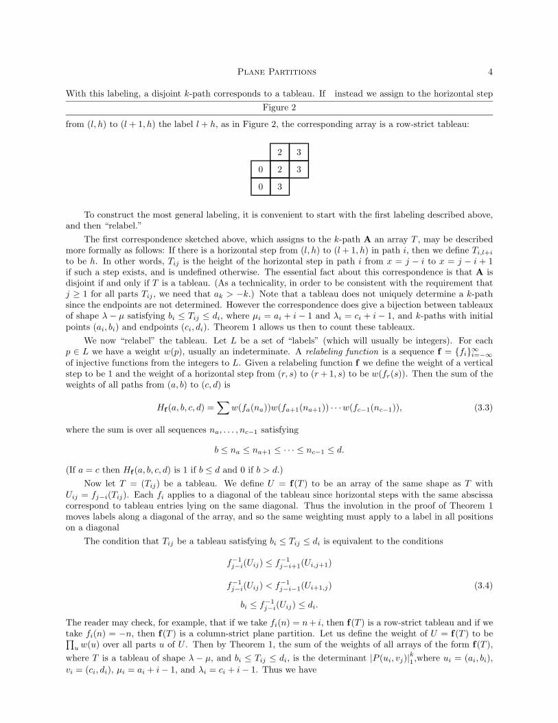
It is clear that a ∈ X1 and b ∈ X2, so X1 and X2 are nonempty. Now suppose that p ∈ X1 and q ∈ X2.To prove the theorem we need only show that p R q and q 6R p.
Plane Partitions 14
First we prove that p R q. We consider two cases. In the first case, we assume that q 6R q and a R q.We know that either a R p or p R a, by (i). If p R a then p R a R q, so by (iii), p R q. If a R p then we havep R p, since otherwise p would be in X2. Thus by (i), if p 6R q then q R p, so a R q R p, and thus p ∈ X2, acontradiction.
In the second case, there exists y with y 6R y and a R y R q. Then by the first case, we have p R y, sop R y R q. Then by (iii), p R q unless p R p. Thus by (i), if p 6R q then q R p and we have q R p R y, soq R y by (iii). Thus by (ii), y R y, a contradiction.
It remains to prove that q 6R p. But if q R p then since we have just shown that p R q, it follows from(ii) that q R q. Thus there must exist some y with y 6R y and a R y R q. Therefore we have y R q R p so by(iii), y R p. But since y ∈ X2, it follows from what we have already proved that p R y, so by (ii) we havey R y, a contradiction.
It follows that all semitransitive relations can be constructed from partial semiorders.The following construction shows that partial semiorders are easy to find: Start with a strict total order
< on X. Let f be function from X to X such that for all a, b ∈ X, f(a) ≥ a and a ≤ b implies f(a) ≤ f(b).Then let
R = { (a, b) | f(a) < b }. (7.3)
To see that R is semitransitive, suppose a R b R c but a 6R d. Then we have f(a) < b, f(b) < c, andf(a) ≥ d. Then d ≤ f(a) < b, so f(d) ≤ f(b) < c, and thus d R c. The condition f(a) ≥ a impies that Ris irreflexive. It is interesting to note that the number of such functions on an n-element set is the Catalannumber Cn. The relation on the integers given by a R b iff a ≤ b− t, where t ≥ 1, comes from the functionf(x) = x+ t− 1.
Not every partial semiorder is of this form; a counterexample is a disjoint union of two 2-element chains.To see this, note that if R is defined by (7.3), then the sets Rx = { y | x R y } over all x ∈ X are totallyordered by inclusion.
Edrei [18] (see also Karlin [34, p.412]) proved the following theorem, which was conjectured by Schoen-
berg (see [61]): Let rn be real numbers, with rn = 0 for n < 0. Then all determinants srλ/µ =∣∣rλi−µj+j−i∣∣k1
for all k are nonnegative if and only if
∞∑n=0
rnun = Cuλeγu
M∏i=1
(1 + αiu)/ N∏i=1
(1− βiu),
where αi, βi, and γ are positive real numbers, C ≥ 0,∑
(αi + βi) < ∞, and M and N may be infinite. Itfollows that for any finite partial semiorder R, if we set PR(u) =
∑i h
Ri u
i, then for any nonnegative valuesof the xi, PR(u) is a polynomial in u with negative roots.
The hook Schur functions give a strengthening of the easy half of Edrei’s theorem: if the αi, βi, and γare indeterminates, then srλ/µ has nonnegative coefficients as a polynomial in these variables. (The parameterγ can be accounted for via the homomorphism θ of Section 3, by introducing a third set of labels, each ofwhich can appear at most once.)
There is another way of looking at R-Schur functions: we can interpret them as evaluations of ordinarySchur functions. For the moment, let us think of hn, n ≥ 1, as indeterminates, with h0 = 1, and define theskew Schur functions sλ/µ as polynomials in the hn. Then sRλ/µ is the image of sλ/µ under the substitution
hn 7→ hRn . It follows that any polynomial identity among the sλ/µ remains true when sRλ/µ is substituted forsλ/µ. For example, we have the formulas
(h1)n =∑λ
fλsλ,
over all partitions λ of n, where fλ is the number of standard Young tableaux of shape λ, and
sµsν =∑ν
cλµνsλ,

Plane Partitions 15
where the integers cλµν are given by the Littlewood-Richardson rule [43, p. 68]. It is reasonable to expectthat these formulas can be explained combinatorially by analogs of the Robinson-Schensted correspondence[56, 59] and the jeu de taquin of Schutzenberger [62]. This has been done in the special case of the hookSchur functions by Remmel [52] and Worley [74].
8. Stanley’s formulaMuch of the theory of plane partitions is devoted to counting plane partitions or tableaux by the
sum of their entries. To accomplish this we set xi = qi in the formulas of Section 3. First we evaluatehn(xa, xa+1, . . . , xb) with xi = qi. Using the well-known expansions of (1 − z)(1 − zq) · · · (1 − zqn) and itsreciprocal [1, p. 19] we have
∞∑n=0
hn(qa, qa+1, . . . , qb)zn =1
(1− zqa) · · · (1− zqb)
=1
(zqa)b−a+1=∞∑j=0
zjqaj[b− a+ j
j
]and
∞∑n=0
en(qa, qa+1, , . . . , qb)zn = (1 + zqa) · · · (1 + zqb)
=b−a∏i=0
(1 + qizqa) =∑j
zjq(j2)+aj
[b− a+ 1
j
].
So
hn(qa, . . . , qb) = qan[b− a+ n
n
]and
en(qa, . . . , qb) = qan+(n2)[b− a+ 1
n
].
[Kreweras [39, p. 64] gave the determinant |(yi−y′j+ri−j+r
)| for counting r-tuples of paths between two given
paths of heights yi and y′j .]
Applying these formulas to Corollary 4, we obtain
Theorem 14. The generating function for tableaux of shape λ− µ in which parts in row i are at leastai and at most bi, where ai ≤ ai+1 and bi ≤ bi+1, is∣∣hλi−µj+j−i(qaj , . . . , qbi)∣∣k1 =
∣∣∣∣qaj(λi−µj+j−i)[bi − aj + λi − µj + j − iλi − µj + j − i
]∣∣∣∣k1
(8.1)
and the corresponding generating function for row-strict tableaux, where ai+1 − ai ≥ µi+1 − µi − 1 andbi+1 − bi ≥ λi+1 − λi − 1, is ∣∣∣∣qEij[ bi − aj + 1
λi − µj + j − i
]∣∣∣∣k1
,
where
Eij =(λi − µj + j − i
2
)+ aj(λi − µj + j − i). (8.2)
Analogous formulas for column-strict plane partitions are easily obtained from Theorem 14, since re-placing each entry with its negative changes a tableau to a column-strict plane partition. Then replacing ai
and bi with their negatives and q by q−1 in Theorem 14, and using the identity[n
k
]q−1
= q−k(n−k)
[n
k
]q
, we
obtain:

Plane Partitions 16
Theorem 15. The generating function for column-strict plane partitions of shape λ−µ in which partsin row i are at most ai and at least bi, where ai ≥ ai+1 and bi ≥ bi+1 is∣∣∣∣qbi(λi−µj+j−i)[aj − bi + λi − µj + j − i
λi − µj + j − i
]∣∣∣∣k1
. (8.3)
We can easily modify formula (8.3) to count (not necessarily column-strict) plane partitions: if we add ito every part in row i of a column-strict plane partition counted by (8.3), we increase the sum by
∑i(λi−µi)
and we obtain a plane partition of shape λ− µ in which parts in row i are at most ai + i and at least bi + i.Setting Ai = ai + i and Bi = bi + i, we obtain:
Theorem 16. The generating function for plane partitions of shape λ− µ in which parts in row i areat most Ai and at least Bi, where Ai ≥ Ai+1 − 1 and Bi ≥ Bi+1 − 1 is
qΣii(λi−µi)∣∣∣∣q(Bi−i)(λi−µj+j−i)
[Aj −Bi + λi − µjλi − µj + j − i
]∣∣∣∣k1
.
There are many determinants of q-binomial coefficients which have explicit formulas as quotients. Someof these are very difficult to evaluate [2–4, 6, 46, 47, 49?]. In this section we give an easy evaluation of adeterminant by induction, which yields a result of Stanley counting tableaux of a given shape with a givenmaximum part size. (For other work on evaluation of determinants of matrices of binomial and q-binomialcoefficients, see [10,29, 45, 48, and 69]. In the next section we use a simple summation formula to evaluatea determinant and give two (?) applications which seem to be new.
Let us consider the problem of counting tableaux of shape λ, with parts 0, 1, · · · , b−1. By formula (8.1)the generating function for these tableaux is∣∣∣∣[b+ λi + j − i
λi + j − i
]∣∣∣∣k1
.
However, in such a tableau the smallest part in row i must be at least i−1 (since µ = 0) so this determinantis also equal to∣∣∣∣q(j−1)(λi+j−i)
[b− 1− (j − 1) + λi + j − i
λi + j − i
]∣∣∣∣k1
=∣∣∣∣q(j−1)(λi+j−i)
[b+ λi − iλi + j − i
]∣∣∣∣k1
, (8.4)
and this determinant turns out to be easier to evaluate.We now define the hook lengths and contents of a diagram. The hook length of a square in a diagram
is the number of squares to its right plus the number of squares below it plus one. Thus the hook length ofsquare (i, j) is λi + λ′j − i− j + 1. The content of square (i, j) is j − i. The hook lengths and contents of thediagram for the partition (431) are as follows:
6 4 3 1
4 2 1
1
Hook lengths
0 1 2 3
−1 0 1
−2
Contents
We write h(x) and c(x) for the hook length and content of x, and we set H(λ) =∏x(1 − qh(x)) and
Ca(x) =∏x(1− qa+c(x)), where the product is over all squares x of the diagram of λ.

Plane Partitions 17
Theorem 17. (Stanley [65]) The generating function for tableaux of shape λ with parts 0, 1, · · · , b− 1is qeCb(λ)/H(λ), where e =
∑ki=1(i− 1)λi.
Proof. We evaluate the determinant (8.4) by induction. First note that if λk = 0 (8.4) reduces to theformula for λ1, λ2, · · · , λk−1.
Now first suppose that b is greater than k, the number of parts of λ. Note that
Cb(λ) = Cb−1(λ)(1− qb+λ1−1)(1− qb+λ2−2) · · · (1− qb+λk−k)
(1− qb−1)(1− qb−2) · · · (1− qb−k).
Then by induction the determinant is∣∣∣∣q(j−1)(λi+j−i)[b+ λi − ib− j
]∣∣∣∣ =∣∣∣∣q(j−1)(λi+j−i) 1− qb+λi−i
1− qb−j[b+ λi − i− 1b− j − 1
]∣∣∣∣=
k∏i=1
(1− qb+λi−i)(1− qb−i) · qeCb−1(λ)
H(λ)= qe
Cb(λ)H(λ)
.
If b = k and λk 6= 0 then the first column must be 0, 1, 2, . . . , b − 1. So the tableau is determined bythe entries in columns 2, 3, . . . , λ1, which may constitute an arbitrary tableau of shape λ = (λ1 − 1, λ2 −1, · · · , λk − 1). Thus by induction the generating function is
q0+1+···+(k−1)q(λ2−1)+2(λ3−1)+···+(k−1)(λk−1)Cb(λ)H(λ)
= qeCb(λ)H(λ)
.
Now H(λ) = H(λ) · (1 − qλ1+k−1)(1 − qλ2+k−2) · · · (1 − qλk) and Cb(λ) = Cb(λ) ·(1− qb+λ1−1) · · · (1− qb+λk−k) and thus when b = k,
Cb(λ)H(λ)
=Ck(λ)H(λ)
=Ck(λ)H(λ)
=Cb(λ)H(λ)
.
9. Some quotient formulasNext we consider some determinants of binomial coefficients which can be evaluated explicitly. For
simplicity, we consider here only the case q = 1.We use the notation (a)n to denote a(a+ 1) · · · (a+ n− 1).
Lemma 18. ∣∣∣∣ 1(αi)j
∣∣∣∣n0
=
∏0≤i<j≤n
(αi − αj)
n∏i=0
(αi)n
Proof. The formula is equivalent to∣∣∣∣ (αi)n(ai)j
∣∣∣∣n0
=∏
0≤i<j≤n(αi − αj)
The left side is|(αi + j)(αi + j + 1) · · · (αi + n− 1)|n0 .
Since the entries in column j of this determinant are the values of a polynomial of degree n− j evaluated atthe points αi, elementary column operations reduce this to a Vandermonde determinant.
Plane Partitions 18
Lemma 19.
∣∣∣∣ (αi − βj)j(αi)j
∣∣∣∣n0
=
n∏i=0
(βi)i∏
0≤i<j≤n(αj − αi)
n∏i=0
(αi)n
.
Proof. Let A be the matrix(
1(αi)j
)and let B be the matrix
((βj)i(−j)i
i!
). Then the (i, j) entry of
C = AB isn∑l=0
1(αi)l
(βj)l(−j)ll!
=(αi − βj)j
(αi)j
by Vandermonde’s theorem [5, p. 3]. Thus |C| = |A||B|. Since B is upper triangular,
|B| =n∏j=0
(βj)j(−j)jj!
= (−1)(n2)
n∏j=0
(βj)j
and the result follows from 18
We now give two applications of Lemma 19. First let us evaluate the determinant∣∣∣(β−αi+jαi+j−1
)∣∣∣n0. Since
(αi − β − j)j = (−1)j(β − αi + 1)j , we have
(β − αi + j
αi + j − 1
)=(β − αiαi − 1
)(β − αi + 1)j
(αi)j
= (−1)j(β − αi)!
(β − 2αi + 1)! (αi − 1)!(αi − β − j)j
(αi)j.
Thus ∣∣∣∣(β − αi + j
αi + j − 1
)∣∣∣∣n0
= (−1)(n+1
2 )n∏i=0
(β − αi)! (β + i)i(β − 2αi + 1)! (αi − 1)! (αi)n
∏0≤i<j≤n
(αj − αi)
=n∏i=0
(β − αi)! (β + i)i(β − 2αi + 1)! (αi − 1)! (αi)n
∏0≤i<j≤n
(αi − αj)
=n∏i=0
(β − αi)! (β + i)i(β − 2αi + 1)! (αi + n− 1)!
∏0≤i<j≤n
(αi − αj). (9.1)
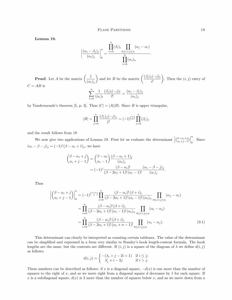
This determinant can clearly be interpreted as counting certain tableaux. The value of the determinantcan be simplified and expressed in a form very similar to Stanley’s hook length-content formula. The hooklengths are the same, but the contents are different. If (i, j) is a square of the diagram of λ we define d(i, j)as follows:
d(i, j) ={−(λi + j − 2i+ 1) if i ≤ j;
λ′j + i− 2j if i > j.
These numbers can be described as follows: if x is a diagonal square, −d(x) is one more than the number ofsquares to the right of x, and as we move right from a diagonal square d decreases by 1 for each square. Ifx is a subdiagonal square, d(x) is 2 more than the number of squares below x, and as we move down from a

Plane Partitions 19
subdiagonal square, d increases by 1 for each square. Here are the values of d(i, j) for the partition (44331):
−5 −6 −7 −8 −9
5 −4 −5 −6 −7
6 4 −1
7 5 2
8 6
In this section we let H(λ) be the product of the hook lengths of λ. We will need the following lemma (seeMacdonald [43, p. 9]):
Lemma 20. For any partition λ,
∏1≤i<j≤k
(λi − λj − i+ j)
k∏i=1
(λi − i+ k)!
=1
H(λ).
Theorem 21. The number of tableaux of shape λ with positive integer parts, in which the largest partin row i is at most r − 2λi + 2i− 1 is
1H(λ)
∏x∈λ
(r + d(x)
).
Proof. In (9.1) we set αi = λi+1 − i+ 1, k = n+ 1, and β = r+ 1. When i and j are replaced by i− 1and j − 1, the determinant becomes ∣∣∣∣(r − λi + i+ j − 2
λi − i+ j
)∣∣∣∣k1
,
and the combinatorial interpretation follows from Theorem 14. The value of the determinant is
k∏i=1
(r − λi + i− 1)! (r + i)i−1
(r − 2λi + 2i− 2)! (λi − i+ k)!
∏1≤i<j≤k
(λi − λj + j − i)
=1
H(λ)
k∏i=1
(r + 2i− 2)(r + 2i− 3) · · · (r + 2i− 2λi − 1)(r + i− 1)(r + i− 2) · · · (r + i− λi)
=1
H(λ)
k∏i=1
λi∏j=1
(r + 2i− 2j)(r + 2i− 2j − 1)(r + i− j)
=1
H(λ)
∏(i,j)∈λ
(r + 2i− 2j)(r + 2i− 2j − 1)(r + i− j)
We break the product into two factors.

Plane Partitions 20
First we have
∏(i,j)∈λi≤j
(r + 2i− 2j)(r + 2i− 2j − 1)(r + i− j) =
k∏i=1
λi−i∏l=0
(r − 2l)(r − 2l − 1)(r − l)
=k∏i=1
2λi−2i+1∏m=0
(r −m)
λi−i∏n=0
(r − n)
=k∏i=1
2λi−2i+1∏m=λi−i+1
(r −m).
With the substitution m = j + λi − 2i+ 1, this becomes
k∏i=1
λi∏j=i
(r − j − λi + 2i− 1) =∏x∈λ+
(r + d(x)
).
Next we have, with k′ = λ1
∏(i,j)∈λi>j
(r + 2i− 2j)(r + 2i− 2j − 1)(r + i− j) =
k′∏j=1
λ′j−j∏l=1
(r + 2l − 1)(r + 2l)(r + l)
=k′∏j=1
2λ′j−2j∏m=1
(r +m)
λ′j−j∏n=1
(r + n)
=k′∏j=1
2λ′j−2j∏m=λ′
j−j+1
(r +m).
With the substitution m = i+ λ′j − 2j,
k′∏j=1
λ′j∏i=j+1
(r + i+ λ′j − 2j) =∏x∈λ−
(r + d(x)
),
completing the proof.
Another determinant we can evaluate using Lemma 19 is∣∣Ci+αj ∣∣n0 , where Cn is the Catalan number
defined by
Cn =1
n+ 1
(2nn
)= 22n (1/2)n
(2)n.
Since
Ci+αj = 22i+2αj(1/2)i+αj(2)i+αj
= 22i+2αj(1/2)αj (1/2 + αj)i
(2)αj (2 + αj)i,

Plane Partitions 21
the determinant is equal to
2n(n+1)+2Σjαj
∏j(1/2)αj∏j(2)αj
∣∣∣∣ (1/2 + αj)i(2 + αj)i
∣∣∣∣n0
Now by the lemma ∣∣∣∣ (1/2 + αj)i(2 + αj)i
∣∣∣∣n0
=∏ni=0(3/2)i∏n
j=0(αj + 2)n
∏0≤i<j≤n
(αj − αi).
Simplifying, we find that the determinant is
∏0≤i<j≤n
(αj − αi)n∏j=0
(2αj)!αj ! (αj + n+ 1)!
n∏i=0
(2i+ 1)!i!
.
See Viennot [71] for an evaluation of a special case of this determinant, using the qd-algorithm of Padeapproximant theory. See also de Sainte-Catherine and Viennot [14].
We recall that Ci is the number of paths from (0, 0) to (2i, 2i) which never go above (but may touch)the line x = y.
Now assume that 0 ≤ α0 < α1 < · · · < αn and let the points Pi and Qi be defined by Pi(n − i, n − i)and Qi = (n+ αi, n+ αi) for i = 0, . . . , n. If we consider the digraph of lattice points with only those stepsthat lie below the line x = y, then (P,Q) is nonpermutable. Thus the determinant |Ci+αj |n0 is the numberof disjoint (n+ 1)-paths from P to Q.
These paths may be expressed as tableaux: we consider separately the cases α0 = 0 and α0 6= 0.
First we consider the case α0 = 0. In Figure 6 an example with α0 = 0, α1 = 2, and α2 = 5 is given.Figure 6
It is clear that path i begins with 2i horizontal steps, and thus we may remove these steps, and associatewhat remains with a tableau in the usual way. Thus Figure 6 corresponds to the tableau
1 1 6
2
In general, the tableau will have shape (αn − n, αn−1 − n + 1, . . . , α1 − 1). The requirement that all stepsfall below the main diagonal is equivalent to the condition that pij ≤ 2n + j − i. This condition is impliedby the inequalities for the last elements in each column.
If we make the substitution λi = αn+1−i− (n+ 1− i), (so that αi = λn+1−i + i) for i = 1, . . . , n and setk = n, then we obtain the following:
Theorem 22. The number of tableaux (pij) of shape λ with nonnegative entries satisfying pij ≤2k + j − i, or equivalently, pλ′
j,j ≤ 2k + j − λ′j , is
1(k + 1)!
k∏i=1
(λi + k − i+ 1)!∏
1≤i<j≤k(λi − λj − i+ j)
k∏i=1
(2λi + 2k − 2i+ 2)!(λi + k − i+ 1)! (λi − i+ 2k + 2)!
k∏i=0
(2i+ 1)!i!
.
Plane Partitions 22
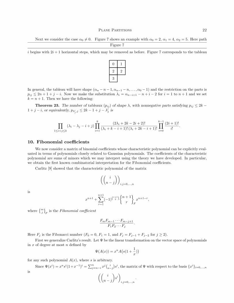
Next we consider the case α0 6= 0. Figure 7 shows an example with α0 = 2, α1 = 4, α2 = 5. Here pathFigure 7
i begins with 2i+ 1 horizontal steps, which may be removed as before. Figure 7 corresponds to the tableau
0 1
2 2
3
In general, the tableau will have shape (αn − n− 1, αn−1 − n, . . . , α0 − 1) and the restriction on the parts ispij ≤ 2n + 1 + j − i. Now we make the substitution λi = αn−i+1 − n + i − 2 for i = 1 to n + 1 and we setk = n+ 1. Then we have the following:
Theorem 23. The number of tableaux (pij) of shape λ, with nonnegative parts satisfying pij ≤ 2k −1 + j − i, or equivalently, pλ′
j,j ≤ 2k − 1 + j − λ′j is
∏1≤i<j≤k
(λi − λj − i+ j)k∏i=1
(2λi + 2k − 2i+ 2)!(λi + k − i+ 1)! (λi + 2k − i+ 1)!
k−1∏i=0
(2i+ 1)!i!
.
10. Fibonomial coefficientsWe now consider a matrix of binomial coefficients whose characteristic polynomial can be explicitly eval-
uated in terms of polynomials closely related to Gaussian polynomials. The coefficients of the characteristicpolynomial are sums of minors which we may interpret using the theory we have developed. In particular,we obtain the first known combinatorial interpretation for the Fibonomial coefficients.
Carlitz [9] showed that the characteristic polynomial of the matrix((i
n− j
))i,j=0,...,n
is
xn+1 +n+1∑r=1
(−1)(r+1
2 ){n+ 1r
}F
xn+1−r,
where{mj
}F
is the Fibonomial coefficient
FmFm−1 · · ·Fm−j+1
F1F2 · · ·Fj.
Here Fj is the Fibonacci number (F0 = 0, F1 = 1, and Fj = Fj−1 + Fj−2 for j ≥ 2).First we generalize Carlitz’s result. Let Ψ be the linear transformation on the vector space of polynomials
in x of degree at most n defined by
Ψ(A(x)) = xnA(s(1 +
1x
))
for any such polynomial A(x), where s is arbitrary.
Since Ψ(xi) = xnsi(1+x−1)i =∑nj=n−i x
j(
in−j)si, the matrix of Ψ with respect to the basis {xi}i=0,...,n
is ((i
n− j
)si)i,j=0,...,n
.

Plane Partitions 23
Now we have
Ψ((1 + ax)k(1 + bx)n−k
)= (as)k(bs)n−k
(1 +
1 + as
asx
)k (1 +
1 + bs
bsx
)n−k.
Thus if (1 + as)/as = a and (1 + bs)/bs = b, i.e.,
a, b =s±√s2 + 4s2s
then (1 + ax)k(1 + bx)n−k will be an eigenvector for Ψ with eigenvalue (as)k(bs)n−k. As long as s2 + 4s 6= 0these will be distinct for k = 0, . . . , n, and thus give all the eigenvalues of Ψ.
By continuity, we may remove the restriction on s and we obtain:
Theorem 24. The eigenvalues of the matrix M =((
i
n− j
)si)i,j=0,...,n
are αkβn−k, k = 0, . . . , n,
where
α, β =s±√s2 + 4s2
,
and thus the characteristic polynomial of M is
|(xI −M)| =n∏k=0
(x− αkβn−k) (10.1)
where I is the identity matrix.
To express the product simply, it is convenient to introduce the homogeneous Gaussian polynomials,defined by [
m
j
]p,q
=(pm − qm)(pm−1 − qm−1) · · · (pm−j+1 − qm−j+1)
(p− q)(p2 − q2) · · · (pj − qj) .
These are related to the ordinary Gaussian polynomials by[m
j
]p,q
= qmj−j2[m
j
]p/q
.
Then the following formula is equivalent to a form of the q-binomial theorem:
n∏k=0
(x+ pkqn−k) =n+1∑k=0
xn+1−k(pq)(k2)[n+ 1k
]p,q
.
Thus by (10.1), we have
|(xI −M)| =n+1∑k=0
xn+1−k(−1)(k+1
2 )s(k2)[n+ 1k
]α,β
, (10.2)
since αβ = −s.Now let Gn = (αn − βn)/(α− β). The following facts about Gn are easily verified:
G0 = 0, G1 = 1, and Gn = s(Gn−1 +Gn−2)∞∑n=0
Gnun =
u
1− s(u+ u2)
Gn =n∑
i=dn/2esi(
i
n− i
).

Plane Partitions 24
Note that for s = 1, Gn reduces to Fn. Let us define{mj
}to be
[mj
]α,β
, so that{m
j
}=GmGm−1 · · ·Gm−j+1
G1G2 · · ·Gj.
We note that from the easily proved formula Gm+n = GmGn+1 + sGm−1Gn we obtain the recurrence{m
j
}= Gm−j+1
{m− 1j − 1
}+ sGj−1
{m− 1j
}(10.3)
We now turn to the combinatorial interpretation. We know that the coefficient of xn+1−k in |(xI −M)|is (−1)k times the sum of all the k × k principal minors of M , i.e., the minors obtained by choosing k rowsand the same k columns from M . Such a minor is a determinant∣∣∣∣( ri
n− rj
)sri∣∣∣∣k1
. (10.4)
To get a determinant in the form we can interpret, we reverse the order of the columns in (10.4); then (10.4)
is equal to (−1)(k2)sΣri times the determinant∣∣∣∣( ri
n− rk+1−j
)∣∣∣∣k1
(10.5)
The determinant (10.5) is easily interpreted by our theory. It is in fact a binomial determinant , as studiedin Gessel and Viennot [25], and it has the following interpretation: define points Pi and Qi by Pi = (0,−i)and Qi = (−n + i,−n + i). For any subset R = {r1 < r2 < · · · < rk} of {0, 1, . . . , n}, let N(R) be the
number of nonintersecting k-paths from (Pr1 , · · · , Prk) to (Qrk , · · · , Qr1). Then∣∣∣( rin−rk+1−j
)∣∣∣ = N(R).
Theorem 25. For any subset R of {0, 1, . . . , n} let ‖R‖ =∑i∈R i and let N(R) be defined as above.
Then ∑R
s‖R‖N(R) = s(k2){n+ 1k
},
where the sum is over all k-subsets R of {0, 1, . . . , n}.
Several questions related to Theorem 15 present themselves. First it would be nice to have a more naturalinterpretation than the one we have given. Second, is there a combinatorial interpretation to the recurrence(10.3)? R. Stanley has asked if there is a binomial poset associated with the Fibonomial coefficients; i.e., aranked poset such that for all x and y in the poset if x < y and r(y)− r(x) = n then there are exactly
{nk
}F
points z with x < z < y and r(z)− r(x) = k. Our work constructs the right number of objects, but it is notclear how to partially order them to obtain such a binomial poset.
11. Jacobi’s theoremThere is a theorem of Jacobi [32; 41, p. 153–156] which relates the minors of a matrix to minors of
the inverse matrix. It may be stated in the following form: Let M be an invertible matrix with rows andcolumns indexed by some set I = {a, a+ 1, · · · , a+ n}. (In our applications, a is 0 or 1.) Let L = M−1. Weshall call the matrix M∗ =
((−1)i+jLij
)the sign-inverse of M .
If A and B are subsets of I of the same size, let M [A|B] denote the minor of M corresponding to therows in A and the columns in B. Jacobi’s theorem asserts that if N is the sign-inverse of M then
M [A|B] = |M | ·N [I −B|I −A] (11.1).
In many cases, especially when M is a triangular matrix with 1’s on the diagonal, (11.1) can be inter-preted combinatorially. See, for example, Gessel and Viennot [25, Section 4].
One of the simplest examples is the case in which M is the matrix (hi−j). It is easily verified thatM∗ = (ei−j). Then Jacobi’s theorem gives the expression of a skew Schur function in terms of the ei.
The following theorem gives a pair of sign-inverse matrices to which we can apply Jacobi’s theorem.

Plane Partitions 25
Lemma 26. Let a0, a1, . . . and b0, b1, . . . be arbitrary, and define pi and qi by
∞∑i=0
piui =
( ∞∑i=0
(−1)iaiui)−1
and∞∑i=0
qiui =
( ∞∑i=0
(−1)ibiui)/( ∞∑
i=0
(−1)iaiui)
Then
(i) The matrices (aj−i) and (pj−i) are sign-inverse (where ak = pk = 0 for k < 0),
(ii) The matrices
U =
1 b0 b1 · · · bn0 a0 a1 · · · an0 0 a0 · · · an−1
......
......
0 0 0 · · · a0
and
V =
1 q0 q1 · · · qn0 p0 p1 · · · pn0 0 p0 · · · pn−1
......
......
0 0 0 · · · p0
are sign-inverse.
The proof is straightforward.Now let us take ai = him+r for fixed m and r, where 0 ≤ r < m, and bi = him+s. Then
∞∑i=0
piui =
( ∞∑i=0
him+rui
)−1
and
∞∑i=0
qiui =
∞∑i=0
(−1)ihim+sui
∞∑i=0
(−1)ihim+rui
.
(The variable u is actually redundant in these formulas.) The significance of the restriction 0 ≤ r < m isthat it implies that the sum could as well start at −∞ instead of at 0.[why?]
Before we apply Jacobi’s theorem we need to relate complements of sets to conjugate partitions. Byreasoning as in Macdonald [43, p. 15; see also (1.7), p. 3] it follows from Jacobi’s theorem that if λ and µare two partitions with at most s parts and largest part at most t, where s + t = w, and if M and N aresign-inverse matrices with rows and columns indexed 0, 1, . . . , w, then we have
M [{λi + s− i}1≤i≤s|{µj + s− j}1≤j≤s] = |M | ·N [{s− 1 + i− µ′i}1≤i≤t|{s− 1 + j − λ′j}1≤j≤t]
Now since sλ/µ =∣∣hλi−µj+j−i∣∣ we have for the symmetric functions pi
|pλi−µj−i+j | = h−(s+t)r |h(λ′
i−µ′
j−i+j)m+r|1≤i,j≤t = h−(s+t)
r sλ/µ,
Plane Partitions 26
whereλi = mλ′i − (m− 1)i+ r + C
µi = mµ′i − (m− 1)i+ C
where C is large enough to make λ and µ nonnegative.The simplest case is that in which λ = (n), µ = ∅. So λ′i = 1 for i = 1, . . . , n. We may take s = 1, t = n.
We getλi = m− (m− 1)i+ r + C, i = 1, . . . , n
µi = −(m− 1)i+ C, i = 1, . . . , n.
We may take C = (m− 1)n, and we obtain
λi = (m− 1)(n− i) +m+ r
µi = (m− 1)(n− i).(11.2)
Thus λi − µi = m+ r and λi+1 − µi = r + 1.
Figure 8
Applying the homomorphism θ of Section 2 and setting u = 1 we get( ∞∑n=0
(−1)nxmn+r
(mn+ r)! (xr/r!)n−1
)−1
(11.3)
as the exponential generating function for Young tableaux of shape λ − µ given by (11.2). For example, ifm = 2 and r = 1 (11.3) reduces to x3/2/ sin(x3/2). Since
x
sinx=∞∑n=0
dnx2n
(2n)!,
where dn is related to the Bernoulli number by dn = (−1)n+1(22n − 2)B2n, it follows that
x3/2
sin(x3/2)=∞∑n=0
dn(3n)!(2n)!
x2n
(2n)!
and thus(3n)!(2n)!
dn is the number of Young tableaux of shape (n + 2, n + 1, . . . , 3) − (n − 1, n − 2, . . . , 0).
This result may be compared with a combinatorial interpretation of 1 · 3 · · · (2n+ 1)d2n given in Gessel andViennot [25, p. 315].
12. Salie numbers and Faulhaber numbersIn view of Jacobi’s theorem, it is natural to ask when matrices of binomial coefficients to which our
theory applies have inverses which can be expressed in some kind of explicit form. In this section we discussa closely related pair of such matrices. The entries of their inverses are numbers which have arisen in othercontexts, but are not well known. One of them, according to Edwards [17], was studied by Faulhaber [20]in the seventeenth century in connection with formulas for sums of powers. The other was apparently firstconsidered by Salie [58] in 1963 in connection with the number-theoretic properties of the coefficients ofcosh z/ cos z. (See also Hammersley [ ] and Dumont and Zeng [16].)
Both arrays of numbers can be defined in three ways: as entries of the inverse of a matrix of binomialcoefficients, by generating functions, and by formulas for sums of powers. We shall start with the generatingfunctions.

Plane Partitions 27
We define the Salie numbers s(n, k) by
∞∑n,k=0
s(n, k)tkx2n
(2n)!=
cosh√
1 + 4tx2cosh x
2
(12.1)
and we define the Faulhaber number f(n, k) by
∞∑n,k=0
f(n, k)tkx2n+1
(2n+ 1)!=
cosh√
1 + 4tx2 − cosh x2
t sinh x2
. (12.2)
It is easily seen that s(n, k) = f(n, k) = 0 for k > n. As we shall see later, |s(n, k)| = (−1)n−ks(n, k)and |f(n, k)| = (−1)n−kf(n, k). The first few values of these numbers are as follows (zeros are omitted):
s(n, k) : n\k 0 1 2 3 40 11 12 −1 13 3 −3 14 −17 17 −6 15 155 −155 55 −10 16 −2073 2073 −736 135 −15 17 38227 −38227 13573 −2492 280 −21 1
f(n, k) : n\k 0 1 2 3 4 5 6 70 11 1/22 −1/6 1/33 1/6 −1/3 1/44 −3/10 3/5 −1/2 1/55 5/6 −5/3 17/12 −2/3 1/66 −691/210 691/105 −118/21 41/15 −5/6 1/77 35/2 −35 359/12 −44/3 14/3 −1 1/8
Next we prove the sums of powers formulas. Let Sr(m) =∑mi=0 i
r, with 00 = 1, so that S0(m) = m+ 1.
Theorem 27.
S2n+1(m) =12
n∑k=0
f(n, k)(m(m+ 1)
)k+1. (12.3)
Proof. We have
∞∑r=0
Sr(m)xr
r!= 1 + ex + · · ·+ emx =
e(m+1)x − 1ex − 1
=e(m+ 1
2 )x − e−x/2ex/2 − e−x/2 =
sinh(m+ 12 )x+ cosh(m+ 1
2 )x+ sinh x2 − cosh x
2
2 sinh x2
.
Thus∞∑n=0
S2n+1(m)x2n+1
(2n+ 1)!=
cosh(m+ 12 )x− cosh x
2
2 sinh x2
.

Plane Partitions 28
Now set t = m(m+ 1), so√
1 + 4t = 2m+ 1. Then∞∑n=0
S2n+1(m)x2n+1
(2n+ 1)!=
cosh√
1 + 4tx2 − cosh x2
2 sinh x2
=t
2
∞∑n,k=0
f(n, k)tkx2n+1
(2n+ 1)!
=12
∞∑n=0
x2n+1
(2n+ 1)!
n∑k=0
f(n, k)(m(m+ 1)
)k+1,
and the result follows by equating coefficients ofx2n+1
(2n+ 1)!.
Formula (12.3) was first studied by Faulhaber [20] in the seventeenth century. Faulhaber’s work isdescribed in Edwards [17] Schneider [60], and Knuth . Formula (12.3) was rediscovered by Jacobi [33], whogave the recurrence (in our notation)
2n(2n+ 1)f(n− 1, k − 2) = 2k(2k − 1)f(n, k − 1) + k(k + 1)f(n, k).
[Give analogous formula for Salie numbers, from Concrete Math. 7.52] As far as we know, the generatingfunction (12.2) is new.
There is a companion formula which we state for completeness, although we will not use it (see Edwards[17]):
S2n(m) = (m+12
)n∑k=0
f(n, k)(m(m+ 1)
)k,
for n > 0, where
1 +∞∑n=1
x2n
(2n)!
n∑k=0
f(n, k)tk =sinh√
1 + 4tx2√1 + 4t sinh x
2
,
and moreover,
f(n, k) =k + 12n+ 1
f(n, k).
Next we consider the analogous formula for Salie numbers. Let
Tr(m) =12
m∑i=−m
(−1)m−iir,
so if r is odd Tr(m) = 0, and for n > 0,
T2n(m) =m∑i=1
(−1)m−ii2n.
Theorem 28.
T2n(m) =12
n∑k=0
s(n, k)(m(m+ 1)
)k.
Proof. We have
12
∞∑r=0
(m∑
i=−m(−1)m−iir
)xr
r!=
12
m∑i=−m
(−1)m−ieix =ex(m+ 1
2 ) + e−x(m+ 12 )
2(ex/2 + e−x/2)
=cosh(m+ 1
2 )x2 cosh x
2
=cosh
√1 + 4tx2
2 cosh x2
=12
∞∑n,k=0
s(n, k)x2n
(2n)!tk

Plane Partitions 29
and the theorem follows by equating coefficients ofx2n
(2n)!.
There is a companion formula for∑2n+1i=1 (−1)m−ii2n+1 that we leave to the reader.
Next we relate the Faulhaber and Salie numbers to inverses of matrices of binomial coefficients.
Theorem 29. The inverse of the matrix
((i+ 1
2i− 2j + 1
))i,j=0,···m
is the matrix(f(i, j)
)i,j=0,···m, and
the inverse of the matrix
((i
2i− 2j
))i,j=0,···m
is the matrix(s(i, j)
)i,j=0,···m.
Proof. We have (i(i+ 1)
)r+1 −((i− 1)i
)r+1 = 2∑l odd
(r + 1l
)i2r+2−l.
Summing on i from 0 to m we obtain
(m(m+ 1)
)r+1 = 2∑l odd
(r + 1l
)S2r+2−l(m) = 2
r∑j=0
(r + 1
2r − 2j + 1
)S2j+1(m)
and the first assertion follows from Theorem 27.Similarly, we have (
i(i+ 1))r +
((i− 1)i
)r = 2∑l even
(r
l
)i2r−l.
Multiplying by (−1)m−i, summing from i = −m to m, and dividing by 2, we obtain
(m(m+ 1)
)r = 2∑l even
(r
l
)T2r−l(m) = 2
r∑j=0
(r
2r − 2j
)T2j(m)
and the second assertion follows from Theorem 28.The proof just given follows Edwards [17] (who considered only the Faulhaber numbers).
Note that since the matrix(
i
2i− 2j
)is lower triangular with 1’s on the diagonal, its inverse has integer
entries, so the Salie numbers are integers. We can now explain Salie’s interest in these numbers [58]. (Seealso Comtet [13, pp. 86–87].) Salie was studying the numbers S2n defined by
coshxcosx
=∞∑n=0
S2nx2n
(2n)!.
In equation (12.1) if we replace x by 2ix, where i =√−1, and set t = −1
2 we obtain
coshxcosx
=∞∑n=0
22n(−1)nx2n
(2n)!
n∑k=0
s(n, k)(−12
)k
and thus
S2n = 22n(−1)nn∑k=0
s(n, k)(−1
2
)k=
n∑k=0
s(n, k)(−1)n−k22n−k.
Thus S2n is divisible by 2n, as shown by Salie. (Salie used the notation c(i)i−j for our s(i, j).)

Plane Partitions 30
It follows from equation (12.4) below that s(n, n) = 1, s(n, n − 1) = −(n
2
), and s(n, n − 2) =(
n− 12
)(n
2
)−(n
4
), so that we have in fact,
2−nS2n ≡ 1 + 2(n
2
)+ 4(n− 1
2
)(n
2
)− 4(n
4
)(mod 8).
Salie obtained a congruence (mod 16) for the numbers 2−nS2n by a different method. See also Carlitz [8].Next we consider the combinatorial interpretation of the Salie numbers and Faulhaber numbers. First
we note the following lemma, which follows easily from the formula for the inverse of a matrix.
Lemma 30. Let(Aij)i,j=0,...,m
be an invertible lower triangular matrix, and let (Bij) = (Aij)−1. Then
for 0 ≤ k ≤ n ≤ m, we have
Bn,k =(−1)n−k
Ak,kAk+1,k+1 · · ·An,n|Ak+i+1,k+j |i,j=0,...,n−k−1 .
Since the Salie numbers are entries of((
i
2i− 2j
))−1
, we have
s(n, k) = (−1)n−k∣∣∣∣( k + i+ 1
2i− 2j + 2
)∣∣∣∣n−k−1
0
(12.4)
and since the Faulhaber numbers are entries of((
i+ 12i− 2j + 1
))−1
, we have
f(n, k) = (−1)n−kk!
(n+ 1)!
∣∣∣∣( k + i+ 22i− 2j + 3
)∣∣∣∣n−k−1
0
. (12.5)
Although we can give a combinatorial interpretation of these determinants using Theorem 14, thesimplest interpretations are most easily derived directly from the paths.
For the Salie numbers, we define the points Pm = (2m,−2m) and Qm = (2m,−m). Then it fol-lows from (12.4) that (−1)n−ks(n, k) is the number of disjoint (n − k)-paths from (Pk, Pk+1, . . . , Pn−1) to(Qk+1, Qk+2, . . . , Qn). Figure 9 illustrates a 3-path counted by |s(5, 2)|. We note that it is immediate from
Figure 9
this combinatorial interpretation that |s(n, 1)| = |s(n, 2)|. To represent these (n − k)-paths most simply astableaux, we assign to the horizontal segment from (i,−j) to (i + 1,−j) the label i − j + 1 and make thelabels on each path into a row of the tableau, shifting as usual. Thus the 3-path of Figure 9 becomes thetableau
3 5
2 4
1 2
(12.6)
Converting the conditions on the paths into conditions on the tableau, we have
Theorem 31. |s(n, k)| = (−1)n−ks(n, k) is the number of row-strict tableaux of shape (n− k + 1, n−k, . . . , 2)− (n− k − 1, n− k − 2, . . . , 0) with positive integer entries in which the largest entry in row i is atmost n+ 1− i.
We may convert the tableau into a sequence of integers by reading each row from left to right, startingwith the last row, so that (12.6) becomes 1 2 2 4 3 5. Checking the conditions on this sequence, we find that we

Plane Partitions 31
are counting sequences a1a2 · · · a2n−2k of positive integers satisfying a2i−1 < a2i, a2i ≥ a2i+1, and a2i ≤ k+ ifor each i. This combinatorial interpretation is closely related to the combinatorial interpretation of theGenocchi numbers given by Dumont and Viennot [15]. See also Viennot [70].
Next we move on the Faulhaber numbers. Let Pm = (2m,−2m) as before, and let Rm = (2m+ 1,−m).
Then (−1)n−k(n+ 1)!k!
f(n, k) is the number of nonintersecting (n − k)-paths from (Pk, Pk+1, . . . , Pn−1) to
(Rk+1, Rk+2, . . . , Rn). As in the case of the Salie numbers, we represent these (n− k)-paths as tableaux,
Figure 10
so the 4-path of Figure 10 becomes
1 3 5
3 4 5
1 3 4
1 2 3
(12.7)
and we have
Theorem 32. (−1)n−k(n+ 1)!k!
f(n, k) is the number of row-strict tableaux of shape (n−k+ 2, n−k+
1, . . . , 2)− (n− k − 1, n− k − 2, . . . , 0) with positive integer entries in which the largest entry in row i is atmost n+ 2− i.
We can also represent these tableaux as sequences, so for example, (12.7) becomes 1 2 3 1 3 4 3 4 5 1 3 5,and we have
Theorem 33. (−1)n−k(n+ 1)!k!
f(n, k) is the number of sequences a1a2 · · · a3n−3k of positive integers
satisfying a3i−2 < a3i−1 < a3i, a3i−1 ≥ a3i+1, a3i ≥ a3i+2, and a3i ≤ k + i+ 1 for all i.
We now derive some explicit formulas for the Salie numbers in terms of the Genocchi numbers, and forthe Faulhaber numbers in terms of the Bernoulli numbers.
We first consider the Salie numbers. We shall need the formula [55, Ex. 2, pp. 153–154](1−√
1 + 4t2
)i=∞∑k=i
i
2k − i
(2k − ik
)(−t)k. (12.8)
Now
cosh√
1 + 4tx
2= cosh
((1−√
1 + 4t2
)x− x
2
)= cosh
(1−√
1 + 4t2
)x cosh
x
2− sinh
(1−√
1 + 4t2
)x sinh
x
2so
cosh√
1 + 4tx2cosh x
2
=∞∑j=0
x2j
(2j)!
∞∑k=2j
2j2k − 2j
(2k − 2j
k
)(−t)k
− tanhx
2
∞∑j=0
x2j+1
(2j + 1)!
∞∑k=2j+1
2j + 12k − 2j − 1
(2k − 2j − 1
k
)(−t)k.
The Genocchi numbers Gn are defined [13, p. 49] by
2xex + 1
= x(1− tanhx
2) =
∞∑n=1
Gnxn
n!.

Plane Partitions 32
(Thus G2n+1 = 0 for n > 0 and G2n = 2(1− 22nB2n), where B2n is the Bernoulli number.) Then we have
∞∑n=0
s(n, k)x2n
(2n)!= (−1)k
(bk/2c∑j=0
2j2k − 2j
(2k − 2j
k
)x2j
(2j)!
− x tanhx
2
∞∑j=0
12k − 2j − 1
(2k − 2j − 1
k
)x2j
(2j)!
)
and thus
s(n, k) = (−1)k
2n2k − 2n
(2k − 2n
k
)+b(k−1)/2c∑
j=0
12k − 2j − 1
(2k − 2j − 1
k
)(2n2j
)G2n−2j
.
Since(
2k−2nk
)= 0 for n > k/2, we have
s(n, k) = (−1)kb(k−1)/2c∑
j=0
12k − 2j − 1
(2k − 2j − 1
k
)(2n2j
)G2n−2j (12.9)
for n > k/2, and since s(n, k) = 0 for n < k, we also obtain the identity for Genocchi numbers
b(k−1)/2c∑j=0
12k − 2j − 1
(2k − 2j − 1
k
)(2n2j
)G2n−2j = − 2n
2k − 2n
(2k − 2n
k
), n < k.
The first few instances of (12.9) are
s(n, 1) = −G2n, n ≥ 1
s(n, 2) = G2n, n ≥ 2
s(n, 3) = −2G2n −13
(2n2
)G2n−2, n ≥ 2
s(n, 4) = 5G2n +(
2n2
)G2n−2, n ≥ 3
Similarly, for the Faulhaber numbers we have
cosh√
1 + 4tx2 − cosh x2
t sinh x2
= t−1 cothx
2
(cosh
(1−√
1 + 4t2
)x− 1
)− t−1 sinh
(1−√
1 + 4t2
)x
= x cothx
2
∞∑j=1
x2j−1
(2j)!
∞∑k=2j
2j2k − 2j
(2k − 2j
k
)(−1)ktk−1
−∞∑j=0
x2j+1
(2j + 1)!
∞∑k=2j+1
2j + 12k − 2j − 1
(2k − 2j − 1
k
)(−1)ktk−1
= x cothx
2
∞∑j=0
x2j+1
(2j + 1)!
∞∑k=2j+1
12k − 2j
(2k − 2jk + 1
)(−1)k+1tk
+∞∑j=0
x2j+1
(2j + 1)!
∞∑k=2j
2j + 12k − 2j + 1
(2k − 2j + 1
k + 1
)(−1)ktk.

Plane Partitions 33
Now since
x cothx
2= 2
∞∑n=0
B2nx2n
(2n)!,
where Bm is the Bernoulli number, we have
f(n, k) = (−1)k+1
b(k−1)/2c∑j=0
1k − j
(2k − 2jk + 1
)(2n+ 12j + 1
)B2n−2j
+ (−1)k2n+ 1
2k − 2n+ 1
(2k − 2n+ 1
k + 1
).
As before, this yields the formula
f(n, k) = (−1)k+1
b(k−1)/2c∑j=0
1k − j
(2k − 2jk + 1
)(2n+ 12j + 1
)B2n−2j (12.10)
for n > k/2, and the identity for Bernoulli numbers
b(k−1)/2c∑j=0
1k − j
(2k − 2jk + 1
)(2n+ 12j + 1
)B2n−2j =
2n+ 12k − 2n+ 1
(2k − 2n+ 1
k + 1
), n < k.
The first few instances of (12.10) are as follows:
f(n, 1) = (2n+ 1)B2n, n ≥ 1
f(n, 2) = −2(2n+ 1)B2n, n ≥ 2
f(n, 3) = 5(2n+ 1)B2n +12
(2n+ 1
3
)B2n−2, n ≥ 2
.
It follows in particular that we have given a combinatorial interpretation to the product
(−1)n−1(n+ 1)! (2n+ 1)B2n.
References
1. G. E. Andrews, The Theory of Partitions (Encyclopedia of Mathematics and its Applications, Vol. 2),Addison-Wesley, Reading, 1976.
2. G. E. Andrews, Plane partitions (I): The MacMahon conjecture, Studies in Foundations and Combinatorics,Adv. in Math. Supplementary Studies, Vol. 1, 1978, 131–150.
3. G. E. Andrews, Plane partitions (II): The equivalence of the Bender-Knuth and MacMahon conjectures,Pacific J. Math. 72 (1977), 283–291.
4. G. E. Andrews, Plane partitions (III): The weak Macdonald conjecture, Inventiones Math. 53 (1979), 193–225.
5. W. N. Bailey, Generalized Hypergeometric Series, Hafner, 1972. Originally published by Cambridge Univer-sity Press, 1935.
6. E. A. Bender and D. E. Knuth, Enumeration of plane partitions, J. Combin. Theory Ser. B 13 (1972), 40–54.7. A. Berele and A. Regev, Hook Young diagrams with applications to combinatorics and to representations of
Lie superalgebras, Adv. in Math. 64 (1987), 118–175.
Plane Partitions 34
8. L. Carlitz, The coefficients of coshx/ cosx, Monatsh. Math. 69 (1965), 129–135.9. L. Carlitz, The characteristic polynomial of a certain matrix of binomial coefficients, Fibonacci Quart. 3
(1965), 81–89.10. L. Carlitz, Some determinants of q-binomial coefficients, J. reine angew. Math. 226 (1967), 216–220.11. T. Chaundy, The unrestricted plane partition, Quart. J. Math. (Oxford) 3 (1932), 76–80.12. J. S. Chipman, Consumption theory without transitive indifference, in Preference, Utility, and Demand:
A Minnesota Symposium, ed. J. S. Chipman et al., Harcourt Brace Jovanovich, Inc., New York, 1971, pp.224–253.
13. L. Comtet, Advanced Combinatorics, D. Reidel, Dordrecht/Boston, 1974.14. M. de Sainte-Catherine and G. Viennot, Enumeration of certain Young tableaux with bounded height, in
Combinatoire enumerative, ed. G. Labelle and P. Leroux, Lecture Notes in Mathematics in Mathematics,Vol. 1234, Springer-Verlag, 1986, pp. 58–67.
15. D. Dumont and G. Viennot, A combinatorial interpretation of the Seidel generation of Genocchi numbers,Annals of Discrete Math. 6 (1980), 77–87.
16. D. Dumont and J. Zeng, Polynomes d’Euler et fractions coninues de Stieltjes- Rogers, preprint, 1996.17. A. W. F. Edwards, A quick route to sums of powers, Amer. Math. Monthly 93 (1986), 451–45518. A. Edrei, Proof of a conjecture of Schoenberg on the generating function of a totally positive sequence,
Canad. J. Math. 5 (1953), 86–94.
19. O. N. Egecioglu and J. B. Remmel, A combinatorial proof of Giambelli’s identity for Schur functions, Adv.Math. 70 (1988), 59–86.
20. J. Faulhaber, Academia Algebrae, Augspurg, 1631. (Cited in [17] and [60].)21. P. C. Fishburn, Interval Orders and Interval Graphs, Wiley, 1985.22. E. Gansner, Matrix correspondences and the enumeration of plane partitions, Ph. D. Thesis, Massachusetts
Institute of Technology, 1978.23. I. M. Gessel, Generating functions and enumeration of sequences, Ph. D. Thesis, Massachusetts Institute of
Technology, 1977.24. I. M. Gessel, P-recursiveness and symmetric functions, J. Combin. Theory Series A, to be published.25. I. Gessel and G. Viennot, Binomial determinants, paths, and hook length formulae, Adv. in Math. 58 (1985),
300–321.26. I. P. Goulden, Quadratic forms of skew Schur functions, Europ. J. Combinatorics 9 (1988), 161–168.27. I. P. Goulden and D. M. Jackson, Combinatorial Enumeration, Wiley, New York, 1983.28. R. L. Graham, D. E. Knuth, and O. Patashnik, Concrete Mathematics, Addison-Wesley, 1989. [Exercise 7.52,
p. 365; Solution, p. 549]29. S. Gunther, Von der expliciten Darstellung der regularen Determinanten aus Binomialcoefficienten, Z. Math.
Phys. 24 (1879), 96–103.30. J. M. Hammersley, An undergraduate exercise in manipulation, Math. Scientist 14 (1989), 1–23. (Check!)31. A. P. Hillman and R. M. Grassl, Reverse plane partitions and tableau hook numbers, J. Combin. Theory
Ser. A 21 (1976), 216–221.32. C. G. J. Jacobi, De binis quibuslibet functionibus homogeneis secundi ordinis per substitutiones lineares
in alias binas transformandis, quae solis quadratis variabilium constant; una cum variis theorematis detransformatione et determinatione integralium multiplicium, J. reine angew. Math. 12 (1834), 1–69.
33. C. G. J. Jacobi, De usu legitimo formulae summatoriae Maclaurinianae, J. reine angew. Math. 12 (1834),263–272.
34. S. Karlin, Total Positivity , Vol. 1, Stanford University Press, 1968.35. S. Karlin, Coincident probabilities and applications in combinatorics, preprint36. S. Karlin and G. McGregor, Coincidence probabilities, Pacific J. Math. 9 (1959), 1141–1164.

Plane Partitions 35
37. P. W. Kasteleyn, The statistics of dimers on a lattice I. The number of dimer arrangements on a quadraticlattice, Physica 27 (1961), 1209–1225.
38. D. E. Knuth, Faulhaber polynomials, preprint.39. G. Kreweras, Sur une classe de problemes de denombrement lies au treillis des partitions des entiers, Cahiers
du Bureau Universitaire de Recherche Operationelle, no. 6, Institut de Statistique des Universitees de Paris,1965.
40. A. Lascoux and P. Pragacz, Equerres et fonctions de Schur, C. R. Acad. Sci. Paris 299, Serie I (1984),955–958.
41. W. Ledermann, Introduction to Group Characters, Cambridge University Press, New York/London, 1977.42. B. Lindstrom, On the vector representation of induced matroids, Bull. London Math. Soc. 5 (1973), 85–90.43. I. G. Macdonald, Symmetric Functions and Hall Polynomials, Oxford University Press, New York/London,
1979.44. P. A. MacMahon, Combinatory Analysis, Chelsea, New York, 1960. Originally published in two volumes by
Cambridge University Press, 1915–1916.45. K. V. Menon, Note on some determinants of q-binomial numbers, Discrete Math. 61 (1983), 337–341.46. W. H. Mills, D. P. Robbins, and H. Rumsey, Jr., Proof of the Macdonald conjecture, Invent. Math. 66 (1982),
73–87.47. W. H. Mills, D. P. Robbins, and H. Rumsey, Jr., Enumeration of a symmetry class of plane partitions,
Discrete Math. 67 (1987), 43–55.48. A. M. Ostrowski, On some determinants with combinatorial numbers, J. reine angew. Math. 216 (1964),
25–30.49. R. Proctor ?50. R. Proctor, Shifted plane partitions of trapezoidal shape, Proc. Amer. Math. Soc. 89 (1983), 553–55951. J. B. Remmel, Bijective proofs of formulae for the number of standard Young tableaux, Linear and Multilinear
Algebra 11 (1982), 45–100.52. J. B. Remmel, The combinatorics of (k, l)-hook Schur functions, Contemp. Math. 34 (1984), 253–287.53. J. B. Remmel and R. Whitney, A bijective proof of the hook formula for the number of column strict tableaux
with bounded entries, European J. Combin. 4 (1983), 45–63.54. J. B. Remmel and R. Whitney, A bijective proof of the generating function for the number of reverse plane
partitions via lattice paths, Linear and Multilinear Algebra 16 (1984), 75–91.55. J. Riordan, Combinatorial Identities, Wiley, New York, 1968.56. G. de B. Robinson, On the representations of Sn, I, Amer. J. Math. 60 (1938), 745–760.57. B. E. Sagan, Inductive and injective proofs of log concavity results, Discrete Math. 68 (1988), 281–29258. H. Salie, Arithmetische Eigenschaften der Koeffizienten einer speziellen Hurwitzschen Potenzreihe, Wiss. Z.
Karl-Marx-Univ. Leipzig Math.-Natur. Reihe 12 (1963), 617–618.59. C. Schensted, Longest increasing and decreasing sequences, Canad. J. Math. 13 (1961), 179–191.60. I. Schneider, Potenzsummenformeln im 17. Jahrhundert, Historia Math. 10 (1983) 286–296.61. I. J. Schoenberg, On smoothing operations and their generating functions, Bull. Amer. Math. Soc. 59 (1953),
199–230.62. M.-P. Schutzenberger, La correspondance de Robinson, in Combinatoire et Representation du Groupe Symet-
rique, ed. D. Foata, Lecture Notes in Mathematics, Vol. 579, Springer-Verlag, 1977, pp. 59–113.63. R. P. Stanley, Unimodality and Lie superalgebras, Stud. Appl. Math. 72 (1985), 263–281.64. R. P. Stanley, The conjugate trace and trace of a plane partition, J. Combin. theory A 14 (1973), 53–65.65. R. P. Stanley, Theory and application of plane partitions, part 2, Stud. Appl. Math. 50 (1971), 259–279.66. R. P. Stanley, Binomial posets, Mobius inversion, and permutation enumeration, J. Combin. Theory Ser. A
20 (1976), 336–356.

Plane Partitions 36
67. R. A. Sulanke, A determinant for q-counting n-dimensional lattice paths, preprint.68. G. P. Thomas, Further results on Baxter sequences and generalized Schur functions, in Combinatoire et
Representation du Groupe Symetrique, ed. D. Foata, Lecture Notes in Mathematics, Vol. 579, Springer-Verlag, 1977, pp. 155–167.
69. P. C. Tonne, A regular determinant of binomial coefficients, Proc. Amer. Math. Soc. 41 (1973), 17–23.70. G. Viennot, Interpretations combinatoire de nombres d’Euler et de Genocchi, Seminaire theorie des nombres,
expose no. 11 (1980/1981), Universite Bordeaux I.71. G. Viennot, A combinatorial interpretation of the quotient-difference algorithm, preprint.72. M. Wachs, Flagged Schur functions, Schubert polynomials, and symmetrizing operators, J. Combin. Theory
A 40 (1985), 276–289.73. T. Watanabe, On the Littlewood-Richardson rule in terms of lattice path combinatorics, Discrete Math. 72
(1988), 385–390.74. D. R. Worley, A Theory of Shifted Young Tableaux , Ph. D. Thesis, Massachusetts Institute of Technology,
1984.