Embed Size (px)
Citation preview

Martin Eichler Michael Grass Hansjörg Blöchliger Hervé Ott
BAK Report 2006 / 1
Basel, January 2006
Research program «Policy and Regional Growth»
Determinants of Productivity Growth

Imprint
Editor BAK Basel Economics
Project Management Martin Eichler ([email protected])
Authors Martin Eichler Michael Grass Hansjörg Blöchliger Hervé Ott
Postal Address BAK Basel Economics Güterstrasse 82 CH-4002 Basel Tel. +41 61 279 97 00 Fax +41 61 279 97 28 [email protected] http://www.bakbasel.com
Copyright © 2006 by BAK Basel Economics

BAK Report 2006 / 1 – Determinants of Productivity Growth Acknowledgements
BAK Basel Economics 1 Ackn
owled
geme
nts
Acknowledgements Acknowledgements In 2003, BAK Basel Economics started a research program «Policy and Regional Growth» that aimed at measuring the impact of regional attractiveness on the long term growth of European regions.
This ambitious research program would not have seen the light of the day without considerable finan-cial help from several sponsors. These include the Swiss National Bank, the Cantonal Bank of Zurich and the Federal Department of Finance. BAK Basel Economics is extremely grateful for this support.
Moreover, as part of the Steering Group, the three sponsors provided invaluable intellectual and often psychological input to the sometimes strenuous research process. We would particularly like to thank Prof. Peter Stalder (Swiss National Bank), Prof. Bruno Jeitziner (Federal Tax Administration), Dr. Car-sten Colombier (Federal Administration of Finance) and Dr. Patrik Schellenbauer (Zurich Cantonal Bank) for their continuous support.
Our thanks goes just as well to the members of the BAK Scientific Advisory Board, namely Prof. René Frey, Prof. Bart van Ark, Prof. Regina Riphahn, Prof. Paul Cheshire and Prof. Juan R. Cuadrado-Roura, who substantially contributed to this project.
Further thanks go to the IBC and the IBC Location Factor Modules, all their sponsors as well as the staff generating and updating the database. Without this rich and unique database this project would not have been possible.
All opinions, interpretations and recommendations developed during the project and presented here are from the authors. In no way do they present an opinion or belief of one of the sponsors, neither as persons nor as institutions, or anybody advising us on the project. All remaining errors are our own.

BAK Report 2006 / 1 – Determinants of Productivity Growth
2 BAK Basel Economics

BAK Report 2006 / 1 – Determinants of Productivity Growth Executive Summary
BAK Basel Economics 3 Exec
utive
Sum
mary
Executive Summary Executive Summary This study measures the influence of a set of regional location factors (or attractiveness factors) on the long term economic development of a region. The study selected productivity growth as the dependent variable and chose indicators from the innovation, taxation, regulation and accessibility policy areas plus a number of other indicators such as industrial structure, geography and historical growth rates to explain different growth patterns.
Globalisation and decentralisation are challenging regions’ capacities to adapt and improve their eco-nomic competitiveness. It is at the regional level that the pressure to maintain economic growth and social development is felt most. Policy makers, especially at the regional level, are challenged to de-velop strategies to foster regional growth. To support decision makers and to contribute in an empiri-cally sound way to the ongoing discussion about (location) factors influencing regional growth, BAK Basel Economics, in 2003, started an ongoing research program on «Policy and Regional Growth» within the «IBC BAK International Benchmark Club»®. This study summarises the results from the research program in the phase 2004/2005.
The study used data from around 120 European regions with a certain geographical focus on Western Continental Europe, Great Britain and Scandinavia. The data was taken from the IBC database which currently covers up to 400 regions with 64 business sectors per region and annual data from 1980 to 2004 as well as a variety of location factors. The IBC database is regularly updated and extended. The empirical analysis followed a «state-of-the-art» approach in panel data econometrics, which contains a series of test procedures to assure an accurate model specification. The resulting Random Effects model including country dummies was estimated for 1990 to 2003 with Generalized Least Squares. Finally, a sensitivity analysis was performed to guarantee the stability of the results.
The findings can be summarised as follows:
i) Almost all regression coefficients show the signs expected from theory: higher taxes reduce productivity growth, more innovation resources increase productivity growth, and better intercontinental accessibility leads to higher productivity growth. For inter-regional accessibility, the negative effect prevails over the positive effect although both are theoretically possible. Product market regulation does not show the ex-pected negative signs.
ii) Comparing the individual politically influenced location factors, income taxation of highly qualified employees plays the most important role in explaining productivity growth differentials between the regions in our sample. It is followed by regulation of the labour market, interregional accessibility, company taxation, intercontinental ac-cessibility and innovation indicators such as research and development expenditures and educational attainment.
iii) Productivity growth is also influenced by the global trend in productivity growth, the industrial structure of a region and spatial spillover effects. Large national effects remain as well.
iv) The reported results are statistically significant (at usual levels) and the explanatory power of the econometric model is quite good.
The results, conclusions and policy implications for the four policy areas included are discussed below individually and in more detail:
Executive Summary BAK Report 2006 / 1 – Determinants of Productivity Growth
4 BAK Basel Economics
Innovation: Regionally available innovation resources positively influence productivity growth. All three available indicators (the research and development expenditures as a share of the GDP, the share of the labour force with a secondary and the share with a tertiary degree) do have posi-tive, significant and stable coefficients. But, somewhat surprisingly, the impact the innovation indicators exhibit on productivity growth is low. One reason for this might be that the available innovation indicators do not reflect the more important kinds of innovation resources, e.g. less formally acquired know-how. The results clearly point out that fostering innovation is not the quick and easy policy solution to solve all growth problems, especially if the policy con-centrates on the broader and less focused areas of innovation resources which are covered by the indicators available here. Although innovation does have a positive impact on produc-tivity growth, the road there might be longer than expected. It might thus be necessary to re-think policy with respect to innovation. Quality and efficiency controls should be an integral part of all innovation policies. Rather than drowning in the micromanagement of innovative firms, clusters and R&D expenditures, innovation policy should again put more weight on general framework conditions such as the regulatory burden and its impact on the ability of an economy to innovate.
Taxation: The two indicators for taxation, the tax burden on investments and the tax burden on highly qualified employees, both influence productivity growth negatively. It is noteworthy that the impact shows a considerable time lag and that the relative position with regard to other re-gions turns out to be more important than the absolute level of taxation. The indicator «taxa-tion of highly qualified employees» has by far the strongest impact on productivity growth of all the indicators included in the estimations. The impact is much stronger than the impact of company taxation. These findings have two policy implications. First, fiscal policy is indeed an important attractiveness factor. Individuals and the firms that hire them have a strong ten-dency to choose low-tax locations. Second, the tax burden on individuals has a much stronger impact on productivity growth than the tax burden on firms. Strong theoretical argu-ments support this empirical result for internationally mobile, highly qualified labour in an in-creasingly knowledge based economy. After tax reforms that mainly concerned company taxation, regions should now presumably turn their attention to the taxation of individuals, es-pecially of those with high skills.
Regulation: Labour market regulation has a strong positive impact on productivity growth. Tighter regula-tion can indeed increase the productivity of the working population, but at the price of reduc-ing the participation of the population in the working process. Many regulations like minimum wages affect only the less qualified labour. Well-educated employees (with high productivity) participate in the labour market regardless of regulation, while low-skilled people (with low productivity) do not get jobs. In the long run, labour market regulations often hurt most those whom they pretend to protect. Of course, one should not conclude that a tightening of labour market regulation is a promising strategy for growth, because its impact on productivity is only half of the story. The overall effect of regulation on GDP growth is expected to be nega-tive. Given that all parts of the population should participate in social well-being, easy access to the labour market is probably the best policy strategy to enable long term growth. No conclusion can be drawn for product market regulation. Contrary to the hypotheses as well as to empirical studies with country data, product market regulation shows a positive in-fluence on productivity growth. We have reasons to believe that this is a statistical artefact re-lated to the problem that information on regulation is only available on the national level.

BAK Report 2006 / 1 – Determinants of Productivity Growth Executive Summary
BAK Basel Economics 5 Exec
utive
Sum
mary
Accessibility: The two indicators for intercontinental and interregional accessibility yield opposite results. While intercontinental accessibility has a positive impact on productivity growth, interregional accessibility (European level) has a negative effect. This might be a statistical effect: acces-sibility in rural and remote areas increased, with the help of EU Structural Funds, much more than in metropolitan areas although the economic growth of the latter was higher. But there is a “real” economic effect as well. Specialists in transport economics have often pointed out that improving infrastructure between remote and metropolitan areas may benefit the latter more than the former. The reason for this could be a delocalisation effect, i.e. the out migra-tion of highly productive industries toward the economic centres, serving customers in the centre as well as in the periphery from the centre. Better accessibility is a double-edged sword. On the one hand, it enhances business activity and boosts the attractiveness of a re-gion. On the other hand, it allows high value activities to be delivered from a central region. For productivity growth, the latter effect predominates.
The empirical results from evaluating the influence of various location factors on productivity growth in a sample of European regions lead us to a few clear-cut policy conclusions:
i) Fiscal policy should be a key element in a regions’ growth strategy. After tax reforms that mainly concerned company taxation, regions should not forget to turn their at-tention to the taxation of highly qualified individuals as well.
ii) Innovation policy supports growth, but not just any kind of innovation policy is the quick and easy policy solution to solve growth problems. Quality and efficiency con-trols are important.
iii) The attractiveness of a region for highly qualified labour is becoming an ever more important part of fostering growth in highly developed knowledge economies. Taxa-tion of individuals is one issue, but there are various other policy areas to increase the regional attractiveness for such individuals.
iv) Policy takes time. The lag structure of the variables suggests that the effect of a specific policy exceeds the election period of politicians. Especially in cases where policy decisions are unpopular, the future positive effects will have to be clearly ex-plained and communicated to stakeholders and to the population.
v) Regions are not self-contained. The economic development of a region might be in-fluenced by political decisions in other regions. “Policy competition” is a realistic set-ting. It is often the relative position of the region with respect to the rest of the world which is – exclusively or additionally – important for economic development.
vi) It is worth stressing that the attractiveness of a region is a combination of many fac-tors. It is the optimal combination of all policy instruments -- taking geography, his-tory, initial endowment in capital and labour and the initial state of development into account -- which will make a regional policy successful or not.
Although global and structural factors play an important role, long term growth and development are not destiny, but can be influenced by political framework conditions and wise policy decisions. Put in other words: policy matters for regional growth, a regions’ policy as well as the national one.
This study is part of the research program «Policy and Regional Growth» of BAK Basel Economics. We will continue this research program and extend the analysis further in several directions. The most important extensions will be the inclusion of the labour market side in the next research step. Further-more, the database will be expanded substantially, covering additional regions as well as indictors for location factors. Results can be expected in the summer or autumn of 2006.

Contents BAK Report 2006 / 1 – Determinants of Productivity Growth
6 BAK Basel Economics
Contents Contents Contents
Acknowledgements................................................................................................................................1
Executive Summary ...............................................................................................................................3
Contents ..................................................................................................................................................6
Figures.....................................................................................................................................................8
Tables ......................................................................................................................................................8
1 Introduction ..................................................................................................................................9
2 The Research Framework .........................................................................................................10 2.1 Approaches to model economic growth..................................................................................10
2.1.1 Classical Growth Theory....................................................................................................10 2.1.2 Endogenous Growth Models..............................................................................................11 2.1.3 New Economic Geography ................................................................................................11 2.1.4 Regional Innovation Systems ............................................................................................14
2.2 Location factors and growth: overview of empirical results ....................................................15 2.3 Drivers of regional growth: a stylised model ...........................................................................18
2.3.1 Analytical framework..........................................................................................................18 2.3.2 Growth model: based on a production function .................................................................19 2.3.3 Growth model: policy influence..........................................................................................20 2.3.4 Growth model: spatial extension........................................................................................22 2.3.5 Growth model: policy competition......................................................................................25
3 Data..............................................................................................................................................26 3.1 Variables .................................................................................................................................26
3.1.1 Variable to be explained: real productivity growth per man hour.......................................26 3.1.2 Policy relevant explanatory variables ................................................................................26
3.1.2.1 Innovation .....................................................................................................................26 3.1.2.2 Taxation ........................................................................................................................26 3.1.2.3 Accessibility ..................................................................................................................26 3.1.2.4 Regulation.....................................................................................................................26
3.1.3 Other explanatory variables ...............................................................................................27 3.1.3.1 Population .....................................................................................................................27 3.1.3.2 Agglomeration and Spatial Spillover Effects.................................................................27 3.1.3.3 Global and Structural (industry spillover) Effect ...........................................................27
3.2 Regional and time period coverage ........................................................................................27
4 Econometric Analysis................................................................................................................30 4.1 Estimation results (main specification)....................................................................................30 4.2 Model selection .......................................................................................................................32
4.2.1 Variable selection...............................................................................................................33 4.2.2 Stationarity .........................................................................................................................35 4.2.3 Econometric model ............................................................................................................36
4.2.3.1 Pooled-OLS model........................................................................................................36 4.2.3.2 Fixed- versus Random Effects Model...........................................................................38
4.3 Sensitivity tests .......................................................................................................................39
BAK Report 2006 / 1 – Determinants of Productivity Growth Contents
BAK Basel Economics 7 Conte
nts
5 Discussion of the Results .........................................................................................................41 5.1 Overview .................................................................................................................................41 5.2 Innovation................................................................................................................................42 5.3 Taxation...................................................................................................................................46 5.4 Regulation ...............................................................................................................................49 5.5 Accessibility and Agglomeration Effects .................................................................................52 5.6 Global and Structural (industry spillover) Effect......................................................................54 5.7 Further results .........................................................................................................................55
6 Summary and Conclusions.......................................................................................................56
7 Reference ....................................................................................................................................61
8 Annex A: Data.............................................................................................................................68 8.1 Performance indicators of the IBC-database..........................................................................68
8.1.1 Gross Domestic Product and Value Added .......................................................................68 8.1.2 Purchasing Power Parities for industry comparisons ........................................................69 8.1.3 Labour / Employment.........................................................................................................70 8.1.4 Productivity.........................................................................................................................72 8.1.5 Labour Costs......................................................................................................................72
8.2 Location indicators of the IBC-database.................................................................................72 8.2.1 Innovation...........................................................................................................................72 8.2.2 Taxation .............................................................................................................................73 8.2.3 Accessibility........................................................................................................................74 8.2.4 Regulation..........................................................................................................................76 8.2.5 Population ..........................................................................................................................76 8.2.6 Global and Structural Effect (productivity growth) .............................................................77 8.2.7 Agglomeration and Spatial Spillover Effect........................................................................78
9 Annex B: Econometric Methods...............................................................................................82 9.1 Granger Causality ...................................................................................................................82 9.2 Stationarity ..............................................................................................................................82 9.3 Autocorrelation and heteroscedasticity ...................................................................................84 9.4 Unobserved heterogeneity ......................................................................................................84 9.5 Panel data methods ................................................................................................................85
9.5.1 Fixed Effects Model ...........................................................................................................85 9.5.2 Random Effects Model.......................................................................................................86 9.5.3 Hausman-test.....................................................................................................................86
10 Annex C: Summaries of Selected Studies...............................................................................87

Figures and Tables BAK Report 2006 / 1 – Determinants of Productivity Growth
8 BAK Basel Economics
Figures Figures and Tables Figure 2-1 Regional Innovation Systems 15 Figure 2-2 Analytical framework 19 Figure 2-3 Developing the model I 20 Figure 2-4 Developing the model II 21 Figure 2-5 Developing the model III 24 Figure 3-1 Regional coverage 28 Figure 4-1 Model selection 33 Figure 5-1 Impact of location factors on real productivity growth (cumulative 1990-2003) 41 Figure 5-2 Impact of innovation on real productivity growth – changes in education
of labour force (1990-2003) 44 Figure 5-3 Impact of innovation on real productivity growth – changes in R&D
expenditures (1990-2003) 45 Figure 5-4 Impact of taxation on real productivity growth (1990-2003) 48 Figure 5-5 Impact of labour market regulation on real productivity growth (1990-2003) 50 Figure 5-6 Impact of intercontinental accessibility on real productivity growth – changes
in intercontinental accessibility (1990-2003) 53 Figure 5-7 Impact of Spatial Spillover Effects on real productivity growth (1990-2003) 54 Figure 8-1 Agglomeration and Spillover Effect: the example of Greater London 80
Tables Tables Table 2-1 Selected empirical studies explaining growth 16 Table 3-1 Regional coverage in estimation sample 29 Table 4-1 Main specification 30 Table 4-2 Granger Causality tests I 34 Table 4-3 Granger Causality tests II 34 Table 4-4 Panel Unit Root tests 36 Table 4-5 Wooldridge-test 37 Table 4-6 Likelihood-Ratio-test 37 Table 4-7 Breusch-Pagan-test 37 Table 4-8 Hausman-test I: model without country-dummies 38 Table 4-9 Hausman-test II: model with country-dummies included 39 Table 4-10 Parameter stability 40 Table 8-1 Metropolitan Areas 79 Table 8-2 Agglomeration and Spillover Effect: the example of Greater London I 81 Table 8-3 Agglomeration and Spillover Effect: the example of Greater London II 81

BAK Report 2006 / 1 – Determinants of Productivity Growth Introduction
BAK Basel Economics 9
1 Introduction Introduction Globalisation and decentralisation are challenging regions’ capacity to adapt and improve their eco-nomic competitiveness. It is at the regional level that the pressure to maintain economic growth and social development is felt most. The «IBC BAK International Benchmark Club»®, established in 1998, is a setting to help regions and regional decision makers to cope with this challenge. Its goals are to advise governments, administrations, trade associations, foundations and companies at the national and regional level on matters of business location quality and economic policy.
The most important tool developed and applied by the «IBC BAK International Benchmark Club»® is the Clubs’ unique database. The IBC database is unmatched in Europe in terms of both regional and sector-specific differentiation and data actuality. Currently, it covers up to 400 regions with 64 busi-ness sectors per region and annual data from 1980 to 2004. It is regularly extended and updated. Apart from indicators of economic performance, the database includes quantitative measures for sev-eral location factors and framework conditions.
This database allows the Club’s members to assess in detail the strengths and weaknesses of their region, to benefit from the experiences of other regions, and to benchmark themselves against other regions. Benchmarking is a means to compare and assess the multitude of regional location factors and the success of national and regional policy strategies in using a region’s potential. Since regions tend to be more specialised than countries, the “right” set of location factors that satisfies the needs of firms and people is particularly difficult to find.
But benchmarking is only one approach to support regional decision makers. The extension of the IBC database development allows another approach as well. The goal is to identify using econometric methods the quality and quantity of the impact location factors have on regional growth. A variety of empirical studies on the subject are available, but they are usually based on country data or focus on regions in a single country.
In 2003, BAK Basel Economics started a research program under the heading «Policy and Regional Growth»1. The aim of this continuing project is an empirically sound contribution to the discussion of location factors and economic growth. It focuses on the regional perspective with a multi-country cov-erage. The project is an integral part of the international benchmarking of regions. The results of the first phase of this project were presented to the public in July 2004. The report presented here docu-ments the results of the research conducted in the period 2004/2005 within the ongoing project.
Since the first phase (2003/2004), the theoretical and empirical background of the research has im-proved considerably. Unlike for the first phase, the availability of time series for the quality of location factors allowed the use of panel data estimations. Moreover, with the introduction of more regions into the data set, the reliability of the estimations has increased. Regions not only from Continental Europe but also from Great Britain and Scandinavia with different economic and institutional backgrounds were introduced. Given the specific Swiss problem of low productivity growth, the second phase fo-cused on productivity rather than GDP growth.
The report is organised as follows. In Chapter 2, we provide an overview of the research framework. The first section reviews the theoretical growth literature and the second section sums up the empirical research available on the topic. The third section of the chapter develops a stylised model as guideline to the empirical analysis and basis for formulating hypotheses. In Chapters 3 and 4, the data as well as the econometric procedure followed is presented. Chapter 5 illustrates the results of the empirical analysis. In Chapter 6, the results are summed up with respect to their policy implications. Further on, an outlook to forthcoming issues of the research agenda «Policy and Regional Growth» is given.
Research Framework BAK Report 2006 / 1 – Determinants of Productivity Growth
10 BAK Basel Economics
2 The Research Framework Research Framework
2.1 Approaches to model economic growth
2.1.1 Classical Growth Theory The central feature of the growth theory developed by Solow (1956) and Swan (1956) is the neo-classical aggregate production function. The key consequence of this specification is constant returns to scale, diminishing returns to each input (labour and capital) and exogenous saving rate. Cass (1965) and Koopmans (1965) integrate Ramsey’s intertemporal household maximisation behaviour to the Solow-Swan model and provide an endogenous determination of the saving rate. Nevertheless, this does not alter the outcome of the Solow-Swan model, namely that the saving rate – and therefore physical capital accumulation – can deviate from the long term growth path only through short term dynamic effects before reaching the long run steady state path again. Therefore, growth rates revert back to their steady state rate as well. As a result, any policy action on the saving rate will affect out-put growth only in the short run. But the underlying long run steady state growth rate remains deter-mined solely by the growth rate of technological progress, which is an exogenous parameter. In these models, technological progress is essentially not explained, but rather considered exogenous. This is the major drawback to the neo-classical growth model.
The regional version of the neoclassical growth theory (Siebert, 1969, Richardson, 1973) rests on the same framework and assumptions as the Solow-Swan model of decreasing returns to the single ac-cumulated factor, physical capital. A higher capital stock implies lower returns to capital and therefore less output per unit capital than previously, after adding a unit of capital. In addition, neo-classical regional growth models put particular emphasis on factor mobility. Capital and labour move from one region to another until the marginal products are equal among regions. Regarding physical capital, this leads to fewer incentives to invest in regions with a higher per-capita income which is associated with a higher (per-capita) capital stock. By the same token, outflow of labour input from a region hit by an adverse shock into another region decreases the (per-capita) growth rate of the destination region because of diminishing returns. Finally, all regions have access to the same state of technology be-cause there is perfect diffusion of knowledge.
Three consequences based on these key assumptions can be derived. First, convergence among regions must be observed. Poorer regions grow faster than more advanced regions due to diminishing returns to physical capital. Physical capital accumulation is the driving force of growth and it is more attractive to invest in poorer regions. If regional economies are open, migration of labour and free capital flow can even speed up the convergence process. Second, neither spatial structure nor histori-cal events have any implication on the long term growth path of a region. Third, there is no room for policy makers to shape the long run steady state growth rate of a region, and regions convergence mechanically any way2. Barro and Sala-i-Martin (1991) and Sala-i-Martin (1996) estimate a conver-gence speed of about 2% across countries with strong empirical regularity among regions in the world. However, Quah (1993) criticises this convergence measure and evidence of this process of uncondi-tional convergence has weakened in the most recent decades (Bassanini and Scarpetta, 2001).
1 Results of the project also appear under the heading „Regional Growth Factors“, Regionale Wachstumsfaktoren“ and „Politik
und Wachstum“. 2 Apart from changing the exiguously given technological progress.
BAK Report 2006 / 1 – Determinants of Productivity Growth Research Framework
BAK Basel Economics 11
2.1.2 Endogenous Growth Models A new stance of economic growth thinking emerges with Romer and Lucas in the late 1980s. The assumption of diminishing returns of factor inputs is relaxed and the long run technological growth rate is determined within the model. Therefore, steady state output growth itself is not exogenously de-fined, but rather endogenously determined within the model giving rise to the designation: endogenous growth model. Knowledge spills over across producers and external benefits from human capital result in increasing returns for factor inputs. As capital accumulates over time, there is no tendency to slower growth in this class of models. Human capital accumulation, characterised to be non rival, makes one single firms’ know-how spread over the entire economy (Lucas, 1988), generating a positive external-ity and allowing increasing returns to scale. The basic ingredients of a Solowian aggregate production function remain, but capital becomes a broader concept including human capital. Another way to in-troduce increasing returns to scale is through positive intertemporal spillovers within a production unit. Arrow (1962) in his pioneer study observed learning-by-doing effects. As firms produce goods, they improve the production process over time and lower the cost of production. Incorporating this micro-economic observation into a macro growth model framework was the seminal breakthrough in growth theory (Romer, 1986). Finally, in models incorporating research and development theories, monopolis-tic competitive firms innovate to gain a form of ex-post monopoly power which maximises their profits (Romer, 1990, Grossman and Helpman 1991, Aghion and Howitt, 1992). Due to monopolistic competi-tion the innovation activity tends to be pareto sub-optimum. Hence, in these endogenous growth mod-els, there is room for policy makers to improve the level of innovation activity. In turn, this could in-crease the steady state growth path. In this type of model, politically defined location factors can posi-tively influence the economic growth path.
2.1.3 New Economic Geography The growth models discussed above did not include any spatial dimension; the complete economy is concentrated in a single spot. The incorporation of the spatial dimension in economic activity is the core element of the New Economic Geography (NEG) (Krugman, 1991; Venables and Krugman, 1995; Fujita, Krugman and Venables, 1998). The development if NEG started from the stylised facts. In the USA, production activity is concentrated in about 2% of the country’s land area (Ciccone and Hall, 1996). While the comparative advantage and the decreasing returns to scale framework of the Ochser-Ohlin-Samuelson type model fails to explain the uneven geographical distribution of economic activity, the NEG rationalises this stylised fact. In the basic NEG model, starting with a symmetric equi-librium between two regions, an uneven shock will lead to forces which make the two regions end up with a core–periphery pattern.
Three basic forces can be identified in the NEG which lead to this pattern. First, there are increasing returns to scale. Most often, transportation cost or fixed costs of production are the rationale behind this. Second, agglomeration effects refer to the advantage of larger markets. While not itself the trigger of spatial diversity, it can drive concentration far beyond what increasing returns to scale alone would be able to do. Third, externalities of different kinds can drive concentration as well. These three forces are discussed in more detail below.
The transport of raw material, intermediate goods and final goods causes transport costs. Typically, depending on the transported good, the costs of transport increase with distance. Hence, the shorter the distance the goods need to be transported from one stage of the production to another during the production process as well as to the final consumer is, the lower the costs of production. As a result, concentration of production in one location and/or close to the final consumer leads to increasing re-turns to scale. Depending on the goods in question, transport costs could be relatively important. A good illustration is the location of steel mills close to coal mines because the transport over long dis-tances of the large quantities of coal needed in the production of steel would be very costly.

Research Framework BAK Report 2006 / 1 – Determinants of Productivity Growth
12 BAK Basel Economics
The second cause for increasing returns to scale given in the NEG is fix costs. In industries with fixed costs, the larger the output produced, the more the fixed costs can be spread out decreasing the fixed costs per unit of the goods produced. The average cost curve decreases with increasing production. The growing output of firms leads to economies of scale which is equivalent to increasing returns to scale. Large fixed costs and hence economies of scale are prevalent in highly capital intensive indus-tries such as chemicals, petroleum, steel and automobiles, i.e. in manufactured goods with high value added.
Due to increasing economies of scale, the production of a good tends to concentrate in one region. Even so, there is no ex ante comparative advantage of the region to produce these goods. Any asymmetric shock will lead to a difference in production costs per unit and ultimately to a concentra-tion of the production in one region. As long as there are no linkages through common intermediate products of high transport costs for the final product, there is no reason that different good should lo-cate in the same region. Increasing returns to scale can explain the concentration of an industry in one region, but not necessarily a core-periphery pattern.
Forces driving the regional distribution of economic activity much more in the direction of a core-periphery pattern are agglomeration effects. These effects do need increasing returns, but the force driving the concentration is not directly through cost savings. This phenomenon is highlighted in Krugman (1991) and Venables (1996) stressing the importance of demand linkage as well as forward and backward linkage in a monopolistic competitive framework with increasing returns to scale. Sup-posing labour mobility is relatively important, a firm which moves to one region will attract the ade-quate labour force to the region as well. The extra wage yield by the labour input will be spent locally. This new expenditure increases the local demand for goods, again attracting more firms (demand linkage, Krugman, 1991). Supply and demand move positively side by side (circular causation).
Moreover, the size effect of the labour market and the intermediate inputs market leads to a positive effect (cumulative causation). The larger the variety in terms of quality and specialisation of intermedi-ate inputs the more efficient the production of goods could be organised (forward and backward link-age, Krugman and Venables, 1995; Venables, 1996). The same kind of reasoning holds true for qual-ity and specialisation of labour input.
The effect in the paragraph above works through the market size and is therefore considered part of the agglomeration effect. But indeed it is a positive external effect; demand of one firm causes further specialisation of inputs. Other firms profit from this. They experience a positive external effect of the demand decision of the first firm. But it is not the only positive external effect possible. Positive exter-nal effects build the third class of driving forces behind the regional concentration of economic activity in NEG.
One such external effect is localised technological spillovers. The new regional growth theory, which combines endogenous growth models (dynamic aspects) with the NEG (spatial aspect), especially sheds light on the effect of these externalities. Intertemporal knowledge spillovers are limited to the local environment. In Martin and Ottaviano (1996) the local externality results from the wide range of service and input differentiation available to labs. The presence of one more firm gives labs access to a wider range of services and inputs without any additional costs. As innovation is cheaper locally labs innovate at a faster rate and some labs relocate from neighbouring regions. Faster innovation and more labs, in turn, increase the local demand for intermediates and, therefore, attract more industrial firms. Thus, labs follow firms and firms follow labs (circular causation). In the same stance, Baldwin and Ottaviano (1997) present a model where R&D activity uses labour to invent patents which are non tradable but infinitely living. As a result, production occurs where invention takes place. The externality comes from the variety of patents concentrated in one place. The large variety of patents has twofold consequences. First, the invention of new patents is cheaper and second, the production of high tech goods is more efficient. Fujita and Thisse (2003) core-periphery pattern end up with all the R&D sector

BAK Report 2006 / 1 – Determinants of Productivity Growth Research Framework
BAK Basel Economics 13
and most manufacturing sector concentrated in one region. To conclude, growth is positively influ-enced by spatial concentration because of localised spillovers, the so-called «geography of ideas».
Localised human capital spillovers work much in the same way in fostering human capital accumula-tion locally as localised technological spillovers do for innovation. The diffusion of knowledge is geo-graphically and spatially concentrated. Learning in a local environment creates its own distinct ag-glomeration force called «learning link circular causality». Because human capital accumulation has been identified as an engine of growth just as physical capital is, agglomeration of skilled labour input reinforces growth. As a result, knowledge agglomeration increases the rate of growth and leads to a geographically uneven distribution of economic activity.
To what extent are technological and human capital spillovers spatially localised rather than global? Lucas’s (1988) seminal view of human capital spillovers does not investigate the question whether the spillover effect dies out as distance increases. He supposes human capital know-how spreads over the entire economy without restriction. However, in the regional endogenous growth theory, Martin and Ottaviano (1996) as well as Baldwin and Martin (2003) show that, ceteris paribus, if knowledge capital spreads over to other regions, the agglomeration effect disappears. Global spillovers of technology and human capital make the core-periphery equilibrium unstable and might trigger a sudden industri-alisation of the follower region leading to a convergence process.
In opposition to neo-classical regional growth theory, transport costs (costs to overcome space) play an important role in the new regional growth theory. Agglomeration effect stems from transport costs and increasing returns to scale in static models (Krugman, 1991; Krugman and Venables, 1995; Fujita, Krugman and Venables, 1999) as well as in dynamic models (Walz, 1996b; Martin and Ottaviano, 1996; Baldwin and Martin, 2003). It is crucial to distinguish between intraregional and interregional transport and between transport of intermediate goods, final goods and the transport of labour (Walz, 1996a). Improvements in overcoming space (transport) can have the opposite effect on the activity of a region whether the region belongs to the periphery or not. Higher interregional transport costs strengthen the agglomeration effect by making production more costly if productive units are spatially dispersed (intermediate inputs and final goods). It makes sense to concentrate production of interme-diate and final goods in the core region with the highest number of customers. But high transport costs make exports from the core region to the periphery costly as well. Consequently, high transport costs have also a centrifugal force; it makes the location of additional producing firms in the periphery worthwhile. High transport costs protect the local industry from competition out of the core region (Krugman 1991). These opposite effects of transport costs lead to non linear relationship between transport costs and specialisation patterns (Krugman and Venables, 1995) and therefore transport costs and growth rates (Walz, 1995b). In almost all models, the first effect (centripetal) outweighs the second (centrifugal) when reducing transportation costs; the core region grows even faster. In the win-lose game framework of the NEG, it is the interest of the periphery region to maintain high interre-gional transport costs. This outcome is attenuated in the new regional growth theory models (Walz, 1996b; Martin and Ottaviano, 1996; Baldwin and Martin, 2003). Even so, the core-periphery pattern remains. The periphery can benefit from the huge crowding activity of the core region, especially if interregional transport costs are sufficiently low and technological spillovers from the core are suffi-ciently important (Martin and Ottaviano, 1996). Besides, if core and periphery are close to each other, with lower interregional transport costs, the periphery can be integrated into the core region. As re-gards the intraregional transport cost, whatever the feature of the region (periphery or core), it is un-ambiguously in the interest of the region to develop local infrastructure in order to enhance the effi-ciency of the production structure between production units.
Interregional labour mobility is a key aspect of the NEG and the new endogenous growth theory. Sup-pose one firm moves to the core region, but the labour mobility is low. Consequently, the labour supply does not follow the firm, and the demand linkage a la Krugman collapses. Furthermore, the relative shortage of labour will increase wages, driving costs up in the region the firm moved to. As empha-

Research Framework BAK Report 2006 / 1 – Determinants of Productivity Growth
14 BAK Basel Economics
sised by Ottaviano and Thisse (2002), low interregional labour mobility weakens severely agglomera-tion effects. This theoretical result seems to be empirically grounded. Indeed, in European regions, production is spatially more dispersed and wage differentials are more pronounced than in the USA. Labour mobility is higher (Blanchard and Katz, 1992) and economic activity is more spatially concen-trated in North America. In a NEG spatial framework where regions win at the expense of other re-gions, regional policy makers of a peripheral region should rather not invest in interregional transport of labour. Restrictions on labour mobility have been considered a policy instrument to prevent unde-sired agglomeration. During the negotiations on Eastern enlargement, the European Commission ne-gotiated an escape clause to the free mobility of people inside the EU3. Although high transport costs and low interregional labour mobility help maintain even economic activity across regions, it is at the expense of overall growth and welfare once both regions are considered together. This key element is absent in a NEG spatial win-lose framework but present in endogenous regional growth theory.
2.1.4 Regional Innovation Systems Lately, a new approach has developed in the literature. Although far from providing as mathematically formulated models and proofs as the models presented above, the developing Regional Innovation Systems approach provides a variety of interesting thoughts for a study of regional growth factors4.
An advantage of the approach is that it is based strongly on stylised facts and accepts the variety of processes and influences, including the given the starting point of a region as well as the institutional framework and policy decisions. It is not surprising that the ‘Regional Innovations Approach’ has a strong roots in case studies, and many contributions to the ‘Regional Innovation Systems’ approach are indeed case studies and only first steps toward a consistent and testable framework have been done. Therefore, a ‘disadvantage’ of the ‘Regional Innovation Systems’ approach for an empirical studies lies in the variety covered instead of a general model. No clearly accepted hypotheses have evolved, at least not yet, which would allow empirical testing. Still, the ‘Regional Innovation Systems’ approach is a valuable source when analysing regional growth factors.
Figure 2-1 gives an idea of the framework of thinking of Regional Innovation Systems. It highlights the diversity of (possible) systems and emphasises the importance of institutional settings. Some of the most important issues to be taken into account when analysing a Regional Innovation System are:
- Interactions among enterprises: Joint R&D or other innovation activity of two or more firms, some-times including a «bridging» institutions (public technology transfer institutions (TTI) or knowledge intensive business services (KIBS))
- Public-private joint research: Interactions between enterprises and public research institutions (universities, research institutes), direct or indirect via bridging institutions
- Market-based technology diffusions: Acquiring of codified knowledge and technology by enter-prises incorporated in machines or licenses from other enterprises
- Transfer of knowledge via mobility of employees: Not only the flow of people between jobs and firms, but also back and forth to the educational system, public research institutions and special-ised private R&D institutions.
With these (and many other) issues in mind, different types of innovation systems can be identified and described. The most obvious distinction is seen between the more Anglo-American type and the type more prevalent in Germany and Scandinavia. The more traditional Regional Innovation System,
3 Although, of course, the driving forces behind this escape clause were not the peripheral regions in Europe and the reason-
ing does not have been descended from the NEG kind of reasoning. 4 See for example Braczyk, Cooke and Heidenreich (1998); Cooke (1998), Freeman (1995); Holbrook and Wolfe (2000);
Keeble and Wilkinson (1999); Niosi (2000); OECD (2001b); Porter (1998a); Porter (1998b); and Porter (1990). The summery presented here is based on this literature as well.

BAK Report 2006 / 1 – Determinants of Productivity Growth Research Framework
BAK Basel Economics 15
called Institutional Regional Innovation Systems (IRIS), relies on the positive effects of systemic rela-tionships between the production structure and the knowledge infrastructure. These are embedded in a regional networking governance structure and supported by regulatory and institutional frameworks at the national level. In contrast, the so-called Entrepreneurial Regional Innovation System (ERIS), observed more often in the USA and UK, rely on the privately organised and less formal interactions between local venture capital, entrepreneurs, scientists, market demand and incubators to support innovation that draws primarily from an analytical knowledge base.
Figure 2-1 Regional Innovation Systems
- Labour market regulation
- Product market regulation
- Transport/accessibility
- Taxation manpower
- Taxation company
- Financial systemPUBLIC ENVIRONMENT
Incentive to entrepreneurships
Cluster2: Mature Large Companies (LC) & Small and Middle Sized Enterprises (SME)
Cluster1
IntermediariesPublic Research System
Education/ R&D Sector
Higher Education System/Uni-versities
Professio-nalEducation System
Public TTI :Technology Transfer Institutions
(Research Institutes)
KIBS : Knowledge Intensive Business Services
(Brokers)
LC
SME
SME
New SME
LCSME
LC
NewLC
SME
LC
SME
SME
Private R&D
Upgrade to innovate Knowledge and skill
Upgrade to produce Human Resources
Venture&Newbusiness projects
Improvement of existing business
New Technology based Firms
Start up SME
Start up SME
SME
Interaction: social networking firm-firm
Interactions enterprises-public R&D Institutions
Private investment
Introduction of new firms on the market
Source: BAK Basel Economics
While the ‘Regional Innovation System’ can not be tested directly, the ideas provided are kept in mind when formulating the hypotheses for the empirical test. At the end, it might be possible to indirectly identify more and less successful Regional Innovation Systems.
2.2 Location factors and growth: overview of empirical results Apart from theoretical work and case studies, a variety of studies analyse the determinants of eco-nomic growth empirically. Most of this research relies on country data, either in cross country level or in a panel data setting. Although different from regional analysis, they often use similar methods and offer benchmarks for the results from the regional analysis. The following chapter provides an over-view of this literature and its results.
The studies can be organized along several lines. First of all, as said, most of them use variation across countries. They can be further distinguished by the kind of countries selected: low developed

Research Framework BAK Report 2006 / 1 – Determinants of Productivity Growth
16 BAK Basel Economics
countries, developing countries, high developed countries or a mix of these. There are, as well, stud-ies focusing on (sub-national) regions. Most of them consider regions only from one country, but in a few cases, the regional studies have an international coverage as well. Second, the studies differ in what they attempt to explain. The three most important versions are GDP growth, productivity growth or productivity level. But some studies focusing, for example, on income or average wage level can also be considered as part of this literature. Finally, there are methodological differences. The most important is probably the use of cross-sectional approaches or of panel data.
Table 2-1 Selected empirical studies explaining growth
Study Explained Noteeconometric geography time Educ R&D Tax Acces. others (selected)
PM LM
Ahmed, Miller, 1999 OLS, FE, RE industrialized countries
panel, 76-84
productivity growth + investment ==> 0 tech. Progress ==> +
study includes different results for low and medium developed countries
Barro, 1991 cross-section 98 countries 60-85 GDP per capita growth
+ convergence government consumption ==> - public investment ==> 0 political stability => + market distortions ==> -
Barro, 1998 100 countries panel, 68-90
GDP per capita growth
+ rule of law ==> + government consumption ==> - life expectancy ==> + fertility ==> - democracy ==> + inflation ==> - conditional convergence is found
Bassanini, Scarpetta, 2001
Panel VECM OECD countries
panel, 71-98
+ + (business
only)
- (total
revenue)
accumulation physical/human capital ==> + good macro policy ==> + trade openess ==> + development of financial markets ==> +
Bleaney, Gemmell, Kneller, 2001
static and dynamic panel with individual intercept, instrument variables
OECD countries
panel 75-95
GDP per capita growth
- consumer tax ==> 0 testing short and long term effects of fiscal policies
Ciccone, Hall, 1996 OLS, instrument variables
US states cross sect., 88
productivity level + density ==> +
De la Fuente, 2002b and 2003
Spanish regions
panel, 90 years
GDP growth + EU structural fund spending on investment in physical/human capital ==> + (but weak)
De la Fuente, Doménech, 2002
different panel approaches
21 OECD countries
panel, 60-90
various specifications (growth)
+ uses different mesures for educational attainment
Dewan, Hussein, 2001 OLS, FE, RE 41 developing countries
panel, 65-97
GDP growth + good macro policy ==> + investment in physical capital ==> + open trade policy ==> +
Gust, Marquez, 2002 various 13 industrialized countries
92-99 panel, cross-section
productivity growth - - via adaptation of IT relatively short-term effects
Gustavsson, Persson, 2003
2SLS Swedish regions
panel, 11-93
per capita income growth
regional spillovers exist density ==> +
Hall, Jones, 1998 OLS 127 countries cross-sect.
productivity level +Kaldewei, Walz, 2001 pooled OLS EU NUTS2
regionspanel, 80-96
GDP per capita growth
+ + (trans-
port costs)
agglomeration ==> + population density ==> + development of financial sector ==> + conditional convergence is observed
Krishna, 2004 FE Indian states panel, 60-00
results inconclusive, but divergence observed share of agriculture increases growth in industry/services
Mankiw, Romer, Weil, 1992
cross-section 98 countries, subsamples: 75 good data, 22 OECD
60-85 GDP per capita 85, change GDP per capita 60==>85
+ (conditional) convergence
Moreno, Artis, Lopez-Bazo, Surinach, 2000
GLS Spanish regions
panel, 64-91
productivity growth infrastructure investment ==> + (results weak)
Nicoletti, Scarpetta, 2003
panel (FE) with country and industry dummies
18 OECD countries
84-98 productivity growth + - behind the technical frontier ==> + (≈ convergence)
different regulations have different effects effects differ for industries (production ≠ services)
OECD, 2001 correlation analysis
regions in EU15
cross-section
GDP per capita + + patents ==> + second education has a stronger effect than tertiary education
Vaja, Lopez-Bazo, Artis, 2000
OLS 108 EU regions
panel, 75-92
labour productivity growth
regional spillovers (from demand and supply side) are important
Method ExplainingRegulation
Source: BAK Basel Economics
Two different aims of the studies are often found. A substantial part of the studies tries to test hy-potheses from the New Economic Geography. The other top topic is the discussion on convergence or divergence. Especially the latter ones often provide useful hints for our research, as convergence in these studies is often conditional convergence – convergence given all other variables influencing
BAK Report 2006 / 1 – Determinants of Productivity Growth Research Framework
BAK Basel Economics 17
growth. Therefore, the estimations regularly include control variables which are often the locations factors we like to test.
Typically for country studies – and for the results from country studies – are the findings of Barro (1998) who uses a panel of roughly 100 countries over the period 1971 to 1998 to determine the driv-ers of long-run GDP per capita growth. One of the results is that a better educated labour force en-hances economic growth. Further, the findings highlight that the better maintenance of the rule of law, smaller government consumption, longer life expectancy, lower fertility rates, and improvements in the terms of trade all increase growth. The estimations also point out that democracy (political freedom) supports growth, while extensive inflation does the opposite. Finally, the hypothesis of conditional convergence is supported. Hall and Jones (1998) show in a cross-section approach with 127 countries that education does also increase the productivity level in a country. A positive influence of education can be presumed for GDP growth in developing countries as well (Dewan and Hussein, 2001). They also show that good macroeconomic policy, investment in physical capital and openness to trade all increase GDP growth. But this does not mean that the factors supporting growth are identical for de-veloping and highly developed countries. Ahmed and Miller (1999) show in a panel setting of 93 coun-tries, that separating the sample into low, medium and high income countries yields different results for the determinants of GDP growth. While in low income countries investment is the driving force, this does not play a significant role in explaining growth in high income countries. Rather, technological change is the driving force. Although this result is challenged, for example, by a study of Bassanini and Scarpetta (2001) who find a significant positive impact of the accumulation of physical capital in a sample of OECD countries, it clearly shows that results derived from a sample of less developed countries – or a mixed sample – must not necessarily correspond to results for highly developed coun-tries. For OECD countries, Bassanini and Scarpetta (2001) report that apart from physical capital hu-man capital accumulation, good macroeconomic policy, trade openness and well-developed financial markets all do help increasing growth in highly developed countries.
Fewer studies put their attention on the regional level, although from a theoretical view, regions are at least as important as countries in analysing growth performance. This lack of empirical studies is probably due to the data limitations. In most cases, research putting its attention on regions is empiri-cally limited to the regions within one country, as data limitations are easier to overcome. Krishna (2004) analyses the patterns and determinants of economic growth in Indian states. Although the re-sults are not stable enough for final convincing conclusions, there is some indication of divergence. Furthermore, a high share of the agricultural sector seems to foster growth of the industrial and ser-vice sector. Again, these are results for a developing country which should not be directly transferred to highly industrialised countries. In a series of research papers, De la Fuente (2002, 2003) explores GDP growth in Spanish regions using a panel setting. The main interest is on testing the impact of EU structural fund spending on growth. The funds do support growth, regardless of the money spent on investment in physical or in human capital. This result supports the positive impact of education of the labour force as well. Moreno, Artis, Lopez-Bazo, Surinach (2000) support the finding of significant positive growth contributions of infrastructure investments in Spain.
Examples for studies more concentrated directly in regional interactions are Ciccone and Hall (1996) for the US and Gustavsson and Persson (2003) for Sweden. Both studies identify a positive effect of density on growth. Furthermore, Gustavsson and Persson (2003) identify significant and stable spill-over effects between neighbouring regions. In the latter study, the influence of education on growth is not controlled for, while Ciccone and Hall (1996) find a positive effect of the education level of the la-bour force on the productivity level.
The importance of regional spillover effects can also be confirmed in an international setting using a panel of 108 EU regions for the period 1975 to 1992 (Vaja, Lopez-Bazo, Artis, 2000). They distinguish between supply side spillovers, approximated by the initial level of the neighbours’ GDP, and demand side spillovers, measured by the growth of the neighbours. Both kinds of spillovers are significant and
Research Framework BAK Report 2006 / 1 – Determinants of Productivity Growth
18 BAK Basel Economics
contribute positively to growth, although demand-side externality seems to be stronger than supply-side externalities.
With a sample from 1980 to 1996 and using regional data at the NUTS-2-level from EU countries, Kaldewei and Walz (2001) investigate an empirical study very close to the one presented here. The econometric methodology is of the easiest one: pooled OLS to explain GDP per capita growth. The average growth rate of GDP per capita depends positively on the accumulation of human capital, the agglomeration effect, transport costs (or access to market), financial sector development and nega-tively on migration, population density and population size. However, regional knowledge spillovers (approximated with the number of patents) and regional transfers are not significant. To control for industrial structure, they include the share of employment in agriculture and share of employment in the service sector. Finally, they investigate the beta convergence hypothesis (absolute and condi-tional) and find evidence for it although lower than 2 percent.
Summing up, methodologically only few studies can be compared to the research presented here. Although panel data approaches are common, few studies have data sets available with enough power for more sophisticated approaches. Much more important are the differences in the sample setting. The vast majority of studies either use country data or are limited to regions within one coun-try, while we are able to use a regional dataset with a multi-country coverage. This is important as most theoretical approaches assume a functional urban area or something more or less equivalent as regional unit, which are not countries. On the other hand, analysing regions within one country limits the variability of the location factors we are interested in substantially; possibly to the degree that no effect can be identified. Furthermore, only few of the locations factors in the centre of interest in our studies are available and/or tested in other studies. Among the locations factors of interest – intro-duced in detail below in Chapter 3 – in the areas of innovation (education level, R&D expenditures), taxation (companies, manpower), regulation (product market, labour market) and accessibility, it is only the average educational level of the labour force which is regularly included in the studies and usually has a positive impact on growth. For the other locations factors, the evidence available is not yet conclusive. But these are the factors of interest to (regional) policy makers, as these are the fac-tors they can influence, while convergence or regional spillovers are mostly outside their influence and not available to support regional growth.
2.3 Drivers of regional growth: a stylised model
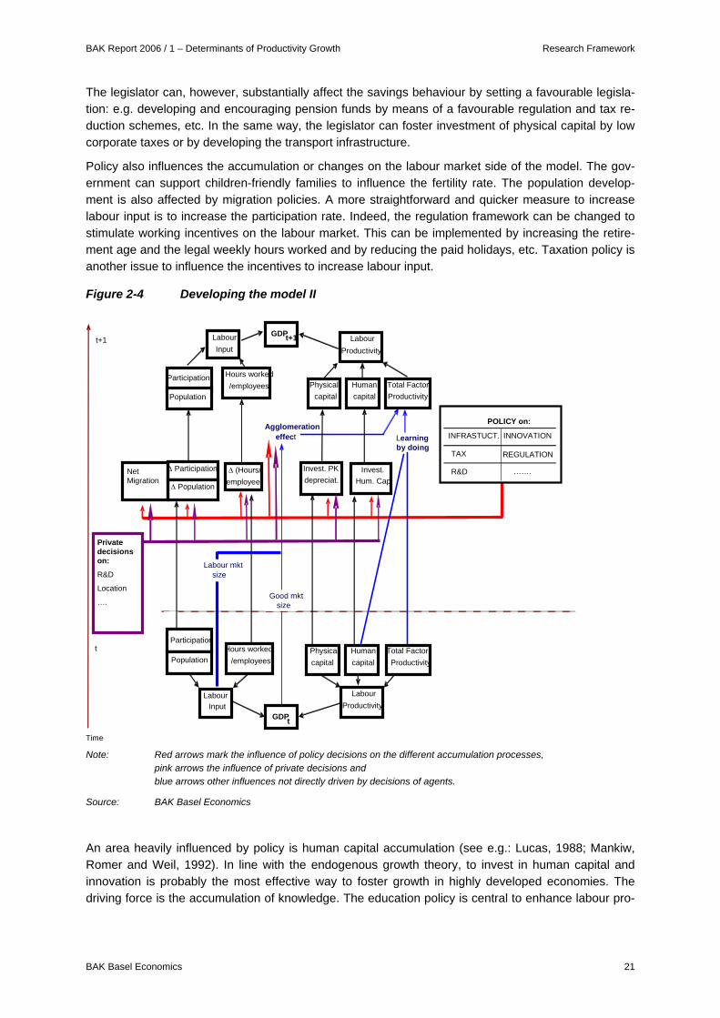
2.3.1 Analytical framework The research is based on a framework of thinking presented in Figure 2-25. As can be seen, policy variables have several separate transmission paths to influence economic performance. Different markets and a variety of accumulation processes play an important role. Thereby, it is not guaranteed that a policy variable influences growth in the same direction through all transmission mechanisms. For example, consider a regulation forcing employees to a certain amount of continuing education. On the one hand, this lowers the labour input available for production and, therefore, influences economic performance negatively. On the other hand, continuing education increases the human capital avail-able. Therefore, productivity increases and economic performance is positively influenced. Theoreti-cally, the direction of the total effect is unknown. Only an empirical investigation can answer the ques-tions about direction and size of the effect of policy variables on economic performance.
5 We are very grateful to the BAK Scientific Advisory Board and especially Prof. Bart van Ark for their input in developing this
framework.

BAK Report 2006 / 1 – Determinants of Productivity Growth Research Framework
BAK Basel Economics 19
The project uses estimations in reduced forms. Therefore, the different transmission mechanisms of a policy can not be evaluated separately6. Only the total effect of a certain policy is at the centre of inter-est. One step in the direction of separating transmission mechanisms is to use individual estimations for productivity growth and labour input changes instead of one estimation with GDP growth as left hand variable. Besides the special interest in productivity in Switzerland, the separation of transmis-sion mechanisms was a reason for choosing this approach. The results presented in this report focus on the effects for productivity growth7.
Figure 2-2 Analytical framework
www.bakbasel.com®
id279
Regionales Benchmarking von BAK Basel Economics: Analyserahmen für nationale und regionale Volkswirtschaften sowie BranchenStand August 2003
Source: IBC Module Determinants 2003Education
expenditure, expenditure für R+D(national, regional)
OECD/CATO Regulation index
(national)
Incicators of interregional and
-Continentalaccessibility
(national, regional)
Taxation of companies and highly skilledmanpower
(national, regional)
Regulation of product markets
Education policies.science policy,
technology policy
Transportation policy,infrastructure policy
Tax and socialpolicies
Regulation of labour markets
OECD/CATO Regulation index
(national)
Labour productivity(Real Gross Value Added
per man hour)
GDP / Gross Value Added
Hours workedper employee
Employeesas % of
resident population
Labour supply(in man hours worked)
Efficiency of factor use(total factorproductivity)
Investment in physical
capital
Investment in intangible
capital
ICT-Capital
Non-ICT-CapitalC
apita
l sto
cksDeterminants
and location
factors
Controlof the
phenomenon
of business
cycles/ dem
and
Monetary
policy
Exchange rate policy
Fiscalpolicy
Externaldemand
(differentiatedby
country, regionor
sector)
Resident population
Population of working age
Demography
Human capital(share of
employees withtertiary
education)
Knowledge capital
(patents and bibliometricindicatros)
Process capital(start-up
companies)
Customercapital
Product markets Capital markets Labour markets
Economic
performance GDP per capita
Source: BAK Basel Economics
This framework of thinking is very helpful in understanding policy influences on growth, but a more formalized model would help to formulate hypotheses to be tested empirically. Based on the thinking outlined in Figure 2-2, the remaining of this chapter will start to develop such a model.
2.3.2 Growth model: based on a production function Most growth models are based on an aggregate production function which asserts a stable relation-ship between aggregate output on the one hand, and labour input, the stock of physical capital, human capital and the state of technology on the other hand. From this perspective, the growth of output de-pends firstly on the growth rate of labour; secondly, on the accumulation of physical and human capi-
6 A complete modelling and estimation of a system of equations would be necessary which is beyond the scope of the project
as well as the power of the dataset as of today. 7 The labour market side will be discussed in a separate report, available probably in summer/autumn 2006.

Research Framework BAK Report 2006 / 1 – Determinants of Productivity Growth
20 BAK Basel Economics
tal, and thirdly, on the speed of technical progress (determining the total factor productivity). Ulti-mately, the determinants of variation of these variables will determine the output growth rate.
Figure 2-3 Developing the model I
Time
GDP t+1
Participation Hours worked/employees
Population
t Physicalcapital
Labour Productivity
Labour Input GDP t
Labour Input
∆ (Hours/employee)
Participation
Population
Hours worked/employees
Human capital
Total FactorProductivity
t+1 Labour Productivity
Physicalcapital
Human capital
Total FactorProductivity
Invest. PK -depreciat.
Invest. Hum. Cap
∆ Participation
∆ PopulationNet Migration
Source: BAK Basel Economics
The model developed here is based on similar relationships. Applying a production function approach, GDP in every period is divided into its elements labour input and labour productivity, and further di-vided into population, employment rate and hours worked on the one side and physical capital, human capital and total factor productivity on the other side. Between two adjoining periods various accumu-lation processes (or ‘change processes’ as they are not necessarily monotonistic) define the level of these variables at the following period which, in turn, define the GDP. Therefore, GDP growth is de-termined by the accumulation processes. Figure 2-3 illustrates this.
2.3.3 Growth model: policy influence In a decentralised market-economy, the interaction between the consumers’ choice (maximisation of utility), the firms’ profit maximisation and the policy makers’ actions will determine the accumulation processes and, finally, the growth path of the economy. For example, the underlying utility preferences (parameters), and the consumer consumption path derived from the intertemporal maximisation prob-lem (Euler equation) will determine the savings rate and, therefore, the level of investment (Ramsey, 1928).
BAK Report 2006 / 1 – Determinants of Productivity Growth Research Framework
BAK Basel Economics 21
The legislator can, however, substantially affect the savings behaviour by setting a favourable legisla-tion: e.g. developing and encouraging pension funds by means of a favourable regulation and tax re-duction schemes, etc. In the same way, the legislator can foster investment of physical capital by low corporate taxes or by developing the transport infrastructure.
Policy also influences the accumulation or changes on the labour market side of the model. The gov-ernment can support children-friendly families to influence the fertility rate. The population develop-ment is also affected by migration policies. A more straightforward and quicker measure to increase labour input is to increase the participation rate. Indeed, the regulation framework can be changed to stimulate working incentives on the labour market. This can be implemented by increasing the retire-ment age and the legal weekly hours worked and by reducing the paid holidays, etc. Taxation policy is another issue to influence the incentives to increase labour input.
Figure 2-4 Developing the model II
INFRASTUCT. INNOVATION
TAX REGULATION
R&D
Time
POLICY on:
GDPt+1
Participation Hours worked/employees
Population
t Physicalcapital
Labour Productivity
Labour Input
GDPt
Labour Input
∆ (Hours/employee)
Participation
PopulationHours worked
/employeesHuman capital
Total FactorProductivity
t+1 Labour Productivity
Physicalcapital
Human capital
Total FactorProductivity
Invest. PK -depreciat.
Invest. Hum. Cap
∆ Participation
∆ Population
Learningby doing
Agglomeration effect
Labour mktsize
Good mktsize
…….Net Migration
Private decisions on:
R&D
Location
….
Note: Red arrows mark the influence of policy decisions on the different accumulation processes, pink arrows the influence of private decisions and blue arrows other influences not directly driven by decisions of agents.
Source: BAK Basel Economics
An area heavily influenced by policy is human capital accumulation (see e.g.: Lucas, 1988; Mankiw, Romer and Weil, 1992). In line with the endogenous growth theory, to invest in human capital and innovation is probably the most effective way to foster growth in highly developed economies. The driving force is the accumulation of knowledge. The education policy is central to enhance labour pro-
Research Framework BAK Report 2006 / 1 – Determinants of Productivity Growth
22 BAK Basel Economics
ductivity. Furthermore, an innovation policy that promotes R&D programs, research in universities, etc., has a direct effect on the rate of technical progress.
But the effect of education and innovation policy is not limited to their direct contribution in the diverse accumulation processes. In many endogenous growth models (see e.g.: Romer, 1990; Grossman and Helpman, 1991; Aghion and Howitt, 1992), the rate of technological change is a function depending on capital (human and physical) and labour. Consequently, all productive factors accumulation generates a positive externality which in turn fosters the speed of technological progress. This further increases the growth rate of output.
Figure 2-4 introduces these effects into the production function approach to explain growth. Policy influences as well as private decisions are schematically included. Although we will at this stage of the research program only estimate reduced forms – the influence of policy variables on (productivity) growth – it is clear from the model that we do not expect policy to influence growth directly, but rather indirectly through a detour through the several accumulation processes. An important implication is that there is no unambiguous mathematical relation between policy and growth in one period, but that policy needs time to affect the accumulation processes and finally growth. And there are no clear theo-retical answers as to how long this ‘time’ might be. Which time lags are appropriate have to be left to the empirical analysis.
Two more issues are included in the model which do not directly link policy and the accumulation processes but are important as well, especially with regard to the external effects of human capital building and innovation policy. First, «learning by doing» refers to the observation that as firms pro-duce goods, they improve the production process and get more efficient over time (Arrow, 1962; Ro-mer, 1986). It can be considered a positive intertemporal spillover effect. Second, as the New Eco-nomic Geography shows, agglomeration does have the potential to increase growth due to economies of scale and positive externalities. The Agglomeration Effect reflects this: a larger market size leads to increased growth, and market size is determined by the production function in the previous period, but can be influenced by political decisions (e.g. market liberalisation) as well.
2.3.4 Growth model: spatial extension The spatial concentration of economic activity is at odds with the traditional comparative advantage and decreasing return to scale hypotheses in the Heckscher-Ohlin-Samuelson framework. Marshall was the first to rationalise this reality by developing agglomeration economics. Agglomeration effects occur if the benefits to clustering are higher than costs.
Beginning with the benefits of agglomeration, we quickly refer back to the discussion of NEG (New Economic Geography). Suppose that the transportation of products involves costs that rise with dis-tance. Concentrating the different production stages close to each other and close to the final market will reduce costs. In other words, production in one geographical region will have increasing returns. The higher the transportation costs are (in relation to total costs) the higher the agglomeration effects are (Ciccone and Hall, 1996). Furthermore, other forces increase the tendency to geographical con-centration. As proved by Krugman (1991) and Venables (1996), in a monopolistic competition frame-work, circular and cumulative causation will strengthen the agglomeration effect by attracting workers and firms to larger markets. Demand linkages (Krugman, 1991) and forward and backward linkages (Krugman and Venables, 1995; Venables, 1996) are the driving forces. Finally, technological spillover between firms drives them to cluster if knowledge and technology is not distributed freely and immedi-ately across space. Baldwin and Ottaviano (1997) prove the clustering forces of knowledge in a model with non-tradable patents. All three effects combined and, over time, drive the agglomeration effect in a self-reinforcing process. In a nutshell, as the market size of intermediate input, output and labour rises, the variety of goods and labour supply increases, improving the production process as well as the products themselves because of more specialisation and diversity.

BAK Report 2006 / 1 – Determinants of Productivity Growth Research Framework
BAK Basel Economics 23
As mentioned above, there are costs as well. We can separate two different kinds of costs. First, the costs which arise in the region in which the concentration takes place due to the fact of higher concen-tration – the agglomeration costs. Second, there are costs for regions which are not at the centre of the development and lose production, firms, labour and consumers.
Turning to the agglomerating regions first, the costs arising from higher concentration are the limiting factor to the concentration. Otherwise, the whole economy would concentrate in one single spot and geography would not matter in an economic analysis. For example congestion costs (traffic jams, crowded transports) are huge and land prices climb to prohibitive levels, worsening firms’ cost. The agglomeration has negative impacts which at a certain level of concentration outweigh the positive spillovers and economies of scale.
As mentioned above, there are costs to other regions as well. The agglomeration effect in region i makes region j worse off especially in a NEG framework. The loss of firms, employment and market size makes production in region j more costly (implied by increasing returns to scale). Even if agglom-eration costs prevent a complete concentration in region i, production in j is less productive and region j is worse off than region i, in absolute terms as well as on a per capita basis. Even if the outcome in a regional growth model is more attenuated in terms of growth rate (indeed the periphery can benefit from the huge crowding activity of the core region), the core-rich and periphery-less developed charac-teristic remains (Baldwin and Martin, 2003). There is clearly an asymmetric outcome in terms of activ-ity location.
The model discussed above8 does not yet include any ‘space’. But as the discussion and the stylised facts show, space plays an important role in the economy and the economic development. We intro-duce space in a way that we focus our interest in the development of one particular region (i). This region has an individual production function with individual levels of inputs and accumulation proc-esses. The infinite number of other regions is subsumed in another region (j) with its own production function and so on. Of course, the accumulation processes in both regions are not independent from one another. Migration does change the labour available in both regions with opposite signs. Knowl-edge transfers can drive the total factor productivity in one region depending on the other regions or advantages of specialisation in both regions in parallel. The interaction between the region of interest and the rest of the world has to be taken into account in the model.
In turn, many of these interactions are politically influenced. For example, consider the case that transport costs are important for a final product and outweigh the advantages of concentrating the production in one region. Firms in both regions will produce the good. For high transport costs, the need to supply markets locally encourages firms to locate to different regions. Suppose that improve-ments of transportation infrastructure would decrease the costs of transport and the advantages of concentration now outweigh the transportation cost. For the whole economy (region i and j) the devel-opment of transport infrastructure is beneficial. However, if we consider the regional units separately, policy advice is more ambiguous. The benefit of developing interregional transport infrastructure for the core region i (where the production would concentrate) is straightforward. For the periphery re-gion j, this is less clear. If both regions are close to each other an improved transport might lead to an integration of region j into the core and therefore foster growth. But if there is no hope to be integrated, the development of transport can be detrimental because it can trigger the departure of the firms from region j without advantages offsetting this.
An important issue is the degree of labour mobility between the regions, as Ottaviano and Thisse (2002) point out. If interregional labour mobility is very low, the lack of interregional mobility severely weakens agglomeration effects and economic activity will remain spatially evenly dispersed. Demand linkages are not at work without labour mobility, and parts of the specialisation gains, namely of spe-
8 See Figure 2-3 and Figure 2-4, Chapter 2.3.2 and Chapter 2.3.3.

Research Framework BAK Report 2006 / 1 – Determinants of Productivity Growth
24 BAK Basel Economics
cialised labour, are also lost. Besides, low interregional labour mobility leads to a wage differential between regions. As shown by Krugman and Venables (1995), for low transport costs some firms relocate from the industrial agglomeration to regions with lower wages. The agglomeration effects are further reduced with low labour mobility. A lower labour interregional mobility is typically observed in Europe, while in the US, labour mobility is higher. Indeed, the regional concentration of economic ac-tivity is much higher in the US compared to Europe.
Figure 2-5 Developing the model III
INFRASTUCT. INNOVATION
TAX REGULATION
R&D
Time
POLICY on:
(relative) ATTRACTIVENESS of Region i
GDPt+1
Participation Hours worked/employees
Population
t Physicalcapital
Labour Productivity
Labour Input
GDPt
Labour Input
∆ (Hours/employee)
Participation
PopulationHours worked/employees
Human capital
Total FactorProductivity
t+1 Labour Productivity
Physicalcapital
Human capital
Total FactorProductivity
Invest. PK -depreciat.
Invest. Hum. Cap
∆ Participation
∆ Population
Learningby doing
Agglomeration effect
Labour mktsize
Good mktsize
…….Net Migration
Private decisions on:
R&D
Location
….
Region j
SpatialSpillovers/ knowledge
Policycompetition
Interregional trade
Interregional labour
migration
Policy ofregion j
Region i
Note: Red arrows mark the influence of policy decisions on the different accumulation processes, pink arrows the influence of private decisions, blue arrows other influences not directly driven by decisions of agents and green arrows the influences originated in other regions.
Source: BAK Basel Economics
Agglomeration effects and concentration also depend on the path of knowledge diffusion. In the case of intraregional technological diffusion (as in the neo-classical model), spatial spillovers are global, and ideas and knowledge circulate easily from region i to region j. The best examples are Chinese regions which copy from Japan and other South East Asia regions, but also from Western firms’ technology. Baldwin and Martin (2003) introduce intertemporal localised technology spillovers. Endogenous growth is consequently geographically concentrated (New Economic Geography). But as technological spillovers are becoming more global (lower barriers to the spatial diffusion), the cost of innovation in region j decreases and so the region starts to innovate and attracts firms. Global knowledge spillovers can make the core-periphery equilibrium unstable and trigger a sudden industrialisation in the periph-ery region, leading to convergence with the core region’s output level. This industrialisation effect is

BAK Report 2006 / 1 – Determinants of Productivity Growth Research Framework
BAK Basel Economics 25
apparent in Slovenia (especially the regions close to Austria and Italy) but also on a wider extent in China, which copies successfully Western technology. Periphery regions are not condemned to re-maining trapped; a voluntary policy to import technology from outside or to innovate itself can trigger an industrialisation and finally lead to convergence.
Now that theory as well as stylised facts provide indications that agglomeration effects are at work but do not lead to final conclusions, the empirical analysis must try to provide such answers. Therefore, we introduce various linkages from the rest of the world to the accumulation processes in the region under investigation in our stylised model. A more detailed modelling would be beyond the scope of the model for the moment, as the empirical analysis is limited as well (reduced forms, data limitations).
2.3.5 Growth model: policy competition In a very optimistic setting, policy variables (regulation, tax, infrastructure, innovation) are considered exogenous. In reality, many observers challenge this view and suggest that «policy competition» is a more realistic setting. For example «tax competition» on corporate income is a recurrent theme during electoral debates. Many politicians, but also economists, fear a «race to the bottom» and propose a «tax harmonisation» scheme at least between EU members (Wilson, 1999). The argument is based on the non-cooperative game Nash equilibrium (prisoner dilemma) which is pareto sub-optimal in terms of welfare. Baldwin and Krugman (2002) cast doubt on this outcome by proving empirically that there is no race to the bottom. According to them, a tax harmonisation could be harmful because catching-up countries would loose an important instrument of policy and convergence would be much more difficult. However, even if there is no «race to the bottom», attracting firms as well as productive labour («war on talents») with all means including tax levels is a common game between regions.
For our model, that means not only do decisions in other regions influence the accumulation proc-esses in the region of interest. It is the relative position of a region with respect to the rest of the world which is – exclusively or additionally – important. Furthermore, political decisions in other regions might therefore also influence the effect of policy decisions in the regions of interest on the accumula-tion processes in the region of interest. It is left to the empirical analysis to tackle this problem further. Not only the indicators for political decisions in the region of interest should be considered, but also the relative position of the region regarding these indicators.
It is worth stressing that the attractiveness of a region is a combination of many factors. For example, a regional policy maker can only invest in R&D by tax revenues, and social welfare provided by the public sector, even when costly, enhances a region’s attractiveness. It is the optimal combination of all policy instruments and taking into account geography, history, initial endowment in capital and labour and the initial state of development, which will make a regional policy successful or not.

Data BAK Report 2006 / 1 – Determinants of Productivity Growth
26 BAK Basel Economics
3 Data Data The data available for the research are taken from the «IBC BAK International Benchmark Club»® database. This database includes indicators of economic performance (Gross Value Added, employ-ment, working volume, productivity, etc.) as well as quantitative measurement of several location fac-tors and framework conditions on the regional level in topics such as innovation, taxation, accessibility, regulation and population. Additional variables to explain regional productivity growth differentials have been constructed using the available data including variables for spatial and industry spillover effects. The following sections contain a brief description of the most important variables used. For a detailed description of the database, please refer to Annex A.
3.1 Variables
3.1.1 Variable to be explained: real productivity growth per man hour At least two sub-models can be derived from the theoretical framework presented above: one to ex-plain demography and labour participation, and the other to explain productivity growth. As a first step of the empirical implementation of the theoretical model, the growth of real productivity per man hour was used as the endogenous variable in this study.
3.1.2 Policy relevant explanatory variables
3.1.2.1 Innovation The IBC database includes a wide range of data on innovation. Unfortunately, as of today, most indi-cators are available for only a relatively small number of regions, especially in the field of «innovation processes» or «innovation output». The results presented here are based on three indicators which are all related to the input of innovation processes. These are the shares of the regional work-force with a secondary and the share with a tertiary education reflecting human capital resources. The third indicator used is the ratio of research and development expenditures to nominal GDP. All three indica-tors are expressed in decimal notation.
3.1.2.2 Taxation Two different kinds of taxation measurement sets are available in the IBC database. The first one is on company taxation. The tax burden on a typical investment is calculated taking all taxes into account. The second set of tax indicators follows a similar concept, but for highly qualified labour. For a given (high) available income, the tax burden is calculated including social security contributions if they do not yield a market equivalent return. Different ’model‘ investments and ’model‘ persons can be used for sensitivity checks. The variables are expressed as tax rates in decimal notation.
3.1.2.3 Accessibility The accessibility of a region is measured by the GDP that can be accessed from the region weighted by travel time. The different travel modes, rail, road and air, are used. The analysis is very detailed; for example, it includes the airport access and check-in times. Two variables are used reflecting intercon-tinental accessibility to destinations outside Europe and interregional accessibility to other regions in Europe respectively. The variables are indexed with 100 for the average.
3.1.2.4 Regulation For regulation we only have data on a country level. Two variables are constructed, reflecting the tightness of regulation of the labour market and the product market respectively. The variables are
BAK Report 2006 / 1 – Determinants of Productivity Growth Data
BAK Basel Economics 27
indexed between 0 and 6, i.e. the higher the number the more regulated a market is. For several years, the OECD Regulation Index can be used as original data. To add variation in the time dimen-sion, OECD time series information on the product market regulation in several industries have been used as well as data from the Frasier Institute (the so called CATO-Indices) to built up a time series for labour market regulation.
3.1.3 Other explanatory variables
3.1.3.1 Population The population in the region is available according to gender and age groups (0-14, 15-64, 65+), measured in 1000 persons. Data is available for the complete observation period and growth rates of population could be used as well. Furthermore, the population density in 1000 persons per square kilometre is calculated.
3.1.3.2 Agglomeration and Spatial Spillover Effects Large urban areas profit from economies of scale due to larger product markets as well as larger la-bour markets. This growth effect is usually called an agglomeration effect. For peripheral regions, the proximity to a metropolitan city can have positive as well as negative consequences. In particular, high-productive workers will move from the peripheral regions into the core of the metropolitan area. For less productive work, the effect can be exactly the opposite: if factor costs in the centre rise, less productive work is outsourced to the periphery. The overall growth effect of larger agglomerations on bordering regions, whose sign is ambiguous ex ante, is called spatial spillover effect. Both for the ag-glomeration and the spatial spillover effect, an indicator was built using population and distance infor-mation.
3.1.3.3 Global and Structural (industry spillover) Effect Regions grow differently due to their unequal industrial composition. The Structural Effect collects the productivity growth impact of different industrial mixes at the beginning of the observation period. It reflects the productivity growth differentials to average western European productivity growth due to the differences in the industrial structure of the economy. The calculation of the structural effect has three stages. In a first step, we calculate a proxy indicator reflecting the productivity which would have been reached if the productivity growth of every industry would have been the western European av-erage growth of the corresponding industry. The regional dimension of this proxy indicator is reached through the use of region specific industry shares in the aggregation process. In a second step, we calculate the difference of step-one-indicator from the actual productivity of the region one year before in percent, so that we get a proxy for a hypothetical productivity growth rate. Finally, this indicator is divided in a structural and a global productivity growth effect by subtraction of the aggregate western European productivity growth (global effect).
3.2 Regional and time period coverage Productivity was basically available for the time period 1980 to 2003, except for the eastern German regions, for which reliable data is only available since 1990. For the period of 1990-2003, the regional coverage contains 220 regions out of 14 countries in Western Europe and the USA (see Figure 3-1).

Data BAK Report 2006 / 1 – Determinants of Productivity Growth
28 BAK Basel Economics
Figure 3-1 Regional coverage
Bassin Lémanique +Ticino
Basel +Zürich
Ostschweiz +ZentralschweizEspace Mittelland
Itä-Suomi
Etelä-Suomi + Aland
Pohj ois-Suomi
Länsi-Suomi
Scotland
Edinburgh
Glasgow
Lorraine
Alsace
Franche-Comté
Varese + ComoPiemonte Nord
Piemonte Sud
Bergamo+
Lombardia SudVerona + Vicenza
Trev iso + Belluno
Padov a + Rov igoVeneziaTorino
MilanoBrescia
Schleswig-Holstein
Hamburg
Niedersachsen
Bremen
BerlinBrandenburg
Mecklenburg-Vorpommern
Sachsen
Sachsen-Anhalt
Thüringen
Schwarzwald-Baar-HeubergNordschwarzwaldRegion Stuttgart
Region KarlsruheFranken / Heibronn
Mannheim / Heidelberg
Reutlingen / UlmSüdost Baden-Württemberg
Unterfranken
Mittelfranken
Schwaben
Oberfranken / Weiden
Ostbayern
Region München
Südostbayern
Mainz
Ludwigshafen / Landau
Baden-Württemberg
Saarland
Übriges Rheinland-Pfalz
Übriges Hessen
Übriges Nordrhein-Westfalen
Københav ns
Danish Islands
Danish Mainland
Var + Vaucluse
Ardèche + Drôme + Loire
Rhône + AinHaute-Sav oie + Sav oie
Alpes de PACA
Isère
Bouches-du-Rhône
Région Wallonne
Vlaams GewestBruxelles / Brussels
Ireland
Luxembourg
Noord-Nederland
Oost-NederlandWest-Nederland
Zuid-Nederland
Ostösterreich
North East
North WestYorkshire And The Humber
East MidlandsWest Midlands
East Of England
South EastSouth West
Wales
Northern Ireland
Île De France
Oslo og Akershus
Trøndelag
Friuli-Venezia GiuliaTrentino-Alto Adige
Liguria
Valle d'Aosta
Cataluña
Comunidad de Madrid
Southern Norge
Kärnten
Steiermark
Oberösterreich
SalzburgTirol
Vestlandet
Rest of Sv erige South
Sv erige Nord
Stockholm
Sydsv erige
Vorarlberg
Nord-Norge
Västsv erige
Köln
Source: BAK Basel Economics
Besides the lack of data for the eastern German regions in the 1980s, some more data limitations showed up with respect to explaining variables. For this reason, unfortunately all US regions, as well as Luxembourg, had to be dropped in the estimation samples. Finally, North-Netherland had to be removed because of large fluctuations in productivity growth. Statistical tests suggested dropping this region for the reason of stability. In the end, the balanced panel sample consisted of 109 regions.

BAK Report 2006 / 1 – Determinants of Productivity Growth Data
BAK Basel Economics 29
Table 3-1 Regional coverage in estimation sample
Source: BAK Basel Economics.
Estimation sample Germany: 29 Sweden: 5France: 21 Netherlands 3Italy: 16 Finland: 4United Kingdom: 13 Belgium: 3Austria: 7 Danmark: 3Switzerland: 7 Spain: 2Norway: 5 Ireland: 1
109
Dropped from overall sample 6 German regions: 10 US-regions: due to missing right hand data Luxembourg: due to missing right hand data1 region from the Netherlands
Eastern German regions
due to outlier with respect to productivity growth
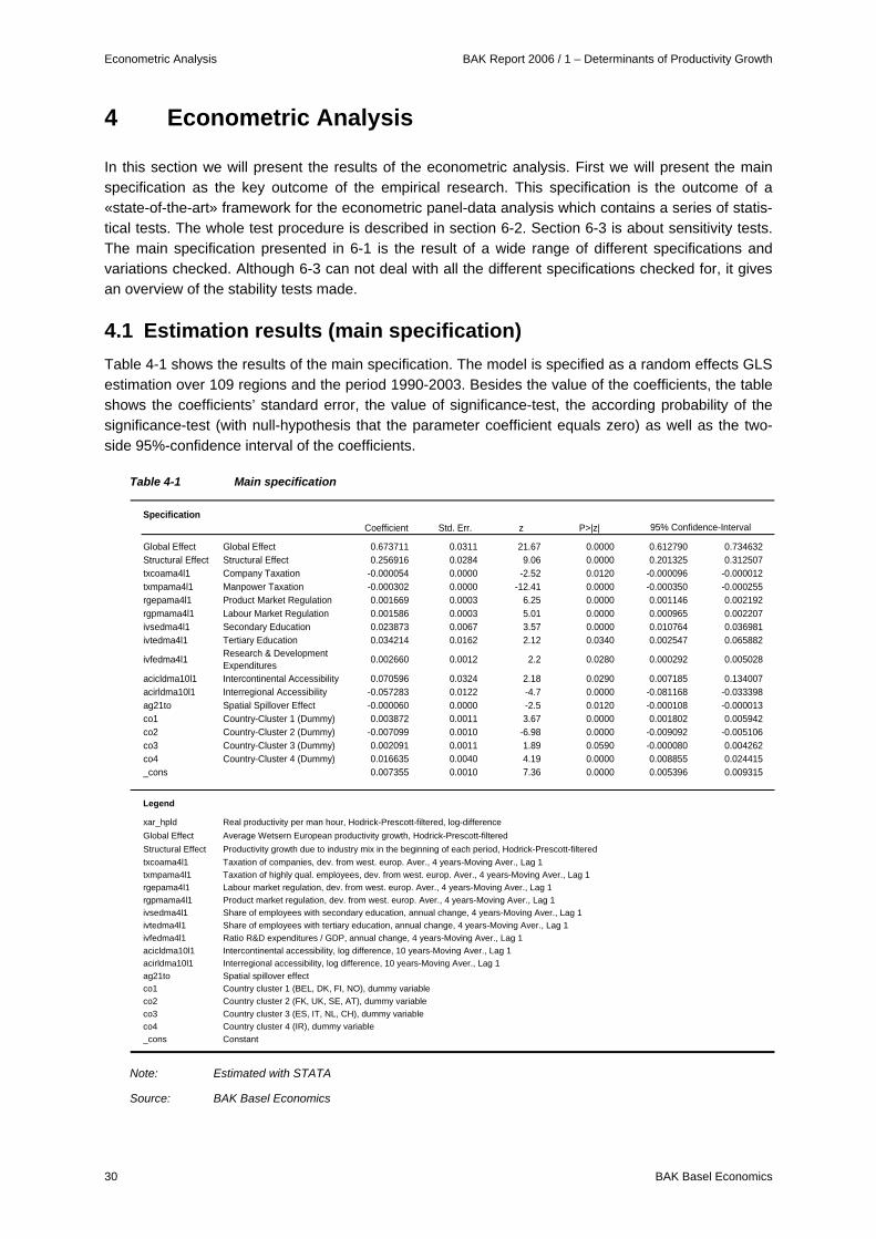
Econometric Analysis BAK Report 2006 / 1 – Determinants of Productivity Growth
30 BAK Basel Economics
4 Econometric Analysis Econometric Analysis In this section we will present the results of the econometric analysis. First we will present the main specification as the key outcome of the empirical research. This specification is the outcome of a «state-of-the-art» framework for the econometric panel-data analysis which contains a series of statis-tical tests. The whole test procedure is described in section 6-2. Section 6-3 is about sensitivity tests. The main specification presented in 6-1 is the result of a wide range of different specifications and variations checked. Although 6-3 can not deal with all the different specifications checked for, it gives an overview of the stability tests made.
4.1 Estimation results (main specification) Table 4-1 shows the results of the main specification. The model is specified as a random effects GLS estimation over 109 regions and the period 1990-2003. Besides the value of the coefficients, the table shows the coefficients’ standard error, the value of significance-test, the according probability of the significance-test (with null-hypothesis that the parameter coefficient equals zero) as well as the two-side 95%-confidence interval of the coefficients.
Table 4-1 Main specification
SpecificationCoefficient Std. Err. z P>|z|
Global Effect Global Effect 0.673711 0.0311 21.67 0.0000 0.612790 0.734632Structural Effect Structural Effect 0.256916 0.0284 9.06 0.0000 0.201325 0.312507txcoama4l1 Company Taxation -0.000054 0.0000 -2.52 0.0120 -0.000096 -0.000012txmpama4l1 Manpower Taxation -0.000302 0.0000 -12.41 0.0000 -0.000350 -0.000255rgepama4l1 Product Market Regulation 0.001669 0.0003 6.25 0.0000 0.001146 0.002192rgpmama4l1 Labour Market Regulation 0.001586 0.0003 5.01 0.0000 0.000965 0.002207ivsedma4l1 Secondary Education 0.023873 0.0067 3.57 0.0000 0.010764 0.036981ivtedma4l1 Tertiary Education 0.034214 0.0162 2.12 0.0340 0.002547 0.065882
ivfedma4l1 Research & Development Expenditures 0.002660 0.0012 2.2 0.0280 0.000292 0.005028
acicldma10l1 Intercontinental Accessibility 0.070596 0.0324 2.18 0.0290 0.007185 0.134007acirldma10l1 Interregional Accessibility -0.057283 0.0122 -4.7 0.0000 -0.081168 -0.033398ag21to Spatial Spillover Effect -0.000060 0.0000 -2.5 0.0120 -0.000108 -0.000013co1 Country-Cluster 1 (Dummy) 0.003872 0.0011 3.67 0.0000 0.001802 0.005942co2 Country-Cluster 2 (Dummy) -0.007099 0.0010 -6.98 0.0000 -0.009092 -0.005106co3 Country-Cluster 3 (Dummy) 0.002091 0.0011 1.89 0.0590 -0.000080 0.004262co4 Country-Cluster 4 (Dummy) 0.016635 0.0040 4.19 0.0000 0.008855 0.024415_cons 0.007355 0.0010 7.36 0.0000 0.005396 0.009315
95% Confidence-Interval
Note: Estimated with STATA
Source: BAK Basel Economics
Legend xar_hpld Real productivity per man hour, Hodrick-Prescott-filtered, log-differenceGlobal Effect Average Wetsern European productivity growth, Hodrick-Prescott-filteredStructural Effect Productivity growth due to industry mix in the beginning of each period, Hodrick-Prescott-filteredtxcoama4l1 Taxation of companies, dev. from west. europ. Aver., 4 years-Moving Aver., Lag 1txmpama4l1 Taxation of highly qual. employees, dev. from west. europ. Aver., 4 years-Moving Aver., Lag 1rgepama4l1 Labour market regulation, dev. from west. europ. Aver., 4 years-Moving Aver., Lag 1rgpmama4l1 Product market regulation, dev. from west. europ. Aver., 4 years-Moving Aver., Lag 1ivsedma4l1 Share of employees with secondary education, annual change, 4 years-Moving Aver., Lag 1ivtedma4l1 Share of employees with tertiary education, annual change, 4 years-Moving Aver., Lag 1ivfedma4l1 Ratio R&D expenditures / GDP, annual change, 4 years-Moving Aver., Lag 1acicldma10l1 Intercontinental accessibility, log difference, 10 years-Moving Aver., Lag 1acirldma10l1 Interregional accessibility, log difference, 10 years-Moving Aver., Lag 1ag21to Spatial spillover effect co1 Country cluster 1 (BEL, DK, FI, NO), dummy variableco2 Country cluster 2 (FK, UK, SE, AT), dummy variableco3 Country cluster 3 (ES, IT, NL, CH), dummy variableco4 Country cluster 4 (IR), dummy variable_cons Constant

BAK Report 2006 / 1 – Determinants of Productivity Growth Econometric Analysis
BAK Basel Economics 31
From a technical point of view, the main results of the regression are:
• All coefficients are significantly different from zero with a confidence-probability of at least 96.8 percent; the vast majority of the coefficients are significant with more than 99 percent.
• Nearly half of the endogenous variables’ variance can be explained. The overall R-squared is 44 percent.
• Coefficient signs are in line with theoretical considerations, except that for product market regula-tion.
• The coefficients of the Global and Structural Effect indicate that a deterministic decomposition within a Shift-Share Analysis overestimates the impact of global developments and industry mix on regional productivity growth9. Nevertheless, these two effects are relevant in the context of regional growth. A global acceleration of annual productivity growth of 1 percentage point leads to a 0.67 percentage point autonomous improvement of the productivity growth of a region regardless of all other influences.
• The coefficient of the Structural Effect is somewhat harder to interpret so that the magnitude of the effect is not obvious from the coefficient only. In Chapter 5, a more illustrative graphical analysis will give some insight concerning this matter. It will be shown that for the regions covered in the sample, the Structural Effect played a quite prominent role during the 1990s.
• For taxation and regulation, the actual level of the variable is less relevant than the relative level compared to the Western European average. Therefore, in these fields of policy, the competition between regions plays an important role.
• Taxation of highly qualified employees shows the strongest impact on productivity growth. A 10%-points decrease of the tax rate differential (to the Western European average) has led to an annual 0.3%-increase in productivity growth during the estimation period 1990-2003.
• The impact of company taxation is significantly negative, too. However, the magnitude of the effect is much lower than for manpower taxation. A 10%-points decrease of the tax rate differential has led to an annual 0.05%-increase in productivity growth during the estimation period 1990-2003.
• Both indicators for regulation show a significant positive impact. A deregulation of labour markets (relative to the Western European average) by one index-unit leads to a fall in annual productivity growth by 0.2 percentage-points. The magnitude of the effect of product market is similar.
• Education has a positive influence on productivity growth. However, the identified impact of human capital resources is quite small. For tertiary education, an increase of the share in the labour force of one percentage point leads to an increase in annual productivity growth of 0.03 percentage points. For the share of people with secondary education, the effect is similar (0.02 percentage points).
• R&D-activity shows a positive impact on productivity growth, too. Although the impact is substantial higher than for the other two innovation variables (secondary and tertiary education), we had ex-pected a much stronger influence. If a region expanded its spending on research and development by one percentage point of GDP, its annual productivity growth increased by 0.2 percentage points.
• Intercontinental accessibility increases efficiency and competitiveness. However, again the impact is smaller than expected. A permanent higher increase of intercontinental accessibility of one per-centage point led to an increase in annual productivity growth of 0.07%.
9 Compare the results from phase I of the research program for a discussion of the deterministic Shift-Share Analysis and
corresponding results.

Econometric Analysis BAK Report 2006 / 1 – Determinants of Productivity Growth
32 BAK Basel Economics
• Interregional accessibility shows a significant influence in the opposite direction, with a coefficient of 0.06. That means: a permanent higher increase of interregional accessibility of one percentage point led on average to an annual decrease in annual productivity growth of 0.06%.
• Peripheral regions suffer from spatial spillover effects. As for the Structural Effect, the coefficient alone does not tell much about the magnitude of the effect and has to be regarded in combination with the actual values of this variable. Again, the reader is referred to Chapter 5. At this point it can be stated that Spillover Effects have been quite important for a number of regions in proximity of large urban areas.
• There is still a substantial, unexplained «national» effect left in the residuals. Therefore, country-dummies have been used to catch these effects. Stability tests showed that grouping countries into four groups are superior to adding one dummy for each country separately. Country cluster 1 con-sists of Belgium, Denmark, Finland and Norway, cluster 2 of France, UK, Sweden and Austria, cluster 3 of Spain, Italy, Netherlands and Switzerland. For Ireland, a separate country-dummy was built (cluster 4). Therefore, the dummies provide information relative to Germany.
• Without country-dummies, the explanatory power of the regression was only about 10 percent. Not yet otherwise explained national effects account for abut 40 percent of regional productivity growth differences.
4.2 Model selection For the selection of the appropriate model, a «state-of-the-art»-framework was used. This framework starts with the problem of variable selection. To account for possible problems with the optimal lag-structure and reciprocal causality, all possible variables are tested on their relationship with productiv-ity growth with a concept known as Granger Causality10. Although Granger Causality does not prove causality in the more common use of the term, it gives some indications on the information content of the series available for estimations.
One weakness of the Granger Causality is that it suggests causality between two series with a strong correlation even if there isn’t any causal relationship, but only a common underlying trend. This prob-lem is addressed with the Panel Unit Root tests, which analyses each series regarding stationarity. A time series is stationary if the underlying characteristics of the data series remain constant across time.
Once we are sure of the stationarity of the variables, we have to set up the appropriate econometric model. The first decision is whether a pooled OLS estimation leads to unbiased estimators or not. If yes, the Pooled OLS is the most efficient model. If not, a further test has to be executed to decide between the Fixed- and the Random Effects model.
10 See Granger (1969)
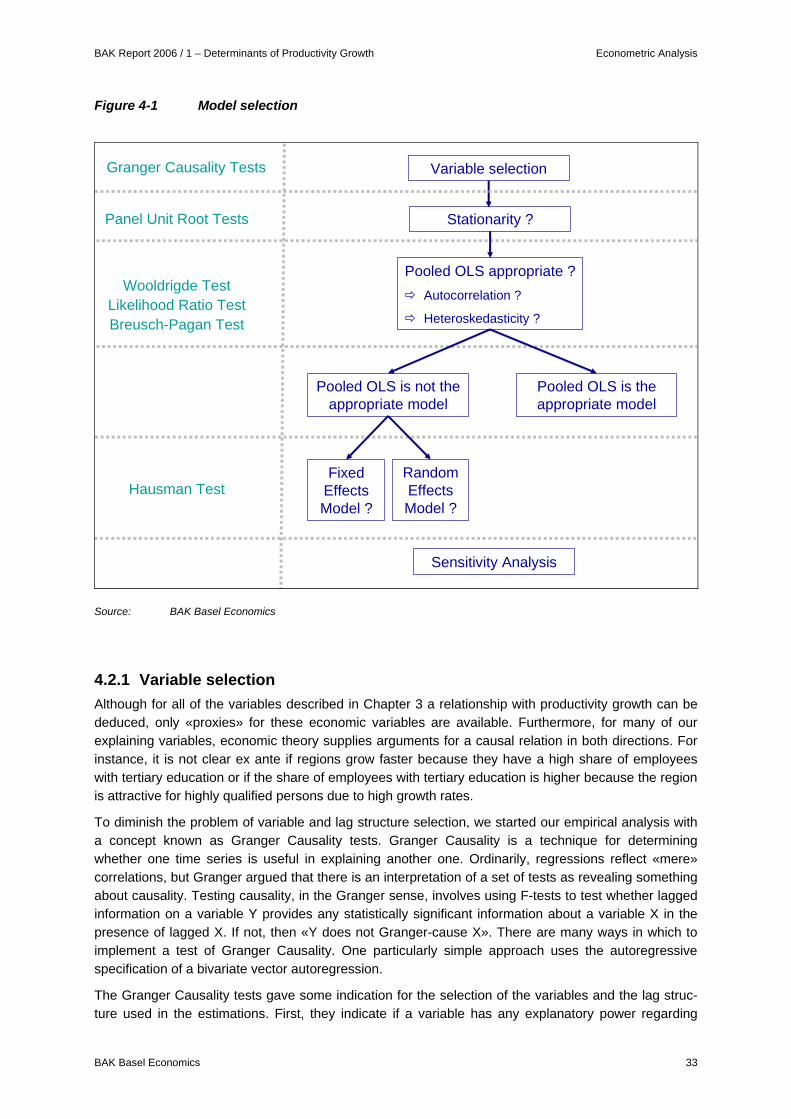
BAK Report 2006 / 1 – Determinants of Productivity Growth Econometric Analysis
BAK Basel Economics 33
Figure 4-1 Model selection
Panel Unit Root Tests
Pooled OLS appropriate ?Autocorrelation ?
Heteroskedasticity ?
Stationarity ?
Wooldrigde TestLikelihood Ratio TestBreusch-Pagan Test
Pooled OLS is not theappropriate model
Pooled OLS is theappropriate model
Hausman TestFixed
EffectsModel ?
RandomEffectsModel ?
Variable selectionGranger Causality Tests
Sensitivity Analysis
Source: BAK Basel Economics
4.2.1 Variable selection Although for all of the variables described in Chapter 3 a relationship with productivity growth can be deduced, only «proxies» for these economic variables are available. Furthermore, for many of our explaining variables, economic theory supplies arguments for a causal relation in both directions. For instance, it is not clear ex ante if regions grow faster because they have a high share of employees with tertiary education or if the share of employees with tertiary education is higher because the region is attractive for highly qualified persons due to high growth rates.
To diminish the problem of variable and lag structure selection, we started our empirical analysis with a concept known as Granger Causality tests. Granger Causality is a technique for determining whether one time series is useful in explaining another one. Ordinarily, regressions reflect «mere» correlations, but Granger argued that there is an interpretation of a set of tests as revealing something about causality. Testing causality, in the Granger sense, involves using F-tests to test whether lagged information on a variable Y provides any statistically significant information about a variable X in the presence of lagged X. If not, then «Y does not Granger-cause X». There are many ways in which to implement a test of Granger Causality. One particularly simple approach uses the autoregressive specification of a bivariate vector autoregression.
The Granger Causality tests gave some indication for the selection of the variables and the lag struc-ture used in the estimations. First, they indicate if a variable has any explanatory power regarding

Econometric Analysis BAK Report 2006 / 1 – Determinants of Productivity Growth
34 BAK Basel Economics
growth at all. Second, Granger Causality tests give some information on the lag structure of the rela-tionship. Third, Granger Causality tests show if there is a bi-causal relationship between location fac-tors and growth. It is important to note that Granger Causality measures precedence and information content but does not by itself indicate causality in the more common use of the term.
Table 4-2 Granger Causality tests I
Granger-Causality between explanatory variables and productivity growth
Number of regions with significant Granger-Causality at 5%-level
Lag=1 Lag=2 Lag=3 Lag=4 Lag=5 Lag=6 Lag=7
txcoa 41 19 9 11 7 9 9
txmpa 73 30 21 21 19 17 6
rgpma 57 34 26 13 15 16 6
rgepa 64 74 48 34 41 37 12
ivsed 6 15 12 8 13 10 7
ivted 7 13 12 7 13 15 4
ivfed 36 13 20 15 12 16 6
acicld 39 16 16 8 10 15 7
acirld 37 27 17 10 12 15 7
Note: Granger-Causality-test only computable up to 7 lags.
Note: Estimated with STATA
Source: BAK Basel Economics
The first series of Granger Causality tests analyses the explaining factors to be considered as having an impact on productivity growth, i.e. the tests examine, if the location variables have any explanatory power with respect to productivity growth. The Granger Causality tests were accomplished with a lag structure from one to seven lags for each variable to be considered. Table 4-2 shows for each test, how many regions (out of a total sample of 110 regions) show significance at the 5%-level in the ac-cording F-test.
Table 4-3 Granger Causality tests II
Granger-Causality between productivity growth and explanatory variables
Number of regions with significant Granger-Causality at 5%-level
Lag=1 Lag=2 Lag=3 Lag=4 Lag=5 Lag=6 Lag=7
txcoa 11 4 2 1 0 0 0
txmpa 8 3 1 0 0 0 0
rgpma 12 1 2 0 0 0 0
rgepa 4 1 0 1 0 0 0
ivsed 13 9 4 2 1 0 0
ivted 22 6 0 0 0 0 0
ivfed 14 3 0 0 0 0 0
acicld 6 3 3 1 0 0 0
acirld 12 2 2 0 0 0 0
Note: Granger-Causality-test only computable up to 7 lags.
Note: Estimated with STATA
Source: BAK Basel Economics
BAK Report 2006 / 1 – Determinants of Productivity Growth Econometric Analysis
BAK Basel Economics 35
As can be seen in Table 4-1, for most of the variables the Granger Causality tests indicate a signifi-cant impact on productivity growth for more than 10 percent of the regions up to a lag-length of six, except that the tests for the two innovation indicators «secondary education» and «tertiary education» indicate a minimum lag-length of two to six.
The second series of Granger Causality tests analyses the reverse causality, i.e. the tests examine if productivity growth has any explanatory power with respect to the location variables. Table 4-3 shows the results as the number of regions with significant F-test at the 5%-level.
For most of the variables, the tests indicate a significant relationship between productivity growth and the location factors in the subsequent period for more than 10 percent of the regions. This can be interpreted as a sign for reverse causality. As the lag-length increases, the number of significant F-tests diminish and disappear with a lag-length of 4 for most of the variables.
The Granger Causality tests show that there is a strong correlation between the explaining variables and productivity growth, that this relationship holds for a number of lags for the location factors and that reverse causality has to be kept in mind seriously at least up to a lag length of two.
4.2.2 Stationarity The concept of stationarity plays an important role in the statistical analysis of economic relationships. In order to get an accurate estimate of the coefficients determining the relationship between two or more variables, the underlying characteristics (mean, variance, contemporaneous covariance) of the data series must remain constant across the sample period. Standard inference procedures do not apply to regressions which contain a non-stationary variable or regressor. Therefore, it is important to check whether the variables considered for estimations are stationary or not before using it in a re-gression.
The formal method to test the stationarity of a series is the Unit Root Test. Recent literature suggests that panel-based Unit Root Tests have higher power than Unit Root Tests based on individual time series. Two different Panel Unit Root tests have been applied in this study, namely the Levin/Lin/Chu-test (LLS) and the Im/Pesaran/Shin-test (IPS)11. Whereas the LLS assumes homogenous autocorrela-tion-coefficients across units, the IPS explicitly allows for heterogeneous autocorrelation-coefficients. For both the LLC and the IPS, we performed the test in three different specifications, with trend and constant, with constant only as well as without both constant and trend. For a detailed description of the concept of stationarity and the corresponding statistical test procedures, please see Annex B.
The Panel Unit Root tests brought up serious problems with respect to the original, non-transformed data. It turned out that most of them are not stationary. For the transformed time series however, non-stationarity turned out not to be a big problem. Table 4-3 shows the result of the Panel Unit Root tests for the transformed variables. For the vast majority of the variables used later on (transformed except the structural effect) stationarity can be stated. This conclusion follows independent of the specifica-tion of the test equation. Nearly all of the transformed variables turned out to be stationary at the 1%-significance level within a test specification without trend and intercept. The specification with constant but without trend still showed stationarity for the vast majority of the tested variables in both test pro-cedures. The specification with both trend and intercept indicated some non-stationarity problems within the LLC-procedure, while the IPS comes to the same conclusions as with the specification with constant only. In the end, we preferred the IPS over the LLC because the LLC does not allow for het-erogeneity across sections (regions).
11 See Levin, Lin and Chu (2002) and Im, Pesaran and Shin (2003)
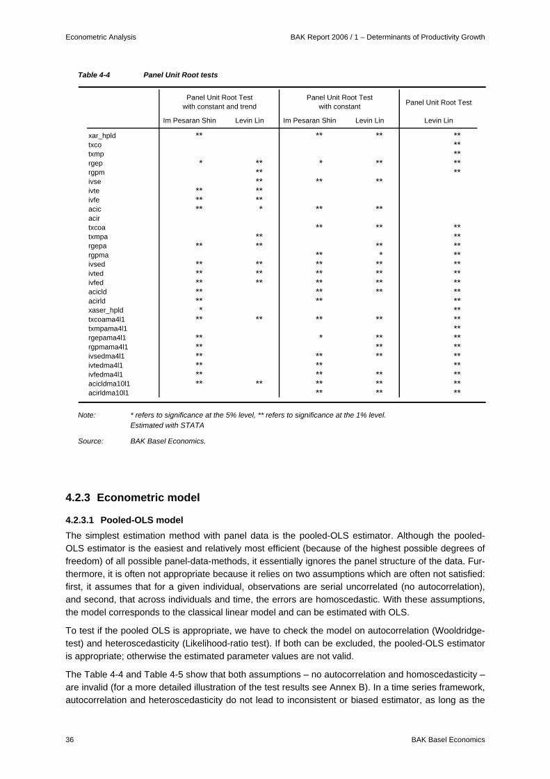
Econometric Analysis BAK Report 2006 / 1 – Determinants of Productivity Growth
36 BAK Basel Economics
Table 4-4 Panel Unit Root tests
Panel Unit Root Test
Im Pesaran Shin Levin Lin Im Pesaran Shin Levin Lin Levin Lin
xar_hpld ** ** ** **txco **txmp **rgep * ** * ** **rgpm ** **ivse ** ** **ivte ** **ivfe ** **acic ** * ** **acirtxcoa ** ** **txmpa ** **rgepa ** ** ** **rgpma ** * **ivsed ** ** ** ** **ivted ** ** ** ** **ivfed ** ** ** ** **acicld ** ** ** **acirld ** ** **xaser_hpld * **txcoama4l1 ** ** ** ** **txmpama4l1 **rgepama4l1 ** * ** **rgpmama4l1 ** ** **ivsedma4l1 ** ** ** **ivtedma4l1 ** ** **ivfedma4l1 ** ** ** **acicldma10l1 ** ** ** ** **acirldma10l1 ** ** **
Panel Unit Root Test with constant and trend
Panel Unit Root Test with constant
Note: * refers to significance at the 5% level, ** refers to significance at the 1% level.
Estimated with STATA
Source: BAK Basel Economics.
4.2.3 Econometric model
4.2.3.1 Pooled-OLS model The simplest estimation method with panel data is the pooled-OLS estimator. Although the pooled-OLS estimator is the easiest and relatively most efficient (because of the highest possible degrees of freedom) of all possible panel-data-methods, it essentially ignores the panel structure of the data. Fur-thermore, it is often not appropriate because it relies on two assumptions which are often not satisfied: first, it assumes that for a given individual, observations are serial uncorrelated (no autocorrelation), and second, that across individuals and time, the errors are homoscedastic. With these assumptions, the model corresponds to the classical linear model and can be estimated with OLS.
To test if the pooled OLS is appropriate, we have to check the model on autocorrelation (Wooldridge-test) and heteroscedasticity (Likelihood-ratio test). If both can be excluded, the pooled-OLS estimator is appropriate; otherwise the estimated parameter values are not valid.
The Table 4-4 and Table 4-5 show that both assumptions – no autocorrelation and homoscedasticity – are invalid (for a more detailed illustration of the test results see Annex B). In a time series framework, autocorrelation and heteroscedasticity do not lead to inconsistent or biased estimator, as long as the

BAK Report 2006 / 1 – Determinants of Productivity Growth Econometric Analysis
BAK Basel Economics 37
errors are orthogonal to the regressors. The only drawback is that making inference is no longer pos-sible (statistical tests are no longer valid). However, in a panel framework, this may indicate the pres-ence of unobserved heterogeneity through individual effects. In that case, the estimated parameters are inconsistent. In conclusion, these results suggest that the OLS estimates suffer from a misspecifi-cation due perhaps to unobserved regional heterogeneity (in which case, we have the problem of omitted variable bias). This problem can be addressed by either adding more explanatory variables or by allowing for additional individual effects in the specification.
Table 4-5 Wooldridge-test
Test for Autocorrerlation
Ho: no first order autocorrelation
Test statistics
Wooldridge test for autocorrelation in panel dataF( 1,108) = 5317.008
Prob(χ2critical > χ2) = 0.0000
Conclusion
first order autocorrelation Note: Estimated with STATA
Source: BAK Basel Economics
Table 4-6 Likelihood-Ratio-test
Test for Heteroskedasticity
Ho: Homoscedasticity
Test statistics
Likelihood-ratio testLR χ2(108)= 943.98
Prob(χ2critical > χ2) = 0.0000
Conclusion no homoscedasticity
Table 4-7 Breusch-Pagan-test
Breusch-Pagan LM-test tests for heteroscedasticity
xar_hpld[unit_n,t] = Xb + u[unit_n] + e[unit_n,t]
Estimated results:
Variance std. deviationxar_hpld 0.0000384 0.0061971e 4.71E-06 0.0021705u 0.0000182 0.0042677
Null-hypothesis: Var(u) =0
Test statisticsχ2 = 4076.27Prob(χ2
critical > χ2) 0.0000
Conclusion individual effects
Note: Estimated with STATA
Source: BAK Basel Economics

Econometric Analysis BAK Report 2006 / 1 – Determinants of Productivity Growth
38 BAK Basel Economics
Another check for individual effects can be done by the Breusch and Pagan12 test that uses a La-grange multiplier test for heteroscedasticity in the error distribution. Again (see Table 4-6), test results suggest the existence of unobserved individual effects.
In conclusion, these results suggest that the OLS estimates suffer from a misspecification due to un-observed regional heterogeneity, which can be addressed by either adding more explanatory variables or by allowing for additional individual effects in the specification.
4.2.3.2 Fixed- versus Random Effects Model The two basic extensions to the simple pooled-OLS model are the fixed- and the random effects model. Both allow for individual effects and can be distinguished in the way this individual effect (in our case region specific effect) is implemented. While the fixed-effects model defines an individual inter-cept, in the random effects model the individual effect it is implemented as a part of the disturbance term. Essentially, the fixed effect model relies on the assumption that the individual effect is correlated with the other exogenous variables, whereas the random-effects model is based on the assumption that the individual effect is uncorrelated with the exogenous variables. For a detailed introduction in these models see Annex B.
Table 4-8 Hausman-test I: model without country-dummies
Hausman Specification TestSpecification without Country-Dummies
Ho: difference in Fixed and Random Effects coefficients not systematic
Fixed Effects Coefficients
Random Effects Coefficients Difference
global_effect 0.675195 0.671552 0.003643structural effect 0.260945 0.274873 -0.013927txcoama4l1 -0.000042 -0.000057 0.000015txmpama4l1 -0.000330 -0.000283 -0.000047rgepama4l1 0.001682 0.001332 0.000350rgpmama4l1 0.001541 0.001153 0.000388ivsedma4l1 0.024111 0.021180 0.002931ivtedma4l1 0.029870 0.040961 -0.011091ivfedma4l1 0.002639 0.002843 -0.000204acicldma10l1 0.056210 0.078021 -0.021811acirldma10l1 -0.055394 -0.056575 0.001181
* Standard error = diag(βFE-βRE)2
Test statistics
χ2(11) = (βFE-βRE)'[(σ2bFE-s2βRE)^(-1)](βFE-βRE) = 164.36
Prob(χ2critical>χ2) = 0.0000
Conclusion Fixed Effects specification is appropriate
Note: Estimated with STATA
Source: BAK Basel Economics
Initially, the Hausman-test13 suggests a Fixed-Effects model for our specification. However, a check of the residuals showed that there is a strong country effect remaining. For this reason, country-dummies
12 See Breusch and Pagan (1979) 13 See Hausman (1978)
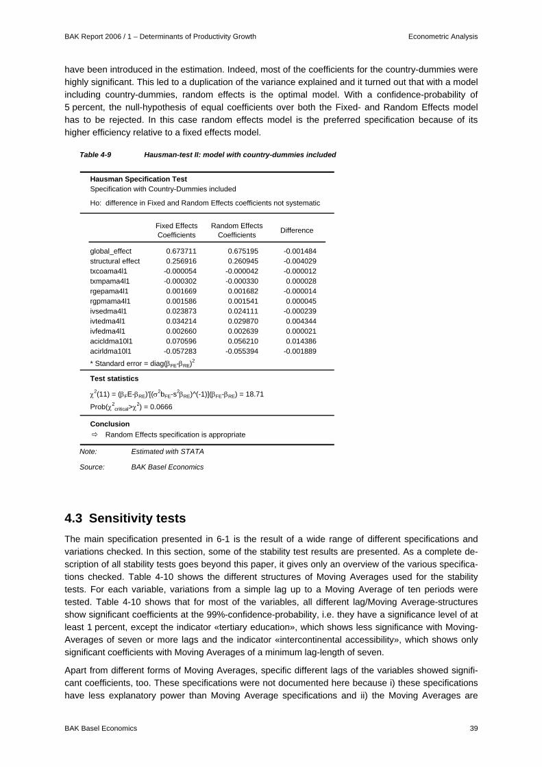
BAK Report 2006 / 1 – Determinants of Productivity Growth Econometric Analysis
BAK Basel Economics 39
have been introduced in the estimation. Indeed, most of the coefficients for the country-dummies were highly significant. This led to a duplication of the variance explained and it turned out that with a model including country-dummies, random effects is the optimal model. With a confidence-probability of 5 percent, the null-hypothesis of equal coefficients over both the Fixed- and Random Effects model has to be rejected. In this case random effects model is the preferred specification because of its higher efficiency relative to a fixed effects model.
Table 4-9 Hausman-test II: model with country-dummies included
Hausman Specification TestSpecification with Country-Dummies included
Ho: difference in Fixed and Random Effects coefficients not systematic
Fixed Effects Coefficients
Random Effects Coefficients Difference
global_effect 0.673711 0.675195 -0.001484structural effect 0.256916 0.260945 -0.004029txcoama4l1 -0.000054 -0.000042 -0.000012txmpama4l1 -0.000302 -0.000330 0.000028rgepama4l1 0.001669 0.001682 -0.000014rgpmama4l1 0.001586 0.001541 0.000045ivsedma4l1 0.023873 0.024111 -0.000239ivtedma4l1 0.034214 0.029870 0.004344ivfedma4l1 0.002660 0.002639 0.000021acicldma10l1 0.070596 0.056210 0.014386acirldma10l1 -0.057283 -0.055394 -0.001889
* Standard error = diag(βFE-βRE)2
Test statistics
χ2(11) = (βFE-βRE)'[(σ2bFE-s2βRE)^(-1)](βFE-βRE) = 18.71
Prob(χ2critical>χ2) = 0.0666
Conclusion Random Effects specification is appropriate
Note: Estimated with STATA
Source: BAK Basel Economics
4.3 Sensitivity tests The main specification presented in 6-1 is the result of a wide range of different specifications and variations checked. In this section, some of the stability test results are presented. As a complete de-scription of all stability tests goes beyond this paper, it gives only an overview of the various specifica-tions checked. Table 4-10 shows the different structures of Moving Averages used for the stability tests. For each variable, variations from a simple lag up to a Moving Average of ten periods were tested. Table 4-10 shows that for most of the variables, all different lag/Moving Average-structures show significant coefficients at the 99%-confidence-probability, i.e. they have a significance level of at least 1 percent, except the indicator «tertiary education», which shows less significance with Moving-Averages of seven or more lags and the indicator «intercontinental accessibility», which shows only significant coefficients with Moving Averages of a minimum lag-length of seven.
Apart from different forms of Moving Averages, specific different lags of the variables showed signifi-cant coefficients, too. These specifications were not documented here because i) these specifications have less explanatory power than Moving Average specifications and ii) the Moving Averages are

Econometric Analysis BAK Report 2006 / 1 – Determinants of Productivity Growth
40 BAK Basel Economics
preferable from a theoretical point of view. Policy measures need time to evolve their impact on real economies performance so the impact of policy measures is expected to be highest when these measures are sustainable (valid over more than one period).
Table 4-10 Parameter stability
?l1 ?ma2l1 ?ma3l1 ?ma4l1 ?ma5l1 ?ma6l1 ?ma7l1 ?ma8l1 ?ma9l1 ?ma10l1
Taxation of companies ** ** ** ** ** ** ** ** ** **
Taxation of highly qualified employees ** ** ** ** ** ** ** ** ** **
Labour market regulation ** ** ** ** ** ** ** ** ** **
Product market regulation ** ** ** ** ** ** ** ** ** **
Share of employees with secondary education ** ** ** ** ** ** ** ** ** **
Share of employees with tertiary education ** ** ** ** ** ** * *
Ratio R&D expenditures / GDP ** ** ** ** ** ** ** ** *
Intercontinental accessibility ** ** ** **
Interregional accessibility * ** ** ** ** ** ** ** ** **
** = significant at 1%** = significant at 5%
Note: Estimated with STATA
Source: BAK Basel Economics
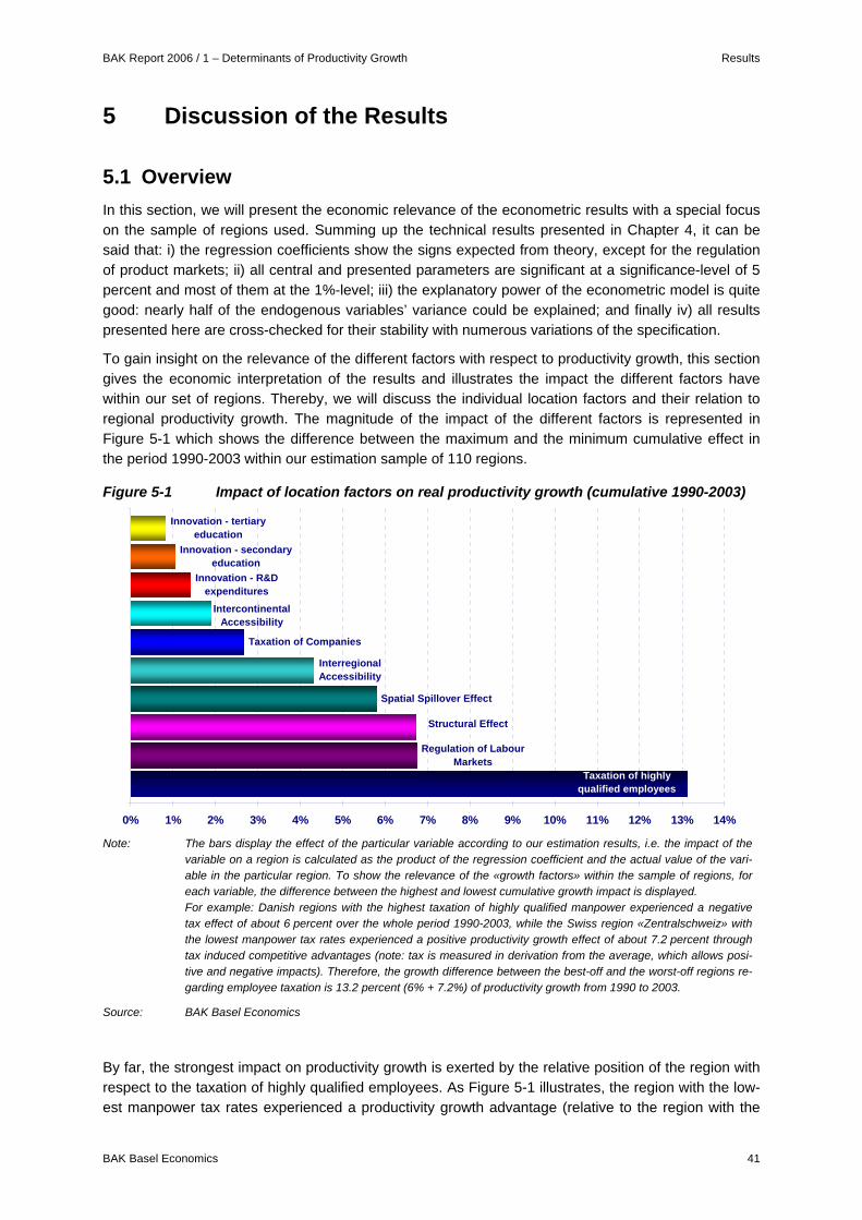
BAK Report 2006 / 1 – Determinants of Productivity Growth Results
BAK Basel Economics 41
5 Discussion of the Results Results
5.1 Overview In this section, we will present the economic relevance of the econometric results with a special focus on the sample of regions used. Summing up the technical results presented in Chapter 4, it can be said that: i) the regression coefficients show the signs expected from theory, except for the regulation of product markets; ii) all central and presented parameters are significant at a significance-level of 5 percent and most of them at the 1%-level; iii) the explanatory power of the econometric model is quite good: nearly half of the endogenous variables’ variance could be explained; and finally iv) all results presented here are cross-checked for their stability with numerous variations of the specification.
To gain insight on the relevance of the different factors with respect to productivity growth, this section gives the economic interpretation of the results and illustrates the impact the different factors have within our set of regions. Thereby, we will discuss the individual location factors and their relation to regional productivity growth. The magnitude of the impact of the different factors is represented in Figure 5-1 which shows the difference between the maximum and the minimum cumulative effect in the period 1990-2003 within our estimation sample of 110 regions.
Figure 5-1 Impact of location factors on real productivity growth (cumulative 1990-2003)
Regulation of Labour Markets
Spatial Spillover Effect
Interregional Accessibility
Taxation of Companies
Innovation - secondary education
Innovation - tertiary education
Taxation of highly qualified employees
Structural Effect
Intercontinental Accessibility
Innovation - R&D expenditures
0% 1% 2% 3% 4% 5% 6% 7% 8% 9% 10% 11% 12% 13% 14%
Note: The bars display the effect of the particular variable according to our estimation results, i.e. the impact of the variable on a region is calculated as the product of the regression coefficient and the actual value of the vari-able in the particular region. To show the relevance of the «growth factors» within the sample of regions, for each variable, the difference between the highest and lowest cumulative growth impact is displayed. For example: Danish regions with the highest taxation of highly qualified manpower experienced a negative tax effect of about 6 percent over the whole period 1990-2003, while the Swiss region «Zentralschweiz» with the lowest manpower tax rates experienced a positive productivity growth effect of about 7.2 percent through tax induced competitive advantages (note: tax is measured in derivation from the average, which allows posi-tive and negative impacts). Therefore, the growth difference between the best-off and the worst-off regions re-garding employee taxation is 13.2 percent (6% + 7.2%) of productivity growth from 1990 to 2003.
Source: BAK Basel Economics
By far, the strongest impact on productivity growth is exerted by the relative position of the region with respect to the taxation of highly qualified employees. As Figure 5-1 illustrates, the region with the low-est manpower tax rates experienced a productivity growth advantage (relative to the region with the

Results BAK Report 2006 / 1 – Determinants of Productivity Growth
42 BAK Basel Economics
highest taxes on highly qualified employees) of over 13 percent during the period 1990-2003. The taxation of companies has a significant influence on productivity growth as well, although its magni-tude – with an impact of about 2.5 percent between the highest and lowest-tax-region – is much smaller than the impact of manpower taxation. This confirms BAK Basel Economics’s earlier research derived by analysing effects on GDP growth. All in all, from the policy indicators available for the re-search, taxation is the field of policy which exerts the most influence on different regional productivity growth experiences and which seems to be the most important issue in the field of productivity growth oriented policy.
The rather small impact of innovation on productivity growth was unexpected, but it has to be inter-preted within the context of data limitations and measurement issues. From another point of view, the results show that innovation is a complex process with many different aspects and that at least not all kinds of innovation policies are quick and easy policy solutions to solve growth problems. Of course, this is by no means proof that innovation orientated policies do not support productivity growth. But it demonstrates that merely focusing on formal secondary or tertiary educational degrees and on pure R&D expenditures without any quality controls might not be an efficient way to foster productivity growth.
In the field of labour market regulation, theory suggests positive as well as negative effects on produc-tivity growth. The empirical analyses reveal a clear dominance of the positive effects. Regions with the tightest labour market system show a growth differential of nearly 7 percent compared to regions with the most liberal system. This result is due to a strong crowding out effect of tight labour market regula-tion on less productive labour. Labour market regulation has a stronger impact on low-skilled people than on highly educated people. Of course, one should not conclude that a tightening of labour market regulation is a promising growth strategy because its impact on productivity is only half of the story. The overall effect of regulation on GDP growth is expected to be negative by all means, because la-bour input – the second component of GDP growth – is expected to be clearly negatively affected by labour market regulation.
Ambiguous results are revealed in the field of infrastructure policy and accessibility. While the im-provement of intercontinental accessibility is aligned with higher productivity growth, this is not the case (for the regions in our sample) with regard to interregional accessibility. For peripheral regions, better accessibility to agglomerations can lead to an outflow of productive resources. The empirical results show that close proximity to an agglomeration leads to «crowding out» of productivity growth.
Apart from policy relevant growth factors, an important influence can be found in the industrial struc-ture of the region. About seven percent of growth differential is determined by the positioning of a re-gion with respect to its industrial mix. Last but not least, it must be stated that there are still country effects which are not explained by the regional policy indicators applied here. National policies, as well as national framework conditions, play a substantial role for a region’s economic performance.
5.2 Innovation Continuous innovation is probably considered the most important factor for steady economic growth in highly developed industrial countries. Although economic theory as well as public discussion by large agree with this statement, the statement alone does not get us very far, neither in explaining regional growth nor when policy decisions are concerned. «Innovation» itself is not something to be measured, nor is it something to be directly targeted by policy. For example, the discussion on Regional Innova-tion Systems shows that innovation is a process strongly related to institutional settings, linked to capi-tal accumulation – especially human capital – and to the development and use of knowledge. As the above discussion shows, it is not one system or process, but rather, there are hundreds, if not thou-sands, of different issues, measures and potential policy actions linked to innovation.

BAK Report 2006 / 1 – Determinants of Productivity Growth Results
BAK Basel Economics 43
Given the above, it is clear that «innovation» itself can not be tested in an econometric setting. In-stead, we tested for the linkage between a variety of variables believed to be related to innovation and economic growth. Of course, the variables to be tested had to fulfil some prerequisites. The variable had to be quantitatively measurable and comparable data had to be available for all regions included in the study. Clearly, there had to be a link between what is thought to be innovation and the variable, proven either by theory and/or by empirical observation. Finally, in a setting aiming at policy decisions, there had to be ways for policy to influence these variables. Given these prerequisites, we ended up with three indicators to be tested in the econometric model.
Two of the variables are linked to human capital. The share of the labour force with secondary educa-tion and the share with tertiary education are two measures for the human capital put to use in the economy. The hypotheses state that higher shares lead c.p. to a higher innovation capacity in the regional economy and, therefore, to stronger economic growth. Of course, the causality in this case is far from obvious. An innovative and fast growing economy is attractive for qualified labour. We used lagged values to shed more light on the direction of the relationship. The test presented above indi-cates the direction flows from human capital toward growth, given the lag structure used in the estima-tions. Furthermore, the use of changes of the share instead of the levels adds confidence to this con-clusion.
The third variable used reflects the resources employed with the explicit goal of innovation. These are the expenditures on research and development. As we have regions of differing sizes in the sample, R&D expenditures are put in relation to the region’s GDP. If R&D resources are rationally spent, higher spending should lead to more innovation and, therefore, to growth. We expect a positive rela-tionship between the economic growth rate and the share of GDP spent on research and develop-ment.
Because we are only explaining productivity, the hypotheses relating innovation to economic growth have to be rechecked regarding their influence on productivity growth. But in the case of innovation, no changes to the hypotheses are necessary – if any, the connection should be stronger. For all the indicators, theory suggests that the impact of the innovation indicators does not change depending on the value of the indicators in other regions. Therefore, we use the values – actually the change of shares – in the region itself and not a deviation from a European average. Furthermore, due to the expected time lag in the effect of changes in the innovation variables, we use the average of the value for a couple of lagged years for any year in which we explain productivity growth (moving average).
The estimations show the expected results: the relation between the innovation indicators and produc-tivity growth are positive. This result is quite stable even when changes are made in the specification. In general, changing the lag structure and the moving average within reasonable boundaries alters the results only slightly. Dropping or adding other variables in the estimation does not lead to substantially different conclusions. If any, the results get insignificant and no conclusion can be drawn.
While the direction of the effect is as expected, the amount of the actual influence on productivity growth is surprisingly small for all three variables. For tertiary education, an increase of the share in the labour force of one percentage point leads to an increase in productivity growth of 0.03 percentage points14. For people with secondary education, a similar increase in the share results in additional pro-ductivity growth of 0.02 percentage points. Finally, if a region expands its spending on research and development by one percentage point of GDP, its productivity growth increases by 0.2 percentage points. Of course, these numbers derived directly from the estimated coefficients are not very informa-tive if the different productivity growth performances of regions are the centre of interest. They have to
14 Please note that here and in the following, the use of lagged variables and moving averages is ignored. The effects dis-
cussed here are in fact equivalent to the aggregated sum of all growth effects in percentage points in later years when all ef-fects of a change in the explanatory variable in one year have been worked through.
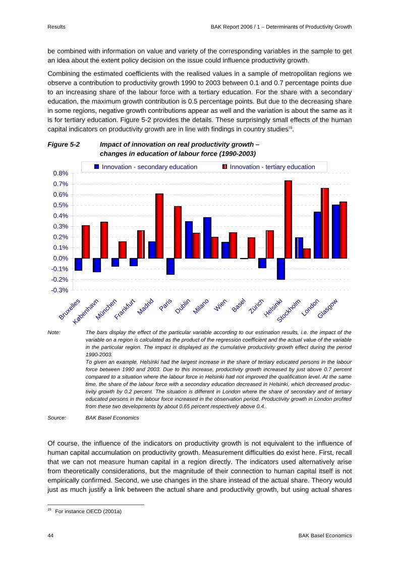
Results BAK Report 2006 / 1 – Determinants of Productivity Growth
44 BAK Basel Economics
be combined with information on value and variety of the corresponding variables in the sample to get an idea about the extent policy decision on the issue could influence productivity growth.
Combining the estimated coefficients with the realised values in a sample of metropolitan regions we observe a contribution to productivity growth 1990 to 2003 between 0.1 and 0.7 percentage points due to an increasing share of the labour force with a tertiary education. For the share with a secondary education, the maximum growth contribution is 0.5 percentage points. But due to the decreasing share in some regions, negative growth contributions appear as well and the variation is about the same as it is for tertiary education. Figure 5-2 provides the details. These surprisingly small effects of the human capital indicators on productivity growth are in line with findings in country studies15.
Figure 5-2 Impact of innovation on real productivity growth – changes in education of labour force (1990-2003)
-0.3%-0.2%-0.1%0.0%0.1%0.2%0.3%0.4%0.5%0.6%0.7%0.8%
Bruxell
es
Københ
avn
Münch
en
Frankfu
rt
Madrid
Paris
Dublin
Milano
WienBas
el
Zürich
Helsink
i
Stockh
olm
Lond
on
Glasgo
w
Innovation - secondary education Innovation - tertiary education
Note: The bars display the effect of the particular variable according to our estimation results, i.e. the impact of the
variable on a region is calculated as the product of the regression coefficient and the actual value of the variable in the particular region. The impact is displayed as the cumulative productivity growth effect during the period 1990-2003. To given an example, Helsinki had the largest increase in the share of tertiary educated persons in the labour force between 1990 and 2003. Due to this increase, productivity growth increased by just above 0.7 percent compared to a situation where the labour force in Helsinki had not improved the qualification level. At the same time, the share of the labour force with a secondary education decreased in Helsinki, which decreased produc-tivity growth by 0.2 percent. The situation is different in London where the share of secondary and of tertiary educated persons in the labour force increased in the observation period. Productivity growth in London profited from these two developments by about 0.65 percent respectively above 0.4..
Source: BAK Basel Economics
Of course, the influence of the indicators on productivity growth is not equivalent to the influence of human capital accumulation on productivity growth. Measurement difficulties do exist here. First, recall that we can not measure human capital in a region directly. The indicators used alternatively arise from theoretically considerations, but the magnitude of their connection to human capital itself is not empirically confirmed. Second, we use changes in the share instead of the actual share. Theory would just as much justify a link between the actual share and productivity growth, but using actual shares
15 For instance OECD (2001a)
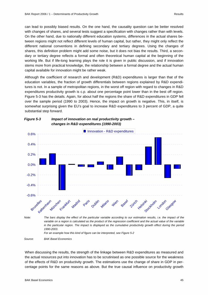
BAK Report 2006 / 1 – Determinants of Productivity Growth Results
BAK Basel Economics 45
can lead to possibly biased results. On the one hand, the causality question can be better resolved with changes of shares, and several tests suggest a specification with changes rather than with levels. On the other hand, due to nationally different education systems, differences in the actual shares be-tween regions might not reflect different levels of human capital, but rather, they might only reflect the different national conventions in defining secondary and tertiary degrees. Using the changes of shares, this definition problem might add some noise, but it does not bias the results. Third, a secon-dary or tertiary degree reflects a formal and often theoretical human capital at the beginning of the working life. But if life-long learning plays the role it is given in public discussion, and if innovation stems more from practical knowledge, the relationship between a formal degree and the actual human capital available for innovation might be rather weak.
Although the coefficient of research and development (R&D) expenditures is larger than that of the education variables, the fraction of growth differentials between regions explained by R&D expendi-tures is not. In a sample of metropolitan regions, in the worst off region with regard to changes in R&D expenditures productivity growth is c.p. about one percentage point lower than in the best off region. Figure 5-3 has the details. Again, for about half the regions the share of R&D expenditures in GDP fell over the sample period (1990 to 2003). Hence, the impact on growth is negative. This, in itself, is somewhat surprising given the EU’s goal to increase R&D expenditures to 3 percent of GDP, a quite substantial step forward.
Figure 5-3 Impact of innovation on real productivity growth – changes in R&D expenditures (1990-2003)
-0.6%
-0.4%
-0.2%
0.0%
0.2%
0.4%
0.6%
Bruxell
es
Københ
avn
Münch
en
Frankfu
rt
Madrid
Paris
Dublin
Milano
WienBas
el
Zürich
Helsink
i
Stockh
olm
Lond
on
Glasgo
w
Innovation - R&D expenditures
Note: The bars display the effect of the particular variable according to our estimation results, i.e. the impact of the
variable on a region is calculated as the product of the regression coefficient and the actual value of the variable in the particular region. The impact is displayed as the cumulative productivity growth effect during the period 1990-2003. For an example how this kind of figure can be interpreted, see Figure 5-2
Source: BAK Basel Economics
When discussing the results, the strength of the linkage between R&D expenditures as measured and the actual resources put into innovation has to be scrutinised as one possible source for the weakness of the effects of R&D on productivity growth. The estimations use the change of share in GDP in per-centage points for the same reasons as above. But the true causal influence on productivity growth
Results BAK Report 2006 / 1 – Determinants of Productivity Growth
46 BAK Basel Economics
might well be the level of the expenditure, not the growth, which would again show a weaker relation-ship when changes are used instead of the share itself. Further, R&D expenditures do not differentiate between private and public sources of funding. While private R&D expenditures are considered profit-able – at least on average – and hence should increase growth, the opinions on public expenditures differ. If public expenditures are less efficient, focused on basic research or are not put to use region-ally – recall the discussion about geographical knowledge spillover which might be less restricted re-gionally due to publication rules – the use of an average of both figures would weaken the results16. Finally, data on R&D expenditures are difficult to measure, especially as time series and on the re-gional level17.
In summary, we do find a positive and stable impact of innovation indicators for human capital and resources put into the innovation process, but their actual effect on productivity growth is rather small. Measurement issues and some technical aspects lead us to the conclusion that we may be underes-timating their effect. Furthermore, the three indicators used here are not sufficient to reflect all issues related to innovation. More emphasis should be put into this kind of research. In particular, more quan-titative, regionally and internationally comparable data is needed on innovation. Still, the results clearly point out that fostering innovation – especially through the broader and less focused areas the indica-tors used here cover – is not the quick and easy policy solution to solve all growth problems. But inno-vation and the indicators used here do have a positive impact on productivity growth. Although the road to travel might be longer than expected, policy supporting innovation is growth policy. The ques-tion could be posed if more focused measures would improve the results as some theoretical consid-erations suggest. But empirical proof that these measures are better suited to supporting growth is still lacking.
5.3 Taxation Taxation is a key topic for businesses when evaluating the attractiveness of a location. In view of in-tensive international competition for capital – and hence for workplaces – the tax burden on compa-nies is one of the most important location factors driven completely by policy. A lower tax burden not only attracts new companies to a location and provides an incentive for existing companies to stay. Given the necessity of a market return on capital, it is also a factor influencing the competitiveness of a firm. A lower tax burden allows ceteris paribus lower prices and, therefore, a potentially higher mar-ket share for the firm. This again is good for local growth. Of course, regions do need taxes to be able to provide infrastructure and public services. But ceteris paribus, if the level of infrastructure and public services is given, lower taxes should increase growth. This is precisely what is tested in the multivari-ate setting used here.
Not only does economic theory suggest such a relationship, but it is also widely accepted in the public discussion. Company taxation, in particular, is thought to be one of the key policy issues to enhance regional attractiveness. Recently, the new EU member countries aggressively followed a low company taxation strategy. But, as the data reveals, they were not the only ones to follow such a strategy. In nearly all the regions in Europe in the sample, the current direct tax burden on companies is lower than it has been on average over the last two decades. Further, it can be observed that the variation of the tax burden between regions has decreased. But direct taxation is not the only tax burden a com-pany has to bear.
Companies have to bear part of the income tax burden of their employees as well. Employees focus on net available income, while firms competing for these employees have to bear the internationally different tax and social security burdens. With the increasing international mobility of labour, especially
16 Unfortunately, no separate figures are available on the regional level at the moment. It is one issue we hope to tackle in the
next phase of this ongoing research project. 17 Quite a bit of the regional data had to be estimated itself. See BAK (2003b).
BAK Report 2006 / 1 – Determinants of Productivity Growth Results
BAK Basel Economics 47
of highly educated employees, and the growing importance of human capital owners in a knowledge based economy, income taxation becomes an ever more important issue in international competition between regions for capital and companies. This suggests that a lower tax burden on highly educated manpower makes a region more attractive for companies and gives companies in the region a com-petitive advantage, just as lower company taxation does. Furthermore, while direct company taxation can, to some extent, be shifted around different locations of a multinational firm together with the prof-its, the tax on manpower is closely tied to the location decision of the company and the workplaces created.
In theory, the relationship between economic growth and taxation is rather obvious, but things are less clear regarding productivity growth. In the case of taxation of highly qualified manpower, a positive connection should be expected as well. Companies employing a large share of highly qualified people are, on average, expected to be more productive. Because international – and even interregional – competition for labour takes place for highly qualified rather than for low skilled labour, the companies whose location decision is influenced by the income tax burden should be the more productive com-panies or company parts. Hence, lower taxation of highly qualified employees should c.p. lead to higher productivity growth. For direct company taxation, this is less straight forward. Still, we would expect a positive connection between company taxation and productivity growth since more produc-tive firms on average have higher profits and, therefore, are more affected by their tax burden.
As for innovation, taxation influences growth through companies’ long term decisions. Therefore, we again use lags and a moving average for the two tax indicators included in the estimation, the average tax burden on a profitable investment of a company and the average tax level on the income of a highly qualified employee. Furthermore, we use derivations of the Western European average instead of the tax level directly. Although the absolute tax level might play some role as well, in the end, it is the tax level compared to competing regions – the “relative tax burden” – which drives development. Control estimations with the tax level directly as well as including changes of the level in the estimation supported this selection and did not lead to any substantially different conclusions.
The estimations show the expected negative influence of the tax levels on productivity growth. Also as expected, the impact of the tax burden on highly qualified manpower is stronger than the impact of direct company taxation. A 10 percentage point higher taxation of highly qualified labour reduces pro-ductivity growth by 3 percent. If direct company taxation is 10 percentage points higher, productivity growth is only reduced by 0.5 percent. These results match quite well the results from the first phase of the «Policy and Regional Growth» project in 200318 which used a far smaller sample and less so-phisticated methods, but had economic growth as its focus. The impact of both kinds of taxes is nega-tive, but income taxation has a stronger effect on growth than company taxation19. As most other stud-ies are not able to discriminate between different kinds of taxes, they can neither support nor contra-dict the finding that manpower taxation is more important for the regional economic development than direct company taxation. But the general negative impact of taxation on economic development is supported by other studies20.
Figure 5-4 gives an even better insight into the importance of taxes for productivity growth than the estimation results alone. For the same set of metropolitan regions as above, the estimation results are combined with the values of the explanatory variables in these regions. We observe that especially the Swiss regions gained from low taxation. About 5 percentage points of productivity growth in Zürich and Basel from 1990 to 2003 are due to their below European average taxation of highly qualified employ-
18 Notice that the research program was called «Regional Growth Factors» at that time. See BAK (2004) and Eichler and Grass
(2004). 19 Due to the limited power of the sample, the estimations in Phase One were inconclusive for company taxation when both
kinds of taxes were included. This fits perfectly with the results presented here based on a more powerful sample even though productivity instead of economic growth is used as the left hand variable and advanced methods are used.
20 Amongst others, Bassanini and Scarpetta (2001), Bleaney, Gemmell and Kneller (2001).
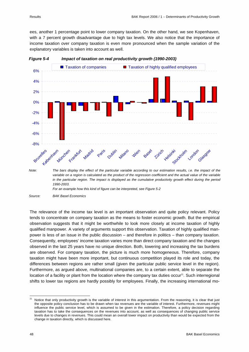
Results BAK Report 2006 / 1 – Determinants of Productivity Growth
48 BAK Basel Economics
ees, another 1 percentage point to lower company taxation. On the other hand, we see Kopenhaven, with a 7 percent growth disadvantage due to high tax levels. We also notice that the importance of income taxation over company taxation is even more pronounced when the sample variation of the explanatory variables is taken into account as well.
Figure 5-4 Impact of taxation on real productivity growth (1990-2003)
-8%
-6%
-4%
-2%
0%
2%
4%
6%
Bruxell
es
Københ
avn
Münch
en
Frankfu
rt
Madrid
Paris
Dublin
Milano
WienBas
el
Zürich
Helsink
i
Stockh
olm
Lond
on
Glasgo
w
Taxation of companies Taxation of highly qualified employees
Note: The bars display the effect of the particular variable according to our estimation results, i.e. the impact of the
variable on a region is calculated as the product of the regression coefficient and the actual value of the variable in the particular region. The impact is displayed as the cumulative productivity growth effect during the period 1990-2003. For an example how this kind of figure can be interpreted, see Figure 5-2
Source: BAK Basel Economics
The relevance of the income tax level is an important observation and quite policy relevant. Policy tends to concentrate on company taxation as the means to foster economic growth. But the empirical observation suggests that it might be worthwhile to look more closely at income taxation of highly qualified manpower. A variety of arguments support this observation. Taxation of highly qualified man-power is less of an issue in the public discussion – and therefore in politics – than company taxation. Consequently, employees’ income taxation varies more than direct company taxation and the changes observed in the last 25 years have no unique direction. Both, lowering and increasing the tax burdens are observed. For company taxation, the picture is much more homogeneous. Therefore, company taxation might have been more important, but continuous competition played its role and today, the differences between regions are rather small (given the particular public service level in the region). Furthermore, as argued above, multinational companies are, to a certain extent, able to separate the location of a facility or plant from the location where the company tax duties occur21. Such interregional shifts to lower tax regions are hardly possibly for employees. Finally, the increasing international mo-
21 Notice that only productivity growth is the variable of interest in this argumentation. From the reasoning, it is clear that just
the opposite policy conclusion has to be drawn when tax revenues are the variable of interest. Furthermore, revenues might influence the public service level, which is assumed to be given in the estimation. Therefore, a policy decision regarding taxation has to take the consequences on the revenues into account, as well as consequences of changing public service levels due to changes in revenues. This could mean an overall lower impact on productivity than would be expected from the change in taxation directly, which is discussed here.
BAK Report 2006 / 1 – Determinants of Productivity Growth Results
BAK Basel Economics 49
bility of labour as well as the growing importance of knowledge in the economy increases the signifi-cance of income taxation levels as location factors.
It should be noted that the special IBC Taxation Module allow a variety of sensitivity tests for the taxa-tion results. For company taxation, we use the effective average tax rate (EATR). The average is rele-vant, for example, in the case of location decision for a company site. We also have information on the effective marginal tax rate (EMTR) available. This indicator is of central interest when deciding the amount to be invested in an existing plant, e.g. to buy another machine22. Using EMTR instead of EATR in the estimations does not lead to substantially different conclusions. For manpower taxation, there are several different indicators available as well. The estimation presented here uses the tax rate on a disposable income of €100’000 for a single person. The IBC Taxation Module also provides in-formation for different income levels, different family status and different incentive packages23. Again, using other indicators does not lead to substantially different conclusions.
In summary, taxation does indeed play an important role in explaining regional growth differentials. In fact, of all the location factors available for research, taxation contributes the most to explain different productivity growth experiences in regions. Interestingly, taxation of manpower has an even greater effect on productivity growth than company taxation does. This econometric result is supported by theoretical considerations and stylised facts. Therefore, it might be time to replace the “old” thinking of company taxation as the trigger to growth and add taxation of highly qualified manpower to the politi-cal growth agenda.
5.4 Regulation Regulation corrects market failures and compensates for externalities. On the other hand, regulation is costly. There are direct costs like administration and controlling, but there are indirect costs as well, e.g. government failure or incompatible incentives with negative consequences for economic growth. From the economic growth perspective, the most important forms of state-run regulation are in the areas of product and labour markets. Since there are costs as well as benefits of regulation, there must be an optimal level of regulation with respect to economic growth which can not be determined theoretically; empirical studies have to be used to answer this question, at least in part.
Although the optimal level is unknown, it is widely believed that in Continental Europe the level of regulation is too high with respect to maximising economic (productivity) growth. Studies based on country data found such an influence. But regulation can differ regionally as well and could explain regional growth differentials. Unfortunately, the data available for this study is on the country level only. Although we are aware of the limitations, we include regulation in the empirical analysis, not least because we are interested in its interaction terms with other variables.
Regulations work through many channels of an economic system, and the relationship between regu-lation and productivity (growth) is very complex. A policy change toward a more liberal system of product markets and higher competition can lead, first of all, to higher efficiency from better resource allocation and more economic use of inputs. While this effect will result in a one-time shift in productiv-ity, higher competition can also lead to higher productivity growth through enhanced efforts to innovate and faster diffusion of innovations.
Liberal labour markets allow the optimal use of the labour force potential. Furthermore, a transition to more flexible labour markets can also lead to faster innovation processes and therefore to dynamic efficiency gains. The implementation of innovations requires the ability to quickly adjust employment to
22 For a more detailed discussion of the different figures and their relevance, see Eichler, Elschner and Overesch (2005) and
Lammersen and Schwager (2005). 23 See Eichler, Elschner and Overesch (2005) and Elschner and Schwager (2005) for more details.
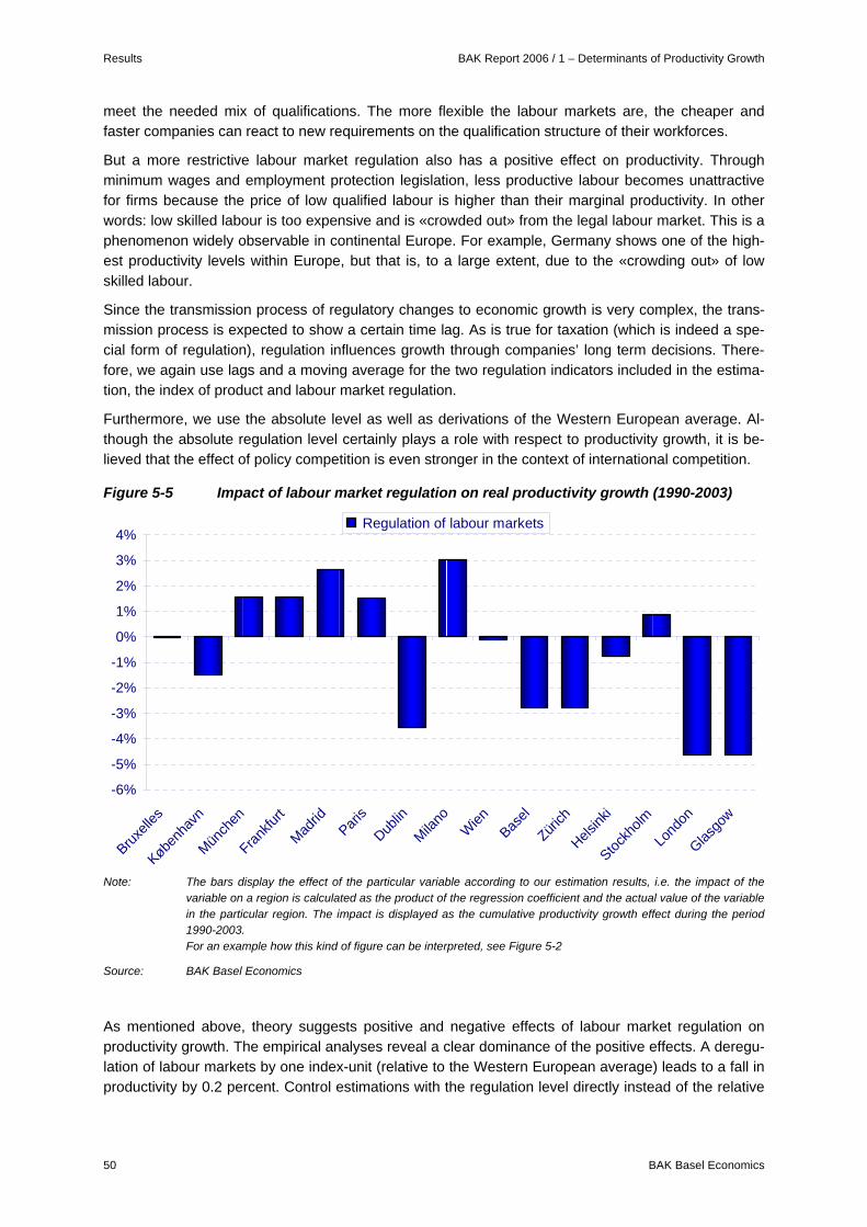
Results BAK Report 2006 / 1 – Determinants of Productivity Growth
50 BAK Basel Economics
meet the needed mix of qualifications. The more flexible the labour markets are, the cheaper and faster companies can react to new requirements on the qualification structure of their workforces.
But a more restrictive labour market regulation also has a positive effect on productivity. Through minimum wages and employment protection legislation, less productive labour becomes unattractive for firms because the price of low qualified labour is higher than their marginal productivity. In other words: low skilled labour is too expensive and is «crowded out» from the legal labour market. This is a phenomenon widely observable in continental Europe. For example, Germany shows one of the high-est productivity levels within Europe, but that is, to a large extent, due to the «crowding out» of low skilled labour.
Since the transmission process of regulatory changes to economic growth is very complex, the trans-mission process is expected to show a certain time lag. As is true for taxation (which is indeed a spe-cial form of regulation), regulation influences growth through companies’ long term decisions. There-fore, we again use lags and a moving average for the two regulation indicators included in the estima-tion, the index of product and labour market regulation.
Furthermore, we use the absolute level as well as derivations of the Western European average. Al-though the absolute regulation level certainly plays a role with respect to productivity growth, it is be-lieved that the effect of policy competition is even stronger in the context of international competition.
Figure 5-5 Impact of labour market regulation on real productivity growth (1990-2003)
-6%
-5%
-4%
-3%
-2%
-1%
0%
1%
2%
3%
4%
Bruxell
es
Københ
avn
Münch
en
Frankfu
rt
Madrid
Paris
Dublin
Milano
WienBas
el
Zürich
Helsink
i
Stockh
olm
Lond
on
Glasgo
w
Regulation of labour markets
Note: The bars display the effect of the particular variable according to our estimation results, i.e. the impact of the
variable on a region is calculated as the product of the regression coefficient and the actual value of the variable in the particular region. The impact is displayed as the cumulative productivity growth effect during the period 1990-2003. For an example how this kind of figure can be interpreted, see Figure 5-2
Source: BAK Basel Economics
As mentioned above, theory suggests positive and negative effects of labour market regulation on productivity growth. The empirical analyses reveal a clear dominance of the positive effects. A deregu-lation of labour markets by one index-unit (relative to the Western European average) leads to a fall in productivity by 0.2 percent. Control estimations with the regulation level directly instead of the relative

BAK Report 2006 / 1 – Determinants of Productivity Growth Results
BAK Basel Economics 51
level did not lead to any substantially different conclusions. However, including changes in the estima-tion led to insignificant parameter coefficients for the level.
According to these results, labour market regulation has a stronger impact on low-skilled people than on the highly educated. First of all, some regulations like minimum wages only affect the less qualified sector of the labour market. Second, the relative burden of regulation in relation to productivity is higher for low-skilled persons. Well-educated employees (with high productivity) participate in the la-bour market regardless of regulation, while low-skilled people (with low productivity) do not get jobs.
Although the empirical results for labour market regulation were stable over various different specifica-tions, they have to be interpreted against the background of the underlying estimation sample. The majority of the regions in the estimation sample (60 out of 110) are from Germany, France and Italy, all countries well known for their high level of employment protection combined with relatively high productivity levels. These three countries are prime examples of the crowding out effect mentioned above.
Of course, one should not conclude that a tightening of labour market regulation is a promising strat-egy for growth because the impact on productivity is only half of the story. The overall effect of regula-tion on GDP growth is expected to be negative by all means because labour input – the second com-ponent of GDP growth – is expected to be clearly affected negatively by labour market regulation. Unfortunately, due to limited resources, the modelling of the labour market could not take place in this project phase. The results for labour market regulation show why the integration of the labour market into the model framework is one of the most important issues on the future research agenda of «Policy and Regional Growth».
Unexpectedly from theoretical considerations and contradictory to various empirical studies with coun-try data24, for product market regulation, the empirical analyses for our set of regions showed a signifi-cant positive influence on productivity growth. Again, this result is mainly driven by our sample. With more than half of the regions from Germany, France and Italy, our sample has a clear focus on coun-tries which experienced a slowdown in productivity growth during the 1990s, while, at the same time, the process of deregulation of product markets was promoted more forcefully in these countries than in many other Western European countries. Consequently, regions from these countries show a sig-nificant improvement in the relative position regarding product market regulation. Due to the fact that other regression variables could not sufficiently explain the slowdown in the productivity growth, the indicator for product market regulation catches this effect through the overweighting of the countries mentioned above. To a large extent, this problem is driven by the fact that we have information on regulation on the country level only. Interregional regulation differences – which certainly do exist – could not be used in the estimation. Having regional data on regulation available would have eased the problem. Further, we suspect that the indicator for product market regulation, which is a variable on the national level only, catches, to some extent, unobserved country effects as well. Due to this line of argumentation, we are not convinced by the empirical results that higher product market regulation has a positive effect on productivity growth. This by no means is proof for the opposite: that lower product market regulation leads to higher productivity growth. Although there are valid theoretical ar-guments for a productivity growth decreasing effect of tighter labour market regulation, its opposite could also be argued for. Again a kind of “crowding out” could be at work, if regulation tends draw “old-styled”, less productive goods and technologies out of the market or forces competitors for companies active in monopolistic markets into new technologies because this is the only way of market access. Although such cases are possible, without much harder empirical evidence, it is hard to believe that this could be the case in the current Western European setting. More research will shed more light on this issue.
24 See for example Nicoletti and Scarpetta (2003), Aghion et al. (2001) and Gust and Marquez (2002).

Results BAK Report 2006 / 1 – Determinants of Productivity Growth
52 BAK Basel Economics
5.5 Accessibility and Agglomeration Effects Accessibility for the workforce of a company to suppliers, customers, or other sources like scientific institutions or even competitors is getting more important. Although well established in theory, it is difficult to evaluate the precise kind of accessibility important for growth. Furthermore, due to a lack of data, only few empirical tests for this hypothesis were possible on the appropriate regional level apart from case studies. For the econometric analysis, we could use two indicators of the accessibility of regions. One is reflecting accessibility on a global scale, using intercontinental travel times. The other reflects accessibility in a European context, based on the travel times between European regions.
In general, good accessibility is thought to be a positive location factor. But as the theoretical discus-sions in the chapters above revealed, that is not necessarily the case. Depending on the characteris-tics of the region and geographical issues, better accessibility can also lead to delocalisation. The following hypotheses are derived:
• Better intercontinental accessibility increases efficiency and competitiveness. Therefore, it should enhance productivity growth.
• For interregional accessibility different effects can lead to either positive (increased efficiency and competitiveness as well as increasing agglomeration gains for central regions) or negative (crowd-ing out, losing high productive employment to more central regions) effects on productivity growth.
• Theory does not show clearly if it is the level of accessibility which influences productivity growth or if changes in accessibility are more important.
• Agglomerations have a productivity advantage (level) due to density and efficiency. Nothing could be said ex ante about the influence of agglomeration on growth of productivity.
• Close proximity to an agglomeration leads to a delocalisation of productivity growth (high produc-tive work is centrally done in the agglomeration; less productive production moves to the periph-ery).
Unfortunately, apart from the more basic problem of how to measure the characteristics of a region, the sample size does not allow us to split the regions up into sub samples with similar characteristics. . Hence, we are not able to clearly discriminate between some of the above hypotheses in the results. But we include two control variables: one reflecting the fact that a region is a central agglomeration, the other one reflecting the proximity to such agglomerations.
Improving accessibility (infrastructure) not only often needs a lot of time, but also quite some time must pass before the effect can be seen in economic variables. Hence, we used a long moving aver-age in the estimation. Apart from levels, we also tried to work with changes. Although some regres-sions showed a significant relationship between the level of accessibility and productivity growth, sta-bility tests proved that it is the change in accessibility in the first place that led to a higher productivity growth in the sample period. Finally, it is important to recognise that all spatial variables are closely related – except possibly intercontinental accessibility. The estimation results for the individual vari-ables can not be interpreted separately, but need to be taken together.
Intercontinental accessibility does have the expected positive effect on productivity growth. Improve-ment in global accessibility in a region leads to higher productivity growth in later years. For example, the Swiss cities, already well connected in 1990, were able to achieve about 0.3 percentage points of productivity growth due to an improvement in global accessibility.
For interregional accessibility, we find a negative – and quite substantial – impact on productivity growth. The delocalisation of highly productive activities in regions when access to more central areas is improved seems to outweigh the positive effects. This might partly be due to an unbalanced effect related to the measurement of accessibility. If a peripheral region and a metropolitan area are con-

BAK Report 2006 / 1 – Determinants of Productivity Growth Results
BAK Basel Economics 53
nected better, the improvement for the first is substantial: not only does it normally have a lower level to start from, but, because accessibility uses GDP-weights, the improvement toward a metropolitan area is also heavily weighted. For the metropolitan area which gains from the delocalisation, the change in accessibility is rather small. This is even more pronounced if connections from the periph-eral region to other destinations in Europe run through the metropolitan region. For the metropolitan region, connections to third destinations will seldom run through the peripheral region. Therefore, the estimation weights the latter effects less. Furthermore, we look at productivity growth and not output growth. While highly productive activity moves to the (few) metropolitan centres, peripheral regions can gain from improved accessibility as well if less productive activities move out of the metropolitan regions due to the high costs there. This hypothesis will be tested within the future research agenda when the influence of location factors on the labour market is empirically analysed as well.
Figure 5-6 Impact of intercontinental accessibility on real productivity growth – changes in intercontinental accessibility (1990-2003)
0.0%
0.1%
0.2%
0.3%
0.4%
0.5%
Bruxell
es
Københ
avn
Münch
en
Frankfu
rt
Madrid
Paris
Dublin
Milano
WienBas
el
Zürich
Helsink
i
Stockh
olm
Lond
on
Glasgo
w
Intercontinental Accessibility
Note: The bars display the effect of the particular variable according to our estimation results, i.e. the impact of the
variable on a region is calculated as the product of the regression coefficient and the actual value of the variable in the particular region. The impact is displayed as the cumulative productivity growth effect during the period 1990-2003. For an example how this kind of figure can be interpreted, see Figure 5-2
Source: BAK Basel Economics
The issue of agglomeration forces and their different impacts on the agglomeration itself and on the peripheral regions around was addressed specifically with two additional variables based on popula-tion and distance data only. Whereas theory implies a positive effect for the agglomeration itself, posi-tive as well as negative effects are conceivable for the surrounding regions from a theoretical view. In our estimations, the latter effect turned out to be negative (and very stable over various different speci-fications). In other words, there are strong regional spillover effects toward agglomerations.
The second variable which, in fact, reflects the agglomeration size of the metropolitan regions showed no significant impact on productivity growth. This indicates that there are no additional agglomeration effects apart from regional spillover effects which work in the direction of large agglomerations. How-ever, it has to be said that more research and a more sophisticated modelling of agglomeration effects have to be done to draw final conclusions on this issue.

Results BAK Report 2006 / 1 – Determinants of Productivity Growth
54 BAK Basel Economics
Figure 5-7 Impact of Spatial Spillover Effects on real productivity growth (1990-2003)
-5%
-4%
-3%
-2%
-1%
0%
East o
f Eng
land
South
East
Restl.
Rheinl
.-Pfal
z
IHK-K
öln
Zuid-N
ederl
and
Région
Wall
onne
Lomba
rdia s
ud
Piemon
te no
rd
Savoie
+ Hau
te-Sav
oieTicin
o
Schwarz
w.-Baa
r-Heu
b.
Sydsv
erige
Danish
Islan
ds
Bassin
Léman
ique+
Stockh
olm
Sverig
e Nord
Spatial Spillover Effect
Note: The bars display the effect of the particular variable according to our estimation results, i.e. the impact of the
variable on a region is calculated as the product of the regression coefficient and the actual value of the variable in the particular region. The impact is displayed as the cumulative productivity growth effect during the period 1990-2003. For an example how this kind of figure can be interpreted, see Figure 5-2
Source: BAK Basel Economics
In summary, the results on spatial and accessibility variables do not yet allow a clear distinction be-tween the different theoretical concepts. The results point to the fact that better accessibility is a dou-ble-edged sword. On the one hand, it enhances business activity and boosts the attractiveness of a region. On the other hand, it allows high value activities to be delivered from a central point. Clearly, more research is necessary before clear-cut policy advice can be given, especially taking different characteristics of regions into account. Also, taking the effects on the labour market side into account is clearly necessary here before policy advice can be formulated.
5.6 Global and Structural (industry spillover) Effect Instead of removing Global and Structural Effects deterministically by a Shift-Share Analysis as in Phase I of the research project, these effects have been taken into account stochastically, i.e. they were introduced into the estimation model as regression variables. The estimation result shows that a deterministic Shift-Share Analysis overestimates the impact of both the global and the structural effect on productivity growth. The coefficients of 0.67 (global effect) and 0.26 (structural effect) are evidence of this (Shift-Share Analysis is basically assuming coefficients of 1). But they also prove that global (here: Western European average) developments as well as global structural trends play a significant role for regional productivity growth.
Although the direct effect of the industrial mix on the regional productivity growth has been imple-mented by the Structural Effect, we did check for the influence more detailed with regressions includ-ing additional industry share variables. There are reasons that there are still significant relationships between the share of an industry in the region and the regional productivity growth. A possible expla-nation is a clustering effect. The industries grow faster in clusters than on average in Western Europe,

BAK Report 2006 / 1 – Determinants of Productivity Growth Results
BAK Basel Economics 55
and an existing cluster leads to a higher share in the region. Other possible explanations include spill-over effects between industries («use of ICT stronger in regions with ICT industries») and unobserved characteristics of the region. However, the regression results did not show clear evidence for these considerations. We found quite significant influence for several industries, but the regressions were not stable over different specifications. Again, more specific research is necessary before clear-cut policy advice is possible.
5.7 Further results As pointed out in Chapter 4, country dummies showed a significant influence on regional productivity growth. These effects can be assigned to national variables not integrated in the estimation. Without country-dummies, the explanatory power of the regression was only about 10 percent, so that national effects not included explicitly in the regression account for abut 40 percent of regional productivity growth differences. Or stated the other way around: about 60 percent of regional productivity growth differences are not determined by national characteristics.

Summary and Conclusions BAK Report 2006 / 1 – Determinants of Productivity Growth
56 BAK Basel Economics
6 Summary and Conclusions Summary and Conclusions Globalisation and decentralisation are challenging the regions’ capacity to adapt and improve their economic competitiveness. It is at the regional level that the pressure to maintain economic growth and social development is felt most. For policy makers, especially for policy makers at the regional level, this leads to the challenge to develop strategies to foster regional growth and therefore eco-nomic well-being in the region. To support decision makers in this challenge and to contribute in an empirically sound way to the ongoing discussion about (location) factors influencing regional growth, BAK Basel Economics, in 2003, started an ongoing research program on «Policy and Regional Growth» within the «IBC BAK International Benchmark Club»®. The second phase of the research program concludes with this study, presenting the results for the influence of a set of regional location factors (or attractiveness factors) on the long term growth of a region. The study selected productivity growth as the dependent variable and as the variables to explain different growth patterns chose indi-cators from the innovation, taxation, regulation and accessibility policy areas plus a number of other indicators such as industrial structure, geography and historical growth rates.
The empirical work relies on the «IBC BAK International Benchmark Club»® and the Club’s unique database. The IBC database is unmatched in Europe in terms of both regional and sector-specific differentiation and data actuality. Currently, it covers up to 400 regions with 64 business sectors per region and annual data from 1980 to 2004. The IBC database is regularly updated and extended. Be-sides indicators of economic performance, the database includes quantitative measures for several location factors and framework conditions as time series, which are, to our knowledge, not available elsewhere in such a rich combination. This dataset allows applying panel methods to a set of regions in an international dimension. Around 120 European regions, with a certain geographical focus on Western Continental Europe, Great Britain and Scandinavia, build the estimation sample. The empiri-cal analysis followed a «state-of-the-art» approach in panel data econometrics which contains a series of test procedures to assure an accurate model specification. The resulting Random Effects model was estimated with Generalized Least Squares for 1990 to 2003. Finally, a sensitivity analysis was performed to guarantee the stability of the results. The econometric results can be summarised as follows:
i) Almost all regression coefficients show the signs expected from theory, i.e. higher taxes reduce productivity growth, more innovation resources increase productivity growth, and better intercontinental accessibility leads to higher productivity growth. For interregional accessibility, the negative effect prevails over the positive effect al-though both are theoretically possible. For productivity growth, central regions crowd out the development of peripheral regions (negative spillover effect), an effect which is increased by better interregional accessibility. Product market regulation does not show the expected sign.
ii) Comparing the individual policy location factors, income taxation of highly qualified employees plays the most important role in explaining productivity growth differen-tials between the regions in our sample. It is followed by regulation of the labour market, interregional accessibility, company taxation, intercontinental accessibility and innovation indicators such as research and development expenditures and edu-cation of the workforce.
iii) Other factors influencing productivity growth in regions are global trends, the indus-trial structure of a region and spatial spillover effects. Large national effects remain as well (captured with country dummies).
iv) All important parameters reported here are significant at a significance-level of at least 5 percent and most of them are at the 1%-level.

BAK Report 2006 / 1 – Determinants of Productivity Growth Summary and Conclusions
BAK Basel Economics 57
v) The explanatory power of the econometric model is quite good; nearly half of the endogenous variables’ variance could be explained (although much of this is due to the inclusion of country dummies).
vi) All results presented here are cross-checked for their stability with numerous varia-tions of the specification.
The results, conclusions and the policy implications for the four policy areas included in empirical tests, namely innovation, taxation, regulation and accessibility, are discussed below individually and in some more detail.
Innovation:
Regionally available innovation resources positively influence productivity growth in the re-gion. All three available indicators (research and development expenditures as share of GDP, the share of the labour force with a secondary and the share with a tertiary degree) do have positive, significant and stable coefficients. But, somewhat surprisingly, the impact the innovation indicators exhibit on productivity growth is low. Different reasons could lead to such a finding in our setting, even if innovation itself is more important for productivity growth. This includes, first of all, the available choice of indicators which were mainly based on the qualification of the workforce. Formal qualification, for instance, need not necessarily reflect actual capacity to do complex jobs or the ability to react quickly to market demand. However, the results confirm the finding of other studies (OECD, 2001a) that secondary education is at least as important as tertiary education and that «learning by doing» and «learning on the job» are as important as academic titles and diplomas. The strongest influence is exerted by research and development which confirms the policy implications of the new regional growth theory and the alleged effects of a strong localised knowledge base. The three indicators used here are not sufficient to reflect all issues related to innovation. More emphasis should be put into this kind of research. In particular, more quantitative, regional and international comparable data is needed on innovation.
Policy with respect to innovation might thus take different directions: the results clearly point out that fostering innovation is not the quick and easy policy solution to solve all growth prob-lems, especially if the policy concentrates on the broader and less focused areas of innova-tion resources which are covered by the indicators available here. Although innovation does have a positive impact on productivity growth, the road there might be longer than expected. It has been shown that while highly qualified labour is important, education at the secondary level («Berufsbildung») should not be neglected. Research and development to increase in-novative capacity is a crucial means to increase regional competitiveness, but especially for public spending on R&D, quality and efficiency controls are necessary. Rather than drowning in the micromanagement of innovative firms, clusters and R&D expenditures, innovation pol-icy should again put more weight on the general framework conditions such as the regulatory burden and its impact on the ability of an economy to innovate. Also, knowledge and tech-nology transfer to firms from universities and other research and education institutions are as important as the creation of knowledge itself. While public money might be a crucial factor for having a better qualified workforce and more knowledge transfer, introducing more market incentives into the innovation process could also improve its effectiveness with respect to economic growth.
Summary and Conclusions BAK Report 2006 / 1 – Determinants of Productivity Growth
58 BAK Basel Economics
Taxation:
The two indicators for taxation, the tax burden on investments and the tax burden on highly qualified employees, both influence productivity growth negatively. It is noteworthy that the impact shows a considerable time lag and that the relative position with regard to other re-gions turns out to be more important than the absolute level of taxation. The indicator «taxa-tion of highly qualified employees» has by far the strongest impact on long term productivity growth of all the indicators included in the estimations. The impact is much stronger than the impact of company taxation.
These findings have two policy implications. First, fiscal policy is indeed an important attrac-tiveness factor. Individuals and the firms that hire them have a strong tendency to choose low-tax locations. Regions may thus, within the scope of national tax law, use their local fiscal policy as a tool for long term development. Second, the tax burden on individuals has a much stronger impact on productivity growth than the tax burden on firms. This is compatible with the hypothesis that competition for capital assets (firms) has been so fierce in the past and has reduced tax rates on firms so much that the latter no longer have a distinctive role for a firms’ location choice (given the individual level of public services). Corporate tax rates all over Europe appear to have reached a rather uniform and low level. Indeed, fiscal competi-tion appears to have shifted away from capital toward labour which, in the last one or two decades, has become ever more mobile. Whereas 20 years ago regions and countries com-peted for mobile firms, they now compete for their highly qualified mobile staff. Taxation of individuals finally affects the number and the size of firms willing to settle in a region, espe-cially if they need a large share of highly qualified labour. Typically, these are the firms driv-ing productivity growth – for the labour market input in GDP growth, the results can differ or at least be less pronounced. After tax reforms that mainly concerned company taxation, re-gions should now presumably turn their attention to the taxation of individuals, especially of those with high skills, if they want to increase their well-being (and tax income) and to with-stand increasing international tax competition.
Regulation:
Labour market regulation has a strong positive impact on productivity growth. Tighter regula-tion can indeed increase the productivity of the working population, but at the price of reduc-ing the participation of the population in the working process. Many regulations like minimum wages affect only less qualified labour. Furthermore, regulation has a higher weight in the la-bour costs of less productive workers than for more productive workers. Well-educated em-ployees (with high productivity) participate in the labour market regardless of regulation, while low-skilled people (with low productivity) do not get jobs. In the long run, labour market regu-lations often hurt most those whom they pretend to protect.
Of course, one should not conclude that a tightening of labour market regulation is a promis-ing strategy for growth because its impact on productivity is only half of the story. The overall effect of regulation on GDP growth is expected to be negative by all means, because labour input – the second component of GDP growth – is expected to be clearly affected negatively from labour market regulation. Furthermore, tight labour market regulation may exclude a part of the population form the labour market and may thus counteract the general objective of social integration. Moreover, low participation may threaten the financial balance of social security systems. Policy measures that focus uniquely on productivity growth without taking into account their impact on other GDP components could in the end lead to lower GDP growth rates. Given that all parts of the population should participate in social well-being,

BAK Report 2006 / 1 – Determinants of Productivity Growth Summary and Conclusions
BAK Basel Economics 59
easy access to the labour market is probably the best policy strategy to enable long term growth and social inclusion.
No conclusion can be drawn for product market regulation. Contrary to the hypotheses as well as to empirical studies with country data, product market regulation shows a positive in-fluence on productivity growth. This result is less stable than the ones presented above – in different specifications the coefficient is insignificant – and we have reason to believe that this is a statistical artefact related to the problem that information on regulation is not avail-able at the regional level and we had to rely on national data. These, in turn, are highly af-fected by EU driven liberalisation in a common way. Still, the results shed some doubt on the importance of deregulation of product markets for productivity growth. Again, the story can be different for GDP growth, which will be analysed in the next step of the research program.
Accessibility:
Interestingly, the two indicators for intercontinental and interregional accessibility yield oppo-site results. While intercontinental accessibility has a positive impact on productivity growth, interregional accessibility – which includes not only air but also land transport – has a surpris-ing negative effect. This might be a statistical effect: accessibility in rural and remote areas increased, with the help of EU Structural Funds, much more than in metropolitan areas, al-though the economic growth of the latter was higher. But there is also a «real» economic ef-fect behind this. Specialists in transport economics have often pointed out that improving in-frastructure between remote and metropolitan areas may benefit the latter more than the former. Transport policies with the objective of bettering the connection between urban and remote areas could thus have the unexpected result of actually reducing the growth potential of remote regions. The reason for this could be a delocalisation effect, i.e. the out migration of highly productive industries toward the economic centres of a country, from where the rural population can then be better served. Growth-inspired transport and infrastructure policy probably benefits mostly urban areas, while for the more rural areas, it may end in disap-pointment. Better accessibility is a double-edged sword. On the one hand, it enhances busi-ness activity and boosts the attractiveness of a region. On the other hand, it allows high value activities to be delivered from a central region. For productivity growth, the latter effect predominates. Again, for GDP growth the conclusions could be different as low value added activities move to the periphery with better transportation to serve the metropolitan area cheaper.
The empirical results presented in this study – the evaluation of the influence of various location fac-tors and other variables on productivity growth in a sample of European regions – lead us to a few clear-cut policy conclusions:
i) Fiscal policy should be a key element in a regions’ growth strategy. After tax reforms that mainly concerned company taxation, regions should not forget to turn their at-tention to the taxation of highly qualified individuals as well.
ii) Innovation policy supports growth, but not just any kind of innovation policy is the quick and easy policy solution to growth problems. Quality and efficiency controls are important.
iii) The attractiveness of a region for highly qualified labour is becoming an ever more important part of fostering growth in highly developed knowledge economies. Taxa-tion of individuals is one issue, but there are various other policy areas to increase the regional attractiveness for such individuals.

Summary and Conclusions BAK Report 2006 / 1 – Determinants of Productivity Growth
60 BAK Basel Economics
iv) Policy takes time. The lag structure of the variables suggests that the effect of a specific policy exceeds the election period of politicians. Especially in cases where policy decisions are unpopular, the future positive effects will have to be clearly ex-plained and communicated to stakeholders and to the population.
v) Regions are not self-contained and the economic development of a region might be influenced by political decisions in other regions. «Policy competition» is a realistic setting. It is often the relative position of a region with respect to the rest of the world which is – exclusively or additionally – important for economic development.
vi) It is worth stressing that the attractiveness of a region is a combination of many fac-tors. It is the optimal combination of all policy instruments taking into account geog-raphy, history, initial endowment in capital and labour and the initial state of devel-opment, which will make a regional policy successful or not.
Although global and structural factors beyond the reach of policy play an important role, long term growth and development are not destiny, but can be influenced by political framework conditions and wise policy decisions. Put in other words: policy matters for regional growth, a region’s policy matters as well as the national one.
This study has focused on productivity growth of a set of European regions, trying to link growth rates to a number of attractiveness factors – or location factors – such as innovative capacity, tax rates, accessibility and the regulatory environment. The study is part of an ongoing research project of BAK Basel Economics to contribute to the discussion on drivers of economic growth. This leaves various options to continue the research. In the next project phase, the major extensions planned are:
i) Model extension: Integration of the labour market as a complement «module» to productivity particularly in order to gauge the effect of different policy measures on productivity and participation of the workforce. Combining both results will also allow conclusions for the drivers of GDP growth, which is indeed the most interesting vari-able. But a separation in labour and productivity allows a more in-depth understand-ing of the underlying mechanisms.
ii) Geographical extension: Inclusion of additional regions, particularly US-American regions with different institutional backgrounds. This should increase the reliability of the results and make comparisons between Europe and the United States – or be-tween their different underlying economic systems – possible. Furthermore, more variety in the dataset and degrees of freedom allow more complex model specifica-tions.
iii) Data extension: More explaining variables (especially indicators on innovation proc-esses and outcomes) to enhance the specification of the model.
iv) Industry specific analysis, i.e. analysis of the impact of location factors on specific industries and business sectors.

BAK Report 2006 / 1 – Determinants of Productivity Growth Reference
BAK Basel Economics 61
7 Reference Reference Reference Ahmed, H. and S. Miller (1999):
«The Level of Development and the Determinants of Productivity Growth», Working Papers 1999-03, University of Connecticut, Department of Economics.
Aghion, P. and P. Howitt (1992):
«A Model of Growth through Creative Destruction», Econometrica, 60(2), pp. 323-351. Aghion, P., C. Harris, P. Howitt and J. Vickers (2001):
«Competition, Imitation and Growth with Step-by-Step Innovation», Review of Economic Studies, 68(3), pp. 467-492.
Arrow, K. (1962):
«The Economic Implication of Learning by Doing», Review of Economic Studies, 29(3), pp.155-173. BAK (2003a):
«IBC Report 2003 Volume I: Papers», Basel: BAK Basel Economics research report, www.bakbasel.com.
BAK (2003b):
«MONITORING INNOVATION IN REGIONS: Schlussbericht Phase 2», Basel: BAK Basel Econom-ics research report, www.bakbasel.com.
BAK (2004):
«IBC Report 2004», Basel: BAK Basel Economics research report, www.bakbasel.com. BAK (2005a):
«IBC Report 2005», Basel: BAK Basel Economics research report, www.bakbasel.com. Baldwin, R. and G. Ottaviano (1997):
«Multiproduct Multinationals and Reciprocal FDI Dumping», CEPR Discussion Paper, No. 1851. Baldwin, R. and P. Krugman (2002):
«Agglomeration, Integration and Tax Harmonization», NBER Working Paper, No. 9290. Baldwin, R. and P. Martin (2003):
«Agglomeration and Regional Growth», CEPR Discussion Paper, No. 3960. Barro, R. (1998):
«Determinants of Economic Growth: A Cross-Country Empirical Study», Cambridge: MIT Press. Barro, R. and J-W. Lee (1993):
«An International Comparison of Educational Attainment», Journal of Monetary Economics, 32(3), pp. 363-394.
Barro, R. and X. Sala-i-Martin (1991):
«Convergence across States and Regions», Brookings Papers on Economic Activity, 1991(1), pp. 107-182.
Barro, R. and X. Sala-i-Martin (1992):
«Regional Growth and Migration: A Japan-U.S. Comparison», NBER Working Paper, No. 4038. Bassanini, A. and S. Scarpetta (2001):
«The driving forces of economic growth: panel data evidence for the OECD countries», OECD Eco-nomic Studies No. 33 (2001/II), Paris: OECD, pp. 9-56.

Reference BAK Report 2006 / 1 – Determinants of Productivity Growth
62 BAK Basel Economics
Blanchard, O. and L. Katz (1992): «Regional Evolutions», Brookings Papers on Economic Activity, 1992(1), pp. 1-75.
Bleaney M., N. Gemmell and R. Kneller (2001) :
«Testing the Endogenous Growth Model: Public Expenditure, Taxation and Growth over the Long-run», Canadian Journal of Economics, 34(1), pp. 36-57.
Braczyk, H., P. Cooke and M. Heidenreich (1998):
«Regional Innovation Systems: The Role of Governances in a Globalized World», London: UCL Press.
Brakman, S., H. Garrestsen and M. Schramm (2002):
«New Economic Geography in Germany: Testing the Helpman-Hanson Model», Hamburgisches Welt-Wirtschafts-Archiv (HWWA), HWWA Discussion Paper, No. 172.
Brakman, S., H. Garrestsen and M. Schramm (2004):
«Putting New Economic Geography to the Test: Free-ness of Trade and Agglomeration in the EU Regions», Paper prepared for the HWWA conference on «New Economic Geography – Closing the Gap between Theory and Empirics», October 2004, Hamburg.
Breusch, T. and A. Pagan (1979):
«A Simple Test for Heteroscedasticity and Random Coefficient Variation», Econometrica, 47(5), pp. 1287-1294.
Cass, D. (1965):
«Optimum Growth in an Aggregative Model of Capital Accumulation», The Review of Economic Studies, 32(3), pp. 233-240.
Ciccone, A. and R. Hall (1996):
«Productivity and the Density of Economic Activity», American Economic Review, 86(1), pp. 54-70. Cooke, P. (1992):
«Regional Innovation Systems: competitive regulation in the new Europe», Geoforum, 23(3), pp. 365-382.
Cooke,.P. (1998):
«Introduction: origins of the concept», in H. Braczyk, P. Cooke and M. Heidenreich (eds): «Regional Innovation Systems: The Role of Governances in a Globalized World», London: UCL Press, pp. 2-25.
Cooke, P. (2001):
«Regional Innovation Systems, clusters, and the knowledge economy», Industrial and Corporate Change, 10(4), pp. 945-974.
Davis, D. and D. Weinstein (1998):
«Market access, economic geography and comparative advantage: an empirical assessment», NBER Working Paper, No. 6787.
De la Fuente, A. (2002a):
«Convergence across Countries and Regions: Theory and Empirics», EIB Papers, 5(2), pp. 25-46. De la Fuente, A. (2002b):
«The Effect of Structural Fund Spending on the Spanish Regions: An Assessment of the 1994-99 Objective 1 CSF», CEPR Discussion Paper, No. 3673.
De la Fuente, A. (2003):
«Does Cohesion Policy Work? Some General Considerations and Evidence from Spain», Working paper prepared for a conference on income convergence and European regional policy organized by the Bertelsmann Foundation, the World Bank and Fundación CIDOB.

BAK Report 2006 / 1 – Determinants of Productivity Growth Reference
BAK Basel Economics 63
De la Fuente, A. and R. Doménech (2002): «Human Capital in Growth Regressions: How much Difference does Data Quality make? An Update and Further Results», CEPR Discussion Paper, No. 3587.
De la Fuente, A., R. Doménech and J. Jimeno (2003):
«Human Capital as a Factor of Growth and Employment at the Regional Level. The Case of Spain», UFAE and IAE Working Paper 610.04, Unitat de Fonaments de l'Anàlisi Econòmica (UAB) and Insti-tut d'Anàlisi Econòmica (CSIC).
Dewan, E. and S. Hussein (2001):
«Determinants of Economic Growth», Reserve Bank of Fiji, Working Paper 04/01. Dickey, D. and W. Fuller (1979):
«Distribution of the Estimators for Autoregressive Time Series with a Unit Root», Journal of the American Statistical Association, 74(366), pp. 427–431.
Dunn, E. S. (1960):
«A Statistical and Analytical Technique for Regional Analysis». Papers of the Regional Science As-sociation, Vol. 6, pp. 97-112.
Edquist, C. (1997):
«Introduction in: Systems of Innovation Technologies, Institutions and Organisations», London: Printer.
Eichler, M., C. Elschner and M. Overesch (2005):
«IBC Taxation Index 2005: Effective Tax Burden of Companies and on highly Qualified Manpower», Basel: BAK Basel Economics research report, www.bakbasel.com.
Eichler, M., and M. Grass (2004):
«Regional Growth Factors: Main Results of Project Phase I (October 2003 – May 2004)» , Basel: BAK Basel Economics research report, www.bakbasel.com.
Elschner, C. and R. Schwager (2005):
«The Effective Tax Burden on Highly Qualified Employees - An International Comparison», Heidel-berg: Physica.
European Commission (2002):
«Europäischer Innovationsanzeiger 2002», Arbeitspapier der Bediensteten der Kommission, SEC 1349.
Fujita, M., P. Krugman and A. Venables (1999):
«The Spatial Economy, Cities, Region and International Trade», Cambrigde: MIT Press. Fujita, M. and J. Thisse (2003)
«Does Geographic Agglomeration Foster Economic Growth? And Who Gains and Loses from It? », The Japanese Economic Review, 54(2), pp. 121-145.
Feenstra, R., J. Markusen and A. Rose (1998):
«Understanding the Home Market Effect and the Gravity Equation: the Role of Differentiating Goods», NBER Working Papers, No. 6804.
Freeman, C. (1987):
«Technology Policy and Economic Performance: Lessons from Japan», London: Printer. Freeman, C. (1995):
«The national system of innovation in historical perspective», Cambridge Journal of Economics 19(1), pp. 5-24.

Reference BAK Report 2006 / 1 – Determinants of Productivity Growth
64 BAK Basel Economics
Granger, C.W.J. (1969): «Investigating Causal Relations by Econometric Methods and Cross-Spectral Methods», Economet-rica, 37(3), pp. 424-438.
Grossman, G. and E. Helpman (1991):
«Innovation and Growth in the Global Economy», Economic Journal, 101(408), pp. 1214-1229. Green, W. H. (2000):
«Econometric Analysis», 3rd Edition, Prentice Hall. Gust, C. and J. Marquez (2002):
«International Comparisons of Productivity Growth: the Role of Information Technology and Regula-tory Practices», International Finance Discussion Papers, No.727.
Gustavsson, P. and J. Persson (2003):
«Geography, Cost-of-Living, and Determinants to Economic Growth: A Study of the Swedish Re-gions, 1911-1993», The European Institute of Japanese Studies, Working Paper, No. 186.
Hall, R. and C. Jones (1998):
«Why do some countries produce so much more output per worker than others? », NBER Working Paper, No. 6564.
Hanson, G. and C. Xiang (2004):
«The Home Market Effect and Bilateral Trade Patterns», American Economic Review, 94(4), pp.1108-1129.
Hausman, J. A. (1978):
«Specification Tests in Econometrics», Econometrica, 46(6), pp.1251-71. Holbrook J.A. and D. Wolfe (2000):
«Knowledge, Clusters and Regional Innovation», Montreal: McGill-Queen’s University Press. Im, K., M. Pesaran and Y. Shin (2003):
«Testing for Unit Roots in Heterogeneous Panels», Journal of Econometrics, 115(1), pp. 53–74. Johnston, J. and J. DiNardo (1997):
«Econometric Methods», 4th ed., McGraw-Hill. Kaldewei, C. and U. Walz (2001):
«The Determinants of Regional Growth in Europe: An Empirical Investigation of Regional Growth Models», Working Paper, Department of Economics, University of Tuebingen,
Kaufman, A. and F. Tödling (2000):
«Systems of Innovation in traditional industrial regions: the case of Styria in a comparative perspec-tive», Regional Studies, 34(1): 29-40.
Keeble, D. and F. Wilkinson (1999):
«Collective learning and knowledge development in the evolution of regional clusters of high tech-nology SMEs in Europe», Regional Studies 33(4). pp. 295-303.
King, R.G. and R. Levine (1993):
«Finance, entrepreneurship, and growth: Theory and evidence», Journal of Monetary Economics, 32(3), pp. 513-524.
Koopmans, T. C. (1965):
«On the Concept of Optimal Economic Growth», in: The Econometric Approach to Development Planning, North Holland, Amsterdam, 1965.

BAK Report 2006 / 1 – Determinants of Productivity Growth Reference
BAK Basel Economics 65
Krishna K. L. (2004): «Patterns and determinants of economic growth in Indian States», Indian Council for Research on International Economic Relations, Working Paper, No. 144.
Krugman, P. (1991):
«Increasing Return and Economic Geography», Journal of Political Economy, 99(3), pp. 483-499. Krugman, P. and A. J. Venables (1995):
«Globalization and the Inequality of Nations», The Quarterly Journal of Economics, 110(4), pp. 857-880.
Lammersen, L. and R. Schwager (2005):
«The Effective Tax Burden of Companies in European Regions – An International Comparison», Heidelberg: Physica.
Levin, A., C. Lin and C. Chu (2002):
«Unit Root Tests in Panel Data: Asymptotic and Finite-Sample Properties», Journal of Economet-rics, 108(1), pp. 1–24.
Longhi, C., (1999):
«Networks, collective learning and technology development in innovative high technology regions: the case of Sophia-Antipolis», Regional Studies, 33(4), pp. 333-342.
Lucas, R. (1988):
«On the mechanism of economic development», Journal of Monetary Economics, 22(1), pp. 3-42. Martin, P. and G. Ottaviano (1996):
«Growing locations: industry location in a model of endogenous growth», CEPR Discussion Papers, No. 1523.
Massachusetts Technology Collaborative (2002):
«Index of the Massachusetts Innovation Economy 2002», http://www.mtpc.org, 2002. Moreno, R., M. Artis, E. López-Bazo and J. Suriñach (2000):
«Evidence on the complex link between infrastructure and regional growth», Working paper, De-partment of Econometrics, Statistics and Spanish Economy, University of Barcelona.
Mankiw, G., D. Romer and D. Weil (1992):
«A Contribution to the Empirics of Economic Growth», Quarterly Journal of Economics, 107(2), pp. 407-437.
MacKinnon, J.G. (1991):
«Critical Values for Cointegration Tests», Chapter 13 in «Long-run Economic Relationships: Read-ings in Cointegration», R.F.Engle und C.W.J. Granger (editors), Oxford University Press.
Nicoletti, G. and S. Scarpetta (2003):
«Regulation, Productivity and Growth: OECD Evidence», Economic Policy, 18(36), pp. 9-72. Niosi, J. (2000):
«Regional systems of innovation: market pull and government push», in J.A Holbrook and D. Wolfe (eds): «Knowledge, Clusters and Regional Innovation», Montreal: McGill-Queen’s University Press.
Obstfeld, M. (1994):
«Risk-taking, global diversification, and growth, American Economic Review», ECPR Discussion Paper Series, No. 914.
OECD (2000):
«A New Economy? The Changing Role of Innovation and Information Technology in Growth», Paris.

Reference BAK Report 2006 / 1 – Determinants of Productivity Growth
66 BAK Basel Economics
OECD (2001a), «Cities and Regions in the New Learning Economy», Paris.
OECD (2001b):
«Innovative clusters: drivers of national innovation systems», Paris: OECD. OECD (2002a):
«Dynamising National Innovation Systems», Paris. OECD (2002b):
«Purchasing Power Parities and Real Expenditures: 1999 Benchmark Year», Paris. OECD (2003):
«Science, Technology and Industry Scoreboard», Paris. Ottaviano, G. and J. Thisse (1998):
«Agglomeration and Trade Revisited», CEPR Discussion Paper, No. 5028. Ottaviano, G. and J. Thisse (2002):
«Integration, Agglomeration and the Political Economics of Factor Mobility», Journal of Public Eco-nomics, 83(3), pp. 428-455.
Overman, H., S. Redding and A. Venables, (2001):
«The economic geography of trade, production, and income: a survey of empirics», CEPR Discus-sion Papers, No. 2978.
Porter, M. (1990):
«The competitive advantage of nations», Worchester: Billing Sons Ltd. Porter, M. (1998a):
«Clusters and the new economics of competition», Harvard Business Review, pp. 77-90. Porter, M. (1998b):
«On competition», Boston: Harvard Business School Press. Porter, M. (2000):
«Locations, clusters and company strategy», in: Clark, G., M. Feldman and M. Gertler (eds), The Oxford Handbook of Economic Geography, Oxford: Oxford University Press, pp. 253-274.
Quah, D. (1993):
«Empirical cross-section dynamics in economic growth», European Economic Review, 37(2-3), pp. 426-434.
Ramsey, F. (1928):
«A Mathematical Theory of Saving», Economic Journal, 38(152), pp. 543-559. Romer, P. (1986):
«Increasing Returns and Long Run Growth», Journal of Political Economy, 94(5), pp. 1002-1037. Romer, P. (1990):
«Endogenous Technological Change», Journal of Political Economy, 98(5.II), pp. 71-102. Richardson, H. W. (1973): «Regional Growth Theory», New York: Halsted Press, London: Macmillan. Sala-i-Martin, X. (1996):
«Regional Cohesion: Evidence and Theories of Regional Growth and Convergence», European Economic Review., 40(6), pp. 1325-52.

BAK Report 2006 / 1 – Determinants of Productivity Growth Reference
BAK Basel Economics 67
Sims, C. (1972): «Money, Income and Causality», American Economic Review, 62(4), pp. 540-552.
Sims, C. (1980):
«Macroeconomics and Reality», Econometrica, 48, pp. 1-48. Siebert, H. (1969):
«Regional Economic Growth: Theory and Policy», Scranton, International Textbook Company. Solow, R., (1956):
«A contribution to the theory of economic growth», Quarterly Journal of Economics 70. S. 65-94. Swan, T.W. (1956):
« Economic Growth and Capital Accumulation », Economic Record 32 (November): 334-361 (as re-printed in Stiglitz and Uzawa (1969)).
Van Ark, B. (1993a):
«International Comparisons of Output and Productivity», Groningen Growth and Development Cen-tre, Monograph Series, No.1.
Van Ark, B. (1993b):
«The ICOP-Approach – Its Implications and Applicability», in Szirmai, Van Ark, Pilat (Edit.): «Ex-plaining Economic Growth», Elsevier Science Publishers B.V.
Vayà, E., E. López-Bazo and M. Artis (2000):
«Growth convergence and (why-not?) regional externalities», Working Paper, Department of Econometrics, Statistics and Spanish Economy, University of Barcelona.
Venables, A., (1996):
«Equilibrium Locations of Vertically Linked Industries», International Economic Review, 37(2), pp. 341-359.
Verbeek, M. (2000):
«A Guide to Modern Econometrics», New York: Wiley. Walz, U. (1996a):
«Long run effects of regional policy in an economic union», The Annals of Regional Science, 30(2), pp. 165-184.
Walz U. (1996b):
«Transport costs, intermediate goods, and localized growth», Regional Science and Urban Eco-nomics 26, pp. 671-695.
White, H. (1980),
«A Heteroscedasticity-Consistent Covariance Matrix Estimator and a Direct Test for Heteroscedas-ticity» Econometrica, 48(4), 817-838.
Wilson, J. (1999):
«Theories of Tax Competition», National Tax Journal, 52(2), pp. 269-304.

Annex A: Data BAK Report 2006 / 1 – Determinants of Productivity Growth
68 BAK Basel Economics
8 Annex A: Data Annex A: Data The «IBC BAK International Benchmark Club»®, established in 1998, advises governments, admini-strations, trade associations, foundations and companies at the national and regional level on matters of business location quality and economic policy. The Clubs’ unique database currently covers about 400 regions and up to 64 business sectors and is regularly extended and updated. This database al-lows the Club’s members to assess in detail strengths and weaknesses of their region and to benefit from the experiences of other regions.
Globalisation and decentralisation are challenging the regions’ capacity to adapt and improve their competitiveness. It is at the regional level that the pressure to maintain economic growth and social development is felt most. This is why the «IBC BAK International Benchmark Club»® focuses increas-ingly on the regional level. Benchmarking is a means to compare and assess the multitude of regional location factors and the success of national and regional policy strategies to use their potential. Since regions tend to be more specialised than countries, the «right» set of location factors that satisfies the needs of firms and people is particularly difficult to find. Benchmarking can therefore contribute to de-veloping policy strategies that lead to sustainable economic growth.
The IBC Club’s database is unmatched in Europe in terms of both regional and sector-specific differ-entiation and data actuality. The database includes indicators of economic performance as well as quantitative measurement of several location factors and framework conditions. In the remainder of this Chapter, we will provide a rather quick overview on the data available and used in this research and its definitions. For a more comprehensive explanation, the reader is referred to the publications of the IBC, especially the IBC report 2005, Part III: Sources and Methodology, from which most of the following is taken.
8.1 Performance indicators of the IBC-database
8.1.1 Gross Domestic Product and Value Added Gross domestic product at market prices is the final result of the production activity of resident pro-ducer units. It can be defined in three ways:
• GDP is the sum of gross value added of the various institutional sectors or the various industries plus taxes but minus subsidies toward products (which are not allocated according to sectors and industries). It is also the balancing item in the total economy production account.
• GDP is the sum of final uses of goods and services by resident institutional units (actual final consumption and gross capital formation), plus exports but minus imports of goods and services.
• GDP is the sum of uses in the total economy generation of income account (compensation of employees, taxes on production and imports minus subsidies, gross operating surplus and mixed income of the total economy).
Value added is defined as the difference between the value of output (= sales plus net increase in stocks of finished goods and work in progress) and the value of intermediate consumption (= the goods and services consumed in the production process). Value added may be calculated in gross or net terms. The data in the IBC database are gross, meaning before deduction of consumption of fixed capital.
Value added may be calculated at basic prices, factor costs, producers' prices or market prices. The 1995 European system of accounts (ESA 1995) recommends valuing output at basic prices or pro-ducers' prices. In the IBC database valuation is at basic prices, whenever possible. The only excep-tions are data referring to the USA and the American regions. They are valued at market prices.

BAK Report 2006 / 1 – Determinants of Productivity Growth Annex A: Data
BAK Basel Economics 69
Basic Prices The basic price is the price producers can obtain from the purchaser for a unit of a goods or services produced as output minus any tax payable on that unit as a consequence of its production or sale (i.e. taxes on products) plus any subsidy receivable on that unit as a consequence of production or sale (i.e. subsidies of products). It excludes any transport charges invoiced separately by the producer. It includes any transport margins charged by the producer on the same invoice, even when they are itemized on the invoice.
Factor Costs Factor costs may be derived from basic prices by subtracting any other taxes on and adding any other subsidies toward production that are not related to the number of units produced.
Market Prices
Market prices are those paid by purchasers for the goods and services they acquire, excluding de-ductible value added tax (VAT).
Constant Prices Valuation at constant prices means valuation of flows and stocks in an accounting period at the prices of a previous period. The purpose of valuation at constant prices is to break down changes over time in values of flows and stocks into changes in price and changes in volumes. Flows and stocks at con-stant prices are said to be in volume terms. In the IBC Database, the basic year is 1995.
8.1.2 Purchasing Power Parities for industry comparisons Purchasing power parities represent the amount of currency units for a country needed to buy a bas-ket of goods that costs one unit of the currency of the ‘base’ country. For example, if the purchasing power parity for food products in Switzer-land equals 2.1 relative to the United States, then a basket of food products purchased in Switzerland for CHF 2.1 costs $1 in the United States. When the ex-change rate is 1.4 francs to the dollar, this means that the relative price level of food products in Swit-zerland is 50 per cent above the level of the USA.
The IBC Database considers purchasing power parities (PPPs) for 29 sectors and 10 countries for the year 1997. The PPPs can be used to compare relative price levels across countries, and to convert value added and GDP from national currencies to a common currency in order to compare levels of output and productivity by sector. Industry-specific PPPs are constructed for each sector and each country vis-à-vis the United States. The countries include Austria, France, Germany, Ireland, Italy, the Netherlands, Spain, Switzerland, and the United Kingdom. All PPPs are expressed in terms of national currencies to the US dollar. For international comparisons of output and productivity, PPPs are prefer-able over exchange rates. One of the major drawbacks of exchange rates is that differences in price levels between countries are not reflected. More-over exchange rates only deal with prices of tradable goods, and are subject to the impact of capital mobility and speculative movements.
Expenditure versus Industry of Origin PPPs There are two methods to obtain PPPs. The first method is the expenditure approach, which is devel-oped under the auspices of the International Comparisons Project (ICP), and which has been most widely used and applied by the international statistical agencies, including Eurostat, OECD, the World Bank and the United Nations (see, for example, OECD (2002b)). These expenditure PPPs have im-portant drawbacks for comparisons of sectoral output. They do not include prices on goods which are used as intermediate inputs only. Furthermore, they do not reflect producer prices but market prices (include trade margins and transportation costs, include indirect taxes and subsidies, include prices of

Annex A: Data BAK Report 2006 / 1 – Determinants of Productivity Growth
70 BAK Basel Economics
imports and exclude prices of exports). An alternative method is the industry-of-origin approach, which develops PPPs by industry and sector. Since 1983, the International Comparisons of Output and Pro-ductivity (ICOP) project at the University of Groningen, has developed studies based on sectoral and industry PPPs for a wide range of countries. The most commonly used PPPs in industry-of-origin comparisons are unit value ratios (UVRs). Unit values are obtained as the ratio of values and quanti-ties of items, which are matched across countries. This information is derived from production statis-tics, including censuses and surveys of individual sectors of the economy (See for example Van Ark (1993a), Van Ark (1993b)).
8.1.3 Labour / Employment The European System of Accounts (ESA 1995) introduced a number of measurements of employment in particular:
• employment (= employees and self-employed)
• the number of jobs
• the full-time equivalence
• the total hours worked
The rationale is to find measurements of employment which match output data and hence allow analysis of productivity. The recommended measurement is the total number of hours worked. The IBC-Database contains two measurements of employment:
• total hours worked in order to analyse productivity
• employment for analysing labour participation
The concept of employment is generally used by OECD countries. One exception is the USA: em-ployment data by industry are not available. Therefore the concept of jobs has to be used.
Employment Employment covers all persons, both employees and self-employed, engaged in some productive activity that falls within the production boundary of the system.
Employees (in paid employment) Employees are all persons who work under contract for another resident institutional unit and receive a renumeration. They fall into the following categories:
• persons (manual and non-manual workers, management personnel, domestic staff, people carry-ing out remunerated productive activity under employment programs) engaged by an employer under an employment contract
• civil servants and other government employees whose terms and conditions of employment are laid down by public law
• armed forces, consisting of those who have enlisted for both long and short engagements and also conscripts (including conscripts working for civil de-fence)
• ministers of religion, if they are paid directly by a general government or a non-profit institution
• owners of corporations and quasi-corporations if they work there
• students formally committed to contributing some of their own labour to an enterprise's production process in return for remuneration and (or) education services
• outworkers if there is an explicit agreement that the outworker should be paid on the basis of work done. That is to say, the amount of labour contributed to some production process

BAK Report 2006 / 1 – Determinants of Productivity Growth Annex A: Data
BAK Basel Economics 71
• persons employed by temporary employment agencies, who are to be included in the industry of the agency which employs them, and not in the industry of the enterprise they actually work for
Self-employed Persons Self-employed persons are defined as persons who are the sole or joint owners of the unincorporated enterprises in which they work, excluding unincorporated enterprises classified as quasi-corporations.
• Self-employed persons include:
• unpaid family members, including those working in unincorporated enterprises engaged wholly or partly in market production
• outworkers whose income is a function of the value of the output of some production process for which they are responsible, however much or little work they put in
• Workers engaged in production undertaken entirely for their own final consumption or own capital formation, either individually or collectively
Jobs A job is defined as an explicit or implicit contractual relationship between a person and a resident insti-tutional unit to perform work in return for compensation for a specified period or until further notice. That definition covers both employed and self-employed persons.
Full-time Equivalence
Full-time equivalent employment, which equals the number of full-time equivalent jobs, is defined as total hours worked divided by the average annual number of hours worked in full-time jobs within the economic territory.
Total Hours Worked (= Work Volume)
Total hours worked represent the aggregate number of hours actually worked by an employed or self-employed person during the accounting period, when their output is within the production boundary.
Total hours actually worked include:
• hours actually worked during normal working times
• hours worked in addition to those worked during normal working times, and generally paid at higher than normal rates (overtime)
• time spent at the place of work on tasks such as site preparation, repair and maintenance work, preparation and cleaning of tools, and making-out receipts and invoices, keeping time sheets and writing-up other reports
• time corresponding to short rest periods at the work place, including refreshment breaks
Hours actually worked do not include:
• hours which are paid but not worked, such as paid annual leave, public holidays, or sick-leave
• meal breaks
• time spent travelling between home and the work place when paid for (construction workers)
Hours Worked per person in employment Average annual hours actually worked per person in employment is defined as:
Total number of hours worked over the year divided by the average number of people in employment.

Annex A: Data BAK Report 2006 / 1 – Determinants of Productivity Growth
72 BAK Basel Economics
8.1.4 Productivity Hourly Productivity (Output per Hour Worked or Man-hour Productivity). In the IBC Report hourly pro-ductivity is calculated as real value added divided by the total number of hours worked over the year. Hourly productivity therefore is a measurement of labour productivity.
8.1.5 Labour Costs
Labour Costs For most sectors of the economy labour costs contribute substantially to the over-all costs. Firms’ de-cisions about the location for their production are influenced to a great extent by regional differences in the expenses for labour. Therefore, the latter are an important factor when measuring international competitiveness.
Labour costs consist of wages and ancillary costs. Direct wages and direct ancillary costs sum up to gross wages. Adding indirect additional costs again yields the total cost of labour. The IBC Database uses data on labour costs that have been raised by the national statistical offices. Unfortunately, sur-veys on labour costs are not conducted very frequently. In fact, in most countries labour costs have been collected only twice within the last decade. For this reason, data on gross wages, which are available on an annual basis, are used to extrapolate the labour costs. For recent years, when wages are not available due to a considerable time lag in reporting, we use wage indices developed by Ox-ford Economic Forecasting (OEF) for their international industrial model. In this way, continuous time series are constructed.
Unit Labour Costs Unit labour costs are defined as labour costs per output unit. They are calculated as hourly labour costs divided by hourly productivity (which is calculated as annual real value added divided by the total number of hours worked p.a.).
8.2 Location indicators of the IBC-database The IBC database does not only include data covering the economic performance of regions. Also it provides an overview on the position of the regions regarding several location factors. These are or-ganised in separate so-called Modules. The following introduces the modules and provides an over-view on the information available for the econometric analysis. In some cases, the data was collected especially for the project and have not been available before. They are described here as well, as they will be part of the IBC data in future.
8.2.1 Innovation The ability to innovate (i.e. access to knowledge) is a central element of a business location's attrac-tiveness. Textbooks on economic theory stress the close relationship between the development of the knowledge base and the creation of wealth. The results of the company surveys carried out repeatedly by BAK Basel Economics Ltd within the framework of the International Benchmark Report since 1995 have also underscored the importance attached to innovativeness by representatives of enterprises [e.g. BAK (2003a)].
For these reasons, BAK conceived and implemented the initial stage of the «Innovation Module». The studies conducted during the first phase (2000-2001) confirmed the advisability of following the exam-ple set by the Massachusetts Technology Collaborative Massachusetts Technology Collaborative (2002) in trying to describe and analyse the innovative capabilities of individual regions. This approach addresses the complex phenomenon of the innovative capacities of regional economies by investigat-

BAK Report 2006 / 1 – Determinants of Productivity Growth Annex A: Data
BAK Basel Economics 73
ing the specific subjects of innovation results, innovation resources and the innovation process itself. Studies for Europe carried out in the past failed to venture below the national level [e.g. OECD (2000, 2002a, 2003) and EU Commission (2002)]. The IBC module on innovations started to fill this gap for Europe on a regional level.
The module provides data on a wide range of innovation indicators. These include among others inno-vation resources like human capital, quality and quantity of the production of human capital, R & D expenditure (public and private), venture capital and communication infrastructure. Furthermore, there are indicators for the innovation processes like patents, bibliometric indicators and company founding. Unfortunately, most indicators are only available for a subsample of regions, and these subsamples are often small and differ from each other. Therefore, only two variables out of the innovation module could be used in the empirical analysis. They are defined below.
• Variable Human Capital
• Definition Share of labour force with secondary education
• Coverage (Regions) Full sample of 127 IBC-Regions
• Coverage (Time) 1980-2003
• Variable Human Capital
• Definition Share of labour force with tertiary education
• Coverage (Regions) Full sample of 127 IBC-Regions
• Coverage (Time) 1980-2003
• Variable Research and Development expenditures
• Definition Research and Development expenditures as ratio of nominal GDP
• Coverage (Regions) Full sample of 127 IBC-Regions
• Coverage (Time) 1980-2003
8.2.2 Taxation Taxation of companies and highly qualified manpower plays a very important role in the competition between regions as business locations and is now even being intensified by globalization. In order to underscore subjective estimates of the tax burdens of different business locations with objective data, BAK Basel Economics is conducting a study carried out by the ZEW (Zentrum für Europäische Wirtschaftsforschung, Mannheim).
The objective of this IBC module consists in compiling and comparing indicators for the regions and countries. The module is divided into two parts: Company taxation and tax burdens on highly qualified manpower.
Company taxation: The method applied in this module is the Devereux-Griffith Approach (DG Approach). It calculates «effective average tax burdens» in addition to «effective marginal tax burdens» (i.e., the tax burdens borne by capital projects whose return on investment is just high enough to be deemed worthwhile to

Annex A: Data BAK Report 2006 / 1 – Determinants of Productivity Growth
74 BAK Basel Economics
the investors). The effective average tax burdens are defined as the tax burdens on projects that yield returns greater than the minimum return. They take a set of different kinds of investment goods (e.g. machines, industrial buildings, financial assets) as well as different ways to finance the investment (e.g. profits, shares, credits) into account. National, regional and local taxes are included in the calcu-lation.
Tax burdens on highly qualified manpower: A traditional way of comparing the fiscal attractiveness of regions competing with one another interna-tionally is to concentrate on the tax burdens borne by mobile capital and mobile companies. Lately this approach has been broadened by paying increasing attention to the mobility of employees, especially those with high and highest qualifications. Of course local governments like to see such highly quali-fied people moving in, for one thing because of their lack of need for social support services. Several surveys have shown that companies competing for the best-qualified job applicants are also very in-terested in the level of taxation and other charges these potential employees would be faced with at the location in question. In the module the average tax burden on atypical highly qualified employee is calculated, taking into account not only all direct taxes on wage and other benefits, but also social security contributions in as far as there is no market identical return. This can be calculated for differ-ent level of available net income (50’000, 100’000, 200’000 EURO), different family settings (single, married with 2 kids), or different pay-packets (normal, old age oriented, incentive oriented). Further, the assumption can be varied (pensions are completely market equivalent; all social security contribu-tions are market equivalent).
• Variable Taxation of Companies
• Definition Average tax rate on an investment
• Coverage (Regions) 117 of 127 Regions
• Coverage (Time) 1980- 2003
• Variable Taxation of Companies
• Definition Average tax rate on an investment
• Coverage (Regions) 117 of 127 Regions
• Coverage (Time) 1990- 2003
8.2.3 Accessibility Transport infrastructure plays an important role in the development of regions. According to economic theory, regions with a well established access to markets are more productive, more competitive, and hence basically more successful than regions with less developed access possibilities. Economical reasons for this are lower transport and time costs enterprises and individuals have to bear in easily accessible regions. Such lower costs allow a division of labour between regions and thus regional specialisation, which entails economies of scale and benefits of specialisation. In an increasingly glob-alised world the part a region can take in economic growth depends mainly on its Accessibility. This is why the improvement of regional Accessibility has a high priority in the European Regional Develop-ment Fund (ERDF), one of the four structural funds of the EU.

BAK Report 2006 / 1 – Determinants of Productivity Growth Annex A: Data
BAK Basel Economics 75
Accessibility is a complex term. Before specifying indicators it has to be clear what kind of Accessibility is going to be measured. Accessibility analysis works on a combination of travel costs with structural data of locations. Two components of measures are necessary:
• Activity of regions (population, places of work, GDP etc.)
• Impedance (geographical distance, travel cost, travel time etc.)
Accessibility values are calculated from activities and impedances according to special functions.
Specifications Focus on Accessibility requirements of companies and institutions
• Access to input and goods markets (activity)
• Only Accessibility of persons
• Travel time as impedance measure
• Modes: road, rail and air
Separate view on intraregional, interregional and intercontinental Accessibility is necessary. An indica-tor for intraregional Accessibility could be the highly qualified manpower within 60 minutes commuting distance. Furthermore, infrastructure measures like bus stops or measuring actual average travel times can be used. Up to date data could only be calculated for a few model regions and these indica-tors can not be used in the econometric part of the project.
The interregional indicator focuses on the access to the European market, to clients, suppliers, part-ners, and advanced business services. Activity values are economic potential, level of advanced pro-ducer services, level of research, prominence as conference cities, etc. Impedance values are calcu-lated on the basis of the fastest daily connection using all modes.
The focus in intercontinental Accessibility is on the worldwide contacts within the corporate group, the cooperation with partners, the Accessibility of trade fairs and conferences, but also the access to worldwide clients and suppliers. Activity values of destination world cities are based on economic ac-tivity, density of headquarters, density of multinational companies and organisations, prominence as conference cities etc. The calculation of total travel time takes into account access time to the inter-continental hub and the time spent on the hub.
• Variable Intercontinental Accessibility
• Definition Sum of GDP to be reached weighted by travel time, indexed to average = 100
• Coverage (Regions) Full sample of 127 Regions
• Coverage (Time) 1980-2003 linear interpolation between 1980, 1991, 1996, 2000, 2002, 2003
• Variable Interregional Accessibility
• Definition Sum of GDP to be reached weighted by travel time, indexed to average = 100
• Coverage (Regions) Full sample of 127 Regions
• Coverage (Time) 1980-2003 linear interpolation between 1980, 1991, 1996, 2000, 2002, 2003

Annex A: Data BAK Report 2006 / 1 – Determinants of Productivity Growth
76 BAK Basel Economics
8.2.4 Regulation What is the optimal level of public regulation? Regulation corrects market failures and compensates for externalities. On the other hand regulation is costly. There are direct costs like administration and controlling. There are indirect costs as well, e.g. not market-conform incentives or government failure. The optimal level of regulation can not be determined theoretically; empirical studies have to be used to answer this question at least pertly.
Regulations work through many channels of an economic system, and the relationship between regu-lation and growth is very complex. Due to data availability and the wider focus of the complete study the indicators used in this project had to be limited to two, one for product market regulation and one for employment protection.
The indicators are based on the OECD regulation database. The two indicators used are themselves a summary of a wide range of regulation indicators collected by the OECD, weighted according to the results of a factor analysis. The individual indicators include among others economic regulation con-cerning market access, the use of inputs, output choices, pricing and international trade and invest-ment; administrative regulation (i.e. the interface between government agencies and economic agents) including means for communicating regulatory requirements to the public as well as compli-ance procedures; and employment protection legislation (EPL) for regular as well as temporary em-ployment contracts.
The OECD-regulation database contains indicators for the years 1990 (Labour Market Regulation), 1998 (Product and Labour Market Regulation) and2003 (Product Market Regulation). To add variation in the time dimension, OECD time series information on the product market regulation in several in-dustries have been used as well as data from the Frasier Institute (the so called CATO-Indices) to built up a time series for labour market regulation. The CATO regulation index follows an approach similar to the OECD, and a cross section comparison yields similar country ratings.
• Variable Regulation of Product Markets
• Definition Indexed, 0 (best) to 6 (worst, most regulated)
• Coverage (Regions) 126 of 127 Regions regions within a country have identical values
• Coverage (Time) 1980-2003
• Variable Regulation of Labour Markets
• Definition Indexed, 0 (best) to 6 (worst, most regulated)
• Coverage (Regions) 126 of 127 Regions regions within a country have identical values
• Coverage (Time) 1980-2003
8.2.5 Population Population and population growth is often related to economic development. Although the causality of the relation is not clear, it is useful to take population into account when analysing economic perform-ance. In the IBC a variety of population data are available. Separate information is included on gender and age. Age is split in groups according to possible labour market participation: From birth to age 15, from 16 to 64, 65 and older. As the geographical size of the regions is included in the database as

BAK Report 2006 / 1 – Determinants of Productivity Growth Annex A: Data
BAK Basel Economics 77
well, population density can be calculated, for the complete population as well as for population parts according to gender and age group.
• Variable Population
• Definition Number of Persons
• Coverage (Regions) Full sample of 127 Regions
• Coverage (Time) 1980-2003
• Variable Population Density
• Definition Persons per square kilometre
• Coverage (Regions) Full sample of 127 Regions
• Coverage (Time) 1980-2003
8.2.6 Global and Structural Effect (productivity growth) The underlying concept of the Global and Structural Effect is the well-known Shift-Share Analysis, where regional growth is decomposed into several effects. The Shift-Share Analysis has achieved from its origin a great popularity within regional science. This technique was first developed by E.S. Dunn (Dunn (1960)) as a method for the determination of the components explaining the cross-country or cross-regional variations of growth of economic variables. The variables so decomposed may be gross value added, employment, income, population or a variety of other economic magni-tudes.
In its traditional form, the Shift-Share Analysis allows to decompose the growth rate of let’s say gross value added in a certain period of time as the sum of three components: a Global Effect, a Structural Effect as well as a Regional Effect.
The Global Effect reflects economic growth of a superior geographic area which is in context of re-gions the economic growth of the country to which the region belongs. The Global Effect is identical for all regions and measures therefore the regional growth that could have been reached if the region had grown at the same rate as the superior area (which is in most cases the nation). It is expected that if the nation as a whole is experiencing growth, it would have a positive influence on the local area. In another way the Global Effect is reflecting a kind of business cycle element which is equal for all the regions belonging to a relative homogenous economic area.
The Structural Effect refers to differences in growth rates between regions which are related to growth differences between the industries on the national level. Differences in the Structural Effect of regions only occur due to differences in the local industry mix (at the beginning of the period investigated), so that the Structural Effect reflects the degree to which the region is specialised in industries that are fast or slow growing nationally. Positive Structural Effects indicate that the industrial composition of the region was tilted toward faster growing sectors in the beginning of the period; negative outcomes for the Structural Effect would indicate just the opposite.
As a residual of the decomposition of the regions economic growth remains – after the deduction of the Global and the Structural Effect – the Regional Effect. The Regional Effect measures the growth component which is related to differences between the local industry’s growth rate and the national industry growth rates. It is attributed to all the factors which have a regional dimension.

Annex A: Data BAK Report 2006 / 1 – Determinants of Productivity Growth
78 BAK Basel Economics
The Shift-Share Analysis has been subject to widespread criticism because Shift-Share decomposes regional growth deterministically; there is no means of statistically testing its results. For this reason, a conversion of the Shift-Share Analysis into an estimable stochastic formulation was proposed. Follow-ing this proposal, we included the Global and the Structural Effect in our econometric regression.
The only distinction to similar approaches is that we applied the Shift-Share Analysis on productivity growth and not on GDP or Value Added growth. The definition of the Global Effect just replaces GDP growth with productivity growth, so that the Global Effect is given from the average Western European productivity growth. The calculation of the Structural Effect is somewhat different as productivity can not be aggregated through unweighted addition as GDP. In fact, the hours worked provide the appro-priate weights to aggregate. For every industry a hypothetical productivity growth was calculated with the assumption that its productivity has grown according to the Western European average growth of this industry. This hypothetical productivity was set into relation with the actual regional productivity to obtain a hypothetical productivity growth rate relying on regional weights and global industry growth rates. The Structural Effect is then defined as the difference between this number and the Global Ef-fect. Both the Global and the Structural Effect rely on Hodrick-Prescott- filtered data.
8.2.7 Agglomeration and Spatial Spillover Effect Large urban areas profit from economies of scale due to larger product as well as larger labour mar-kets. This growth effect is usually called agglomeration effect. For peripheral regions, the proximity to a metropolitan city can have positive as well as negative consequences. The overall growth effect of larger agglomerations on bordering regions, whose sign is ambiguous ex ante, is called spatial spill-over effect. Both for the agglomeration and the spatial spillover effect, an indicator was built using population and distance information.
As for the analysis of agglomeration effects metropolitan data rather than data on administrative delim-ited city is necessary, we had to make use of external data sources, namely the population data of the internet-supplier www.citypopulation.com, which contains city population data as well as population data for metropolitan areas. The definition of metropolitan areas follows the concept of functional re-gions, which defines regions economically. The delimitation of a metropolitan area is made on basis of commuter-data. Up to a certain thresholds of net-commuting administrative units around large cities are defined as a part of the metropolitan area.
From this database, 101 metropolitan areas (with a minimum population of 200’000 within the metro-politan area and 100’000 within the core city) were chosen for the analysis (see Table 8-1). Every of these 101 metropolitan areas was checked, which IBC regions are included within a radius of 75 or 150 kilometres (for the Mega-Metros Paris and London, the threshold radius is 75 and 205 kilometres respectively). Thereby, for every of the two radius it was differentiated between regions, which are
• totally covered
• not totally covered, but the economic centre of the region lies within the radius
• solely a marginal part of the region is within the circle, i.e. it is not totally covered nor isn’t even the economic centre of the region covered
Consequently six categories arise from this analysis, in which a region around a metropolitan area (within a radius of 150 kilometres) can be classified with. Each category was encoded then so that a conversion into a metrical measure could be made. For each category the region matches, one point is attributed to the regions’ score. Finally, the resulting value was weighted with the population of the metropolitan area to take account for the fact that centrifugal forces of n agglomeration increase with their size.
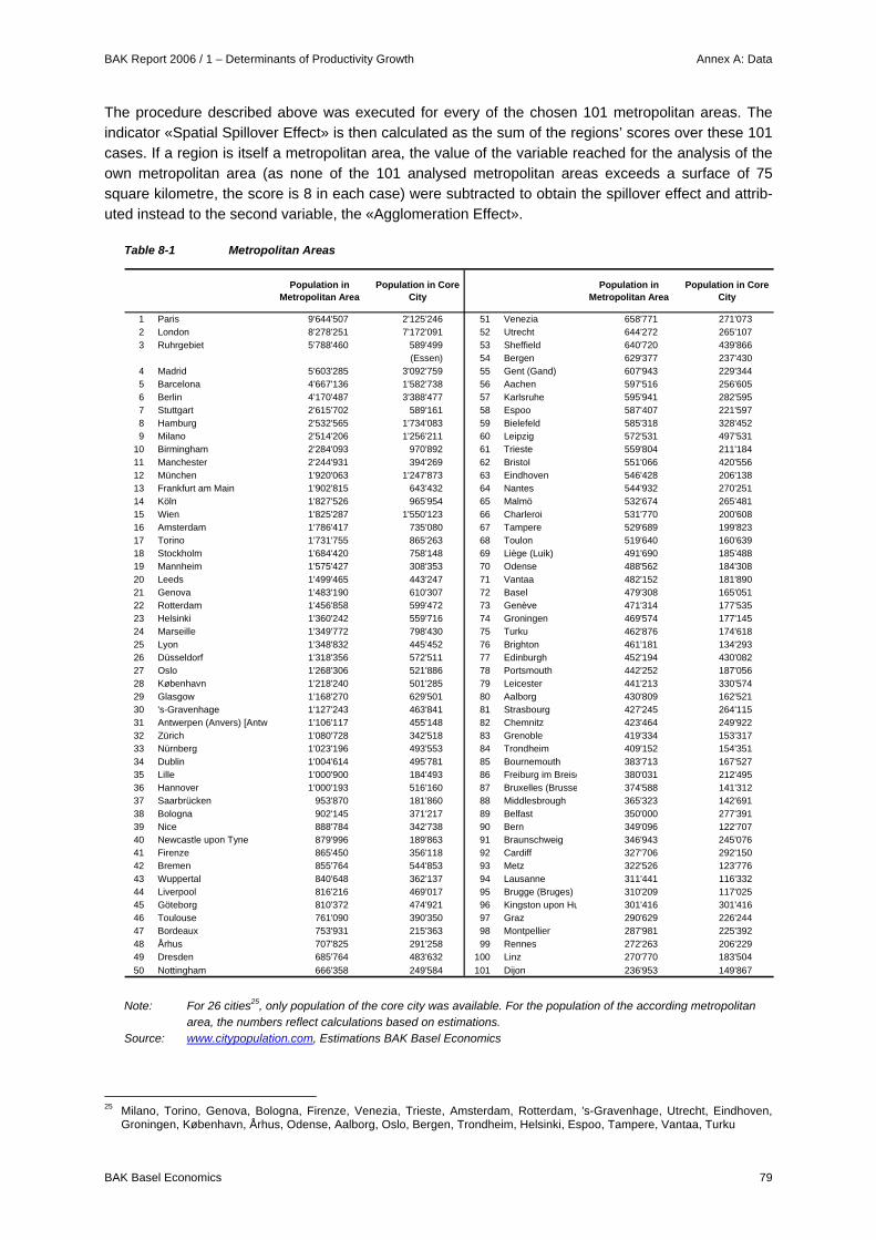
BAK Report 2006 / 1 – Determinants of Productivity Growth Annex A: Data
BAK Basel Economics 79
The procedure described above was executed for every of the chosen 101 metropolitan areas. The indicator «Spatial Spillover Effect» is then calculated as the sum of the regions’ scores over these 101 cases. If a region is itself a metropolitan area, the value of the variable reached for the analysis of the own metropolitan area (as none of the 101 analysed metropolitan areas exceeds a surface of 75 square kilometre, the score is 8 in each case) were subtracted to obtain the spillover effect and attrib-uted instead to the second variable, the «Agglomeration Effect».
Table 8-1 Metropolitan Areas
Population in Metropolitan Area
Population in Core City
Population in Metropolitan Area
Population in Core City
1 Paris 9'644'507 2'125'246 51 Venezia 658'771 271'0732 London 8'278'251 7'172'091 52 Utrecht 644'272 265'1073 Ruhrgebiet 5'788'460 589'499 53 Sheffield 640'720 439'866
(Essen) 54 Bergen 629'377 237'4304 Madrid 5'603'285 3'092'759 55 Gent (Gand) 607'943 229'3445 Barcelona 4'667'136 1'582'738 56 Aachen 597'516 256'6056 Berlin 4'170'487 3'388'477 57 Karlsruhe 595'941 282'5957 Stuttgart 2'615'702 589'161 58 Espoo 587'407 221'5978 Hamburg 2'532'565 1'734'083 59 Bielefeld 585'318 328'4529 Milano 2'514'206 1'256'211 60 Leipzig 572'531 497'531
10 Birmingham 2'284'093 970'892 61 Trieste 559'804 211'18411 Manchester 2'244'931 394'269 62 Bristol 551'066 420'55612 München 1'920'063 1'247'873 63 Eindhoven 546'428 206'13813 Frankfurt am Main 1'902'815 643'432 64 Nantes 544'932 270'25114 Köln 1'827'526 965'954 65 Malmö 532'674 265'48115 Wien 1'825'287 1'550'123 66 Charleroi 531'770 200'60816 Amsterdam 1'786'417 735'080 67 Tampere 529'689 199'82317 Torino 1'731'755 865'263 68 Toulon 519'640 160'63918 Stockholm 1'684'420 758'148 69 Liège (Luik) 491'690 185'48819 Mannheim 1'575'427 308'353 70 Odense 488'562 184'30820 Leeds 1'499'465 443'247 71 Vantaa 482'152 181'89021 Genova 1'483'190 610'307 72 Basel 479'308 165'05122 Rotterdam 1'456'858 599'472 73 Genève 471'314 177'53523 Helsinki 1'360'242 559'716 74 Groningen 469'574 177'14524 Marseille 1'349'772 798'430 75 Turku 462'876 174'61825 Lyon 1'348'832 445'452 76 Brighton 461'181 134'29326 Düsseldorf 1'318'356 572'511 77 Edinburgh 452'194 430'08227 Oslo 1'268'306 521'886 78 Portsmouth 442'252 187'05628 København 1'218'240 501'285 79 Leicester 441'213 330'57429 Glasgow 1'168'270 629'501 80 Aalborg 430'809 162'52130 's-Gravenhage 1'127'243 463'841 81 Strasbourg 427'245 264'11531 Antwerpen (Anvers) [Antw 1'106'117 455'148 82 Chemnitz 423'464 249'92232 Zürich 1'080'728 342'518 83 Grenoble 419'334 153'31733 Nürnberg 1'023'196 493'553 84 Trondheim 409'152 154'35134 Dublin 1'004'614 495'781 85 Bournemouth 383'713 167'52735 Lille 1'000'900 184'493 86 Freiburg im Breisg 380'031 212'49536 Hannover 1'000'193 516'160 87 Bruxelles (Brusse 374'588 141'31237 Saarbrücken 953'870 181'860 88 Middlesbrough 365'323 142'69138 Bologna 902'145 371'217 89 Belfast 350'000 277'39139 Nice 888'784 342'738 90 Bern 349'096 122'70740 Newcastle upon Tyne 879'996 189'863 91 Braunschweig 346'943 245'07641 Firenze 865'450 356'118 92 Cardiff 327'706 292'15042 Bremen 855'764 544'853 93 Metz 322'526 123'77643 Wuppertal 840'648 362'137 94 Lausanne 311'441 116'33244 Liverpool 816'216 469'017 95 Brugge (Bruges) 310'209 117'02545 Göteborg 810'372 474'921 96 Kingston upon Hu 301'416 301'41646 Toulouse 761'090 390'350 97 Graz 290'629 226'24447 Bordeaux 753'931 215'363 98 Montpellier 287'981 225'39248 Århus 707'825 291'258 99 Rennes 272'263 206'22949 Dresden 685'764 483'632 100 Linz 270'770 183'50450 Nottingham 666'358 249'584 101 Dijon 236'953 149'867
Note: For 26 cities25, only population of the core city was available. For the population of the according metropolitan area, the numbers reflect calculations based on estimations.
Source: www.citypopulation.com, Estimations BAK Basel Economics
25 Milano, Torino, Genova, Bologna, Firenze, Venezia, Trieste, Amsterdam, Rotterdam, 's-Gravenhage, Utrecht, Eindhoven,
Groningen, København, Århus, Odense, Aalborg, Oslo, Bergen, Trondheim, Helsinki, Espoo, Tampere, Vantaa, Turku

Annex A: Data BAK Report 2006 / 1 – Determinants of Productivity Growth
80 BAK Basel Economics
To illustrate the calculation of the two indicators, the example of the metropolitan area Greater London is described. Figure 8-1 shows the geographical units relevant for this example, Table 8-2 the classifi-cation of the regions into the six categories, and in table 10-3 the according indicator values for the regions involved.
Figure 8-1 Agglomeration and Spillover Effect: the example of Greater London
25075
BrightonPortsmouth
Bournemouth
Kingston upon HullSheffield
Liverpool
Leicester
Cambridge
Oxford
Leeds
Birmingham
Bristol
Cardiff
Manchester
Nottingham
Wales
South West
South East
East of England
East Midlands
Yorkshire and the Humber
West Midlands
London150
metropolitan areas
economic centre
Source: BAK Basel Economics

BAK Report 2006 / 1 – Determinants of Productivity Growth Annex A: Data
BAK Basel Economics 81
Table 8-2 Agglomeration and Spillover Effect: the example of Greater London I
region completely covered 1 Greater London
region only partly covered, centre of region covered 1 Greater London
region only partly covered, centre of region not covered 1 Greater London, East of England, South East
region completely covered 1 Greater London, East of England, South East
region only partly covered, centre of region covered 1 Greater London, East of England, South East, East Midlands, West Midlands, South West
region only partly covered, centre of region not covered 1 Greater London, East of England, South East, East Midlands, West Midlands, South West, Wales
75 K
M c
ircle
250
KM
circ
le
Source: BAK Basel Economics
Table 8-3 Agglomeration and Spillover Effect: the example of Greater London II
Points Population of Metro [Mio.] Indicator value
Agglomeration Effect
London 6 8.3 49.67
Spatial Spillover Effect
East of England 4 8.3 33.11
South East 4 8.3 33.11
East Midlands 2 8.3 16.56
West Midlands 2 8.3 16.56
South West 2 8.3 16.56
Wales 1 8.3 8.28
Source: BAK Basel Economics

Annex B: Econometric Methods BAK Report 2006 / 1 – Determinants of Productivity Growth
82 BAK Basel Economics
9 Annex B: Econometric Methods Annex B: Econometric Methods
9.1 Granger Causality The issue of causality is at the foundation of any study that examines an economic relationship. Gen-eral understanding of how a change in one variable affects another is paramount in comprehending economic behaviour and in formulating policy. Fortunately, economic theory is often available to help guide the building of models that are used to empirically examine the causal relationships among vari-ables. However, this is not always the case.
A methodology that has been used extensively in recent years to gain further insight into such situa-tions is Granger Causality (see Granger (1969)). To briefly explain how this methodology works, as-sume there are two time series, X and Y, where evidence is sought of a potential causal relationship. The following fundamental procedure is used to test for Granger Causality running from X to Y. If, while controlling for the information contained in past (lagged) values of Y, past (lagged) values of X add significantly to the explanation of current Y, then X is said to ‘‘Granger-cause’’ Y.
A symmetric test can also be performed to test for Granger Causality running from Y to X. If, while controlling for the information contained in lagged values of X, lagged values of Y add significantly to the explanation of current X, then ‘‘Y Granger-causes X.’’ A finding that only one of these relationships is true provides support for a unilateral line of causation. However, if both are found to be true, support for a bilateral (or jointly determined) relationship is provided. If neither relationship is found to exist, the assumption is made that the two variables are unrelated.
A more formal test for Granger Causality running from X to Y is shown as:
t
K
kktk
J
jjtjtt vXcYbaY +∗+∗+= ∑∑
=−
=−
11,
where vt is assumed to be a white noise error term and Yt-j and Xt-k represent the information con-tained in lagged values of Y and X. The number of lagged values (J and K) for the independent vari-ables is chosen by the investigator to adequately capture the integrity of the relationship.
To conduct the Granger Causality test, the above regression equation is estimated with and without the regressor matrix X followed by an F-test to test the null hypothesis that ck = 0 for k = 1,..,K. A rejec-tion of the null hypothesis implies that X Granger-causes Y. The formal test for Granger Causality running from Y to X is performed analogously. If the null hypothesis for each of the above Granger Causality tests is rejected, the evidence would indicate that the relationship between X and Y is bilat-eral, which implies they are jointly determined.
It should be noted that this methodology does not provide ‘‘proof ’’ of causation. The results from such tests should only be interpreted as showing that prior changes in one variable add (or do not add) significantly to the explanation of the future value of another variable. However, these Granger results do provide valuable information that existing ones.
9.2 Stationarity A common assumption in many time series techniques is that the data are stationary. A stationary process has the property that the mean, variance and autocorrelation structure do not change over time. If the time series is not stationary, we can often transform it to stationarity by building differences. The order of integration is the number of unit roots contained in the series, or the number of differenc-ing operations it takes to make the series stationary.

BAK Report 2006 / 1 – Determinants of Productivity Growth Annex B: Econometric Methods
BAK Basel Economics 83
Testing variables on stationarity before running regressions is necessary because standard inference procedures do not apply to regressions which contain an integrated dependent variable or integrated regressors. As a result, estimation results probably indicate a causal relationship between two vari-ables even if the result is just due to the fact that both variables underlie the same trend. Such results are known as «spurious regressions«.
The formal method to test the stationarity of a series is the Unit Root Test. The standard Dickey-Fuller test is carried out by estimating Equation
ttt uyy +⋅= −11α or ttt uyy +⋅=∆ −1δ respectively
The null hypothesis assumes that δ =0, tested with a conventional significance test.
Dickey and Fuller (1979) show that under the null hypothesis of a unit root, this statistic does not fol-low the conventional Student’s t-distribution, and they derive asymptotic results and simulate critical values for various test and sample sizes. MacKinnon (1991) implements a much larger set of simula-tions than those tabulated by Dickey and Fuller.
The simple Dickey-Fuller Unit Root Test described above is valid only if the series is an AR(1) proc-ess. If the series is correlated at higher order lags, the assumption of white noise disturbances is vio-lated. The Augmented Dickey-Fuller (ADF) test constructs a parametric correction for higher-order correlation by assuming that the series follows an AR(p) process and adding lagged difference terms of the dependent variable to the right-hand side of the regression:
tptpttt uyyyy +⋅++⋅+⋅= −−− ααα ..2211
After transformation the underlying equation of the test is
t
p
jjtjtt uyyy +∆⋅+⋅=∆ ∑
=+−−
211 βδ , with ∑∑
===−−=
p
ijii
p
ii αβαδ und )1(
1
or if a constant and time trend is included
t
p
jjtjtt uyyty +∆⋅+⋅++=∆ ∑
=+−−
21121 αδββ
The number of lagged difference terms is determined with the Akaike- or Schwartz-criterion, the Ljung-Box-Q-Statistics and significance-tests on the correspondent coefficients.
For panel data however, the classical time series AD-test, applied individually for each section (region) is not suited because of the lack of power. Indeed, the time dimension T=24 in our sample is too short to estimate the parameters in the ADF test. Recent literature suggests that panel-based Unit Root Tests have higher power than Unit Root Tests based on individual time series.
Panel Unit Root Tests are similar, but not identical, to Unit Root Tests carried out on a single series. Consider a following first-order Autoregressive process for panel data:
itititt uXyy +⋅+⋅= − δρ 11
where i=1,..,N cross-section units or series, that are observed over periods t=1,..,T.
The Xit represent the exogenous variables in the model, including any fixed effects or individual trends, δi are the autoregressive coefficients, and the errors uit are assumed to be mutually independent idio-syncratic disturbance. If | ρi|<1, yi is said to be weakly (trend-) stationary. On the other hand, if | ρi|=1, then yi contains a unit root. For purposes of testing, there are two natural assumptions that we can make about the ρi.
Annex B: Econometric Methods BAK Report 2006 / 1 – Determinants of Productivity Growth
84 BAK Basel Economics
First, one can assume that the persistence parameters are common across cross-sections so that ρi= ρ for all cross-sectional units. Alternatively, one can allow ρi to vary freely across cross-sections.
Two different Panel Unit Root tests have been applied in this study, namely the Levin/Lin/Chu-test (LLC) and the Im/Pesaran/Shin-test (IPS)26. The two principal drawbacks of the LLC are i) it does not allow for heterogeneity across sections (regions) as the autocorrelation coefficient is assumed to be the same for all regions, and ii) it does not take into account cross-sectional correlation. In contrast, IPS established by Im, Pesaran and Sin (1997) allows each region to have its own autocorrelation coefficient and is therefore preferable in our case. Nevertheless, both tests have been executed.
9.3 Autocorrelation and heteroscedasticity In a time series framework, autocorrelation and heteroscedasticity do not lead to inconsistent or bi-ased estimator, as long as the errors are orthogonal to the regressors. The only drawback is that mak-ing inference is no longer possible (statistical tests are no longer valid). However, in a panel frame-work, this may indicate the presence of unobserved heterogeneity through individual effects. In that case, the estimated parameters are inconsistent.
To test the pooled OLS residuals on autocorrelation, the Wooldridge test for autocorrelation in panel data was performed. Under the null of no serial correlation the residuals from the regression of the first-differenced variables should have an autocorrelation of -.5. This implies that the coefficient on the lagged residuals in a regression of the lagged residuals on the current residuals should be -.5. The Wooldridge test performs a Wald-test of this hypothesis.
To test for heteroscedasticity, the Likelihood ratio (LR) test was applied. The LR test is based on the comparison of two Cross-sectional time-series FGLS regressions, one with the underlying assumption of heteroscedasticity (and no autocorrelation) and one with the proposition of homoscedasticity. The LR test statistics is approximately chi-square distributed with degrees of freedom equal to the differ-ence of the dimensions of the unrestricted and restricted model). In our case, the first FGLS regres-sions involves the estimation of 109 covariances, while the restricted model only estimates one (ho-moscedasticity, so that the test statistics was chi2-distributedegree with 108 degrees of freedom.
9.4 Unobserved heterogeneity In a panel dataset, the pooled OLS estimator is the most efficient estimator among all others, it is said to be BLUE (Best Linear Unbiased Estimator). The problem is that it only holds under very restrictive assumptions (classical OLS assumptions). The key condition needed for pooled OLS to consistently estimate the parameters is that the disturbance term has mean zero and is uncorrelated with each of the repressors.
Pooled OLS does not allow any heterogeneity among sections (regions). Consequently, we ignore the heterogeneity among sections (regions), and so assume that all explanatory variables are exogenous. An explanatory variable is said to be endogenous if it is correlated with the error term. The endogene-ity leads to inconsistent and biased estimations in an OLS framework. Many causes can be responsi-ble for the endogeneity. The most current is the omitted variables. Indeed, in a panel dataset, it is very usual to have heterogeneity across section (in our case regions) without having a variable explaining it. Fixed effect and random effect allows taking into account to a certain extent unobserved effects and so avoiding the correlation between repressors and the error term.
Following the literature, we compare the OLS with RE (or FE) to determine whether heterogeneity across sections (regions) is present. The Breush-Pagan test is perfectly suited to test the presence of an unobserved effect. The Breusch-Pagan (1979) Lagrange multiplier test tests for heteroscedasticity
26 See Levin, Lin and Chu (2002) and Im, Pesaran and Shin (2003)

BAK Report 2006 / 1 – Determinants of Productivity Growth Annex B: Econometric Methods
BAK Basel Economics 85
in the error distribution, conditional on a set of variables which are presumed to influence the error variance. The test statistic, a Lagrange multiplier measure, is distributed Chi-squared(p) under the null hypothesis of homoscedasticity. The test is asymptotically equivalent to White's (1980) general test for heteroscedasticity if the same auxiliary variables are specified (for White's test, all distinct regressors, cross-products and squares of regressors). See Greene (2000), pp. 507-511.
9.5 Panel data methods The basic methods used in a in a panel data setting are the Fixed Effects Model and the Random Effects Model. They mainly differ in the way they take individual heterogeneity into account. The star-ting point is the simple model
ititt 'Xy ε+β⋅=
In extension to the standard regression model, the structure for the error term is of the form
itiit η+α=ε ,
where ηit follows the standard assumptions of the classical linear regression model. One of these as-sumptions is that ηit is uncorrelated with Xit.
It is the assumption about the first part of the error structure, namely the time-invariant term αi, whether one speaks of a fixed effects or a random effects model. Within the random effects frame-work, one assumes that αi is uncorrelated with Xit, while this restriction is not necessary within the fixed effects framework.
9.5.1 Fixed Effects Model As been said, within the fixed effects framework, αI is not assumed to be uncorrelated with Xit. The fixed effects model is simply a linear regression model in which the intercepts vary for the individual units i. Therefore the fixed effects approach implies that the individual heterogeneity is represented through a shift in the intercepts:
ititit 'Xy ε+β⋅+α=
Mention that αI is just treated as an unknown parameter, which has to be estimated. Because the number of individuals in typical panel settings is large and the number of periods is small, often prob-lems with the degrees of freedom arise.
To come along with this difficulty, one usually transforms the equation above in a way that the individ-ual effects are cancelled out (a common fixed effects estimator is the so called within estimator). The parameters of the individual effects are then determined indirectly through retransformation, although one can not obtain consistent estimates for these parameters in the typical panel case.

Annex B: Econometric Methods BAK Report 2006 / 1 – Determinants of Productivity Growth
86 BAK Basel Economics
9.5.2 Random Effects Model Within the random effects model the individual heterogeneity is introduced through an additional error component. The error term itiit η+α=ε consists of two components: an individual specific component
αI, which does not vary over time and a remainder component which is assumed to be uncorrelated over time.
As said, αI is assumed to be uncorrelated with Xit so that, along with the assumptions for ηit, the coeffi-cients of Xit, can be estimated unbiased with ordinary least squares (OLS). Two problems arise with using OLS however: First, OLS will produce consistent estimates of β but the standard errors will be understated. Second, OLS is not efficient compared to a feasible generalised least-squares (GLS) procedure by exploiting the structure of the error covariance matrix.27 The GLS procedure is a regres-sion technique that is usually attended when the error terms from an ordinary least squares regression display non-random patterns such as autocorrelation or heteroscedasticity.
The GLS estimator is sometimes referred to as a weighted least squares estimator, because it is a least squares estimator in which each observation is weighted by a factor proportional to the inverse of the error variance. The use of weights implies that observations with a higher variance get a smaller weight in the estimation. In other words, the greatest weights are given to observations of the highest quality and the smallest weights to those of the lowest quality.28
9.5.3 Hausman-test A widely used class of tests in econometrics is the Hausman test (Hausman (1978)). The underlying idea of the Hausman test is to compare two sets of estimates, one of which is consistent under both the null and the alternative (the fixed effects model) and another which is consistent only under the null hypothesis (the random effects model). A large difference between the two sets of estimates is taken as evidence in favour of the alternative hypothesis.
In other words: The Hausman test tests the null hypothesis that the coefficients estimated by the effi-cient random effects estimator are not systematically different from the ones estimated by the consis-tent fixed effects estimator. In fact, the Hausman test is based on estimating the variance var(βRandom
Effects-βFixed Effects)of the difference of the estimators by the difference var(βRandom Effects)-var(βFixed Effects) of the variances. The test statistic is chi2 distributed with a degree of freedom according to the dimension of the variance matrix (number of regressors).
If the Hausman test suggests that the coefficients are not systematically different, it’s safe to use ran-dom effects. A Fixed effects model is also consistent in that case, but the random effects model leads to a more efficient estimator. Otherwise, if the Hausman test suggests systematic differences between the two estimators, a fixed effects model has to be applied.
27 See Johnston and DiNardo (1997), p.391, Verbeek (2000), p. 315. 28 See Verbeek (2000), p.78.
BAK Report 2006 / 1 – Determinants of Productivity Growth Annex C: Summaries of Selected Studies
BAK Basel Economics 87
10 Annex C: Summaries of Selected Studies Annex C: Summaries of Selected Studies In the following selected empirical studies of determinants of growth are summarised.
Ahmed, H. and S. Miller, (1999), «The level of development and the determinants of productivity growth» Pooled OLS, RE and FE estimations for three different country samples (low-income countries, middle-income countries, high-income countries) in a sample of 93 countries from 1976 to 1984. The productivity growth rate is regressed on investment to GDP, population growth and parameters of the production function to find out the specificity in each group of country. The main result is that investment is the most important determinant of productivity growth for low-income countries (mostly African countries), while for middle-income countries, additional ef-fects like technological change are important. However, for high-income countries, investment is not significant any more, but solely technological change. The results of this paper can be used to justify why in the project BAK regional growth rate investment has not been investi-gated. The population growth rate affects productivity growth negatively both in low- and high-income countries, but does not significantly affect productivity growth in middle-income coun-tries. The analysis also gives an explanation for the slow down of productivity growth in high-income countries. Expansion of the low-productivity service sector and the decrease in the share of the high-productivity industrial (manufacturing) sector pulls down real productivity growth. Thus, in high-income countries, productivity growth can increase if the industrial sector share expands, or the level of technology in the expanding service sector is raised.
Barro, R. (1998), «Determinants of economic growth: a cross-country empirical study» The regression framework is applied to a panel of data covering roughly a hundred countries over the years 1968-1990 in an effort to determine what factors are important in explaining long-run growth. The findings highlights that the growth rate of real per capita GDP is en-hanced by better maintenance of the rule of law, smaller government consumption, longer life expectancy, more male secondary and higher levels of schooling, lower fertility rates, and im-provements in the terms of trade. The data also support the notion of conditional convergence; that is, for given values of these variables, countries with a lower initial level of real per capita GDP grow faster. The analysis also looks at democracy and inflation as potential factors de-termining growth rates. In chapter II, he looks at the role of political freedom in determining growth rates. The positive relation between democracy and prior measures of prosperity is well established as an empirical regularity. The third chapter considers the effects of inflation on long-run economic performance. The clear evidence for adverse effects of inflation from the experiences of high inflation (annual rates in excess of 20%).
Bassanini, A. and S. Scarpetta, (2001), «The driving forces of economic growth: panel data evidence for the OECD countries»Panel VECM to estimate cross-country (OECD countries) differences in GDP growth perform-ance as well as the evolution of performance over time in each country. Bassanini and Scar-petta choose a pool mean group estimator that allows intercepts, the convergence parameter, short run coefficients and error variances to differ across countries, but imposes homogeneity on long-run coefficients. Accumulation of physical capital as well as human capital (main driv-ers of economic growth) turned out to be essential. In addition, R&D activity (expenditures on

Annex C: Summaries of Selected Studies BAK Report 2006 / 1 – Determinants of Productivity Growth
88 BAK Basel Economics
R&D), sound macroeconomic environment (low inflation, small government deficit, large gov-ernment sector), trade openness and well-developed financial markets contribute to raise GDP in OECD countries.
Brakman, S., H. Garrestsen and M. Schramm, (2002), «New economic geography in Germany: testing the Helpman-Hanson model» According to the paper, the spatial characteristics of the German economy can be explained by the New Economic Geography by means of a WLS (Weighting Least Square) they find that all parameters of the wage equation are significant and have the right sign.
Brakman, S., H. Garretsen and M. Schramm, (2004), «Putting new economic geography to the test: free-ness of trade and agglomeration in the EU regions» Based on an estimation of the equilibrium wage equation from the NEG, Brakman et al. find evidence that economic integration leads only to agglomeration for regions that are relatively close to each other. In Europe, agglomeration seems to be most relevant at lower geographical scales because of the lack of labour mobility.
Ciccone, A. and R. Hall, (1996), «Productivity and the density of economic activity» Two hypothesis of the NEG were tested: the local geographical externalities and the diversity of local intermediates services. Both theoretically lead to Increasing Return to Scale. Ciccone and Hall show that, first the density of economic activity at the county level is crucial for ex-plaining the variation of productivity at the state level. The doubling of employment density explains a 6% increase of average labour productivity. The econometrical methodology is a cross-sectional OLS regression.
Davis, D. and D. Weinstein, (1998), «Market access, economic geography and comparative advantage: an empirical as-sessment» Existence of «home market effects» (theoretical concept by Krugman) if the importance of market access in implementing models of economic geography is taken into account.
De la Fuente, A, (2002b), «The effect of structural fund spending on the spanish regions: an assessment of the 1994-99 objective1 CSF» The EU structural policy impinged positively on the regional GDP of about 1% and 0.4% of employment creation per year. Besides, the convergence reduced the gap between regions at 20% over the period considered. The results are based on a supply side model. The coeffi-cients of physical capital accumulation, infrastructure and human capital are all three positive and statistically significant in a fixed effect model.
De la Fuente, A, (2003), «Does cohesion policy work? Some general considerations and evidence from Spain»Empirical investigation with the following results: EU regional structural policy has a positive impact on regional GDP particularly when funding investment in human capital (education) and

BAK Report 2006 / 1 – Determinants of Productivity Growth Annex C: Summaries of Selected Studies
BAK Basel Economics 89
to a fewer extent in infrastructure. Investing in infrastructure has a positive impact for low GDP regions with weak infrastructure, but once reached a high infrastructure standard (saturation effect), investment is no longer effective.
De la Fuente, A, R. Doménech and J. Jimeno, (2003) «Human capital as a factor of growth and employment at the regional level. The case of Spain» First, the effects of school attainment on individual wages, participation rates and employment probabilities in Spain are quantified; second, the contribution of education to labour productivity at the regional level is measured. These results are used to estimate the private and social returns to schooling. First, using Weighted Least Squares and allowing wage correlation within firms, they find that schooling has a strong positive impact on wages. Second, with a probit two-stage procedure they show that schooling has a positive impact on labour force participa-tion and employment probabilities.
De la Fuente, A. (2002), «Convergence across countries and regions: theory and empirics» Discussion about the relevance of beta and sigma convergence (among regions within a coun-try). The author argues that panel econometrics is not always relevant for convergence analy-sis.
Dewan, E. and S. Hussein, (2001), «Determinants of economic growth» Panel econometrics methodology with fixed effects and random effects estimators are used to explain the GDP growth rate in developing countries (41 middle-income countries). The de-pendent variables are first differenced and are: labour force, gross domestic investment, infla-tion, import goods, public spending on education, good imports. The results show that coun-tries with strong macroeconomic fundamentals (change in inflation ->low inflation, ) tend to grow faster, but also change in investment in both physical and human capital (public spending on education), open trade policies (less trade barriers), are necessary for economic growth. The change in technology (capacity to adopt technological changes) is essential too.
Feenstra, R. J. Markusen and A. Rose, (1998), «Understanding the home market effect and the gravity equation: the role of differenti-ating goods» Quantification of the home market effect using cross-sectional gravity equations. Domestic income export elasticities are indeed substantially higher for differentiated goods than for ho-mogeneous goods
Gustavson, P. and J. Persson, (2003), «Geography, cost-of-living, and determinants to economic growth: a study of the swedish regions, 1911-1993» This paper analyses determinants to economic growth with a spatial perspective using data on the Swedish counties for the period 1911-1993. First the authors analyse spatial interdepen-dency in regional income per capita growth rates, and find robust and significant evidence for spatially autocorrelated growth rates, that is, growth rate in one county are found to be de-pendent on growth rates in contiguous counties. Additional channels of geographical growth
Annex C: Summaries of Selected Studies BAK Report 2006 / 1 – Determinants of Productivity Growth
90 BAK Basel Economics
spillover were found, i.e., the income per capita, and market size spillover. Agglomeration, measured by population density, has a positive effect on the growth rate of income per capita. Among the control variables, only the net migration is found to have a negative robust impact on per capita income growth independently whether income is PPP adjusted or not. The eco-nometric tools are 2 Stage Least Square estimators.
Hall, R. and C. Jones, (1998), «Why do some countries produce so much more output per worker than others?» In a cross-sectional OLS estimates, including 127 countries, they prove that high level of output per worker is achieved in the long run because of high investment rates in physical capital, human capital and high level of productivity (production function). These variables are driven positively in countries where social infrastructure is well developed. This social infrastructure means institutions and government policies that make up the economic environment within which individuals and firms make investments, create and transfer ideas, and produce goods and services.
Kaldewei, C. and U. Walz, (2001), «The determinants of regional growth in Europe: an empirical investigation of regional growth models» With a sample from 1980 to 1996 and using regional data at the NUTS-2-level, Kaldewei and Walz investigate an empirical study of determinants of GDP per capita growth. The economet-ric methodology is of the easiest one: pooled OLS. They combine elements of the New Econ-omy Geography and Endogenous Growth theory and find evidence that the average growth rate of GDP per capita depends positively on, the accumulation of human capital, the agglom-eration effect, transport costs (or access to market), financial sector and negatively on migra-tion, population density and population size. However, regional knowledge spillovers, regional transfers and transport costs are not significant. Regional knowledge spillovers are approxi-mated with the number of patents. Transfers and transport costs on the other hand have oppo-site effects on GDP growth. At first sight transfers have a positive effect, but they also hinder structural adjustment. Transport costs have theoretically non linear effects on GDP and so this result (the fact that transport costs are not significant) is also justified. To control for industrial structure, they include the share of employment in agriculture and share of employment in the service sector. Finally they investigate the beta convergence hypothesis (absolute and condi-tional), and find evidence for it but lower than 2% (2% are the estimate of Barro and Sala-i-Martin).
K L Krishna, (2004), «Patterns and determinants of economic growth in Indian States» The paper studies economic performance of Indian States during the period 1960-2000. Using panel fixed effect estimator, he finds evidence. In developing countries, the size of the agricul-tural sector has a positive impact on industrial and service sector growth. Besides, social infra-structure is an important determinant of the investment decisions.
Moreno, R., M. Artis, E. López-Bazo and J. Suriñach, (2000), «Evidence on the complex link between infrastructure and regional growth» Analysis of the link between public infrastructure and productivity in Spanish regions. Infra-structure has a positive but modest effect on productivity. The existence of spatial autocorrela-

BAK Report 2006 / 1 – Determinants of Productivity Growth Annex C: Summaries of Selected Studies
BAK Basel Economics 91
tion with other regions (spatial spillover) makes the link between productivity and regional pro-ductivity very complex. Taking into account this autocorrelation effect, there is little evidence of a positive-link infrastructure-growth. But public infrastructure is a prerequisite to economic ac-tivity and so essential.
Overman, H., S. Redding and A. Venables, (2001), «The economic geography of trade, production, and income: a survey of empirics» Geography is a major determinant of factor prices, and the degree of access to foreign market (transport costs, time costs, fixed costs, barrier to enter new foreign markets) is shown to ex-plain some 35% of the cross-country variation in per capital income. The paper documents empirical findings of home market effects, suggesting that imperfectly competitive industries are drawn more than proportionally to locations with good market access.
Vayà, E., E. López-Bazo and M. Artis, (2000) «Growth convergence and (why-not?) regional externalities» Investigation of the question how important regional spillover in regional convergence is. The distinguish demand driven externalities (approximated by the weighted growth rate in the re-gion’s neighbours) while the supply-side would be by the initial level of the neighbours. Both effects are robust to different specifications. Demand-side externality seems to be stronger than supply-side externalities.