Determinants of National Debt: Evidence from the Greek

DETERMINANTS OF NATIONAL DEBT: EVIDENCE FROM THE GREEK ECONOMY IN THE LAST DECADE

Dr. Kalimeris Dimitrios, Adjunct Lecturer at the University of Macedonia, Department of Marketing and Operations Management, 156 Egnatia street, Postal Code 540 06,

Thessaloniki, Greece e-mail: [email protected]

Abstract In an attempt to emphasize on Greece’s economic problem and lending credibility as a victim of the neoliberal economic approach, this research paper attempts to examine some important macroeconomic factors, like the intra and extra-EU trade balance and long term interest rates on government bonds in relation with national debt levels of Greece in the past decade. Granger causality and VAR results agree that current national debt is granger-caused by the majority of these factors, while on the other hand, it is responsible for the country’s poor intra-EU trade balance. Keywords: National debt, Granger causality, VAR methodology JEL classification: E20-General Macroeconomics, E61-Policy Objectives; Policy Designs and Consistency; Policy Coordination, F34-International Lending and Debt Problems, F41-Open Economy Macroeconomics 1. Introduction

Current economic facts like the economic crisis we are dealing with since 2007 are being analyzed in terms of macroeconomic variables, such as GDP per capita, government deficit, national debt, and so on. The case of Greece is a characteristic example in where every part of its socio-economic life, the working classes, the press, the government, foreign and domestic investors, are trying to distinguish the causes of such a great national debt. The effects are rather easier to distinguish than the causes. The country’s foreign debt has grown from 125% in 2009 to 144% of GDP in 2010, while fiscal deficit declined form 15,4% in 2009 to a low 9,5% in 2010. Of course, there must be a case of interrelationship between the two deficits, while many believe that the first (national debt) finances the second, in order to improve the country’s market position. From 1998, and even earlier, Greece’s national debt has a steady rising trend, with a short break in 2004-2005, due to the Olympics hosting.

The imposition of the International Monetary Fund (IMF) funding rules on Greece in combination with an eighty billion euros loan from the eurozone can be considered as the result of a chronic mismanagement of domestic fiscal policy by both political parties in power in the last thirty five years. The current government tries to meet the IMF’s lending conditions by using extreme public finance measures, such as lowering taxation on capital and raising it on consumption. Recent information disseminated from the press shows that the Greek prime minister asked for the IMF’s help only two weeks after achieving his position, and after promising that the country has enough money to deal with the crisis. Of course, he could have meant IMF’s money. On the contrary, the financial aid has taken the form of decrease in public expenditure and rising of taxes. This has been a popular technique in dealing with economic crises throughout history. In the case of Greece, inflation pressures were inevitable, but new and harder taxes on low wage earners silenced the inflation humming just by making consumption ever more costfull. Levels of investment have deteriorated even further, since lower consumption means even lower savings from private agents. As a final blow, the government imposed severe cuts on public expenditure as an excuse to finance the country’s debt, while the only ones that are actually being financed are Greece’s lenders, and by that we mean the investors who bought government bonds and the IMF. It is interesting to mention some countries that are being financed by the IMF, along with Greece; other countries are Angola, Antigua and Barbuda, El Salvador, Georgia, Honduras, Iraq, Jamaica, the Republic of Latvia, Maldives, Pakistan, ant others.

The fact that Greece’s government deficit fell is only due to the heavy taxation of middle and low classes and to the cut of public expenditure, mainly in the form of pay cuts and dismissals in the public sector. All these facts can lead to severe economic questions, like: What are the determinants of a country’s national debt? Can the lowering of government deficit be of any assistance in dealing with it? Are the long term interest rates of Greece’s government bonds a result of the country’s twin deficit situation? Do internal (inside the European Union), or external trade balances affect Greece’s national debt?

Dr.Kalimeris Dimitriosi, et.al., Int. J. Eco. Res., 2011 2(5), 22-32 ISSN: 2229-6158

IJER | SEPTEMBER - OCTOBER 2011 Available [email protected]

22

The rest of the paper is structured as follows: The second part refers to the literature review that deals with explaining and evaluating the causes and effects of national and government debt in several cases. Part three analyses the data used for this research, the econometrics used and the methodology adopted; Part four holds the analysis’ results and discuses the issued awaken; The fifth part is an Appendix of the tables referred to in the main body of the paper; Finally, the sixth part list the references used. 2. Literature Review

Boskin M. J. (2004) tried to explain the ‘dangers’ in decoding government deficit and

national debt. He, specifically, distinguished between the usual measures of them and the variables that affect them. ‘The usual measures of the deficit and debt can be extremely misleading. The deficit is heavily affected by the business cycle. Inflation erodes the value of the previously issued national debt, i.e., the real debt declines with inflation (and conversely increases with deflation)’.

Raghbendra Jha (2001) tried to evaluate the effects of fiscal policy on macroeconomic adjustment in developing countries. Conventional measuring of deficits hides many difficulties, such as the inability to evaluate the different that tax and expenditure have on aggregate demand, and the fact that tax revenues are endogenous of expenditures. She also comments on the fact that, since the late 1980s, developing countries have experienced surges in capital inflows, according to the World Economic Outlook. These inflows, apart form being welcomed, caused serious challenges for the conduct of monetary policy.

Daniel C.B. and Shiamptanis C. (2008) investigated the way a fiscal policy could behave in a state of financial crisis. The behavior or response of the fiscal policy could affect the timing and the probability of the crisis. They authors tried to simulate fiscal risk under two alternative fiscal responses to a crisis, and concluded that, for countries like Greece and Italy, with high debt, are not to be considered safe. Since fiscal policy is not coordinated among member states of the EU, it is quite difficult to expect an overall and synchronized encounter of the financial crisis.

Schreft S. L. and Smith B. D. (2003) investigated the effect of reducing government debt stock on welfare. Using a model economy with three assets, they concluded that if there is money creation, risk-taking agents, and there is a primary government budget deficit, a positive stock of government debt is optimal. Apart from that, the help of government bonds in raising welfare is discussed. Most of the literature on the subject indicates that markets are incomplete in the form of borrowing constraints. The role of risk-free government bonds creates several opinions. Some believe that they are socially beneficial, since they have a risk-free rate of return, while others argue that the same kind of benchmark can be provided by the private sector.

Bertrand C., Muysken J., and Vermeulen R. (2007) in an attempt to analyze the stability of fiscal rules for EMU countries before and after the Maastricht Treaty, they distinguished between discretionary and non-discretionary fiscal policy. In conclusion, the evaluation of the impact of the Maastricht Treaty implies that automatic stabilizers are more effective in counter-cyclical stabilization after the Treaty’s implementation, while the procyclical stance of applying discretionary fiscal policy before the signing of the Treaty turns to acyclical stance. For countries that have moved to the ‘safe area’ of 3% deficit ratio, the pressure to continue towards the goal of balance or surplus is much weaker.

Tobin J. (2001) questioned the ‘permanent’ reduction in federal income and estate taxes that President George W. Bush imposed in 2001. At that time, the need for measures was more of quick and temporary measures that could correspond to the almost full-employment level of the US economy at the time. Apart from that, a monetary policy for stabilizing the job market is proposed in the research. Several applied policies, those of former Fed Chairman’s Paul Volcker in 1982, President’s Reagan in the 1980s, and former Fed Chairman’s Greenspan are discussed and compared.



23

http://econpapers.repec.org/RAS/pca231.htm�

http://econpapers.repec.org/RAS/pmu106.htm�

http://econpapers.repec.org/RAS/pve149.htm�

3. Data and Methodology

3.1 Data

All of the data are extracted from the Eurostat database. The variable in research is the general government gross debt of Greece in the last 10-12 years, in millions of euro, expressed in percentage of GDP. We use the variable in the sense as the Maastricht Treaty describes it; as the general government gross debt at nominal value, outstanding at the end of the year. The general government sector comprises central government, state government, local government, and social security funds. Instead of the term ‘public debt’, we will use the term ‘national debt’ (variable ND). The data range is from 1998 to 2009 in yearly figures.

Several macroeconomic variables are found to affect the level of national debt in an economy. What we are trying to do in the current research, is to isolate the effects of particular variables, namely, government deficit, intra-EU trade balance, extra-EU trade balance, and long-term interest rates.

We use the variable ‘general government deficit’ in millions of euro as a percentage of GDP. It comprises of the central government’s and of the social security funds (variable GD). The data range is from 1998 to 2009 in yearly figures.

We define long-term interest rates as the annual average of the 10-year government bond yields traded in the secondary market. We prefer to use the specific kind of bonds because they are often used as a measure for long-term interest rates (variable IR). Secondary market means that the bond price is not an issue price (primary market) but determined by supply and demand on the market. The data range is from 1998 to 2007 in yearly figures.

For the effect of trade on national debt we use two variables, the first one being the country’s contribution (in value and percentage) to the intra-EU27 trade of the Union, and the second the country’s contribution (in value and percentage again) to the extra-EU27 trade of the Union (variables IETB and EETB respectively). The data range for both variables is form 1999 to 2009 in yearly figures.

Before moving on to the methodology adopted we should address the issue of stationarity check. By conducting individual unit root tests for our variables we reached the following results (Tables 3.1.a-3.1.e):

Stationarity tests: Tables 3.1.a-3.1.e: Table 3.1.a: Null Hypothesis: D(ND) has a unit root Exogenous: None Lag Length: 1 (Automatic based on SIC, MAXLAG=3) t-Statistic Prob.* Augmented Dickey-Fuller test statistic -1.644557 0.0925 Test critical values: 1% level -2.847250 5% level -1.988198 10% level -1.600140 *MacKinnon (1996) one-sided p-values. Warning: Probabilities and critical values calculated for 20 The ND variable is stationary at 1st difference at a 10% confidence interval.



24

Table 3.1.b: Null Hypothesis: D(IETB,2) has a unit root Exogenous: Constant, Linear Trend Lag Length: 1 (Automatic based on SIC, MAXLAG=1) t-Statistic Prob.* Augmented Dickey-Fuller test statistic -4.741369 0.0388 Test critical values: 1% level -6.292057 5% level -4.450425 10% level -3.701534 *MacKinnon (1996) one-sided p-values. The IETB variable is stationary at 2nd difference at a 5% confidence interval. Table 3.1.c: Null Hypothesis: D(EETB,2) has a unit root Exogenous: None Lag Length: 0 (Automatic based on SIC, MAXLAG=1) t-Statistic Prob.* Augmented Dickey-Fuller test statistic -2.498261 0.0201 Test critical values: 1% level -2.886101 5% level -1.995865 10% level -1.599088 *MacKinnon (1996) one-sided p-values. The EETB variable is stationary at a 2nd difference at a 5% confidence interval Table 3.1.d: Null Hypothesis: D(GD,2) has a unit root Exogenous: None Lag Length: 0 (Automatic based on SIC, MAXLAG=1) t-Statistic Prob.* Augmented Dickey-Fuller test statistic -1.979251 0.0524 Test critical values: 1% level -2.937216 5% level -2.006292 10% level -1.598068 *MacKinnon (1996) one-sided p-values. The GD variable is stationary at a 2nd difference at the 10% confidence interval Table 3.1.e: Null Hypothesis: IR has a unit root Exogenous: None Lag Length: 0 (Automatic based on SIC, MAXLAG=1) t-Statistic Prob.* Augmented Dickey-Fuller test statistic -2.774739 0.0114 Test critical values: 1% level -2.847250 5% level -1.988198 10% level -1.600140 *MacKinnon (1996) one-sided p-values.



25

The IR variable is stationary at level. Therefore, by retrieving stationary series, we move on to methodology adopted.

3.2 Methodology By applying the hypothesis that there are no exogenous variables that affect national debt

in our set of variables, we use the methodology of VAR analysis. Furthermore, we are willing to investigate whether there is any kind of granger-causality among our variables. More specifically, one of the implications of this theorem is that of any two variables, Xt and Yt, are cointegrated and each one is individually integrated of order 1 (each is individually non-stationary), then either Xt must granger-cause Yt or the opposite. Not only do we care about any signs of granger-causality, but also about its direction of causality. In our model, we have five variables; therefore we could end up with a set of five different regressions. Instead of that we regressed national debt with each one separately to avoid and effects from the loss of degrees of freedom in our results’ analysis. Furthermore, we applied a set of VAR analysis between the variables government debt and long term interest rates.

Along with our VAR analysis, we conducted pairwise granger causality test among the variables, in order verify our findings.

In the case of a two-variable model with Xt and Yt, vector auto-regression is a set of two equations, each of which contains κ lag values of of Xt and Yt:

Xt = +a ∑ ∑= =

−− ++k

j

k

jtjtjjtj uYX

1 1γβ (2)

And Yt = a ′+∑ ∑= =

−− ++k

j

k

jtjtjjtj uXY

1 1γβ (3)

where, Xt and Yt are column vectors of observations at time t on the two variables, the ut’s are the stochastic error terms (or innovations or shocks).

In our case, the four sets of vector auto regressions we examined are: Examining the VAR relationship between: National Debt and Government deficit Using two lags for both variables provided us with not statistically significant results; therefore, we used only one lag for each variable:

tttt uGDNDND +++= −− 11 γβα

tttt uNDGDGD +++= −− 11 γβα National debt and Intra-EU trade balance

tttttt uIETBIETBNDNDND +++++= −−−− 22112211 γγββα

tttttt uNDNDIETBIETBIETB +++++= −−−− 22112211 γγββα National debt and Extra-EU trade balance

tttttt uEETBEETBNDNDND +++++= −−−− 22112211 γγββα

tttttt uNDNDEETBEETBEETB +++++= −−−− 22112211 γγββα National debt and long term interest rates

tttttt uIRIRNDNDND +++++= −−−− 22112211 γγββα

tttttt uNDNDIRIRIR +++++= −−−− 22112211 γγββα In order to strengthen our final results, we use pairwise granger causality test for all the

variables. After retrieving both the VAR and the granger tests, we compare them and try to find any similarities. Since we have five variables in total, our granger test pairs are ten, and in particular:



26

Table 3.2.a: Pairwise Granger Causality Tests ND↔GD GD↔EETB ND↔ IETB GD↔ IR ND↔EETB IETB↔EETB ND↔ IR IETB↔ IR GD↔ IETB EETB↔ IR

The ↔ symbol represents granger causality that runs both ways. We examined all three different aspects of causality direction (two unilaterals and one bilateral), as it can be seen in the results below.

4.Results and Discussion

First of all, we can examine our results in the pairwise granger causality tests, which are:

Table 4.a: Pairwise Granger Causality Tests Sample: 1998 2009 Lags: 2 Null Hypothesis: Obs F-Statistic Probability GD does not Granger Cause ND 8 1.40619 0.37081 ND does not Granger Cause GD 0.31377 0.75208 IETB does not Granger Cause ND 9 1.64528 0.30102 ND does not Granger Cause IETB 7.78146 0.04181 EETB does not Granger Cause ND 9 3.49496 0.13247 ND does not Granger Cause EETB 1.45045 0.33598 IR does not Granger Cause ND 8 5.75362 0.09404 ND does not Granger Cause IR 0.02398 0.97649 IETB does not Granger Cause GD 8 0.80979 0.52333 GD does not Granger Cause IETB 0.59530 0.60571 EETB does not Granger Cause GD 8 13.8460 0.03056 GD does not Granger Cause EETB 5.21983 0.10546 IR does not Granger Cause GD 6 0.50629 0.70489 GD does not Granger Cause IR 2.30810 0.42197 EETB does not Granger Cause IETB 9 1.16122 0.40027 IETB does not Granger Cause EETB 0.05903 0.94349 IR does not Granger Cause IETB 7 2.89439 0.25678 IETB does not Granger Cause IR 0.48221 0.67467 IR does not Granger Cause EETB 7 0.34866 0.74147 EETB does not Granger Cause IR 0.28009 0.78120 (Note: The test’s critical values (of the F test) are: 2,28 at 25%, 5,46 at 10% and 9,55 at 5%. The pairs in bold denote the existence of one-way granger causality).

Therefore, our tests show that there are three cases of unilateral granger causality, directing form national debt to intra-EU trade balance, from long run interest rates to national debt, and from extra-EU trade balance to government deficit.

Our VAR equations in pairs provided us with the following results: +



27

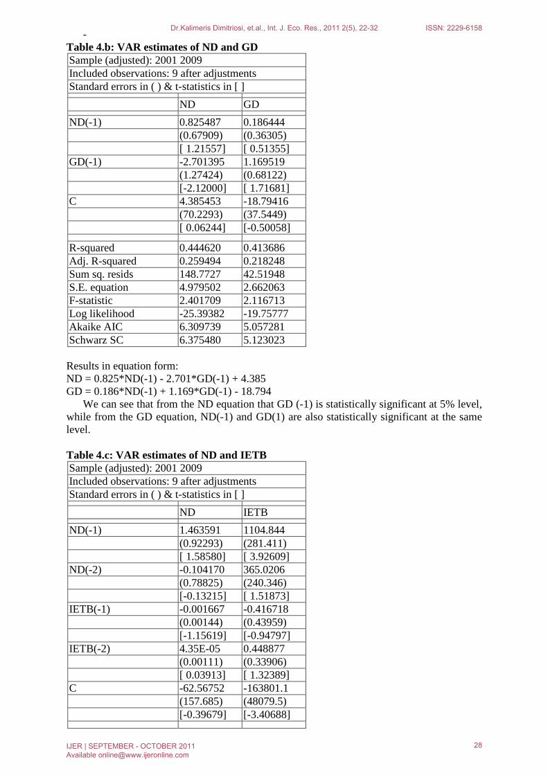
- Table 4.b: VAR estimates of ND and GD Sample (adjusted): 2001 2009 Included observations: 9 after adjustments Standard errors in ( ) & t-statistics in [ ] ND GD ND(-1) 0.825487 0.186444 (0.67909) (0.36305) [ 1.21557] [ 0.51355] GD(-1) -2.701395 1.169519 (1.27424) (0.68122) [-2.12000] [ 1.71681] C 4.385453 -18.79416 (70.2293) (37.5449) [ 0.06244] [-0.50058] R-squared 0.444620 0.413686 Adj. R-squared 0.259494 0.218248 Sum sq. resids 148.7727 42.51948 S.E. equation 4.979502 2.662063 F-statistic 2.401709 2.116713 Log likelihood -25.39382 -19.75777 Akaike AIC 6.309739 5.057281 Schwarz SC 6.375480 5.123023 Results in equation form: ND = 0.825*ND(-1) - 2.701*GD(-1) + 4.385 GD = 0.186*ND(-1) + 1.169*GD(-1) - 18.794

We can see that from the ND equation that GD (-1) is statistically significant at 5% level, while from the GD equation, ND(-1) and GD(1) are also statistically significant at the same level.

Table 4.c: VAR estimates of ND and IETB Sample (adjusted): 2001 2009 Included observations: 9 after adjustments Standard errors in ( ) & t-statistics in [ ] ND IETB ND(-1) 1.463591 1104.844 (0.92293) (281.411) [ 1.58580] [ 3.92609] ND(-2) -0.104170 365.0206 (0.78825) (240.346) [-0.13215] [ 1.51873] IETB(-1) -0.001667 -0.416718 (0.00144) (0.43959) [-1.15619] [-0.94797] IETB(-2) 4.35E-05 0.448877 (0.00111) (0.33906) [ 0.03913] [ 1.32389] C -62.56752 -163801.1 (157.685) (48079.5) [-0.39679] [-3.40688]



28

R-squared 0.629157 0.882940 Adj. R-squared 0.258315 0.765879 Sum sq. resids 99.33969 9235572. S.E. equation 4.983465 1519.504 F-statistic 1.696561 7.542602 Log likelihood -23.57639 -75.05652 Akaike AIC 6.350309 17.79034 Schwarz SC 6.459878 17.89991

Results in equation form: ND = 1.463*ND(-1) - 0.104*ND(-2) - 0.001*IETB(-1) + 0.0004*IETB(-2) - 62.567 IETB = 1104.844*ND(-1) + 365.021*ND(-2) - 0.417*IETB(-1) + 0.449*IETB(-2) - 163801.055

We can see that in the ND equation ND (-1) is statistically significant at 10%, and in the IETB equation ND(-1) is significant at 1% and ND(-2) at 10%.

Table 4.d: VAR estimates of ND and EETB Sample (adjusted): 2001 2009 Included observations: 9 after adjustments Standard errors in ( ) & t-statistics in [ ] ND EETB ND(-1) 1.875838 1124.497 (0.81614) (691.305) [ 2.29842] [ 1.62663] ND(-2) -0.517719 -139.5616 (0.46644) (395.096) [-1.10993] [-0.35323] EETB(-1) -0.001596 -0.689871 (0.00128) (1.08666) [-1.24394] [-0.63486] EETB(-2) 0.000305 0.690717 (0.00147) (1.24915) [ 0.20664] [ 0.55295] C -52.32854 -112970.4 (102.539) (86854.7) [-0.51033] [-1.30068] R-squared 0.753988 0.627483 Adj. R-squared 0.507976 0.254967 Sum sq. resids 65.90061 47282174 S.E. equation 4.058960 3438.102 F-statistic 3.064842 1.684444 Log likelihood -21.72960 -82.40533 Akaike AIC 5.939911 19.42341 Schwarz SC 6.049480 19.53298

Results in equation form: ND = 1.876*ND(-1) - 0.517*ND(-2) - 0.002*EETB(-1) + 0.0003*EETB(-2) - 52.328 EETB = 1124.497*ND(-1) - 139.562*ND(-2) - 0.689*EETB(-1) + 0.691*EETB(-2) - 112970.447

In this set of VARs, we have statistically significant estimates in the ND equation, ND(-1) at 5%, and in the EETB equation, ND at 10%.



29

Table 4.e: VAR estimates of ND and EETB Sample (adjusted): 2000 2007 Included observations: 8 after adjustments Standard errors in ( ) & t-statistics in [ ] ND IR ND(-1) 0.375093 0.001191 (0.23257) (0.07422) [ 1.61281] [ 0.01605] ND(-2) -0.357353 -0.012095 (0.18450) (0.05888) [-1.93688] [-0.20542] IR(-1) -0.597727 0.209101 (1.65379) (0.52778) [-0.36143] [ 0.39619] IR(-2) 1.701773 0.350615 (1.02619) (0.32749) [ 1.65835] [ 1.07061] C 91.55676 2.782538 (22.7692) (7.26640) [ 4.02107] [ 0.38293] R-squared 0.885548 0.850189 Adj. R-squared 0.732945 0.650442 Sum sq. resids 6.847538 0.697390 S.E. equation 1.510799 0.482145 F-statistic 5.802949 4.256325 Log likelihood -10.72930 -1.592102 Akaike AIC 3.932325 1.648026 Schwarz SC 3.981976 1.697676 Results in equation form: ND = 0.375*ND(-1) - 0.357*ND(-2) - 0.598*IR(-1) + 1.702*IR(-2) + 91.557 IR = 0.001*ND(-1) - 0.012*ND(-2) + 0.209*IR(-1) + 0.350*IR(-2) + 2.782

In our final VAR model, from the ND equation we have ND(-1), ND(-2) and IR(-2) that are statistically significant at 10%.

By combining our findings from both the pairwise granger causality tests and the VAR models, we have the following interesting results:



30

Table 4.f: Comparing results Pairwise Granger Causality tests

VAR models

ND causes IETB IETB = 1104.844*ND(-1) + 365.021*ND(-2) - 0.417*IETB(-1) + 0.449*IETB(-2) - 163801.055

IR causes ND ND = 0.375*ND(-1) - 0.357*ND(-2) - 0.598*IR(-1) + 1.702*IR(-2) + 91.557

EETB causes ND ND = 1.876*ND(-1) - 0.517*ND(-2) - 0.002*EETB(-1) + 0.0003*EETB(-2) - 52.328

There is a one-way granger cause effect form ND to IETB in the first case. This means

that recent past values of national debt seem to directly affect current values of intra-EU trade balance. Greece had an IETB of constant deficit that rose on a fixed trend from 1999 to 2009, meaning that its share on the EU’s total product was negative due to depending more on imports. The country’s national debt figures also were negative and rising in absolute terms from 1998 to 2009. The fact that, as Greece is depending more and more on foreign debt increases its negative share on EU’s trade balance can be explained if we assume that a large part of the country’s foreign loans is directly consumed in importing goods from inside the EU. Clearly this makes sense, since Greece has been depended on imports from its existence as a nation. What is less obvious is that the constant trade deficits that countries like Greece, Portugal, Spain, even the UK have are financing trade surpluses in countries like Germany, Belgium and Denmark, and therefore putting them in the lead of the EU economy. In addition to that, the positive economic condition of these countries is heavily indebted to the fact that countries of the SE European region support their products-sometimes by having no other choice. Even France had an IETB deficit of 61.690€ billion in 2009, compared to Germany’s 70.543€ billion surplus. This relationship is used as an excuse for several political decisions in European level. For example, Greece’s rising national debt and its downward sloping in the financial credit auditing levels from institutes like Moody’s and Standard&Poor’s is used as an excuse by the wealthier member-states to reproach it (along with other countries) for the euro’s poor condition since the beginning of the economic crisis. Behind all these, of course, Germany gets a very positive result in raising its already high exports outside the EU, and mainly to the USA and Turkey, due to the weakened euro.

Our second result that is supported by both the granger causality test and the VAR model is that past levels of the long-term interest rates of 10-year government bond yields traded in the secondary market affect current levels of national debt. The supply and demand of the market for the interest rates in question is only one side of the result. The other is the psychological-speculating attacks that the economy of Greece has been suffering from international investment companies and from international (and sometimes national) news agencies, in an attempt to manipulate the market’s common belief for Greece’s mid-term financial future in a negative way. Since the country’s credibility is being speculated against and its long term interest rates and pushed down, the government is forced to issue more and more bonds with even lower interest rates, in order to finance its national debt. Of course, this can have a contrary effect, since many of the holders of Greece’s government bonds are Greek banks that are partly owned by foreign investment institutions. Finally, our third result, the case where external EU trade balance affect national debt levels can only be taken into consideration in very large numbers of external trade, since the coefficients are rather small.



31

4. Appendix-Summarized results of ADF tests

Results of ADF tests Without constant With constant With linear trend and a constant

Variable Level 1st difference

2nd difference Level

1st difference

2nd difference Level

1st difference

2nd difference

ND -1,6445** -1,1200 -2,6352

-2,3994 -1,6255 -2,5024 -2,1702 -1,0151 -3,1321

GD 1,4794 -0,3265 -1,9793* -0,5275 -0,5692 -1,9910 -1,5121 -0,8026 -2,3522

IETB 1,4278 -2,8992 -4,4102 -1,5588 -3,5413 -3,9464 -3,3147 -3,1203 -4,7414*

EETB 0,7314 -2,2829 -2,4983* -2,0220 -2,7851 -1,8506 -3,1173 -2,1910 -4,9058

IR -2,7747* -1,7956 -1,8509 -4,2198 10,3355 -2,2242 13,9968 -1,5302 -5,8696

* denotes statistical significance at 5% level ** denotes statistical significance at 10% level

5. References Angelo L. and Sousa M. R. “The determinants of public debt volatility.” Working Paper

Series (2009) NIPE WP 11/2009. Bertrand C., Muysken J., and Vermeulen R. “Fiscal Policy and Monetary Integration in

Europe: An Update.” Oxford Economic Papers (2010) 62(2): 323-349 (first published online June 28, 2009).

Daniel B., Shiamptanis C. “Fiscal Risk in a Monetary Union.” Discussion Papers from University at Albany, SUNY, Department of Economics no. 08-12 (2008).

Michael J. Boskin. “Sense and Nonsense About Federal Defcits and Debt.” The Economists' Voice 1, no. 2 (2004).

Preda L. “Model Proposition for the Fiscal Policies Analysis Applied in Economic Field.” Theoretical and Applied Economics 5, no. 5(2007): 23-30.

Raghbendra Jha (2001). Macroeconomics of Fiscal Policy in Developing Countries. Paper Prepared for the WIDER/UNU project on “New Fiscal Policies for Growth and Poverty Reduction.” (2001).

Schabert A. and Sweder van Wijnbergen. “Debt, Deficits, and Destabilizing Monetary Policy in Open Economies” (2006) TI 2006-045/2, Tinbergen Institute Discussion Paper, Amsterdam, the Netherlands.

Schreft S. L. and Smith B. D. “The Social Value of Risk-Free Government Debt.” Annals of Finance 4(2), (2003) 131-155.

Tobin J. “Fiscal Policy: Its Macroeconomics in Perspective.” Cowles Foundation discussion paper no. 1301. (2001) Cowles Foundation for Research in Economics, Yale University.



32

http://econpapers.repec.org/RAS/pca231.htm�

http://econpapers.repec.org/RAS/pmu106.htm�

http://econpapers.repec.org/RAS/pve149.htm�

http://econpapers.repec.org/paper/nyaalbaec/�

http://econpapers.repec.org/article/bpjevoice/�



Documents

Determinants of National Debt: Evidence from the Greek