Embed Size (px)
Citation preview

Detection of Polarization in the Cosmic
Microwave Background using DASI
Thesis by
John M. Kovac
A Dissertation Submitted to
the Faculty of the Division of the Physical Sciences
in Candidacy for the Degree of
Doctor of Philosophy
The University of Chicago
Chicago, Illinois
2003
(Defended August 4, 2003)
Copyright c© 2003 by John M. Kovac
All rights reserved

Acknowledgements
This is a sample acknowledgement section. I would like to take this opportunity to
thank everyone who contributed to this thesis.
I would like to take this opportunity to thank everyone. I would like to take
this opportunity to thank everyone. I would like to take this opportunity to thank
everyone.
iii
Abstract
The past several years have seen the emergence of a new standard cosmological model
in which small temperature differences in the cosmic microwave background (CMB)
on degree angular scales are understood to arise from acoustic oscillations in the hot
plasma of the early universe, sourced by primordial adiabatic density fluctuations. In
the context of this model, recent measurements of the temperature fluctuations have
led to profound conclusions about the origin, evolution and composition of the uni-
verse. Given knowledge of the temperature angular power spectrum, this theoretical
framework yields a prediction for the level of the CMB polarization with essentially no
free parameters. A determination of the CMB polarization would therefore provide
a critical test of the underlying theoretical framework of this standard model.
In this thesis, we report the detection of polarized anisotropy in the Cosmic Mi-
crowave Background radiation with the Degree Angular Scale Interferometer (DASI),
located at the Amundsen-Scott South Pole research station. Observations in all four
Stokes parameters were obtained within two 34 FWHM fields separated by one hour
in Right Ascension. The fields were selected from the subset of fields observed with
DASI in 2000 in which no point sources were detected and are located in regions of
low Galactic synchrotron and dust emission. The temperature angular power spec-
trum is consistent with previous measurements and its measured frequency spectral
index is −0.01 (−0.16 to 0.14 at 68% confidence), where 0 corresponds to a 2.73 K
Planck spectrum. The power spectrum of the detected polarization is consistent with
theoretical predictions based on the interpretation of CMB anisotropy as arising from
primordial scalar adiabatic fluctuations. Specifically, E-mode polarization is detected
iv

v
at high confidence (4.9σ). Assuming a shape for the power spectrum consistent with
previous temperature measurements, the level found for the E-mode polarization is
0.80 (0.56 to 1.10), where the predicted level given previous temperature data is 0.9
to 1.1. At 95% confidence, an upper limit of 0.59 is set to the level of B-mode po-
larization with the same shape and normalization as the E-mode spectrum. The TE
correlation of the temperature and E-mode polarization is detected at 95% confi-
dence, and also found to be consistent with predictions. These results provide strong
validation of the standard model framework for the origin of CMB anisotropy and
lend confidence to the values of the cosmological parameters that have been derived
from CMB measurements.
Contents
Acknowledgements . . . . . . . . . . . . . . . . . . . . . . . . . . . . . . . iii
Abstract . . . . . . . . . . . . . . . . . . . . . . . . . . . . . . . . . . . . . . iv
List Of Tables . . . . . . . . . . . . . . . . . . . . . . . . . . . . . . . . . . . x
List Of Figures . . . . . . . . . . . . . . . . . . . . . . . . . . . . . . . . . . xi
1 Introduction 1
1.1 The Cosmic Microwave Background . . . . . . . . . . . . . . . . . . . 3
1.2 CMB Temperature Power Spectrum . . . . . . . . . . . . . . . . . . . 5
1.2.1 Observations: a Concordance Universe? . . . . . . . . . . . . . 9
1.3 CMB Polarization . . . . . . . . . . . . . . . . . . . . . . . . . . . . . 15
1.3.1 Searching for Polarization . . . . . . . . . . . . . . . . . . . . 24
1.4 The Degree Angular Scale Interferometer . . . . . . . . . . . . . . . . 26
1.4.1 Plan of this Thesis . . . . . . . . . . . . . . . . . . . . . . . . 27
2 Interferometric CMB measurement 29
2.1 Polarized Visibility Response . . . . . . . . . . . . . . . . . . . . . . . 30
2.1.1 CMB Response and the uv-Plane . . . . . . . . . . . . . . . . 37
2.1.2 CMB Sensitivity . . . . . . . . . . . . . . . . . . . . . . . . . 41
2.2 Building the Theory Covariance Matrix . . . . . . . . . . . . . . . . . 43
3 The DASI instrument 50
3.1 Physical Overview . . . . . . . . . . . . . . . . . . . . . . . . . . . . 52
3.1.1 South Pole site . . . . . . . . . . . . . . . . . . . . . . . . . . 52
vi

CONTENTS vii
3.1.2 DASI mount . . . . . . . . . . . . . . . . . . . . . . . . . . . . 52
3.1.3 Shields . . . . . . . . . . . . . . . . . . . . . . . . . . . . . . . 52
3.2 The Signal Path . . . . . . . . . . . . . . . . . . . . . . . . . . . . . . 55
3.2.1 receivers . . . . . . . . . . . . . . . . . . . . . . . . . . . . . . 55
3.2.2 HEMT amplifiers . . . . . . . . . . . . . . . . . . . . . . . . . 55
3.2.3 downconversion and correlation . . . . . . . . . . . . . . . . . 55
3.3 Data Taking and Operation . . . . . . . . . . . . . . . . . . . . . . . 56
3.4 Broadband Polarizers . . . . . . . . . . . . . . . . . . . . . . . . . . . 56
3.5 Defining the Polarization State . . . . . . . . . . . . . . . . . . . . . 60
3.6 Existing Waveguide Polarizer Designs: . . . . . . . . . . . . . . . . . 66
3.7 The Multiple Element Approach . . . . . . . . . . . . . . . . . . . . . 70
3.7.1 formalism . . . . . . . . . . . . . . . . . . . . . . . . . . . . . 71
3.7.2 basic solutions . . . . . . . . . . . . . . . . . . . . . . . . . . . 76
3.7.3 bandwidth optimization . . . . . . . . . . . . . . . . . . . . . 79
3.7.4 additional applications . . . . . . . . . . . . . . . . . . . . . . 79
3.8 Design and Construction of the DASI Polarizers . . . . . . . . . . . . 79
3.9 Tuning, Testing, and Installation . . . . . . . . . . . . . . . . . . . . 81
3.10 Polarizer Switching . . . . . . . . . . . . . . . . . . . . . . . . . . . . 82
3.11 New Design Directions . . . . . . . . . . . . . . . . . . . . . . . . . . 83
4 Calibration 92
4.1 Relative Gain and Phase Calibration . . . . . . . . . . . . . . . . . . 93
4.2 Absolute Crosspolar Phase Calibration . . . . . . . . . . . . . . . . . 98
4.3 Absolute Gain Calibration . . . . . . . . . . . . . . . . . . . . . . . . 100
4.4 Leakage Correction . . . . . . . . . . . . . . . . . . . . . . . . . . . . 100
4.5 Beam Measurements and Off-Axis Leakage . . . . . . . . . . . . . . . 103
5 Observations and Data Reduction 108
5.1 CMB Field Selection . . . . . . . . . . . . . . . . . . . . . . . . . . . 108
CONTENTS viii
5.2 Observing Strategy . . . . . . . . . . . . . . . . . . . . . . . . . . . . 110
5.3 Data Cuts . . . . . . . . . . . . . . . . . . . . . . . . . . . . . . . . . 113
5.4 Reduction . . . . . . . . . . . . . . . . . . . . . . . . . . . . . . . . . 116
5.5 Data Consistency Tests . . . . . . . . . . . . . . . . . . . . . . . . . . 118
5.5.1 Noise Model . . . . . . . . . . . . . . . . . . . . . . . . . . . . 118
5.5.2 χ2 Consistency Tests . . . . . . . . . . . . . . . . . . . . . . . 121
5.6 Detection of Signal . . . . . . . . . . . . . . . . . . . . . . . . . . . . 126
5.6.1 Temperature and Polarization Maps . . . . . . . . . . . . . . . 128
5.6.2 Significance . . . . . . . . . . . . . . . . . . . . . . . . . . . . 132
6 Likelihood Analysis 134
6.1 Likelihood Analysis Formalism . . . . . . . . . . . . . . . . . . . . . . 135
6.1.1 Likelihood Parameters . . . . . . . . . . . . . . . . . . . . . . 138
6.1.2 Parameter window functions . . . . . . . . . . . . . . . . . . . 140
6.1.3 Point Source Constraints . . . . . . . . . . . . . . . . . . . . . 143
6.1.4 Off-axis Leakage Covariance . . . . . . . . . . . . . . . . . . . 143
6.1.5 Likelihood Evaluation . . . . . . . . . . . . . . . . . . . . . . 144
6.1.6 Simulations and Parameter Recovery Tests . . . . . . . . . . . 145
6.1.7 Reporting of Likelihood Results . . . . . . . . . . . . . . . . . 146
6.1.8 Goodness-of-Fit Tests . . . . . . . . . . . . . . . . . . . . . . 147
6.2 Likelihood Results . . . . . . . . . . . . . . . . . . . . . . . . . . . . 149
6.2.1 Polarization Data Analyses and E and B Results . . . . . . . 149
6.2.2 Temperature Data Analyses and T Spectrum Results . . . . . 159
6.2.3 Joint Analyses and TE, TB, EB Cross Spectra Results . . . . 163
6.3 Systematic Uncertainties . . . . . . . . . . . . . . . . . . . . . . . . . 166
6.3.1 Noise, Calibration, Offsets and Pointing . . . . . . . . . . . . 166
6.3.2 Foregrounds . . . . . . . . . . . . . . . . . . . . . . . . . . . . 170

CONTENTS ix
7 Conclusions 176
7.1 Confidence of Detection . . . . . . . . . . . . . . . . . . . . . . . . . 177
7.2 New Data and Future Directions . . . . . . . . . . . . . . . . . . . . 180
Bibliography 187 List of Tables
2.1 Theory covariance integral coefficients for the unpolarized case . . . . 45
2.2 Theory covariance integral coefficients for the full polarized case . . . 46
5.1 Results of χ2 consistency tests for temperature and polarization data. 125
6.1 Results of Likelihood Analyses from Polarization Data . . . . . . . . 160
6.2 Results of Likelihood Analyses from Temperature Data . . . . . . . . 162
6.3 Results of Likelihood Analyses from Joint Dataset . . . . . . . . . . . 167
x

List of Figures
1.1 Degree-scale CMB temperature power spectrum measurements, 2001. 10
1.2 Cosmological parameters from DASI temperature measurements. . . . 12
1.3 E and B-mode polarization patterns. . . . . . . . . . . . . . . . . . . 16
1.4 CMB polarization generated by acoustic oscillations. . . . . . . . . . 19
1.5 CMB polarization generated by gravity waves. . . . . . . . . . . . . . 20
1.6 Standard model predictions for CMB power spectra. . . . . . . . . . . 22
1.7 Experimental limits to CMB polarization, 2002. . . . . . . . . . . . . 25
2.1 Interferometer response schematic. . . . . . . . . . . . . . . . . . . . 31
2.2 Interferometry visibility response patterns. . . . . . . . . . . . . . . . 35
2.3 Combinations of cross-polar visibilities give nearly pure E and B-
patterns. . . . . . . . . . . . . . . . . . . . . . . . . . . . . . . . . . . 36
2.4 Coverage of the uv-plane for the DASI array. . . . . . . . . . . . . . . 39
2.5 Response in the uv-plane of an RL+ LR combination baseline. . . . 40
3.1 The DASI telescope. . . . . . . . . . . . . . . . . . . . . . . . . . . . 51
3.2 DASI mount and ground shield . . . . . . . . . . . . . . . . . . . . . 52
3.3 Interferometer response schematic. . . . . . . . . . . . . . . . . . . . 55
3.4 Photo of HEMT amplifier. . . . . . . . . . . . . . . . . . . . . . . . . 56
3.5 Lab dewar. . . . . . . . . . . . . . . . . . . . . . . . . . . . . . . . . 57
3.6 Test results for HEMT serial number DASI-Ka36. . . . . . . . . . . . 84
3.7 Action of a conventional polarizer illustrated on Poincare sphere. . . . 85
3.8 Action of two-element polarizer illustrated on Poincare sphere. . . . . 85
xi
LIST OF FIGURES xii
3.9 Comparison of the instrumental polarization for single and multi-
element polarizers. . . . . . . . . . . . . . . . . . . . . . . . . . . . . 86
3.10 Drawing of the DASI broadband polarizers. . . . . . . . . . . . . . . 86
3.11 Drawing of the DASI broadband polarizers. . . . . . . . . . . . . . . 87
3.12 Installation of new polarizers. . . . . . . . . . . . . . . . . . . . . . . 88
3.13 Configuration for laboratory tests of circular polarizer performance. . 89
3.14 Comparison of the instrumental polarization for single and multi-
element polarzers. . . . . . . . . . . . . . . . . . . . . . . . . . . . . . 90
3.15 Drawing of new W-band polarizer design. . . . . . . . . . . . . . . . . 90
3.16 Performance of new W-band polarizer design. . . . . . . . . . . . . . 91
4.1 DASI absolute phase offsets. . . . . . . . . . . . . . . . . . . . . . . . 97
4.2 DASI off-axis leakage measurements. . . . . . . . . . . . . . . . . . . 101
4.3 Comparison of leakage for single and multi-element polarizers. . . . . 104
4.4 DASI image of the Moon. . . . . . . . . . . . . . . . . . . . . . . . . 105
4.5 Observations of the molecular cloud complex NGC 6334. . . . . . . . 106
5.1 CMB field locations compared to galactic foreground maps. . . . . . . 109
5.2 Polarization signal in the epoch split s/n > 1 modes. . . . . . . . . . 127
5.3 Examples of two signal to noise eigenmodes. . . . . . . . . . . . . . . 129
5.4 Temperature maps of the CMB fields. . . . . . . . . . . . . . . . . . . 130
5.5 Polarization maps formed from high signal/noise eigenmodes. . . . . . 131
6.1 Parameter window functions for shaped and flat band analyses. . . . 142
6.2 E/B flat bandpower results computed on restricted ranges of data. . 150
6.3 Comparison of spectrum shapes examined for E/B analysis. . . . . . 151
6.4 Results from the shaped bandpower E/B polarization analysis. . . . . 153
6.5 Results from E/B Markov chain analysis. . . . . . . . . . . . . . . . 154
6.6 Five-band likelihood results for the E,B, T, and TE spectra. . . . . . 156
6.7 Results of E/betaE polarization amplitude/spectral-index analyses. . 157
6.8 Results of Scalar/Tensor polarization analysis. . . . . . . . . . . . . . 158

LIST OF FIGURES xiii
6.9 Results of T/betaT temperature amplitude/spectral-index analyses. . 161
6.10 Results from the shaped bandpower T/E/TE joint analysis. . . . . . 163
6.11 Results from the 6 parameter T/E/TE/TB/EB cross spectra analysis. 165
6.12 Simulations of off-axis leakage contribution to E/B results. . . . . . . 169
6.13 Simulations of point source contribution to E/B results. . . . . . . . 173
7.1 New WMAP T and TE results with previous DASI results overplotted. 182
7.2 Preliminary E and B spectrum results including new DASI data. . . 184
Chapter 1
Introduction
Like the Universe itself, our understanding of the basic elements of cosmology has been
expanding in recent years at an accelerating pace. Studies of the small temperature
differences imprinted across the sky in the cosmic microwave background (CMB)
have helped to establish a new standard model of cosmology (see, for example, Hu
& Dodelson 2002), which supplements the highly successful hot big-bang paradigm
(Kolb & Turner 1990) with a precise account of the early evolution of structure in the
Universe. The matching of recently detected features in the angular power spectrum
of the CMB with the detailed predictions of this model has been a dramatic success,
which has not only boosted confidence in our understanding of the physical processes
at work in the early Universe but also allowed free parameters of the model to be
determined to a precision sufficient to answer some of the most profound questions of
cosmology. If our model is correct, these measurements tell us we live in a universe
that is 14 billion years old, spatially flat, composed mostly of dark matter and dark
energy with only a small fraction of ordinary matter, and that all the diverse structure
in it evolved from primordial density fluctuations which are consistent with a quantum
mechanical origin in inflation. These remarkable conclusions are strengthened by their
concordance with independent lines of evidence. The acceptance of this picture, and
of the apparent success of the standard model in offering a complete description of
CMB physics, has been heralded as the start of the era of “precision cosmology”, in
1

CHAPTER 1. INTRODUCTION 2
which ever more sensitive measurements of the CMB are expected to further refine
our knowledge of the cosmological parameters and to allow us to probe beyond the
standard model into the unknown physics of dark energy and inflation.
A critical test of this picture is offered by the polarization of the CMB. The
standard model predicts that the same physical processes that create the observed
features in the temperature power spectrum of the CMB must also cause this radia-
tion to be faintly polarized. The statistical properties of this CMB polarization are
characterized by angular power spectra which, like the temperature power spectrum,
encode a wealth of information about the parameters which govern these processes
and the primordial fluctuations which seed them. In fact, the greatest future promise
of “precision cosmology” with the CMB may lie in the hope of characterizing these
polarization spectra to high enough precision to break parameter degeneracies and to
isolate new physics that is inaccessible in the temperature signal alone. However, the
standard model predictions for the basic characteristics of the polarization signal—
its amplitude, angular dependence, and geometric character—are already essentially
fixed by our current knowledge of the temperature power spectrum. These predic-
tions have therefore presented a compelling target to experimentalists: a sufficiently
sensitive search for CMB polarization should either confirm a fundamental prediction
of the standard model, or else cast into doubt much of what think we know about
the early history of the Universe.
In this thesis, we report the detection of polarization of the cosmic microwave
background radiation by the Degree Angular Scale Interferometer. DASI is a compact
array of 13 radio telescopes, deployed to the Amundsen-Scott South Pole station in
early 2000. It was specifically built to observe variations in CMB temperature and
polarization on angular scales of 1.3 − 0.2 (` ≈ 140 − 900). As an interferometer,
it does this by directly measuring Fourier patterns in the CMB sky, which on these
scales are ideally suited to characterizing the physics of the standard model and the
resulting features of the temperature and polarization power spectra.
CHAPTER 1. INTRODUCTION 3
Before turning to the DASI polarization measurements, we begin in this chapter
with a brief overview CMB physics and observations. We will focus on the stan-
dard model’s explanation for the multiple peaks of the temperature power spectrum
arising from acoustic oscillations of the primordial plasma, seeded by adiabatic den-
sity fluctuations. We describe how the observation of these temperature peaks, by
DASI and by others, helped to fix both the parameters of the standard model and
our expectations for the CMB polarization, the dominant component of which must
also arise from these oscillations. We briefly recount the long history of increasingly
sensitive observational limits on CMB polarization before giving an overview of the
DASI experiment and an outline for the remainder of this thesis.
1.1 The Cosmic Microwave Background
The cosmic microwave background (CMB) radiation offers a snapshot of the infant
Universe. As early as the late 1940’s it was suggested by George Gamow and collabo-
rators that extrapolation of the observed expansion of the Universe backwards in time
implies a hot, dense beginning some 10-20 billion years ago which could explain the
abundances of the light elements and which would leave the Universe with a calcula-
ble radiation temperature of ∼ 5 K today (Alpher & Herman 1949; see also Partridge
1995 for a fascinating history of early CMB work). The discovery of the microwave
background (Penzias & Wilson 1965) and the explanation of its origin (Dicke et al.
1965) helped to establish the credibility of not just the hot big bang model, but the
entire enterprise of observational cosmology. It was explained that the radiation dates
from the epoch of recombination, when the Universe was ∼ 400, 000 years old, and
its expansion had cooled the primordial plasma to a temperature at which neutral
hydrogen could form. This brought the rapid Thompson scattering of thermal pho-
tons and free electrons to an abrupt halt, ending the previous tight coupling between
the radiation and baryonic matter in the Universe. The CMB photons which fill our

CHAPTER 1. INTRODUCTION 4
sky come from the surface of last scattering, which is a spherical slice through the
Universe at this epoch, centered on the Earth with a radius of ∼ 14 billion light years.
The three fundamental observables of the CMB radiation—its frequency spectrum,
its angular variation in intensity (or temperature), and its polarization—each carry
a wealth of information about the Universe at at a redshift of ∼ 1000, and each have
been the target of intense theoretical and experimental investigation since Penzias and
Wilson’s initial detection. Measurements of the frequency spectrum culminating in
the definitive results from the COBE FIRAS instrument (Mather et al. 1994; Fixsen
et al. 1996) have found the isotropic component of the CMB to be extremely well
characterized by a 2.728±0.004 K blackbody, constraining the thermal history of the
hot big bang and fixing what could be considered the first parameter of the “precision
cosmology” era.
Aside from a dipole term with an amplitude of several milliKelvin, which arises
from the Doppler shift of the radiation field due to proper motion of Earth with
respect to the comoving cosmological rest frame, the intensity of the CMB is ex-
tremely isotropic, reflecting the homogeneity of the early Universe. Intrinsic CMB
temperature anisotropies were first detected at a level of 10−5 by the COBE DMR
instrument, observing on angular scales larger than 7 (Smoot et al. 1992). The
last scattering surface at these scales probes regions of the Universe that were not
yet in causal contact at the epoch of recombination, and thus reflect the primor-
dial (acausal or “super-horizon”) inhomogeneities which set the initial conditions for
structure formation. Observations since the DMR detection have focused on scales
. 1, where gravitationally-driven evolution of the primordial inhomogeneities can
enhance or suppress the temperature anisotropies generated at last scattering. The
standard model gives a rich set of predictions for the resulting variation of anisotropy
power with angular scale.
CHAPTER 1. INTRODUCTION 5
1.2 CMB Temperature Power Spectrum
In this section we briefly summarize the standard model physics of CMB temper-
ature anisotropies. Many excellent reviews exist on this topic, and we recommend
to the reader Hu (2003), Zaldarriaga (2003), or Hu & Dodelson (2002) (from which
we will borrow) for complete, up-to-date treatments. Here we will simply attempt
to introduce the essential elements of the statistics and acoustic phenomenology of
the temperature anisotropies. We will see that the framework for describing and
understanding CMB polarization is a natural extension of these elements.
The observable quantity for CMB temperature anisotropy is the distribution of
variations in the blackbody temperature of the incident radiation field, measured by
the scalar quantity ∆T (x) over the celestial sphere. It is natural to choose a spherical
harmonic representation for this field
∆T (x) =∑
l,m
almYlm (x) (1.1)
The multipoles alm are a set of random variables whose distribution defines the tem-
perature anisotropies. Statistical invariance under rotation implies that, except for
the monopole, in the ensemble average 〈alm〉ens = 0. The orthonormality properties
of the Ylm further give us
〈a∗lmal′m′〉 = δll′δmm′Cl (1.2)
i.e., that the covariance in the alm basis is diagonal and independent of m. The Cl’s
define the temperature angular power spectrum of the CMB. We will see below that
the linear perturbation theory describing the generation of CMB anisotropy leads to
independent evolution of different Fourier modes. Thus, if the initial seed fluctuations
are Gaussian, the alm are truly independent, and the power spectrum given by the
Cl’s completely specifies their distribution, expressing the total information content
of the temperature anisotropies. For observations considering only small patches of
sky, a two-dimensional Fourier basis with modes of angular wavenumber u = l/2π

CHAPTER 1. INTRODUCTION 6
(see Figure 1.3, left) may be substituted for the spherical harmonics. We will make
use of this “flat sky approximation” extensively in future chapters.
There are three mechanisms which generate the primary temperature anisotropies
we observe in the CMB. Fluctuations in the density of the photon-baryon fluid directly
result in temperature variations of the local monopole radiation field Θ at the surface
of last scattering (SLS). Fluctuations in the Newtonian potential Ψ also imprint
temperature variations due to gravitational redshift of CMB photons as they climb
out of local potential wells (the Sachs-Wolfe effect). The third contribution results
from Doppler shifts due to perturbations of the photon-baryon velocity field v (the
local dipole) at the SLS. We can write the observed CMB temperature variation as
∆T (x) = (Θ + Ψ) |SLS + (x · vγ) |SLS +∫ present
SLS
dη(Ψ− Φ
), (1.3)
where the first term combines the local monopole and Newtonian potential to ex-
press the effective temperature at the SLS, and the second term gives the local dipole
contribution. The integral term reflects the fact that evolution of potential (Ψ) and
curvature (Φ) fluctuations along the line of sight produce further net gravitational
redshifts which can generate temperature anisotropies well after last scattering (the
“integrated Sachs-Wolfe” (ISW) effect). Non-linear gravitational and scattering phe-
nomena at late times also give rise to a variety of secondary temperature anisotropies
(see Hu & Dodelson 2002 for an overview). However, degree-scale anisotropies are
dominated by the first two terms of Eq. 1.3, and the shape of the power spectrum is
essentially explained by the evolution of density and velocity fluctuations up to last
scattering.
That evolution is governed by acoustic oscillations supported by the tightly-
coupled photon-baryon plasma. While the mean free path τ−1 is short, the plasma
acts as a perfect fluid, with an effective inertial mass due to the combined photon and
baryon momenta, and a pressure determined by the photon density. Writing the fluid
equations (continuity and Euler) in Fourier space to leading order in k/τ shows that
CHAPTER 1. INTRODUCTION 7
each spatial Fourier mode evolves independently according to the acoustic oscillator
equation (Hu & Sugiyama 1995),
(meffΘk
)+k2
3Θk = −
k2
3meffΨk −
(meffΦk
)/. (1.4)
The left side of this equation indicates oscillations in Θk of frequency ω2 = k2/3meff =
c2sk2, where the sound speed cs approaches 1/
√3 the speed of light when the photons
dominate meff ≈ 1 + 3ρb/4ργ. The right side gives the gravitational forcing terms
which displace the zero-point of the oscillation to (Θ +meffΨ) = 0 and also can
pump the amplitude as the evolution of the potentials is driven by the expansion rate
of the Universe. With the composition and expansion of the Universe specified, all
that is needed to solve Eq. 1.4 for amplitude of the fluctuations at last scattering is
a specification of their initial state.
Inflation offers a simple quantum mechanism for generating nearly scale-invariant
Gaussian curvature fluctuations on superhorizon scales in the first instants of time.
Also known as adiabatic density (or scalar) fluctuations, in terms of our variables
these initial conditions are Ψk = −(2/3)Θk ≈ −Φk for spatial modes k that enter
the horizon during matter-domination. Any initial velocities vγ,k ∝ Θk are generi-
cally suppressed on superhorizon scales by expansion, implying that all modes will
start their oscillations with the same temporal phase. With these initial conditions,
assuming matter-dominated expansion (constant Φ and Ψ) and neglecting baryons
(meff ≈ 1) leads to simple solutions of Eq. 1.4 which are representative of the general
acoustic evolution of the effective temperature and velocity for a spatial mode k:
(Θ + Ψ)k (η) =1
3Ψk (0) cos (ks) (1.5)
vγ,k (η) =
√3
3Ψk (0) sin (ks) . (1.6)
where the sound horizon s =∫ η0csdη
′ is the distance sound has traveled by time η.
At last scattering, the sound horizon sets the physical scale of the largest mode
k−1 = s/π which has reached maximum compression. Modes that at last scattering
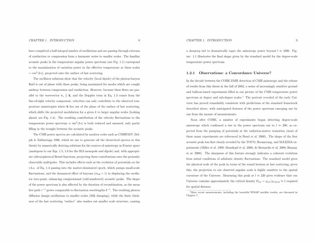
CHAPTER 1. INTRODUCTION 8
have completed a half-integral number of oscillations and are passing through extrema
of rarefaction or compression form a harmonic series to smaller scales. The familiar
acoustic peaks in the temperature angular power spectrum (see Fig. 1.1) correspond
to the maximization of variation power in the effective temperature at these scales
∼ cos2 (ks), projected onto the surface of last scattering.
The oscillator solutions show that the velocity (local dipole) of the photon-baryon
fluid is out of phase with these peaks, being maximized for modes which are caught
midway between compression and rarefaction. However, because these flows are par-
allel to the wavevector vγ ‖ k, and the Doppler term in Eq. 1.3 comes from the
line-of-sight velocity component, velocities can only contribute to the observed tem-
perature anisotropies where k lies out of the plane of the surface of last scattering,
which shifts the projected modulation for a given k to larger angular scales (looking
ahead, see Fig. 1.4). The resulting contribution of the velocity fluctuations to the
temperature power spectrum ∝ sin2 (ks) is both reduced and smeared, only partly
filling in the troughs between the acoustic peaks.
The CMB power spectra are calculated by modern codes such as CMBFAST (Sel-
jak & Zaldarriaga 1996, which we use to generate all the theoretical spectra in this
thesis) by numerically deriving solutions for the sources of anisotropy in Fourier space
(analogous to our Eqs. 1.5, 1.6 for the SLS monopole and dipole) and, with appropri-
ate (ultra)spherical Bessel functions, projecting these contributions onto the presently
observable multipoles. This includes effects such as the evolution of potentials on the
r.h.s. of Eq. 1.4 passing into the matter-dominated epoch, which pumps small-scale
fluctuations, and the dynamical effect of baryons (meff > 1) in displacing the oscilla-
tor zero-point, enhancing compressional (odd-numbered) acoustic peaks. The shape
of the power spectrum is also affected by the duration of recombination, as the mean
free path τ−1 grows comparable to fluctuation wavelengths k−1. The resulting photon
diffusion damps oscillations to smaller scales (Silk damping), while the finite thick-
ness of the last scattering “surface” also washes out smaller scale structure, causing
CHAPTER 1. INTRODUCTION 9
a damping tail to dramatically taper the anisotropy power beyond l ≈ 1000. Fig-
ure 1.1 illustrates the final shape given by the standard model for the degree-scale
temperature power spectrum.
1.2.1 Observations: a Concordance Universe?
In the decade between the COBE-DMR detection of CMB anisotropy and the release
of results from this thesis in the fall of 2002, a series of increasingly sensitive ground
and balloon-based experiments filled in our picture of the CMB temperature power
spectrum at degree and sub-degree scales.1 The portrait revealed of the early Uni-
verse has proved remarkably consistent with predictions of the standard framework
described above, with anticipated features of the power spectrum emerging one by
one from the mosaic of measurements.
Soon after COBE, a number of experiments began detecting degree-scale
anisotropy which confirmed a rise in the power spectrum out to l ≈ 200, as ex-
pected from the pumping of potentials at the radiation-matter transition (most of
these many experiments are referenced in Bond et al. 2000). The shape of the first
acoustic peak was first clearly revealed by the TOCO, Boomerang, and MAXIMA ex-
periments (Miller et al. 1999; Mauskopf et al. 2000; de Bernardis et al. 2000; Hanany
et al. 2000). The sharpness of this feature strongly indicates a coherent evolution
from initial conditions of adiabatic density fluctuations. The standard model gives
the physical scale of the peak in terms of the sound horizon at last scattering; given
this, the projection to our observed angular scale is highly sensitive to the spatial
curvature of the Universe. Measuring this peak at l ≈ 220 gives evidence that our
Universe contains approximately the critical density Ωtot = ρtot/ρcritical ≈ 1 required
for spatial flatness.
1More recent measurements, including the beautiful WMAP satellite results, are discussed inChapter 7.

CHAPTER 1. INTRODUCTION 10
0 200 400 600 800 1000 12000
1000
2000
3000
4000
5000
6000
7000
l(l+
1)/(
2π)
Cl
(µK
2 )
l (angular scale)
DASI 2001
Boomerang 2001
MAXIMA 2001
Figure 1.1 Measurements of the degree-scale CMB temperature power spectrum released at the
April 2001 American Physical Society meeting in Washington, DC. Shown are the DASI results
(Halverson et al. 2002) along with new analyses of the Boomerang (Netterfield et al. 2002) and
MAXIMA-1 (Lee et al. 2001) data (excluding beam and calibration uncertainties). The measure-
ments are in excellent agreement with each other and exhibit the acoustic peaks that are the expected
signature of adiabatic density perturbations under the standard CMB model. Theoretical spectra
calculated using this model with three different cosmological parameter combinations that fit this
data well are shown: the concordance model (solid green), a similar model with higher τ (dashed),
and a model with low h and high Ωm (dot-dashed). See text for details. (Figure adapted from
conclusion of Halverson (2002)).
CHAPTER 1. INTRODUCTION 11
In 2001, the acoustic interpretation of CMB physics received its strongest confir-
mation yet, with the detection of multiple acoustic peaks in the power spectrum out
to l ≈ 1000, revealed in measurements by the DASI telescope and new analyses by
Boomerang and MAXIMA (Halverson et al. 2002; Netterfield et al. 2002; Lee et al.
2001). These measurements (illustrated in Fig. 1.1) fit perfectly within the predictions
of the standard model, apparently tracking the evolution of the acoustic oscillations
through initial compression, rarefaction, and second compression with enough pre-
cision to fix most of the parameters of the model quite well. At even finer angular
scales, measurements by the CBI telescope traced the dissipation of power through
the damping tail (Pearson et al. 2002; Scott & et al. 2002), lending confidence to the
standard model account of recombination.
The power of these CMB temperature results to determine the cosmological pa-
rameters of the standard model is illustrated in Fig. 1.2, where we give parameter
constraints derived from the DASI measurements (Pryke et al. 2002). These con-
straints are derived by comparing the power observed by DASI in the nine bands
shown in Fig. 1.1 and at large scales by COBE against power spectra calculated for
a seven parameter model grid. The first four parameters define the composition and
expansion rate of the Universe, taken from combinations of the Hubble parameter h
(units of 100 km s−1 Mpc−1) and the present-day fraction of the critical density for
baryons Ωb, cold dark matter Ωcdm, and dark energy ΩΛ. Reionization, which can
suppress small-scale power by rescattering CMB photons at late times, is parameter-
ized by the optical depth τ to the SLS. Initial conditions are defined by the amplitude
and power-law index of the primordial adiabatic density (scalar) fluctuations, param-
eterized by C10 and ns.2 Of the seven major parameters we consider, Figure 1.2
shows that the CMB temperature data alone (with a weak h prior) offer a very good
2Two similar parameters can be added to specify the primordial tensor fluctuations discussed inthe next section. Inclusion of a running scalar index, a massive neutrino component, or a galaxybias parameter for large-scale structure comparisons, can bring the number of parameters to twelve,though these additional parameters are not needed to explain the degree-scale temperature spectrum.

CHAPTER 1. INTRODUCTION 12
−1 0 1 2 30
0.2
0.4
0.6
0.8
1
Ω∆≡ Ω
m− Ω
Λ
0.8 1 1.20
0.2
0.4
0.6
0.8
1
Ωtot
0.01 0.02 0.03 0.040
0.2
0.4
0.6
0.8
1
Ωbh2
0 0.1 0.2 0.3 0.40
0.2
0.4
0.6
0.8
1
Ωcdm
h2
0 0.1 0.2 0.3 0.40
0.2
0.4
0.6
0.8
1
τc
0.8 0.9 1 1.1 1.20
0.2
0.4
0.6
0.8
1
ns
400 600 800 1000 12000
0.2
0.4
0.6
0.8
1
C10
Figure 1.2 Cosmological parameter constraints from DASI temperature spectrum measurements.
Shown are marginal likelihood distributions for parameters of the standard model, derived for three
different priors on the Hubble parameter: no prior (dotted); a weak prior, h > 0.45 (solid); and a
strong prior, h = 0.72± 0.08 (dashed). Within the context of this model, degree scale CMB powerspectrum measurements provide good constraints on each of these parameters except τ and Ω∆.
The agreement of Ωbh2 with the independent Big Bang Nucleosynthesis (BBN) constraint (green)
is a crucial link between two pillars of observational cosmology (see text).
determination of five combinations.
The constraint on the physical baryon density Ωbh2 = 0.022+0.004−0.003, as described
above, comes from the influence ofmeff on the measured heights of the second acoustic
peak compared to the first and third. This result is remarkably consistent with the
Big Bang Nucleosynthesis (BBN) constraint Ωbh2 = 0.020 ± 0.001 derived from ob-
servations of primordial deuterium abundance (Burles et al. 2001). The concordance
of these two independent determinations of the baryon content of the Universe, one
involving nuclear physics in the first seconds of time, the other the acoustic dynamics
of the CMB, is a major victory for the standard model.
The cold dark matter density Ωcdmh2 = 0.14 ± 0.04 is also determined by the
CHAPTER 1. INTRODUCTION 13
heights of the first three peaks as they trace the evolution of potential wells into
the matter-domination epoch. The substantial height of the third peak is a direct
signature of this non-baryonic dark matter, present in the early Universe in a ∼7:1proportion to the baryons. This is consistent with the present-day dark matter content
inferred from numerous observations, including cluster gas mass fractions (Grego et al.
2001; Mohr et al. 1999) and various dynamical cluster estimates (see Turner 2002 for
a review).
Inflation makes three key predictions, two of which find support in this data. The
constraint Ωtot = Ωm+ΩΛ = 1.04± 0.06, which improved from previous estimates by
fixing the higher peaks, indicates the spatial curvature of the Universe is consistent
with the precise flatness expected from an early inflationary burst of expansion. The
spectral index ns = 1.01+0.08−0.06, measured across the broad range of scales probed by
COBE and DASI, confirms the approximate scale-invariance of the initial adiabatic
density fluctuations. The amplitude of these fluctuations given by C10 = 740 ± 100,
while not predicted by inflation theory, is at the correct level to explain the power
spectrum observed for present-day large scale structure (e.g. Wang et al. 2002).
The remaining parameters Ω∆ = Ωm − ΩΛ and τ are poorly constrained by the
CMB temperature data alone. However, because Ωtot and Ωmh2 are well-constrained,
the introduction of external information about either the total matter density Ωm
or the Hubble parameter h dramatically tightens the limits on Ω∆. For example,
including the HST Key project measurement h = 0.72± 0.08 yields Ωm = 0.40± 0.15
and ΩΛ = 0.60±0.15. This new measurement of the total matter density is consistent
with long-converging estimates from galaxy surveys (which probe Ωmh). However,
the implication that a dark energy component ΩΛ dynamically akin to Einstein’s
cosmological constant dominates the present-day Universe would have shocked many
(but not all, e.g. Krauss & Turner 1995), if not for recent results from high redshift
supernovae. Two teams have searched for type Ia SN to serve as standardizable
candles in tracking the recent expansion of the Universe, and have discovered an

CHAPTER 1. INTRODUCTION 14
acceleration of the expansion rate that indicates a dark energy component ΩΛ ∼Ωm + 0.3 (Perlmutter et al. 1999; Riess et al. 1998).
The fact that the standard model offers an excellent fit to the observed tempera-
ture power spectrum (Fig. 1.1) is a strong argument for the validity of its assumptions.
Each of the examples of concordance between cosmological parameters derived from
this fit and independent lines of evidence further strengthens the case. The solid
curve plotted in Fig. 1.1 is the CMBFAST-generated spectrum for what we will call
the concordance model : (Ωb, Ωcdm, ΩΛ, τ , ns, h, C10) = (0.05,0.35,0.60,0,1.00,0.65,700)
(Ostriker & Steinhardt 1995; Krauss & Turner 1995). Two other theoretical spectra
are shown to illustrate the two parameter combinations poorly-constrained by the
CMB data. A model with τ = 0.17 but otherwise similar parameters fits the data as
well as the concordance model.3 A model with Ω∆ = 0.4 is marginally the best fit
to the CMB data, but is less compatible with external measurements of h and Ωm.
The concordance model predicts the observed temperature spectrum very well, and
we will use it as a point of reference throughout this thesis.
While the striking convergence of theory and observation in the new standard
model of cosmology gives the impression of a solved problem, our concordance pic-
ture is actually a mosaic of unexplained, and in some cases unexpected mysteries.
Although inflation offers a beautiful explanation for the observed spatial flatness and
initial spectrum of adiabatic density fluctuations, this is only circumstantial evidence
which by itself has limited power to illuminate the mechanism, energy scale, or even
the certainty of the phenomenon. The apparent completeness of our account of the
composition of the Universe masks a shocking ignorance of the nature of each com-
ponent. Even the abundance of ordinary baryonic matter and its early origin in
matter-antimatter asymmetry lacks a theoretical explanation. The dark matter par-
ticle, the dominant form of matter in the Universe, remains unknown, and though
the CMB and local observations tell a consistent story of its abundance, questions
3This is the WMAPext preferred model discussed in Chapter 7
CHAPTER 1. INTRODUCTION 15
about its clustering dynamics persist. Most mysterious of all is the nature of the
dark energy, the dominant component of the present-day Universe. Interpreted as
the energy density of the vacuum state, field theory leads us to expect a value that
is either exactly zero due to cancellations or else ∼120 orders of magnitude greater
than observed (the “cosmological constant problem”). Moreover, the fact that Ωb
and Ωcdm are of the same order of magnitude is curious, but the fact that Ωm and ΩΛ
are comparable today is downright disturbing (the “coincidence problem”), because
this ratio evolves rapidly: ΩΛ/Ωm ∝ a−3w, where a is the expansion factor, and w
describes the dark energy equation of state (w = −1 for a cosmological constant,
w < −0.5 by current observations). Because of these two paradoxes, our current
picture of the cosmological mix of matter and dark energy has been described as a
“preposterous Universe” (Carroll 2001).
Much of our confidence in this current picture, and much of our hope for using
“precision cosmology” to unravel its mysteries, depends on our understanding of the
CMB. A direct test of the validity of standard model CMB physics would clearly be
useful.
1.3 CMB Polarization
The same acoustic oscillations that are central to our understanding of the temper-
ature power spectrum must also impart a polarization to the CMB (Kaiser 1983;
Bond & Efstathiou 1984; Polnarev 1985). Polarization therefore provides a model-
independent test of the acoustic paradigm on which our estimation of cosmological
parameters from the CMB depends (Hu et al. 1997; Kinney 2001; Bucher et al. 2001).
In addition, polarization measurements can in principle triple the number of observed
CMB quantities, promising eventually to improve those parameter estimates dramat-
ically (Zaldarriaga et al. 1997; Eisenstein et al. 1999).
For the two additional observables needed to describe CMB polarization, we can

CHAPTER 1. INTRODUCTION 16
Right Ascension
Dec
linat
ion
Temperature
−120’−60’0’60’120’
−120’
−60’
0’
60’
120’
−120’−60’0’60’120’
−120’
−60’
0’
60’
120’
Right Ascension
Dec
linat
ion
Pure E
−120’−60’0’60’120’
−120’
−60’
0’
60’
120’
Right Ascension
Dec
linat
ion
Pure B
Figure 1.3 CMB temperature and polarization maps are best understood in terms of independent
harmonic modes which reflect the underlying physics. Polarization maps can be decomposed into E
and B-type patterns in much the same way a vector field can be decomposed into gradient and curl
parts. A Fourier density mode (left) undergoing compression generates a pure E pattern (center),
in which polarization is aligned parallel or perpendicular to the direction of modulation. For the B
modes (right), polarization is ±45 to this direction. Together, the E and B harmonic modes form acomplete basis for polarization maps, just as conventional spherical harmonics (or on small patches
of sky, Fourier modes) form a basis for temperature maps.
choose the linear Stokes parameters Q and U measured at each point on the sky. (The
same information is represented by the polarization amplitude P =√Q2 + U 2 and
linear orientation α = 12arctanU/Q, typically depicted using headless polarization
“vectors”. No circular polarization V is expected.) Unlike T , the definition of Q and
U depend on the orientation χ of coordinate axes, transforming as spin-2 variables:
Q + iU → e−2iχ (Q+ iU). For this reason, the expression analogous to Eq. 1.1 that
gives the harmonic decomposition of polarization maps on the celestial sphere,
Q (x)± iU (x) =∑
l,m
−(aElm ± iaBlm
)±2Ylm (x) (1.7)
is written in terms of combinations of spin-2 spherical harmonics ±2Ylm (Newman &
Penrose 1966; Kamionkowski et al. 1997b; Zaldarriaga & Seljak 1997). Two distinct
sets of harmonic modes, called E and B-modes, correspond to the multipoles aElm
and aBlm and together form a complete basis for polarization maps. Their patterns
CHAPTER 1. INTRODUCTION 17
are easily visualized in the flat sky approximation, where E and B-modes are simply
Fourier modes of Q and U as defined in coordinates aligned with the 2-D wavevector u
(Seljak 1997). Thus, for E-modes the polarization is aligned parallel or perpendicular
to the direction of modulation, while for B-modes it is at ±45 (Figure 1.3).
The polarization power spectra are defined
CEl =
⟨aElm
∗aElm⟩
CBl =
⟨aBlm
∗aBlm⟩, (1.8)
just as we defined the temperature spectrum (henceforth CTl ) in Eq. 1.2. There are
also three possible cross-spectra
CTEl =
⟨aTlm
∗aElm⟩
CTBl =
⟨aTlm
∗aBlm⟩
CEBl =
⟨aElm
∗aBlm⟩, (1.9)
however, because theB-modes have opposite parity from E and T , parity conservation
demands the last two of these to vanish. Assuming Gaussian fluctuations, the T , E,
B, and TE spectra specify the complete statistics of the CMB temperature and
polarization fields.
In contrast to the temperature anisotropies, CMB polarization arises from a single
mechanism: the effect of a local quadrupole in the intensity of CMB photons at the
point of their last scattering (Rees 1968). The Thompson scattering cross section σT
has a directional dependence (e.g. Chandrasekhar 1960)
dσ
dΩ=
3
8π|εin · εout| σT (1.10)
on the incoming and outgoing polarization orientation. Because εin must be trans-
verse, a free electron which “sees” a randomly polarized incident photon field with
any ± cos2 θ intensity variation will scatter those photons with an outgoing net linear
polarization perpendicular (parallel) to this “hot” (“cold”) quadrupole axis.
In the primordial plasma, rapid rescattering initially suppresses the local
quadrupole, keeping the photon field randomly polarized and isotropic in the rest
frame of the electrons. As recombination proceeds, the rapid growth of the mean free

CHAPTER 1. INTRODUCTION 18
path τ−1 allows the local photon field to probe spatial variations; the second-to-last
scattering sets the conditions that generate the final polarization. Acoustic density
oscillations create a local quadrupole from the spatial gradient of the local photon
dipole vγ, which is essentially the Doppler shift due to the photon-baryon velocity
field (but as tight coupling breaks down also accounts for photon diffusion from hotter
regions). For a spatial Fourier mode, the quadrupole amplitude is (Kaiser 1983)
qγ,k =32
15
k
τvγ,k. (1.11)
This equation explains the shape and height of the polarization spectrum (Hu 2003).
The factor of k/τ reflects the fact that the local quadrupole probes the gradient in
vγ,k on scales of the mean free path. Consequently, the polarization power (∝ q2) rises
at large scales as l2 and peaks near the damping scale ld ≈ 1000 at a level roughly
(kd/τ)2 ∼ (1/10)2 the temperature power. At smaller scales, the diffusion damping
of the acoustic source vγ,k dominates, producing a damping tail similar to that of the
temperature spectrum.
The pattern of CMB polarization generated by an acoustic oscillation is illustrated
in Fig. 1.4. A spatial Fourier mode of wavevector k initially undergoes compression,
the photon-baryon fluid flowing vγ ‖ k from effectively hot crests to cold troughs.
The gradient in photon flow produces anm = 0 quadrupole in the local radiation field
seen from troughs (or crests), with the hot (cold) axis parallel to the wavevector. The
resulting polarization pattern in the surface of last scattering is like Fig. 1.3 (center),
a pure E-mode. During the rarefaction phase the reversal of flows exchanges hot and
cold, swapping the sign of the E-mode. Where the wavevector k is not perpendicular
to our line of sight, the projected angular scale of the modulation is increased, and
the amplitude of the polarization decreases as the square of the projected length of
the hot (cold) quadrupole axis onto the SLS. The orientation is always parallel or
perpendicular to kproj, the only direction in the problem; density oscillations cannot
generate B-mode polarization.
CHAPTER 1. INTRODUCTION 19
Figure 1.4 CMB polarization is directly generated by the acoustic oscillations during last scattering.
As the spatial Fourier mode undergoes compression, the flow of photons vγ from effectively hot
crests toward effectively cold troughs produces an m = 0 quadrupole in the local radiation field
seen from troughs (or crests), with the hot (cold) axis parallel to k. This produces a pattern of
linear polarization in the surface of last scattering (dotted frame) which alternates perpendicular
and parallel to the projected wavevector. The angle with which k intersects the last scattering
surface changes the projected scale of the modulation (left vs. right), but the pattern can only be
E-mode (figure inspired by Hu & White 1997).
Since the velocities at last scattering are the source of this CMB polarization
qγ,k ∝ vγ,k, the acoustic peak structure of the E spectrum captures the evolution of
these velocities on different scales. Our oscillator solutions Eqs. 1.5 and 1.6 showed
that while the effective temperature traces a cos (ks) evolution, the velocities evolve
as sin (ks), being maximized for modes which are caught midway between extreme
compression and rarefaction. It is evident that the peaks in the E spectrum, with
a ∼ sin2 (ks) character, will be approximately 180 degrees out of phase from the
temperature peaks (∼ cos2 (ks)). The same is true of the Doppler contribution that
partially fills the valleys of the temperature spectrum, but because the polarization is
generated by transverse velocities vγ ⊥ x, its projection is a sharp function of angular
scale. For this reason, the peaks in the E spectrum are more pronounced than those
in the T spectrum (Fig. 1.6), and they offer a specific probe of the dynamics at the

CHAPTER 1. INTRODUCTION 20
Figure 1.5 Tensor oscillations (gravity waves) present at last scattering could also contribute to
CMB polarization. The transverse contraction/expansion of a standing gravity wave generates an
m = 2 quadrupole in the local radiation field. Viewed edge-on (k ⊥ x), a gravity wave with +
polarization projects one of its quadrupole axes onto the SLS (dotted frame), producing an E-mode
pattern (left), while for a × wave the two axes cancel, giving no net polarization (not shown).
However, when k intersects the SLS at an angle, both quadrupole axes of the × wave contribute toa net polarization on the SLS that is ±45 to kproj, producing a B-mode pattern (right).
epoch of decoupling (Zaldarriaga & Harari 1995).
It is clear that the CMB temperature and polarization anisotropy should be corre-
lated at some level, because they are sourced by the same oscillations (Coulson et al.
1994). The spectrum of the TE correlation has roughly a sin (ks) cos (ks) character,
reflecting the fact that for a given mode, the sign of the generated E-mode reverses
when the flow switches between compression and rarefaction, while the sign of the
temperature signal reverses midway between these extrema. Zero crossings of the
predicted TE spectrum, illustrated in Fig. 1.6, occur at the nulls of both the E and
the T spectra. This unique signature in TE offers a powerful test of the underlying
acoustic paradigm.
The acoustic oscillations come from primordial fluctuations in the curvature, or
CHAPTER 1. INTRODUCTION 21
scalar component of the metric. Tensor metric perturbations, if present at last scat-
tering, could also contribute to the CMB polarization (Polnarev 1985; Crittenden
et al. 1993). Inflationary expansion generates a primordial spectrum of tensor per-
turbations which can be viewed as standing gravity waves. The time evolution of the
familiar gravity wave contraction/expansion transverse to k will redshift or blueshift
photons in proportion to their mean free time-of-flight, producing an m = 2 local
quadrupole. (Vector perturbations will produce an m = 1 quadrupole, but being
suppressed by expansion these are not expected.) Figure 1.5 illustrates how the
intrinsic polarization of the gravity waves with respect to the surface of last scatter-
ing leads to the generation of both E and B-mode CMB polarization (Seljak 1997;
Kamionkowski et al. 1997a; Seljak & Zaldarriaga 1997). The tensor E spectrum will
be unobservable, swamped by the much stronger scalar signal. The B modes are
only generated by × gravity waves where k lies out of the plane of the SLS, so that
similar to the Doppler T contribution, the tensor B spectrum is reduced compared
to the tensor E spectrum,4 with its features smeared and somewhat shifted to larger
angular scales (see Fig. 1.6). The gravity waves oscillate coherently at a frequency
ck ≈√3csk, so peaks in the tensor spectra occur with spacing that is 1/
√3 that of
the acoustic peaks. Because the strength of the tensor quadrupole depends on the
oscillation frequency and mean free path q ∝ k/τ , the tensor polarization spectra rise
like the scalar E spectrum, as ∼ l2 at large scales. However, like all radiation, gravity
waves decay upon entering the horizon, so the tensor spectra peak at the horizon
scale l ∼ 100 and at smaller scales are rapidly damped.
The production of primordial gravity waves is the last and most distinctive of
the three key predictions of inflation mentioned in the previous section. Detection of
the B-spectrum of polarization arising from these inflationary gravity waves would
be a monumental achievement for the CMB; not only would it be “smoking gun”
evidence that inflation occurred, but the energy scale and evolution of the process
4The actual ratio 8/13 is related to Clebsh-Gordan coefficients (Hu & White 1997).

CHAPTER 1. INTRODUCTION 22
10−2
100
102
T
E
Bgravity waves
density oscillations
lensing
2 50 200 400 600 800 1000 1200 1400
−100
0
100
TE
l(l+
1) /
(2π)
Cl
(µK
2 )
l (angular scale)
Figure 1.6 Standard model predictions for the CMB temperature and polarization power spec-
tra. The temperature (T) and E-mode polarization (E) spectra are dominated by the dynamics
of the acoustic oscillations, with a relationship encoded in their cross correlation spectrum (TE).
Late-time distortion of E-modes by gravitational lensing produces a predictable level of B polariza-
tion (dot-dash), while the level of intrinsic E and B from primordial gravity waves (dashed lines)
depends on the highly uncertain energy scale of inflation. The effect of early reionization (τ = 0.17)
on each spectrum is shown by dotted lines at large scales. See text for details.
CHAPTER 1. INTRODUCTION 23
would be directly revealed in the level and slope of the tensor spectrum. Unfortu-
nately, theory offers few lower limits on this level (e.g. Lyth 1997). Furthermore, the
late-time distortion of E-modes by gravitational lensing from large scale structure
also produces B polarization, with an envelope that roughly traces the shape of the
E spectrum (Zaldarriaga & Seljak 1998). The detailed mapping of these lensing B
modes could allow separation of a tensor B signal down to a minimum detectable
inflationary energy scale of ∼ 1015 GeV (Hu & Okamoto 2002; Knox & Song 2002;
Kesden et al. 2002). Mapping the lensing B signal will also allow accurate recon-
struction of the lensing potential field, offering a powerful probe of the dark matter-
and dark energy-dependent growth of structure. Possible applications include con-
straining the neutrino mass (Kaplinghat et al. 2003) or using cross-correlation with
the ISW effect to test properties of the dark energy (Hu 2002).
These faint B-mode polarization signals, which could extend the reach of the
standard model to physics at the earliest and latest times, are observational targets
for the future. First, measurements of the predicted E and TE spectra will offer
many opportunities to test and refine the core assumptions of the standard model.
For example, observation of a peak in the E and TE spectra at large scales would
be evidence of rescattering of CMB photons by early reionization (see Fig. 1.6, also
Chapter 7). Comparison of the acoustic peaks of the E and T spectra allow precise
constraints on isocurvature fluctuations or primordial spectrum features, the effects
of which could be degenerate with cosmological parameters in the T spectrum alone.
Detailed measurement of the shape of the E spectrum, which is sensitive to the
way in which recombination occurred, will strictly limit the variation of fundamental
constants (α, G), processes that would inject additional ionizing photons, or depar-
tures from the standard expansion history. For a review of these and other tests, see
Zaldarriaga 2003.
Naturally, the first goal for experiments is the detection of CMB polarization, and
the determination whether it has the level and E-mode character predicted by the

CHAPTER 1. INTRODUCTION 24
standard model.
1.3.1 Searching for Polarization
The very low level of the expected CMB polarization signal, which peaks at . 1% of
the power in the T spectrum, presents a great experimental challenge. As progress
has been made in both sensitivity and control over systematic effects, from the earliest
days of CMB measurements a series of careful experiments have achieved increasingly
tight upper limits on the level of CMB polarization (see Staggs et al. 1999, for a review
of CMB polarization measurements).
Penzias and Wilson set the first limit to the degree of polarization of the CMB
in 1965, reporting that the new radiation they had discovered was isotropic and
unpolarized within the limits of their observations (Penzias & Wilson 1965). Over the
next 20 years, groups in Princeton, Italy, and Berkeley used dedicated polarimeters
to set much more stringent upper limits at angular scales larger than several degrees
(Caderni et al. 1978; Nanos 1979; Lubin & Smoot 1979, 1981; Lubin et al. 1983,
see also Sironi et al. 1997). Although the focus of the COBE/DMR experiment
was detecting the large scale temperature anisotropy, it also constrained the level
of polarization at these scales (Smoot 1999). In 2001, the POLAR experiment set
the best upper limits for E-mode and B-mode polarization at large angular scales,
limiting these to 10 µK at 95% confidence for the multipole range 2 ≤ l ≤ 20 (Keating
et al. 2001).
At degree angular scales, the first limit to CMB polarization came from the
Saskatoon experiment in 1993; during observations which detected temperature
anisotropies at these scales, a constraint was placed on polarization (25 µK at 95%
confidence for l ∼ 75) which was the first reported limit lower than the level of the
temperature signal. The best limit on similar angular scales was set by the PIQUE
experiment (Hedman et al. 2002) — a 95% confidence upper limit of 8.4 µK to the
E-mode signal, assuming no B-mode polarization. Analysis of polarization data from
CHAPTER 1. INTRODUCTION 25
10 100 100010
−2
100
102
104
106
108
1010
POLAR 01 PIQUE 02
SASK 93
Lubin/Smoot 79
Lubin/Smoot 81,83
Caderni 78Nanos 79
DMR 99
MILANO 99
CBI 02
Penzias/Wilson 65
l(l+
1)/(
2π)
Cl
(µK
2 )
l (angular scale)
Figure 1.7 Increasingly tight experimental limits to the level of CMB polarization prior to the 2002
DASI detection. For reference, the expected level of E polarization is shown for the concordance
model (solid green) and for τ = 0.17 (dashed). The level of the temperature anisotropies is also
shown (faint gray). See text for experimental references.

CHAPTER 1. INTRODUCTION 26
the Cosmic Background Interferometer (CBI) (Cartwright 2003) indicates upper lim-
its similar to the PIQUE result, but on smaller scales. An attempt was also made to
search for the TE correlation using the PIQUE polarization and Saskatoon temper-
ature data (de Oliveira-Costa et al. 2003b).
Polarization measurements have also been pursued at much finer angular scales
(of order an arcminute), resulting in several upper limits (e.g. Partridge et al. 1997;
Subrahmanyan et al. 2000). These measurements, like those of the CBI, are no-
table for employing interferometry in the pursuit of CMB polarization. However,
at these angular scales, corresponding to multipoles ∼ 5000, the primary sources of
CMB temperature and polarization anisotropy are strongly damped, and secondary
anisotropies or foregrounds are expected to dominate (Hu & Dodelson 2002).
1.4 The Degree Angular Scale Interferometer
The Degree Angular Scale Interferometer (DASI) was conceived as an instrument
that would take advantage of newly available low-noise HEMT amplifiers to combine
interferometry with the appropriate sensitivity and angular resolution to explore the
CMB power spectra in the region of the acoustic peaks. It would share many back-
end components with the CBI, a sister instrument to be developed at Caltech, which
would pursue CMB measurements at smaller angular scales. Lead by John Carlstrom,
work began on DASI at the University of Chicago in 1996. Early DASI publications
chronicle the design of the instrument (e.g. Halverson et al. 1998) and theory of
interferometric sensitivity to the CMB (White et al. 1999a,b).
DASI was shipped to the National Science Foundation Amundsen-Scott South
Pole research station in November 1999, and in early 2000 began observations of CMB
temperature anisotropy which continued throughout the following austral winter. The
results of this first season, some of which have already been discussed, were released
at the April 2001 APS meeting in Washington, DC, and presented in a series of three
CHAPTER 1. INTRODUCTION 27
papers, published together (Leitch et al. 2002b; Halverson et al. 2002; Pryke et al.
2002, hereafter, Papers I, II and III, respectively). Paper I details the design of the
instrument and observations, and includes maps of the 32 fields, each 3.4 FWHM,
in which temperature anisotropies were measured. Paper II presents the analysis
and power spectrum results which revealed the presence of multiple acoustic peaks in
the T spectrum (Fig. 1.1). Paper III gives the constraints obtained on cosmological
parameters from these measurements (Fig. 1.2). The temperature observation results
of Papers I-III are further detailed in the doctoral thesis of N. Halverson (2002).
1.4.1 Plan of this Thesis
Prior to the start of the 2001 season, DASI was modified to allow polarization mea-
surements in all four Stokes parameters over the same l range as the previous measure-
ments. Polarization data were obtained within two 3.4 FWHM fields during the 2001
and 2002 austral winter seasons, and analysis of the data proceeded simultaneously
with the observations. In September 2002, the results of this work were presented at
the Cosmo-02 workshop in Chicago, IL. The E-mode polarization of the CMB was
detected at high confidence (≥ 4.9σ). The level was found to be consistent with the
E spectrum predicted to arise from acoustic oscillations due to primordial adiabatic
scalar fluctuations under the standard model. No significant B-mode polarization was
observed. The TE correlation of the temperature and E-mode polarization was de-
tected at 95% confidence and also found to be consistent with predictions. This work
was reported in two papers, published together. The modifications to the instrument,
observational strategy, calibration and reduction of the polarization observations were
presented in Paper IV (Leitch et al. 2002a). The data analysis and CMB polarization
results were reported in Paper V (Kovac et al. 2002).
This thesis describes the DASI polarization measurements, from experimental de-
sign to final results. It incorporates all of the material that appeared in Paper V and

CHAPTER 1. INTRODUCTION 28
much of that of Paper IV, especially within Chapters 4–6. The emphasis and orga-
nization of this thesis reflect the specific contributions of the author, which include
the construction of the sensitivity-defining amplifiers and polarizers, the design of the
polarization observing and calibration strategies, and the data analysis and likelihood
results. Virtually every aspect of DASI, including these, has been the product of an
extraordinary collaboration. The acknowledgments section and some notes in the text
attempt to identify obvious contributions of other team members, but the production
of Papers IV and V was essentially a team effort, and the use of the first person plural
throughout this thesis is intended to acknowledge the DASI team—J. E. Carlstrom,
M. Dragovan, N. W. Halverson, W. L. Holzapfel, J. M. Kovac, E. Leitch, C. Pryke,
B. Reddall, and E. Sandberg—who are the co-authors of these results.
Beginning in Chapter 2, we discuss some advantages of interferometric observa-
tions of the CMB, emphasizing the match between the Fourier sky response pattern of
a polarized interferometer and the E and B-mode patterns illustrated in Fig. 1.3. We
also develop much of the formalism which we later apply in the analysis. Chapter 3
gives a brief overview of the DASI instrument and describes in some detail the HEMT
amplifiers and the achromatic circular polarizers which were developed to give DASI
precise polarization sensitivity. In Chapter 4, the actual polarization response of the
instrument is verified, calibrated, and modeled using a number of dedicated obser-
vations. The CMB observations are discussed in Chapter 5, and the critical steps of
data reduction, noise modeling, and consistency tests described. This chapter ends
with the identification of a polarized signal in the CMB data, visibly apparent in a
polarization map. Chapter 6 presents the method and results of the likelihood analy-
ses which test the properties of the observed polarized signal, comparing it to various
predictions of the standard model. Finally, in Chapter 7 we discuss these results,
considering the statistical confidence of detection and the degree to which predictions
of the standard model have been tested, and we conclude with a look ahead to new
measurements and future directions for CMB polarization.
Chapter 2
Interferometric CMB measurement
The first attempts to use interferometry as a technique for measuring temperature
and polarization variations of the CMB were made using existing large radio telescope
arrays. While work by groups at the VLA (e.g. Fomalont et al. 1984; Partridge
et al. 1988), ATCA (Subrahmanyan et al. 1993), and Ryle (Jones 1997) facilities
produced upper limits at the very small angular scales accessible to these arrays,
prototype compact instruments were developed to operate at angular scales more
suited to the expected CMB signal (see White et al. (1999a) for complete references).
The advent of low-noise, broadband, millimeter-wave HEMT amplifiers (Pospieszalski
et al. 1994) enabled the development of the modern generation of high-sensitivity
CMB interferometers, designed specifically to measure the CMB power spectra on
angular scales of interest. In addition to DASI and its sister experiment the CBI, these
purpose-built CMB interferometers include the VSA (Jones 1996) and the upcoming
AMiBA experiment (Lo et al. 2001).
Interferometry has many attractive features for ground-based CMBmeasurements.
Because they directly sample Fourier components of the sky, interferometers are well
suited to measurements of the CMB angular power spectrum. Their angular sensi-
tivity depends on array geometry rather than optical beam properties, offering an
extremely stable and well-characterized sky response. This two dimensional response
pattern is sampled instantaneously while inherently rejecting large-scale gradients in
29

CHAPTER 2. INTERFEROMETRIC CMB MEASUREMENT 30
atmospheric emission. Multiple levels of fast phase switching, made possible by coher-
ent amplification, downconversion and correlation, combine to offer superb rejection
of instrumental offsets.
For observations of CMB polarization, interferometers offer several additional ad-
vantages. They can be constructed with compact, symmetrical optics that have small
and stable instrumental polarization. Furthermore, linear combinations can be con-
structed from their direct output which are essentially pure E- and B-mode polariza-
tion response patterns on a variety of scales, closely matching the patterns illustrated
in Fig. 1.3. This property of the data greatly facilitates the analysis and interpreta-
tion of the observed polarization in the context of the anticipated CMB polarization
signals.
In the next two chapters, we will discuss ways in which DASI’s instrumental
design attempts to take full advantage of these features offered by interferometry. Our
focus in this chapter will be DASI’s theoretical response to the CMB as a polarized
interferometer. First we will derive the polarized sky response pattern for a single
pair of receivers and examine the natural separation of E and B-mode polarization
that it offers. Next we calculate the theory covariance matrix, which describes the
statistical response of the complete dataset to the CMB power spectra. This matrix
will become a basic tool of our analysis in Chapter 6. We conclude with a simple
application of this matrix, as we discuss DASI’s expected level of sensitivity to the
polarization power spectra.
2.1 Polarized Visibility Response
The basic output of DASI’s complex correlator is the visibility, a time-averaged cross-
correlation of the electric fields measured by each pair of receivers in the array. To
derive the response of the visibility to polarized sky signals, we begin by considering
CHAPTER 2. INTERFEROMETRIC CMB MEASUREMENT 31
Figure 2.1 Schematic representation a single baseline u of an interferometer. An incident
plane-wave signal has orthogonal electrical field components E1 and E2, which arrive at the re-
ceivers with relative path difference λu · x. The focusing optics sample the electric field distributionacross the aperture of each receiver, defining the directional sensitivity. The polarizing optics define
the linear combination of field components (ErxA ∝ α1E1 + α2E2) that is amplified and passed to
the complex correlator.
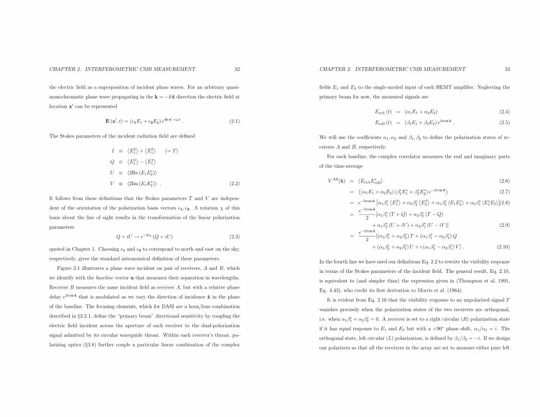
CHAPTER 2. INTERFEROMETRIC CMB MEASUREMENT 32
the electric field as a superposition of incident plane waves. For an arbitrary quasi-
monochromatic plane wave propagating in the k = −kx direction the electric field at
location x′ can be represented
E (x′, t) = (ε1E1 + ε2E2) eik·x′−iωt . (2.1)
The Stokes parameters of the incident radiation field are defined
I ≡⟨E21
⟩+⟨E21
⟩(= T )
Q ≡⟨E21
⟩−⟨E21
⟩
U ≡ 〈2Re (E1E∗2)〉
V ≡ 〈2Im (E1E∗2)〉 . (2.2)
It follows from these definitions that the Stokes parameters T and V are indepen-
dent of the orientation of the polarization basis vectors ε1, ε2. A rotation χ of this
basis about the line of sight results in the transformation of the linear polarization
parameters
Q+ iU → e−2iχ (Q+ iU) (2.3)
quoted in Chapter 1. Choosing ε1 and ε2 to correspond to north and east on the sky,
respectively, gives the standard astronomical definition of these parameters.
Figure 2.1 illustrates a plane wave incident on pair of receivers, A and B, which
we identify with the baseline vector u that measures their separation in wavelengths.
Receiver B measures the same incident field as receiver A, but with a relative phase
delay e2πiu·x that is modulated as we vary the direction of incidence x in the plane
of the baseline. The focusing elements, which for DASI are a horn/lens combination
described in §3.2.1, define the “primary beam” directional sensitivity by coupling the
electric field incident across the aperture of each receiver to the dual-polarization
signal admitted by its circular waveguide throat. Within each receiver’s throat, po-
larizing optics (§3.8) further couple a particular linear combination of the complex
CHAPTER 2. INTERFEROMETRIC CMB MEASUREMENT 33
fields E1 and E2 to the single-moded input of each HEMT amplifier. Neglecting the
primary beam for now, the measured signals are
ErxA (t) = (α1E1 + α2E2) (2.4)
ErxB (t) = (β1E1 + β2E2) e2πiu·x . (2.5)
We will use the coefficients α1, α2 and β1, β2 to define the polarization states of re-
ceivers A and B, respectively.
For each baseline, the complex correlator measures the real and imaginary parts
of the time-average
V AB(x) = 〈ErxAE∗rxB〉 (2.6)
=⟨(α1E1 + α2E2) (β
∗1E
∗1 + β∗
2E∗2) e
−2πiu·x⟩
(2.7)
= e−2πiu·x[α1β
∗1
⟨E21
⟩+ α2β
∗2
⟨E22
⟩+ α1β
∗2 〈E1E
∗2〉+ α2β
∗1 〈E∗
1E2〉](2.8)
=e−2πiu·x
2[α1β
∗1 (T +Q) + α2β
∗2 (T −Q)
+ α1β∗2 (U + iV ) + α2β
∗1 (U − iV )] (2.9)
=e−2πiu·x
2[(α1β
∗1 + α2β
∗2)T + (α1β
∗1 − α2β∗
2)Q
+ (α1β∗2 + α2β
∗1)U + i (α1β
∗2 − α2β∗
1)V ] . (2.10)
In the fourth line we have used our definitions Eq. 2.2 to rewrite the visibility response
in terms of the Stokes parameters of the incident field. The general result, Eq. 2.10,
is equivalent to (and simpler than) the expression given in (Thompson et al. 1991,
Eq. 4.43), who credit its first derivation to Morris et al. (1964).
It is evident from Eq. 2.10 that the visibility response to an unpolarized signal T
vanishes precisely when the polarization states of the two receivers are orthogonal,
i.e. when α1β∗1 +α2β
∗2 = 0. A receiver is set to a right circular (R) polarization state
if it has equal response to E1 and E2 but with a +90 phase shift, α1/α2 = i. The
orthogonal state, left circular (L) polarization, is defined by β1/β2 = −i. If we designour polarizers so that all the receivers in the array are set to measure either pure left

CHAPTER 2. INTERFEROMETRIC CMB MEASUREMENT 34
or pure right circular polarization, Eq. 2.10 gives the four possible combinations
V RR(x) = [T + V ] e−2πiu·x
V LL(x) = [T − V ] e−2πiu·x
V RL(x) = [Q+ iU ] e−2πiu·x
V LR(x) = [Q− iU ] e−2πiu·x . (2.11)
Recovery of the full set of Stokes parameters for a given baseline requires the meas-
urement of all four pairwise combinations of left and right circular polarization states
(RR, LL, RL and LR), which we refer to as Stokes states. The co-polar states (RR,
LL), are sensitive to the total intensity (and any incident net circular polarization),
while the cross-polar states (RL, LR) measure linear polarization. The potential for
residual total intensity response in the cross-polar visibilities due to leakage of the
unwanted circular polarization state is discussed in §4.4; for the present, we assume
ideal polarizers.
To obtain the full expression for the visibilities observed for a given baseline ui, we
must integrate the plane-wave visibility response of Eqs. 2.11 over the field of view,
V RR (ui) = αi
∫dx A (x, νi) [T (x) + V (x)] e−2πiui·x
V LL (ui) = αi
∫dx A (x, νi) [T (x)− V (x)] e−2πiui·x
V RL (ui) = αi
∫dx A (x, νi) [Q (x) + iU (x)] e−2πiui·x
V LR (ui) = αi
∫dx A (x, νi) [Q (x)− iU (x)] e−2πiui·x, (2.12)
where A (x, νi) specifies the primary beam power pattern at frequency νi, T (x),
Q(x), U(x), and V (x) are specified in units of CMB temperature (µK), and
αi = ∂BPlanck (νi, TCMB) /∂T is the appropriate factor for converting from these units
to flux density (Jy). Here we have assumed that the aperture field distributions of
both receivers are identical and independent of polarization, so that the primary beam
CHAPTER 2. INTERFEROMETRIC CMB MEASUREMENT 35
Right Ascension
Dec
linat
ion
Real(RR) , Real(LL)
180’ 120’ 60’ 0’ −60’ −120’ −180’
−180’
−120’
−60’
0’
60’
120’
180’
−120’−60’0’60’120’
−120’
−60’
0’
60’
120’
Right Ascension
Dec
linat
ion
Real(RL)
−120’−60’0’60’120’
−120’
−60’
0’
60’
120’
Right Ascension
Dec
linat
ion
Real(LR)
Figure 2.2 The fringe pattern of the co-polar visibility response (real part) to temperature is shown
at left for one of DASI’s shortest baselines (u = 30), oriented horizontally. RR and LL Stokes states
have identical response to T . The analogous cross-polar response is to linear polarization is shown
for RL and LR at right. Moving across the corrugation pattern, the change in relative phase delay
combines with the Q± iU response to cause a rotation of the plane of linear polarization response.
The sense of the rotation is opposite for RL and LR.
A(x, ν) simply corresponds to the Fourier transform of the aperture field autocorrela-
tion measured in wavelengths. Residual polarization dependence can produce off-axis
leakage, considered in §4.5. In principle, the response should also be integrated over
the finite correlated bandwidth ∆ν, to account for the delay beam destructive inter-
ference of the fringes e−2πiui·x many cycles from phase center that is caused by the
scaling |ui| ∝ ν. However, for DASI the fractional correlated bandwidth (1 GHz /
∼ 30 GHz) is small enough compared to the ratio of the aperture diameter to the
longest baseline ( 24 λ / 143 λ) that the primary beam dominates the delay beam,
which can be neglected except for calculation of interfield correlations.
The sky response patterns that correspond to the integrands of Eq. 2.12 are illus-
trated in Fig. 2.2. The gradient in the phase term e−2πiui·x across the main beam in
the direction parallel to the baseline results in a corrugation which, for the real part
of the co-polar visibilities, gives a simple positive-negative fringe pattern. The same
phase term modulating the Q + iU response of the RL visibility rotates the plane

CHAPTER 2. INTERFEROMETRIC CMB MEASUREMENT 36
−120’−60’0’60’120’
−120’
−60’
0’
60’
120’
Right Ascension
Dec
linat
ion
Real(RL + LR)
−120’−60’0’60’120’
−120’
−60’
0’
60’
120’
Right Ascension
Dec
linat
ion
Real(RL − LR)
Figure 2.3 Linear combinations of the cross-polar visibilities RL and LR give nearly pure E and
B-mode response patterns (compare Fig. 1.3). For a horizontal baseline, the E and B combinations
result from simply adding and subtracting the patterns in Fig. 2.2. These patterns deviate from
pure E or B only in the taper of the primary beam; for longer baselines the modulation scale is
small compared to the primary beam, and the purity of the E/B separation becomes nearly perfect.
of linear polarization response, as in Eq. 2.3, at half the fringe rate. The Q − iU
response of the LR visibility is rotated by the phase gradient in the opposite sense.
It is apparent from Eq. 2.12 that the observed visibilities are closely related to
the Fourier transform of the sky distribution of T , Q, and U—in fact, that if the pri-
mary beam A(x) were sufficiently broad, they would directly measure combinations
of the Fourier mode u of these fields. In Chapter 1 we stated that in the flat-sky
approximation, the E and B-modes are simply Fourier modes of Q and U as defined
in coordinates rotated (using Eq. 2.3) to align with u. Thus, as illustrated in Fig. 2.3,
the separation of Q and U that comes from forming the combinations RL+ LR and
RL − LR offers, for a horizontal baseline, a nearly pure separation of the Fourier
modes E(u) and E(u). For baselines of other orientations, a combination with an ap-
propriate phase rotation accomplishes the same separation. Because interferometers
directly measure nearly pure T , E and B Fourier modes on the sky, the data they
produce easily lends itself to placing independent constraints on these power spectra.
CHAPTER 2. INTERFEROMETRIC CMB MEASUREMENT 37
2.1.1 CMB Response and the uv-Plane
So far, we have emphasized the interferometric response pattern in the sky plane. It
is common practice in interferometry analysis to work mainly in the Fourier, or uv-
plane. This approach is especially suited to analyzing response to the CMB, because
in the flat sky approximation, the expected signal consists of uncorrelated Fourier
modes.
The flat sky formalism offers an accurate description of CMB statistics within
DASI’s 3.4 field of view (White et al. 1999a). In this approximation, the temperature
power spectrum is defined
CTl ' CT (u) ≡
⟨T ∗(u) T (u)
⟩, (2.13)
where T (u) is the Fourier transform of T (x) and l/2π = |u| gives the correspondencebetween multipole l and Fourier radius u = |u|. The variance of the uncorrelated
multipoles alm has been replaced by that of independent Fourier modes. The flat sky
polarization spectra and cross spectra are similarly defined,
CE (u) ≡⟨E∗(u) E (u)
⟩CB (u) ≡
⟨B∗(u) B (u)
⟩(2.14)
CTE (u) ≡⟨T ∗(u) E (u)
⟩CTB (u) ≡
⟨T ∗(u) B (u)
⟩CEB (u) ≡
⟨E∗(u) B (u)
⟩
The correspondence we have described between the Fourier modes of E,B and those
of Q,U can be written
Q (u) = cos (2χ) E (u)− sin (2χ) B (u)
U (u) = sin (2χ) E (u) + cos (2χ) B (u) , (2.15)
where the uv-plane azimuthal angle χ = arg(u) and the polarization orientation angle
defining Q,U are both measured on the sky from north through east. Note that unlike
in the sky plane, this transformation is strictly local in the uv-plane. Because T , Q, U
are Fourier transforms of real fields, conjugate points on the uv-plane are associated,
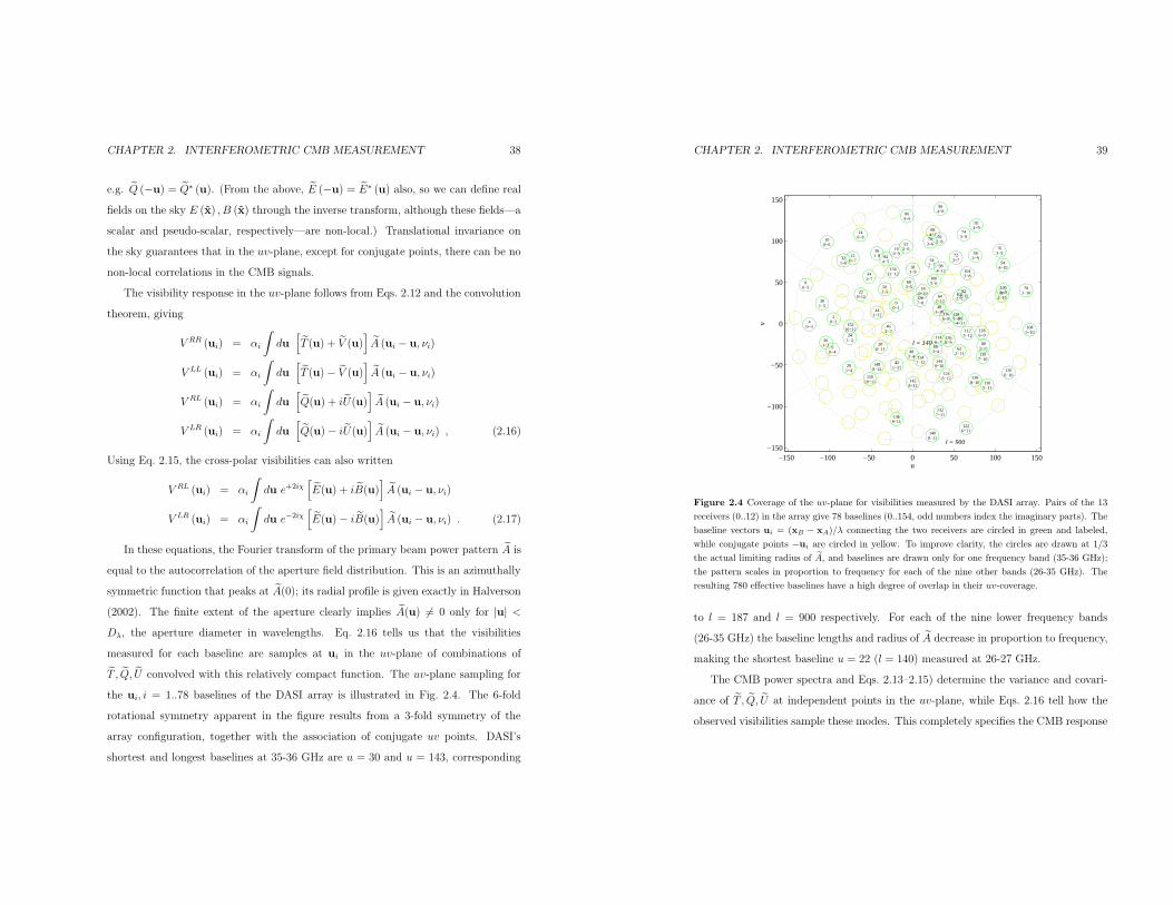
CHAPTER 2. INTERFEROMETRIC CMB MEASUREMENT 38
e.g. Q (−u) = Q∗ (u). (From the above, E (−u) = E∗ (u) also, so we can define real
fields on the sky E (x) , B (x) through the inverse transform, although these fields—a
scalar and pseudo-scalar, respectively—are non-local.) Translational invariance on
the sky guarantees that in the uv-plane, except for conjugate points, there can be no
non-local correlations in the CMB signals.
The visibility response in the uv-plane follows from Eqs. 2.12 and the convolution
theorem, giving
V RR (ui) = αi
∫du
[T (u) + V (u)
]A (ui − u, νi)
V LL (ui) = αi
∫du
[T (u)− V (u)
]A (ui − u, νi)
V RL (ui) = αi
∫du
[Q(u) + iU(u)
]A (ui − u, νi)
V LR (ui) = αi
∫du
[Q(u)− iU(u)
]A (ui − u, νi) , (2.16)
Using Eq. 2.15, the cross-polar visibilities can also written
V RL (ui) = αi
∫du e+2iχ
[E(u) + iB(u)
]A (ui − u, νi)
V LR (ui) = αi
∫du e−2iχ
[E(u)− iB(u)
]A (ui − u, νi) . (2.17)
In these equations, the Fourier transform of the primary beam power pattern A is
equal to the autocorrelation of the aperture field distribution. This is an azimuthally
symmetric function that peaks at A(0); its radial profile is given exactly in Halverson
(2002). The finite extent of the aperture clearly implies A(u) 6= 0 only for |u| <Dλ, the aperture diameter in wavelengths. Eq. 2.16 tells us that the visibilities
measured for each baseline are samples at ui in the uv-plane of combinations of
T , Q, U convolved with this relatively compact function. The uv-plane sampling for
the ui, i = 1..78 baselines of the DASI array is illustrated in Fig. 2.4. The 6-fold
rotational symmetry apparent in the figure results from a 3-fold symmetry of the
array configuration, together with the association of conjugate uv points. DASI’s
shortest and longest baselines at 35-36 GHz are u = 30 and u = 143, corresponding
CHAPTER 2. INTERFEROMETRIC CMB MEASUREMENT 39
−150 −100 −50 0 50 100 150−150
−100
−50
0
50
100
150
00−1
462−3
1267−8
401−10
482−4
1146−7
180−10
663−4
1166−8
441−12
642−12
1347−12
200−11
683−5
1368−9
421−11
502−5
1287−996
4−11
1005−6
1449−10
381−9
622−11
1025−7
1125−12
1489−12
15411−12
220−12
823−12
1428−12
984−12
1246−12
15210−12
241−2
341−7
542−7
844−5
1186−9
15010−11
160−9
803−11
1045−8
281−4
522−6
1307−10
20−2
361−8 72
3−7
60−4
703−6
1388−10
120−7
261−3
562−8
301−5
582−9
1327−11
321−6
602−10
884−7
1065−9
1105−11
1469−11
40−3
140−8
743−8
864−6
944−10
1206−10
80−5
763−9
1408−11
924−9
1085−10
1226−11
100−6
783−10
904−8
u
v
l = 900
l = 140
Figure 2.4 Coverage of the uv-plane for visibilities measured by the DASI array. Pairs of the 13
receivers (0..12) in the array give 78 baselines (0..154, odd numbers index the imaginary parts). The
baseline vectors ui = (xB − xA)/λ connecting the two receivers are circled in green and labeled,
while conjugate points −ui are circled in yellow. To improve clarity, the circles are drawn at 1/3
the actual limiting radius of A, and baselines are drawn only for one frequency band (35-36 GHz);
the pattern scales in proportion to frequency for each of the nine other bands (26-35 GHz). The
resulting 780 effective baselines have a high degree of overlap in their uv-coverage.
to l = 187 and l = 900 respectively. For each of the nine lower frequency bands
(26-35 GHz) the baseline lengths and radius of A decrease in proportion to frequency,
making the shortest baseline u = 22 (l = 140) measured at 26-27 GHz.
The CMB power spectra and Eqs. 2.13–2.15) determine the variance and covari-
ance of T , Q, U at independent points in the uv-plane, while Eqs. 2.16 tell how the
observed visibilities sample these modes. This completely specifies the CMB response

CHAPTER 2. INTERFEROMETRIC CMB MEASUREMENT 40
Figure 2.5 Response in the uv-plane of the RL+LR combination shown in the left panel of Fig. 2.3.
The two baselines illustrated are DASI’s shortest and longest (u = 22 and u = 143, corresponding
to l = 140 and l = 900)), oriented horizontally. Response is shown at both ui and −ui to emphasize
the association of these points. The upper panel shows the uv-plane window function in the Q plane,
the lower panels show the same response after using Eqs. 2.15 to transform points in this plane to E
and B. The E and B spectrum window functions are azimuthal integrals of these plots. This data
combination samples mainly E, and for long baselines the B response nearly vanishes.
of the experiment; we can use these equations to calculate and to understand the ex-
pected variance and covariance of the CMB signal in our dataset.
For example, in the previous section we considered the data combination RL+LR
for a single horizontal baseline. By Eq. 2.16 this combination measures Q convolved
with A, sampling modes in the uv-plane near ui. This is illustrated in the top panel
of Fig. 2.5 for DASI’s shortest and longest baselines (u = 22 and u = 143). Each
baseline’s response is shown at both ui and the conjugate point −ui. The uv-plane
window function is proportional to |A (ui − u, νi) |2, reflecting the contribution of
CHAPTER 2. INTERFEROMETRIC CMB MEASUREMENT 41
⟨|Q(u)|2
⟩at each independent uv point to the variance of the observed signal.
The lower two panels of Fig. 2.5 illustrate the result of using Eqs. 2.15 to transform
Q to E and B, deriving uv-plane window functions for the E and B contributions to
the RL+ LR signal. The same result follows directly from Eq. 2.17; an unavoidable
contribution of B to this mostly-E data combination arises from the variation of
the azimuthal angle χ across the sampled region A (ui − u, νi). For long baselines
ui À Dλ this variation becomes insignificant. E and B-spectrum window functions
can be obtained as azimuthal integral of these uv-plane plots.
2.1.2 CMB Sensitivity
As illustrated in Fig. 2.5, the total area under the visibility window functions depends
only on |A (u, νi) |2 and does not change with baseline length. For discussions of CMB
sensitivity, it is helpful to temporarily change the units of Eq. 2.16, dispensing with
the factor αi which converts from units of CMB temperature to the more traditional
units of Jy at beam center. In temperature units, it is appropriate to normalize the
integral of the beam power pattern∫dx A(x) = 1 rather than its peak. Consequently,
A(0) = 1, i.e. the window function peak is normalized, and the area under the window
function∫du|A(u)|2 is a dimensionless factor which scales as D2
λ. For DASI at 31
GHz, this factor is 146.
For the concordance model, the second peak of the CMB E-spectrum rises at
l = 350 to l(l + 1)CEl /(2π) ≈ 15µK2 (using the conventionally plotted units), which
gives CE(u) ' CEl = 0.00077µK2. Consider a baseline length u ≈ 55 that is matched
to this peak. If we approximate CE(u) as constant over the window function, and
consider our RL + LR/2 combination with nearly pure E sensitivity, the expected
variance of the polarization signal measured for this baseline is ∼ 0.00077 × 146 =
0.11µK2.
The noise equivalent temperature of either the real or imaginary output of a

CHAPTER 2. INTERFEROMETRIC CMB MEASUREMENT 42
complex correlator is (Thompson et al. 1991)
Cnoise =Tsys
ηQ√2∆ν∆t
. (2.18)
For a typical DASI system temperature Tsys = 30K (see §??), correlator efficiency
≈ 1, and correlated bandwidth 1 GHz, this noise is 670µK/Hz1/2. To reach a signal-
to-noise of one on either the real or imaginary part of the RL + LR/2 combination
can be expected to take ≈ 10, 300 hours of continuous integration. This is far more
than is practical even from the South Pole—as discussed in Chapter 5, our final
dataset includes ∼ 1/10 this integration time in each Stokes state. However, DASI’s
780 baselines exhibit a high degree of overlap in their sampling of the uv-plane (see
Fig. 2.4). It is clear that to search for a CMB polarization signal in the DASI dataset,
it will be necessary to model and make use of the significant correlations between
the response of different visibilities. Calculation of the complete visibility covariance
matrix (of which the window functions we have discussed contribute only the diagonal
part) is the subject of the next section.
Before turning to that task, we offer a few general remarks on CMB sensitivity
and the uv-plane. The first is that a scale invariant power spectrum, one for which
l(l+1)Cl = constant, has power in the uv-plane that scales as C(u) ∝ u−2. We noted
above that (in units of temperature) the area under a visibility window function scales
as D2λ. Consequently, when observing a scale-invariant signal, increasing a baseline
length with fixed Dλ reduces the rms signal-to-noise proportionally. However, scaling
an entire array by some factor—both the aperture diameters and baseline lengths—
broadens the window functions but leaves the sensitivity level to a scale-invariant
spectrum unchanged. For a rising power spectrum like the E, an array scaled to
target the signal maximum l ∼ 1000 (e.g. CBI vs. DASI) should reach a detection in
the minimum integration time.
For a fixed baseline length (or angular scale), increasing the aperture diameter
increases the rms signal-to-noise in proportion to Dλ, although broader uv window
CHAPTER 2. INTERFEROMETRIC CMB MEASUREMENT 43
functions offer less spectral resolution (∆l) and, as we have seen, worse E/B separa-
tion. The limiting case is a close-packed array, which in the limit of large N can easily
be seen to offer equivalent sensitivity on the angular scales spanned by its baselines
to a single-dish telescope of the same total aperture with N focal-plane receivers (e.g.
Crane & Napier 1989). The DASI array has only a few “close-packed” baselines—its
design reflects the goal of providing useful sensitivity over the maximum practical
range of angular scales for a single aperture size.
2.2 Building the Theory Covariance Matrix
In our analysis of data from DASI, we will consider the real and imaginary parts of
each observed visibility as separate data elements. We arrange these 2 parts × 78
baselines × 10 frequency bands × 4 Stokes states into a 6240 element datavector for
each separate array pointing. In this section, we calculate the full 6240 × 6240 matrix
that gives the covariance of the signal in this datavector as a function of each of the
CMB power spectra.
This theory covariance matrix will play a central role in the likelihood analysis
of Chapter 6. It will be unnecessary to explicitly form data combinations like the
RL + LR example of the previous section to isolate E or B signals; the covariance
between the Stokes states for a single baseline reflects their intrinsically separate
response to the E and B spectra, while the covariance between baselines adjacent
in the uv-plane contributes additional statistical power to separate these signals.
The response of the dataset to the cross-spectra is also naturally expressed in the
covariance matrix.

CHAPTER 2. INTERFEROMETRIC CMB MEASUREMENT 44
The general expression for an element of the theory covariance matrix, the covari-
ance due to the CMB signal between two visibilities labeled i and j, is given
CT ij ≡⟨V PSi(ui)V
PSj(uj)⟩
= αiαj1
2
∫du CT (u) A (ui − u, νi)
[τ1A (uj − u, νj) + τ2A (uj + u, νj)
]
+1
2
∫du CE (u) A (ui − u, νi)
[ε1A (uj − u, νj) + ε2A (uj + u, νj)
]
+1
2
∫du CB (u) A (ui − u, νi)
[β1A (uj − u, νj) + β2A (uj + u, νj)
]
+1
2
∫du CTE (u) A (ui − u, νi)
[ϑ1A (uj − u, νj) + ϑ2A (uj + u, νj)
]
+1
2
∫du CTB (u) A (ui − u, νi)
[ζ1A (uj − u, νj) + ζ2A (uj + u, νj)
]
+1
2
∫du CEB (u) A (ui − u, νi)
[κ1A (uj − u, νj) + κ2A (uj + u, νj)
].
(2.19)
The form of this expression follows directly from Eqs. 2.16 and 2.17. Here, PSi and
PSj indicate the real/imaginary part and Stokes state for visibilities i and j (e.g.
Re (RL)i). The factors αi, αj convert, as before, to flux density, while the factor of
1/2 arises because we have separated the real and imaginary parts of the visibility.
The uv-plane window functions that appear in the integrands of Eq. 2.19 mul-
tiplying each of the power spectra have the form of the product of the aperture
autocorrelation A (νi) centered at ui with the same function centered at uj, multi-
plied by coefficients (τ1, ...) that we derive below. This overlap integral is only nonzero
for baselines close in the uv-plane: |ui − uj| < Dλi +Dλj. Association of conjugate
points is accounted for by also including A (νj) centered at −uj. For the diagonal el-
ements i = j, these overlap integrals are equivalent to the variance window functions
considered in the previous section (see Fig. 2.5).
For the unpolarized case, we need consider only the first line of Eq. 2.19, and the
real and imaginary parts of Stokes state RR. The coefficients τ1, τ2 in this case are
given simply, according to Table 2.1. This case is discussed extensively in Halverson
CHAPTER 2. INTERFEROMETRIC CMB MEASUREMENT 45
τ1 τ2 = Re (RR)j Im (RR)j
Re (RR)i 1 1 0 0
Im (RR)i 0 0 1 −1
Table 2.1 Theory covariance calculation coefficients for the unpolarized case. The coefficients τ1, τ2
are zero for Stokes state combinations not included in the table.
(2002), and we have built on this formalism to include polarized response to the other
five CMB spectra. A program covtheory.c was originally authored by N. Halverson
to calculate the temperature covariance matrix overlap integrals to arbitrary numeri-
cal precision. This code has been extended to treat the covariances of all Stokes states
and power spectrum combinations represented in Eq.2.19, and is used for numerical
calculation of all theory covariance matrices in our analyses.
The coefficients for the full polarized case, which also indicate how covariances
involving at least one cross-polar visibility respond to each of the two CMB polariza-
tion spectra and three cross spectra, are given in Table 2.2. It can be seen that, like
the E and B visibility response, these coefficients generally depend on the uv-plane
azimuthal angle χ.
The coefficients can be directly derived from Eqs. 2.16 and 2.17 for each cell of
Table 2.2. For example, if both i and j measure Re (RL) for their respective baselines,
CT ij =⟨V Re(RL) (ui)V
Re(RL) (uj)⟩
=
∫du
∫du′
⟨Re(ei2χ
(E (u) + iB (u)
))Re(ei2χ
′(E (u′) + iB (u′)
))⟩
×A (ui − u, νi) A (uj − u′, νj) . (2.20)

CHAPTER 2. INTERFEROMETRIC CMB MEASUREMENT 46
ε1 ε2
β1 β2
κ1 κ2
ϑ1 ϑ2
ζ1 ζ2
= Re (RL)j Im (RL)j Re (LR)j Im (LR)j
Re (RL)i
1 cos 4χ
1 − cos 4χ
0 −2 sin 4χ
0 sin 4χ
0 − sin 4χ
0 2 cos 4χ
cos 4χ 1
− cos 4χ 1
−2 sin 4χ 0
− sin 4χ 0
sin 4χ 0
−2 cos 4χ 0
Im (RL)i
0 sin 4χ
0 − sin 4χ
0 2 cos 4χ
1 − cos 4χ
1 cos 4χ
0 2 sin 4χ
sin 4χ 0
− sin 4χ 0
2 cos 4χ 0
cos 4χ −1
− cos 4χ −1
−2 sin 4χ 0
Re (LR)i
cos 4χ 1
− cos 4χ 1
−2 sin 4χ 0
sin 4χ 0
− sin 4χ 0
2 cos 4χ 0
1 cos 4χ
1 − cos 4χ
0 −2 sin 4χ
0 − sin 4χ
0 sin 4χ
0 −2 cos 4χ
Im (LR)i
− sin 4χ 0
sin 4χ 0
−2 cos 4χ 0
cos 4χ −1
− cos 4χ −1
−2 sin 4χ 0
0 − sin 4χ
0 sin 4χ
0 −2 cos 4χ
1 − cos 4χ
1 cos 4χ
0 2 sin 4χ
Re (RR)icos 2χ cos 2χ
− sin 2χ − sin 2χ
sin 2χ sin 2χ
cos 2χ cos 2χ
cos 2χ cos 2χ
− sin 2χ − sin 2χ
− sin 2χ − sin 2χ
− cos 2χ − cos 2χ
Im (RR)i− sin 2χ sin 2χ
− cos 2χ cos 2χ
cos 2χ − cos 2χ
− sin 2χ sin 2χ
sin 2χ − sin 2χ
cos 2χ − cos 2χ
cos 2χ − cos 2χ
− sin 2χ sin 2χ
Table 2.2 Theory covariance calculation coefficients for the full polarized case. The pattern of
coefficients given in each cell of the table is specified at upper left. The table is symmetrical, so that
the entries of the two right-most columns (Re (RR)j and Im (RR)j , omitted to save space) can be
read in the bottom rows, except for the RRi ×RRj portion which is identical to Table 2.1.
We can evaluate the expectation value in the integrand
⟨Re(ei2χ
(E (u) + iB (u)
))Re(ei2χ
′(E (u′) + iB (u′)
))⟩
=⟨Re(ei2χE (u)
)Re(ei2χ
′
E (u′))⟩
+⟨Re(ei2χiB (u)
)Re(ei2χ
′
iB (u′))⟩
+⟨Re(ei2χE (u)
)Re(ei2χ
′
iB (u′))⟩
+⟨Re(ei2χiB (u)
)Re(ei2χ
′
E (u′))⟩
=
⟨1
2
(ei2χE (u) + e−i2χE (−u)
) 1
2
(ei2χ
′
E (u′) + e−i2χ′
E (−u′))⟩
+
⟨1
2
(ei2χiB (u)− e−i2χiB (−u)
) 1
2
(ei2χ
′
iB (u′)− e−i2χ′
iB (−u′))⟩
+
⟨1
2
(ei2χE (u) + e−i2χE (−u)
) 1
2
(ei2χ
′
iB (u′)− e−i2χ′
iB (−u′))⟩
+
⟨1
2
(ei2χiB (u)− e−i2χiB (−u)
) 1
2
(ei2χ
′
E (u′) + e−i2χ′
E (−u′))⟩
. (2.21)
CHAPTER 2. INTERFEROMETRIC CMB MEASUREMENT 47
Multiplying out these terms and substituting our power spectrum definitions
Eqs. 2.13-2.14 gives
=1
4CE (u)
[(ei2(χ+χ
′) + ei2(−χ−χ′))δ (−u,u′) +
(ei2(χ−χ
′) + ei2(−χ+χ′))δ (u,u′)
]
+1
4CB (u)
[(−ei2(χ+χ′) − ei2(−χ−χ′)
)δ (−u,u′) +
(ei2(χ−χ
′) + ei2(−χ+χ′))δ (u,u′)
]
+i
4CEB (u)
[(ei2(χ+χ
′) − ei2(−χ−χ′))δ (−u,u′) +
(−ei2(χ−χ′) + ei2(−χ+χ
′))δ (u,u′)
]
+i
4CEB (u)
[(ei2(χ+χ
′) − ei2(−χ−χ′))δ (−u,u′) +
(ei2(χ−χ
′) − ei2(−χ+χ′))δ (u,u′)
]
=1
2CE (u) [δ (u,u′) + cos (4χ) δ (−u,u′)]
+1
2CB (u) [δ (u,u′)− cos (4χ) δ (−u,u′)]
+1
2CEB (u) [−2 sin (4χ) δ (−u,u′)] . (2.22)
Substituting this back into Eq. 2.20, we have
CT ij=
∫du
∫du′1
2CE (u) [δ (u,u′) + cos (4χ) δ (−u,u′)] A (ui − u, νi) A (uj − u′, νj)
+
∫du
∫du′1
2CB (u) [δ (u,u′)− cos (4χ) δ (−u,u′)] A (ui − u, νi) A (uj − u′, νj)
+
∫du
∫du′1
2CEB (u) [0− 2 sin (4χ) δ (−u,u′)] A (ui − u, νi) A (uj − u′, νj)
=1
2
∫du CE (u) A (ui − u, νi)
[A (uj − u, νj) + cos (4χ) A (uj + u, νj)
]
+1
2
∫du CB (u) A (ui − u, νi)
[A (uj − u, νj)− cos (4χ) A (uj + u, νj)
]
+1
2
∫du CEB (u) A (ui − u, νi)
[0− 2 sin (4χ) A (uj + u, νj)
], (2.23)
which is our final result.
The coefficients for the other visibility combinations can be derived in a similarly
direct manner, but a less tedious approach is to use Eqs.2.16 and 2.17 to write the

CHAPTER 2. INTERFEROMETRIC CMB MEASUREMENT 48
visibility uv-plane point response in matrix form
Re (RL (u))
Im (RL (u))
Re (LR (u))
Im (LR (u))
Re (RR (u))
Im (RR (u))
=
cos (2χ) − sin (2χ) − sin (2χ) − cos (2χ) 0 0sin (2χ) cos (2χ) cos (2χ) − sin (2χ) 0 0cos (2χ) sin (2χ) − sin (2χ) cos (2χ) 0 0
− sin (2χ) cos (2χ) − cos (2χ) − sin (2χ) 0 00 0 0 0 1 0
0 0 0 0 0 1
Re(E (u)
)
Im(E (u)
)
Re(B (u)
)
Im(B (u)
)
Re(T (u)
)
Im(T (u)
)
(2.24)
Call this matrix T, and let us generically label the coefficients for each of the six
power spectra in Eq. 2.19 as ξ1, ξ2. It is trivial to write the 6× 6 matrices Cξ1,2 that
give the covariance of the vector on the right due to each of the power spectra and
for each of the cases (1) ui = uj and (2) ui = −uj. Acting with T on each these
matrices, TCξ1,2Tt = Ξ1,2, gives the covariance in the basis of the vector at left, that
of the visibility uv-plane point response. Each of the resulting matrices Ξ1,2 gives the
values of a particular coefficient ξ1 or ξ2 within all the cells of Table 2.2.
A similar approach simplifies the derivation of the interfield covariance, where
visibilities i and j are measured on different fields which are near enough for the
CMB signals in each to be sustantially correlated. The translation to a different
pointing center for the visibility j results in a relative phase gradient
γ(u) = 2πu · (xi − xj) (2.25)
which applies to the visibility uv-plane point response, and must be included inside
the integrals of Eqs.2.16 and 2.17. The rotation by angle γ between the real and
imaginary parts of the point response of j across the uv-plane can be accounted for
by applying a matrix R to the previous 6× 6 coefficient matrices Ξ→ RΞ, where R
is a block-diagonal matrix of 2 × 2 real rotation matrices. The resulting coefficients
for Eq. 2.19 are trigonometric functions of both γ and χ. Although the interfield
covariance is straightforward to calculate, we have found it to be negligible for the
DASI fields at the separation distance (8.6) used for the two difference fields of the
CHAPTER 2. INTERFEROMETRIC CMB MEASUREMENT 49
polarization observations, so this effect is not included in the covariance matrices we
use to analyze the polarization data in Chapters 5 and 6.

Chapter 3
The DASI instrument
DASI is designed to exploit these advantages in the course of extremely long inte-
grations on selected fields of sky. The thirteen horn/lens antennas that comprise the
DASI array are compact, axially symmetric, and sealed from the environment, yield-
ing small and extremely stable instrumental polarization. Additional systematic con-
trol comes from multiple levels of phase switching and field differencing constructed
to remove instrumental offsets. The DASI mount is fully steerable in elevation and
azimuth with the additional ability to rotate the entire horn array about the faceplate
axis. The flexibility of this mount allows us to track any field visible to us from the
South Pole continuously at constant elevation angle, and to observe it in redundant
faceplate orientations which allow sensitive tests for residual systematic effects.
The DASI telescope has been extensively described in Paper I. Here we describe
only hardware that has been modified or added since the observations discussed in
that paper, and briefly recapitulate details pertinent to understanding the polarization
response of the array.
DASI consists of an array of thirteen lensed, corrugated feed horns, 20 cm in
diameter, each surrounded by a corrugated shroud to suppress cross-talk between the
horns. The array operates in 10 1-GHz bands over the frequency range 26 – 36 GHz,
with horn separations ranging from 25.1 – 120.73 cm, sampling points in the Fourier
(u, v) plane at radii of 22 – 143 λ−1, or equivalently, multipoles in the range l '140
50
CHAPTER 3. THE DASI INSTRUMENT 51
Figure 3.1 Response in the uv plane of an RL-LR combination baseline. The upper panel shows
the response in the Q plane, the lower panels show the same response after transforming to E and
B.
– 900 at the frequency extrema.
The feed horns are distributed in a three-fold symmetric pattern on a rigid face-
plate which can be rotated about its axis to observe at a range of parallactic angles.
The entire faceplate is in turn attached to an altitude-azimuth mount. DASI is thus
a co-planar array and the projected baselines do not change as a source is tracked
around the sky. Given the symmetry of the array, rotations of the faceplate which
are integral multiples of 60 produce identical Fourier-space sampling.

CHAPTER 3. THE DASI INSTRUMENT 52
Figure 3.2 Ground shield geometry. The ground shields are designed to reflect sidelobes of the
horns to the cold sky, and to prevent sidelobes from seeing other horns, due to concerns about
crosstalk.
3.1 Physical Overview
3.1.1 South Pole site
3.1.2 DASI mount
3.1.3 Shields
A ground shield was installed around the telescope during the 2000 – 2001 austral
summer, and was in place for the entirety of the 2001 – 2002 observations presented
here. The ground shield is designed to reflect the antenna sidelobes onto the cold sky,
and consists of three concentric rings of twelve panels, the innermost flat, the outer two
rising at a pitch which increases from ∼ 36 for the inner ring to ∼ 60 for the outer
(see Figure 3.2). The design of the panels was guided by concerns about crosstalk
between close-packed array elements; panels are configured to prevent sidelobes up
to 90 off-axis from seeing any other horns in reflection.
The top of the outermost ring extends to a height of 13 feet above the roofline.
CHAPTER 3. THE DASI INSTRUMENT 53
The uppermost border of the shield is rolled with a 1 foot radius to reduce diffraction
around the edge, and all gaps between panels are covered with aluminum adhesive
tape. Four of the upper panels are hinged and may be lowered to allow observations
of planets, or a test transmitter mounted on the roof of one of the station buildings.
Without lowering the shields, the minimum observing elevation is ∼ 25.
Although the DASI telescope was intended to operate with the ground shield from
its inception, the shield panels were not in place during the year-2000 observations
reported in Papers I and II, and considerable effort was devoted to reducing the effect
of the residual ground signal in that data set. Throughout those observations, the
effect of the ground was easily visible in the raw data and is a strong function of (u, v)
radius.
During both 2000 and 2001, fields were observed in consecutive 1-hour blocks
over the same azimuth range (see §??), and we can probe for residual contamination
from the ground by forming the difference between successive 1-hour means. In the
2000 data, taken without the ground shield, comparison of the variance in these 2-
hour differences to the variance in data differenced at the 8-second integration rate
indicates a significant (5%) noise excess, dominated by the data on the shortest
baselines. In the 2001 co-polar data, taken with the ground shield in place, the noise
excess has dropped by nearly an order of magnitude. Any noise excess in the cross-
polar data is a factor of 3 – 4 lower still, indicating that any residual signal from the
ground is largely unpolarized.
When the Sun is above the horizon, data taken over much of the sky is contami-
nated by signal entering the far-off sidelobes of the horn beam pattern. This is most
evident as long-period fringing in visibility data taken within ∼ 60 of the Sun (for a
definition of visibility, see §??). Although sunset and sunrise at the pole occur at the
March and September equinoxes, the station is typically closed due to the excessive
cold from the middle of February until the last week in October, resulting in approx-
imately three months of time during which the telescope is inaccessible but the data

CHAPTER 3. THE DASI INSTRUMENT 54
are unusable for CMB observations.
To extend the effective observing season, a sunshield was constructed during the
austral summer of 2001 – 2002, and was in place throughout the 2002 observations.
The lightweight conical shield, constructed from the top ∼ 3 feet of a spare shield from
the TopHat experiment, attaches rigidly to the front face of the telescope, completely
enclosing, but not rotating with, the faceplate. With a diameter at the attachment
point of 62.93′′, and an opening angle of 15, the shield prevents any sidelobe of an
antenna from seeing the Sun when the telescope is pointed > 65 away.
Contamination from the Sun was plainly evident in the 2000 data as fringing in the
calibrator visibility data taken after sunrise, and is evident as increased scatter on the
shortest baselines even in the 2001 data taken with the ground shield present. These
data show excursions in the visibility amplitude on the shortest baselines of ∼ 50%
about the pre-sunrise means, although the longest baselines are unaffected. In data
taken during the 2002 sunset with the sunshield present, there is still some evidence
for increased scatter in the short-baseline visibilities, but the effect is reduced by
nearly two orders of magnitude. For fields > 90 from the Sun, the visibility scatter
is consistent with the noise on all baseline lengths.
The sunshield was left in place throughout the 2002 winter season, and it is found
that during periods when the Moon is above the horizon but below 10 elevation,
the data from 2002 show evidence of excess noise, while the 2001 data do not. We
speculate that during periods when the Moon is within the opening angle of the
sunshield, secondary reflection off the shield can actually contaminate the short-
baseline data when the Moon would otherwise be screened by the ground shield.
Accordingly, a stricter cut on the Moon elevation is applied to the 2002 data than to
the 2001 data (see §??).
CHAPTER 3. THE DASI INSTRUMENT 55
Figure 3.3 Response in the uv plane of an RL-LR combination baseline. The upper panel shows
the response in the Q plane, the lower panels show the same response after transforming to E and
B.
3.2 The Signal Path
3.2.1 receivers
3.2.2 HEMT amplifiers
3.2.3 downconversion and correlation
correlator modules: 3627 bonds assembly: Micro-Precision Technologies, Inc., 12B
Manor Parkway, Salem NH 03079

CHAPTER 3. THE DASI INSTRUMENT 56
Figure 3.4 Response in the uv plane of an RL-LR combination baseline. The upper panel shows
the response in the Q plane, the lower panels show the same response after transforming to E and
B.
3.3 Data Taking and Operation
3.4 Broadband Polarizers
Each of DASI’s thirteen receivers may be set to admit either left or right circular
polarization. An interferometer measures the correlations between the signals from
pairs of receivers, called visibilities; as indicated by Equation 2.12 in §??, recovery of
the full complement of Stokes parameters requires the correlation of all four pairwise
combinations of left and right circular polarization states (RR, LL, RL and LR),
which we refer to as Stokes states. The co-polar states (RR, LL), are sensitive to the
total intensity, while the cross-polar states (RL, LR) measure linear combinations of
the Stokes parameters Q and U .
Each of DASI’s analog correlator channels can accommodate only a single Stokes
state, so measurement of the four combinations is achieved via time-multiplexing.
The polarizers for each receiver are switched on a 1-hour Walsh cycle, with the result
that over the full period of the cycle, every pair of receivers spends an equal amount
CHAPTER 3. THE DASI INSTRUMENT 57
Figure 3.5 Response in the uv plane of an RL-LR combination baseline. The upper panel shows
the response in the Q plane, the lower panels show the same response after transforming to E and
B.
of time in all four Stokes states.
observations (Penzias & Wilson 1965). Over the following 20 years, dedicated
polarimeters were
The first stage of each DASI receiver is a single-moded, i.e., a single polariza-
tion state, HEMT amplifier. DASI does not use orthomode transformers to separate
orthogonal polarization states. Instead, a mechanically switchable waveguide polar-
izer is inserted between the amplifier and the feedhorn to select between left- and
right-handed polarization states, L and R.
The DASI horns feed circular waveguide, which by its symmetry is dual moded.
The circular waveguide is gradually tapered to single-mode rectangular waveguide

CHAPTER 3. THE DASI INSTRUMENT 58
which passes only one mode of linear polarization. For sensitivity to circular polar-
ization, a transformation from circular to linear polarization must therefore be made
in the circular waveguide or outside of the feed. The standard technique uses a λ/4
retarder oriented 45 to the E-field of the linear polarization accepted by the rect-
angular waveguide. This retarder is usually a simple dielectric vane inserted in the
circular waveguide; at 30 GHz, the loss in the dielectric and the associated noise added
to the system are negligible if the vane is cooled. The circular waveguide which holds
the vane can be mechanically rotated along the waveguide axis by ±45 to select L
or R.
DASI uses a mechanically-switched circular waveguide dielectric polarizer similar
to that outlined above. However, a simple λ/4 retarder leads to a contribution from
the unwanted circular polarization state, referred to as leakage, which is a function of
the offset from the design frequency. Due to DASI’s large fractional bandwidth, the
leakage for a simple λ/4 retarder polarizer would be prohibitively large at the band
edges (see Figure 4.3).
To construct broadband, low-leakage polarizers, we investigated designs using mul-
tiple retarder elements and found that there are solutions to meet any specified po-
larization purity and bandwidth. For more details of the theory of multi-element
achromatic waveguide polarizers and for details of the DASI polarizers, including
extensive laboratory test results, see Kovac & Carlstrom (2002). For the DASI polar-
izers we selected a two element design composed of λ/2 and λ/4 dielectric retarding
waveguide vanes made from 1.3 mm thick polystyrene. With a two element design,
the retarders can be arranged so that the offset-frequency errors cancel to first order.
The design also incorporates an absorbing vane to suppress the linear polarized mode
that is reflected by the circular to rectangular waveguide transition.
To aid in understanding the DASI design, consider the signal path as if the re-
ceivers were actually transmitters starting with linear polarization in the rectangular
waveguide which the polarizer then transforms to circular polarization. In the DASI
CHAPTER 3. THE DASI INSTRUMENT 59
design, the λ/2 retarder then simply introduces a rotation of the E-field of the linear
polarization at the design frequency, but also introduces an offset frequency error due
to the dispersion across the band. The λ/4 retarder is oriented 45 to the rotated E-
field to produce the desired circular polarization. The orientation of the λ/2 retarder
to the incident polarization is chosen such that dispersion effects of the two retarders
cancel to first order. The entire assembly is then mechanically rotated to select L
or R polarization. The offset angle between the λ/2 and λ/4 retarders is held fixed
at 60. The angles of the λ/2 retarder to the E-field of the linear polarization to
produce the orthogonal circular polarization states are 15 and 105. In Figure 4.3,
we show the predicted leakage for the DASI 2-element design and, for comparison,
the traditional single λ/4 design. Also shown in Figure 4.3 is the leakage response
determined from astronomical observations, as discussed in §4.4.The stability of the polarization leakages is more critical than their magnitude
since the leakages, if stable, can be corrected for in the data analysis. For DASI the
stability of the polarizers is set by the repeatability and accuracy which with the
angle is set. The polarizers are driven by a stepper motor with a 0.9 half-step, geared
down by a factor of three using anti-backlash gears, to provide 0.30 steps of the vane
assembly. The position of the polarizer is read by an encoder with 0.12 steps. All
of the hardware is contained under vacuum within the receiver cryostats. The motor
and encoder are warm, but the waveguide vane assembly is cooled to ∼ 10 K. With
2.5 counts of the polarizer encoder for the minimum step of the motor, we can ensure
a repeatable return to the same position. We have verified that the stepper motor
holds the polarizer position to better than half of an encoder count (< 0.06) for the
entire season. This accuracy translates to a variation in the leakage of less than 0.1%.
Astronomical tests of the stability of the leakages on long time scales are given in
§4.4.

CHAPTER 3. THE DASI INSTRUMENT 60
3.5 Defining the Polarization State
Jones’ calculus: as above,
M(γ, θ) = R (−θ)G (γ)R (θ)
=
cos (θ) sin (θ)
− sin (θ) cos (θ)
eiγ 0
0 e−iγ
cos (θ) − sin (θ)
sin (θ) cos (θ)
= cos (γ) I+ i sin γPR (2θ) where P =
1 0
0 −1
MATLAB: implement M p, R p and G p as above.
Characterizing polarization states: Back to our general description of a
monochromatic plane wave:
E (x, t) = (ε1E1 + ε2E2) eik•x−iωt
or E (x, t) = (ε+E+ + ε−E−) eik•x−iωt
Jones vectors: (Note: our E1 and E2 differ from Kraus, p.4.1 in that they are
complex! I’m making this notation up as I go along.) Working in the ε1, ε2 basis for
which we will write a polarization state as p =
E1
E2
, define basis pairs
linx =
1
0
, liny =
0
1
lhcp =
1/
√2
i/√2
, rhcp =
1/
√2
−i/√2
E1 (p) = pT linx E2 (p) = pT liny
E+ (p) = pT lhcp E− (p) = pT rhcp
Note that p, being representable by two complex numbers, has four degrees of free-
dom, but polarizations states typically are represented by only two (for example,
in Kraus, M (ε, τ) or P (γ, δ)). For the vector p overall phase doesn’t change the
CHAPTER 3. THE DASI INSTRUMENT 61
polarization state–only the phase difference δ = arg(E2) − arg (E1) matters. Our
convention for the standard representation of p will be to choose E1 real and posi-
tive. Further, we can demand normalized amplitude, |E1|2 + |E2|2 = 1, bringing us
down to two degrees of freedom. If we apply M to p where M is a Jones’ matrix
defined above, because M is (usually) unitary normalization will be preserved, but
the resulting vector p′ =Mp generally won’t have E1 (p′) real.
Other state representations: Of course, we can also write p =
E+
E−
.,
which is useful when, for example, representing circular leakages L (sometimes written
D). Also, two pairs of angles are useful, especially for identifying the Poincare’ sphere
point or polarization ellipse associated with the state. Kraus (p.4.5) writes the state
given by these angles as P (γ, δ) or M (ε, τ). Of these, γ and δ are the arctangent of
the amplitude ratio |E2| / |E1| and the phase difference, respectively.
γ (E1, E2) = tan−1|E2||E1|
0 ≤ γ ≤ π
2
δ (E1, E2) = arg(E2)− arg (E1) − π < δ ≤ π
E1 (γ, δ) =
√1
(tan γ)2 + 1E1 = |Re (E1)|
E2 (γ, δ) =
(√1− |E1|2
)eiδ |E1|2 + |E2|2 = 1
The angles ε and τ are the arctan of the inverse axial ratio and the tilt angle of the
polarization ellipse, respectively.
ε (γ, δ) =1
2sin−1 (sin 2γ sin δ) − π
4≤ ε ≤ π
4
τ (γ, δ) =1
2tan−1 (tan 2γ cos δ) 0 ≤ τ < π (note: select on γ ≶
π
4for correct branch!)
γ (ε, τ) =1
2cos−1 (cos 2ε cos 2τ) 0 ≤ γ ≤ π
2
δ (ε, τ) = tan−1(tan 2ε
sin 2τ
)− π < δ ≤ π (note: select on γ ≶
π
4for correct branch!)
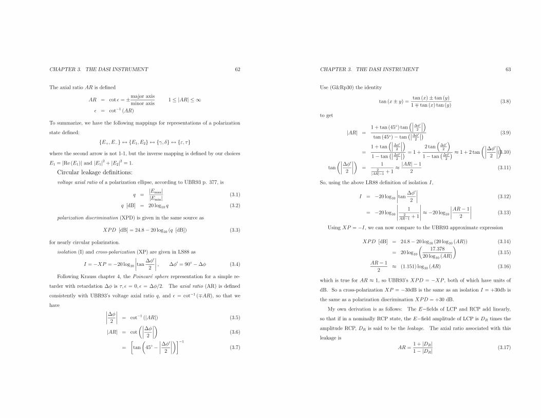
CHAPTER 3. THE DASI INSTRUMENT 62
The axial ratio AR is defined
AR = cot ε = ±major axis
minor axis1 ≤ |AR| ≤ ∞
ε = cot−1 (AR)
To summarize, we have the following mappings for representations of a polarization
state defined:
E+, E− ↔ E1, E2 ↔ γ, δ ↔ ε, τ
where the second arrow is not 1-1, but the inverse mapping is defined by our choices
E1 = |Re (E1)| and |E1|2 + |E2|2 = 1.
Circular leakage definitions:
voltage axial ratio of a polarization ellipse, according to UBR93 p. 377, is
q =|Emax||Emin|
(3.1)
q [dB] = 20 log10 q (3.2)
polarization discrimination (XPD) is given in the same source as
XPD [dB] = 24.8− 20 log10 (q [dB]) (3.3)
for nearly circular polarization.
isolation (I) and cross-polarization (XP) are given in LS88 as
I = −XP = −20 log10∣∣∣∣tan
∆φ′
2
∣∣∣∣ , ∆φ′ = 90 −∆φ (3.4)
Following Krauss chapter 4, the Poincare sphere representation for a simple re-
tarder with retardation ∆φ is τ, ε = 0, ε = ∆φ/2. The axial ratio (AR) is defined
consistently with UBR93’s voltage axial ratio q, and ε = cot−1 (∓AR), so that we
have∣∣∣∣∆φ
2
∣∣∣∣ = cot−1 (|AR|) (3.5)
|AR| = cot
(∣∣∣∣∆φ
2
∣∣∣∣)
(3.6)
=
[tan
(45 −
∣∣∣∣∆φ′
2
∣∣∣∣)]−1
(3.7)
CHAPTER 3. THE DASI INSTRUMENT 63
Use (G&Rp30) the identity
tan (x± y) = tan (x)± tan (y)
1∓ tan (x) tan (y)(3.8)
to get
|AR| =1 + tan (45) tan
(∣∣∣∆φ′
2
∣∣∣)
tan (45)− tan(∣∣∆φ′
2
∣∣) (3.9)
=1 + tan
(∣∣∣∆φ′
2
∣∣∣)
1− tan(∣∣∆φ′
2
∣∣) = 1 +2 tan
(∆φ′
2
)
1− tan(∆φ′
2
) ≈ 1 + 2 tan
(∣∣∣∣∆φ′
2
∣∣∣∣)(3.10)
tan
(∣∣∣∣∆φ′
2
∣∣∣∣)
=1
2|AR|−1
+ 1≈ |AR| − 1
2(3.11)
So, using the above LR88 definition of isolation I,
I = −20 log10∣∣∣∣tan
∆φ′
2
∣∣∣∣ (3.12)
= −20 log10
∣∣∣∣∣1
2AR−1
+ 1
∣∣∣∣∣ ≈ −20 log10∣∣∣∣AR− 1
2
∣∣∣∣ (3.13)
Using XP = −I, we can now compare to the UBR93 approximate expression
XPD [dB] = 24.8− 20 log10 (20 log10 (AR)) (3.14)
= 20 log10
(17.378
20 log10 (AR)
)(3.15)
AR− 1
2≈ (1.151) log10 (AR) (3.16)
which is true for AR ≈ 1, so UBR93’s XPD = −XP , both of which have units of
dB. So a cross-polarization XP = −30dB is the same as an isolation I = +30db is
the same as a polarization discrimination XPD = +30 dB.
My own derivation is as follows: The E−fields of LCP and RCP add linearly,
so that if in a nominally RCP state, the E−field amplitude of LCP is DR times the
amplitude RCP, DR is said to be the leakage. The axial ratio associated with this
leakage is
AR =1 + |DR|1− |DR|
(3.17)

CHAPTER 3. THE DASI INSTRUMENT 64
from which we can see immediately that |DR| = tan (∆φ′/2) ≈ ∆φ′/2.
Waveguide dispersion: From Pozar p. 173, the phase and group velocities
are
β =√k20 − k2c
vp =ω
β= c
koβ
vg = cβ
ko
Waveguide circular polarizers are one example of a class of devices some-
times known as “phase shifters,” “phase retarders,” or simply “retarders” in dual-
polarization waveguide. These devices are common components in microwave and
millimeter-wave antenna feed systems for communications, radar, and astronomical
applications and in other microwave and millimeter-wave systems. Circular polar-
izers can be used to couple linearly polarized components to either or both circular
polarizations. Other kinds of retarders can also be used to alter the overall phase or
angle of linear polarization of a signal. In applications where the orientation or the
retardation of these devices may be varied, these components are commonly used to
switch between linear, left-circular, and right-circular polarizations or to continuously
vary the phase or polarization state of a signal.
We will first describe a generic ideal retarder. The input and output ports of
a generic retarder are dual polarization waveguides which are usually of circular or
square cross section, although they may also be rectangular or elliptical, ridged or
corrugated, or generally of any other type which admits propagation of two orthogonal
electric field signal components. These two signal components can be labelled at
the input of the device as Vx,in and Vy,in and similarly at the output as Vx,out and
CHAPTER 3. THE DASI INSTRUMENT 65
Vy,out (see Fig 1a). The action of a generic retarder is to delay the propagation of
the signal component with a specific electric field orientation (labelled b) compared
to the propagation of the signal component with a linearly orthogonal electric field
(labelled a). The orientation of the electric fields of these two signal components,
which are orthogonal linear eigenmodes of the device, define the principle axes of the
retarder. If the x− and y−axes are chosen to align with these principle axes of the
retarder, and if the insertion loss of the retarder is negligible, then the action of this
ideal retarder can be described very simply:
Vx,out = e−iφaVx,in (3.18)
Vy,out = e−i(φa+∆φ)Vy,in. (3.19)
Both signal components receive a common phase shift φa, but the phase shift of the
Vy component φb = φa + ∆φ receives an additional phase retardation ∆φ compared
to the Vx component. Usually it is only this relative retardation ∆φ that is relevant
in applications.
If the retarder is rotated such that its principle axes are not aligned with the x−and y−axes, but are offset at an angle θ (as illustrated in Fig. 1a), then the action
of the ideal retarder can be described by the matrix equation
Vx,out
Vy,out
=
cos θ sin θ
− sin θ cos θ
e−iφa 0
0 e−i(φa+∆φ)
cos θ − sin θ
sin θ cos θ
Vx,in
Vy,in
(3.20)
If, as is usual, we neglect the overall phase φa, then matrix that represents the action
of the retarder depends only on the retardation ∆φ and the orientation θ.
An ideal quarter-wave retarder has retardation ∆φ = 90. An ideal half-wave
retarder has ∆φ = 180. Both are commonly used in applications at various ori-
entations θ. For example, an ideal circular polarizer is an application that can be

CHAPTER 3. THE DASI INSTRUMENT 66
realized by a quarter-wave retarder ∆φ = 90 set at orientation θ = 45, so that Vx,out
Vy,out
=
1√2
1 −i−i 1
Vx,in
Vy,in
. (3.21)
If at the input we excite only Vx,in (with Vy,in = 0), corresponding to a pure linearly
polarized input signal, then at the output Vx,out and Vy,out will have equal amplitude
but with a −90 relative phase shift, corresponding to pure right-handed circular
polarization. If the orientation of the retarder is changed to −45, then the opposite
(left-handed) circular polarization is produced, and if the orientation is 0 then linear
polarization is transmitted.
Another common application is a polarization rotator, which can be realized as a
half-wave retarder ∆φ = 180 with a variable orientation θ. For this device Vx,out
Vy,out
=
cos 2θ − sin 2θ
− sin 2θ − cos 2θ
Vx,in
Vy,in
. (3.22)
If again at the input we excite only Vx,in (with Vy,in = 0), corresponding to a pure
linearly polarized signal, then at the output we will still have a linearly polarized
signal, but with its E−field orientation rotated by an angle −2θ. It is well-known
that an application which combines a quarter-wave retarder at a variable orienta-
tion θ1 followed by a half-wave retarder at a variable orientation θ2 may be used
to couple an input signal of a given polarization state (e.g. pure linear Vx) to any
desired output polarization state, with arbitrary ellipticity and polarization orienta-
tion. Retarders may also be combined in other well-known combinations to realize
applications including fixed and continuously variable phase-shifters.
3.6 Existing Waveguide Polarizer Designs:
Existing actual waveguide retarder designs work by introducing structures or changes
in cross-section that are aligned with the principle axes of the retarder, so as to
CHAPTER 3. THE DASI INSTRUMENT 67
cause the electrical properties of the waveguide about these axes to differ. As a
result, signals with electrical fields oriented along either of these axes will propagate
at different speeds, producing a total relative phase shift ∆φ which may be tuned by
controlling the overall physical length of the retarder or the degree of difference in the
electrical properties that determine the two propagation speeds. It is thus relatively
easy to arrange a retarder to have a desired retardation ∆φ0 at some particular
frequency ν0. If the two propagation speeds were independent of the frequency of
the signals, then for a fixed overall length the retardation would be proportional to
frequency
∆φ (ν) ∝ ν (3.23)
resulting in relative retardation greater than ∆φ0 at frequencies higher than ν0, and
a retardation less than ∆φ0 at frequencies lower than ν0. In waveguide, however, the
propagation speed and corresponding total phase delay φa (ν) for a mode typically
depends not only on frequency but also on the cross-sectional geometry and on any
other structures whose electrical properties affect the propagation of that particu-
lar mode. The designer’s degree of control over the functional dependence φa (ν)
generally increases with increasing complexity of the cross-sectional geometry and/or
the structures that affect the propagation of that mode. The exact functional form
of ∆φ (ν) will depend on the details of that cross-sectional geometry and/or those
structures. By exploiting this, the designer of a waveguide retarder may arrange
for ∆φ (ν) = φb (ν)− φa (ν) to be “flatter” than the simple linear dependence of the
above equation would imply.
The usable bandwidth of a waveguide retarder, or of any device (like a circular
polarizer) that is based on retarders, will be limited to the range of frequencies over
which retardation error is less than some a specified tolerance
|∆φ (ν)−∆φ0| < δφtol. (3.24)
To achieve high-bandwidth, is thus desirable to choose a cross-sectional geometry

CHAPTER 3. THE DASI INSTRUMENT 68
and/or structures within the waveguide which not only introduce the desired relative
phase shift, but which also flatten ∆φ (ν) as much as possible over the desired band
of operation.
Some examples of conventional design strategies are illustrated in UBR93, for the
case of quarter-wave retarders intended for use as circular polarizers. Some of the sim-
plest designs (see figure 3.8.35) change only the relative cross-sectional height along
the principle axes, affecting only the relative cutoff frequencies of the two eigenmodes;
the resulting curves ∆φ (ν) are not very flat and increase monotonically across the
band. More sophisticated designs in common use may employ corrugations, ridges,
or dielectric slabs to effectively alter more than one parameter of the propagation
equations, so that a minimum may be achieved in ∆φ (ν) at which it is first-order
invariant in frequency:∂
∂ν∆φ (ν) = 0. (3.25)
For examples see UBR93 fig.3.8.40a, V00 fig. 7, and LS88 fig. 1b. This minimum may
be located exactly at a frequency ν0 for which ∆φ (ν0) = ∆φ0, maximizing flatness
at that frequency, or at a nearby frequency so that ∆φ (ν) = ∆φ0 has solutions at
two different frequencies, which is usually preferable for maximum usable bandwidth.
Still more sophisticated designs have been proposed (see LS88) which use these same
techniques, with increased complexity, to acquire another degree of control which can
achieve a second-order invariance in ∆φ (ν),
∂2
∂ν2∆φ (ν) = 0 (3.26)
or alternately permit a form of ∆φ (ν) for which ∆φ (ν) = ∆φ0 has solutions at three
frequencies (see LS88 fig. 2b).
Practical retarder designs must not only control the value of ∆φ0 and the flatness
of the curve ∆φ (ν). They must also have transition sections that are matched to
produce suitably low return loss. They must have suitably low ohmic and dielectric
losses in the waveguide walls and control structures. They must avoid excitation
CHAPTER 3. THE DASI INSTRUMENT 69
of unwanted higher-order modes. Often they must meet additional constraints of
manufacturing cost and repeatability. All of these tend to limit the complexity of
structures in practical conventional retarder designs.
The performance claimed by LS88 appears to be near the current practical limit
of this approach. They effectively achieve a second-order invariance in ∆φ (ν), with
∆φ = 90 ± 0.7 over a 28% bandwidth. When a quarter-wave retarder is used
as a circular polarizer, a phase error δφ ≤ 0.7 corresponds to a very low axial
ratio AR ≤ 0.1dB, where the axial ratio is a common measure of purity of circular
polarization. Other more commonly used designs, which achieve first-order invariance
in ∆φ (ν), and have been optimized for less precise applications, have been reported
with δφ ≤ 2.5 (AR ≤ 0.37dB) over bandwidths up to 40% (UBR93) and with
δφ ≤ 10 (AR ≤ 1.4dB) over bandwidths up to 61% (V00).
A common feature of all of these conventional retarder (and polarizer) designs
is that their cross sections are symmetrical about their principle axes. These axes
do not change throughout the length of a conventional retarder. They are well-
defined by the planes of mechanical symmetry of any such retarder, and allow us to
unambiguously define the orientation θ of the retarder. While, as described above,
in certain applications several retarders may be combined in sequence, set at different
orientations, in order to achieve a particular polarization coupling or variable phase
retardation at the central design frequency ν0, existing designs have not exploited any
such combinations to create a compound polarizer or retarder that achieves broad
bandwidth by cancelling the effects of frequency variation of ∆φ (ν). Rather, as we
have seen, existing designs have attempted to achieve broad bandwidth by suppressing
this variation of ∆φ (ν) by controlling the frequency-dependent propagation of the
orthogonal linear eigenmodes within individual retarders.

CHAPTER 3. THE DASI INSTRUMENT 70
3.7 The Multiple Element Approach
According to the invention, two or more individual retarders are coupled in specific
combinations, which are identified below, to cancel the frequency variation of the
performance of the compound device to any desired order of accuracy. Each element
of the compound polarizer or retarder is itself a conventional retarder, and may be
constructed according to any of the conventional retarder designs in common use.
Generally, the more elements in the compound design, the higher the order at which
the frequency variation of the performance can be cancelled, or alternatively the
greater the bandwidth over which a given precision specification can be met.
Because the compound device is composed of several conventional retarders, its
return loss and internal losses can be kept low by choosing conventional retarder de-
signs for the individual elements with suitably good performance. According to the
invention, these retarder elements must be coupled at certain specified orientation an-
gles, so that it may be most convenient to choose a circularly symmetric cross-section
at these transitions. The return loss and internal losses of the compound device will
depend on the losses and reflections of the individual elements and transition sec-
tions, and may be calculated for any specific choice of components using conventional
techniques known to those skilled in the art.
If the individual waveguide retarder elements are designed, as is usual, so that the
frequency variation of ∆φ (ν) for each is also suppressed, then the cancellation of the
frequency variation in the performance by the compound device is further enhanced.
For example, Fig. 2 illustrates the performance of a typical conventional quarter-wave
retarder used as a circular polarizer (labelled “1-element”). This typical retarder
has a single minimum in ∆φ (ν) (at which ∆φ is first-order invariant in frequency),
allowing it to achieve a precision of AR ≤ 0.35dB over 35% bandwidth. Using this
type of retarder in a compound two-element circular polarizer design, it is possible
CHAPTER 3. THE DASI INSTRUMENT 71
to achieve performance (as measured by AR) that is frequency invariant up to third-
order, or alternatively to have high precision over a much broader bandwidth, as is
illustrated. Increasing the number of elements to more than two improves the flatness
further, and with a small number of elements it is possible to achieve extremely high
precision over the entire usable bandwidth of the waveguide.
The situation for compound quarter-wave, half-wave, and other retarders is sim-
ilar. These devices have different performance measures than a circular polarizer,
but in all cases the use of additional elements allows a greater degree of frequency
invariance. A general procedure for identifying the specific combinations of retarder
elements and orientations that yield the highest order of frequency invariance for a
given kind of compound device (e.g. a three-element half-wave retarder) is described
below. The most useful combinations for compound circular polarizers, quarter-wave,
and half-wave retarders using up to four elements are specifically described.
The two-element circular polarizer design has been constructed, tested, and is
currently in use by the inventors with the DASI telescope. DASI uses these polarizers
to switch the response of each of its 13 antennas between left-circular and right-
circular, in order to make high-precision polarization measurements of the cosmic
microwave background between 26 and 36 GHz. The unprecedented broadband
performance of these polarizers has been confirmed by measurements, which show it
to be consistent with theoretical predictions.
3.7.1 formalism
In this section, we will first give a mathematical description of the action of a com-
pound device formed from multiple retarders. Next, we describe how the frequency
variation of the parameters which describe that action can be cancelled to a given
order by use of multiple retarders. We then identify the two parameters relevant

CHAPTER 3. THE DASI INSTRUMENT 72
for circular polarizers, and specify designs for two-, three-, and four-element com-
pound circular polarizers which cancel the frequency variation of these parameters to
progressively higher orders. We then do the same for compound quarter-wave and
half-wave retarders. Finally, we describe the construction of the two-element circular
polarizer and measurements of its performance.
If we define the matrix S
S (∆φ, θ) ≡
cos θ sin θ
− sin θ cos θ
e+i∆φ/2 0
0 e−i∆φ/2
cos θ − sin θ
sin θ cos θ
, (3.27)
as representing an ideal retarder element with retardation ∆φ set at orientation angle
θ (where the overall phase has been removed), the equation for the action of this
retarder, Eq. 3.20, becomes
Vx,out
Vy,out
= S (∆φ, θ)
Vx,in
Vy,in
. (3.28)
It is clear that if a second retarder S ′ = S (∆φ′, θ′) is coupled to the first such that the
signal Vx,out of the first is coupled to V ′x,in of the second, and likewise Vy,out = V ′
y,in,
then the action of the compound device will be given by the product of the two
matrices V ′
x,out
V ′y,out
= S (∆φ′, θ′)S (∆φ, θ)
Vx,in
Vy,in
. (3.29)
In general, the action of a compound retarder composed of n retarder elements (as
illustrated in Fig. 1b) can be written
Vx,out
Vy,out
= S (∆φn, θn) · · · S (∆φ2, θ2)S (∆φ1, θ1)
Vx,in
Vy,in
. (3.30)
By multiplying these matrices, the action of a compound retarder of n elements can
CHAPTER 3. THE DASI INSTRUMENT 73
be expressed as a single 2× 2 complex matrix Scompound
Scompound = S (∆φn, θn) · · · S (∆φ2, θ2)S (∆φ1, θ1) (3.31)
=
S31 S32
S41 S42
. (3.32)
The labelling that we use for the complex elements S31, etc., of this matrix reflects that
they are also actually elements of the 4× 4 scattering matrix, as it is conventionally
defined in microwave engineering literature, for the compound retarder considered as
a 4-port device with ports [Vx,in, Vy,in, Vx,out, Vy,out]. It is also possible to derive the
values of these elements by combining the full 4 × 4 scattering matrices of each of
the individual retarder elements, and in this way reflections and internal losses can
be accounted for exactly. If these are small, so that as above the retarders can be
regarded as ideal, then the matrix Scompound will be unitary. Because we have allowed
an overall phase to be removed, the determinant of this matrix det (Scompound) = 1.
It follows that the matrix can be written
Scompound =
S31 S32
− (S32)∗ (S31)
∗
with |S31|2 + |S32|2 = 1. (3.33)
It is evident that there are only 3 independent parameters that determine the matrix
Scompound, and thus define the action of the device. For example, we can choose these
parameters to be the phase of S31, α = arg (S31), the phase of S32, β = arg (S32), and
the ratio of their amplitudes, r = |S31| / |S32|. Other choices are possible. A given
application (e.g. circular polarizer or half-wave retarder) will dictate the required
values of some or all of these 3 parameters.
Any frequency variation of these parameters will be due to the frequency varia-
tion of the retardations ∆φi (ν) of each of the individual elements, i = 1...n, which
comprise the compound device. Using α as an example:
α = α (∆φ1 (ν) ,∆φ2 (ν) , ..,∆φn (ν) , θ1, θ2, ..., θn) (3.34)

CHAPTER 3. THE DASI INSTRUMENT 74
If each retarder element is chosen to be of a similar construction, although scaled in
length to produce the specified retardation at a central frequency ∆φ0i ≡ ∆φi (ν0),
we expect the fractional variation with frequency δ (ν) to be the same for all retarders
∆φi (ν) = [1 + δ (ν)]∆φ0i. (3.35)
We can use this to greatly simplify the frequency dependence in our expression for α
α = α (δ (ν) ,∆φ01,∆φ02, ..,∆φ0n, θ1, θ2, ..., θn) . (3.36)
For a given application which requires the parameter α to take the value α0, our task
will be to find a set of values for the 2n parameters (∆φ01,∆φ02, ..,∆φ0n, θ1, θ2, ..., θn)
such that at the center frequency, α = α0 and also one or more of the higher derivatives
δα/∂δ, ∂2α/∂δ2, etc., vanish. If the application requires other parameters (e.g., β
and r) to take specific values, we can write a set of 2n equations
2n equations
α0 = α(δ (ν0) ,
2n variables︷ ︸︸ ︷∆φ01,∆φ02, ..,∆φ0n, θ1, θ2, ..., θn)
0 = α′ (δ (ν0) ,∆φ01,∆φ02, ..,∆φ0n, θ1, θ2, ..., θn)
0 = α′′ (δ (ν0) ,∆φ01,∆φ02, ..,∆φ0n, θ1, θ2, ..., θn)
.. ...
β0 = β (δ (ν0) ,∆φ01,∆φ02, ..,∆φ0n, θ1, θ2, ..., θn)
0 = β′ (δ (ν0) ,∆φ01,∆φ02, ..,∆φ0n, θ1, θ2, ..., θn)
.. ...
r0 = r (δ (ν0) ,∆φ01,∆φ02, ..,∆φ0n, θ1, θ2, ..., θn)
0 = r′ (δ (ν0) ,∆φ01,∆φ02, ..,∆φ0n, θ1, θ2, ..., θn)
.. ...
(3.37)
where a prime denotes a partial derivative with respect to δ. These can be solved
for the 2n parameters (∆φ01,∆φ02, ..,∆φ0n, θ1, θ2, ..., θn) which cause α, β, r to take
their required values, and also to be invariant to variations in δ each to some specified
order. The equations above tend to be too cumbersome to manipulate analytically,
CHAPTER 3. THE DASI INSTRUMENT 75
but may be easily evaluated numerically by calculating
Scompound (δ,∆φ01,∆φ02, ..,∆φ0n, θ1, θ2, ..., θn) (3.38)
using the matrix equations
given above. Solutions for (∆φ01,∆φ02, ..,∆φ0n, θ1, θ2, ..., θn) can readily be found
using numerical grid search algorithms.
Note that in finding these solutions, no reference is made to the form of δ (ν). If
the retarder elements are designed so that at the central frequency v0 their retarda-
tions are first-order frequency invariant, so that
∂δ (ν0)
∂ν= 0, (3.39)
then if we expand δ (ν) about ν0, the leading order variation will be quadratic, δ ∝(ν − ν0)2. Similarly, if a solution for parameters of a compound device is found that
satisfies the equation a′ = 0, but the second derivative of α is unconstrained, then
the leading order variation of α will be quadratic in δ, or quartic in frequency
α− α0 ∝ δ2 ∝ (ν − ν0)4 . (3.40)
Thus, by combining first-order frequency-invariant retarders in a compound design
which cancels α′ = 0 to first order, we find that α is frequency-invariant to third
order. If the compound design cancels α′′ = 0 to second order, the result is that α
is frequency-invariant to fifth order! We call such solutions maximally flat, because
they achieve the highest possible precision near a central frequency. Alternatively,
several different frequencies can be substituted for the central frequency ν0 in Eqs.
3.37 and 3.39, resulting in α (ν) = α0 at up to four different frequencies for the α′ = 0
case, and up to six frequencies for the α′′ = 0 case. This latter approach we call
bandwidth optimized, because it generally allows one to achieve a given performance
specification for |α− α0| over the widest possible bandwidth. Typically it leads to a
solution for parameters (∆φ01,∆φ02, ..,∆φ0n, θ1, θ2, ..., θn) which differs very slightly
from the maximally flat solution.

CHAPTER 3. THE DASI INSTRUMENT 76
If the single retarder elements differ in construction or cross-section such that the
fractional variation δ of each element is not the same, the same approach can still
yield solutions if the values of the parameters and their derivatives with respect to ν
rather than δ are evaluated and constrained. The solutions in this case will depend
on the details of the differences in the fractional variation of each element.
NOTE: This is a way, e.g., to account for impact on the parameters of realistic
differences between the retarders due to difficulty in getting deltas to match exactly,
as well as the small effects of absorption and return loss. If those differences are
small, the solutions will again differ only slightly from the maximally flat solutions,
and optimization algorithms can take these as a starting point.
NOTE: If differences are large, it becomes possible to find other kinds of solutions,
e.g. “multi-segment” retarder solutions.
3.7.2 basic solutions
The action of a right-handed circular polarizer is to couple a signal linearly polarized
signal incident at Vx,in to Vx,out and Vy,out with equal amplitudes but with a −90
relative phase shift. In terms of the parameters defined above, this implies r = 1
and (α− β) = π/2. By the unitarity of the matrix Scompound, Vy,in will be coupled to
left-handed circular polarization. Only two parameters need to be constrained. The
unconstrained parameter represents a relative phase shift between the right- and left-
circular signals due to Vx,in and Vy,in, and is unimportant for applications which do
not use linear combinations of those signals. The leakage of a right-handed circular
polarizer, DR, may be defined as the complex amplitude of the left-handed circular
response,
DR =1√2(S31 − iS41) . (3.41)
CHAPTER 3. THE DASI INSTRUMENT 77
The voltage axial ratio may be defined in terms of the leakage,
V AR =
√1− |DR|2 + |DR|
√1− |DR|2 − |DR|
(3.42)
with the axial ratio AR in dB given by
AR = 20 log10 (V AR) . (3.43)
Thus, the leakage is a convenient to work with, and we choose to constrain its real
and imaginary parts (and some of their derivatives) to be zero
x = Re (DR) , x0 = 0 (3.44)
y = Im (DR) , y0 = 0 (3.45)
when solving the system Eq. 3.37. This is equivalent to constraining parameters r
and (α− β). Because we have two parameters, for an n-element compound circular
polarizer, we use the 2n equations to constrain the parameter values and their first
n−1 derivatives. For n = 1...4, our numerical search identifies the following preferred
maximally-flat designs:
circular polarizer designs:
n constrained: ∆φ01 θ1 ∆φ02 θ2 ∆φ03 θ3 ∆φ04 θ4
1 x, y 90 45
2 x, y, x′, y′ 180 15 90 75
3 x, y, x′, y′, x′′, y′′ 180 6.05 180 34.68 90 102.27
4 x, y, x′, y′, x′′, y′′, x′′′, y′′′ 180 23.13 180 151.80 180 53.53 90 74.71
The performance of these designs, using typical retarder elements, is illustrated
in Fig. 2. The 1-element design, listed for comparison, is the conventional circular
polarizer formed from a single quarter-wave retarder at 45. For each design, if the
orientation of every element is reflected θi → π/2 − θi, equivalent designs that work

CHAPTER 3. THE DASI INSTRUMENT 78
equally well are obtained. Other, distinct designs may also be found for 2, 3, and
4 elements, but they are less desirable, having greater total retardations Σi∆φi and
therefore longer total physical length and internal losses.
For applications which may use arbitrary linear combinations of the signals due
to Vx,in and Vy,in, generally three parameters of the action must be constrained. For
example, half-wave retarders are often used as linear polarization rotators, with the
overall orientation angle of the device continuously variable, so that the input signal
may be any combination of Vx,in and Vy,in. Similarly, quarter-wave retarders can be
used to switch between circular and linear response; for either of these devices, if
the third parameter is left unconstrained (as for the circular polarizers above), the
orientation angle of the linear output will be unconstrained, and will generally vary
with frequency.
For these designs, three parameters we choose to constrain are
x = Re (S41) , x0 = 0 (3.46)
y = Im (S41) , y0 = 0 (3.47)
z = arg (S31)− arg (S42) = ∆φeffective. (3.48)
For quarter-wave retarders, we constrain z0 = π/2. For half-wave retarders, we
constrain z0 = π. Because we have 3 parameters, for an n-element compound
retarder, we must choose which of higher derivatives of these parameters to constrain
with our 2n equations. For various choices and for n = 1...4, our numerical search
identifies the following preferred maximally-flat quarter-wave designs:
quarter-wave designs:
n constrained: ∆φ01 θ1 ∆φ02 θ2 ∆φ03 θ3 ∆φ04 θ4
1 x, z, (y = 0 also) 90 0
2 x, y, z, z′ 90 0 360 52.24
3 x, y, z, x′, y′, z′ 115.18 30.98 180 140.28 115.18 30.98
4 x, y, z, x′, y′, z′, x′′, z′′ 250.48 17.36 180 115.84 180 166.57 140.77 60.95
CHAPTER 3. THE DASI INSTRUMENT 79
and the following preferred maximally-flat half-wave designs:
half-wave designs:
n constrained: ∆φ01 θ1 ∆φ02 θ2 ∆φ03 θ3 ∆φ04 θ4
1 x, z, (y = 0 also) 180 0
2 x, y, z, z′ 180 90 360 30
3 x, y, z, x′, y′, z′ 180 60 180 120 180 60
4 x, y, z, x′, y′, z′, x′′, y′′ 180 90 180 37.78 360 23.28 180 127.78
As before with the circular polarizer designs, we have listed the 1-element designs,
which are the corresponding conventional quarter- and half-wave devices, strictly for
comparison. Also as before, for each design, if the orientation of every element is
reflected θi → π/2−θi, and for half-wave designs also θi → π/2+θi, equivalent designs
that work equally well are obtained. Other, distinct designs may also be found for
2, 3, and 4 elements, but they are less desirable, having greater total retardations
Σi∆φi and therefore longer total physical length and internal losses.
3.7.3 bandwidth optimization
3.7.4 additional applications
3.8 Design and Construction of the DASI Polariz-
ers
The two-element circular polarizer design has been constructed, tested, and is cur-
rently in use by the inventors with the DASI telescope. DASI uses these polarizers to
switch the response of each of its 13 antennas between left-circular and right-circular,
in order to make high-precision polarization measurements of the cosmic microwave
background between 26 and 36 GHz.

CHAPTER 3. THE DASI INSTRUMENT 80
The construction of this device is illustrated in Fig. 3a, b, c, d, and e. The
compound polarizer is composed of a circular waveguide section, illustrated in Fig
3a., which contains two retarder elements in the form of shaped dielectric slabs,
illustrated in Fig 3b and c.
The circular waveguide section is machined from brass, and is gold-plated to en-
hance conductivity of the inner walls. Each end of the waveguide section incorporates
an outer step (OD 0.5490 in.) that forms a race for a ball-bearing, allowing the sec-
tion to rotate freely. A gear is fixed to the outer diameter of the waveguide section
to allow it to be driven to any desired orientation. Each end of the waveguide section
also incorporates an inner step (diameter 0.4280 in.) which forms a choke groove
at the bearing gap, preventing leakage of microwave power through the gap. The
inner walls of the waveguide section are broached with two pairs of precise grooves,
a long pair and a short pair, set at 60 from each other. These hold and define the
angular orientation of the dielectric slab retarder elements. The first retarder ele-
ment, ∆φ01 = 180, slides into the long grooves, and the second retarder element,
∆φ02 = 90, slides into the short grooves from the opposite end. When the gear is
driven to rotate the waveguide section so that the long grooves and the first element
are at θ1 = 15 from the input orientation, then the second element is at θ2 = 75
and the compound device couples to right-handed circular polarization. When the
gear rotates the waveguide section so that the first element is at θ1 = −75 , then
the second element is at θ2 = −15 and the device couples to left-handed circular
polarization.
The two retarder elements are dielectric slabs made from polystyrene, which was
chosen for its low dielectric loss, dimensional stability, and ease of machinability.
Other dielectric materials, for example teflon, polyethylene, or fused quartz, may also
be used. In order to improve match and minimize reflections at the ends of the slabs,
the profiles of those ends taper to points, as illustrated in Fig. 3b and 3c. The
particular choice of the dual-pointed profile was optimized to eliminate excitation of
CHAPTER 3. THE DASI INSTRUMENT 81
the unwanted TM11 mode. The edges of the slabs are keyed with a ridges, which
fit into the grooves of the waveguide section, as illustrated in Fig 3d. The slabs are
press-fit, and are secured in place with a small dot of epoxy. The entire assembly of
the compound polarizer, comprising the waveguide section and the two polystyrene
retarder elements, is illustrated in Fig. 3e.
3.9 Tuning, Testing, and Installation
The retardation curves ∆φ1 (ν) and ∆φ2 (ν) were measured for these two retarders
using a Hewlett-Packard HP8722D vector network analyzer. The relative phase shift
between signals with electric fields oriented parallel to and perpendicular to the slabs
was measured by differencing the propagation phases (∠S21) with the slab in each of
these positions. The resulting curves for the first and second retarder elements are
shown in Figs. 4a and 4b, respectively. It can be seen that the fractional variation
with frequency δ (ν) is well-matched for these two retarders. The variation δ (ν) van-
ishes to first-order at ν0 ≈ 26GHz. Unfortunately, this is at the edge, not the center,
of the desired operating band 26-36GHz. A choice of waveguide diameter smaller
than 0.315 in. would have shifted this ν0 up toward our band center, but manufac-
turing time constraints for this prototype prevented that optimization. Nonetheless,
even though the variation δ (ν) is not optimally flattened for these retarder elements,
the cancellation of this variation due to the compound design leads to unprecedented
broadband precision for this polarizer. Return loss was also measured in both orien-
tations for these dielectric slab retarder elements, and found to nowhere exceed −20dB.
The performance of the complete assembled compound polarizer was measured
with the polarizer installed in a DASI receiver, using a laboratory setup illustrated
in Fig. 4d. A transmitter which produces a strong, broadband, linearly polarized
signal is rotated continuously about the axis of its horn at 2 Hz (120 RPM). The

CHAPTER 3. THE DASI INSTRUMENT 82
horn of the fixed receiver couples directly to this rotating linear signal in an anechoic
box made of microwave absorbing material, to eliminate multiple reflections. If the
receiver is fitted with a perfect circular polarizer, the power output will be steady.
However, if the response is elliptical, the power output will be modulated as the
orientation of the linear signal changes, reaching a maximum each time the rotating
source is aligned with the major axis of the polarization ellipse. The LO, mixer, and
filter bank allow selection of each of ten sub-bands within 26-36 GHz, to measure
performance across the entire frequency range of the polarizer. The Hewlett-Packard
HP437B power meter measures the microwave power output of the receiver in each
sub-band and outputs that power level as a 0-10V signal. The Stanford Research
Systems SR840 lock-in amplifier measures the synchronous modulation of this signal,
allowing the axial ratio and orientation of the polarizer’s ellipse to be determined at
each frequency.
Fig. 4c illustrates the results of this laboratory measurement of the axial ratio
of the DASI compound polarizer in both right-circular and left-circular orientations.
For comparison, a conventional single-element polarizer built using the same type of
retarder is shown. In both cases, the data closely match the theoretical predictions.
With the polarizers in receivers installed on the DASI telescope, separate calibration
procedures using astronomical sources confirm these measurements. In laboratory
testing and in use, the compound 2-element polarizer has been demonstrated to give
unprecedented broadband performance.
3.10 Polarizer Switching
Since the DASI correlator was originally designed to accommodate only a single Stokes
state per IF, observation in all four states is achieved via time-multiplexing. The
polarizer for each receiver is switched between L and R on a Walsh sequence which
spends an equal amount of time in each state, i.e.,∑
i fi = 0 if we represent the two
CHAPTER 3. THE DASI INSTRUMENT 83
states as f ∈ ±1. The product of two Walsh functions is another Walsh function,
whence∑
i,n6=m fni f
mi = 0, and the baseline therefore spends an equal amount of time
in the co-polar (RR, LL) and cross-polar (LR, RL) states. In fact, it can be shown
that with this sequencing of the polarizers, over the course of a full Walsh cycle each
baseline of the interferometer spends an equal amount of time in each of the four
Stokes states, although different baselines will sample different Stokes states at any
given time. For the observations presented here, a Walsh function of period 16 with
a time step of 200 seconds was used, so that over the course of an hour, every Stokes
state is sampled by every baseline for approximately 13 minutes.
3.11 New Design Directions
Dual polarization desirable; with new designs, OMTs become limiting factor.

CHAPTER 3. THE DASI INSTRUMENT 84
Ka36title: Ka36_b−cold
tested: 11/05/99
temperature: 10.05K
LEDs: ON
test port: B
devices installed:stage 1 2 3 4
gate (microns) 100 100 100 100
GM@LN 540 527 490 464
device 49512174951216 51511825151183
bond distance 24.6 24.2 19.2 19.9
bond height 3.0 3.0 2.5 3.0
biases:stage 1 2 3 4
Vd 1.00 1.00 1.00 1.00
Id (mA) 2.00 3.00 3.00 3.00
Vg −0.337 −0.345 −0.146 −0.114
Ig (µA) 0.0 0.0 0.0 0.0
PO Id (mA) 0.05 0.05 0.05 0.05
PO Vg −0.500 −0.500 −0.500 −0.500
22 23 24 25 26 27 28 29 30 31 32 33 34 35 36 37 38 39 4010
15
20
25
30
35
40
45
50
55
60
65
70
GHz
nois
e te
mpe
ratu
re, K
Noise files:Ka36_1Ka36_2Ka36_3Ka36_4
alt files:
Ka36_5
−16
−12
−8
−4
0
4
8
12
16
20
24
28
32
36
40
S11
S12
S21
S22
dB
Gain file:Ka36_b
Figure 3.6 Response in the uv plane of an RL-LR combination baseline. The upper panel shows
the response in the Q plane, the lower panels show the same response after transforming to E and
B.
CHAPTER 3. THE DASI INSTRUMENT 85
Figure 3.7 The cation of the two-element polarizer is illustrated on the Poincare sphere. Polariza-
tion ellipses to the right.
Figure 3.8 The cation of the two-element polarizer is illustrated on the Poincare sphere. Polariza-
tion ellipses to the right.

CHAPTER 3. THE DASI INSTRUMENT 86
25 30 35 40 45 500
0.01
0.02
0.03
0.04
0.05
0.06
ν, GHz
frac
tiona
l lea
kage
performance comparison of typical 1, 2, 3, and 4 element polarizers
1 element2 element3 element4 element
Figure 3.9 Comparison of the instrumental polarization for single and multi-element polarzers.
Shown are the theoretical minimum leakage for a single-element polarizer (dashed line) and for
multi-element polarizers of 2-elements (solid line), 3 elements (dot-dash line), and 4 elements
(dot-dot-dash line).
Figure 3.10 Drawing of the DASI broadband polarizers. Shown is the rotating barrel piece and the
two dielectric retarder elements which it houses. The brass barrel is driven by a gear (not shown)
mounted around its midline, and rotates on dry ball bearings which run in the square races at either
end, just outside of the step which forms a choke groove. The dual-pointed profile of the polystyrene
dielectric pieces minimized coupling to the unwanted TM11 mode. Waveguide diameter is 0.315”,
total length of the barrel is 2.016”.
CHAPTER 3. THE DASI INSTRUMENT 87
Figure 3.11 Drawing of the DASI broadband polarizers. Shown is the rotating barrel piece and the
two dielectric retarder elements which it houses. The brass barrel is driven by a gear (not shown)
mounted around its midline, and rotates on dry ball bearings which run in the square races at either
end, just outside of the step which forms a choke groove. The dual-pointed profile of the polystyrene
dielectric pieces minimized coupling to the unwanted TM11 mode. Waveguide diameter is 0.315”,
total length of the barrel is 2.016”.

CHAPTER 3. THE DASI INSTRUMENT 88
Figure 3.12 Configuration for laboratory tests of circular polarizer performance. A transmitter
which produces a broadband linearly polarized signal is rotated continuously at 2 Hz (120 RPM).
If the fixed receiver is fitted with a perfect circular polarizer, the power output will be steady. Any
elipticity of the polarizer will cause a modulation of the power output as the orientation of the linear
signal changes. The SR840 lock-in amplifier measures this synchronous modulation, allowing the
axial ratio and orientation of the ellipse to be determined. The LO, mixer, and filter bank allow the
power meter to select each of ten sub-bands within 26-36 GHz, to measure performance across that
frequency range.
CHAPTER 3. THE DASI INSTRUMENT 89
300 K 26-36 GHzpolarizer
26-36 GHz
2-12 GHz
38 GHz LO
2-3 3-4 4-5 5-6 6-7 7-8 8-9 9-10 10-11 11-12 GHz
filter bank
HP 3478Apower meter
SR 840lock-in amplifier
analog outputsignal intrigger
2 Hz
anechoic box
rotating transmitter
fixed receiver
RF power in
2 Hz
Figure 3.13 Configuration for laboratory tests of circular polarizer performance. A transmitter
which produces a broadband linearly polarized signal is rotated continuously at 2 Hz (120 RPM).
If the fixed receiver is fitted with a perfect circular polarizer, the power output will be steady. Any
elipticity of the polarizer will cause a modulation of the power output as the orientation of the linear
signal changes. The SR840 lock-in amplifier measures this synchronous modulation, allowing the
axial ratio and orientation of the ellipse to be determined. The LO, mixer, and filter bank allow the
power meter to select each of ten sub-bands within 26-36 GHz, to measure performance across that
frequency range.

CHAPTER 3. THE DASI INSTRUMENT 90
22 24 26 28 30 32 34 36 38 400
0.05
0.1
0.15
ν, GHz
leak
age
ampl
itude
Comparison of conventional vs. DASI 2−element polarizers
1 element (theory)1 element (measured)2 element (theory)2 element (measured)
Figure 3.14 Comparison of the instrumental polarization for single and multi-element polarzers.
Shown are the theoretical minimum leakage for a single-element polarizer (dashed line), and for a
2-element polarizer (solid line). Squares are benchtop measurements of a single-element polarizer.
Points are the astronomical measurements of the average on-axis instrumental polarization for the
13 DASI receivers configured with 2-element polarizers.
Figure 3.15 Drawing of a new all-metal W-band polarizer design. This design replaces the dielec-
tric elements of the DASI broadband polarizers with a combination of corrugations and indented
waveguide walls, but uses the same two-element circular polarizer combination of retarder lengths
and angles. Wageguide diameter is 0.122”, total length is 1.5”.
CHAPTER 3. THE DASI INSTRUMENT 91
70 80 90 100 110 120 130−50
−40
−30
−20
−10
0
retu
rn lo
ss, d
B
frequency, GHz
−0.04
−0.02
0
0.02
0.04
0.06
0.08
leak
age
realimaginarytotal
Figure 3.16 Modeled performance of the new W-band polarizer design. Ansoft HFSS software was
used to simulate operation over the indicated range of frequencies.

Chapter 4
Calibration
In Paper IV, we detail the calibration of the polarized visibilities for an interferome-
ter. In order to produce the calibrated visibilities as defined in Equation 2.12 below, a
complex gain factor which depends on the Stokes state S must be applied to each raw
visibility. Although the cross-polar gain factors could easily be determined with obser-
vations of a bright polarized source, no suitable sources are available, and we therefore
derive the full calibration through observations of an unpolarized source. The gains
for a given pair of receivers m−n (a baseline) can be decomposed into antenna-based
factors, allowing us to construct the cross-polar gains from the antenna-based gain
factors derived from the co-polar visibilities. DASI’s calibration is based on daily
observations of the bright HII region RCW38, described at length in Paper I. We can
determine the individual baseline gains for all Stokes states with statistical uncertain-
ties < 2% for each daily observation. Systematic gain uncertainties for the complete
dataset are discussed in §6.3.During the course of the 2001 – 2002 CMB observations, considerable effort was
expended to characterize the polarization response of the instrument through observa-
tions of astronomical sources. In the preceding sections, we have described at length
observations of the unpolarized HII region RCW38, on which the bulk of DASI’s
calibration is based. Here we present polarimetric observations of a variety of other
sources which provide independent checks of those calibrations, and lend confidence
92
CHAPTER 4. CALIBRATION 93
that we understand the various aspects of the instrumental response to a level (pre-
cision better than 1%) beyond that required to measure polarization in the CMB.
4.1 Relative Gain and Phase Calibration
(OK, trying to use notation common to Erik’s notes (EL1/01), TMS §4.9 and §10.1,and NRAO §5.7.5 and §5.9)
Antenna-based gain solutions:
The baseline-based complex gain (NRAO eq. 5-14) for a single correlator channel
(i.e. 1 of 78 per band) is defined
Gij =VijS
(4.1)
where Vij is the uncalibrated complex visibility for that channel when observing
a point source at phase center of flux density S. Thus, Gij has units of (data
units)/(Jy). We can write
Gij = gig∗j gij (4.2)
breaking the gain into antenna-based gains gi and gj, and a residual baseline-based
gain gij. In NRAO §5.7.5 the discussion of solving for an antenna based gains gi is
based on the premise that the gij, which physically have to do with the correlator,
are all close to (within ˜1%) of unity. This will generally not be true for analog
correlators, and despite an approximate matching of correlator path lengths, we know
from the size of the real vs. imag correction factors we apply that it is not true for
DASI.
What happens to your solution if the gij − 1 are not small? I think it depends
on your algorithm. Generally, though, you have 78 (complex) equations in 78+13
unknowns, and so to find a unique solution you must place additional constraints.
For example, you can require that the mean of all 12 gij associated with a given
antenna be 1, for each of the 13 antennas. Whatever your algorithm for arriving at

CHAPTER 4. CALIBRATION 94
the gi, you can use the residual “closure terms” gij = Gij/gig∗j , which for DASI should
be significant, to correct your antenna-based gains back to the (more accurate, for
us!) baseline based gains of eq. 4.2.
Polarization baselines
Generalize the above to include the switchable polarization state, X = L or R,but still assuming a hypothetical point source at phase center of flux density S, now
also with linear polarization SQ and SU (also in Jy):
GLLij =
V LLij
S= gLi g
L∗j gij
GRRij =
V RRij
S= gRi g
R∗j gij
GRLij =
V RLij
[e−2iχ (SQ + iSU) + (DR1 +D∗L2)S]
= gRi gL∗j gij
GLRij =
V LRij
[e2iχ (SQ − iSU) + (DL1 +D∗R2)S]
= gLi gR∗j gij
GXX′
ij = gXi gX′∗j gij
We can and do get the GLLij and GRR
ij from observing a bright calibrated source (say,
RCW38) of known flux S. Our goal is to determine the GRLij and GLR
ij (at least to
a single overall phase ∆ψ) without requiring cross-polarized observations of a bright
polarized source of known SQ and SU (there are none suitable!).
If we could use our measurements of GLLij and GRR
ij to directly solve for antenna-
based gain solutions for the gLi and the gRi , and if we could calculate the closure
terms gij needed for baseline-based corrections, we would be done. For this to work,
though, the closure terms gij derived from the LL and from the RR antenna-based
solutions (which are naturally underconstrained) need to be identical; otherwise the
gLi and the gRi are not equivalent and cannot be combined together with these gij in
expressions for GRLij and GLR
ij
But perhaps rather than trying to force these antenna-based gain solutions algo-
rithms to do something they were not intended for, it may be better to take a different
CHAPTER 4. CALIBRATION 95
approach. Start with
GLLij = gLi g
L∗j gij
GRRij = gRi g
R∗j gij
and simply divide:
GLLij
GRRij
=gLi g
L∗j gij
gRi gR∗j gij(
GLL
GRR
)
ij
=
(gL
gR
)
i
(gL
gR
)∗
j
1
Now we have an equation of exactly the form that you want for doing antenna-based
solutions; the baseline-based factor should be identically unity to within measurement
error. We can solve for the antenna-based ratios(gL
gR
)iup to the overall phase ∆ψ
which is always arbitrary in such solutions. We can then test that the new “closure
ratios”(GLL
GRR
)ij/(gL
gR
)i
(gL
gR
)∗jare indeed nearly 1. If so, we can confidently calculate
GRLij = gRi g
L∗j gij =
gL∗jgR∗j
gRi gR∗j gij =
(e−i∆ψ
)(gLgR
)∗
j
GRRij
GLRij = gLi g
R∗j gij =
gLigRigRi g
R∗j gij =
(ei∆ψ
)(gLgR
)
i
GRRij
and only the single overall phase ∆ψ is undetermined.
In practice, each receiver introduces a unique phase offset and amplitude variation
to the electric field, so that the expression for the detected field must be modified by a
receiver-dependent complex gain, Em = gmEm, where gm depends on the polarization
state of the receiver. Furthermore, the correlator can introduce baseline-dependent
complex gains gmn, independent of polarization state, so that the measured visibilities
are given by:

CHAPTER 4. CALIBRATION 96
V RRmn = gRmg
Rn
∗gmnV
RRmn ≡ GRR
mnVRRmn
V LLmn = gLmg
Ln
∗gmnV
LLmn ≡ GLL
mnVLLmn
V RLmn = gRmg
Ln
∗gmnV
RLmn ≡ GRL
mnVRLmn
V LRmn = gLmg
Rn
∗gmnV
LRmn ≡ GLR
mnVLRmn . (4.3)
Since the co-polar visibilities V RRmn and V LL
mn are just proportional to Stokes SI±SV ,the gain factors GRR
mn and GLLmn can simply be derived on a per-baseline basis from
observations of a bright unpolarized point source, or more complicated source whose
intrinsic visibility structure is known (if we take the circular polarization SV to be
zero).
However, we require a source of known linear polarization to derive the complex
gains in the same manner for the cross-polar visibilities V RLmn and V LR
mn . These are
in general scarce at high frequencies, and furthermore few are well studied in the
southern hemisphere. The low gain of DASI’s 20-cm feed horns, moreover, makes
it impracticable to observe all but the brightest sources, in total intensity or other-
wise, and the brightest sources at 30 GHz are typically compact HII regions, whose
polarization fraction is expected to be negligible.
As can be seen from Equation 4.3, however, we can in principle derive the cross-
polar gains from co-polar observations of an unpolarized source, if we work in ratios
of complex gains:V LLmn
V RRmn
=
(gL
gR
)
m
(gL
gR
)∗
n
≡ rmr∗n (4.4)
in which the correlator gains gmn exactly cancel. For DASI, this yields an overcon-
strained set of 78 complex equations which can be solved for the 13 antenna-based
ratios rk = gLk /gRk .
The solution is not unique, and we must arbitrarily specify the phase ∆φ ≡ φR−φLof one of the ratios, typically setting it to zero. With the ratios rk in hand, the
CHAPTER 4. CALIBRATION 97
26 28 30 32 34 36
−25
−20
−15
−10
−5
ν (GHz)
∆φ (
°)
Figure 4.1 DASI absolute phase offsets. Shown are phase offsets determined from wire grid ob-
servations (triangles) and from the Moon (circles). Also shown are benchtop measurements of the
same polarizer (solid line, squares), with an arbitrary offset subtracted.
baseline complex gains for the cross-polarized channels can be recovered from the
co-polar solutions as:
r∗nGRRmn =
(gL
gR
)∗
n
gRmgRn
∗gmn = e−i∆φGRL
mn
rmGRRmn =
(gL
gR
)
m
gRmgRn
∗gmn = ei∆φGLR
mn (4.5)
that is, we can construct the cross-mode calibration factors from the antenna-based
solutions, but only up to the unknown phase difference between R and L for our
reference antenna. This overall phase offset, while leaving the amplitude of the cross-
polar visibilities unaffected, will mix power between SQ and SU , or between E and B,
in terms of the decomposition into the coordinate-independent scalar fields which has
become the standard in the CMB polarization literature (Kamionkowski et al. 1997b;
Zaldarriaga & Seljak 1997; Hu & White 1997). Removal of the offset is therefore
critical to obtaining a clean separation of CMB power into E- and B-modes.
In practice, we use the bright, compact, unpolarized HII region, RCW38, to de-
termine the co-polar and cross-polar calibration factors in this manner. The phase
offset can only be determined by observing a source whose plane of polarization is

CHAPTER 4. CALIBRATION 98
known, as described in the next section.
4.2 Absolute Crosspolar Phase Calibration
The procedure for deriving the baseline gains from antenna-based terms leaves the
cross-polar visibilities multiplied by an undetermined overall phase offset (indepen-
dent of baseline). This phase offset effectively mixes Q and U , and must be measured
to obtain a clean separation of CMB power into E- and B-modes. Calibration of
the phase offset requires a source whose polarization angle is known, and we create
one by observing RCW38 through polarizing wire grids attached to DASI’s thirteen
receivers. From the wire-grid observations, we can derive the phase offset in each
frequency band with an uncertainty of . 0.4.
As an independent check of this phase offset calibration, the Moon was observed at
several epochs during 2001–2002. Although the expected amplitude of the polarized
signal from the Moon is not well known at these frequencies, the polarization pattern
is expected to be radial to high accuracy, and this can be used to determine the cross-
polar phase offset independently of the wire grid observations. As shown in Paper
IV, these two determinations of the phase offset are in excellent agreement.
To determine the phase offset introduced by the complex gain correction described
above, we require a source whose polarization angle (though not amplitude) is known.
As discussed in §4.1, however, few suitably strong polarized sources are available, and
in practice we create a source of known polarization angle by observing an unpolarized
source through polarizing wire grids. At centimeter wavelengths, the required wire
spacing (. λ/3) poses no particular technical challenges, and grids can be simply
constructed out of conventional materials; thirteen wire grids were constructed out
of 34-gauge copper wire, wound with a spacing of 0.05′′. These grids attach directly
to the exterior of the corrugated shrouds and completely cover the aperture of the
DASI horns.
CHAPTER 4. CALIBRATION 99
The same source used for gain calibration of the visibilities, RCW38, was observed
with the wire grids attached in two orientations, one with wires parallel to the ground,
and the other with grids (but not receivers) rotated by 45 degrees with respect to the
first. It was confirmed that in the second orientation the apparent phase of the cross-
polar visibilities shifted by ±90 relative to the first, as indicated by Equation 2.12.
The measured absolute phase offsets ∆φ(ν) are shown in Figure 4.1. These offsets
show a trend in frequency which is a direct consequence of the achromatic polarizer
design discussed in §??. As Figure 4.1 shows, this trend is in excellent agreement
with expectations from benchtop measurements of the polarizers, where the expected
trend is shown with an arbitrary offset subtracted. These phase offsets were measured
in 2001 August and again in 2002 February and were found to agree within measure-
ment errors. As discussed below, we can restrict the intrinsic polarization fraction
of RCW38 to < 0.09% at our observing frequency; since the grids create a polarized
source with an effective polarization fraction of 100%, any intrinsic polarized flux
at this level will have a negligible effect on the measurements of the absolute phase
offsets.
Although suitably bright point sources of known polarization angle are not avail-
able, we can in principle derive the absolute phase offsets from observations of the
Moon, as discussed in §??. These results, also shown in Figure 4.1, are consistent with
the offsets measured with the wire grid polarizers, to within the ∼ 0.4 measurement
errors. As discussed in Paper V, errors in the absolute phase offset of this magnitude
have a negligible effect on the power spectral analysis.
At centimeter wavelengths, radiation from the Moon is dominated by thermal
emission from the regolith, typically from the first ∼ 10 – 20 cm of the Moon’s
surface. This radiation is intrinsically unpolarized, but scattering off the dielectric
discontinuity at the surface will induce polarization; the tangentially polarized com-
ponent is preferentially reflected, leading to a net radial polarization pattern across
the disk of the Moon. This polarization amplitude decreases to zero at the center

CHAPTER 4. CALIBRATION 100
and increases to a maximum at the limb (see Moffat (1972) for a comparable result
at 21 cm, and Mitchell & De Pater (1994) for a similar discussion and map of the
microwave polarization of Mercury).
Observations of the Moon were made with DASI during 2001 – 2002 at several
epochs, and at various phases of the Moon. All show excellent agreement with the
expected radial polarization pattern, and the consistency between epochs attests to
the stability of the absolute phase offset. In Figure 4.4 we present a polarized map
of the Moon made during 21 – 22 August 2001, when the Moon was nearly full.
These data have been corrected for instrumental leakages and the absolute phase
offset determined from wire grid observations, discussed in §4.2.Note that any residual phase offset in the cross-polar visibilities will introduce
a vorticity to the polarization vectors, from which we can derive an independent
measure of the cross-polar phase offsets. These measurements are shown in Figure 4.1,
and are in excellent agreement with the phase offsets determined from the wire grid
observations discussed in §4.2.NOTE: a single cross-polar phase offset was derived and applied to all epochs of
data. This is referenced to rx? and should be time stable. Observations are consistent
with this.
4.3 Absolute Gain Calibration
4.4 Leakage Correction
For ideal polarizers, the cross-polar visibilities are strictly proportional to linear com-
binations of the Stokes parameters Q and U . For realistic polarizers, however, imper-
fect rejection of the unwanted polarization state leads to additional terms in the cross-
polar visibilities proportional to the total intensity I. These leakage terms are the
sum of the complex leakage of the two antennas which form each baseline. During the
CHAPTER 4. CALIBRATION 101
−4−2024−4
−2
0
2
4
X offset (deg)
Y o
ffset
(de
g)
0 2 4 6 8
0
0.2
0.4
0.6
0.8
Radius from field center (deg)
Per
cent
Pol
ariz
atio
n Le
akag
e
Figure 4.2 DASI off-axis leakage measurements. (left) The measured direction of the instrumental
leakage for a ring of 2.5 offset pointings on RCW38. (right) The amplitude profile of the instrumental
polarization shown versus radius from field center. Moon data are shown as red, green and blue
circles corresponding to the frequency bands 26 – 29, 29 – 33, and 33 – 36 GHz respectively. RCW38
data for the full 26 – 36 GHz band are shown as black points. The green line is a spline interpolation
of the 29 – 33 GHz Moon data, and the red and blue dashed lines are the interpolation scaled to
27.5 and 34.5 GHz respectively. See text for further discussion.
2000–2001 austral summer, DASI’s thirteen receivers were retrofit with multi-element
broadband circular polarizers designed to reject the unwanted polarization state to
high precision across DASI’s 26 – 36 GHz frequency band. Prior to installation on
the telescope, the polarizers were tuned to minimize these leakages.
As discussed in §??, the receivers are mounted on a rigid faceplate which can be
driven to simulate parallactic angle rotation. From Equation ??, it can be seen that
the leakages are irrotational, while any contribution to the visibilities from intrinsic
source polarization will have a phase modulated by the faceplate rotation. The data
can therefore be fit for an offset plus a sinusoidal modulation to isolate the leakages.
Equivalently, when observations are made at three or six-fold symmetric faceplate
rotations, the cross-polar visibilities for a radially symmetric source can simply be
averaged over faceplate rotations to cancel the intrinsic term.

CHAPTER 4. CALIBRATION 102
To determine the magnitude of the leakages, RCW38 was observed at six face-
plate rotations separated by 60, for approximately 3 hours at each faceplate position,
resulting in an rms noise on the baseline leakages of 0.8% (of SI). As can be seen
from Equation ??, however, the baseline leakages are simply linear combinations of
antenna-based terms, and can therefore be solved for the antenna-based leakages ε,
yielding a typical error of 0.3% on the antenna-based leakages. Typical antenna-based
leakage amplitudes range from . 1% over much of the frequency band, to ∼ 2% at
the highest frequency. The averages of the antenna-based leakages εR,L are shown in
Figure 4.3. Prior to installation on the telescope, the polarizers were optimized in a
test setup to minimize the leakage response; as can be seen in Figure 4.3, these obser-
vations indicate that we have achieved close to the theoretical minimum. As discussed
in Paper V, leakages of this magnitude have a negligible effect on the separation of
the CMB signal into E and B modes.
Of critical importance is the stability of the leakages, as they cannot be frequently
measured. The leakages were measured once in August 2001, and again in April
2002 and July 2002, and the baseline leakages show excellent agreement between all
three epochs. The higher s/n antenna-based leakages show similarly good agreement
between August 2001 and April 2002, with residuals at all frequencies . 1%, with the
exception of three receivers. The polarizers for these receivers were retuned during
the 2001 – 2002 austral summer, and systematic offsets can clearly be seen in the
antenna-based residuals between these two epochs, the largest being approximately
2.5% in amplitude. Residuals between the April 2002 and July 2002 leakages are
. 1% at all frequencies. Variations in the leakages of this magnitude are expected to
have a negligible impact on the analysis presented in Paper V.
As discussed above, the parallactic angle modulation can be used to eliminate the
leakage and place a limit on the intrinsic source polarization. Averaging over the
three epochs at which the leakages were measured, it is found that the polarization
amplitude of RCW38, P = (S2Q+S2U)1/2, is less than 0.09% (of SI) at all frequencies.
CHAPTER 4. CALIBRATION 103
At several epochs during 2001–2002, the antenna-based leakages were determined
with a fractional error of 0.3% from deep observations of the calibrator source RCW38.
As is shown in Paper IV, antenna-based leakages are . 1% (of I) at all frequency
bands but the highest, where they approach 2%; this performance is close to the
theoretical minimum for this polarizer design. Comparison of the measurements from
three epochs separated by many months indicates that the leakages are stable with
time.
Given the low level of DASI’s leakages, the mixing of power from temperature into
polarization in the uncorrected visibilities is expected to be a minor effect at most
(see §6.3). Nonetheless, in the analysis presented in this paper, the cross-polar data
have in all cases been corrected to remove this effect using the leakages determined
from RCW38.
4.5 Beam Measurements and Off-Axis Leakage
Although the polarizers were optimized for low on-axis leakage response, the feeds
themselves will induce an instrumental polarization which varies across the primary
beam. Offset measurements of RCW38 and the Moon indicate that the off-axis in-
strumental polarization pattern is radial, rising from zero at the beam center to a
maximum of ∼ 0.7% near 3, and then tapering to zero (see also Paper IV).
With the on-axis polarizer leakage subtracted to . 0.3% (see above), this residual
leakage, while still quite small compared to the expected level of polarized CMB signal
(again, see §6.3), is the dominant instrumental contribution. Although the visibilities
cannot be individually corrected to remove this effect (as for the on-axis leakage), it
may be incorporated in the analysis of the CMB data. Using fits to the offset data
(see Paper IV for details), we account for this effect by modeling the contribution of
the off-axis leakage to the signal covariance matrix as described in §??.To probe the off-axis response of the feeds, observations of RCW38 were made with

CHAPTER 4. CALIBRATION 104
26 28 30 32 34 360
0.05
0.1
ν (GHz)
Frac
tiona
l Lea
kage
Figure 4.3 Comparison of the instrumental polarization for sngle and mult-element polarzers.
Shown are the theoretical minimum leakage for a single-element polarizer (dashed line), and for a
2-element polarizer (solid line). Squares are benchtop measurements of a single-element polarizer.
Points are the astronomical measurements of the average on-axis instrumental polarization for the
13 DASI receivers configured with 2-element polarizers.
NOTE: new figure here, just with astro vs. benchtop measurements.
the source at 16 offset positions in a 2.5 radius ring. The direction of the instrumental
leakage is shown in the left panel of Figure 4.2. Within the measurement uncertainty
this data is consistent with a simple radial pattern. In terms of SQ and SU , a radial
pattern produces a quadrupole asymmetry across the primary beam, with the SQ and
SU patterns rotated by 45 with respect to one another.
The radial amplitude profile of this off-axis leakage was characterized by observa-
tions of RCW38 and the Moon at various offsets (see Figure 4.2). The Moon data
have extremely high s/n, permitting a separation of the data into several frequency
bands. Attempts to model the off-axis leakage data as a simple perturbation of the
aperture field reproduce the general shape and frequency dependence of the mea-
sured profile, but fail to replicate the sharp rise in amplitude seen between 1 and
CHAPTER 4. CALIBRATION 105
Right Ascension (arcmin)
Dec
linat
ion
(arc
min
)
−60’−40’−20’0’20’40’60’
−60’
−40’
−20’
0’
20’
40’
60’
0
50
100
150
200 K
2 K
Figure 4.4 DASI image of the Moon. Shown is the total intensity map (greyscale), with measured
polarization vectors overplotted, demonstrating the expected radial polarization pattern. These
maps are dirty maps (see text) with ∼ 22′ resolution, and the conversion to temperature units istherefore only approximate.
2. We therefore fit an empirical model by spline interpolation of the Moon data
for the 29 – 33 GHz band (together with a point from RCW38 at 0.9 offset). The
effect is assumed to scale with frequency in the same manner as the aperture field,
and indeed this is supported by the Moon data at other frequencies. Additionally,
the beam-offset RCW38 data confirms the validity of the model, agreeing within the
measurement uncertainty.
The presence of off-axis leakage will transform CMB power from SI into SQ and
SU , and will bias the estimation of polarization parameters from the data. These
effects were investigated via extensive Monte Carlo simulation using the off-axis leak-
age model shown in Figure 4.2. As is shown in Paper V, the resulting bias on the
various likelihood results presented in that paper is . 4% if the off-axis leakage is
not accounted for in the analysis. Including our model of the off-axis leakage in the
analysis, we can eliminate the bias to 1% or better.

CHAPTER 4. CALIBRATION 106
Jy
0
50
100
0
0.5
1
1.5
0
0.5
1
1.5
0
0.5
1
1.5
Jy
0
50
100
0
0.5
1
1.5
0
0.5
1
1.5
0
0.5
1
1.5
Figure 4.5 Observations of the molecular cloud complex NGC 6334. (left panel) Total intensity
map. (center left) Map of P = (S2Q + S2U )1/2, uncorrected for leakage, showing structure correlated
with the total intensity map, and at a level consistent with instrumental polarization. (center right)
Map of P corrected for on-axis leakage. The central source has disappeared, and the on-axis residuals
are consistent with intrinsic source polarization < 0.14%. (right panel) Map of P , corrected for
off-axis leakage, using the profiles shown in Figure 4.2. Fields are 12.8 across, with R.A. increasing
to the left. All intensity scales are in Jy.
Off-axis leakage will also transform power from point sources in the anisotropy
fields into a polarization signal. In Paper V, we discuss the results of extensive simu-
lations of this effect using the best available point source counts at cm-wavelengths.
The results indicate that the bias on the derived CMB parameters is again small, of
order a few percent or less.
Polarimetric observations of the Galactic source NGC 6334 were made in August
2001, centered on R.A. = 17h20m, Dec. = −3550′ (J2000). NGC 6334 is a massive
molecular ridge, with numerous embedded photo-dissociation regions, exhibiting the
rich phenomenology typical of massive star-forming complexes. At radio and infrared
CHAPTER 4. CALIBRATION 107
wavelengths, emission from this complex encompasses a broad variety of phases of the
interstellar medium, ranging from line and continuum emission from molecular gas
and dust, to optically thick and dust-obscured free-free emission from ionized gas in
embedded HII regions (see for example Burton et al. (2000), and Jackson & Kraemer
(1999)).
In Figure 4.5, we present maps of the source in total intensity and polarization
fraction. Artifacts of the Fourier sampling of the array have been reduced in these
maps by an application of the CLEAN algorithm (Hogbom 1974). At DASI’s ∼ 22′
resolution, the microwave emission from the ridge is concentrated in two regions of
comparable flux, one on-center, the second near the half-power point of the primary
beam. This source therefore provides an ideal testbed for the leakage corrections
described in §4.4 and §4.5. As can be seen in the second panel of Figure 4.5, the SQ and
SU maps show emission coincident with these regions, at a level consistent with the
instrumental leakages. Application of the on-axis leakage correction to the visibilities
completely removes the central source in the polarization map, demonstrating that
we can correct for instrumental leakage to better than 0.2%. Applying the off-axis
leakage profile in the image plane similarly accounts for the second source.
The residuals after correction are consistent with the noise in the polarization map,
indicating that the net polarization fraction from the variety of emission processes
represented in the source is < 0.14%.

Chapter 5
Observations and Data Reduction
5.1 CMB Field Selection
In its first season of operation, DASI measured CMB temperature anisotropies in 32
widely spaced fields, each with the 3.4 FWHM size of the primary beam. The goal
of those observations was a precise measurement of the temperature power spectrum.
With high signal-to-noise on each field, observation of this large number of fields min-
imized sample variance for the power spectral estimates, while the wide separation
facilitated design of the observing strategy and analysis. For the polarization obser-
vations, two fields were selected from the original 32 for extremely deep integration.
Separated by one hour of Right Ascension, at R.A. = 23h30m and R.A. = 00h30m,
Dec. = −55, these were the C2 and C3 fields of the original eight-field “C” row.
The locations of the original 32 fields were selected to lie both at high elevation
angle to minimize ground pickup and at high galactic latitude to minimize foreground
contamination. The IRAS 100 µm maps of Finkbeiner et al. (1999) and the 408 MHz
maps of Haslam et al. (1981) were used to avoid regions of significant emission from
galactic dust and synchrotron, respectively (see Figure 5.1).
As described in Paper I and Halverson (2002), our previous temperature observa-
tions produced clear detections of 28 point sources in the 32 fields with 31 GHz fluxes
in the range 80 mJy to 2.8 Jy. All of these sources had identifiable counterparts in the
108
CHAPTER 5. OBSERVATIONS AND DATA REDUCTION 109
Figure 5.1 Locations of the original 32 DASI fields with the two polarization fields highlighted,
shown in equatorial coordinates with R.A. = 0 h at center. The polarization fields, at R.A. = 23h30m
and R.A. = 00h30m, Dec. = −55, lie in the cleanest 6% and 25% of the sky with respect to theIRAS 100 µm galactic dust map of (Finkbeiner et al. 1999) and the 408 MHz synchrotron map of
Haslam et al. (1981), reproduced here with log colorscales covering 4.2 and 1.7 decades of intensity,
respectively.

CHAPTER 5. OBSERVATIONS AND DATA REDUCTION 110
5 GHz Parkes-MIT-NRAO (PMN) catalog (Wright et al. 1994), and are effectively
masked out in analysis of our temperature data.
We chose our polarization fields, C2 and C3, from among the 13 of the original
32 fields which had no detectable point sources in our 2000 data. This pair, which
lie at Galactic latitudes −58.4 and −61.9, were selected upon further consideration
of our dust and synchrotron templates. The respective brightnesses of the IRAS and
Haslam maps within this pair of fields lie at the 6% and 25% points of their integral
distributions taken over the whole sky.
5.2 Observing Strategy
The data presented in this thesis were acquired from 10 April to 27 October 2001,
and again from 14 February to 11 July 2002. Our CMB polarization observations
were scheduled as self-contained 24 h (sidereal) blocks, beginning each day at 2:00
LST. In all, we obtained 162 such days of data in 2001, and 109 in 2002, for a total
of 271 days before the cuts described in the next section. The remaining 52 days
were spent mainly on observations to calibrate on- and off-axis leakages and absolute
gain and cross-polar phase offsets as described in Chapter 4, as well as periodically
scheduled observations to determine the pointing model of the telescope. Each day of
CMB observations was composed of 20 hours of integration on our polarization fields,
bracketed by various daily calibration observations.
The presence of near-field ground contamination at a level above the CMB signal
was the guiding concern in designing our observing strategy. During the tempera-
ture observations of DASI’s first season (2000), made before the installation of the
groundshield, eight fields in a given row were successively tracked for one hour each
over the same range in azimuth. Within an observing day this was repeated twice
(over two 15 azimuth sectors which had been verified to have relatively low ground
signal), for 16 hours of CMB integration. The common ground signal was effectively
CHAPTER 5. OBSERVATIONS AND DATA REDUCTION 111
removed in the analysis using a constraint matrix formalism that removed two degrees
of freedom (a constant and a linear drift) from the eight independent observations
for most visibilities, and three for the shortest baselines which showed the greatest
ground pickup. The ground signal was found to be quite stable on time scales longer
than eight hours, so that analyzing this first-season data while removing only a con-
stant mode gave very similar power spectrum results, with inconsistencies appearing
only at a low level in the χ2 tests.
The installation of the groundshield before the start of the polarization obser-
vations in 2001 reduced unpolarized ground contamination by an order of magni-
tude, with polarized contamination at least a factor of three lower still (see §3.1.3).Nonetheless, for reliable isolation of the sky signal from residual ground contami-
nation, a subtraction scheme is unavoidable. For the polarization observations, the
strategy of simply differencing two adjacent fields was selected as offering the deepest
possible integration in a given total observing time. With this simple differencing
strategy the observing efficiency is only 50% (one out of two observed modes is dis-
carded). Observing more adjacent fields before ground subtraction would offer a
higher efficiency (as in our first season), but in the noise-dominated initial detection
phase this is more than offset by the spreading out of signal-to-noise. Simulations
indicated that only after two complete seasons would a three-field strategy (with one
subtracted ground mode) begin to yield smaller uncertainties on some l-ranges of the
predicted CMB E-spectrum, with the deeper two-field approach still offering higher
confidence of detection.
During the 20 hours of daily CMB integration, the telescope alternated between
the fields every hour, tracking them over the same ten 15 azimuth sectors. Within
each hour, the polarizers of the 13 receivers are stepped through one full period-16
Walsh sequence with a step time of 200 s, producing a complete observation in ∼ 3200
seconds which equally visits all four Stokes states on all baselines, with a timing that
is precisely reproduced over each azimuth sector. Temperature (co-polar) data are

CHAPTER 5. OBSERVATIONS AND DATA REDUCTION 112
visibility data in which the polarizers from both receivers are in the left (LL Stokes
state) or right (RR Stokes state) circularly polarized state; polarization (cross-polar)
data are those in which the polarizers are in opposite states (LR or RL Stokes state).
Observations were performed at two distinct rotations of the array faceplate, sep-
arated by 60. Given the three-fold symmetry of the array configuration, this rotation
causes each of the original visibilities to be observed with a different pair of receivers,
from a different position on the telescope mount (i.e. rotated by 180). In changing
both instrument and ground, this provides a powerful level of consistency checks on
the sky signal as described in §5.5.2 below. Within each 24 h day observations were
made at a fixed faceplate rotation, but the faceplate position was alternated roughly
every day, so that approximately half the polarization data were acquired in each
orientation.
Within each day, the 20 hours of CMB observations were bracketed by observations
of the bright HII region RCW38 which serves as our primary calibrator. This source
is described in some detail in Paper I. During the temperature observations of 2000
(in which calibrators were reobserved between each 8-hour CMB block, limiting CMB
integration to 16 hours each day) instrumental gains were found to be stable at the
∼ 1% level over many days, indicating that observing the source at the beginning
and end of each day is sufficient. Each calibration observation includes 35 minutes
of integration on RCW38 in each of the RR and LL configurations, from which the
instrumental gains were determined for both the co-polar and cross-polar visibilities,
as discussed in §4.1. In 35 minutes, we achieve uncertainties of . 2% on each of
the co-polar and cross-polar visibility gains. The RCW38 gain calibrations were in
turn bracketed by skydips from which atmospheric opacity was determined, and by
injections of the noise source used to calibrate the complex correlator, also discussed
in §4.1.
CHAPTER 5. OBSERVATIONS AND DATA REDUCTION 113
5.3 Data Cuts
Observations are excluded from the analysis, or cut, if they are considered suspect
due to hardware problems, inadequate calibration, contamination from Moon or Sun
signal, poor weather, or similar effects. In §5.5, we describe noise model and con-
sistency statistics that are much more sensitive to these effects than are the actual
results of our likelihood analysis, allowing us to be certain that the final results are
unaffected by contamination.
In practice, our different data cuts are implemented at various stages of the data
reduction process that is outlined in the next section. Many of the basic cuts are
applied directly to the raw visibility data as it is initially averaged and calibrated
into one-hour observations by the dasi software. Higher-level cuts are applied within
the matlab-based reduction code during the formation of the data vector. A few cuts
described below, like those based on calibrator stability, are actually applied at both
stages, the higher-level cut being at a more restrictive level, to facilitate examining the
dependence of the consistency statistics on these cut levels. For the sake of clarity our
discussion of each of the data cuts below only loosely follows the order in which they
are implemented, but rather organizes the cuts according to functional categories.
In the first category of cuts, we reject visibilities for which monitoring data from
the telescope indicate obvious hardware malfunction, or simply non-ideal conditions.
For each receiver, these conditions include cryogenics failure, loss of local oscillator
phase lock, total powers outside the normal range, and (very rare) mechanical glitches
in the polarizer stepper motors, any of which cause all visibilities associated with the
affected receiver to be cut. Individual visibilities are also cut when complex correlator
calibration (see §4.1) indicates large offsets between the real and imaginary channel
multipliers. An additional cut, and the only one based on the individual data values,
is a > 30σ outlier cut to reject rare (¿ 0.1% of the data) hardware glitches. These
basic cuts, all implemented on the raw visibility data, collectively reject ∼ 26% of the

CHAPTER 5. OBSERVATIONS AND DATA REDUCTION 114
data.
The second category of cuts is based on the phase and amplitude stability of the
calibrator observations. Co-polar data are cut for which the calibrator amplitude
varies by > 10% over 24 hours, or for which the calibrator phase varies by > 15. For
the cross-polar data, these limits are relaxed to 15% and 20, as the lower signal cross-
polar data are dominated by thermal noise, and are therefore relatively insensitive
to random errors in the daily calibration. We also reject data for which bracketing
calibrator observations have been lost due to other cuts. The calibrator cuts reject
∼ 5% of the data.
A third category of cuts are based on the elevation and position of the Sun and
Moon. Co-polar visibilities are cut whenever the Sun was above the horizon. The
cross-polar visibilities show little evidence for contamination from the Sun at low
elevations, and are rejected only when the Sun elevation exceeds > 5, or when the
Sun is above the horizon and closer than 90 to the either the CMB or calibrator
fields. Of the total 271 days considered in our analysis, 18% were close enough to the
polar sunset or sunrise to be excluded by these criteria. On the excluded days when
the sun is quite high above the horizon, its effects become considerable in several of
the other cut criteria, for example in the calibrator stability cuts. For this reason,
the sun cut is applied to the dataset before calculating the other cut fractions quoted
here. The Moon rises and sets once a month at the Pole, and passes within 45 of
the CMB fields. For the 2001 data, co-polar data were rejected when the Moon was
> 10 above the horizon and closer than 80 and 60 to the CMB and calibrator
fields, respectively. Again, a less stringent cut is imposed on the cross-polar data:
they are rejected when the Moon is within 50 of the fields and > 17 above the
horizon (at which elevation it is still blocked by the groundshield). For the 2002 data,
there is evidence that the sunshield may actually increase susceptibility to Moon
pickup through secondary reflections when the Moon would otherwise be blocked by
the ground shield. This evidence appeared in the co-polar data χ2 tests described in
CHAPTER 5. OBSERVATIONS AND DATA REDUCTION 115
§5.5.2, which indicated slight but significant inconsistencies in a few subsets for just
the 2002 data until a stricter co-polar moon cut was adopted. We conservatively chose
to cut the 2002 co-polar data whenever the Moon is above the horizon. Although no
similar evidence was found in the cross-polar data for Moon contamination at any
cut levels, stricter 2002 cuts were adopted for these also, using threshold of 60 from
the fields and elevation exceeding 14. The final Moon cuts reject 29% of the co-polar
data and 8% of the cross-polar data.
Our weather cut is based on the maximum significance of the correlations we
calculate between channels in the 8.4-s data (§5.5.1). We find that this statistic (which
is dominated by the shortest co-polar baselines) reliably identifies the rare periods
of storm or unusual humidity at the Pole. An entire day is cut if the maximum off-
diagonal correlation coefficient in the data correlation matrix exceeds 8σ significance,
referred to Gaussian uncorrelated noise. We find that none of the consistency or noise
model tests of §5.5 depend strongly on the level of this cut. A total of 22 days are
cut by this test in addition to those rejected by the solar and lunar cuts.
A final category of cuts is based on derived noise statistics which identify unusual
performance of the correlator hardware. We construct a correlator offset cut by calcu-
lating the sum of visibilities over consecutive pairs of 1-h observations, averaged over
24 hours, and over all baselines for each of DASI’s 10 correlator boards. This quantity
is sensitive to output of the correlator that remains constant between observations of
the two CMB fields. All data are rejected for an entire correlator on days when there
is evidence for offsets large compared to the thermal noise. Not surprisingly, this
statistic rejects data for all correlator boards taken during sunset 2002, but also re-
jects data from a single board which showed unusually large offsets throughout much
of 2002. This effect had been causing slight (∼ 0.6%) excesses in the long-to-short
timescale noise statistics of §5.5.1 which disappeared after implementation of the cut.
Of data not previously rejected, this cut removes an additional 1.9%. Another cut
rejects data from an entire correlator on days when the 1-hour variance, averaged over

CHAPTER 5. OBSERVATIONS AND DATA REDUCTION 116
all baselines of that correlator, is grossly discrepant with the mean variance over 2001
– 2002. Data are rejected on a per-baseline basis if the variance within any 1-hour
period falls on the extreme tails of the expected reduced χ2 distribution. Together,
these variance cuts reject a negligible fraction of the data.
In summary, over the 271 days of CMB observation 49% of the co-polar and 24%
of the cross-polar data were excluded due to the location of either the sun or moon.
Of the remaining “dark time” data, all other cuts described above together excluded
39% of the co-polar visibilities and 36% of the cross-polar visibilities from further
consideration in the analysis. For each of the cuts, the results are insensitive to small
variations in the chosen cut levels. As these cut levels are varied, in cases where
evidence for residual contamination eventually appears, it appears first in either the
χ2 consistency tests on differenced data sets of §5.5.2 (as in the example of the co-polar
data Moon cut) or in the noise model test statistics of §5.5.1 (as for the correlator
offset cut). All of the likelihood results are found to be insensitive even to quite large
variations in the precise cut thresholds, and we are confident that the thresholds
settings introduce no significant bias in the CMB analysis.
5.4 Reduction
Data reduction consists of a series of steps to calibrate and reduce the dataset to a
manageable size for our subsequent analysis.
The output of the DASI correlator, comprising real and imaginary visibilities for
78 baselines in 10 frequency bands, for a total of 1560 channels, is integrated and
archived to disk during CMB observations at 8.4-s intervals. The data reduction
begins using a powerful and flexible software package called dasi (authored by E.
Leitch) to read each day of data from this archive. Using the daily bracketing obser-
vations of RCW38, this software applies relative gain and phase calibrations to the
raw visibilities, forming antenna-based co-polar solutions to calibrate the cross-polar
CHAPTER 5. OBSERVATIONS AND DATA REDUCTION 117
Stokes states, as described in §4.1. After applying basic cuts, the calibrated 8.4-s
integrations are combined over each 1 hour observation for each of the four Stokes
states. The resulting dataset, 6240 visibilities × 20 hours × 271 days of observation,
is then output to a second software package for higher level manipulation.
This higher-level reduction software is implemented as a library of matlab scripts
and functions, which was authored for the polarization analysis using code described
in (Halverson 2002) as a starting point. After applying the cuts described in the pre-
vious section, data from remaining identical 1 hour observations are combined and
arranged into a vector. The corresponding noise covariance matrix is also constructed
at this point according to the model discussed in the next section. Subsequent cal-
ibration, subtraction, combination, and compression procedures are implemented as
matrix operations on this datavector and accompanying noise matrix. First, on-
axis leakage corrections and absolute cross-polar phase calibration, both based on
observations described in Chapter 4, are applied to the data in this manner. Like-
wise, sequential one-hour observations of the two fields in the same 15 azimuth
range are differenced to remove any common ground signal, using a normalization
(field1− field2) /√2 which preserves the variance of the sky signal.
Except in the case where the dataset is split for use in the χ2 consistency tests
in §5.5.2, observations from different faceplate rotation angles, epochs, and azimuth
ranges are all combined, as well as the two co-polar Stokes states, LL and RR.
The resulting datavector, after cuts, has N = 4344 out of a possible 4680 elements
(6240 × 3/4 = 4680, where the 3/4 results from the combination of LL and RR).
We call this the uncompressed dataset, and it contains all of the information in our
observations of the differenced fields for Stokes parameters I, Q, and U .

CHAPTER 5. OBSERVATIONS AND DATA REDUCTION 118
5.5 Data Consistency Tests
In our analysis, we consider the datavector to be the sum of the actual sky signal and
instrumental noise: ∆ = s+ n. The noise vector n is hypothesized to be Gaussian
and random, with zero mean, so that the noise model is completely specified by a
known covariance matrix CN ≡ 〈nnt〉. Any significant excess variance observed in
the data vector ∆ will be interpreted as signal. In the likelihood analysis of the
next chapter, we characterize the total covariance of the dataset C = CT (κ)+CN in
terms of parameters κ that specify the covariance CT of this sky signal. This is the
conventional approach to CMB data analysis, and it is clear that for it to succeed, the
assumptions about the noise model and the accuracy of the noise covariance matrix
must be thoroughly tested. This is especially true for our dataset, for which long
integrations have been used to reach unprecedented levels of sensitivity in an attempt
to measure the very small signal covariances expected from the polarization of the
CMB.
5.5.1 Noise Model
Our noise model is based on the hypothesis that after the cuts described in the previ-
ous section, noise in the remaining differenced visibility data is Gaussian and white,
with no significant noise correlations between different baselines, frequency bands,
real/imaginary pairs, or Stokes states. According to this model, the noise covariance
matrix as first constructed for the visibility datavector contains only diagonal ele-
ments, calculated from short timescale estimates of thermal noise as described below.
The noise matrix remains highly sparse after calibration and compression transfor-
mations. This is a remarkably simple noise model; it is not unusual for single-dish
CMB experiments to require considerable modeling effort to describe temporal and
interchannel noise correlations introduced by 1/f detector noise, atmosphere, ground
CHAPTER 5. OBSERVATIONS AND DATA REDUCTION 119
pickup and other effects. DASI benefits from its interferometric technique and ob-
serving strategy in the removal of correlated noise effects through multiple levels of
differencing. Slow and fast phase switching as well as field differencing are used to
minimize potentially variable systematic offsets that could otherwise contribute a
non-thermal component to the noise. The observing strategy also includes Walsh
sequencing of the Stokes states, observations over multiple azimuth ranges and face-
plate rotation angles, and repeated observations of the same visibilities on the sky
throughout the observing run to allow checks for systematic offsets and verification
that the sky signal is repeatable. We have carefully tested the noise properties of the
data to validate the use of our model.
Noise for each visibility is estimated by calculating the variance in the 8.4-s in-
tegrations over the period of 1 hr, before field differencing. To test that this noise
estimate is accurate, we compare it with two other short timescale noise estimates,
calculated from the variance in 8.4-s integrations over the 1-hr observations after
field differencing and from the variance in sequential pairs of 8.4-s integrations. Any
contributions from non-thermal sources of noise, such as offsets from ground pickup,
would appear differently in each of these estimates. We find that all three agree within
0.06% for co-polar data and 0.03% for cross-polar data, averaged over all visibilities
after data cuts.
Noise in the combined datavector is calculated directly from these short timescale
estimates. After cuts, noise levels for each visibility are extremely consistent over
time; the observed variation between 1-hr observations is dominated by the sample
variance on these 1-hr noise estimates (each formed from ∼ 100 8.4-s samples). For
this reason, uniform weights are used in combining 1-hr observations. This also avoids
issues of bias in the combined noise estimates which would arise if weights were based
on the 1-hr noise estimates.
We compare the final noise estimates (based on short timescale noise) to the

CHAPTER 5. OBSERVATIONS AND DATA REDUCTION 120
variance of the 1-hr binned visibilities over the entire dataset (up to 2700 1-hr ob-
servations, over a period spanning 457 days). The ratio of long timescale to short
timescale noise variance, averaged over all combined visibilities after data cuts, is
1.003 for the co-polar data and 1.005 for the cross-polar data, remarkably close to
unity. Together with the results of the χ2 consistency tests below (§5.5.2), these re-
sults demonstrate that the noise is white and integrates down from timescales of a
few seconds to thousands of hours. We find that scaling the diagonal noise by 1%
makes a negligible difference in the reported likelihood results (see §6.3).To test for potential off-diagonal correlations in the noise, we calculate a 6240 ×
6240 correlation coefficient matrix from the 8.4-s integrations for each day of obser-
vations.1 To increase our sensitivity to correlated noise, we use only data obtained
simultaneously for a given pair of data vector elements. Due to the Walsh sequencing
of the Stokes states, a variable number of 8.4-s integrations M are used to calculate
each off-diagonal element, so we assess the significance of the correlation coefficient in
units of σ = 1/√M − 1. Our weather cut statistic is the daily maximum off-diagonal
correlation coefficient significance (see §5.3).We use the mean data correlation coefficient matrix over all days, after weather
cuts, to test for residual correlations over the entire dataset. We find that 1864
(0.016%) of the off-diagonal elements exceed a significance of 5.5σ, when about one
such event is expected for uncorrelated Gaussian noise. The outliers are dominated
by correlations between real/imaginary pairs of the same baseline, frequency band,
and Stokes state, and between different frequency bands of the same baseline and
Stokes state. For the real/imaginary pairs, the maximum correlation coefficient am-
plitude is 0.14, with an estimated mean amplitude of 0.02; for interband correlations
the maximum amplitude and estimated mean are 0.04 and 0.003, respectively. We
have tested alternative noise models which include these residual correlations in the
likelihood analysis and find that they have a negligible impact on the results (see
1Examination of this matrix and alternative noise statistics was led by N. Halverson.
CHAPTER 5. OBSERVATIONS AND DATA REDUCTION 121
§6.3).
5.5.2 χ2 Consistency Tests
As a simple and sensitive test of data consistency, we construct a χ2 statistic from
various splits and subsets of the visibility data. Splitting the data into two sets of
observations that should measure the same sky signal, we form the statistic for both
the sum and difference data vectors,
χ2 =∆tC−1N ∆, (5.1)
where ∆ = (∆1 ±∆2) /2 is the sum or difference data vector, and CN =
(CN1 +CN2) /4 is the corresponding noise covariance matrix. The χ2 statistics for
the difference data vector, with the common sky signal component subtracted, test
for systematic contamination of the data and mis-estimates of the noise model. The
χ2’s for the sum data vector test for the presence of a sky signal in a straightforward
way that is independent of the likelihood analyses that will be used to parameterize
and constrain that signal.
We split the data for the difference and sum data vectors in five different ways:
1. Year – 2001 data vs. 2002 data,
2. Epoch – the first half of observations of a given visibility vs. the second half,
3. Azimuth range – east five vs. west five observation azimuth ranges,
4. Faceplate position – observations at a faceplate rotation angle of 0 vs. a rotation
angle of 60, and
5. Stokes state – co-polar observations in which both polarizers are observing left
circularly polarized light (LL Stokes state) vs. those in which both are observing
right circularly polarized light (RR Stokes state).

CHAPTER 5. OBSERVATIONS AND DATA REDUCTION 122
These splits were done on the combined 2001/2002 dataset and (except for the
first split type) on 2001 and 2002 datasets separately, to test for persistent trends
or obvious differences between the years. The faceplate position split is particularly
powerful, since the six-fold symmetry of the (u, v) plane coverage allows us to measure
the same sky signal for a given baseline with a different pair of receivers, different
backend hardware, and at a different position on the faceplate with respect to the
ground shields. This split is therefore sensitive not only to any offsets that may
depend on these factors, but also to any discrepancies in calibration or sky response.
The co-polar split tests the amplitude and phase calibration between polarizer states,
and tests for the presence of circularly polarized signal.
For each of these splits, different subsets can be examined: co-polar data only,
cross-polar data only (for all except the Stokes state split), various l-ranges (as de-
termined by baseline length in units of wavelength), and subsets formed from any
of these which isolate modes with the highest expected signal to noise (s/n). The
construction of the high s/n subsets assumes a particular theoretical signal template
in order to define the s/n eigenmode basis for that subset, as discussed in the next
section. For this we use the concordance model defined in §6.1.1, although we find
the results are not strongly dependent on choice of model. Note that the definitions
of which modes are included in the high s/n subsets are made in terms of average
theoretical signal, without any reference to the actual data. These subsets are more
sensitive to certain classes of systematic effects in the difference data vector and more
sensitive to the expected sky signal in the sum data vector, that otherwise may be
masked by noise.
In Table 5.1, we present the difference and sum χ2 values for each of splits and sub-
sets examined for the combined 2001/2002 dataset (similar tests were also performed
on each of the seasons separately). In each case we give the degrees of freedom, χ2
value, and probability to exceed (PTE) this value in the χ2 cumulative distribution
function. For all of the 296 different split/subset combinations that were examined,
CHAPTER 5. OBSERVATIONS AND DATA REDUCTION 123
Temperature Data Difference Sum
Split Type Subset # DOF χ2 PTE χ2 PTEYear full 1448 1474.2 0.31 23188.7 < 1× 10⁻¹⁶
high s/n 144 149.6 0.36 20675.8 < 1× 10⁻¹⁶s/n > 1 320 337.1 0.24 21932.2 < 1× 10⁻¹⁶l range 0–245 184 202.6 0.17 10566.3 < 1× 10⁻¹⁶l range 0–245 high s/n 36 38.2 0.37 10355.1 < 1× 10⁻¹⁶l range 245–420 398 389.7 0.61 7676.0 < 1× 10⁻¹⁶l range 245–420 high s/n 79 88.9 0.21 7294.3 < 1× 10⁻¹⁶l range 420–596 422 410.5 0.65 3122.5 < 1× 10⁻¹⁶l range 420–596 high s/n 84 73.5 0.79 2727.8 < 1× 10⁻¹⁶l range 596–772 336 367.8 0.11 1379.5 < 1× 10⁻¹⁶l range 596–772 high s/n 67 82.3 0.10 991.8 < 1× 10⁻¹⁶l range 772–1100 108 103.7 0.60 444.4 < 1× 10⁻¹⁶l range 772–1100 high s/n 21 22.2 0.39 307.7 < 1× 10⁻¹⁶
Epoch full 1520 1546.3 0.31 32767.2 < 1× 10⁻¹⁶high s/n 152 139.1 0.76 29702.0 < 1× 10⁻¹⁶s/n > 1 348 366.5 0.24 31430.0 < 1× 10⁻¹⁶l range 0–245 200 231.5 0.06 15373.5 < 1× 10⁻¹⁶l range 0–245 high s/n 40 39.1 0.51 15112.0 < 1× 10⁻¹⁶l range 245–420 424 453.9 0.15 10780.9 < 1× 10⁻¹⁶l range 245–420 high s/n 84 104.1 0.07 10302.6 < 1× 10⁻¹⁶l range 420–596 440 444.4 0.43 4156.0 < 1× 10⁻¹⁶l range 420–596 high s/n 88 86.1 0.54 3723.4 < 1× 10⁻¹⁶l range 596–772 348 305.2 0.95 1902.1 < 1× 10⁻¹⁶l range 596–772 high s/n 69 63.8 0.65 1437.5 < 1× 10⁻¹⁶l range 772–1100 108 111.3 0.39 554.8 < 1× 10⁻¹⁶l range 772–1100 high s/n 21 29.2 0.11 398.7 < 1× 10⁻¹⁶
Azimuth full 1520 1542.6 0.34 32763.8 < 1× 10⁻¹⁶range high s/n 152 163.0 0.26 29698.6 < 1× 10⁻¹⁶
s/n > 1 348 355.2 0.38 31426.9 < 1× 10⁻¹⁶l range 0–245 200 203.7 0.41 15369.4 < 1× 10⁻¹⁶l range 0–245 high s/n 40 39.1 0.51 15108.6 < 1× 10⁻¹⁶l range 245–420 424 436.5 0.33 10780.7 < 1× 10⁻¹⁶l range 245–420 high s/n 84 110.4 0.03 10302.6 < 1× 10⁻¹⁶l range 420–596 440 442.1 0.46 4156.8 < 1× 10⁻¹⁶l range 420–596 high s/n 88 89.9 0.43 3724.7 < 1× 10⁻¹⁶l range 596–772 348 351.6 0.44 1902.0 < 1× 10⁻¹⁶l range 596–772 high s/n 69 87.7 0.06 1437.2 < 1× 10⁻¹⁶l range 772–1100 108 108.8 0.46 554.8 < 1× 10⁻¹⁶l range 772–1100 high s/n 21 17.1 0.71 398.5 < 1× 10⁻¹⁶
Faceplate full 1318 1415.2 0.03 27446.6 < 1× 10⁻¹⁶position high s/n 131 158.5 0.05 24537.4 < 1× 10⁻¹⁶
s/n > 1 331 365.3 0.09 26270.1 < 1× 10⁻¹⁶l range 0–245 178 214.6 0.03 12883.6 < 1× 10⁻¹⁶l range 0–245 high s/n 35 35.5 0.44 12628.7 < 1× 10⁻¹⁶l range 245–420 362 407.5 0.05 9150.2 < 1× 10⁻¹⁶l range 245–420 high s/n 72 75.0 0.38 8700.4 < 1× 10⁻¹⁶l range 420–596 378 408.2 0.14 3301.1 < 1× 10⁻¹⁶
(continued)

CHAPTER 5. OBSERVATIONS AND DATA REDUCTION 124
Temperature Data (continued) Difference Sum
Split Type Subset # DOF χ2 PTE χ2 PTEFaceplate l range 420–596 high s/n 75 93.7 0.07 2889.2 < 1× 10⁻¹⁶position l range 596–772 308 281.9 0.85 1633.2 < 1× 10⁻¹⁶
l range 596–772 high s/n 61 60.4 0.50 1197.4 < 1× 10⁻¹⁶l range 772–1100 92 103.1 0.20 478.4 < 1× 10⁻¹⁶l range 772–1100 high s/n 18 18.5 0.42 306.8 < 1× 10⁻¹⁶
Stokes full 1524 1556.6 0.27 33050.6 < 1× 10⁻¹⁶state high s/n 152 122.1 0.96 29970.3 < 1× 10⁻¹⁶
s/n > 1 350 358.2 0.37 31722.5 < 1× 10⁻¹⁶l range 0–245 202 199.8 0.53 15512.6 < 1× 10⁻¹⁶l range 0–245 high s/n 40 32.4 0.80 15251.8 < 1× 10⁻¹⁶l range 245–420 424 425.8 0.47 10876.1 < 1× 10⁻¹⁶l range 245–420 high s/n 84 104.2 0.07 10401.0 < 1× 10⁻¹⁶l range 420–596 442 475.7 0.13 4184.7 < 1× 10⁻¹⁶l range 420–596 high s/n 88 98.1 0.22 3746.2 < 1× 10⁻¹⁶l range 596–772 348 349.6 0.47 1922.5 < 1× 10⁻¹⁶l range 596–772 high s/n 69 64.3 0.64 1449.1 < 1× 10⁻¹⁶l range 772–1100 108 105.7 0.55 554.7 < 1× 10⁻¹⁶l range 772–1100 high s/n 21 15.8 0.78 398.9 < 1× 10⁻¹⁶
Polarization Data Difference Sum
Split Type Subset # DOF χ2 PTE χ2 PTEYear full 2896 2949.4 0.24 2925.2 0.35
high s/n 289 299.5 0.32 396.7 2.6× 10⁻⁵s/n > 1 30 34.4 0.27 82.4 8.7× 10⁻⁷l range 0–245 368 385.9 0.25 315.0 0.98l range 0–245 high s/n 73 61.0 0.84 64.5 0.75l range 245–420 796 862.2 0.05 829.4 0.20l range 245–420 high s/n 159 176.0 0.17 223.8 5.4× 10⁻⁴l range 420–596 844 861.0 0.33 837.3 0.56l range 420–596 high s/n 168 181.3 0.23 189.7 0.12l range 596–772 672 648.1 0.74 704.4 0.19l range 596–772 high s/n 134 139.5 0.35 160.0 0.06l range 772–1100 216 192.3 0.88 239.1 0.13l range 772–1100 high s/n 43 32.3 0.88 47.6 0.29
Epoch full 3040 2907.0 0.96 3112.2 0.18high s/n 304 292.4 0.67 421.3 9.3× 10⁻⁶s/n > 1 34 29.2 0.70 98.6 3.3× 10⁻⁸l range 0–245 400 389.2 0.64 373.7 0.82l range 0–245 high s/n 80 101.0 0.06 98.9 0.08l range 245–420 848 836.5 0.60 823.8 0.72l range 245–420 high s/n 169 182.4 0.23 246.3 9.6× 10⁻⁵l range 420–596 880 799.1 0.98 929.4 0.12l range 420–596 high s/n 176 133.4 0.99 211.8 0.03l range 596–772 696 686.4 0.60 751.1 0.07l range 596–772 high s/n 139 142.7 0.40 153.4 0.19l range 772–1100 216 195.9 0.83 234.2 0.19l range 772–1100 high s/n 43 36.8 0.74 48.1 0.27
(continued)
CHAPTER 5. OBSERVATIONS AND DATA REDUCTION 125
Polarization Data (continued) Difference Sum
Split Type Subset # DOF χ2 PTE χ2 PTEAzimuth full 3040 3071.1 0.34 3113.0 0.17range high s/n 304 316.8 0.29 421.0 9.8× 10⁻⁶
s/n > 1 34 38.7 0.27 98.6 3.3× 10⁻⁸l range 0–245 400 398.4 0.51 374.1 0.82l range 0–245 high s/n 80 78.4 0.53 98.8 0.08l range 245–420 848 847.1 0.50 824.6 0.71l range 245–420 high s/n 169 156.9 0.74 246.2 9.8× 10⁻⁵l range 420–596 880 887.2 0.43 929.1 0.12l range 420–596 high s/n 176 170.7 0.60 211.8 0.03l range 596–772 696 708.9 0.36 750.5 0.07l range 596–772 high s/n 139 142.0 0.41 153.2 0.19l range 772–1100 216 229.5 0.25 234.6 0.18l range 772–1100 high s/n 43 32.4 0.88 47.9 0.28
Faceplate full 2636 2710.4 0.15 2722.2 0.12position high s/n 263 257.2 0.59 374.0 7.8× 10⁻⁶
s/n > 1 32 43.6 0.08 97.5 1.6× 10⁻⁸l range 0–245 356 364.9 0.36 337.4 0.75l range 0–245 high s/n 71 58.7 0.85 81.5 0.18l range 245–420 724 771.3 0.11 744.2 0.29l range 245–420 high s/n 144 143.1 0.51 225.4 1.7× 10⁻⁵l range 420–596 756 757.7 0.48 794.1 0.16l range 420–596 high s/n 151 161.7 0.26 175.3 0.09l range 596–772 616 610.7 0.55 633.4 0.30l range 596–772 high s/n 123 110.0 0.79 138.0 0.17l range 772–1100 184 205.8 0.13 213.2 0.07l range 772–1100 high s/n 36 23.8 0.94 37.8 0.39
Table 5.1 Results of χ2 consistency tests for each of the splits and subsets examined for the combined
2001/2002 dataset. Visibility data containing the same sky signal is split to form two data vectors;
using the instrument noise model, the χ2 statistic is then calculated on both the difference and sum
data vectors. Also tabulated are the number of degrees of freedom (# DOF), and probability to
exceed (PTE) the value in the χ2 cumulative distribution function, to show the significance of the
result (PTE values indicated as < 1×10⁻¹⁶ are zero to the precision with which we calculate the χ2cumulative distribution function). Difference data χ2 values test for systematic effects in the data,
while comparisons with sum data values test for the presence of a repeatable sky signal. Temperature
(co-polar) data are visibility data in which the polarizers from both receivers are in the left (LL
Stokes state) or right (RR Stokes state) circularly polarized state; polarization (cross-polar) data
are those in which the polarizers are in opposite states (LR or RL Stokes state). The s/n > 1 subset
is the subset of eigenmodes of the data with expected s/n > 1, while the high s/n subsets include the
10% highest s/n modes for the full l range and the 20% highest for the restricted l range subsets. See
§5.5.2 for further description of the data split types and subsets. In addition, we calculate similarstatistics for the 2001 and 2002 datasets separately, for a total of 296 χ2 tests for various split types
and subsets, and find no obvious trends that would indicate systematic contamination of the data.

CHAPTER 5. OBSERVATIONS AND DATA REDUCTION 126
the χ2 values for the difference data appear consistent with noise; among these 296
difference data χ2’s, there are two with a PTE < 0.01 (the lowest is 0.003), one with
a PTE > 0.99, and the rest appear uniformly distributed between this range. There
are no apparent trends or outliers among the various subsets or splits.
5.6 Detection of Signal
Given that the data show remarkable consistency in χ2 tests of the difference data
vectors, the χ2 values of the sum data vectors can be used to test for the presence
of sky signal, independently of the likelihood analysis methods described below in
§6.1. In the co-polar data, which we expect to contain a strong CMB temperature
signal, all splits and subsets show highly significant χ2 values (PTE < 1× 10⁻¹⁶, the
precision to which we calculate the cumulative distribution function).
The high s/n eigenmode subsets isolate the modes in the data expected to have
greatest sensitivity to the expected sky signal. These subsets are constructed by
transforming the data vector to a basis in which both the noise matrix and an assumed
theory matrix are diagonal (Bond et al. 1998). The transformation we use is
∆ → [KR]t∆ (5.2)
CN → [KR]tCN [KR] = RtIR = I (5.3)
CN → [KR]tCT [KR] = Rt[KtCTK
]R = D (5.4)
where K is the inverse of the Cholesky factorization of CN and R and D are respec-
tively the matrix of eigenmodes and the (diagonal) matrix of eigenvalues of KtCTK.
These eigenvalues give the expected s/n ratio of the independent modes now measured
by elements of the transformed data vector. We do not make use of this transfor-
mation for our likelihood analysis, but for calculation of the χ2 statistics, which give
equal weight to all considered modes, the isolation of high s/n subsets is a powerful
tool.
CHAPTER 5. OBSERVATIONS AND DATA REDUCTION 127
−5
0
5
mod
e va
lue
Epochs 1 and 2
−5
0
5
mod
e va
lue
Sum
−5
0
5
mod
e va
lue
Difference
0 5 10 15 20 25 30 35
1
2
3
<(s
/n)2 >
Eigenvalue
mode number
Figure 5.2 Polarization signal seen in signal to noise eigenmodes of the cross-polar data split by
epoch. The upper panel shows the values of the 34 modes with s/n > 1 for the two separate epochs.
The second panel shows the result of combining the two epochs, and the third panel shows the result
of differencing them to remove any sky signal. The χ2 values (Table 5.1) indicate that the scatter
in the difference is consistent with noise, while the sum reveals a signal with probability 3.3× 10⁻⁸.Units in this s/n basis are chosen such that each mode has noise variance = 1. The expected signal
variance for each mode is given by the eigenvalues in the fourth panel.
The number of modes with expected s/n > 1 gives an indication of the power of
the experiment to constrain the sky signal expected under the concordance model.
As can be seen in the various splits in Table 5.1, we have sensitivity with an expected
s/n > 1 to ∼ 340 temperature (co-polar) modes, and ∼ 34 polarization (cross-polar)
modes (see Table 5.1). With such a large number of high s/n CMB temperature
modes expected, it is not surprising that the χ2 statistics reveala strong signal in all
splits and subsets of the co-polar data.

CHAPTER 5. OBSERVATIONS AND DATA REDUCTION 128
For the cross-polar data, the χ2 values calculated for the ∼ 34 s/n > 1 modes in
the sum data vectors also reveal a highly significant signal. Under each of the data
splits examined in Table 5.1, the sum χ2 value calculated for this subset of modes
is inconsistent with instrumental noise, at levels in the range PTE = 1.6 × 10⁻⁸ to
8.7 × 10⁻⁷. This is illustrated for the epoch-split s/n > 1 subset in Figure 5.2. The
scatter in the values of the 34 summed modes (second panel) greatly exceeds that
expected from noise (reflected by the errorbars), while the scatter in the differenced
modes (third panel) gives a chi2 consistent with the noise model. This simple and
powerful test indicates that we have detected, with high significance, the presence of
a polarized signal in the data, and that this signal is repeatable in all of the data
splits.
In general, the formation of the high s/n eigenmodes does not depend strongly
on the assumed model (Bond et al. 1998). We have verified that a wide range of
CMBFAST-generated models for the E-mode polarization signal identify subsets of
the data which show a polarized signal at similar significance to those from the concor-
dance model. The modes that make up these subsets have sky response patterns that
are mainly “E” in character, matching the expected signal (see Figure 5.3). DASI
has equal sensitivity to B-mode polarization, and by switching the polarization in the
assumed theory model from E to B we can isolate similar subsets of the ∼ 34 modes
in our data which maximize sensitivity to B-polarization. For these modes, the χ2
values do not show a significant signal in excess of the noise. This test offers evidence
that the signal we have detected in our polarized data is predominantly E-mode. We
will further investigate the E vs. B nature of our polarized signal in the likelihood
analysis.
5.6.1 Temperature and Polarization Maps
We can offer a visual representation of the signals revealed in our χ2 analyses by
constructing maps from the sum and difference data vectors, and comparing the level
CHAPTER 5. OBSERVATIONS AND DATA REDUCTION 129
−120’−60’0’60’120’
−120’
−60’
0’
60’
120’
Right Ascension
Dec
linat
ion
Mode #1
−120’−60’0’60’120’
−120’
−60’
0’
60’
120’
Right Ascension
Dec
linat
ion
Mode #20
Figure 5.3 Response patterns of the 1st and the 20th signal to noise eigenmodes considered in
Figure 5.2. These patterns are visibly E in character. Although the main beam taper has not been
explicitly included in the mapping algorithm, it is evident because the formation of these s/n modes
selects linear combinations of visibilities which interfere constructively.
of structure apparent in them.
For CMB analysis, linear map making algorithms are preferred, as these preserve
the Gaussian properties of signal and noise. An estimate of the pixelated true sky
map x is formed from the data vector x = W∆. Many different prescriptions for
constructing the map making matrix W have been used, depending on the desired
statistical properties of the estimated map (Tegmark 1997a). For interferometry, the
convention known as ‘direct Fourier transform’ mapping (which we follow here) is
to build the columns of W to correspond to the response patterns of the visibilities
(corrugations) without reference to the primary beam taper. The corrugations for
each measured visibility, suitably weighted and normalized, combine to produce a
map in which uncorrelated noise appears uniformly distributed, while signal from the
sky appears tapered by the primary beam.
Shown in Figure 5.4 are temperature maps constructed from the full sum and
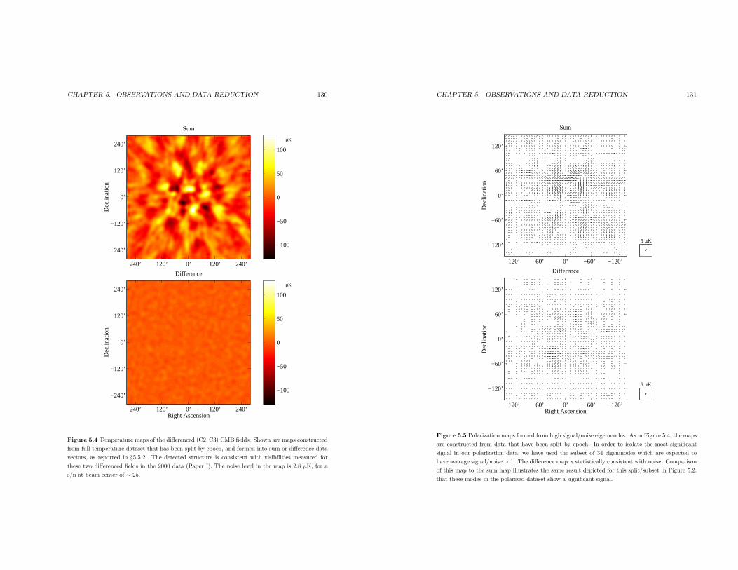
CHAPTER 5. OBSERVATIONS AND DATA REDUCTION 130
−100
−50
0
50
100
Dec
linat
ion
Sum
µK
−240’−120’0’120’240’
−240’
−120’
0’
120’
240’
−100
−50
0
50
100
Right Ascension
Dec
linat
ion
Difference
µK
−240’−120’0’120’240’
−240’
−120’
0’
120’
240’
Figure 5.4 Temperature maps of the differenced (C2–C3) CMB fields. Shown are maps constructed
from full temperature dataset that has been split by epoch, and formed into sum or difference data
vectors, as reported in §5.5.2. The detected structure is consistent with visibilities measured forthese two differenced fields in the 2000 data (Paper I). The noise level in the map is 2.8 µK, for a
s/n at beam center of ∼ 25.
CHAPTER 5. OBSERVATIONS AND DATA REDUCTION 131
−120’−60’0’60’120’
−120’
−60’
0’
60’
120’
Dec
linat
ion
Sum
5 µK
−120’−60’0’60’120’
−120’
−60’
0’
60’
120’
Right Ascension
Dec
linat
ion
Difference
5 µK
Figure 5.5 Polarization maps formed from high signal/noise eigenmodes. As in Figure 5.4, the maps
are constructed from data that have been split by epoch. In order to isolate the most significant
signal in our polarization data, we have used the subset of 34 eigenmodes which are expected to
have average signal/noise > 1. The difference map is statistically consistent with noise. Comparison
of this map to the sum map illustrates the same result depicted for this split/subset in Figure 5.2:
that these modes in the polarized dataset show a significant signal.

CHAPTER 5. OBSERVATIONS AND DATA REDUCTION 132
difference data vectors of the epoch split temperature data. The sum map clearly
shows structure enveloped by the primary beam, and as expected from the χ2 tests,
no residual signal is seen in the difference map above the noise. The detected structure
is consistent with visibilities measured for these two differenced fields in the 2000 data
presented in Paper I. With a noise floor in the difference map of 2.8 µK, we achieve
a s/n ratio of approximately 25 at beam center. Natural (inverse noise) weighting of
the full set of visibilities has been used, for a synthesized beam of ∼ 22′.
The polarization map shown in Figure 5.5 gives a visual representation of the
repeatable polarization signal. Shown are the epoch split sum and difference polar-
ization maps, constructed using the same s/n > 1 modes of the polarization data in
the concordance model s/n eigenmode basis that appear in the table and in Figure 5.2.
Because the maps have only 34 independent modes, they exhibit a limited range of
morphologies. Also, the formation of the s/n modes selects linear combinations of
visibilities which interfere constructively in the primary beam. Therefore, although
the same direct Fourier transform mapping algorithm is used, a beam taper is intrin-
sic to these modes (see Figure 5.3). This taper is evident in the difference map even
though it is statistically consistent with noise. Comparison of the level of structure
in this map and in the sum map illustrates the result of the χ2 analyses: that these
individual modes in the polarized dataset show a significant repeatable signal.
5.6.2 Significance
It is possible to calculate a similar χ2 statistic for the data vector formed from the
complete, unsplit dataset. Combining all the data without the requirement of forming
two equally weighted subsets should yield minimal noise, albeit without an exactly
corresponding null (i.e., difference) test. Recalculating the s/n eigenmodes for this
complete cross-polar data vector gives 36 modes with expected s/n > 1, for which
χ2 = 98.0 with a PTE = 1.2×10⁻⁷. This significance is similar to those from the sum
data vectors under the various splits, which actually divide the data fairly equally
CHAPTER 5. OBSERVATIONS AND DATA REDUCTION 133
and so are nearly optimal.
It should be noted that our focus so far has been examining the cross-polar data
for a signal in excess of the instrumental noise model. We have not addressed the
small cross-polar signal expected due to off-axis leakage of the temperature signal.
As discussed in §4.5, it is not possible to correct the data elements directly for this
effect, but we can account for it in calculating these χ2 results by including the
expected covariance of this leakage signal (see §??) in the noise matrix CN . Again
recalculating the s/n eigenmodes, we find 34 cross-polar modes with s/n > 1 which
give a χ2 = 97.0 and a PTE = 5.7 × 10⁻⁸, a significance which is similar to before.
The off axis leakage is also included in the likelihood analyses, where it again is found
to have an insignificant impact on the results.
The likelihood analysis described in the next chapter makes use of all of the
information in our dataset. Such an analysis, in principle, may yield statistically
significant evidence of a signal even in cases of datasets for which it is not possible to
isolate any individual modes which have average s/n > 1. However, the existence of
such modes in our dataset, which has resulted from our strategy of integrating deeply
on a limited patch of sky, allows us to determine the presence of the signal with the
very simple analysis described above. It also reduces sensitivity to the noise model
estimation in the likelihood results that we report next. Finally, it gives our dataset
greater power to exclude the possibility of no signal than it might have had if we had
observed more modes but with less s/n in each.

Chapter 6
Likelihood Analysis
The preceding chapter reported strong evidence for the presence of a signal in the
polarization dataset. The signal was determined to be a consistent feature of the
observations, and cannot be accounted for by instrumental noise. Our goal now is to
examine this signal, quantifying its strength and distribution within the dataset. We
wish to test, in as many different ways as the data will support, whether the signal
is consistent with the predicted signature of the density perturbation E-mode CMB
polarization expected under the standard model.
Our basic statistical tool for constructing these tests will be likelihood analy-
sis. The relatively manageable size of the DASI polarization dataset makes a direct
likelihood-based approach feasible, and we present results from nine separate such
analyses. The first portion of this chapter describes the methods for computing the
likelihoods of the various models of the signal that we explore in the analyses. The
different choices of parameterization of the CMB spectra in each analysis and the
corresponding parameter window functions are discussed, as well as details of our
conventions for reporting results.
Next we present the results themselves, organized first into those analyses that use
only the polarization data to constrain the E- and B-spectra, followed by analyses
of only the temperature data, and finally joint analyses using all of the data to
constrain the cross spectra. We conclude the chapter with a discussion of the level
134
CHAPTER 6. LIKELIHOOD ANALYSIS 135
of uncertainty due to various instrumental effects or the contribution of foregrounds
which could impact these results.
6.1 Likelihood Analysis Formalism
We begin our analysis by considering the data vector to be the sum of signal and
noise components,
∆ = s+ n, (6.1)
which are assumed to be independent and Gaussian distributed with zero mean. Thus
the covariance matrix of the data can be written
C = CT +CN , (6.2)
and gives a complete statistical description of the information content of our dataset.
The noise covariance matrix CN ≡ 〈nnt〉, is computed internally from the timestream
data and subjected to extensive consistency tests (see §5.5). It is regarded as the
known component of the covariance.
The theory covariance CT ≡ 〈sst〉 depends on the the two-point statistics of the
CMB temperature and polarization signals on the sky, which are specified by the T ,
E, and B power spectra and cross spectra. The theory covariance matrix is modeled
in terms of parameters κ which specify these spectra. For most analyses, we choose
parameters such that the full theory covariance matrix is the sum of components
proportional to each parameter,
CT (κ) =∑
p
κpBpT . (6.3)
In chapter 2 we derived a general expression for components of the theory covariance
matrix based on the temperature and polarization response of the visibilities which

CHAPTER 6. LIKELIHOOD ANALYSIS 136
make up the DASI dataset. From Eq.2.19 we can write
BpT ij =
1
2αiαj
∫du CX (u) A (ui − u, νi)
×[ξ1A (uj − u, νj) + ξ2A (uj + u, νj)
]. (6.4)
In this expression the autocorrelation of the aperture field A (u, νi) specifies the
beam pattern at frequency νi, αi = ∂BPlanck (νi, TCMB) /∂T converts from units
of CMB temperature to flux density (Jy), and the coefficients ξ1 and ξ2 take
values 0,±1,±2 × cos 2χ, 4χ , sin 2χ, 4χ depending on the Stokes states
(RR,LL,RL,LR) and selection of real or imaginary visibility for each of the two
baselines i, j and on which of the six spectra (T,E,B, TE, TB,EB) is specified by
X. For each parameter κp, the integration may be limited to annular regions which
correspond to l−ranges over which the power spectrum CX is hypothesized to be
relatively flat, or else some shape of the spectrum may be postulated (see §6.1.1).With this parametrized model for the covariance of the signal, we write our model
for the full covariance matrix of the data
C (κ) ≡ CT (κ) +CN . (6.5)
The likelihood of the model specified by the parameter vector κ is the probability of
obtaining our data vector ∆ given that model:
L (κ) = P (∆|κ)
= (2π)−N/2 det (C (κ))−1/2 exp
(−1
2∆tC (κ)−1∆
). (6.6)
Although the full likelihood function itself, defined over the parameter space explored,
is the most fundamental result of each of our likelihood analyses, it is useful to
identify and report the values of the parameters that maximize the likelihood (so-
called maximum likelihood (ML) estimators). These are often interpreted as the most
likely values of those parameters within the context of a given model, given a uniform
prior in our knowledge of the parameters. Uncertainties in the parameter values can
CHAPTER 6. LIKELIHOOD ANALYSIS 137
be estimated by characterizing the shape of the likelihood surface, as discussed further
in §6.1.7.The likelihood function allows us directly to compare the compatibility of our
dataset with any of the models in the considered parameter space, including those that
represent the predicted CMB polarization signal, or radically different polarization
signals, or no polarization at all. It is a particularly appropriate tool for the purposes
of our current analysis, in which we hope to establish an initial detection of the CMB
polarization and to examine whether the observed signal matches the expected one.
Indeed, the likelihood approach was originally advocated for CMB analysis (see, for
example, Readhead et al. (1989)) to address similar goals among early temperature
anisotropy experiments.
An alternative to the likelihood approach is to form parameter estimates directly
as quadratic functions of the data,
κp =∆tQp∆− bp , (6.7)
where the matrices Qp and constants bp are constructed using knowledge of CN and
an assumed CT (κ) based on an initial guess at parameter values κ (see Tegmark
& de Oliveira-Costa (2001) for an overview of this approach applied to polarization
data). Appropriately constructed quadratic estimators can be shown, if the initial
guess at parameter values is close to the true model, to offer minimum variance es-
timates of parameter values (Tegmark 1997b) and have the advantages that they
can be applied to the data in n2 operations (while the matrix inversion in evaluat-
ing the likelihood scales as n3) and that their error properties are easily expressed
analytically. Indeed, an iterated quadratic estimator quickly converges in parameter
space to the ML estimator (Bond et al. 1998), offering an efficient algorithm for use
in likelihood evaluation (see §6.1.2 and 6.1.5) rather than a distinct approach. The
use of non-iterated quadratic estimators as an alternative to likelihood analysis for

CHAPTER 6. LIKELIHOOD ANALYSIS 138
power spectrum estimation has gained popularity among recent temperature map-
ping experiments as larger datasets make direct likelihood evaluation prohibitive. As
future polarization experiments map more sky and move beyond the stage of initial
detections to precise power spectrum measurements, this pattern is likely to be re-
peated, and a great deal of recent literature has focused on the construction of E, B,
and cross spectra polarization quadratic estimators under various assumptions about
sky coverage, etc. (for examples, see Tegmark & de Oliveira-Costa (2001), ?, Chon
et al. (2003)). For our current dataset, however, exploring the full likelihood function
is practical and offers the most complete picture of the information our data holds
about CMB polarization.
6.1.1 Likelihood Parameters
In §6.2 we present the results from nine separate likelihood analyses involving the
polarization data, the temperature data, or both. Our choice of parameters with
which to characterize the six CMB power spectra in constructing CT (κ) is a compro-
mise between maximizing sensitivity to the signal and constraining the shape of the
power spectra. In the different analyses we either characterize various power spectra
with a single amplitude parameter covering all angular scales, or split the l−rangeinto five bands over which spectra are approximated as piecewise-flat, in units of
l(l + 1)Cl/(2π). Five bands were chosen as a compromise between too many for the
data to bear and too few to capture the shape of the underlying power spectra. The
l−ranges of these five bands are based on those of the nine-band analysis of Paper
II; we have simply combined the first four pairs of these bands, and kept the ninth
as before. In some analyses we also constrain the frequency spectral indices of the
temperature and polarization power spectra as a test for foreground contamination.
The l−range to which DASI has non-zero sensitivity is 28 < l < 1047. That range
includes the first three peaks of the temperature power spectrum, and within it the
amplitude of that spectrum, which we express in units l(l + 1)Cl/(2π), varies by a
CHAPTER 6. LIKELIHOOD ANALYSIS 139
factor of ∼ 4. Over this same range, the E-mode polarization spectrum is predicted to
have four peaks while rising roughly as l2 (in the same units), varying in amplitude by
nearly two orders of magnitude (Hu & White 1997). The TE correlation is predicted
to exhibit a complex spectrum that in fact crosses zero five times in this range.
Single bandpower analyses offer the clearest statistics to test for a potential sig-
nal, but the shape of the model power spectrum assumed will have an effect on the
sensitivity of the result. In particular, if the assumed shape is a poor fit to the true
spectrum preferred by the data, the results will be both less powerful and difficult to
interpret. For temperature spectrum measurements, the most common choice in re-
cent years has been the so-called flat bandpower, l(l+1)Cl ∝ constant, which matches
the gross large-angle “scale-invariant” power law shape of that spectrum. Because
of extreme variations predicted in the E and TE spectra over DASI’s l−range, wedo not expect a single flat bandpower parameterization to offer a good description of
the entire dataset (although in §6.2.1 we describe results of applying such an analysis
to limited l-range subsets of data). A more appropriate definition of “flat band-
power” for polarization measurements sensitive to large ranges of l < 1000 might be
Cl ∝ constant (or l(l+1)Cl ∝ l2). Other shapes have been tried, notably the Gaussian
autocorrelation function (by the PIQUE group (Hedman et al. 2001)) which reduces
to Cl ∝ constant at large scales and perhaps offers a better fit to the gross amplitude
of the predicted E spectrum than simple power laws.
In our single band analyses, we have chosen a shape for our single bandpower
parameters based on the predicted spectra for a cosmological model currently favored
by observations. The specific model that we choose—which we will call the concor-
dance model—is a ΛCDM model with flat spatial curvature, 5% baryonic matter,
35% dark matter, 60% dark energy, and a Hubble constant of 65 km s−1 Mpc−1,
(Ωb = 0.05,Ωcdm = 0.35,ΩΛ = 0.60, h = 0.65) and the exact normalization
C10 = 700µK2. As discussed in Chapter 1, this concordance model was defined
in Paper III as a good fit to the 2000 DASI temperature power spectrum and other

CHAPTER 6. LIKELIHOOD ANALYSIS 140
observations. The concordance model spectra for T , E, and TE are shown in Fig-
ure 6.6. The five flat bandpower likelihood results shown in the same figure, and
discussed in that section, suggest that the concordance shaped spectra do indeed bet-
ter characterize the data than any power-law approximation. In §6.2.1, we explicitly
test the likelihood of the concordance model parameterization against that of the two
power laws mentioned above, and find that the concordance model shape is strongly
preferred by the data.
6.1.2 Parameter window functions
It should be noted that the likelihood analysis is always model dependent, regard-
less of whether flat bandpowers or a shaped model is chosen for parameterization.
To evaluate the expectation value of the results for a hypothesized theoretical power
spectrum, one must use window functions appropriate for the parameters of the par-
ticular analysis.
The calculation of such parameter window functions has been given in the liter-
ature in the context of flat bandpower parameters in temperature power spectrum
likelihood analyses (Knox 1999; Halverson 2002), and for arbitrary quadratic estima-
tors of polarization spectra (Tegmark & de Oliveira-Costa 2001). These derivations
are equivalent if a minimum variance quadratic estimator which converges to the ML
estimate is chosen. Following the latter, a generic quadratic estimator (Eq. 6.7) has
the expectation value
〈κp〉 =⟨Tr(Qp∆∆
t)⟩− bp
= Tr (QpCT ) + Tr (QpCN)− bp
=∑
X,l
CXl Tr
(QpB
X,lT
). (6.8)
where we have chosen bp to cancel the noise term in the second line. In the third line
we have expanded CT as in Eqs. 6.3 and 6.4, using the actual multipole values of the
CHAPTER 6. LIKELIHOOD ANALYSIS 141
six power spectra CXl as our parameters (or approximating this with finely spaced
bandpowers). This expression implicitly defines the window function
(WXl )p ≡ Tr
(QpB
X,lT
)(6.9)
which gives the sensitivity of our parameter estimate κp to each of the underlying
power spectra.
Our specific quadratic estimator is constructed using the Fisher matrix, which is
defined to be the ensemble average of the curvature of the log likelihood
Fpp′(κ) ≡ −⟨∂2 lnL
∂κp∂κp′
⟩=
1
2Tr
(C−1∂CT
∂κpC−1∂CT
∂κp′
). (6.10)
Note that this matrix, which offers an estimate of the paramter uncertainties, is
calculated with reference to specific parameter values κ but does not depend on the
data. We define the estimator
Qp ≡1
2
∑
p′
(F−1
)pp′C−1∂CT
∂κp′C−1 . (6.11)
Iteration of this estimator approximates the Newton-Raphson method for maximizing
the likelihood (Bond et al. 1998). Starting near the true parameter values, then, its
expectation value approximates the ML estimate. From Eq. 6.9, the corresponding
parameter window function is
(WXl )p =
∑
p′
(F−1
)pp′
1
2Tr
(C−1∂CT
∂κp′C−1BX,l
T
). (6.12)
This expression is equivalent to the flat band-power window function defined in
Halverson (2002), generalized to include response to all six power spectra with arbi-
trary parameterization.
In general, the parameter window function has a non-trivial shape (even for a flat
band-power analysis) which is dependent on the shape of the true spectra as well
as the intrinsic sensitivity of the instrument as a function of angular scale. Param-
eter window functions for the E/B and E5/B5 polarization analysis are shown in
Figure 6.1.

CHAPTER 6. LIKELIHOOD ANALYSIS 142
0
1
0 200 400 600 800 1000
0
1
norm
aliz
ed r
espo
nse
l (angular scale)
Figure 6.1 Parameter window functions, which indicate the angular scales over which the param-
eters in our analyses constrain the power spectra. The upper panel shows the functions for the
E parameter of our E/B analysis, with the solid blue curve indicating response to the E power
spectrum and the solid red (much lower) curve indicating response of the same E parameter to
the B spectrum. The blue dashed curve shows the result of multiplying the E window function
by the concordance E spectrum, illustrating that for this CMB spectrum, most of the response of
our experiment’s E parameter comes from the region of the second peak (300 . l . 450), with a
substantial contribution also from the third peak and a smaller contribution from the first. The
lower panel shows E1 – E5 parameter window functions for the E power spectrum (blue) and B
power spectrum (red, again much lower) from our E5/B5 analysis. All of these window functions
are calculated with respect to the concordance model discussed in the text. DASI’s response to E
and B is very symmetric, so that E and B parameter window functions which are calculated with
respect to a model for which E = B are similar, with the E and B spectral response reversed.
CHAPTER 6. LIKELIHOOD ANALYSIS 143
6.1.3 Point Source Constraints
The covariance matrix that we actually construct for our likelihood evaluation has
several components in addition to the standard noise and theory covariance terms of
Eq. 6.5.
Potentially contaminated modes in the data vector may be eliminated from the
analysis by the construction of constraint matrices (Bond et al. 1998). These matrices
attribute essentially infinite variance to selected modes, and when added to the noise
covariance matrix, they have the effect of assigning zero weight to these modes in the
likelihood evaluation. This constraint matrix formalism can be used to remove the
effect of point sources of known position without knowledge of their flux densities,
as described in Paper II and Halverson (2002). In generalizing this procedure to
include the case of polarized point sources, for each point source of known location
a constraint matrix can be constructed that projects out two additional modes from
the covariance matrix, corresponding to the unknown Q and U polarized flux of the
source.
Although we have tested for the presence of point sources in the polarization power
spectra using this method, in the final analysis we use constraint matrices to project
point sources out of the temperature data only, and not the polarization data (see
§6.3.2 for further discussion).
6.1.4 Off-axis Leakage Covariance
Another small correction to the covariance matrix for the polarization data results
from the off-axis leakage (see §4.5), which has the effect of mixing some power from the
temperature signal T near the edge of our fields into the cross-polar visibilities. Unlike
the on-axis leakage, the off-axis leakage cannot be calibrated out of the polarization
data baseline-by-baseline, but it can be accounted for in the theory covariance matrix.
Our aperture-plane model of the off-axis leakage field allows us write an expression

CHAPTER 6. LIKELIHOOD ANALYSIS 144
for the resulting covariance that has the same form as Eq. 6.4, but with the autocor-
relation of the usual aperture field A (u, νi) replaced by the convolution of this field
with the leakage field. An alternative is to derive the resulting covariance statisti-
cally from simulated observations of fields with a known input power spectrum CT
in which the polarized signal due to off-axis leakage has been calculated according to
our sky-plane model of this leakage. Because our data on the off-axis leakage is more
successfully fit by our sky-plane model, we adopt this latter approach, calculating
the off-axis leakage covariance due to concordance model temperature anisotropies
using 5000 simulated observations. For analyses in which the amplitude of CMB
temperature anisotropies is included as a parameter, the amplitude of this covariance
component is tied to that parameter; in polarization-only analyses it is fixed at the
concordance normalization. In either case, inclusion of off-axis leakage covariance has
only a small effect on likelihood results, as discussed in §6.3.
6.1.5 Likelihood Evaluation
Prior to likelihood analysis, the data vector and the covariance matrices can be com-
pressed by combining visibility data from nearby points in the (u, v) plane, where the
signal is highly correlated. This reduces the computational time required for the anal-
yses without a significant loss of information about the signal. Like the post-reduction
calibration operations described in the Chapter 5, compression is implemented as a
matrix operation applied to both the data vector and covariance matrices. Compres-
sion techniques ranging in complexity from simple frequency band combination, to
explicit uv-plane griding, to signal-to-noise eigenmode transformations were all found
to be useful at different stages of the analysis, and our final algorithm is based on it-
erative minimum-variance combination of those data elements with the highest signal
correlations, according to a fiducial theory matrix. All analyses were run on standard
CHAPTER 6. LIKELIHOOD ANALYSIS 145
desktop workstations. 1
For each analysis, we use the iterated quadratic estimator described in §6.1.2to find the ML values of our parameters. To further characterize the shape of the
likelihood function, in Paper II we used an offset log-normal approximation. Here,
for improved accuracy in calculating confidence intervals and likelihood ratios, we
explicitly map out the likelihood function by evaluating Equation 6.6 over a uniform
parameter grid large enough to enclose all regions of substantial likelihood. A single
likelihood evaluation typically takes several seconds, so this explicit grid evaluation is
impractical for the analyses which include five or more parameters. For each analysis
we also implement a Markov chain evaluation of the likelihood function (Christensen
et al. 2001). We find this to be a useful and efficient tool for mapping the likelihoods
of these high-dimensional parameter spaces in the region of substantial likelihood. We
have compared the Markov technique to the grid evaluation for the lower-dimensional
analyses and found the results to be in excellent agreement (see Figure 6.5). In all
cases, the peak of the full likelihood evaluated with either technique is confirmed to
coincide with the ML values returned by the iterated quadratic estimator.
6.1.6 Simulations and Parameter Recovery Tests
The likelihood analysis software was extensively tested through analysis of simulated
data. The data simulation software was authored independently of the analysis soft-
ware by a different member of our team (E. Leitch) as a precaution against shared
coding errors, and using this software, a number of “blind” parameter recovery tests
were performed.
Simulated sky maps were generated from realizations of a variety of smooth CMB
power spectra, including both the concordance spectrum and various non-concordance
models, both with and without E and B polarization and TE correlations. Multiple
1Our standard machines are Linux-based PC’s running 32-bit Intel Pentium processors at 1-2 GHz, with 2-6 GB of memory.

CHAPTER 6. LIKELIHOOD ANALYSIS 146
independent realizations of the sky were “observed” to construct simulated visibilities
with Fourier-plane sampling identical to the real data. The simulations were designed
to replicate the actual data as realistically as possible and include artifacts of the
instrumental polarization response and calibration, such as the on-axis and off-axis
leakages described in §4.4, and the cross-polar phase offset described in §??, allowingus to test the calibration operations and treatment of these effects implemented in
the analysis software.
Each of the analyses described in §6.2 was performed on hundreds of these simu-
lated datasets with independent realizations of sky and instrument noise, both with
noise variances that matched the real data, and with noise a factor of 10 lower. In
all cases, we found that the means of the ML estimators recovered the expectation
values 〈κp〉 of each parameter without evidence of bias, and that the variance of the
ML estimators was found to be consistent with the estimated uncertainty given by
F−1 evaluated at 〈κ〉, where F is the Fisher matrix (Eq. 6.10).
6.1.7 Reporting of Likelihood Results
Maximum likelihood parameter estimates reported in this paper are the global max-
ima of the multidimensional likelihood function. Confidence intervals for each param-
eter are determined by integrating (marginalizing) the likelihood function over the
other parameters; the reported intervals are the equal-likelihood bounds which enclose
68% of this marginal likelihood distribution. This prescription corresponds to what is
generally referred to as the highest posterior density (HPD) interval. An alternative
prescription, so-called central likelihood intervals which exclude equal amounts of in-
tegrated likelihood above and below the central 68%, is more sensitive to integration
over low-likelihood regions (and thus to implicit priors), and for the skewed likelihood
distributions typical of parameters that are physically positive generally gives inter-
vals shifted to somewhat higher values (see Fig. 6.5). When calculating the HPD
intervals we consider all parameter values, including non-physical ones, because our
CHAPTER 6. LIKELIHOOD ANALYSIS 147
aim is simply to summarize the shape of the likelihood function. Values are quoted
in the text using the convention “ML (HPD-low to HPD-high)” to make clear that
the confidence range is not directly related to the maximum likelihood value. Where
results are given in units of µK2, values are for l(l + 1)Cl/(2π).
In the tabulated results, we also report marginalized uncertainties obtained by
evaluating the Fisher matrix at the maximum likelihood model, i.e., (F−1)1/2pp for pa-
rameter p. Although in most cases, the two confidence intervals are quite similar,
we report the HPD interval as the primary result, as it offers more information on
the shape of the likelihood function. The scatter of ML estimators returned in mul-
tiple simulations is verified to be consistent with the expected uncertainty given by
F−1 evaluated at the true input model. Note that this is not necessarily the same
uncertainty derived by evaluating F−1 at the ML estimates, which can give much
smaller apparent “error-bars” if a power estimate has fluctuated to a low value for a
particular simulation.
For parameters which are intrinsically positive we consider placing (physical) up-
per limits by marginalizing the likelihood distribution as before, but excluding the
unphysical negative values. We then test if the 95% integral point has a likelihood
smaller than that at zero; if it does we report an upper limit in addition to a confidence
interval.
We also report the parameter correlation matrices for our various likelihood anal-
yses to allow the reader to gauge the degree to which each parameter has been deter-
mined independently. The covariance matrix is the inverse of the Fisher matrix and
the correlation matrix is defined as the covariance matrix normalized to unity on the
diagonal, i.e., C = F−1 and Rij = Cij/√CiiCjj.
6.1.8 Goodness-of-Fit Tests
One of the primary goals of our analysis is to determine if our results are consistent
with a given model. For example, we would like to examine the significance of any

CHAPTER 6. LIKELIHOOD ANALYSIS 148
detections by testing for the level of consistency with zero signal models, and we
would like to determine if the polarization data are consistent with predictions of the
standard cosmological model. These questions are in a sense more basic than the
problem of parameter estimation, and we can use the likelihood function to directly
address them.
We define as a goodness-of-fit statistic the logarithmic ratio of the maximum of
the likelihood to its value for some model H0 described by parameters κ0.
Λ(H0) ≡ − log
(L (κML)
L (κ0)
).
The statistic Λ simply indicates how much the likelihood has fallen from its peak value
down to its value at κ0. Large values indicate inconsistency of our data’s likelihood
result with the model H0. To assess significance, we perform Monte Carlo (MC)
simulations of this statistic under the hypothesis that H0 is true. From this, we can
determine the probability, given H0 true, to obtain a value of Λ that exceeds the
observed value, which we hereafter refer to as PTE.
When considering models which the data indicate to be very unlikely, i.e., for
which Λ is large, sufficient MC sampling of the distribution of this statistic becomes
computationally prohibitive; our typical MC simulations are limited to only 1000
realizations. In the limit that the parameter errors are normally distributed, our
chosen statistic reduces to Λ = ∆χ2/2. The integral over the χ2 distribution is
described by an incomplete gamma function;
PTE =1
Γ(N/2)
∫ ∞
Λ
e−xxN2−1dx
where Γ(x) is the complete gamma function, and N is the number of parameters.
Neither the likelihood function nor the distribution of the ML estimators is, in
general, normally distributed, and therefore this approximation must be tested. In
all cases where we can compute a meaningful PTE with MC simulations, we find it
to be in excellent agreement with the analytic approximation, justifying its adoption.
CHAPTER 6. LIKELIHOOD ANALYSIS 149
All results for PTE based on the likelihood ratio statistic are calculated using this
analytic expression unless otherwise stated. In multiparameter analyses where we
are interested in the goodness-of-fit of a single parameter or subset of parameters,
we form a Λ statistic and PTE for the reduced parameter set after marginalizing the
likelihood function over the other parameters.
6.2 Likelihood Results
In the following sections we discuss the nine separate likelihood analyses we have
conducted, first dealing with analyses based on our polarization data only, then those
based on temperature data only, and finally joint temperature-polarization analyses.
Final numerical results for the three groups of analyses are given in Tables 6.1, 6.2
and 6.3, on pages 160, 162 and 167, respectively.
6.2.1 Polarization Data Analyses and E and B Results
E/B analysis
The E/B analysis uses two single bandpower parameters to characterize the am-
plitudes of the E and B polarization spectra. As discussed in §6.1.1, this analysis
requires a choice of shape for the spectra to be parameterized. DASI has instrumental
sensitivity to E and B that is symmetrical and nearly independent. Although the B
spectrum is not expected to have the same shape as the E spectrum, is expected to
have negligible amplitude. We choose the same shape for both spectra in order to
preserve this symmetry in the analysis.
We first compute the likelihood using a bandpower with l(l+1)Cl/2π = constant
(“flat” bandpower) including data only from a limited l range in which DASI has high
sensitivity, as seen in Figure 6.1. Using the range 300 < l < 450 which includes 24%
of the complete dataset, we find the ML at flat bandpower values E = 26.5µK2 and

CHAPTER 6. LIKELIHOOD ANALYSIS 150
0
10
20
30
E (
µK2 )
−10
0
10
B (
µK2 )
250 300 350 400 450 500
1
2
3
4
5
6
l (angular scale)
"sig
ma"
Figure 6.2 Results from E/B flat bandpowers computed on restricted ranges of data. A “flat”
bandpower analysis using only baselines in the range 300 < l < 450, which includes 24% of the com-
plete dataset and covers the angular scales at which DASI is expected to have greatest polarization
sensitivity, gives likelihoods that peak at E = 26.5µK2 and B = 0.8µK2, with a significance of E
detection of 5.8σ. These results are quite sensitive to the choice of this range, however, leading us to
seek a well motivated bandpower shape with which to perform the analysis over the entire l range
sampled by DASI.
B = 0.8µK2. The likelihood falls dramatically for the zero polarization nopol model
E = 0, B = 0. Marginalizing over B, we find Λ(E = 0) = 16.9 which, assuming
the uncertainties are normally distributed, corresponds to a PTE of 5.9 × 10⁻⁹ or
a significance of E detection of 5.8σ. As expected, changing the l range affects the
maximum likelihood values and the confidence of detection. This is illustrated in
Figure 6.2, in which it can be seen that shifting the center of the above l range by
±25 reduces the confidence of detection to 5.6σ and 4.8σ, respectively. Clearly it is
CHAPTER 6. LIKELIHOOD ANALYSIS 151
0 200 400 600 800 10000
10
20
30
40
50
E (
µK2 )
l (angular scale)
Figure 6.3 Comparison of concordance and two power-law spectrum shapes examined as candidates
for single parameter E/B analysis. All three are illustrated at the E spectrum amplitudes which
produced maximum likelihoods for each shape, but the likelihood of the best-fit model with a
concordance shape (green) is a factor of 200 and 12,000 higher than those of the l(l + 1)Cl ∝ l2
(blue) and l(l + 1)Cl ∝ constant (red, “flat”) cases, respectively.
desirable to perform the analysis over the entire l range sampled by DASI using a
well motivated bandpower shape for the parameterization.
We considered three a priori shapes to check which is most appropriate for our
data: the concordance E spectrum shape (as defined in §6.1.1), and two power law
alternatives, l(l+ 1)Cl ∝ constant (“flat”) and l(l+ 1)Cl ∝ l2 (see Fig. 6.3). For any
of these shapes, the point at E = 0, B = 0 corresponds to the same zero-polarization
nopolmodel, so that the likelihood ratios Λ(nopol) may be compared directly to assess
the relative likelihoods of the best-fit models. For the flat l(l+ 1)Cl ∝ constant case,
the ML flat bandpower values are E = 6.8µK2, B = −0.4µK2, with the log-likelihood
at zero falling by a factor of Λ(nopol) = 4.34. For the l(l + 1)Cl ∝ l2 case, the ML
values are E = 5.1µK2, B = 1.2µK2 (for values of l(l + 1)Cl/2π at l = 300), with
Λ(nopol) = 8.48. For the concordance shape, the ML values are E = 0.80, B = 0.21
in units of the concordance E spectrum amplitude, with Λ(nopol) = 13.76. The
likelihood of the best fit model in the concordance case is a factor of 200 and 12,000

CHAPTER 6. LIKELIHOOD ANALYSIS 152
higher than those of the l(l+ 1)Cl ∝ l2 and l(l+ 1)Cl ∝ constant cases, respectively;
compared to the concordance shape either of these is a very poor model for the data.
The data clearly prefer the concordance shape, which we therefore use for the E/B
and other single bandpower analyses presented in our results tables.
Figure 6.4 illustrates the result of the final E/B polarization analysis, using the
concordance shape. The maximum likelihood value of E is 0.80 (0.56 to 1.10 at 68%
confidence). For B, the result should clearly be regarded as an upper limit; 95% of
the B > 0 likelihood (marginalized over E) lies below 0.59.
The upper panel of Figure 6.1 shows the parameter window functions relevant for
this analysis. Note that the E parameter has very little sensitivity to B and vice
versa — as discussed in Chapter 2, the purity with which DASI can separate these
is remarkable. This separation is also demonstrated by the low correlation (−0.046)between the E and B parameters (see Table 6.1).
The likelihood of the zero polarization model (E=0, B=0) is 1.1×10⁻⁶ that of the
ML model, corresponding to Λ(nopolarization) = 13.76 as mentioned above. Using
the Monte Carlo method (§6.1.8) we find that in 1000 simulations with no polarization
the largest value of this Λ statistic obtained is 6.4 — far less than the observed value.
Assuming that the uncertainties in E and B are normally distributed (§6.1.8), thelikelihood ratio Λ(nopol) = 13.76 implies a probability that our data are consistent
with the zero polarization hypothesis of PTE = 1.05 × 10⁻⁶. We conclude that the
data are highly incompatible with the no polarization hypothesis. Marginalizing over
B, we find Λ(E = 0) = 12.1 corresponding to detection of E-mode polarization at a
PTE of 8.46× 10⁻⁷ (or a significance of 4.92σ).
The likelihood ratio for the concordance model gives Λ(E = 1, B = 0) = 1.23, for
which the Monte Carlo and analytic PTE are both 0.28. We conclude that our data
are consistent with the concordance model.
However, given the precision to which previous measurements have determined
the temperature power spectrum of the CMB, even within the ∼ 7 parameter class
CHAPTER 6. LIKELIHOOD ANALYSIS 153
0 0.5 1 1.5 2
0
0.5
1
1.5
2
E
B
E
likel
ihoo
d
0 0.5 1 1.5 20
0.5
1
0 0.5 1 1.5 20
0.5
1
B
likel
ihoo
d
Figure 6.4 Results from the two parameter shaped bandpower E/B polarization analysis. An
E-mode power spectrum shape as predicted for the concordance model is assumed, and the units
of amplitude are relative to that model. The same shape is assumed for the B-mode spectrum.
(right panel) The point shows the maximum likelihood value with the cross indicating Fisher matrix
errors. Likelihood contours are placed at levels exp(−n2/2), n = 1, 2..., relative to the maximum,i.e., for a normal distribution, the extrema of these contours along either dimension would give the
marginalized n-sigma interval. (left panels) The corresponding single parameter likelihood distri-
butions marginalized over the other parameter. Note the steep fall in likelihood toward low power
values; this likelihood shape (similar to a χ2 distribution) is typical for positive-definite parameters
for which a limited number of high signal/noise modes are relevant. The gray lines enclose 68% of
the total likelihood. The red line indicates the 95% confidence upper limit on B-mode power. The
green band shows the distribution of E expectation values for a large grid of cosmological models
weighted by the likelihood of those models given our previous temperature result (see text).

CHAPTER 6. LIKELIHOOD ANALYSIS 154
0 0.5 1 1.5 2
0
0.5
1
1.5
2
E
B0 0.5 1 1.5 2
0
0.5
1
E
likel
ihoo
d
0 0.5 1 1.5 20
0.5
1
B
likel
ihoo
d
Figure 6.5 Results from the same shaped bandpower E/B polarization analysis of Fig. 6.4 with
the likelihood calculated using a Markov chain, rather than an explicit grid evaluation. The Markov
chain technique (Christensen et al. 2001) is illustrated with a 3000 point chain in the right panel.
Unless a procedure is used to progressively rescale the definition of likelihood, the Markov chain does
not effectively map low likelihood (> 3σ) regions, and we prefer to rely on explicit grid evaluation in
our low-dimensional analyses (< 5 parameters) where it is practical. In the regions of high likelihood,
the techniques give identical results: 68% intervals derived from the Markov chain, illustrated for
each parameter in the left panels, match the corresponding intervals from explicit grid evaluation
to 1%. In addition to the 68% HPD intervals (solid gray lines) which we quote in our results, also
illustrated are 68% “central likelihood” intervals (dotted lines) which are sometimes used, and which,
due to the skewness of these distributions, tend to give higher power estimates.
of cosmological models often considered, the shape and amplitude of the predicted
E-mode spectrum are still somewhat uncertain. To quantify this, we have taken the
model grid generated for Paper III and calculated the expectation value of the shaped
band E parameter for each model using the window function shown in Figure 6.1. We
then take the distribution of these predicted E amplitudes, weighted by the likelihood
of the corresponding model given our previous temperature results (using a common
CHAPTER 6. LIKELIHOOD ANALYSIS 155
calibration uncertainty for the DASI temperature and polarization measurements).
This yields a 68% credible interval for the predicted value of the E parameter of 0.90
to 1.11. As illustrated in the upper left panel of Figure 6.4, our data are compatible
with the expectation for E based on existing knowledge of the temperature spectrum
and the standard model of CMB physics.
E5/B5 analysis
The top two panels of Figure 6.6 show the results of a ten parameter analysis char-
acterizing the E and B-mode spectra using five flat bandpowers for each. The lower
panel of Figure 6.1 shows the corresponding parameter window functions. Note the
extremely small uncertainty in the measurements of the first bands E1 and B1.
To test whether these results are consistent with the concordance model, we calcu-
late the expectation value for the nominal concordance model in each of the 5 bands,
yielding E=(0.8,14,13,37,16) and B=(0,0,0,0,0) µK2. The likelihood ratio comparing
this point in the ten dimensional parameter space to the maximum gives Λ = 5.1,
which for ten degrees of freedom results in a PTE of 0.42, indicating that our data
are consistent with the expected polarization parameterized in this way. The E5/B5
results are highly inconsistent with the zero polarization nopol hypothesis, for which
Λ = 15.2 with a PTE = 0.00073.
While quite significant, the PTE for this statistic is considerably weaker than the
equivalent one obtained for the single band analysis of §6.2.1due to the higher num-
ber of degrees of freedom in this analysis. In this ten dimensional space, all possible
random deviations from the nopol expectation values E=(0,0,0,0,0), B=(0,0,0,0,0)
are treated equally in constructing the PTE for our Λ statistic. Imagining the nopol
hypothesis to be true, it would be far less likely to obtain a result in this large pa-
rameter space that is both inconsistent with nopol at this level and at the same time
is consistent with the concordance model, than it would be to obtain a result that

CHAPTER 6. LIKELIHOOD ANALYSIS 156
0
2000
4000
6000
8000
T (
µK2 )
−50
0
50
100
E (
µK2 )
−50
0
50
100
B (
µK2 )
0 200 400 600 800 1000−200
−100
0
100
200
TE
(µK
2 )
l (angular scale)
Figure 6.6 Results from the five-band likelihood analyses. The ten parameter E5/B5 polarization
analysis is shown in the top two panels. The T5 temperature analysis is shown in the third panel.
The 5 TE bands from the T/E/TE5 joint analysis are shown in the bottom panel. All the results
are shown in flat bandpower units of l(l+1)Cl/2π. The blue line shows the piecewise flat bandpower
models representing the maximum likelihood parameter values, with the error bars indicating the
68% central region of the likelihood of each parameter, marginalizing over the other parameter values
(errors for E and B in the first band are too small to see clearly here). The green line shown for
each of the spectra is the concordance model.
CHAPTER 6. LIKELIHOOD ANALYSIS 157
0 0.5 1 1.5 2−5
−4
−3
−2
−1
0
1
2
3
4
5
E
spec
tral
inde
x0 0.5 1 1.5 20
0.5
1
E
likel
ihoo
d
−4 −2 0 2 40
0.5
1
spectral index
likel
ihoo
d
Figure 6.7 Results of E/betaE polarization shaped bandpower amplitude/spectral-index analyses.
The layout of the plot is analogous to Figure 6.4. The concordance power spectrum shape is assumed
for E, and in this analysis the B spectrum is set to zero. The spectral index is relative to the CMB,
so that 0 corresponds to a 2.73 K Planck spectrum. In these units synchrotron emission would be
expected to have an index of approximately −3.
is merely inconsistent with nopol in some way at this level. It is the latter proba-
bility that is measured by the PTE for our Λ(nopol), explaining why this approach
to goodness-of-fit weakens upon considering increasing numbers of parameters. One
could define a goodness-of-fit statistic that overcomes this limitation by making ex-
plicit reference to compatibility with the concordance-expectation-value model, for
example by examining the likelihood ratio between this model and the nopol model.
However, if one is willing to make reference to the concordance model in this way,
it is certainly preferable to use the actual concordance power spectrum shape rather
than a five-band approximation to it, which is exactly what the goodness-of-fit from
the single band E/B analysis of the previous section accomplishes.

CHAPTER 6. LIKELIHOOD ANALYSIS 158
0 0.5 1 1.5 2
−20
−15
−10
−5
0
5
10
15
20
25
30
35
Scalar
Ten
sor0 0.5 1 1.5 2
0
0.5
1
Scalar
likel
ihoo
d
−20 −10 0 10 20 300
0.5
1
Tensor
likel
ihoo
d
Figure 6.8 Results of Scalar/Tensor polarization analysis.
E/βE analysis
We have performed a two parameter analysis to determine the amplitude of the E-
mode polarization signal as above and the frequency spectral index βE of this signal
relative to the CMB (Figure 6.7). As expected, the results for the E-mode amplitude
are very similar to those for the E/B analysis described in the previous section. The
spectral index is found to be consistent with CMB: the maximum likelihood value
is βE = 0.17 (−1.63 to 1.92). Although the constraint is not strong, this result
nevertheless disfavors the domination of the polarization signal by foregrounds (see
§6.3.2 below).
Scalar/Tensor analysis
As discussed in Chapter 1, predictions exist for the shape of the E and B-mode spectra
which would result from primordial gravity waves, also known as tensor perturbations.
And although the amplitude of tensors is not well constrained by theory, they are
a generic prediction of inflation, and measurement of the tensor amplitude would
CHAPTER 6. LIKELIHOOD ANALYSIS 159
offer both a compelling confirmation of this remarkable theory and a direct probe
of the energy scale at which it occurred. In a concordance-type model including
tensors, their contributions to the polarization E and B spectra are expected to peak
at l ∼ 100. Assuming reasonable priors, current measurements of the temperature
spectrum (in which tensor and scalar contributions will be mixed) suggest T/S < 0.2
(Wang et al. 2002), where this amplitude ratio is defined in terms of the tensor
and scalar contributions to the temperature quadrupole CT2 . We use the distinct
polarization angular power spectra for the scalars (our usual concordance E shape,
with B = 0) and the tensors (which specify both ET and BT ) as two components of a
likelihood analysis to constrain the amplitude parameters of these components. This
analysis is illustrated in Figure 6.8.
In principle, because the scalar B-mode spectrum is zero this polarization-based
approach avoids the fundamental sample variance limitations arising from using the
temperature spectrum alone. For this reason, a great deal of future CMB polarization
experimental effort will be dedicated to constraining the tensor amplitude by targeting
these B-modes. However, the E5/B5 analysis (§6.2.1) indicates that DASI producesonly upper limits to the E and B−mode polarization at the angular scales most
relevant (l . 200) for the tensor spectra. It is therefore not surprising that our limits
on T/S derived from the polarization spectra as reported in Table 6.1 are quite weak.
6.2.2 Temperature Data Analyses and T Spectrum Results
T/βT analysis
Results are shown in Figure 6.9 for a two parameter analysis to determine the ampli-
tude and frequency spectral index of the temperature signal. The bandpower shape
used is that of the concordance T spectrum, and the amplitude parameter is ex-
pressed in units relative to that spectrum. As with the E/βE analysis, the spectral
index is relative to the CMB, so that 0 corresponds to a 2.73 K Planck spectrum.

CHAPTER 6. LIKELIHOOD ANALYSIS 160
(F−1
)1/2ii
68% interval 95%
parameter llow − lhigh ML est. error lower upper U.L. units
E/BE − 0.80 ±0.28 0.56 1.10 − frac. of concordance EB − 0.21 ±0.18 0.05 0.40 0.59 frac. of concordance EE5/B5E1 28− 245 -0.50 ±0.8 -1.20 1.45 2.38 uK2
E2 246− 420 17.1 ±6.3 11.3 31.2 − uK2
E3 421− 596 -2.7 ±5.2 -10.0 4.3 24.9 uK2
E4 597− 772 17.5 ±16.0 3.8 40.3 47.2 uK2
E5 773− 1050 11.4 ±49.0 -32.5 92.3 213.2 uK2
B1 28− 245 -0.65 ±0.65 -1.35 0.52 1.63 uK2
B2 246− 420 1.3 ±2.4 -0.7 5.0 10.0 uK2
B3 421− 596 4.8 ±6.5 -0.6 13.5 17.2 uK2
B4 597− 772 13.0 ±14.9 1.6 31.0 49.1 uK2
B5 773− 1050 -54.0 ±28.9 -77.7 -4.4 147.4 uK2
E/βEE − 0.84 ±0.28 0.55 1.08 − frac. of concordance EβE − 0.17 ±1.96 -1.63 1.92 − temp. spectral indexScalar/TensorS − 0.87 ±0.29 0.62 1.18 − frac. of concordance ST − -14.3 ±7.5 -20.4 -3.9 25.4 T/(S=1)
parameter correlation matrices
E B E βE S T1 −0.046 1 −0.082 1 −0.339
1 1 1
E1 E2 E3 E4 E5 B1 B2 B3 B4 B51 −0.137 0.016 −0.002 0.000 −0.255 0.047 −0.004 0.000 0.000
1 −0.117 0.014 −0.002 0.024 −0.078 0.004 0.000 0.0001 −0.122 0.015 −0.003 0.010 −0.027 0.003 −0.001
1 −0.119 0.000 −0.001 0.002 −0.016 0.0031 0.000 0.000 0.000 0.002 −0.014
1 −0.226 0.022 −0.002 0.0001 −0.097 0.011 −0.002
1 −0.111 0.0181 −0.164
1
Table 6.1 Results of the four likelihood analyses using polarization data only, described in §6.2.1.Each parameter set specifies a different prescription for the E and B polarization signals, in units
explained in the text. Definitions of the confidence intervals, Fisher matrix uncertainties, and upper
limits listed are given in §6.1.7.
CHAPTER 6. LIKELIHOOD ANALYSIS 161
0.5 1 1.5 2−1.5
−1
−0.5
0
0.5
1
1.5
T
spec
tral
inde
x0.5 1 1.5 20
0.5
1
T
likel
ihoo
d
−1 −0.5 0 0.5 10
0.5
1
spectral index
likel
ihoo
d
Figure 6.9 Results of T/betaT temperature shaped bandpower amplitude/spectral-index analyses.
The layout of the plot is analogous to Figure 6.7. The concordance power spectrum shape is assumed
for T , and spectral index is relative to the CMB blackbody. Determination of the spectral index
of the observed temperature signal, unlike its power, is not limited by sample variance, so that
significant unpolarized foreground contamination can be ruled out to high precision.
The amplitude of T has a maximum likelihood value of 1.19 (1.09 to 1.30), and the
spectral index βT = −0.01 (−0.16 to 0.14). While the uncertainty in the temperature
amplitude is dominated by sample variance, the spectral index is limited only by
the sensitivity and fractional bandwidth (32%) of DASI. Due to the extremely high
signal/noise of the temperature data, the constraints on spectral index are superior
to those from previous DASI observations (Paper II), strictly limiting the degree of
unpolarized foreground contamination in these fields, as further discussed in §6.3.2.
T5 analysis
The third panel of Figure 6.6 shows the results of an analysis using five flat bands to
characterize the temperature spectrum. These results are completely dominated by
the sample variance in the differenced field. They are consistent with, although less

CHAPTER 6. LIKELIHOOD ANALYSIS 162
(F−1
)1/2ii
68% interval
parameter llow − lhigh ML est. error lower upper units
T/βTT − 1.19 ±0.11 1.09 1.30 fraction of concordance TβT − -0.01 ±0.12 -0.16 0.14 temperature spectral indexT5T1 28− 245 6510 ±1610 5440 9630 uK2
T2 246− 420 1780 ±420 1480 2490 uK2
T3 421− 596 2950 ±540 2500 3730 uK2
T4 597− 772 1910 ±450 1530 2590 uK2
T5 773− 1050 3810 ±1210 3020 6070 uK2
parameter correlation matrices
T1 T2 T3 T4 T5 T βT1 −0.101 0.004 −0.004 −0.001 1 0.023
1 −0.092 −0.013 −0.011 11 −0.115 −0.010
1 −0.1471
Table 6.2 Results of the two likelihood analyses using temperature data only, described in §6.2.2.Each parameter set specifies a different prescription for the temperature signal. Definitions of the
confidence intervals and Fisher matrix uncertainties listed are given in §6.1.7.
precise than our previous temperature power spectra described in Paper II; we include
them here primarily to emphasize that DASI makes measurements simultaneously in
all four Stokes parameters and is able to measure temperature as well as polarization
anisotropy.
The usual unpolarized point source constraints have been applied here and in all
other analyses of the temperature data. In addition, the temperature power spectrum
reported in Paper II included an adjustment to correct for the small power contri-
bution of point sources below the flux threshold of our constraints. This residual
point source correction is dependent on the point source population model and is
small compared to the uncertainties of the temperature results here; for simplicity it
is omitted in reporting the current results.
CHAPTER 6. LIKELIHOOD ANALYSIS 163
0 0.5 1 1.5 2−2
−1.5
−1
−0.5
0
0.5
1
1.5
2
E
TE
0 0.5 1 1.5 20
0.5
1
T
likel
ihoo
d
0 0.5 1 1.5 20
0.5
1
E
likel
ihoo
d
−2 −1 0 1 20
0.5
1
TE
likel
ihoo
d
Figure 6.10 Results from the 3 parameter shaped bandpower T/E/TE joint analysis. Spectral
shapes as predicted for the concordance model, are assumed and the units are relative to that model.
The layout of the plot is analogous to Figure 6.4. The two dimensional distribution in the right
panel is marginalized over the T dimension.
6.2.3 Joint Analyses and TE, TB, EB Cross Spectra Results
T/E/TE analysis
Figure 6.10 shows the results of a three parameter single bandpower analysis of the
amplitudes of the T and E spectra, and the TE cross correlation spectrum. As before,
bandpower shapes based on the concordance model are used. The T and E constraints
are, as expected, very similar to those from the E/B, E/βE and T/βT analyses

CHAPTER 6. LIKELIHOOD ANALYSIS 164
described above. The new result here is TE which has a maximum likelihood value
of 0.91 (0.45 to 1.37). Note that in contrast to the two dimensional likelihoods shown
in other figures, here the contours show apparent evidence of correlation between the
two parameters; the parameter correlation coefficients from Table 6.3 are 0.28 for
E/TE and 0.21 for T/TE.
Marginalizing over T and E, we find that the likelihood of TE peaks very near 1,
so that Λ(TE = 1) = 0.02 with a PTE of 0.857, indicating excellent consistency with
the concordance prediction for the TE cross spectrum. For the no cross correlation
hypothesis, Λ(TE = 0) = 1.85 with an analytic PTE of 0.054 (the PTE calculated
from Monte Carlos is 0.047). This result represents a detection of the expected TE
correlation at 95% confidence and is particularly interesting in that it suggests a
common origin for the observed temperature and polarization anisotropy.
It has been suggested that a quadratic estimator of TE cross correlation con-
structed using a TE = 0 prior may offer greater immunity to systematic errors
(Tegmark & de Oliveira-Costa 2001), as it can be constructed exclusively from cross
products of the temperature and polarization data. We have confirmed that applying
such a technique to our data yields similar results to the above likelihood analysis,
with errors slightly increased as expected.
T/E/TE5 analysis
We have performed a seven parameter analysis using single shaped band powers for T
and E, and 5 flat bandpowers for the TE cross correlation; the TE results from this
are shown in the bottom panel of Figure 6.6. In this analysis the B-mode polarization
has been explicitly set to zero. Again, the T and E constraints are similar to the
values for the other analyses where these parameters appear. The TE bandpowers
are consistent with the predictions of the concordance model.
CHAPTER 6. LIKELIHOOD ANALYSIS 165
−2 −1 0 1 20
0.5
1
T
likel
ihoo
d
−2 −1 0 1 20
0.5
1
E
likel
ihoo
d
−2 −1 0 1 20
0.5
1
B
likel
ihoo
d
−2 −1 0 1 20
0.5
1
TE
likel
ihoo
d
−2 −1 0 1 20
0.5
1
TB
likel
ihoo
d
−2 −1 0 1 20
0.5
1
EB
likel
ihoo
d
Figure 6.11 Results from the 6 parameter shaped bandpower T/E/TE/TB/EB cross spectra
analysis. Spectral shapes as predicted for the concordance model are assumed and the units are
relative to that model, with E/B symmetry of the analysis preserved by parameterizing the TB
and EB spectra using the shapes of TE and E. The marginalized likelihood curves displayed are
smoothed versions of histograms derived from a 6000 point Markov chain; the HPD intervals (gray
lines) are calculated using the raw Markov data. The concordance expectation values for T , E, and
TE are 1, while the other spectra are expected to be zero. Results for T , E, B and TE are similar
to those of previous analyses, while there is no evidence of EB or TB correlations.
T/E/B/TE/TB/EB analysis
Finally, we describe the results of a six shaped bandpower analysis for the three
individual spectra T , E and B, together with all three possible cross correlation
spectra TE, TB and EB. We include the B cross-spectra for completeness, though
previous analyses have shown there is little evidence for any B-mode signal in our
data. Because there are no predictions for the shapes of the TB or EB spectra (they

CHAPTER 6. LIKELIHOOD ANALYSIS 166
are expected to be zero), we preserve the symmetry of the analysis between E and
B by simply parameterizing them in terms of the TE and E spectral shapes. The
results for T , E, B and TE are similar to those obtained before, with no detection of
EB or TB.
6.3 Systematic Uncertainties
6.3.1 Noise, Calibration, Offsets and Pointing
In order to assess the effect of systematic uncertainties on the likelihood results,
we have repeated each of the nine analyses with alternative assumptions about the
various effects which we have identified which reflect the range of uncertainty on each.
Each of these instrumental effects has been discussed separately in previous chapters;
in this section we report their final impact on our likelihood results.
Noise model
Much of the effort of the data analysis presented in this thesis has gone into investigat-
ing the consistency of the data with the noise model presented in §5.5. As discussedin that section, we find no discrepancies between complementary noise estimates on
different timescales, to a level ¿ 1%. Numerous consistency tests on subsets of the
co-polar and cross-polar visibility data show no evidence for an error in the noise
scaling to a similar level. When we re-evaluate each of the analyses described in
§6.2 with the noise scaled by 1%, the shift in the maximum likelihood values for all
parameters is entirely negligible.
In §5.5.1, we reported evidence of some detectable noise correlations between
real/imaginary visibilities and between visibilities from different bands of the same
baseline. When these either or both of these noise correlations are added to the
covariance matrix at the measured level, the effects are again negligible: the most
CHAPTER 6. LIKELIHOOD ANALYSIS 167
(F−1
)1/2ii
68% interval
parameter llow − lhigh ML est. error lower upper units
T/E/TET − 1.13 ±0.10 1.05 1.29 fraction of concordance TE − 0.77 ±0.27 0.57 1.10 fraction of concordance ETE − 0.91 ±0.38 0.45 1.37 fraction of concordance TET/E/TE5T − 1.12 ±0.10 1.09 1.31 fraction of concordance TE − 0.81 ±0.28 0.71 1.36 fraction of concordance ETE1 28− 245 -24.8 ±32.2 -55.3 24.7 uK2
TE2 246− 420 92.3 ±38.4 44.9 151.1 uK2
TE3 421− 596 -10.5 ±48.2 -60.1 52.0 uK2
TE4 597− 772 -66.7 ±74.3 -164.6 9.5 uK2
TE5 773− 1050 20.0 ±167.9 -130.3 172.3 uK2
T/E/B/TE/TB/EBT − 1.13 ±0.10 1.03 1.27 fraction of concordance TE − 0.75 ±0.26 0.59 1.19 fraction of concordance EB − 0.20 ±0.18 0.11 0.52 fraction of concordance ETE − 1.02 ±0.37 0.53 1.49 fraction of concordance TETB − 0.53 ±0.32 0.08 0.82 fraction of concordance TEEB − -0.16 ±0.16 -0.38 0.01 fraction of concordance E
parameter correlation matrices
T E TE T E B TE TB EB1 0.017 0.207 1 0.026 0.004 0.230 0.136 0.033
1 0.282 1 −0.027 0.320 −0.040 −0.1821 1 −0.027 0.219 −0.190
1 −0.150 0.1091 0.213
1
T E TE1 TE2 TE3 TE4 TE51 0.026 −0.071 0.202 −0.018 −0.075 0.008
1 −0.067 0.339 −0.023 −0.090 0.0081 −0.076 0.006 0.011 −0.001
1 −0.078 −0.039 0.0041 −0.056 0.004
1 −0.0661
Table 6.3 Results of the three likelihood analyses using the joint temperature-polarization dataset,
described in §6.2.3. Each parameter set specifies a different prescription for the temperature andthe E and B polarization signals and their cross correlations. Definitions of the confidence intervals,
Fisher matrix uncertainties, and upper limits listed are given in §6.1.7.

CHAPTER 6. LIKELIHOOD ANALYSIS 168
significant shift is in the highest-l band of the E spectrum from the E5/B5 analysis
(§6.2.1), where the power shifts by ∼ 2 µK2, or 2% of the range of the 68% confidence
interval for that parameter.
Absolute cross-polar phase calibration
Errors in the determination of the absolute cross-polar phase offsets will mix power
between E and B; these phase offsets have been independently determined from
wire-grid calibrations and observations of the Moon, and found to agree to within the
measurement uncertainties of ∼ 0.4, as discussed in §4.2. Reanalysis of the data with
the measured phase offsets shifted by 2 demonstrates that the likelihood results are
immune to errors of this magnitude: most parameters show negligible shifts, with the
most significant effect occurring in the highest-l band of the TE spectrum from the
T,E, TE5 analysis (§6.2.3), where the power shifts by ∼ 25 µK2 (8% of the confidence
interval for that parameter).
Leakages
On-axis leakage (§4.4) mixes power from T into E and B. The data are corrected
for this effect in the course of reduction, before input to any analyses. When the
likelihood analyses are performed without the leakage correction, the largest effects
appear in the shaped TE amplitude analysis (§6.2.3), and the lowest-l band of TE5
from the T,E, TE5 analysis (§6.2.3); all shifts are tiny compared to the 68% confi-
dence intervals. As the leakage correction itself has little impact on the results, the
uncertainties in the correction which are at the < 1% level will have no noticeable
effect.
The off-axis leakage at the edge of the DASI primary beam (see §4.5) is a more
significant effect, and as described above in §6.1.4 it is accounted for in the likelihood
analysis by modeling its contribution to the covariance matrix. Simulations illustrat-
ing the effect of this leakage and its removal in our analysis are shown in Figure 6.12.
CHAPTER 6. LIKELIHOOD ANALYSIS 169
0.5 1 1.5
−0.4
−0.2
0
0.2
0.4
0.6
B
E
simulation result
DA
SI n
oise
leve
l
−0.1 0 0.1 0.2−0.1
−0.05
0
0.05
0.1
0.15
∆B
∆E
shift without correction
−0.1 0 0.1 0.2−0.1
−0.05
0
0.05
0.1
0.15
∆B
∆E
shift with correction
0.5 1 1.5
−0.4
−0.2
0
0.2
0.4
0.6
B
E
10x
low
er n
oise
−0.1 0 0.1 0.2−0.1
−0.05
0
0.05
0.1
0.15
∆B
∆E−0.1 0 0.1 0.2
−0.1
−0.05
0
0.05
0.1
0.15
∆B
∆E
Figure 6.12 Results of simulations of the effect of off-axis leakage on the E/B results. In the
upper-left panel, the blue circles give the ML results for 100 simulated observations of concor-
dance-model CMB polarization without off-axis leakage; the scatter in these points reflects the
uncertainty due to noise and sample variance for DASI’s dataset. The red point connected to each
circle reflects the shift in that result upon adding off-axis leakage to the signal. The green points
reflect the shift back after the covariance correction is applied. The top middle and top right panels
zoom in on these shifts from the original ML estimate, showing them from a common origin, before
and after correction. The effect is small compared to the parameter uncertainties; off-axis leakage
causes a mean bias in E,B results of 0.04 and 0.02, respectively, with rms scatter of 0.06 and 0.03.
Applying the correction removes the bias to very high precision and reduces the rms to 0.04 and
0.02. The lower three panels show the same simulation procedure assuming 10x less noise; here, the
E scatter is dominated by sample variance, and once again the correction successfully removes the
bias introduced by the off-axis leakage.

CHAPTER 6. LIKELIHOOD ANALYSIS 170
When this correction is not applied, the E,B results for our actual dataset shift by
∼ 0.04 and ∼ 0.02, respectively, as expected from these simulations. Parameters for
other analyses shift by similarly small amounts. Although these shifts are small, the
covariance correction removes the bias due to off-axis leakage in our data completely
to the degree to which we understand the off-axis leakage beam profile. Uncertainties
in the leakage profiles of the order of the fit residuals (see §4.5) lead to shifts of less
than 1%.
Pointing
The pointing accuracy of the telescope is measured to be better than 2′ and the rms
tracking errors are < 20′′, as discussed in Papers I and II, this is more than sufficient
for the characterization of CMB anisotropy at the much larger angular scales measured
by DASI.
Absolute calibration
Absolute calibration of the telescope was achieved through measurements of external
thermal loads, transferred to the calibrator RCW38. The dominant uncertainty in
the calibration is due to temperature and coupling of the thermal loads. As discussed
in Paper II, we estimate an overall calibration uncertainty of 8% (1σ), expressed
as a fractional uncertainty on the Cl bandpowers (4% in ∆T/T ). This common
calibration uncertainty applies equally to all parameters which estimate temperature
and polarization power spectra in the analyses presented here.
6.3.2 Foregrounds
Point sources
Extragalactic point sources are a potential contaminant for both temperature and
polarization CMB measurements, and are of particular concern at low frequencies and
CHAPTER 6. LIKELIHOOD ANALYSIS 171
small angular scales. The highest sensitivity point source catalog in our observing
region is the 5 GHz Parkes-MIT-NRAO (PMN) survey (Wright et al. 1994). For
our first season temperature analysis described in Papers I and II we used constraint
matrices to project out sources from our 32 fields whose 5 GHz PMN flux, enveloped
with the DASI primary beam, exceeds 50 mJy.
As described in §5.1, our polarization fields were selected for the absence of any
significant point source detections in the first season data, and scrutiny of the current
much higher signal-to-noise dataset yields at best scant evidence for a correlation
between the locations of the 31 brightest PMN sources and the pixel values in the
temperature map. Nevertheless, following our previous procedure these sources are
projected out of the co-polar data for all of the likelihood results presented here. The
resulting temperature spectral index for the temperature data as reported above is
consistent with a thermal spectrum: βT = −0.01 (−0.16 to 0.14). If none of the
PMN sources are projected out, the spectral index shifts to −0.12 (−0.25 to 0.01),
indicating possible evidence for a statistical detection of PMN sources, but that the
CMB is nevertheless the dominant unpolarized signal in these fields.
Unfortunately the PMN survey is not polarization sensitive. We note that the dis-
tribution of point source polarization fractions is approximately exponential (see be-
low). Total intensity is thus a poor indicator of polarized intensity. As a consequence,
in the simulations described below, the point sources contributing the strongest polar-
ized fluxes were rarely among the subset selected for removal according to unpolarized
flux. Thus, projection of the PMN sources from our polarization analysis does not
offer an effective tool for removing contributions from point sources (although it does
increase our errors, due to loss of degrees of freedom in the dataset), and although
we have verified that the results do not shift substantially upon including such con-
straints, the final analysis does not use them.
Instead, we calculate the expected contribution of undetected point sources to our
polarization results. To do this we would like to know the distribution of polarized

CHAPTER 6. LIKELIHOOD ANALYSIS 172
flux densities, but unfortunately no such information exists in our frequency range.
However, to make an estimate, we use the distribution of total intensities, and then
assume a distribution of polarization fractions. We know the former distribution
quite well from our own first season 32-field data where we detect 31 point sources
and determine that dN/dS31 = (32 ± 7)S(−2.15±0.20) Jy−1 Sr−1 in the range 0.1 to
10 Jy. This is consistent, when extrapolated to lower flux densities, with a result
from the CBI experiment valid in the range 5–50 mJy (Mason et al. 2002). The
distribution of point source polarization fractions at 5 GHz can be characterized by
an exponential with a mean of 3.8% (Zukowski et al. 1999); data of somewhat lower
quality at 15 GHz are consistent with the same distribution (Simard-Normandin
et al. 1981b). Qualitatively one expects the polarization fraction of synchrotron-
dominated sources initially to rise with frequency, and then plateau or fall, with the
break point at frequencies ¿ 5 GHz (see Simard-Normandin et al. (1981a) for an
example). Recent studies have suggested that flat spectrum sources have relatively
consistent polarization properties from 5-43 GHz (Tucci et al. 2003). In the absence
of more direct measurements, we have conservatively assumed the 5 GHz exponential
distribution mentioned above continues to hold at 30 GHz.
Our estimates of the effect of polarized point sources are based on Monte Carlo
simulations, generating realizations using the total intensity and polarization fraction
distributions mentioned above.2 For each realization, we generate simulated DASI
data by adding a realization of CMB anisotropy and appropriate instrument noise.
The simulated data are tested for evidence of point sources and those realizations that
show statistics similar to the real data are kept. The effect of off-axis leakage, through
which unpolarized point sources near the null of our primary beam acquire an appar-
ent polarized flux, is significant compared to the effect due to intrinsic polarization
and is included in these simulations.
When the simulated data are passed through the E/B analysis described in §6.2.1,2These Monte Carlo point source simulations were led by C. Pryke.
CHAPTER 6. LIKELIHOOD ANALYSIS 173
−0.1 0 0.1 0.2−0.1
−0.05
0
0.05
0.1
0.15
0.2
0.25
∆B
∆E
Figure 6.13 Results of Monte Carlo simulations of point source contribution to E/B results. Shown
are the shifts in the E/B plane due to adding 300 realizations of a point source population, as
discussed in the text. Mean bias on the E parameter is 0.04 with a standard deviation of 0.05; the
shifts in B are on average 40% smaller. In 95% of cases the shift distance in the E/B plane is less
than 0.13.
the mean bias of the E parameter is 0.04 with a standard deviation of 0.05. The results
of 300 simulations are illustrated in Figure 6.13; in 95% of cases the shift distance
in the E/B plane is less than 0.13. We conclude that the presence of point sources
consistent with our observed data has a relatively small effect on our polarization
results.
Diffuse Foregrounds
As discussed in §5.1 and illustrated in Figure 5.1, our fields were selected from re-
gions expected to have minimal galactic foregrounds. In Paper II a cross-correlation
analysis against total flux templates for free-free (Hα maps (Gaustad et al. 2000;
McCullough 2001)), dust (IRAS 100 µm maps of Finkbeiner et al. (1999)), and sy-
chrotron (408 MHz Haslam survey maps (Haslam et al. 1981; Finkbeiner 2001)) emis-
sion confirmed that the contribution of each of these foregrounds to our temperature
anisotropy data is negligible.
Unfortunately there are no published polarization maps in the region of our fields,

CHAPTER 6. LIKELIHOOD ANALYSIS 174
but the level of unpolarized foregrounds allows us to rule out some sources of contam-
ination. Free-free emission exhibits a fractional polarization of less than 1%. Diffuse
thermal dust emission may be polarized by several percent (see, e.g., Hildebrand et al.
2000), although we note that polarization of the admixture of dust and free-free emis-
sion observed with DASI in NGC 6334 is ¿ 1% (see Paper IV ). Likewise, emission
from spinning dust is not expected to be polarized to a significant degree (Lazarian
& Prunet 2002). The fractional polarization of the CMB is expected to be of order
5-10%. Therefore, given that free-free and dust emission do not contribute signifi-
cantly to our temperature anisotropy results, they are not expected to contribute to
the polarization.
However, synchrotron emission, generated by free electrons spiraling in galactic
magnetic fields, can exhibit intrinsic polarizations up to 70%. Because of this, it is
by far our greatest concern: even with a a negligible contribution to the temperature
data, the synchrotron signal could be significant for polarization measurements. Pre-
vious attempts to estimate the angular power spectrum of polarized synchrotron have
been guided by surveys of the Galactic plane at frequencies of 1–3 GHz (Tegmark
et al. 2000; Giardino et al. 2002). These maps show much more small scale structure
in polarization than in temperature, but this is mostly induced by Faraday rotation
(Gaensler et al. 2001), an effect which is negligible at 30 GHz. Additionally, our
polarization fields lie at Galactic latitudes −58.4 and −61.9, and since synchrotron
emission is highly concentrated in the disk of the Galaxy it is unlikely that the angu-
lar power spectrum at low Galactic latitudes is relevant to high latitudes (Gray et al.
1999).
There are several strong pieces of evidence from the DASI dataset itself that the
polarization results described in this thesis are free of significant synchrotron contam-
ination. The E5/B5 analysis indicates an angular-scale dependence of the amplitude
of the polarized signal that is unlikely to be produced by any galactic synchrotron
model. Galactic synchrotron emission is known to have a temperature spectral index
CHAPTER 6. LIKELIHOOD ANALYSIS 175
of −2.8 (Platania et al. 1998), with evidence for steepening to −3.0 at frequencies
above 1 – 2 GHz (Banday & Wolfendale 1991)3. At frequencies where Faraday depo-
larization is negligible (> 10 GHz), the same index will also apply for polarization.
The dramatically tight constraint on the temperature spectral index of 0.01 (−0.16to 0.14) indicates that any component of the temperature signal coming from syn-
chrotron emission is negligibly small in comparison to the CMB. More directly, the
constraint on the E-mode spectral index βE = 0.17 (−1.63 to 1.92) disfavors syn-
chrotron polarization at nearly 2σ. Also, the significant TE correlation shown in
Figure 6.10 indicates that the temperature and E-mode signal exhibit the complex
pattern of positive and negative correlations expected from the CMB. This scale-
dependent pattern of correlations could not be reproduced by synchrotron, even if its
contribution to our temperature data were not ruled out. Yet another line of argu-
ment is that the complex structures of filaments or cells which emit synchrotron are
not expected to produce projected patterns on the sky which prefer E-mode polar-
ization over B-mode (Zaldarriaga 2001), and analyses of polarized synchrotron maps
have found them at equal levels (de Oliveira-Costa et al. 2003a). Therefore, our de-
tection of E polarization without a significant B component could be taken as further
evidence that the signal we are seeing is not due to synchrotron emission.
3New WMAP measurements, discussed in Chapter 7, indicate that away from the galactic planethe synchrotron spectrum steepens to < −3.0 at ¿ 20 GHz (Bennett et al. 2003b).

Chapter 7
Conclusions
Our goal in this work has been to test the current understanding of the physics
of the cosmic microwave background by detecting its predicted polarization. The
DASI telescope has proven to be an ideal tool for this task. The interferometric
technique gives us direct sensitivity to the E and B-mode polarization signals on
angular scales of interest. After a reconfiguration with switchable achromatic circular
polarizers, DASI observed two 3.4 FWHM fields in all four Stokes parameters for
nearly two years. Over this time the instrument has proven exceptionally stable in its
calibration, systematic and noise properties. Our observing strategy, combined with
these properties, has produced a compact, high signal-to-noise polarization dataset
which has built-in redundancies allowing for extensive consistency tests and which is
easily reduced and manipulated in analysis. The previous two chapters have presented
a number of analyses which have identified a highly significant polarized signal in the
DASI data. We have also found that many properties of this observed signal match
our theoretical expectations for CMB polarization under the standard model.
An initial detection of any signal deserves a high degree of scrutiny. CMB mea-
surements are particularly challenging, and the field has developed a strong tradition
of carefulness in the standards applied to instrumental characterization and testing
of analysis techniques. The success of this tradition has been evident in the striking
agreement between the results of recent temperature power spectrum measurements
176
CHAPTER 7. CONCLUSIONS 177
obtained with dramatically different instruments (see Chapter 1 and §7.2 below).
A large portion of our experimental effort, and of the text of this thesis, has been
dedicated to characterizing the uncertainties in our measurement. In Chapters 3
and 4 we have described our understanding of the instrument response, including
our techniques for minimizing instrumental polarization and for calibrating this and
other aspects of the response using polarized and unpolarized astronomical sources.
In Chapter 5 we scrutinized the noise properties of the CMB dataset using statistics
that probe the noise model, performing consistency tests on various splits and subsets
of data, and verifying that our data cuts exclude anomalous data while our results
remain robust to the cut levels. In Chapter 6 we described simulations with which
we have tested each of our likelihood analysis procedures, and we determined that
the previously characterized instrumental uncertainties were at a level that does not
significantly impact our results.
Below we summarize our principal results, discussing their implications and the
statistical confidence with which they can be taken to indicate a detection of CMB
polarization. Since the results were announced last September, several experiments,
most notably the WMAP satellite, have released exciting new results which further
extend our confidence in the standard model of the CMB and refine the picture of
our universe it offers us. Meanwhile, DASI has continued to collect polarization data,
refining the results presented here. Moreover, a new generation of experiments has
already been launched to take CMB polarization measurements to the next level of
precision. We conclude this thesis with a discussion of the exciting current state of
the data and the prospects for the field.
7.1 Confidence of Detection
We have described several different analyses which have revealed a detection of E-
mode polarization in our data. For each of these analyses, we have attempted to offer

CHAPTER 7. CONCLUSIONS 178
a measures of the confidence with which the polarization has been detected. The
choice of which “confidence of detection” measure is preferred depends on the desired
level of statistical rigor and independence from a priori models of the polarization.
The χ2 analyses in §5.5.2 offer the most model-independent results, given that the
χ2 statistic is explicitly constructed to test against a null hypothesis of a dataset that
contains only noise. However, even in this analysis the selection of linear combinations
of the data used to form the signal-to-noise eigenmodes is guided by consideration of
both a theory model and a noise model. For the high signal-to-noise eigenmodes of
the polarization data, the probability to exceed (PTE) the measured χ2 for the sum
of the various data splits ranges from 1.6 × 10⁻⁸ to 8.7 × 10⁻⁷, while the χ2 for the
differences are found to be consistent with noise. The PTE for the χ2 found for the
total (not split) high signal-to-noise polarization eigenmodes, corrected for the beam
offset leakage, is 5.7× 10⁻⁸.
Likelihood analyses are in principle more model-dependent, and the analyses re-
ported make different assumptions for the shape of the polarization power spectrum.
Nonetheless, if the range of considered models includes some that are close to a true
description of the signal, the likelihood ratio statistic can be useful for excluding the
hypothesis of no polarization.
Using our theoretical expectation to select the angular scales on which DASI
should be most sensitive, we calculate the likelihood for a flat bandpower in E and B
over the multipole range 300 < l < 450, and with the likelihood ratio test we find the
data are consistent with B = 0 over this range, but that E = 0 can be rejected with
a PTE of 5.9 × 10⁻⁹. This approach requires minimal assumptions about the shape
of the power spectrum, but like the χ2 analyses it requires the selection of a subset
of data to consider, based on the expected signal.
When the full l range of the DASI data is analyzed, the choice of the model
bandpower is more important. In this case, the likelihood analyses indicate that a l(l+
1)Cl ∝ l2 model for the E-mode spectrum is 60 times more likely than a l(l+1)Cl =
CHAPTER 7. CONCLUSIONS 179
constant (“flat”) model. Further, a bandpass shape based on the concordance model is
found to be 12,000 times more likely than the flat bandpower. Using this concordance
shaped bandpower, a likelihood analysis finds a level of E-mode polarization that
is consistent with the predicted amplitude of the concordance model, with an ML
amplitude of 0.80 (68% range 0.56 to 1.10) compared to a concordance prediction
of 0.9 to 1.1. The likelihood ratio test excludes E = 0 with a PTE of 8.5 × 10⁻⁷
in this analysis, corresponding to a confidence of detection of 4.9σ. For all three of
these considered shapes, B is found to be consistent with zero as expected in the
concordance model.
The above statistical tests – derived from the χ2 and the restricted and full-
range E/B likelihood analyses – each offer evidence for the detection of an E-mode
polarization signal at confidence levels ranging between 4.9 and 5.8σ. Moreover, the
full-range E/B likelihood analysis has offered support for the shape and amplitude
for this E spectrum signal predicted by the concordance model.
The results of the five-band piecewise-flat analysis, E5/B5, also support the con-
cordance model, and offer constraints on the shape of the detected E spectrum which
allow us to test some of the physical predictions of the standard model. The upper
limit for the first E band at 28 ≤ l ≤ 245 is only 2.38µK2, a factor of 30 lower in
power than the previous upper limit. The next band at 246 ≤ l ≤ 420 is detected
with a maximum likelihood value of 17.1µK2. Such a sharp rise in power with in-
creasing l is expected in the E-mode spectrum (see Figure 6.6) due to the length scale
introduced by the mean free path at last scattering. As discussed in Chapter 1, the
polarization of the larger modes is suppressed because their velocity differences are
not as large on the scale of the mean free path. In fact, the E spectrum is expected to
increase as l(l+ 1)Cl ∝ l2 at small l. This dependence is not expected to continue to
the higher l’s to which DASI is sensitive, due to diffusion damping, which suppresses
power on scales smaller than the mean free path. The maximum likelihood values of
the higher l bands of the DASI five band E analysis are consistent with the damped

CHAPTER 7. CONCLUSIONS 180
concordance model, but lie below a simple extrapolation of the l2 power law. As in
the other analyses, the B-mode spectrum in the five-band analysis is consistent with
the concordance prediction of zero.
The TE analysis provides further confidence in our detection of CMB polarization
and for the concordance model. From the T/E/TE likelihood analysis, the TE = 0
hypothesis is rejected with a PTE of 0.054. Note that our TE amplitude parameter
could be negative as well as positive, so the probability of a false detection at this
level which, like our data, also has the sign predicted by the concordance model is
only PTE = 0.027.
Lastly, the measured T frequency spectral index, 0.01 (−0.16 to 0.14), is remark-
ably well constrained to be thermal and is inconsistent with any known foregrounds.
The E frequency spectral index, 0.17 (−1.63 to 1.92), is also consistent with the
CMB, and although less well constrained than the T index, is inconsistent with dif-
fuse foreground synchrotron emission at nearly 2σ. Also, as discussed in §6.3.2, theshape of the detected E spectrum as well as the lack of a detectable B signal are
both features that would be hard to attribute to foreground emission, while they are
consistent with expectations for CMB polarization,
7.2 New Data and Future Directions
The DASI polarization results described above were announced September 19, 2002
at a special session of the Cosmo-02 workshop in Chicago, IL. An initial detection
of CMB polarization had long been sought, and with its achievement contemporary
cosmology passed a significant milestone. However, if DASI had not found CMB
polarization at a level consistent with the standard model, it would certainly have
been startling news. The remarkable convergence the field has enjoyed in recent years
in fitting the results of precise temperature power spectrum measurements within the
standard model framework has given us a great deal of confidence in our ability
CHAPTER 7. CONCLUSIONS 181
to understand the CMB. As one published review of the DASI polarization result
said, “The new discovery further confirms our theoretical grasp of the CMB, but
more importantly, it opens a whole new window to the early universe” (Hivon &
Kamionkowski 2002). We therefore conclude with a brief look at what new and future
CMB polarization measurements can tell us within the framework of the standard
model and beyond it.
In the months since last September, several groups have released exciting new
CMB results. Last October, precise temperature power spectrum results from the
Archeops experiment (Benoit et al. 2003) filled in the gap between COBE and degree
angular scales. In December the high-resolution ACBAR experiment (Kuo et al. 2002)
released T spectrum measurements covering scales up to l ≈ 2500. Both of these new
constraints on the temperature spectrum were well-fit by the standard concordance
model.
The most eagerly anticipated results came this February with the release of first-
year data from the Wilkinson Microwave Anisotropy Probe (WMAP) satellite (Ben-
nett et al. 2003a). WMAP has produced all-sky maps of the CMB which offer
exquisitely precise measurements of the temperature spectrum on large and degree
angular scales, limited by fundamental cosmic variance on scales l < 350 (Hinshaw
et al. 2003). Showing excellent agreement with previous temperature spectrum mea-
surements, the WMAP T data have allowed a further refinement of the concordance
model (Spergel et al. 2003) (see top panel of Figure 7.1). The most qualitatively
new constraints, however, have come from WMAP’s polarization measurements. Al-
though at this writing WMAP has not yet released direct polarization results, they
have released measurements of the TE-cross spectrum on angular scales up to l = 450
(Kogut et al. 2003). This measurement is in good agreement with the DASI TE spec-
trum on degree angular scales where they overlap (lower panel of Figure 7.1). Like
the DASI polarization measurements, these degree-scale TE constraints confirm of

CHAPTER 7. CONCLUSIONS 182
0
1000
2000
3000
4000
5000
6000
T (
µK2 )
0 200 400 600 800 1000−200
−100
0
100
200
TE
(µK
2 )
l (angular scale)
Figure 7.1 New WMAP results for the T power spectrum (Hinshaw et al. 2003) and TE cross spec-
trum (Kogut et al. 2003) (blue closed circles). Previous DASI results (open circles) are overplotted,
including the nine-band results for T from (Halverson et al. 2002) and the five-band results for TE
described in this thesis and published in (Kovac et al. 2002). The all-sky WMAP measurements have
exquisite precision on large angular scales, and agree well with the DASI results where they overlap
on the degree scales that are emphasized in this plot. The highly significant WMAP TE detection
at l < 10, visible as the first point in the lower panel, is interpreted as due to early reionization.
Power spectra of our previous concordance model (solid green) and the new WMAPext-defined con-
cordance model (dashed green) are both consistent with the DASI T results and using either gives
essentially the same results for our polarization analyses.
CHAPTER 7. CONCLUSIONS 183
our understanding of the physics of the CMB, but are not yet of high enough pre-
cision to significantly improve cosmological parameter estimates derived from the T
spectrum alone. The surprise comes at large angular scales, where WMAP also de-
tects significant TE correlations. Interpreted as a signature of early reionization due
to formation of the first stars, this polarization arises from rescatterings which occur
out to redshifts 11 < zr < 30. The large scales of the fluctuations correspond to
that epoch’s horizon size, over which the local CMB quadrupole varies. This early
reionization and large optical depth to last scattering τ = 0.17 ± 0.04 (Kogut et al.
2003) from the WMAP TE measurements are the first example of CMB polarization
offering new constraints on the history of our universe.
Meanwhile, DASI has continued to collect data. Given that our E and B un-
certainties on all scales are still noise dominated, we have determined that our best
observing strategy is to continue to integrate deeper on our current two fields. Being
noise dominated, our errorbars will shrink roughly in proportion to total observing
time. We collected 18 additional days of polarization observation in the 2002 winter
season, and have continued in this mode this year, with a total of 120 new days as
of July 8, 2003. With the data reduction and analysis tools described in this thesis
already in place, it is straightforward to incorporate this new data. Initial analyses
show good consistency between new data and our previous dataset. Preliminary re-
sults of including this new data in our E5/B5 analysis are shown in Figure 7.2. A
complete analysis of this and the additional data that will be taken this season will
be presented in Leitch et al. (2003).
While the DASI results will continue to improve, much greater sensitivity will
be needed to make the precision measurements of CMB E-mode spectrum which
will substantially improve constraints on the parameters of the standard model over
those from temperature measurements alone (Zaldarriaga et al. 1997; Eisenstein et al.
1999). A host of new experiments is already working toward this challenge. This
year, polarization-sensitive versions of the two balloon-based bolometer experiments,

CHAPTER 7. CONCLUSIONS 184
−50
0
50
100
E (
µK2 )
0 200 400 600 800 1000
−50
0
50
100
B (
µK2 )
l (angular scale)
Figure 7.2 Preliminary results from new (2003) DASI data. Shown is the five-band E and B
spectrum likelihood analysis previously illustrated in Figure 6.6, before (dotted gray) and after
(solid black) inclusion of additional data through mid-July 2003. Errorbars (in this case, derived
from the Fisher matrix) are still noise-dominated at all angular scales, and so they will shrink roughly
in proportion to total observing time. Final results will be presented in (Leitch et al. 2003).
Boomerang (Montroy et al. 2003) and Maxima (Johnson et al. 2003), have flown col-
lecting data which hopefully will produce new polarization detections. The CAPMAP
experiment (Barkats 2003), a successor to the PIQUE correlation polarimeter, has be-
gun collecting data using the 7m Crawford Hill telescope, targeting the E spectrum
around l ∼ 1000 where it is expected to peak. Also targeting these angular scales
is the CBI interferometer, which has been upgraded this year with DASI achromatic
CHAPTER 7. CONCLUSIONS 185
polarizers and has begun dedicated polarization observations in a close-packed con-
figuration which maximizes sensitivity.
The great challenge for the future of the CMB is likely to be the search for B
mode polarization. As discussed in §1.3, at l & 200 the B modes generated from
E modes which have been gravitationally lensed will directly probe the growth of
mass structures at high redshift. Their measurement could constrain neutrino mass
and the evolution of dark energy. At larger scales, if B modes from primordial
tensor perturbations prove observable, they will take us beyond the standard model
to directly constrain the physics of inflation. The Planck satellite, scheduled to launch
in 2007, should measure the E spectrum to high precision, but is unlikely to have the
sensitivity to detect either of these faint B signals. For this mission, new generations
of dedicated experiments are already being built. The required sensitivity demands
massive detector arrays, long integration times, and control over systematics.
The stability and control offered by interferometry would be well suited to this
mission, but to reach the required array sizes the scaling limitations of existing cor-
relators will have to be overcome. Focal plane bolometer arrays are considered more
easily scalable, and much of the current focus is on the development of polarization
experiments based on these. Two such experiments now plan to begin searching for
CMB B-mode polarization from the South Pole as early as 2004: BICEP, which tar-
gets inflationary gravity waves (Keating et al. 2003), and QUEST, which will observe
E modes and lensing B modes, reusing the DASI mount (Church et al. 2003). Look-
ing ahead, a CMB polarimeter has been planned for the 10m South Pole Telescope,
and in the past year momentum has been gathering to develop a new B-mode satellite
mission, dubbed “CMBpol”.
The DASI detection of CMB polarization reported here has provided strong
support for our understanding of the physics underlying the generation of CMB
anisotropy. These results have lent confidence to the values of the cosmological param-
eters and to the extraordinary picture of the origin and composition of the universe

CHAPTER 7. CONCLUSIONS 186
that has been derived from CMB measurements. Many ongoing and planned CMB ex-
periments are taking up the challenge of pursuing precision polarization measurements
to extend our understanding of the universe. The detection of CMB polarization at
the predicted level has pointed to a promising future for the field. Bibliography
Alpher, R. A. and Herman, R. C. 1949, Physical Review, 75, 1089
Banday, A. J. and Wolfendale, A. W. 1991, MNRAS, 248, 705
Barkats, D. 2003, in the proceedings of the workshop on “The Cosmic Microwave
Background and its Polarization,” New Astronomy Reviews, ed. S. Hanany & K. A.
Olive (Elsevier), astro-ph/0306002
Bennett, C. L. et al. 2003a, ApJ submitted, astro-ph/0302207
—. 2003b, ApJS, 148, 97
Benoit, A. et al. 2003, A&A, 399, L19, astro-ph/0210305
Bond, J. R. and Efstathiou, G. 1984, ApJ, 285, L45
Bond, J. R., Jaffe, A. H., and Knox, L. 1998, Phys. Rev. D, 57, 2117
—. 2000, ApJ, 533, 19, astro-ph/9808264
Bucher, M., Moodley, K., and Turok, N. 2001, Phys. Rev. Lett., 87, 191301 (4 pages)
Burles, S., Nollett, K. M., and Turner, M. S. 2001, Phys. Rev. D, 63, 063512, astro-
ph/0008495
Burton, M. G. et al. 2000, ApJ, 542, 359
Caderni, N., Fabbri, R., Melchiorri, B., Melchiorri, F., and Natale, V. 1978,
Phys. Rev. D, 17, 1908
187

BIBLIOGRAPHY 188
Carroll, S. 2001, astro-ph/0107571, also April 2002 APS Meeting Abstracts, 1001
Cartwright, J. K. 2003, PhD thesis, Caltech
Chandrasekhar, S. 1960, Radiative Transfer (New York: Dover)
Chon, G., Challinor, A., Prunet, S., Hivon, E., and Szapudi, I. 2003, astro-ph/0303414
Christensen, N., Meyer, R., Knox, L., and Luey, B. 2001, Classical and Quantum
Gravity, 18, 2677
Church, S. et al. 2003, in the proceedings of the workshop on “The Cosmic Microwave
Background and its Polarization,” New Astronomy Reviews, ed. S. Hanany & K. A.
Olive (Elsevier), astro-ph/0308****
Coulson, D., Crittenden, R. G., and Turok, N. G. 1994, Physical Review Letters, 73,
2390
Crane, P. C. and Napier, P. J. 1989, in ASP Conf. Ser. 6: Synthesis Imaging in Radio
Astronomy, 139
Crittenden, R., Davis, R. L., and Steinhardt, P. J. 1993, ApJ, 417, L13
de Bernardis, P. et al. 2000, Nature, 404, 955
de Oliveira-Costa, A., Tegmark, M., O’Dell, C., Keating, B., Timbie, P., Efstathiou,
G., and Smoot, G. 2003a, in the proceedings of the workshop on “The Cosmic Mi-
crowave Background and its Polarization,” New Astronomy Reviews, ed. S. Hanany
& K. A. Olive (Elsevier), astro-ph/0305590
de Oliveira-Costa, A., Tegmark, M., Zaldarriaga, M., Barkats, D., Gundersen, J. O.,
Hedman, M. M., Staggs, S. T., and Winstein, B. 2003b, Phys. Rev. D, 67, astro-
ph/0204021
Dicke, R. H., Peebles, P. J. E., Roll, P. G., and Wilkinson, D. T. 1965, ApJ, 142, 414
BIBLIOGRAPHY 189
Eisenstein, D. J., Hu, W., and Tegmark, M. 1999, ApJ, 518, 2
Finkbeiner, D. P. 2001, private communication
Finkbeiner, D. P., Davis, M., and Schlegel, D. J. 1999, ApJ, 524, 867
Fixsen, D. J., Cheng, E. S., Gales, J. M., Mather, J. C., Shafer, R. A., and Wright,
E. L. 1996, ApJ, 473, 576
Fomalont, E. B., Kellermann, K. I., and Wall, J. V. 1984, ApJ, 277, L23
Gaensler, B. M., Dickey, J. M., McClure-Griffiths, N. M., Green, A. J., Wieringa,
M. H., and Haynes, R. F. 2001, ApJ, 549, 959
Gaustad, J. E., Rosing, W., McCullough, P. R., and van Buren, D. 2000, PASP, 220,
169
Giardino, G., Banday, A. J., Gorski, K. M., Bennett, K., Jonas, J. L., and Tauber,
J. 2002, A&A, 387, 82
Gray, A. D., Landecker, T. L., Dewdney, P. E., Taylor, A. R., Willis, A. G., and
Normandeau, M. 1999, ApJ, 514, 221
Grego, L., Carlstrom, J. E., Reese, E. D., Holder, G. P., Holzapfel, W. L., Joy, M. K.,
Mohr, J. J., and Patel, S. 2001, ApJ, 552, 2
Hogbom, J. A. 1974, A&AS, 15, 417
Halverson, N. W. 2002, PhD thesis, Caltech
Halverson, N. W., Carlstrom, J. E., Dragovan, M., Holzapfel, W. L., and Kovac, J.
1998, in SPIE Conf. Proc., Vol. 3357, Advanced Technology MMW, Radio, and
Terahertz Telescopes, 416
Halverson, N. W. et al. 2002, ApJ, 568, 38

BIBLIOGRAPHY 190
Hanany, S. et al. 2000, ApJ, 545, L5, astro-ph/0005123
Haslam, C. G. T., Klein, U., Salter, C. J., Stoffel, H., Wilson, W. E., Cleary, M. N.,
Cooke, D. J., and Thomasson, P. 1981, A&A, 100, 209
Hedman, M. M., Barkats, D., Gundersen, J. O., McMahon, J. J., Staggs, S. T., and
Winstein, B. 2002, ApJ, 573, L73
Hedman, M. M., Barkats, D., Gundersen, J. O., Staggs, S. T., and Winstein, B. 2001,
ApJ, 548, L111
Hildebrand, R. H., Davidson, J. A., Dotson, J. L., Dowell, C. D., Novak, G., and
Vaillancourt, J. E. 2000, PASP, 112, 1215
Hinshaw, G. et al. 2003, ApJ submitted, astro-ph/0302217
Hivon, E. and Kamionkowski, M. 2002, Science, 298, 1349
Hu, W. 2002, Phys. Rev. D, 65, 23003
—. 2003, Annals of Physics, 303, 203, astro-ph/0210696
Hu, W. and Dodelson, S. 2002, ARA&A, 40, 171
Hu, W. and Okamoto, T. 2002, ApJ, 574, 566
Hu, W., Spergel, D. N., and White, M. 1997, Phys. Rev. D, 55, 3288
Hu, W. and Sugiyama, N. 1995, ApJ, 444, 489
Hu, W. and White, M. 1997, New Astronomy, 2, 323, astro-ph/9706147
Jackson, J. M. and Kraemer, K. E. 1999, ApJ, 512, 260
Johnson, B. R. et al. 2003, in the proceedings of the workshop on “The Cosmic Mi-
crowave Background and its Polarization,” New Astronomy Reviews, ed. S. Hanany
& K. A. Olive (Elsevier)
BIBLIOGRAPHY 191
Jones, M. E. 1996, in Moriond Astrophysics Meetings, Vol. XVI, Microwave Back-
ground Anistropies, ed. B. G. J. V. F.R. Bouchet, R. Gispert (Gif-sur-Yvette:
Editions Frontieres), 161, ISBN: 3863322087
Jones, M. E. 1997, in PPEUC proceedings (Cambridge), April 7
Kaiser, N. 1983, MNRAS, 202, 1169
Kamionkowski, M., Kosowsky, A., and Stebbins, A. 1997a, Phys. Rev. Lett., 78, 2058
—. 1997b, Phys. Rev. D, 55, 7368
Kaplinghat, M., Knox, L., and Song, Y. 2003, ArXiv Astrophysics e-prints, astro-
ph/0303344
Keating, B. G., Ade, P. A. R., Bock, J. J., Hivon, E., Holzapfel, W. L., Lange, A. E.,
Nguyen, H., and Yoon, K. 2003, in Polarimetry in Astronomy. Edited by Silvano
Fineschi. Proceedings of the SPIE, Volume 4843., 284
Keating, B. G., O’Dell, C. W., de Oliveira-Costa, A., Klawikowski, S., Stebor, N.,
Piccirillo, L., Tegmark, M., and Timbie, P. T. 2001, ApJ, 560, L1
Kesden, M., Cooray, A., and Kamionkowski, M. 2002, Phys. Rev. Lett., 89, 011304
(4 pages)
Kinney, W. H. 2001, Phys. Rev. D, 63, 43001 (6 pages)
Knox, L. 1999, Phys. Rev. D, 60, 103516 (5 pages), astro-ph/9902046
Knox, L. and Song, Y. 2002, Phys. Rev. Lett., 89, 011303 (4 pages)
Kogut, A. et al. 2003, ApJ submitted, astro-ph/0302213
Kolb, E. and Turner, M. 1990, The Early Universe (Redwood City, CA: Addison-
Wesley Publishing Company)

BIBLIOGRAPHY 192
Kovac, J. M. and Carlstrom, J. E. 2002, IEEE MTT, in prep.
Kovac, J. M., Leitch, E. M., Pryke, C., Carlstrom, J. E., Halverson, N. W., and
Holzapfel, W. L. 2002, Nature, 420, 772, astro-ph/0209478
Krauss, L. and Turner, M. S. 1995, Gen. Rel. Grav. 27, 1137, astro-ph/9504003
Kuo, C. L. et al. 2002, ApJ submitted, astro-ph/0202289
Lazarian, A. and Prunet, S. 2002, in AIP Conf. Proc. 609: Astrophysical Polarized
Backgrounds, ed. S. Cecchini, S. Cortiglioni, R. Sault, & C. Sbarra (Melville, NY:
AIP), 32
Lee, A. T. et al. 2001, ApJ, 561, L1
Leitch, E. M., Kovac, J. M., Pryke, C., Carlstrom, J. E., Halverson, N. W., and
Holzapfel, W. L. 2003, ApJ, in preparation
Leitch, E. M., Kovac, J. M., Pryke, C., Carlstrom, J. E., Halverson, N. W., Holzapfel,
W. L., Reddall, B., and Sandberg, E. S. 2002a, Nature, 420, 763, astro-ph/0209476
Leitch, E. M. et al. 2002b, ApJ, 568, 28, astro-ph/0104488
Lo, K. Y. et al. 2001, in AIP Conf. Proc. 586: 20th Texas Symposium on relativistic
astrophysics, 172, astro-ph/0012282
Lubin, P., Melese, P., and Smoot, G. 1983, ApJ, 273, L51
Lubin, P. M. and Smoot, G. F. 1979, Phys. Rev. Lett., 42, 129
—. 1981, ApJ, 245, 1
Lyth, D. H. 1997, Phys. Rev. Lett., 78, 1861
Mason, B. S., Pearson, T. J., Readhead, A. C. S., Shepherd, M. C., and Sievers, J. L.
2002, ApJ, submitted, astro-ph/0205384
BIBLIOGRAPHY 193
Mather, J. C. et al. 1994, ApJ, 420, 439
Mauskopf, P. D. et al. 2000, ApJ, 538, 505
McCullough, P. R. 2001, private communication
Miller, A. D. et al. 1999, ApJ, 524, L1
Mitchell, D. I. and De Pater, I. 1994, Icarus, 110, 2
Moffat, P. H. 1972, MNRAS, 160, 139
Mohr, J., Mathiesen, B., and Evrard, A. 1999, ApJ, 517, 627
Montroy, T. et al. 2003, in the proceedings of the workshop on “The Cosmic Mi-
crowave Background and its Polarization,” New Astronomy Reviews, ed. S. Hanany
& K. A. Olive (Elsevier), astro-ph/0305593
Morris, D., Radhakrishnan, V., and Seielstad, G. A. 1964, ApJ, 139, 551
Nanos, G. P. 1979, ApJ, 232, 341
Netterfield, C. B. et al. 2002, ApJ, 571, 604
Newman, E. and Penrose, R. 1966, J. Math Phys., 7, 863
Ostriker, J. P. and Steinhardt, P. J. 1995, Nature, 377, 600+, astro-ph/9505066
Partridge, R. B. 1995, 3K: The Cosmic Microwave Background Radiation (New York:
Cambridge University Press)
Partridge, R. B., Nowakowski, J., and Martin, H. M. 1988, Nature, 331, 146
Partridge, R. B., Richards, E. A., Fomalont, E. B., Kellermann, K. I., and Windhorst,
R. A. 1997, ApJ, 483, 38
Pearson, T. J. et al. 2002, ApJ, astro-ph/0205388

BIBLIOGRAPHY 194
Penzias, A. A. and Wilson, R. W. 1965, ApJ, 142, 419
Perlmutter, S. et al. 1999, ApJ, 517, 565
Platania, P., Bensadoun, M., Bersanelli, M., De Amici, G., Kogut, A., Levin, S.,
Maino, D., and Smoot, G. F. 1998, ApJ, 505, 473
Polnarev, A. G. 1985, Soviet Ast., 29, 607
Pospieszalski, M. W., Nguyen, L. D., Lui, M., Lui, T., Thompson, M. A., and Delaney,
M. J. 1994, Proc. 1994 IEEE MTT-S Int. Microwave Symp., San Diego, CA., 1345
Pryke, C., Halverson, N. W., Leitch, E. M., Kovac, J., Carlstrom, J. E., Holzapfel,
W. L., and Dragovan, M. 2002, ApJ, 568, 46
Readhead, A. C. S., Lawrence, C. R., Myers, S. T., Sargent, W. L. W., Hardebeck,
H. E., and Moffet, A. T. 1989, ApJ, 346, 566
Rees, M. J. 1968, ApJ, 153, L1
Riess, A. G. et al. 1998, AJ, 116, 1009
Scott, P. F. and et al. 2002, MNRAS, submitted, astro-ph/0205380
Seljak, U. 1997, ApJ, 482, 6
Seljak, U. and Zaldarriaga, M. 1996, ApJ, 469, 437
—. 1997, Phys. Rev. Lett., 78, 2054
Simard-Normandin, M., Kronberg, P. P., and Button, S. 1981a, ApJS, 45, 97
Simard-Normandin, M., Kronberg, P. P., and Neidhoefer, J. 1981b, A&AS, 43, 19
Sironi, G., Boella, G., Bonelli, G., Brunetti, I., Cavaliere, F., Gervasi, M., Giardino,
G., and Passerini, A. 1997, New Astronomy, 3, 1
BIBLIOGRAPHY 195
Smoot, G. F. 1999, in AIP Conf. Proc. 476: 3K cosmology, 1, astro-ph/9902027
Smoot, G. F. et al. 1992, ApJ, 396, L1
Spergel, D. N. et al. 2003, ApJ submitted, astro-ph/0302209
Staggs, S. T., Gunderson, J. O., and Church, S. E. 1999, in ASP Conf. Ser. 181:
Microwave Foregrounds, ed. A. de Oliveira-Costa & M. Tegmark, 299
Subrahmanyan, R., Ekers, R. D., Sinclair, M., and Silk, J. 1993, MNRAS, 263, 416
Subrahmanyan, R., Kesteven, M. J., Ekers, R. D., Sinclair, M., and Silk, J. 2000,
MNRAS, 315, 808
Tegmark, M. 1997a, ApJ, 480, L87
—. 1997b, Phys. Rev. D, 55, 5895
Tegmark, M. and de Oliveira-Costa, A. 2001, Phys. Rev. D, 64, 063001 (15 pages)
Tegmark, M., Eisenstein, D. J., Hu, W., and de Oliveira-Costa, A. 2000, ApJ, 530,
133
Thompson, A. R., Moran, J. M., and Swenson, G. W. 1991, Interferometry and
Synthesis in Radio Astronomy (Malabar, Fla. : Krieger Pub., 1991.), 47
Tucci, M., Martinez-Gonzalez, E., Toffolatti, L., Gonzalez-Nuevo, J., and De Zotti,
G. 2003, MNRAS submitted, astro-ph/0307073
Turner, M. S. 2002, ApJ, 576, L101, astro-ph/0106035
Wang, X., Tegmark, M., and Zaldarriaga, M. 2002, Phys. Rev. D, 65, 123001 (14
pages)
White, M., Carlstrom, J. E., Dragovan, M., and Holzapfel, W. H. 1999a, ApJ, 514,
12, astro-ph/9712195

BIBLIOGRAPHY 196
White, M., Carlstrom, J. E., Dragovan, M., Holzapfel, W. H., Halverson, N. W.,
Kovac, J., and Leitch, E. M. 1999b, exists only as astro-ph/9912422
Wright, A. E., Griffith, M. R., Burke, B. F., and Ekers, R. D. 1994, ApJS, 91, 111
Zaldarriaga, M. 2001, Phys. Rev. D, submitted, astro-ph/0106174
—. 2003, Carnegie Observatories Astrophysics Series II, astro-ph/0305272
Zaldarriaga, M. and Harari, D. D. 1995, Phys. Rev. D, 52, 3276
Zaldarriaga, M. and Seljak, U. 1997, Phys. Rev. D, 55, 1830
—. 1998, Phys. Rev. D, 58, 23003 (6 pages)
Zaldarriaga, M., Spergel, D. N., and Seljak, U. 1997, ApJ, 488, 1
Zukowski, E. L. H., Kronberg, P. P., Forkert, T., and Wielebinski, R. 1999, A&AS,
135, 571


![28. Cosmic Microwave Backgroundpdg.lbl.gov/.../rpp2019-rev-cosmic-microwave-background.pdf · 2019. 12. 6. · cosmic microwave background (CMB), discovered in 1965 [1]. The spectrum](https://img.dokumen.tips/doc/110x75/6143c67b6b2ee0265c02424a/28-cosmic-microwave-2019-12-6-cosmic-microwave-background-cmb-discovered.jpg)