University of South FloridaScholar Commons

Graduate Theses and Dissertations Graduate School

6-24-2008

Detection of Marine Vehicles in Images and Videoof Open SeaSergiy FefilatyevUniversity of South Florida

Follow this and additional works at: https://scholarcommons.usf.edu/etd

Part of the American Studies Commons

This Thesis is brought to you for free and open access by the Graduate School at Scholar Commons. It has been accepted for inclusion in GraduateTheses and Dissertations by an authorized administrator of Scholar Commons. For more information, please contact scholarcommons@usf.edu.

Scholar Commons CitationFefilatyev, Sergiy, "Detection of Marine Vehicles in Images and Video of Open Sea" (2008). Graduate Theses and Dissertations.https://scholarcommons.usf.edu/etd/234

Detection of Marine Vehicles in Images and Video of Open Sea

by

Sergiy Fefilatyev

A thesis submitted in partial fulfillmentof the requirements for the degree of

Master of Science in Computer ScienceDepartment of Computer Science and Engineering

College of EngineeringUniversity of South Florida

Major Professor: Dmitry B. Goldgof, Ph.D.Lawrence O. Hall, Ph.D.

Sudeep Sarkar, Ph.D.

Date of Approval:June 24, 2008

Keywords: ship detection, tracking, horizon detection, computer vision, buoy camera,Kalman filter, machine learning, performance evaluation

c© Copyright 2008, Sergiy Fefilatyev

DEDICATION

This thesis is dedicated to my parents, Larisa and Nikolay Fefilatyev, for support

during my academic years.

ACKNOWLEDGEMENTS

I would like to express words of sincere gratitude to my major professor Dr. Dmitry

Goldgof for giving me opportunity to work in the field of computer vision under his su-

pervision. Thank you, Dr. Lawrence Hall and Dr. Sudeep Sarkar, for assisting me during

the years of graduate school and providing constant scientific input and feedback. I would

also like to extend my gratitude to Mr. Larry Langebrake and Mr. Chad Lembke from the

Center of Ocean Technology for giving the idea for the project, consulting in the field of

marine science and providing image and video data for experimental work.

TABLE OF CONTENTS

LIST OF TABLES iii

LIST OF FIGURES iv

ABSTRACT v

CHAPTER 1 INTRODUCTION 1

1.1 Overview 1

1.2 Previous Work 2

1.2.1 Marine Vehicles Detection 2

1.2.2 Horizon Detection 5

CHAPTER 2 BACKGROUND 7

2.1 Edge Detection 7

2.2 Connected Components Algorithm 8

2.3 Kalman Filter 9

2.4 Texture in Images 11

CHAPTER 3 ALGORITHMS 16

3.1 Overview 16

3.2 Detection of Marine Vehicles in Single Images 17

3.2.1 Image Acquisition 18

3.2.2 Edge Detection 19

3.2.3 Horizon Detection 20

3.2.4 Postprocessing Steps 20

3.2.5 Labeling Components and Output 21

3.3 Detection of Marine Vehicles in Video 22

3.3.1 Use of the Kalman Filter 24

3.3.2 Tracking of Marine Vehicles 26

CHAPTER 4 DATA AND PERFORMANCE EVALUATION 29

4.1 Overview 29

4.2 Metrics for Horizon Detection Evaluation 30

4.3 Metrics for Marine Vehicle Detection Evaluation 32

4.4 Datasets 34

i

CHAPTER 5 COMPARISON OF HORIZON DETECTION ALGORITHMS 385.1 Overview 385.2 Horizon Detection: Unsupervised Approach 405.3 Horizon Detection: Supervised Approach 425.4 Horizon Detection Performance on the Dataset without Ships 435.5 Horizon Detection Performance on the Dataset of Images with Floating

Objects Present 465.6 Selection of Horizon Detection Algorithm 50

CHAPTER 6 RESULTS ON MARINE VEHICLE DETECTION 516.1 Performance of Algorithm on Single Images 516.2 Performance of Algorithm on Video Sequences 52

CHAPTER 7 CONCLUSIONS 58

REFERENCES 60

ii

LIST OF TABLES

Table 5.1 Accuracy of the horizon detection algorithms on the HORIZON DATASET1 according to metric (4.1). 45

Table 5.2 Accuracy of the horizon detection algorithms on the HORIZON DATASET1 according to metric (4.2). 45

Table 5.3 Running time of the horizon detection algorithms on HORIZON DATASET1 in relative time units per image. 45

Table 5.4 Accuracy of the horizon detection algorithms on HORIZON DATASET2 according to metric (4.1). 48

Table 5.5 Accuracy of the horizon detection algorithms on HORIZON DATASET2 according to metric (4.2). 48

Table 5.6 Running time of the horizon detection algorithms on HORIZON DATASET2 in relative time units per image. 49

Table 6.1 Result of marine vessel detection in single images. 52

Table 6.2 SFDA metrics for two different settings: on individual frames and onvideo sequence with tracking. 53

iii

LIST OF FIGURES

Figure 1.1 Proposed buoy-based sea-traffic monitoring system. 2

Figure 2.1 Signal-flow graph representation of a linear discrete-time dynamicalsystem. 11

Figure 2.2 Texture images. 15

Figure 3.1 Basic structure of ship detection algorithm. 18

Figure 3.2 Intermediate results during ship detection. 19

Figure 3.3 Horizon detection examples. 23

Figure 3.4 Examples of multiple detection of a single object. 23

Figure 3.5 Outline of marine vehicle tracking algorithm. 26

Figure 3.6 Example of tracking marine vehicles in video sequence. 28

Figure 4.1 Horizon representation. 31

Figure 4.2 Examples of images from datasets used for testing horizon detectionalgorithms. 35

Figure 4.3 Example image from SHIP DATASET 1 used for testing marine vehiclesdetection algorithm. 37

Figure 5.1 Example of failure of horizon detection. 39

Figure 5.2 Accuracy of horizon detection algorithms on HORIZON DATASET 1,metric (4.2) is used. 46

Figure 5.3 Steps of UNSUPERVISED-SLICE algorithm. 47

Figure 5.4 Accuracy of horizon detection algorithms on HORIZON DATASET 2,metric (4.2) is used. 49

Figure 6.1 Results of marine vehicle detection in single images. 55

Figure 6.2 Examples of ship localization fragmentation. 56

Figure 6.3 Examples of ship detection in video. 57

iv

DETECTION OF MARINE VEHICLES IN IMAGES AND VIDEO OF

OPEN SEA

Sergiy Fefilatyev

ABSTRACT

This work presents a new technique for automatic detection of marine vehicles in images

and video of open sea. Users of such system include border guards, military, port safety,

flow management, and sanctuary protection personnel. The source of images and video

is a digital camera or a camcorder which is placed on a buoy or stationary mounted in

a harbor facility. The system is intended to work autonomously, taking images of the

surrounding ocean surface and analyzing them for the presence of marine vehicles. The

goal of the system is to detect an approximate window around the ship. The proposed

computer vision-based algorithm combines a horizon detection method with edge detection

and postprocessing. Several datasets of still images are used to evaluate the performance

of the proposed technique. For video sequences the original algorithm is further enhanced

with a tracking algorithm that uses Kalman filter. A separate dataset of 30 video sequences

10 seconds each is used to test its performance. Promising results of the detection of ships

are discussed and necessary improvements for achieving better performance are suggested.

v

CHAPTER 1

INTRODUCTION

1.1 Overview

Ship monitoring is an essential process for a number of applications of practical impor-

tance. It is utilized by border guards and military, is an important element in securing

ports and sanctuary protection. This work presents an algorithm for an automated com-

puter system that detects ships on the horizon. Such a system can be equipped with a

digital camera, located on a buoy or stationary mounted in a port facility and will work in

an autonomous mode taking images of the surrounding area. After processing the image

information the system would only send images of the found objects to a human operator

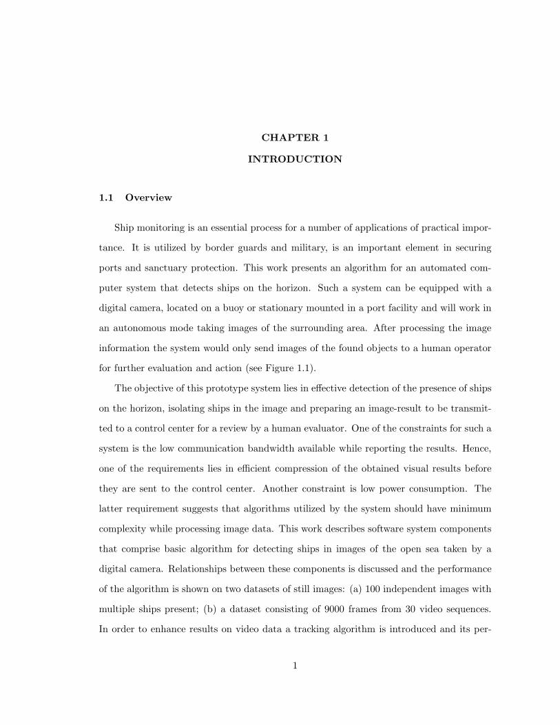
for further evaluation and action (see Figure 1.1).

The objective of this prototype system lies in effective detection of the presence of ships

on the horizon, isolating ships in the image and preparing an image-result to be transmit-

ted to a control center for a review by a human evaluator. One of the constraints for such a

system is the low communication bandwidth available while reporting the results. Hence,

one of the requirements lies in efficient compression of the obtained visual results before

they are sent to the control center. Another constraint is low power consumption. The

latter requirement suggests that algorithms utilized by the system should have minimum

complexity while processing image data. This work describes software system components

that comprise basic algorithm for detecting ships in images of the open sea taken by a

digital camera. Relationships between these components is discussed and the performance

of the algorithm is shown on two datasets of still images: (a) 100 independent images with

multiple ships present; (b) a dataset consisting of 9000 frames from 30 video sequences.

In order to enhance results on video data a tracking algorithm is introduced and its per-

1

Figure 1.1. Proposed buoy-based sea-traffic monitoring system.

formance is shown. In summary some improvements for more reliable and robust marine

vessel detection algorithm are suggested.

1.2 Previous Work

1.2.1 Marine Vehicles Detection

Most of the job in sea monitoring is done using radio radars [1]. They rely on reflection

of electromagnetic waves from a change in the dielectric or diamagnetic constants. A

radar transmitter emits radio waves, which are reflected by the target. Reflected radio

waves are detected by a radar receiver. Target objects are detected based on the latency

between transmitted and received signals. A range of objects, including weather formations,

ground and sea surfaces reflect radio waves and, thus, may be detected. However, the radio

reflection is particularly high for electrically conductive materials, such as metal and carbon

fiber, the material widely used for frames of the marine vessels and aircraft.

2

Radar’s ability to detect metal objects of various sizes depends on the choice of oper-

ating frequency. High (microwave) frequency marine radars are employed in most of the

current vessels, aircraft and ground stations for ships detection. They have properties of

reliable detection of even relatively small (with radar cross section of about 1 m2 objects.

However, the operating range of those radars is limited by linear distance to the target

objects and usually does not exceed 10-20 miles or more for airborne installed systems.

Another category of radars, ground wave over-the-horizon radars (GWOTHR), use

lower frequencies of radio waves, and thus, can propagate signal along the curved surface.

They also use the fact of refraction of radio waves in ionosphere. This provides GWOTHR

radars with surveillance capabilities over very large areas. For example [2] reports results

for technical capabilities of Northern Radar’s Cape Race Ground Wave Radar system

which had the potential to provide surveillance of over 160,000 square kilometers. Its

range of targets included ships, icebergs, as well as environmental parameters such as

surface currents and sea states. This category of radars is able to detect low-flying aircraft

on big distances but detection of marine vehicles on big distances is limited to due the

small radial Doppler velocity of the vessels: the targets’ Doppler usually shares the same

spectral region with the continuum of high order sea clutter [3].

Another approach to ship detection is described in [4]. This method uses magnetic fields

around magnetic targets to detect relatively large ships on the surface or even submarines

in a submerged state. A magnetometer onboard an aircraft measures anomalies in the

magnetic field in the area surrounding the aircraft. Although conceptually proven to detect

artificial metal objects, this exotic method, however, is more suitable for geology, for finding

deposits of iron ore or other metal resources. Detection of sea target is limited by the

distance from magnetometer to the target. The nature of magnetic field requires the

aircraft carrying the system to be in the close vicinity to the target.

The next category of radars, SAR (Synthetic Aperture Radar) has many applications

in remote sensing and mapping. The approach uses sophisticated postprocessing of radar

data to produce a very narrow effective microwave beam [5]. SAR can only be used

on moving platforms to conduct sensing over relatively immobile targets. The two most

3

used platforms for SAR are satellites (for spaceborne SAR) or aircraft (for airborne SAR).

Marine vehicles and coast line detection by SAR has become a topic of considerable interest

since the upsurge of demand for this kind of information in the commercial market. SAR

capabilities include all weather and all day detection, high resolution and wide coverage

(around 100x100 km). The result of sensing using the radar is an image of the ocean

surface. Current systems used for ship detection vary in the computer vision approaches

to detect the objects of interest. Many techniques [6], [7] search for features of the wake

of a ship in a SAR image. In [8] the Radon transform of SAR images of ship wakes and

ocean waves was computed and an enhancement operator within the transform space was

applied.

In more advanced work using SAR images instances of ships are assigned a class or

category (i.e. destroyer, aircraft carrier). In [9] radar images were used to classify ships

based on global features. Morphological analysis of the object boundary from SAR images

was utilized in [10]. Classification of the ships and their motion parameters is described

in [11] and [12].

Other imaging sensors were used for ship detection as well. Forward Looking Infra Red

(FLIR) cameras is often a good sensor of choice because the images they provide are insen-

sitive to lighting conditions. This imaging sensor is more desirable in military applications

because it does not reveal the location of the imaging system. Many approaches can be

found the in the literature for ship classification in FLIR images. In [13] they used the

principal component global features and similarity matching to classify ship silhouettes.

The authors of [14] used neural networks applied directly to image pixels. Recent work on

ship classification in [15] uses a k Nearest Neighbor classifier on shape features extracted

with MPEG-7 region-based shape descriptor.

A notable disadvantage of FLIR systems is the low resolution of the images obtained

which requires a relatively small viewing distance of the imaging system to the target.

It is also more power consuming and, thus, is less capable for autonomous operation.

The approach described in [16] uses solely computer vision algorithms and image data

from regular digital cameras (in the visual spectrum) to detect marine vehicles. It is

4

aimed for autonomous operation, under power and communication bandwidth constraints.

The applications for its use include local sea traffic monitoring in sanctuaries and port

zones. Images of open sea taken from a forward looking camera installed on a buoy. After

detecting horizon line the system looks for objects lying on it. The system is intended

to monitor only local traffic, within visible distance. However, the absence of radars and

reliance on simple computer vision algorithms makes the potential system cheap and easy

in deployment and maintenance. This document enhances preliminary results described

in [16]. It adds additional robustness to horizon detection for single images. It also uses

tracking techniques to improve detection in video sequences.

1.2.2 Horizon Detection

Another category of related work that should be mentioned includes horizon detection

in images. Accurate horizon detection gets considerable attention in this thesis. According

to the literature survey performed for this work most of horizon detection approaches

were designed for navigation of micro air vehicles (MAV). While larger aircraft may have

high-precision gyros to sense angular rates or acceleration, smaller MAV have very strict

constraints for payload capacity, dimensions, and electrical power. MAV autonomous flight

control system in many cases relies on cheap and light on-board imaging sensors such as

cameras, which, however, provide rich information content. In addition to surveillance

tasks that have been considered as the primary mission of MAV, such imaging sensors

allow estimation of navigation parameters. Pitch angle and roll angle of a MAV can be

extracted based on the horizon line in the video images. Several vision systems have been

reported to provide vision-based horizon-tracking.

One research group, very active in vision-based navigation, has published a number

of papers related to horizon detection [17, 18, 19, 20]. Their basic approach, a statistical

horizon detection algorithm, attempts to minimize the intra-class variance of the ground

and sky distribution. The horizon is considered a line with high likelihood of separating

the sky from ground (or non-sky) regions.

5

Other approaches developed by different authors [21, 22] rely on more simple and less

computationally intensive algorithms. The horizon angle is found as a function of the

average coordinates for sky and non-sky classes. The angle of the horizon is determined

by taking the perpendicular of the line joining sky and non-sky centroids. Sky and non-

sky regions are distinguished by a simple thresholding criterion based on the brightness of

pixels in a grayscale image.

A considerably different technique is described in [23]. It uses an idea similar to skew

detection in document image analysis, i.e. detecting the skew of the scanned documents.

The original image is preprocessed and edges are extracted. Projection profiles of edges in

the image for different angles are obtained and the horizon is found in the profile corre-

sponding to the largest peak of such a projection.

The approach described in [24] was designed not only for horizon detection but also to

avoid obstacles during MAV flights. The authors classify regions in the image into sky and

ground/obstacles and obtain boundaries of the safe area ahead of the aircraft as well as

angular parameters of the aircraft determined from the horizon line. Another classification

approach, not related directly the MAV navigation, is described in [25]. The horizon is

modeled as a line separating sky and non-sky pixel and is found after image content is

classified using numerous features into two classes - sky and non-sky.

Several other works related to MAV navigation report more integration with hardware,

often allowing on-board processing of the data. One research group developed horizon

detection equipment that is light enough to be airborne [26]. They use a thermal imaging

camera and scanned linear array. Similar approaches that use the infra-red spectrum are

used in aerospace application for stabilizing aircraft and are described in [27].

Chapter 5 will continue the discussion about horizon detection optimal needed for this

work. The mentioned horizon detection algorithms will be reviewed in more detail and

several will be evaluated for performance.

6

CHAPTER 2

BACKGROUND

2.1 Edge Detection

Edge detection is a research field within image processing and feature extraction and

there are many different approaches to it. The goal of edge detection is to mark the points

in an image at which the intensity changes sharply. Sharp changes in pixels intensity in an

image usually reflect important events and changes in world corresponding to the image.

Examples of edge detectors include Sobel, Laplace and Canny and other edge detectors

[28], [29], [30]. This work uses Canny edge detector [31].

The algorithm used in Canny’s method follows a list of criteria to improve edge detection

in comparison to other methods. Its advantages include low error rate, well-localized edge

points with minimum distance between the actual edge, and single edge response. The

algorithm consists of the following six steps:

• Noise in the original image is filtered out before locating and detecting any edges.

Because the Gaussian filter [28], [32] can be computed using a simple mask, it is

used exclusively in the Canny algorithm. Once a suitable mask has been calculated,

Gaussian smoothing is performed using standard convolution methods.

• The edge strength is found by taking the gradient of the image. 2-D spatial gradient

measurement is performed by convolving two (vertical, and horizontal) 3x3 kernels

around each pixel in the image. Then, the approximate absolute gradient magnitude

(edge strength) at each point can be found. The Sobel operator uses a pair of 3x3

convolution masks, one estimating the gradient in the X direction (columns) and the

other estimating the gradient in the Y direction (rows). The magnitude, or edge

7

strength, of the gradient is then approximated using the formula:

|G| = |Gx| + |Gy| (2.1)

• Edge direction is found from the gradient magnitude in the X and Y direction using

the following formula:

θ = arctan(Gx

Gy) (2.2)

• The non-maximum suppression, used to trace along the edge in the edge direction, is

applied after the edge directions are known. This results in a thin line in the output

image.

• Hysteresis is used as a means of eliminating streaking. Streaking is the breaking up

of an edge contour caused by the operator output fluctuating above and below the

threshold. If a single threshold, T1 is applied to an image, and an edge has an average

strength equal to T1, then due to noise, there will be instances where the edge dips

below the threshold. Equally it will also extend above the threshold making an edge

look like a dashed line. To avoid this, hysteresis uses two thresholds, high (T1) and

low (T2). Any pixel in the image that has a value greater than T1 is presumed to

be an edge pixel, and is marked as such immediately. Then, any pixels that are

connected to this edge pixel and that have a value greater than T2 are also selected

as edge pixels.

2.2 Connected Components Algorithm

Extracting and labeling of various disjoint and connected components in an image is

an important postprocessing step of ship detection. The connected components labeling

algorithm [33] is applied on a binary image to group its pixels into components based on

pixel connectivity, i.e., all pixels in a connected component share similar pixel intensity

values (zero or one) and are in some way connected with each other. Once all groups

8

have been determined, each pixel is labeled with a number according to the component it

was assigned to. The algorithm works by scanning an image, pixel-by-pixel (from top to

bottom and left to right) in order to identify regions of adjacent pixels which share the

same set of intensity values V .

Connected component labeling works on binary images and two different measures of

connectivity are possible: 4-connectivity and 8-connectivity, depending on the number

of neighbor pixel possible for connection. For the current project 8-connectivity is used,

however, for the purpose of simplicity only 4-connectivity is described here. The labeling

operator scans the image by moving along a row until it comes to a point p, where p denotes

the pixel to be labeled at any stage in the scanning process for which V = 1. When this

is true, it examines the four neighbors of p which have already been encountered in the

scan (i.e. the neighbors (I) to the left of p, (II) above it, and (III and IV) the two upper

diagonal terms). Based on this information, the labeling of p occurs as follows:

• if all four neighbors are 0, assign a new label to p, else

• if only one neighbor has V = 1, assign its label to p, else

• if more than one of the neighbors have V = 1, assign one of the labels to p and make

a note of the equivalences.

The equivalent label pairs after completing the scan are sorted into equivalence classes

and a unique label is assigned to each class. As a final step, a second scan is made through

the image, during which each label is replaced by the label assigned to its equivalence

classes. For display, the labels might be different gray levels or colors.

2.3 Kalman Filter

The Kalman filter [34], [35] provides a recursive solution to the linear optimal filtering

problem. Its domain of its applications includes stationary and non-stationary environ-

ments. The solution is recursive; each updated estimate of the state is computed from the

previous estimate and the new input data. The Kalman filter needs to store only the pre-

9

vious estimate, eliminating the need for storing the entire past observed data, and, thus is

computationally more efficient than computing the estimate from the entire past observed

data at each step of the filtering process.

The block diagram shown in Figure 2.1 describes a linear, discrete-time dynamic system.

The state vector, denoted by xk, is defined as the minimal set of data that uniquely

describes the unforced dynamical behavior of the system; the subscript k denotes discrete

time. The state vector is the least amount of data on the past behavior of the system

that is sufficient to predict its future behavior. On general, the state xk is unknown. To

estimate it, a set of observed data, denoted by the vector yk, is used. Process noise wk and

measurement noise vk, shown in the diagram, are represented by covariance matrices Q

and R, and are considered constant. The following set of equations describes the dynamic

system mathematically:

• Process equation

xk+1 = Fk+1,kxk + wk (2.3)

where Fk+1,k is the transition matrix, which relates the state xk from time k to time

k + 1 in the absence of noise. The process noise wk is assumed to be additive, white,

with normal probability. Its probability distribution has zero mean with a covariance

matrix defined by

E[wnwkT ] =

Qk for n = k

0 for n 6= k

(2.4)

where T denotes matrix transposition. The dimension of the state space is denoted

by m.

• Measurement equation

yk = Hkxk + vk (2.5)

10

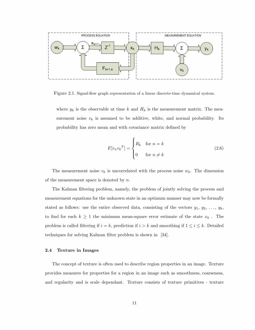
Figure 2.1. Signal-flow graph representation of a linear discrete-time dynamical system.

where yk is the observable at time k and Hk is the measurement matrix. The mea-

surement noise vk is assumed to be additive, white, and normal probability. Its

probability has zero mean and with covariance matrix defined by

E[vnvkT ] =

Rk for n = k

0 for n 6= k

(2.6)

The measurement noise vk is uncorrelated with the process noise wk. The dimension

of the measurement space is denoted by n.

The Kalman filtering problem, namely, the problem of jointly solving the process and

measurement equations for the unknown state in an optimum manner may now be formally

stated as follows: use the entire observed data, consisting of the vectors y1, y2, . . . , yk,

to find for each k ≥ 1 the minimum mean-square error estimate of the state xk . The

problem is called filtering if i = k, prediction if i > k and smoothing if 1 ≤ i ≤ k. Detailed

techniques for solving Kalman filter problem is shown in [34].

2.4 Texture in Images

The concept of texture is often used to describe region properties in an image. Texture

provides measures for properties for a region in an image such as smoothness, coarseness,

and regularity and is scale dependant. Texture consists of texture primitives - texture

11

elements. The three most used approaches to describe the texture of a region in an image

are statistical, structural and spectral. Statistical approaches show characterizations of

textures as smooth, coarse, grainy, and so on. Structural techniques deal with the arrange-

ment of texture elements, such as the description of texture based on regularity spaced

parallel lines. Spectral techniques are based on properties of the Fourier spectrum and are

used primarily to detect global periodicity in an image by identifying high energy or peaks

in the spectrum.

Because of their simplicity in describing texture this project uses statistical approaches.

Those include statistical moments of the gray level histogram, uniformity and entropy

calculated for a small region in an image. Let z be a random variable denoting gray levels

and let p(zi), i = 0, 1, 2, . . . , L− 1, be the corresponding histogram, where L is the number

of distinct gray levels. The nth moment of z, about the mean is

µn(z) =

L−1∑

i=0

(zi − m)np(zi) (2.7)

where m is the mean value of z (the average gray level):

m =

L−1∑

i=0

zip(zi) (2.8)

The second moment σ2(z) is a measure of gray level contrast that can be used to establish

descriptors of relative smoothness. For example, the measure

R = 1 −1

1 + σ2(z)(2.9)

is 0 for areas of constant intensity (the variance is zero there) and approaches 1 for large

values of σ2(z). Because variance values tend to be large for grayscale images with values,

it is normalized to the interval [0,1] for use in (2.9). This is done by simply dividing σ2(z)

by (L − 1)2 in (2.9). The standard deviation, σ(z), also is used frequently as a measure of

texture because values of the standard deviation tend to be more intuitive to many people.

12

The third moment,

µ3(z) =L−1∑

i=0

(zi − m)3p(zi) (2.10)

is related to the skewness of the histogram while the fourth moment is a measure of its

relative flatness. The fifth and higher moments are not so easily related to histogram shape,

but they do provide further quantitative discrimination of texture content.

Some useful measures based on histograms include a measure of uniformity given by

U =

L−1∑

i=0

P 2(zi), (2.11)

and an average entropy measure, which is defined as

e = −

L−1∑

i=0

p(zi) log2 p(zi) (2.12)

Because the probabilities have values in the range [0,1] and their sum equals 1, the

measure U is maximum for an image in which all gray levels are equal (maximally uniform),

and decreases from there. Entropy is a measure of variability and is 0 for a constant image.

In general coarse textures are built from larger primitives (texture elements), fine tex-

tures have smaller primitives. Coarse textures are characterized by lower spatial frequen-

cies, fine texture by higher spatial frequencies.

Figure 2.2 illustrates different texture measures. For each of the texture measures a

texture image of the resolution 256x192 has been received. The method of getting these

texture images is the following:

• Obtain a patch of an original image with the size of 11x11 around each pixel in the

grayscale image obtained from the original color image.

• Calculate a texture measure for this patch according to (2.7)-(2.12).

• Assign the result of the texture measure as a value of the pixel in the texture image.

13

• Normalize all values in the texture image equally in the range between 0 and 255.

Thus, for a grayscale image obtained from an original image there are six texture images.

14

Figure 2.2. Texture images. (a) original color image; (b) corresponding grayscale image of thered channel; (c) texture image using mean measure; (d) texture image using standard deviationmeasure; (e) texture image using smoothness measure; (f) texture image using third moment

measure; (g) texture image using uniformity measure; (h) texture image using entropy measure.

15

CHAPTER 3

ALGORITHMS

3.1 Overview

The literature section of this document described various methods for detection ma-

rine vehicles. These methods differ in technological approaches and potential capabilities.

However, most of them are similar in one important aspect: most of these methods are

characterized by the high cost of the equipment and maintenance. This creates a very

narrow category of users for such systems. In addition, rapid deployment of such systems

for monitoring purposes of local areas is difficult, it may require a radar installation or

access to satellite data.

This work focuses on detection of marine vehicles using imaging sensor such as digital

cameras or camcorders. The scope of surface area for monitoring is limited by visual

distance from some point in the ocean or shore. This may be be appropriate for some tasks

such as port security or sanctuary protection. In essence, the limitation and effectiveness of

the approach are similar to periscope of a submarine: marine vehicles are visually located

in image data obtained from a camera sticking out of the water surface. An ocean buoy

is considered a primary platform for such a system. An example of appropriate platform

can be shown on BSOP - the Bottom Stationing Ocean Profiler [36]. It is an autonomous

bouy-platform designed to carry a sensor payload, collect oceanic data and store or/and

transmit the data through a bi-directional RF satellite link to a control center. If equipped

with a proposed vision unit such a system could perform visual surveillance for passing sea

traffic.

The following sections enhance the previous work on algorithmic solution [16] for such

a system. In addition to detection of marine vehicles in single images (Section 3.2) other

16

settings are explored. Section 3.3 adds robustness to the detection approach for video data.

Such important aspects as detection, filtering, and tracking are also described.

3.2 Detection of Marine Vehicles in Single Images

Image segmentation and object detection is a broad topic of research in computer vision.

Usually, a particular application requires certain assumptions about the environment and

targets for detection. Approaches such as background subtraction or appearance similarity

are not appropriate for detection of marine vehicles in images with highly dynamic ocean

surface. Our assumption for the problem of marine vehicles detection is a relative position

between the sought marine objects and the ocean horizon line. That assumption is valid

for the case when images or video taken from the camera with image axis parallel to the

ocean surface and when the target marine vehicles are located within visual distance. Such

assumptions greatly facilitate localization of marine vehicles or other floating objects in

image data. This is because the ocean surface part of the image is rich in information

content and is difficult to process in terms of image analysis. On the other hand the sky

background, in front of which the sought marine vehicles are expected to be located, is

relatively homogeneous in color and has little texture, and thus, is easy to process.

Figure 3.1 shows the basic structure and order of steps in the algorithm to detect

marine vehicles in single images. The algorithm consists of six steps. During the image

acquisition step image data is obtained. Some preprocessing such as basic noise removal

is also done during that step. Preprocessed image is fed into two components - edge

detector and horizon detector, to obtain, correspondingly, edges from the original image

and the parameters of the horizon line. The postprocessing step of the algorithm combines

results from edge and horizon detectors and processes only edges that are located above

the horizon line. The connected components block of the algorithm provides the location

of the bounding boxes around the found marine vehicles. The output result consists of a

region from the original image inside the bounding box around found objects. Figure 3.2

shows a sequence of steps in ships detection on a sample image.

17

Figure 3.1. Basic structure of ship detection algorithm.

Detailed implementation of the algorithm is described in Subsections 3.2.1–3.2.4.

3.2.1 Image Acquisition

The image acquisition step uses a digital camera installed on a buoy to acquire images

of the surrounding area. The image data from the camera is provided in RGB format.The

focus of the camera is set to infinity and thus, captures only far-lying objects which are

expected to be above the horizon line. The driving factors of such an assumption are

the following: at long distances the line between camera and object of interest (a ship)

becomes parallel to the sea level and therefore all objects of interest have to exist above

the horizon. The height above the water on which the camera is mounted is a matter of

consideration. The effective range of detection is bigger when camera is mounted higher.

However, a closely located ship may not be exactly above the horizon line detected from

such a camera. For some settings the height of camera installation is also a matter of what

is practical. For example, buoy systems may not have a mast tall enough to install the

camera on the required height. In context of this work the dependency between the height

of installation and detection range of the system is not explored. Ideas about the optimal

height of the camera-mast for a possible ship surveillance system may be taken from the

design of submarine periscope systems [37].

18

Figure 3.2. Intermediate results during ship detection. (a) Original image. (b) Detected horizonline. (c) Edge-image. (d) Edges taken for consideration (above horizon line). (e) Result of

postprocessing step. (f) Bounding box over detected ship.

3.2.2 Edge Detection

The output of this step is a binary map of edges found in the original image. Edges

in the images reflect the regions in the images where pixel intensity changes quickly. For

a possible marine vehicle with distinct appearance it means sharp changes in intensity at

least around the contour of the target in front of sky background. Chapter 2 described the

Canny edge detector that was chosen for this work. Good edges should include the contour

of a marine vehicles: an edge map that creates a convex hull around the object and exclude

edges not belonging to the object. Edges also need to be consistent, possibly having as

few broken lines belonging to the same object as possible. The Canny edge detector has

three parameters: sigma (0.5-5.0), low (0.0-1.0) and high (0.0-1.0). Automatic search for

optimal parameters was not considered in the context of this work because of the difficulties

in creating precise pixelwise groundtruth. Manual search for parameters of the Canny edge

detector was conducted on a separate dataset of 27 images. The parameters were adjusted

to capture only well-defined long edges that are common for vessels with extensive contour

19

lines like yachts or barges. Figure 3.2 (c) shows an example of edge map detected for

original image in Figure 3.2 (a).

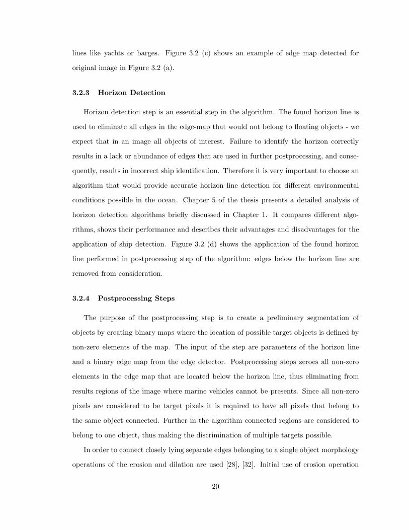
3.2.3 Horizon Detection

Horizon detection step is an essential step in the algorithm. The found horizon line is

used to eliminate all edges in the edge-map that would not belong to floating objects - we

expect that in an image all objects of interest. Failure to identify the horizon correctly

results in a lack or abundance of edges that are used in further postprocessing, and conse-

quently, results in incorrect ship identification. Therefore it is very important to choose an

algorithm that would provide accurate horizon line detection for different environmental

conditions possible in the ocean. Chapter 5 of the thesis presents a detailed analysis of

horizon detection algorithms briefly discussed in Chapter 1. It compares different algo-

rithms, shows their performance and describes their advantages and disadvantages for the

application of ship detection. Figure 3.2 (d) shows the application of the found horizon

line performed in postprocessing step of the algorithm: edges below the horizon line are

removed from consideration.

3.2.4 Postprocessing Steps

The purpose of the postprocessing step is to create a preliminary segmentation of

objects by creating binary maps where the location of possible target objects is defined by

non-zero elements of the map. The input of the step are parameters of the horizon line

and a binary edge map from the edge detector. Postprocessing steps zeroes all non-zero

elements in the edge map that are located below the horizon line, thus eliminating from

results regions of the image where marine vehicles cannot be presents. Since all non-zero

pixels are considered to be target pixels it is required to have all pixels that belong to

the same object connected. Further in the algorithm connected regions are considered to

belong to one object, thus making the discrimination of multiple targets possible.

In order to connect closely lying separate edges belonging to a single object morphology

operations of the erosion and dilation are used [28], [32]. Initial use of erosion operation

20

allows filtering out some small edges that do not belong to target object: parts of uneven

horizon line, different objects essential to the ocean environment - flying birds, clouds etc.

Further use of erosion and dilation with a bigger structural element allows connection of

binary regions that lie within a certain distance relative to the size structural element. The

size and shape of the structural element for this work were determined empirically on a test

dataset of 27 images. The disk shape was chosen for the structural element. The diameter

of the disk was equal to 2 pixels for filtering operations followed by disk with diameter 7

to connect closely lying pixel regions.

3.2.5 Labeling Components and Output

The connected components algorithm (described in Chapter 2) is used to detect bound-

ing boxes around the found objects and groundtruth objects (when performance is evalu-

ated), to find out the size of the objects and to filter out some of the segmentation results.

Every non-zero pixel from the output of the postprocessing step is assigned a label

by the connected components algorithm. Pixels that have the same label are connected

and belong to one detected object. Thus, this step transforms pixelwise representation of

the target to labelwise. By having the pixels of the objects labeled it is possible to check

the location of the furthest points of the object in the top, bottom, right, and left sides.

Locations of those pixels constitutes the position of the sides the bounding box around

the found object. Objects that have intersecting bounding boxes are merged by assigning

a single label to the pixels comprising them. After the merge step bounding boxes are

computed again and their size is calculated.

All found objects are checked for the proximity to the horizon. Only regions within 10

pixels of the horizon line are further considered to be targets. This operation reduces false

alarms caused by birds, clouds, and aircraft which are also located above the horizon line.

In the experiment objects which had size less then 6 pixels were eliminated from output.

That is justified by the fact that ships in the sea with such small size are less important for

a human evaluator and are usually located far enough from the place of interest. Filtering

of the small floating objects further reduces false alarm rate when the small regions above

21

the horizon line represent parts of uneven horizon in the sea, birds on the water surface,

etc.

The algorithm outputs the parts of the original image corresponding to the found

bounding boxes in connected components step (see Figure 3.2 (f)). Accuracy of detec-

tion of marine vehicles is described based on how well the found bounding boxes match

groundtruth boxes. Evaluation and performance metrics for such detection are shown in

Chapter 4.

3.3 Detection of Marine Vehicles in Video

Such heuristics as vicinity to the horizon line or segmentation techniques greatly reduce

the alarm rate and increase the overall accuracy of detection. Still, some steps of the

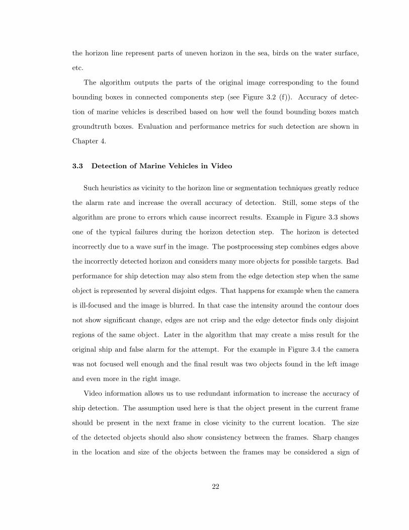
algorithm are prone to errors which cause incorrect results. Example in Figure 3.3 shows

one of the typical failures during the horizon detection step. The horizon is detected

incorrectly due to a wave surf in the image. The postprocessing step combines edges above

the incorrectly detected horizon and considers many more objects for possible targets. Bad

performance for ship detection may also stem from the edge detection step when the same

object is represented by several disjoint edges. That happens for example when the camera

is ill-focused and the image is blurred. In that case the intensity around the contour does

not show significant change, edges are not crisp and the edge detector finds only disjoint

regions of the same object. Later in the algorithm that may create a miss result for the

original ship and false alarm for the attempt. For the example in Figure 3.4 the camera

was not focused well enough and the final result was two objects found in the left image

and even more in the right image.

Video information allows us to use redundant information to increase the accuracy of

ship detection. The assumption used here is that the object present in the current frame

should be present in the next frame in close vicinity to the current location. The size

of the detected objects should also show consistency between the frames. Sharp changes

in the location and size of the objects between the frames may be considered a sign of

22

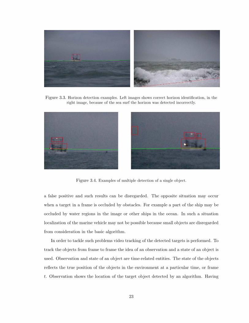
Figure 3.3. Horizon detection examples. Left images shows correct horizon identification, in theright image, because of the sea surf the horizon was detected incorrectly.

Figure 3.4. Examples of multiple detection of a single object.

a false positive and such results can be disregarded. The opposite situation may occur

when a target in a frame is occluded by obstacles. For example a part of the ship may be

occluded by water regions in the image or other ships in the ocean. In such a situation

localization of the marine vehicle may not be possible because small objects are disregarded

from consideration in the basic algorithm.

In order to tackle such problems video tracking of the detected targets is performed. To

track the objects from frame to frame the idea of an observation and a state of an object is

used. Observation and state of an object are time-related entities. The state of the objects

reflects the true position of the objects in the environment at a particular time, or frame

t. Observation shows the location of the target object detected by an algorithm. Having

23

several consecutive observations it is possible to decide the following about the state of the

object: its location and behavior. It is also possible to predict the next state of the object

based on a history of observations. Tracking of the object is considered successful when the

prediction matches the actual measurement, i.e. when based on the history of observations

of the object a prediction about the possible next location is made and confirmed by the

real detection of the object in that location in the next frame. In relation to marine vehicle

tracking it means, for example, that based on a 10 frame sequence the location of the

marine vehicle is predicted for the 11th frame. If later, in the 11th frame, a detection

algorithm shows the location of the marine vehicle that predicted location then the object

is tracked successfully.

Tracking allows handling situations with false alarms and missed detections. If the

history of object behavior does not support the measurement of its location, then such

detection of an object in the current frame can be disregarded. This reduces the false alarm

rate caused by the possible presence of noise in images. On the other hand, detection of an

object can be considered for a certain location in a frame in the video even if the detection

algorithm does not show presence of the object. That may happen when the history of the

object from the previous and following frames shows consistent behavior.

The Kalman filter, described in Chapter 2, is a good framework to implement vision

tracking of objects in video. The next subsection shows details of a filter implementation.

3.3.1 Use of the Kalman Filter

For this work two different filters are defined to track the following two entities: the

position of the center of the bounding box (centroid) and the bounding box dimensions.

Each of these two filters tracks the behavior of the two variables. Two auxiliary variables

for each filter describe the speed of change the main variables. For example for the first

filter the pair of variables that describe the position of the centroid - namely the x and y

coordinates are supplemented by auxiliary variables that describe the speed of movement of

this centroid along the x and y axes; horizontal and vertical dimensions of the bounding box

24

W and H are supplemented with the speed of changing of these variables in the horizontal

and vertical directions.

Equations (3.1)–(3.2) show the implementation of the Kalman filter for visual tracking

used in the thesis. The transformation matrix in (3.1) establishes the relation between

the main and auxiliary variables in the current and next frames. That relation reflects

the linear nature of the motion of the modeled object: the predicted value of the main

variable (such as location of the corner) in the next state k + 1 is different from the

previous state k on the amount of value of the corresponding auxiliary variable ∆xk:

xk+1 = xk + ∆xk. The measurement matrix in (3.2) shows correspondence between the

state vector and measurement vector. Other important variables used in the model are

state wk and measurement vk noises which are described by a normal distribution.

xk+1

yk+1

∆xk+1

∆yk+1

=

∣

∣

∣

∣

∣

∣

∣

∣

∣

∣

∣

∣

∣

1 0 1 0

0 1 0 1

0 0 1 0

0 0 0 1

∣

∣

∣

∣

∣

∣

∣

∣

∣

∣

∣

∣

∣

xk

yk

∆xk

∆yk

+ wk (3.1)

xmk

ymk

=

∣

∣

∣

∣

∣

∣

∣

1 0 0 0

0 1 0 0

∣

∣

∣

∣

∣

∣

∣

xk

yk

∆xk

∆yk

+ vk (3.2)

Here x and y represent the main variables such as the position of the center or dimension

of the bounding box. ∆x and ∆y are auxiliary variables.

The Kalman filter can tolerate big discrepancies, so called outliers in measurement or,

as it is often called in computer vision, small occlusions. In the case that a tracking object

is not found in a certain neighborhood of the predicted state it is considered that the object

is hidden and will not use the measurement correction but instead only prediction.

25

Figure 3.5. Outline of marine vehicle tracking algorithm. (a) Detection of marine vehicles insingle image or frame. (b) Tracking of detected objects through video sequence.

3.3.2 Tracking of Marine Vehicles

Our algorithm for object tracking is similar to the Multiple Hypothesis Tracking (MHT)

algorithm [38][39], but with significant modifications. The features of the algorithm in-

clude track initiation, continuation, and termination for multiple objects. Modifications

introduced for the purpose of this work are related to the resolution of data association

uncertainty as well as computational speedup.

Figure 3.5 shows the outline of the algorithm for tracking detected objects. The al-

gorithm starts the iteration for the current frame by analyzing history of the previously

tracked objects. It predicts the possible location and size of bounding boxes around objects

by using a linear Kalman filter as described above. Independently the current frame is a

subject of target detection by using the algorithm described in Section 3.2. Parameters of

detected objects are compared with predictions. Those tracks that had their object found

in the vicinity of the predicted location are updated to reflect the detection in the current

frame. Tracks that did not receive evidence of the object in the current frame use the

predictions instead of detections to avoid possible occlusions in the image. New tracks are

initiated for objects that enter the frame or in the beginning of the video sequence. Tracks

are terminated when objects leave the frame and also when tracks are not long enough.

Objects are considered to be marine vehicles if they have substantial tracking history.

26

Association between the detected objects and tracks is considered a one-to-one mapping.

The closest object in terms of euclidian distance is assigned to the track if it within the

validation region for that track.

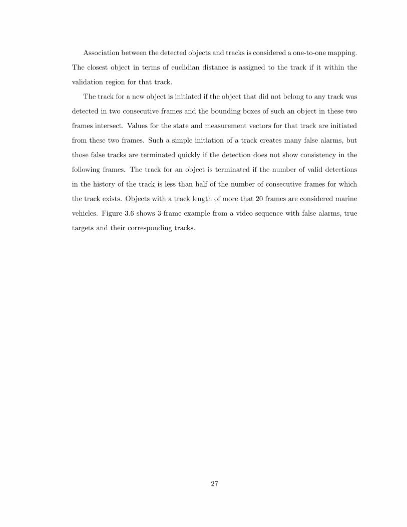
The track for a new object is initiated if the object that did not belong to any track was

detected in two consecutive frames and the bounding boxes of such an object in these two

frames intersect. Values for the state and measurement vectors for that track are initiated

from these two frames. Such a simple initiation of a track creates many false alarms, but

those false tracks are terminated quickly if the detection does not show consistency in the

following frames. The track for an object is terminated if the number of valid detections

in the history of the track is less than half of the number of consecutive frames for which

the track exists. Objects with a track length of more that 20 frames are considered marine

vehicles. Figure 3.6 shows 3-frame example from a video sequence with false alarms, true

targets and their corresponding tracks.

27

Figure 3.6. Example of tracking marine vehicles in video sequence. Sea waves are the main causeof false positives in basic detection algorithm. They are filtered out if the detections do not show

consistency in between the frames.

28

CHAPTER 4

DATA AND PERFORMANCE EVALUATION

4.1 Overview

This chapter of the thesis describes quantitative measures to evaluate the results of

marine vehicle detection and datasets used to evaluate the algorithms. One of the issues

with the evaluation of ship detection performance in general is that it is often a subjective

task: it is hard to say with 100% confidence if detection of an ship was carried out or not.

Therefore methods for evaluation of performance are a very important part of any such

system and should be defined in order to determine the success or failure of an algorithm,

measure improvements, or produce a useful description of the results.

The accuracy of detection of marine vehicles in this thesis is measured by comparing

output of the algorithm, or the candidate data, with the groundtruth, or target data.

Groundtruth is a set of results which are created by a human. For this work groundtruth

annotations were created by the researchers for both horizon and marine vehicles data in

order to evaluation performance of algorithms for both categories.

Quantitative comparison for different detection algorithms is possible by using mech-

anism of metrics. Metrics provide a description of how well the candidate data matches

the target data in a particular setting. Different metrics provide different aspects of per-

formance of algorithms and each metric usually has its advantages and disadvantages. In

content of this work metrics for both, horizon detection, and for the final result, marine

vehicle detection, are defined for a single image and for a set of images.

29

4.2 Metrics for Horizon Detection Evaluation

The horizon is modeled as a single straight line with zero pixel thickness that separates

two, assumably homogeneous, disjoint regions of pixels in the image - sky and ocean surface.

Every line is characterized by its two parameters in polar coordinates: ρ distance to the

origin of the coordinate system and Θ angle between the normal to the horizon line and the

vertical axis (see Figure 4.1 (a)). Given such a representation of the horizon it is difficult

to quantitatively compare lines in the target and candidate data just by the matching

corresponding parameters. In order to answer the question of how close two description

of horizon line are it was chosen to use pixelwise comparison of the candidate and target

data. The groundtruth image for horizon detection consists of black and white pixels which

are separated by envisioned horizon line. White pixels in such an image correspond to sky

regions of the image and black pixels denote the ocean surface. Figure 4.1 (b) shows an

example of such groundtruth.

Two metrics were chosen to reflect the accuracy of the horizon line detection. First

accuracy performance metrics represents the percentage of pixels in the image (throughout

the whole dataset) correctly separated into ocean surface and non-ocean surface regions by

the found line:

A1 =1

k

k∑

i=1

N ic

Ni

(4.1)

where k is the number of images in the dataset, N ic - number of pixels correctly separated

by the found horizon line in image i, Ni - number of pixels in the image i. This metric

provides a reference to a general performance of an algorithm on a dataset of images. Its

main disadvantage is that bad visual performance of horizon detection on some images may

stay unnoticed by the such metric output if the majority of other images in the dataset are

processed well.

Second metrics is aimed to reflect performance of the algorithm on each of the image

of the dataset. The horizon line in an image is considered to be detected correctly if the

30

Figure 4.1. Horizon representation. (a) The horizon is represented as a straight line in polarcoordinates with parameters ρ and Θ. (b) Groundtruth for an image. The white color regions

corresponds to the sky (above the horizon), black regions correspond to the ocean surface.

percentage of pixels in the image correctly separated by the horizon line is above a specified

threshold. The percentage of such images in the dataset will define the second accuracy

metric:

A2 =nc

k(4.2)

where k is the total number of images in the dataset and nc is the number of images in the

dataset where the horizon line was detected with accuracy above the given threshold:

N ic

Ni

≥ T (4.3)

where T is the threshold value.

Another important characteristic for which the horizon detection algorithms were eval-

uated was the running time of the algorithms. The main requirement for fast performance

may come from systems that do real time processing of video data or systems where the

number of CPU cycles used for detection is required to be at the minimal level in order

satisfy power consumption constraints.

31

4.3 Metrics for Marine Vehicle Detection Evaluation

Detection of marine vehicles is more complicated than horizon detection and thus, more

aspects need to be evaluated. In single images detection implies spatial localization of found

ships (allowing multiple vessels per image). In video, combination of spatial and temporal

dimensions requires tracking the target from frame to frame, thus temporal localization of

the same objects throughout the frame sequence should be performed.

Marine vehicles considered for detection in images and video are, in most cases, compact

objects and therefore can be covered by simple bounding shapes. It was chosen to use

rectangular bounding box as a shape to mark the groundtruth and output data of the

algorithm. For simplicity of representation, the bounding box is always oriented so that its

sides are parallel to the axes of the image plane. Each groundtruth image is a binary image

where white regions correspond to background and black rectangular regions correspond

to the target objects.

Process of creating groundtruth for marine vehicles is tedious when the number of

groundtruth images is substantial. To facilitate creation of groundtruth the author used

software ViPER [40] to create bounding boxes around targets in the data. ViPER tool was

created to provide repeatability and comparability in performance evaluation. Attributes

of descriptors, such as bounding boxes, may be recorded for arbitrary sets of consecutive

frames in the video which makes such tool very convenient for the researcher.

Detection and tracking measures for performance evaluation were adopted from [41].

These comprehensive metrics account for important measures of system performance such

as number of objects detected and tracked missed objects, false positives, fragmentation

in both spatial and temporal dimensions, and localization error of detected objects. The

following notations are used to define the metrics:

• Gi denotes ith target object at the sequence level and G(t)i denotes the ith target

object in frame t.

• Di denotes ith candidate object at the sequence level and D(t)i denotes the ith detected

object in frame t.

32

• G(t) is the set of targets in a single image t

• D(t) is the set of candidates from the algorithm.

• NG and ND denote the number of unique targets and number of unique candidates

for the sequence of frames.

• Nframes denotes the number of frames in the sequence.

• Nmapped is the number of mapped target and candidate pairs.

Frame Detection Accuracy (FDA) is the metric that reflects accuracy of detection

localization. It calculates the overlap between the target and candidate objects as a ratio

of the spatial intersection between the two objects and the spatial union of them. The

sum of all of the overlaps is normalized over the average of the number of targets and

candidates. For a frame t with N(t)G targets and N

(t)D candidates FDA(t) is defined as

follows:

FDA(t) =OverlapRatio

[N

(t)G

+N(t)D

2 ]

(4.4)

where, OverlapRatio =

N(t)mapped∑

i=1

|G(t)i

⋂

D(t)i |

|G(t)i

⋃

D(t)i |

(4.5)

Sequence Frame Detection Accuracy metric shows the performance of detection for the

whole frame sequence. This metrics accounts for both missed detects and false positives

in one score. It is expressed as FDA calculated over all of the frames in sequence and

normalized to the number of frames in the sequence where targets or candidates existed:

SFDA =

∑t=Nframes

t=1 FDA(t)∑t=Nframes

t=1 ∃(N(t)G OR N

(t)D )

(4.6)

Next metrics are similar to the horizon metric (4.2). They take hard decision for

each target object: detected or not detected. A target object is considered detected if

minimum proportion of its area is covered by the candidate. Thresholded Overlap Ratio

33

and Thresholded Frame Detection Accuracy (FDA-T) are defined as follows:

ThresholdedOverlapRatio =FDA − T

|G(t)i

⋃

D(t)i |

(4.7)

where

FDA − T =

|G(t)i

⋃

D(t)i |, if

|G(t)i

⋂

D(t)i

|

|G(t)i

⋃

D(t)i

|≥ Threshold

|G(t)i

⋂

D(t)i |, if

|G(t)i

⋂

D(t)i

|

|G(t)i

⋃

D(t)i

|< Threshold & non − binary thresholding

0, if|G

(t)i

⋂

D(t)i

|

|G(t)i

⋃

D(t)i

|< Threshold & binarythresholding

(4.8)

The Sequence Track Detection Accuracy (STDA) is a measure of tracking performance

over all of the objects in the sequence and is calculated as following:

STDA =

Nmapped∑

i=1

∑Nframes

t=1 [|G

(t)i

⋂

D(t)i |

|G(t)i

⋃

D(t)i |

]

N(Gi

⋃

Di 6=0)(4.9)

The Average Tracking Accuracy (ATA) is defined as STDA per objects:

ATA =STDA

[NG+ND

2 ](4.10)

ATA is a spatio-temporal metric which penalizes fragmentations in the temporal and spatial

dimensions. It accounts for the number of objects detected and tracked, missed objects,

and false positives.

4.4 Datasets

The datasets discussed in this work were used to evaluate performance of detection of

two categories of entities: marine vehicles and the horizon. The final result of the work

is evaluation of detection of marine vehicles in single images and in video. The need to

evaluate horizon detection algorithms was due to high correlation between correct horizon

detection and good accuracy in detecting marine vehicles. Chapter 5 compares different

34

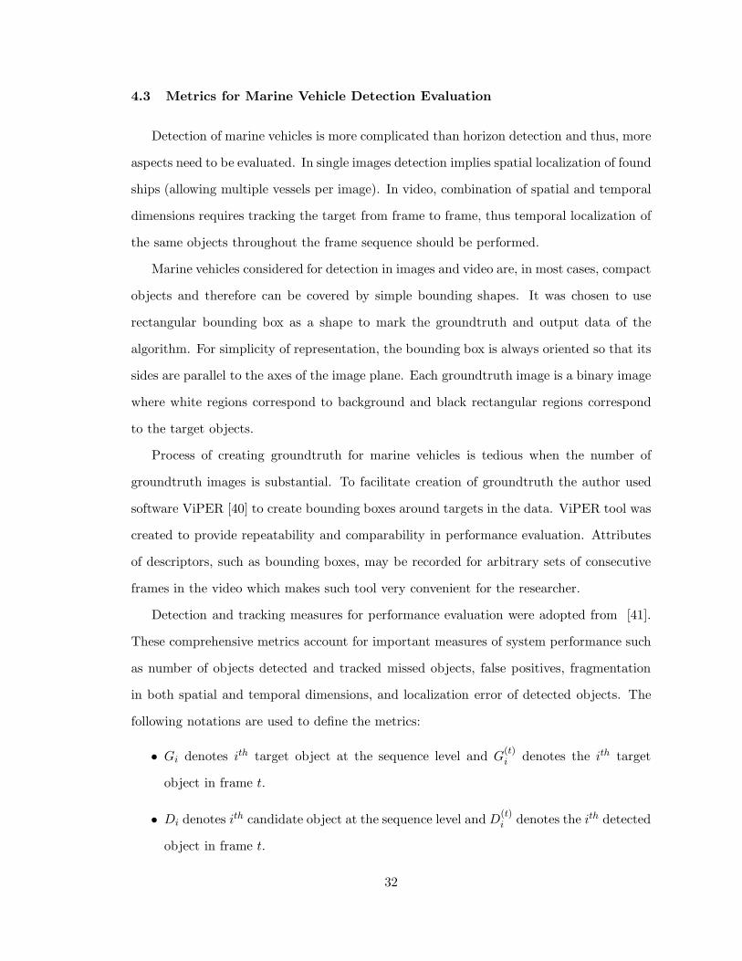
Figure 4.2. Examples of images from datasets used for testing horizon detection algorithms. (a)HORIZON DATASET 1 - no floating objects, clear horizon; (b) HORIZON DATASET 2 - marine

vehicles presents on the horizon line. Data of the same nature was used in SHIP DATASET 2

horizon detection algorithms in terms of accuracy of horizon detection on the two datasets

of images.

The first dataset, further referred as HORIZON DATASET 1, was chosen to test the

general characteristics of the horizon detection algorithm: ability to correctly detect horizon

line in images where only sea and sky region were present. This dataset consisted of 160

frames chosen randomly from video sequences taken by a camera installed on a buoy in the

open sea. A separate set of 10 similar frames was used for training purposes. All images

(frames of the video) were color images of resolution of 720x480.

The second dataset, referred to as the HORIZON DATASET 2, represented 150 frames

picked in a similar way from video sequences taken by the same buoy camera. Many of

these images contained ships, floating objects, or waves that made the horizon line look

uneven. Examples of images in both horizon datasets are shown in Figure 4.2.

Groundtruth for both sets was created as described in Section 4.2. For images where the

waves, ships, or other objects were present this groundtruth line represented the horizon

envisioned without any objects. This location of horizon line would provide the best cue

for further segmentation of the image in order to locate the sought marine vehicles.

For evaluation of performance of the marine vehicles detection algorithm datasets of

still images and video sequences were used. Hereafter, SHIP DATASET 1 refers to the

35

dataset of 100 images taken by a digital camera in daylight conditions. The camera was

installed onshore and the images contained only ocean surface, floating objects including

ships. The images did not contain any coastal objects. All images in the dataset were in

resolution of 1280x960. Figure 4.3 shows a sample image from this dataset.

The second dataset for marine vehicle evaluation, further referred to as SHIP DATASET

2, consisted of 30 video sequences. The video for the dataset was taken from a digital

camcorder mounted on a buoy in open ocean in daylight. The content of the video is the

ocean surface with possible single ship present and no coastal objects. The mentioned

marine vehicle in the video sequence could be present the whole time, could enter or

leave the frame at some point of time, or be absent throughout the video sequence. Each

video sequence was 10 seconds long and contained 300 frames (30fps) and was created

at a resolution of 720x480. The total number of frames in the dataset is 9000. Original

video sequences from the camcorder were recorded in MPEG-1 format but the data for

the algorithm were fed frame by frame. An important aspect of the SHIP DATASET 2 is

the fact that, although, the nature of the data is sequential, the algorithms were tested to

detect marine vehicles in both settings. In the first setting the frames of the videos were

considered independently from neighboring frames to test detection of the basic algorithm

as in single images. In the second setting considered tracking a marine vehicle from frame

to frame and, thus, was working on these frames as with ordered sequence.

Images for horizon detection datasets were of the same nature as SHIP DATASET 2,

so Figure 4.2 can serve for illustration purposes of data in SHIP DATASET 2 as well.

Groundtruth for the both ship datasets was created as described in Section 4.3. Chapter 6

discusses results for detection of marine vehicles.

36

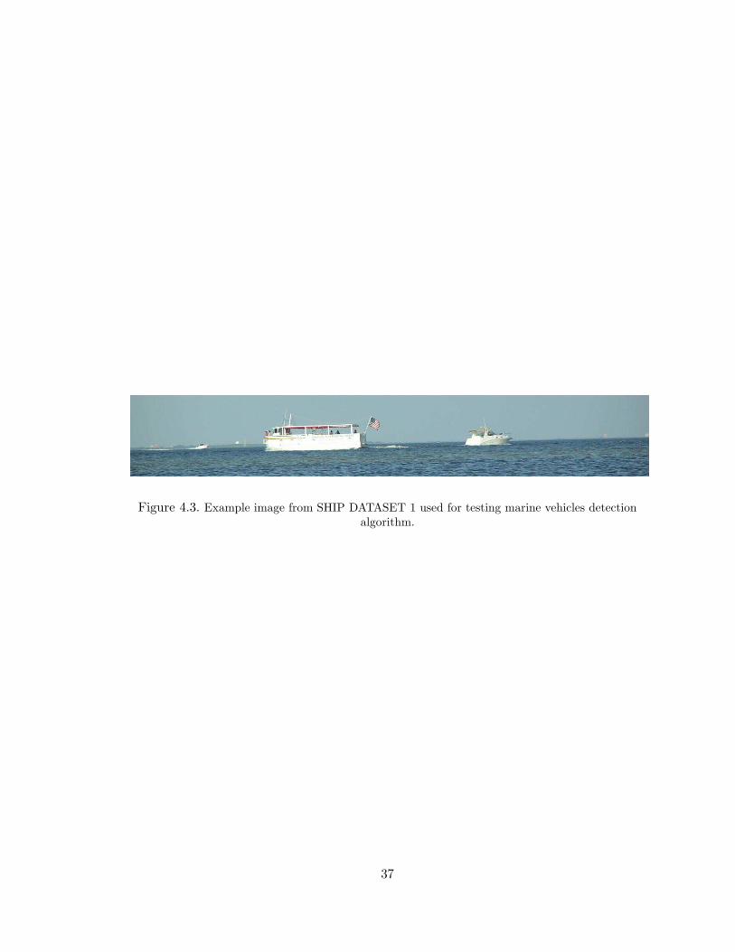
Figure 4.3. Example image from SHIP DATASET 1 used for testing marine vehicles detectionalgorithm.

37

CHAPTER 5

COMPARISON OF HORIZON DETECTION ALGORITHMS

5.1 Overview

Detection a ship in the vicinity of the horizon line is much easier and reliable than

trying to segment out a ship-blob out of the whole horizon image. Horizon detection is

more robust and its precise identification reduces the possible search space for marine

vehicles. Also segmentation of a ship out of the sky background can be performed with

simple image processing techniques compared to complex methods of object segmentation

out of the whole sky-sea image.

This chapter investigates the performance of the horizon detection algorithms described

in Chapter 1 on two different datasets of horizon images (see Section 4.4). The first set,

HORIZON DATASET 1, contains only horizon images of clear ocean surface without ma-

rine vehicles (see Figure 4.2 (a)). The second test set, HORIZON DATASET 2, introduces

ships and other floating objects on the horizon which generally influence horizon detection

(See Figure 4.2 (b). Some modifications to the original algorithms, introduced for the

purpose of better performance of ”ship images” were tested on the second dataset.

Particular re-implementations of horizon detection algorithms and their modification

will be named.

The horizon detection algorithms described in Chapter 1 were developed by teams of

researchers mostly for projects related to navigation of unmanned aerial vehicles (UAV).

Requirements for these algorithms were quite different from the requirements for the algo-

rithm described in this work. While navigation of UAV needs the horizon line in order to

avoid obstacles that are assumed to be below the horizon our application needs the horizon

line for reliable marine vehicle segmentation in images and video sequences which are as-

38

Figure 5.1. Example of failure of horizon detection. Assumption that the image consists of tworegions - sky and non-sky leads to the detection of horizon line above the vessel.

sumed to be located above the envisioned horizon line. Output of the algorithms that may

be suitable for navigation of UAV may not be appropriate for detection of marine vehicles.

Figure 5.1 shows the result of the horizon detection algorithm described in [18]. Because

of the vessel present in the image the algorithm found the line that best separates sky and

non-sky image lies above the sought ship, a result not acceptable for our application.

The literature review section of this document contains references to five categories of

approaches to detect horizon in images. Some of these approaches [26, 27] rely on specific

hardware to obtain images, and, thus, are not appropriate in the context of our algorithm.

The approach described in [21, 22] was designed to use the horizon as an estimator for roll

and pitch angle, and precision of the horizon line in the image itself was not the primary

target. The angle of the horizon is determined by taking the perpendicular of the line

joining sky and non-sky centroids. In case of rectangular images (source of our data),

the line between the centroids does not turn out exactly perpendicular to the horizon. In

addition the process of assigning labels to pixels into sky/non-sky classes based just on the

grayscale intensity value is in itself very inaccurate. An interesting and fast approach [23]

to apply a projection profile to an edge-image is good enough for straight horizon lines with

little texture (source of edges) coming from the ocean surface. But as it was tested with

some images from our evaluation dataset this may not be the case, and some anomalies in

horizon detection are observed even for simple images.

39

It was decided to concentrate on two main categories of approaches for horizon detec-

tion. The first category, described in a number of papers [17, 18, 19, 20], is a statistical

approach that tries to minimize intra-class variance between two categories of pixels. This

approach does not assume any training and is referred to as unsupervised. The second cat-

egory of algorithms, described in [24, 25], assumes training of a classifier on some labeled

data and is referred as supervised approach. The next two sections describe in detail these

original algorithms. The following sections show some modifications to these algorithms

during our re-implementation, as well as a comparison of performance of these algorithms.

5.2 Horizon Detection: Unsupervised Approach

The unsupervised approach [18] to horizon detection algorithm uses two basic assump-

tions:

• the horizon line appears in the image approximately as a straight line; and

• the horizon line separates the image into two regions that have different appearance

- sky and non-sky. In the sky region pixels will look more like other sky pixels, and

less like non-sky, and vice versa.

The first assumption reduces the search space for all possible horizons to a two-dimensional

search in line-parameter space. For each possible line in that two-dimensional space a spe-

cial criterion determines how well that particular line agrees with the second assumption

or in other words how well the correct horizon line separates the image into two regions

that have different appearance. The method utilizes the normal representation of a line

(see Figure 4.1 (a) for illustration):

x cos Θ + y sinΘ = ρ (5.1)

where (x, y) are the coordinates of the points on the line, Θ is the angle representing the

rotation of the line, and ρ is the perpendicular distance from the line to the origin.

40

The RGB color was chosen as a measure of appearance. For any given hypothesized

horizon line, the pixels above the line are labeled as sky, and pixels below the line are

labeled as non-sky. All hypothesized sky pixels are denoted as,

xis = [ri

sgisbi

s], i ∈ {1, . . . , ns} (5.2)

where ris denotes the value for intensity of the red channel in RGB, gi

s denotes the green

channel value and bis denotes the blue channel value of the i -th sky pixel. All the hypoth-

esized non-sky pixels are noted as,

xig = [ri

g, gig, bi

g], i ∈ {1, . . . , ns} (5.3)

Given these pixel groupings, the assumption that sky pixels look similar to other sky

pixels, and that non-sky pixels look similar to other non-sky pixels is quantified. One

measure of this is the degree of variance exhibited by each distribution. The proposed

optimization criterion for such variance is the following:

J(Θ, ρ) =1

Σs + Σg

(5.4)

based on the covariance matrices and of the two pixel distributions,

Σs =1

ns − 1

ns∑

i=1

(xis − µs)(xi

s − µs)T (5.5)

Σg =1

ng − 1

ng∑

i=1

(xig − µg)(xi

g − µg)T (5.6)

where ns is the number of sky-pixels, ng - number of non-sky pixels, and µs and µg are

mean vectors for color-intensity of the sky and non-sky pixel distributions and are defined

as

µs =1

ns

ns∑

i=1

xsi , µg =

1

ng

ng∑

i=1

xgi (5.7)

41

Assuming that the means of the actual sky and ground distributions are distinct, the line

that best separates the two regions should exhibit the lowest variance from the mean. If the

hypothesized horizon line is incorrect, some non-sky pixels will be mistakenly grouped with

sky pixels and vice versa. The incorrectly grouped pixels will lie farther from each mean,

consequently increasing the variance of the two distributions. The incorrectly grouped

pixels will skew each mean vector slightly, contributing further to increased variance in the

distributions.

5.3 Horizon Detection: Supervised Approach

The approaches described in [24] and [25] use machine learning techniques to classify

each pixel in the image into sky and non-sky class based on its color and texture of a

region around it. The classification of the image into sky and non-sky in [24] is performed

using a support vector machine (SVM) classifier [42] that assigns a category for each pixel

based on its color in the RGB color space, after smoothing the image with a Gaussian

filter to reduce the effects of noise. The approach described in [25] compares multiple

classifiers and uses multiple texture features along with the color of pixels. The authors of

the paper conclude that SVM performs better than other classifiers due to the fact that

SVM is inherently a binary classifier.

Although idea of pixel classification is similar in both approaches methods of finding

the actual horizon line from the classified image are different. In [24] the horizon is found

by searching for the line that best represents the boundary between binary sky segmented

image into sky and ground. The first step is to apply standard morphology operations of

erosion and dilation [28], [32] to the binary segmented image to remove any small sections of

misclassified pixels. The border between sky and ground regions is then found by smoothing

the binary image and classifying all pixels with values near 0.5 as boundary pixels. The

horizon line detection is performed using the Hough transform [28] on the border image

with a normal representation of a line. Each line in (X,Y ) space can be represented by a

point in (Θ, ρ) space. Conversely, each point in the (X,Y ) space represents a set of lines

42

in (Θ, ρ) space, which correspond to all of the possible lines that pass through that point.

Thus, for each point in (X,Y ) space, a vote is placed in each bin of a discretized (Θ, ρ)

space that corresponds to all possible lines that pass through that point. Bins in (Θ, ρ)

space that receive a large number of votes correspond to probable lines. The best horizon

is chosen as the candidate line which minimizes the cost function:

J(Θ, ρ) =∑

i,j

~e(~xij) (5.8)

~e(~xij) =

0 if f(~xij) = 1, (i, j) is above horizon

α if f(~xij) = −1, (i, j) is above horizon

1 if f(~xij) = 1, (i, j) is below horizon

0 if f(~xij) = −1, (i, j) is below horizon

(5.9)

where f(x) is the classification output, 1 for sky, -1 for ground, xij is the color vector from

the pixel at (i, j) in the image, and α is a positive constant. Thus, J(Θ, ρ) is a weighted

sum of all of the pixels above the candidate horizon classified as non-sky and all of the

pixels below the candidate horizon classified as sky.

The other method [25] in order to find horizon line in a classified image uses an

approach similar to the one described in Section 5.2. But instead of color information used

to describe each pixel, binary information (class of a pixel) is used.

5.4 Horizon Detection Performance on the Dataset without Ships

The algorithms that were tested on this dataset of images included the horizon detection

algorithm described in Section 5.2, a derivation of it that includes texture, and an algorithm

[24] described in Section 5.3. The algorithm [25] which uses classification of pixels in the

image into sea surface/non-sea surface based on many texture features was not considered

43

because of many computationally-intensive texture measurements needed to be performed,

operations that make the run-time prohibitively big.

The algorithm from [18], further called UNSUPERVISED, was implemented based on

the paper’s description as the search for the best parameters in two steps. During the

first step the algorithm used the image scaled to 1/5 of the original dimension in order

to find approximate parameters’ values. Scaling of the image is done for the purpose of

speeding up the computations. The second step searches for the horizon parameters in the

original image (without scaling) but uses the result of the first step as a starting point and

the search is performed in the limited vicinity of the search result of the first step, thus,

refining the result of the first step. Features used to distinguish sky and non-sky regions

are RGB intensity of the pixels that comprise them available directly from the input image.

A derivation of the UNSUPERVISED algorithm that uses texture information, further

called UNSUPERVISED-TEXTURE, uses the same two-step approach to find the horizon

parameters, but along with RGB colors it also incorporated texture measurement of uni-

formity (see (2.11) and Figure 2.2 (g) for illustration). Uniformity was chosen out of the

number of texture features described in Section 2.4 because it provides more distinction for

values in sea surface/non-sea surface regions. This texture measurement was assigned to

each pixel in the image and was calculated as a measurement of uniformity in the grayscale

patch of 10x10 pixels around the target pixels.

The last algorithm considered for evaluation [24], described in Section 5.3, is based on

classification of pixels into sea surface/non-sea surface. Further in the text this algorithm

is referred as SUPERVISED algorithm. To train the classifier 10 images of the training set

were used. The total of 1% pixels in each out of 10 training images was chosen randomly

to create a set of training vectors (about 38,000 vectors). The classification results were

followed by morphology operations of erosion and dilation with a structural element of disk

with radius equal to 7 pixels.

The Table 5.1 shows the performance results for the three algorithms obtained on the

HORIZON DATASET 1 with the metric described by (4.1). The results are shown for the

44

accuracy range of 82% and above, where the described horizon detection algorithm show

the biggest difference in performance.

Table 5.1. Accuracy of the horizon detection algorithms on the HORIZON DATASET 1according to metric (4.1).

UNSUPERVISED SUPERVISED UNSUPERVISED

TEXTURE

Accuracy of DetectionAccording to (4.1)

99.26% 98.89% 97.94%

Table 5.2 shows the performance of the same algorithms using the second metrics

described by (4.2). The chart in Figure 5.2 shows the same results visually.

Table 5.2. Accuracy of the horizon detection algorithms on the HORIZON DATASET 1according to metric (4.2).

THRESHOLD

Algorithm 84% 86% 88% 90% 92% 94% 96% 97% 98% 99%

UNSUPERVISED 98.75% 98.75% 98.75% 98.75% 98.75% 98.75% 98.75% 98.75% 97.50% 95.00%

SUPERVISED 98.75% 98.75% 98.12% 98.12% 96.88% 95.63% 95.00% 94.37% 92.50% 91.25%

UNSUPERVISED

TEXTURE

99.38% 99.38% 98.75% 97.50% 96.88% 93.13% 86.25% 76.88% 65.63% 46.88%

Table 5.3 shows running time in seconds per image for these algorithms. The algorithms

were implemented in MATLAB environment and tested on AMD Athlon 64 X2 Dual 3 GHz

processor. For the SUPERVISED algorithm the running time does not include training

time. Training of the algorithm is supposed to be done offline.

Table 5.3. Running time of the horizon detection algorithms on HORIZON DATASET 1 inrelative time units per image.

UNSUPERVISED SUPERVISED UNSUPERVISED

TEXTURE

Running time (time

units)

17.1 1.4 44.4

The result of comparison excludes the UNSUPERVISED TEXTURE algorithm from

further consideration because of its inferior accuracy and significant running time.

45

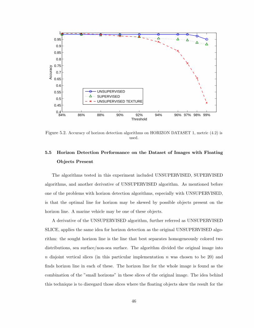
84% 86% 88% 90% 92% 94% 96% 97% 98% 99%0.4

0.45

0.5

0.55

0.6

0.65

0.7

0.75

0.8

0.85

0.9

0.95

1

Threshold

Acc

urac

y

UNSUPERVISEDSUPERVISEDUNSUPERVISED TEXTURE

Figure 5.2. Accuracy of horizon detection algorithms on HORIZON DATASET 1, metric (4.2) isused.

5.5 Horizon Detection Performance on the Dataset of Images with Floating

Objects Present

The algorithms tested in this experiment included UNSUPERVISED, SUPERVISED

algorithms, and another derivative of UNSUPERVISED algorithm. As mentioned before

one of the problems with horizon detection algorithms, especially with UNSUPERVISED,

is that the optimal line for horizon may be skewed by possible objects present on the

horizon line. A marine vehicle may be one of these objects.

A derivative of the UNSUPERVISED algorithm, further referred as UNSUPERVISED

SLICE, applies the same idea for horizon detection as the original UNSUPERVISED algo-

rithm: the sought horizon line is the line that best separates homogeneously colored two

distributions, sea surface/non-sea surface. The algorithm divided the original image into

n disjoint vertical slices (in this particular implementation n was chosen to be 20) and

finds horizon line in each of these. The horizon line for the whole image is found as the

combination of the ”small horizons” in these slices of the original image. The idea behind

this technique is to disregard those slices where the floating objects skew the result for the

46

Figure 5.3. Steps of UNSUPERVISED-SLICE algorithm. (a) horizon lines are found for each ofthe slices in the original image. (b) Hough transform applied on synthesized image containing

only horizon lines for the slices. Red line shows the horizon found. (c) Found horizonsuperimposed on the original image.

whole image. Possible techniques for such combination of ”small horizons” may include

the median filter, where only a part of the values for horizon is used, the Hough transform

for image of combined horizons, or a technique similar to weighted-majority algorithm [43].

UNSUPERVISED SLICE algorithm evaluated in this experiment used Hough transform.

It was applied to a binary image of combined horizon results from slices of the original

image. Figure 5.3 shows steps of the UNSUPERVISED SLICE algorithm as an example.

It shows that the horizon lines found for slices, where the ship was observed, have been

disregarded and did not contribute towards the final horizon line.

47

Table 5.4. Accuracy of the horizon detection algorithms on HORIZON DATASET 2 according tometric (4.1).

UNSUPERVISED SUPERVISED UNSUPERVISED

SLICE

Accuracy of DetectionAccording to (4.1)

98.41% 99.29% 99.41%

Table 5.5. Accuracy of the horizon detection algorithms on HORIZON DATASET 2 according tometric (4.2).

THRESHOLD

Algorithm 84% 86% 88% 90% 92% 94% 96% 97% 98% 99%

UNSUPERVISED 96.67% 95.33% 94.67% 94.67% 94.67% 94.67% 92.00% 92.00% 88.00% 82.67%

SUPERVISED 100% 100% 100% 100% 100% 100% 100% 100% 100% 100%

UNSUPERVISED

SLICE

100% 100% 100% 100% 100% 100% 100% 98.67% 95.33% 88.00%

The performance of the three algorithms on the HORIZON DATASET 2 for both

metrics of accuracy and running time is shown in Tables 5.4, 5.5, 5.6 and Figure 5.4.

48

Table 5.6. Running time of the horizon detection algorithms on HORIZON DATASET 2 inrelative time units per image.

UNSUPERVISED SUPERVISED UNSUPERVISED

SLICE

Running time (timeunits)

17.1 1.4 25.1

84% 86% 88% 90% 92% 94% 96% 97% 98% 990.8

0.825

0.85

0.875

0.9

0.925

0.95

0.975

1

UNSUPERVISED

UNSUPERVISED SLICED

SUPERVISED

Figure 5.4. Accuracy of horizon detection algorithms on HORIZON DATASET 2, metric (4.2) isused.

49

5.6 Selection of Horizon Detection Algorithm

The horizon detection algorithms evaluated in this chapter are important for accurate

ship segmentation. For our application performance of the algorithms on the HORIZON

DATASET 2 is more of consideration because the realistic data for a future application

may include floating objects. Two algorithms performed well on that dataset - the UN-

SUPERVISED SLICE and SUPERVISED. The UNSUPERVISED SLICE is the horizon

detection algorithm of our choice in the overall detection scheme.

It is worth mentioning that while the UNSUPERVISED SLICE is better in terms of

accuracy, it has a notable disadvantage. The UNSUPERVISED algorithm and its deriva-

tives work as unsupervised-classifiers which always try to draw a line between the two

most distinct regions in the image, i.e. two clusters: sea surface and non-sea surface. For

some situations when an image may contain only sky or only sea surface pixels, or differ-

ent regions of the sea surface have more distinction then major categories of sea and sky

such clasterization may lead to poor performance results. The SUPERVISED algorithm

is more adjustable for such situation because its classifier can be trained (however, the

performance may suffer if the training data is limited). In addition classification of pixels

and subsequent Hough transform is done much faster compared to the search in parame-

ter space performed by the UNSUPERVISED algorithm and its derivatives. With future

modifications and heuristics a derivative of the SUPERVISED algorithm may match The

UNSUPERVISED SLICE in terms of performance.

50

CHAPTER 6

RESULTS ON MARINE VEHICLE DETECTION

This chapter of the thesis evaluates the final results of ship detection using the algorithm

described in previous chapters. The image and video datasets as well as performance

metrics described in Chapter 4 were used to evaluate the proposed ship detection technique.

The UNSUPERVISED SLICE horizon detection algorithm, described in Chapter 5, was

used to detect the horizon line.

6.1 Performance of Algorithm on Single Images

During this experiment each image in SHIP DATASET 1 was processed separately. No

tracking was possible and thus only a basic detection scheme described in Section 3.2 and

shown in Figure 3.1 was used. The following parameters(found empirically) and settings

were used:

• The shape of a structural element for morphology operations used is disk.

• The size of the structural element for initial erosion is 2 pixels.

• The size of the structural element for the following dilation is 7 pixels.

• Minimum size of a marine vessel in any dimension should be 6 pixels.

• A found objects should be within 10 pixels from the horizon line in order to be

considered a ship.

Table 6.1 shows the performance of the algorithm on SHIP DATASET 1 recorded using

Sequence Frame Detection Accuracy metric for binary and non-binary threshold options

(SFDA BT, SFDA NBT). The regular SFDA metric shows 75% accuracy value. There

51

were no missed objects. The rate of false alarms was 3%. Figure 6.1 shows examples of

the detection of ships in single images from a forward-looking camera.

Figure 6.2 shows typical failures in detection localization on SHIP DATASET 1. Most

of the time false alarms point out part of the real targets, which have already been detected

(fragmentation problem).

Table 6.1. Result of marine vessel detection in single images.

Threshold Value SFDA NBT SFDA BT

0.2 94.02% 88.80%0.4 86.96% 75.87%0.6 53.26% 41.57%0.8 27.17% 15.88%

6.2 Performance of Algorithm on Video Sequences

The performance of the ship detection algorithm on video was evaluated on the SHIP

DATASET 2 which was described in Section 4.4. The experiment was conducted with the

same settings and parameters for the basic detection part as for the experiment with single

images. The parameters and settings used for the tracking part of the algorithm include

the following:

• A track is initiated if the object is present in two frames and its bounding boxes in

two frames spatially intersect.

• The parameters of the Kalman filter for the track are initialized from these two frames

• The valid variation of location and size of the bounding box is obtained from covari-

ance matrix for the state vector. The detection of the object in a frame is confirmed if

it is within the validation range for it’s location and size predicted from the previous

measurement.

• If the object has not been detected in a frame the prediction is used as the actual

measurement in order to continue tracking.

52

Table 6.2. SFDA metrics for two different settings: on individual frames and on video sequencewith tracking.

Individual Frames Without Tracking Video Sequences With Tracking

Threshold SFDA SFDA NBT SFDA BT SFDA SFDA NBT SFDA BT

0.2

33.18%

53.68% 52.17%

68.85%

92.43% 92.29%

0.4 45.26% 38.72% 88.65% 80.18%

0.6 34.92% 28.67% 83.42% 67.07%

0.8 26.88% 19.22% 72.64% 48.16%

• A track is terminated if the number of valid detections in a track sequence is less

than half of the length of the track sequence.

• The object is considered a marine vehicle and is shown in algorithm’s output if the

track has a length of no less than 20 frames. This parameter was chosen manually in

order to avoid detection of sea waves. For different frame-per-second setting of the

video sequence this parameters should be changed.

The Sequence Frame Detection Accuracy (SFDA), Sequence Frame Detection Accu-

racy Non-Binary Threshold (SFDA NBT), and Sequence Frame Detection Accuracy Bi-

nary Threshold (SFDA BT) metrics were calculated on the dataset of video sequences for

two settings: for the results of detection for marine vehicles independently in each frame

and for the results of marine vehicles detected and tracked in video sequences. Such a

setup of the experiment allows evaluation of improvement which gives the addition of the

tracking algorithm to the basic detection algorithm. The miss rate and false alarm rate

were calculated for the second setting.

Table 6.2 shows the performance according to those metrics. The value for each setting

reflects SFDA performance averaged from all 30 video sequences present in the dataset.

SFDA-threshold settings show the performance of the algorithm according to four threshold

values chosen to reflect the spatial localization aspect of the algorithm. Results for the

setting where detected objects were tracked through the video sequences show significant

improvement over independent detection in single frames. The reason for improvement is in

substantial reduction of false alarms. Overall, the visual results of detection are promising:

targets were detected and tracked in all video sequences of the dataset. Missed objects at

53

the 2.27% rate. The rate of false alarms was 11%. Figure 6.3 shows examples of detection

of ships in video.

It is worth mentioning that the performance of the algorithm on single images for the

SHIP DATASET 2 is significantly worse than on the SHIP DATASET 1. The nature of

the SHIP DATASET 2 (camera installed on a buoy which is subject to motion, as well as

the low height of the camera above the surface) makes it harder for the basic algorithm

to detect the horizon and subsequently the ship. Occlusion of the ship by ocean waves in

front of the camera is another reason for such performance. Without tracking part of the

algorithm the detection of ships in such condition is very limited.

The worst results in tracking in video was observed on sequences where the size of the

ship was small (less than 20 pixels). In that case validation range for the detection is also

small and it is easier to miss the track of the ship between the frames in a presence of the

strong buoy (and camera attached to it) motion or visual occlusion of the ship by the sea

waves.

The dataset for visual tracking of marine vehicles contained only one or no ships present

in the video. In case when multiple ships are present on the horizon performance of the

tracking may suffer from target ID switch when a track initially assigned to one object may

be reassigned to another detected target. However, if the ID of targets is not important and

only the location of the targets needs to be reported the proposed scheme should provide

results within the accuracy range shown above.

54

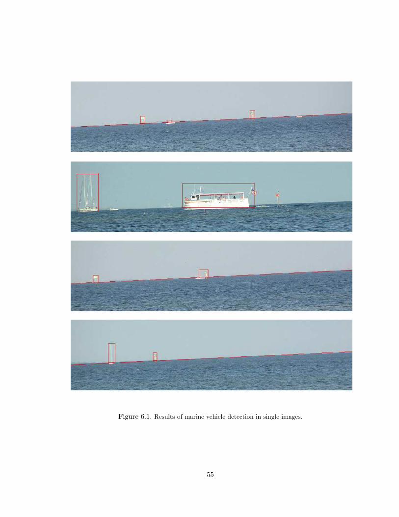
Figure 6.1. Results of marine vehicle detection in single images.

55

Figure 6.2. Examples of ship localization fragmentation. Some of the single-object ships weredetected multiple times causing false alarms.

56

Figure 6.3. Examples of ship detection in video. The picture on the bottom shows an example offailure of detection due to temporal fragmentation of the tracks.

57

CHAPTER 7

CONCLUSIONS

A new technique for automatic detection and tracking of marine vehicles in images and

video of open sea was presented. The proposed computer vision-based algorithm combined

a horizon detection method with edge detection and postprocessing. Several datasets of

still images and video sequences were used to evaluate the performance of the proposed

technique. For video sequences the original algorithm was enhanced by using the Kalman

filter and a tracking algorithm derived from Multiple Hypothesis Framework. Because

the detection algorithm depends on accurate horizon detection, several horizon detection

algorithms were evaluated for accuracy of horizon detection.

Experiments conducted on image and video data showed promising results for marine

vehicle detection and tracking. High detection rate with a moderate alarm rate for low

threshold values was recorded for still images. The visual results for the experiments reflect

the fact that a typical failure for ship detection in a single frame occurs due to multiple

region representation of single objects. This creates a miss result for the original ship and

a false alarm for the attempt. The results suggest that the main cause of failures and false

alarms are edge-detection and postprocessing steps in the original algorithm when a single

object in the sea is represented by several disjoint regions in the postprocessed image.

The main issues with bad tracking performance are related to temporal fragmentation

of tracks. Reducing temporal fragmentation of tracks may lower the false alarm rate

and increase tracking accuracy in the future. Temporal fragmentation in tracking usually

occurs when one track is prematurely terminated because of the long frame-range occlusion

and a new track is started when the watercraft is again visually available. Introducing

58

recognition of objects in separate tracks may be one of the approaches to reduce such

temporal fragmentation.

In future work basic noise removal and color enhancement may be applied for a more

reliable horizon detection which follows image acquisition. An introduction of a training

step in order to identify the parameters of the Canny edge detector may increase the initial

segmentation accuracy and make it adaptable for various daylight conditions. The seg-

mentation accuracy will be improved with an addition of ”merge” procedure, which would

connect closely located segments belonging to one object. One of the possible directions

here is connecting intermittent lines of the contour of marine vehicles using segment finding

techniques described in [44].

The current detection scheme assumes deployment of a buoy in open sea waters and

coastal line was not considered to be present on the horizon. Further direction of the

research may consider this, more complicated environment. Some results on maritime

surveillance in coastal area can be found in [45]. Detection of marine vehicles can be also

paired with marine vehicles classification. Once detected in an image or video sequence a

ship can be classified into a number of categories with methods similar to those mentioned

in the Chapter 1 for FLIR-based images. Determination of the distance to the target may

be another desired functionality following visual detection.

59

REFERENCES

[1] M.I. Skolnik. Introduction to radar systems. McGraw-Hill New York, 1980.

[2] R. Khan, B. Gamberg, D. Power, J. Walsh, B. Dawe, W. Pearson, and D. Millan.Target detection and tracking with a high frequency ground waveradar. OceanicEngineering, IEEE Journal of, 19(4):540–548, 1994.

[3] B. Root. HF radar ship detection through clutter cancellation. Radar Conference,1998. RADARCON 98. Proceedings of the 1998 IEEE, pages 281–286, 1998.

[4] M. Hirota, T. Furuse, K. Ebana, H. Kubo, K. Tsushima, T. Inaba, A. Shima, M. Fu-jinuma, and N. Tojyo. Magnetic detection of a surface ship by an airborne LTS SQUIDMAD. Applied Superconductivity, IEEE Transactions on, 11(1 Part 1):884–887, 2001.

[5] J.C. Curlander and R.N. McDonough. Synthetic aperture radar- Systems and signalprocessing(Book). New York: John Wiley & Sons, Inc., 1991.

[6] M.T. Rey, J.K. Tunaley, J.T. Folinsbee, P.A. Jahans, J.A. Dixon, and M.R. Vant.Application Of Radon Transform Techniques To Wake Detection In Seasat-A SARImages. Geoscience and Remote Sensing, IEEE Transactions on, 28(4):553–560, 1990.

[7] D.R. Thompson and J.R. Jensen. Synthetic aperture radar interferometry appliedto ship-generated internal waves in the 1989 Loch Linnhe experiment. Journal ofGeophysical Research, 98(C6):10259–10270, 1993.

[8] L.M. Murphy. Linear feature detection and enhancement in noisy images via theRadon transform. Pattern Recognition Letters, 4(4):279–284, 1986.

[9] D. Gibbins, DA Gray, and D. Dempsey. Classifying ships using low resolution maritimeradar. Signal Processing and Its Applications, 1999. ISSPA’99. Proceedings of the FifthInternational Symposium on, 1, 1999.

[10] F. Lesage and L. Gagnon. Experimenting level set-based snakes for contour segmen-tation in radar imagery. Proceedings of SPIE, 4041:154, 2000.

[11] P. Valin, Y. Tessier, and A. Jouan. Hierarchical ship classifier for airborne syntheticaperture radar (SAR) images. Signals, Systems, and Computers, 1999. ConferenceRecord of the Thirty-Third Asilomar Conference on, 2, 1999.

[12] C. Yuan and D. Casasent. Composite filters for inverse synthetic aperture radarclassification of small ships. Optical Engineering, 41:94, 2002.

60

[13] V. Gouaillier and L. Gagnon. Ship silhouette recognition using principal componentsanalysis. Proc. SPIE Conf. on Applications of Digital Image Processing XX, 3164:59–69.

[14] C. Alippi. Real-time analysis of ships in radar images with neural networks. PatternRecognition, 28(12):1899–1913, 1995.

[15] Q. Luo, TM Khoshgoftaar, and A. Folleco. Classification of Ships in SurveillanceVideo. Information Reuse and Integration, 2006 IEEE International Conference on,pages 432–437, 2006.

[16] S. Fefilatyev, D.B. Goldgof, and L. Langebrake. Towards detection of marine vehicleson horizon from buoy camera. Proceedings of SPIE, 6736:67360O, 2007.

[17] S. Todorovic. Statistical Modeling and Segmentation of Sky/Ground Images. PhDthesis, Master thesis, University of Florida, 2002.

[18] S.M. Ettinger, M.C. Nechyba, P.G. Ifju, and M. Waszak. Vision-guided flight stabilityand control for micro air vehicles. Advanced Robotics, 17(7):617–640, 2003.

[19] S. Todorovic, MC Nechyba, and PG Ifju. Sky/ground modeling for autonomous MAVflight. Robotics and Automation, 2003. Proceedings. ICRA’03. IEEE InternationalConference on, 1, 2003.

[20] S. Todorovic and MC Nechyba. A vision system for intelligent mission profiles of microair vehicles. Vehicular Technology, IEEE Transactions on, 53(6):1713–1725, 2004.

[21] T. Cornall and G. Egan. Measuring Horizon Angle from Video on a Small UnmannedAir Vehicle, 2004.

[22] T. Cornall and G. Egan. Calculating Attitude from Horizon Vision. Eleventh Aus-tralian International Aerospace Congress, Melbourne, 2005.

[23] G.Q. Bao, S.S. Xiong, and Z.Y. Zhou. Vision-Based Horizon Extraction for Micro AirVehicle Flight Control. Instrumentation and Measurement, IEEE Transactions on,54(3):1067–1072, 2005.

[24] TG McGee, R. Sengupta, and K. Hedrick. Obstacle Detection for Small AutonomousAircraft Using Sky Segmentation. Robotics and Automation, 2005. Proceedings of the2005 IEEE International Conference on, pages 4679–4684, 2005.

[25] S. Fefilatyev, V. Smarodzinava, L.O. Hall, and D.B. Goldgof. Horizon Detection UsingMachine Learning Techniques. Machine Learning and Applications, 2006. ICMLA’06.5th International Conference on, pages 17–21, 2006.

[26] L. Fety, M. Terre, and X. Noreve. Image processing for the detection of the horizonand device for the implemention thereof. United States Patent 5,214,720, ThompsonTRT Defense, 1991.

[27] B. Taylor, C. Bil, S. Watkins, and G. Egan. Horizon Sensing Attitude Stabilisation:A VMC Autopilot. International UAV Systems Conference, Bristol, UK, 2003.

61

[28] M. Sonka, V. Hlavac, and R. Boyle. Image Processing, Analysis, and Machine Vision.2007.

[29] MC Shin, DB Goldgof, and KW Bowyer. Comparison of Edge Detector Performancethrough Use in an Object Recognition Task. Computer Vision and Image Understand-ing, 84(1):160–178, 2001.

[30] M. Shin, D. Goldgof, and KW Bowyer. An objective comparison methodology of edgedetection algorithms using a structure from motion task. Proceedings of CVPR, pages190–195.

[31] J. Canny. A computational approach to edge detection. IEEE Transactions on PatternAnalysis and Machine Intelligence, 8(6):679–698, 1986.

[32] R.C. Gonzalez and R.E. Woods. Digital Image Processing.

[33] R. Jain, R. Kasturi, and B.G. Schunck. Machine vision. McGraw-Hill, Inc. New York,NY, USA, 1995.

[34] G. Welch and G. Bishop. An Introduction to the Kalman Filter. ACM SIGGRAPH2001 Course Notes, 2001.

[35] E. Cuevas, D. Zaldivar, and R. Rojas. Kalman filter for vision tracking.

[36] LC Langebrake, CE Lembke, RH Weisberg, RH Byrne, DR Russell, G. Tilbury, andR. Carr. Design and initial results of a bottom stationing ocean profiler. Oceans’02MTS/IEEE, 1, 2002.

[37] S.J. Pratt. Submarine periscope systems, July 18 1989. US Patent 4,848,886.

[38] D. Reid. An algorithm for tracking multiple targets. Automatic Control, IEEE Trans-actions on, 24(6):843–854, 1979.

[39] I.J. Cox, S.L. Hingorani, et al. An efficient implementation of Reid’s multiple hypoth-esis tracking algorithm and its evaluation for the purpose of visual tracking. IEEETransactions on Pattern Analysis and Machine Intelligence, 18(2):138–150, 1996.

[40] D. Doermann and D. Mihalcik. Tools and techniques for video performance evaluation.Pattern Recognition, 2000. Proceedings. 15th International Conference on, 4, 2000.

[41] R Kasturi, D. Goldgof, P. Soundararajan, V. Manohar, J Garofolo, B. Bowers,M. Boonstra, V. Korzhova, and J. Zhang. Framework for Performance Evaluationof Face, Text, and Vehicle Detection and Tracking in Video: Data, Metrics, andProtocol. IEEE Transactions on Pattern Analysis and Machine Intelligence, pagedoi.ieeecomputersociety.org/10.1109/TPAMI.2008.57.

[42] C.J.C. Burges. A Tutorial on Support Vector Machines for Pattern Recognition. DataMining and Knowledge Discovery, 2(2):121–167, 1998.

[43] N. Littlestone and MK Warmuth. The weighted majority algorithm. Foundations ofComputer Science, 30th Annual Symposium on, pages 256–261.

62

[44] NC Rowe, LL Grewe, U.S.N.P. Sch, and CA Monterey. Change detection for linearfeatures in aerial photographs usingedge-finding. Geoscience and Remote Sensing,IEEE Transactions on, 39(7):1608–1612, 2001.

[45] D.D. Morris, B.R. Colonna, and F.D. Snyder. Image-based motion stabilization formaritime surveillance. Proceedings of SPIE, 6497:64970F, 2007.

63