1

Detection of Compound StructuresUsing a Gaussian Mixture Model with

Spectral and Spatial ConstraintsCaglar Arı and Selim Aksoy, Senior Member, IEEE

Abstract—Increasing spectral and spatial resolution of newgeneration remotely sensed images necessitate the joint useof both types of information for detection and classificationtasks. This paper describes a new approach for the detectionof heterogeneous compound structures such as different typesof residential, agricultural, commercial, and industrial areasthat are comprised of spatial arrangements of primitive objectssuch as buildings, roads, and trees. The proposed approachuses Gaussian mixture models (GMM) in which the individualGaussian components model the spectral and shape charac-teristics of the individual primitives and an associated layoutmodel is used to model their spatial arrangements. We proposea novel expectation-maximization (EM) algorithm that solvesthe detection problem using constrained optimization. The inputis an example structure of interest that is used to estimate areference GMM and construct spectral and spatial constraints.Then, the EM algorithm fits a new GMM to the target imagedata so that the pixels with high likelihoods of being similar tothe Gaussian object models while satisfying the spatial layoutconstraints are identified without any requirement for regionsegmentation. Experiments using WorldView-2 images show thatthe proposed method can detect high-level structures that cannotbe modeled using traditional techniques.

Index Terms—Object detection, Gaussian mixture model,expectation-maximization, constrained optimization, spectral-spatial classification, context modeling

I. INTRODUCTION

Recent increase in both the spatial and the spectral reso-lution of the images acquired from new generation satelliteshave enabled new applications in which the increased spatialresolution brings out objects’ details that were not previouslyvisible and the increased spectral resolution improves thecapability to discriminate the physical characteristics of thesedetails. Consequently, these advances have necessitated newapproaches that effectively exploit both the spectral and thespatial information for the detection and classification ofobjects in these images [1].

A popular approach for joint use of spectral and spatialinformation in the remote sensing literature is to partition theimages into regions and use the spectral properties of the pixelsinside these regions for classification [2], [3], [4]. However,the methods that aim to obtain a smooth classification map

Manuscript received July 30, 2013; revised November 1, 2013. This workwas supported in part by the TUBITAK Grant 109E193. S. Aksoy was alsosupported in part by a Fulbright Visiting Scholar grant.

C. Arı is with the Department of Electrical and Electronics Engineering,Bilkent University, Ankara, 06800, Turkey. Email: cari@ee.bilkent.edu.tr.

S. Aksoy is with the Department of Computer Engineering, Bilkent Uni-versity, Ankara, 06800, Turkey. Email: saksoy@cs.bilkent.edu.tr.

based on homogeneous regions cannot be easily applied to thedetection of a wide range of complex objects such as housingestates, schools, airports, agricultural fields, power plants, andindustrial facilities that have more heterogeneous structures.

An expected component in the approaches that strive todetect such complex objects, called compound structures inthis paper, is a framework that models the spatial arrangementsof simpler primitive objects [5]. Approaches for the detectionof specific structures such as airports [6] and orchards [7]are available. However, these methods are not generalizablebecause they heavily rely on the peculiarities of the objects ofinterest. As a more generic method, Bhagavathy and Manju-nath [8] proposed a window-based detector using histogramsof Gabor texture features, and applied it to the detection of golfcourses and harbors. However, histogram-based methods oftencannot effectively capture the spatial structure. Harvey et al.[9] developed a facility detection framework where the outputsof pixel-based classifiers were used as auxiliary features thatwere input as additional data bands to a final pixel-basedclassifier. They applied this framework to the detection of highschools using athletic fields, parking lots, large buildings, andresidential areas as auxiliary features. However, this frame-work does not explicitly model the spatial arrangements, andneed training data for both the auxiliary and the final detectors.Vatsavai et al. [10] used a latent topic learning algorithmwith spectral, textural, and structural features to categorizeimage tiles as nuclear plants, coal power plants, and airports.However, the tile-based global features often cannot effectivelymodel the geometries or the spatial relationships of the objectsthat comprise the complex structures.

As an example for more explicit modeling of the spatialstructure, Gaetano et al. [11] performed hierarchical texturesegmentation by iteratively merging neighboring regions thathave frequently co-occurring region types. Zamalieva et al.[12] used probabilities estimated from region co-occurrencesto construct the edges of a region adjacency graph, andemployed a graph mining algorithm to find subgraphs thatmay correspond to compound structures. Akcay and Aksoy[13] combined spectral and shape characteristics of primitiveobjects with spatial alignments of neighboring object groupsin assigning weights to the edges of a region adjacencygraph, and then used graph clustering to identify compoundobjects. However, all of these approaches require an initialsegmentation for the identification of the primitive regions, butaccurate segmentation of very high spatial resolution remotelysensed images is still a very difficult problem.

2

Using spatial arrangements of local image primitives hasalso been proven effective for object recognition in the com-puter vision literature [14]. State-of-the-art methods representobject classes in terms of parts that are visually similarand occur in similar spatial configurations. The detection ofparts heavily rely on distinctive invariant features, and theirgrouping is typically handled using combinatorial searchingover all possible part labelings. Popular spatial configurationsinclude the constellation model [15] that is a fully connectedjoint representation of all parts, and the star model [16] thatuses a central reference part and assumes that each part isindependent of the others given this part. However, thesemodels are best suited for objects captured from a consistentviewpoint (e.g., sideways cars, frontal faces) in a large amountof training examples, and are not easily applicable to remotelysensed data that contain thousands of primitive objects thatdo not necessarily generate distinctive features and appear inmany different compositions in the overhead view.

This paper describes a new approach that combines spec-tral and spatial characteristics of simple primitive objects todiscover complex compound structures in very high resolutionimages. The proposed approach uses a probabilistic representa-tion of the image content via Gaussian mixture models (GMM)in which each pixel is represented with a feature vector thatencodes both spectral and spatial information consisting ofthe pixel’s multispectral data and its coordinates, respectively.Each Gaussian component in the GMM models a group ofpixels corresponding to a particular primitive object wherethe spectral mean corresponds to the color of the object, thespectral covariance corresponds to the homogeneity of thecolor content, the spatial mean corresponds to the positionof the object, and the spatial covariance models its shape.

The detection procedure starts with a single example com-pound structure that typically contains a small number ofpixels that are used to estimate a reference GMM. ThisGMM is used to define spectral and spatial constraints foridentifying the occurrences of similar compound structures intarget images. The spectral constraints ensure that the spectralproperties of the detected primitives are similar to those inthe reference model, while the spatial constraints assure thatthe shapes of the detected primitives as well as their spatiallayout defined in terms of relative positions are consistent withthe reference. We formulate the detection task as a constrainedoptimization problem that is solved using a novel expectation-maximization (EM) based algorithm that fits a new GMM tothe target image data and selects groups of pixels that havehigh likelihoods of belonging to the Gaussian object modelswhile satisfying the spatial layout constraints. The proposedapproach has an important feature that it can localize targetstructures without any requirement of an initial segmentation.Furthermore, the pixel-based likelihoods computed via thejoint use of spectral and spatial information can also handlepartial detections and missing primitives, thanks to the con-textual information that the model captures. An early versionof this paper was presented in [17].

The rest of the paper is organized as follows. SectionII defines the proposed compound structure representation.Section III presents the constrained Gaussian mixture model

(a) (b) (c)

Fig. 1. Illustrations of the spectral and spatial parts of an example compoundstructure model containing four buildings with a grass area in the middle anda road nearby. (a) Primitive objects overlayed on the RGB image. (b) Spectralmodel where the gray dots are the pixels’ RGB values and the ellipses showthe spectral parts of the Gaussians corresponding to the primitive objects. (c)Spatial model where the ellipses overlayed on the binary object masks showthe spatial parts of the Gaussians corresponding to the primitive objects andthe lines represent the layout model. Note that each primitive object has acorresponding Gaussian in the full spectral-spatial feature space.

that is used to model this representation. Section IV de-scribes the EM-based maximum likelihood detection algorithmfor finding similar structures in target images. Section Vpresents experimental results using multispectral WorldView-2imagery. Finally, Section VI provides our conclusions.

II. DEFINITION OF COMPOUND STRUCTURES

In this paper, compound structures are defined as high-level heterogeneous objects that are composed of spatial ar-rangements of multiple, relatively homogeneous, and compactprimitive objects. To build the model for these structures,first, each pixel is represented by using a d-dimensionalfeature vector x = (xms; xxy) where x ∈ Rd is formedby concatenating a d − 2 dimensional vector xms contain-ing the multispectral values and a 2-dimensional vector xxy

containing the pixel’s coordinates in the image. Since eachprimitive object is assumed to have a relatively homogeneousspectral content and a compact shape, we further assume thatit can be modeled using a Gaussian that is defined in terms ofthe mean µ = (µms;µxy) and the block diagonal covariancematrix Σ = (Σms, 0; 0,Σxy). The covariance model assumesthat the multispectral values and the pixel coordinates areindependent, i.e., p(x) = p(xms)p(xxy), which is similar tothe common assumption about the independence of appearanceand geometry in the state-of-the-art part-based object detectors[14]. Given a group of pixels forming the primitive object,the spectral mean µms corresponds to the average colorof the object, the spectral covariance Σms corresponds tothe homogeneity of the color content, the spatial mean µxy

corresponds to the position of the object, and the spatialcovariance Σxy models its shape as a convex object. Figure 1illustrates the spectral and spatial parts of an example model.

A compound structure consisting of K primitive objects canthen be modeled using a Gaussian mixture model (GMM)

p(x|Θ) =

K∑k=1

αkpk(x|µk,Σk) (1)

that is fully defined by the set of parameters Θ =αk,µk,ΣkKk=1 where µk ∈ Rd denotes the mean vectorand Σk ∈ Sd++ denotes the covariance matrix of the k’th

3

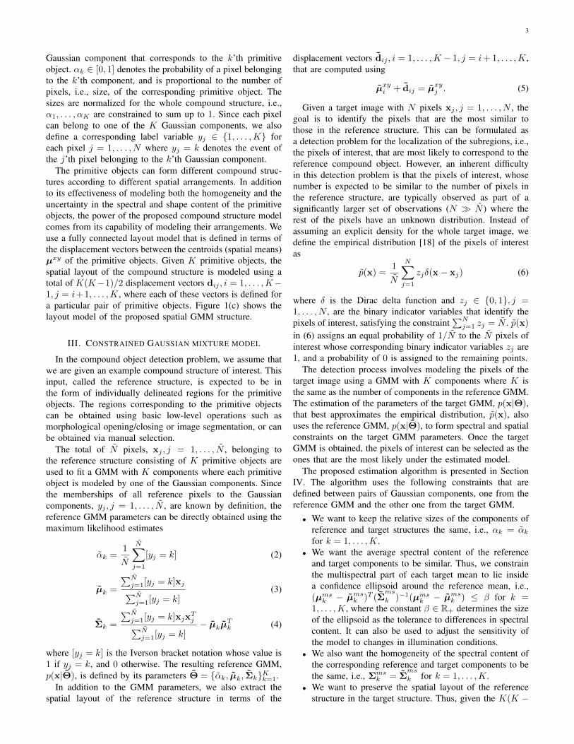
Gaussian component that corresponds to the k’th primitiveobject. αk ∈ [0, 1] denotes the probability of a pixel belongingto the k’th component, and is proportional to the number ofpixels, i.e., size, of the corresponding primitive object. Thesizes are normalized for the whole compound structure, i.e.,α1, . . . , αK are constrained to sum up to 1. Since each pixelcan belong to one of the K Gaussian components, we alsodefine a corresponding label variable yj ∈ 1, . . . ,K foreach pixel j = 1, . . . , N where yj = k denotes the event ofthe j’th pixel belonging to the k’th Gaussian component.

The primitive objects can form different compound struc-tures according to different spatial arrangements. In additionto its effectiveness of modeling both the homogeneity and theuncertainty in the spectral and shape content of the primitiveobjects, the power of the proposed compound structure modelcomes from its capability of modeling their arrangements. Weuse a fully connected layout model that is defined in terms ofthe displacement vectors between the centroids (spatial means)µxy of the primitive objects. Given K primitive objects, thespatial layout of the compound structure is modeled using atotal of K(K−1)/2 displacement vectors dij , i = 1, . . . ,K−1, j = i+1, . . . ,K, where each of these vectors is defined fora particular pair of primitive objects. Figure 1(c) shows thelayout model of the proposed spatial GMM structure.

III. CONSTRAINED GAUSSIAN MIXTURE MODEL

In the compound object detection problem, we assume thatwe are given an example compound structure of interest. Thisinput, called the reference structure, is expected to be inthe form of individually delineated regions for the primitiveobjects. The regions corresponding to the primitive objectscan be obtained using basic low-level operations such asmorphological opening/closing or image segmentation, or canbe obtained via manual selection.

The total of N pixels, xj , j = 1, . . . , N , belonging tothe reference structure consisting of K primitive objects areused to fit a GMM with K components where each primitiveobject is modeled by one of the Gaussian components. Sincethe memberships of all reference pixels to the Gaussiancomponents, yj , j = 1, . . . , N , are known by definition, thereference GMM parameters can be directly obtained using themaximum likelihood estimates

αk =1

N

N∑j=1

[yj = k] (2)

µk =

∑Nj=1[yj = k]xj∑Nj=1[yj = k]

(3)

Σk =

∑Nj=1[yj = k]xjx

Tj∑N

j=1[yj = k]− µkµ

Tk (4)

where [yj = k] is the Iverson bracket notation whose value is1 if yj = k, and 0 otherwise. The resulting reference GMM,p(x|Θ), is defined by its parameters Θ = αk, µk, ΣkKk=1.

In addition to the GMM parameters, we also extract thespatial layout of the reference structure in terms of the

displacement vectors dij , i = 1, . . . ,K − 1, j = i+ 1, . . . ,K,that are computed using

µxyi + dij = µxy

j . (5)

Given a target image with N pixels xj , j = 1, . . . , N , thegoal is to identify the pixels that are the most similar tothose in the reference structure. This can be formulated asa detection problem for the localization of the subregions, i.e.,the pixels of interest, that are most likely to correspond to thereference compound object. However, an inherent difficultyin this detection problem is that the pixels of interest, whosenumber is expected to be similar to the number of pixels inthe reference structure, are typically observed as part of asignificantly larger set of observations (N N ) where therest of the pixels have an unknown distribution. Instead ofassuming an explicit density for the whole target image, wedefine the empirical distribution [18] of the pixels of interestas

p(x) =1

N

N∑j=1

zjδ(x− xj) (6)

where δ is the Dirac delta function and zj ∈ 0, 1, j =1, . . . , N , are the binary indicator variables that identify thepixels of interest, satisfying the constraint

∑Nj=1 zj = N . p(x)

in (6) assigns an equal probability of 1/N to the N pixels ofinterest whose corresponding binary indicator variables zj are1, and a probability of 0 is assigned to the remaining points.

The detection process involves modeling the pixels of thetarget image using a GMM with K components where K isthe same as the number of components in the reference GMM.The estimation of the parameters of the target GMM, p(x|Θ),that best approximates the empirical distribution, p(x), alsouses the reference GMM, p(x|Θ), to form spectral and spatialconstraints on the target GMM parameters. Once the targetGMM is obtained, the pixels of interest can be selected as theones that are the most likely under the estimated model.

The proposed estimation algorithm is presented in SectionIV. The algorithm uses the following constraints that aredefined between pairs of Gaussian components, one from thereference GMM and the other one from the target GMM.• We want to keep the relative sizes of the components of

reference and target structures the same, i.e., αk = αk

for k = 1, . . . ,K.• We want the average spectral content of the reference

and target components to be similar. Thus, we constrainthe multispectral part of each target mean to lie insidea confidence ellipsoid around the reference mean, i.e.,(µms

k − µmsk )T (Σ

ms

k )−1(µmsk − µms

k ) ≤ β for k =1, . . . ,K, where the constant β ∈ R+ determines the sizeof the ellipsoid as the tolerance to differences in spectralcontent. It can also be used to adjust the sensitivity ofthe model to changes in illumination conditions.

• We also want the homogeneity of the spectral content ofthe corresponding reference and target components to bethe same, i.e., Σms

k = Σms

k for k = 1, . . . ,K.• We want to preserve the spatial layout of the reference

structure in the target structure. Thus, given the K(K −

4

µms1

Σms1

µms2

Σms2

µms3

Σms3

(a)

µms1µms

2

µms3

(b)

Σms1Σms

2

Σms3

(c)

Fig. 2. Spectral constraints for an example mixture of three Gaussians. (a)Reference spectral model. (b) Mean constraints: means must lie inside theellipsoids defined as (µms

k − µmsk )T (Σ

msk )−1(µms

k − µmsk ) ≤ β. (c)

Covariance constraints: Σmsk = Σ

msk .

µxy1

Σxy1

µxy2

Σxy2

µxy3

Σxy3

(a)

µxy1 µxy

2

µxy3

d12

d13 d23

t12 t13

t23

(b)

Σxy1 Σxy

2

Σxy3

(c)

Fig. 3. Spatial constraints for an example mixture of three Gaussians. (a)Reference spatial model. (b) Mean constraints: means must lie inside thesquares defined as µxy

i +dij−µxyj = tij , ‖tij‖1 ≤ u where µxy

i +dij =

µxyj . (c) Covariance constraints: aspect ratios are preserved while rotations

are allowed as λmin (Σxyk ) = λmin (Σ

xyk ) and λmax (Σ

xyk ) = λmax (Σ

xyk ).

1)/2 displacement vectors dij , i = 1, . . . ,K− 1, j = i+1, . . . ,K, that are computed as in (5), the spatial layout ofthe target structure is constrained as µxy

i +dij−µxyj = tij

where ‖tij‖1 ≤ u and the constant u ∈ R+ specifies theallowed amount of deviation from the reference spatialrelations.

• Finally, we want the aspect ratio of each reference prim-itive object to be preserved in the target. Thus, we con-strain the minimum and maximum eigenvalues, λmin andλmax , respectively, of the spatial parts of the referenceand target covariances to be the same, i.e., λmin(Σxy

k ) =

λmin(Σxy

k ) and λmax (Σxyk ) = λmax (Σ

xy

k ) for k =1, . . . ,K. Note that this allows different rotations of theprimitive objects.

The spectral and spatial constraints are illustrated in Figures2 and 3, respectively.

IV. DETECTION ALGORITHM

The input to the detection problem is the reference GMM,p(x|Θ), that is estimated from N pixels in the referencecompound structure, and a target image containing N pixels,x1, . . . ,xN , among which an unknown subset of size Nconstitutes the pixels of interest that are assumed to havethe empirical distribution, p(x). We do not make any explicitassumption about the distribution of the remaining N − Npixels in the target image.

The goal of the detection algorithm is to estimate theparameters of the target GMM, p(x|Θ), that best approxi-mates the empirical distribution, p(x). In information theory,

the relative entropy or the Kullback-Leibler (KL) divergence[19] is a widely used measure of dissimilarity between twoprobability distributions p(x) and p(x). It can be interpretedas the additional amount of information required to specify thevalue of x as a result of using p instead of the true distributionp, and is computed as

KL(p‖p) =

∫p(x) log

p(x)

p(x)dx

=

∫p(x) log p(x)dx−

∫p(x) log p(x)dx

= −H(p(x))−∫p(x) log p(x)dx

(7)

where H(p(x)) denotes the differential entropy of the proba-bility distribution p(x). The detection problem in this paper isformulated as the minimization of the KL divergence betweenp(x) and p(x|Θ) over the constrained GMM parameters Θand the indicator variables Z = z1, . . . , zN as

Θ∗,Z∗ = arg minΘ,Z

KL(p(x)‖p(x|Θ)). (8)

Using (7), we can expand the KL divergence in (8) as

KL(p(x)‖p(x|Θ))

= −H(p(x))−∫

1

N

N∑j=1

zjδ(x− xj) log p(x|Θ)dx

= −H(p(x))− 1

N

N∑j=1

zj log p(xj |Θ).

(9)

Since H(p(x)) does not depend on the parameters Θ andthe indicator variables Z due to the constraint that they sumto N (the entropy does not change according to which Nzj among N are set to 1), the objective (9) corresponds tothe minimization of the negative weighted log-likelihood, orequivalently, maximization of the weighted log-likelihood as

Θ∗,Z∗ = arg maxΘ,Z

N∑j=1

zj log p(xj |Θ). (10)

Since the objective function in (10) is not jointly concavein Θ and Z , there is no algorithm that can guarantee to findthe global optimum. However, the GMM parameters and theindicator variables that correspond to a local optimum solutionof (10) can be obtained via alternating optimization using anexpectation-maximization (EM) based algorithm.

The EM algorithm uses distributions over the unobservedlabel variables to obtain a lower bound for the original log-likelihood function. Let W = wjk = P (yj = k|xj ,Θ), j =1, . . . , N, k = 1, . . . ,K denote the posterior probabilities ofthe label variables given the corresponding data points xj , j =1, . . . , N . A lower bound function F (Z,W,Θ) for the log-

5

likelihood function l(Z,Θ) can be obtained as

l(Z,Θ) =

N∑j=1

zj log

( K∑k=1

αkpk(xj |µk,Σk)

)

=

N∑j=1

zj log

( K∑k=1

wjkαkpk(xj |µk,Σk)

wjk

)

≥N∑j=1

zj

K∑k=1

wjk log

(αkpk(xj |µk,Σk)

wjk

)(using Jensen’s inequality)

=

N∑j=1

zj

K∑k=1

wjk

(log(αkpk(xj |µk,Σk))− log(wjk)

)= F (Z,W,Θ).

(11)

Then, the auxiliary optimization problem that uses the derivedlower bound can be written as

maximize F (Z,W,Θ) over Z,W,Θ

subject toK∑

k=1

wjk = 1, j = 1, . . . , N,

zj ∈ 0, 1, j = 1, . . . , N,N∑j=1

zj = N ,

Θ ∈ CΘ

(12)

where CΘ is the constraint set for Θ as defined in SectionIII. Note that this problem can be solved by introducing arelaxation of the binary indicator variables zj ∈ 0, 1, j =1, . . . , N as 0 ≤ zj ≤ 1 where an optimal solution still consistsof binary values as described below.

The proposed algorithm uses alternating optimization to finda local optimum solution where F (Z,W,Θ) is maximizedover Z for fixed W and Θ, and over W and Θ for fixed Ziteratively. For fixedW and Θ, the objective function becomeslinear in Z , and maximization of a linear objective over a unitbox with a total sum constraint corresponds to a linear programwith a simple solution: zj = 1 for the N data points with thelargest

∑Kk=1 wjk

(log(αkpk(xj |µk,Σk))− log(wjk)

)values

and zj = 0 for the rest. We call this the Z-step.For fixed Z , the solutions for W and Θ are similar to

the conventional EM algorithm for GMM estimation. If therewere no constraints on Θ, the update equations for the GMMparameters for the optimization of F (Z,W,Θ) via the EMiterations can be derived as

w(t)jk =

α(t)k pk(xj |µ(t)

k ,Σ(t)k )∑K

i=1 α(t)i pi(xj |µ(t)

i ,Σ(t)i )

(13)

α(t+1)k =

∑Nj=1 zjw

(t)jk∑K

i=1

∑Nj=1 zjw

(t)ji

(14)

µ(t+1)k =

∑Nj=1 zjw

(t)jk xj∑N

j=1 zjw(t)jk

(15)

Σ(t+1)k =

∑Nj=1 zjw

(t)jk xjx

Tj∑N

j=1 zjw(t)jk

− µ(t+1)k

(µ

(t+1)k

)T(16)

where (13) corresponds to the E-step, (14)–(16) correspondto the M-step, and the index t corresponds to the iterationnumber. However, the parameters might not satisfy the desiredconstraints after being updated in the M-step. Thus, to handlethe constraints that are defined with respect to the referenceGMM in the previous section, we project the parameters ontoconstraint sets at the end of every iteration. This can be consid-ered as a special case of the alternating projections algorithmfor handling constrained optimization problems [20].

We use the square of the Euclidean distance to measure thedistance of a point θ ∈ Ω to a constraint set Cθ ⊆ Ω where

dist(θ, Cθ) = min‖θ − θ‖22 | θ ∈ Cθ (17)

and Ω is the domain of θ. The point θ ∈ Cθ that is closest toθ, i.e., the point for which the minimum in (17) is attained, isreferred to as the projection of θ on Cθ. We use PCθ : Ω→ Cθto denote the projection function onto the constraint set Cθ,and PCθ (θ) as the projection of θ on Cθ. Projections PCθ (θ)are computed by solving optimization problems defined bythe selected constraints. Some of the optimization problems ofinterest are easy to solve and have simple analytical solutions.However, in general, no analytical solution exists but a solutioncan be obtained very efficiently using interior point or activeset algorithms [21], [22].

The parameters in Θ that satisfy the particular constraintsdefined in Section III can be computed as follows. The priorprobabilities can be obtained as the solution of

minimizeK∑

k=1

|αk − αk|2

subject to αk = αk, k = 1, . . . ,K.

(18)

Due to the equality constraints, the optimal value of (18) isachieved with αk = αk for k = 1, . . . ,K.

Next, the optimization problem and the correspondingprojection operator PCΣ for finding the projections of thecovariance matrices is defined as

minimizeK∑

k=1

‖Σk − Σk‖22

subject to Σmsk = Σ

ms

k , k = 1, . . . ,K,

λmin(Σxy

k )I2 ≤ Σxyk ≤ λmax (Σ

xy

k )I2,

k = 1, . . . ,K,

Σik = 0 for i 6= ms, i 6= xy, k = 1, . . . ,K

(19)

where I2 is the 2-by-2 identity matrix. The optimal solutionfor (19) is computed by setting Σms

k = Σms

k , Σik = 0 for i 6=

ms and i 6= xy, and doing eigenvalue decomposition on thespatial part of Σ

(t+1)k , thresholding the eigenvalues according

to the max-min limits, and reconstructing the spatial part ofΣ

(t+1)k using the clipped eigenvalues and eigenvectors.Finally, the projections of the mean vectors, PCµ , are

computed by solving the following quadratic programming

6

loglikelihood = 0.0000000000 loglikelihood = −8761.5334007717 loglikelihood = −8531.7557982387 loglikelihood = −8228.1839516843 loglikelihood = −7935.5245573091 loglikelihood = −7103.7408145250

(a)loglikelihood = −8873.3172302310 loglikelihood = −7353.8152933238 loglikelihood = −6941.4137925422 loglikelihood = −6505.0687125811 loglikelihood = −5979.7247185702 loglikelihood = −5890.7011283430

(b)loglikelihood = −6156.1146788613 loglikelihood = −6308.2627675255 loglikelihood = −5882.3233290240 loglikelihood = −5654.4957065098 loglikelihood = −5397.9257465936 loglikelihood = −5233.6136998201

(c)

Fig. 4. Illustration of the convergence of the EM iterations using the reference structure in Figure 5(b). Each row shows a different run with a particularinitialization. Each figure shows a particular iteration where the magenta circles are the initial locations of the Gaussians in the first iteration, the cyan dotsmark the pixels selected at the end of the Z step, and the yellow ellipses show the current versions of the Gaussians at the end of the M step. The last columnshows the solution corresponding to the run in that row. (a) Iterations 1, 16, 32, 48, 64, and 80 are shown. The final log-likelihood was −7103. (b) Iterations1, 3, 6, 9, 13, and 22 are shown. The final log-likelihood was −5890. (c) Iterations 1, 4, 15, 23, 30, and 38 are shown. The final log-likelihood was −5233.The likelihood values proved to be reliable indicators of the goodness of the solutions with increasing fitness values from (a) to (c).

problem:

minimizeK∑

k=1

‖µk − µk‖22

subject to (µmsk − µms

k )T (Σms

k )−1(µmsk − µms

k ) ≤ β,k = 1, . . . ,K,

µxyi + dij − µxy

j = tij , ‖tij‖1 ≤ u,i = 1, . . . ,K − 1, j = i+ 1, . . . ,K.

(20)

The proposed detection algorithm is summarized in Algo-rithm 1. The EM procedure is run by starting from differentinitializations (described in Section V-B) of the target GMMon the target image. Each run with a particular initializationfinds a solution to (12) by alternating between the E, Z, andM steps until an allowed maximum number of iterations isattained or until the difference between the log-likelihoodvalues at two successive iterations falls below some giventhreshold. The result of each run is the GMM parametersΘ∗ and the indicator variables Z∗ corresponding to a localmaximum of the weighted log-likelihood function in (10).Each result involves the binary indicator variables zjNj=1

among which N are 1 and N − N are 0, and corresponds toa grouping (selection) of the pixels that have high likelihoodsof being similar to the reference Gaussian object model whilesatisfying the spatial layout constraints. The correspondinglikelihood value is considered as a measure of the goodness ofthat result. The final detection score for each pixel is obtainedas the highest likelihood value among the runs in which itis selected. Figure 4 illustrates the convergence of the EMiterations for different initializations.

Algorithm 1 Compound object detection algorithm

Input: xjNj=1, αk, µk, ΣkKk=1, dijK−1,Ki=1,j=i+1, β, u, NOutput: detection scores sjNj=1

1: sj ← −∞2: for all initializations in the image do3: t← 04: Set α(0)

k ,µ(0)k ,Σ

(0)k

5: repeat EM iterations6: E-step: compute w(t)

jk using (13)7: Z-step: zj ← 1 for N data points with

largest∑K

k=1 w(t)jk

(log(α

(t)k pk(xj |µ(t)

k ,Σ(t)k ))−

log(w(t)jk ))

and zj ← 0 for others8: M-step: compute α

(t+1)k ,µ

(t+1)k ,Σ

(t+1)k using

(14)–(16)9: Projection: update α

(t+1)k ,µ

(t+1)k ,Σ

(t+1)k by

solving (18)–(20)10: t← t+ 111: until maximum number of iterations reached or log-

likelihood unchanged12: sj ← maxsj , log-likelihood,∀j such that zj = 113: end for

V. EXPERIMENTS

A. Data sets

The experiments were performed using multispectralWorldView-2 images of Ankara and Kusadasi in Turkey. Inparticular, the Ankara data consisted of a subscene with asize of 700 × 700 pixels and 2 m spatial resolution cover-

7

ing a residential area with various groups of buildings withdifferent shapes and arrangements as shown in Figure 5(a).The Kusadasi data consisted of two subscenes, each with asize of 600× 600 pixels and 2 m spatial resolution, coveringalso residential areas with different types of building groupsas shown in Figures 6(a) and 6(e).

B. Experimental protocolThe input reference compound structures used in the exper-

iments were obtained by manual delineation of the individualprimitive objects. This can be considered a very moderaterequirement as only a few individual objects need to bedelineated as opposed to relatively large training sets neededfor supervised detection and classification algorithms. Givena single example structure, the parameters of the referenceGaussian components in p(x|Θ) were obtained via maximumlikelihood estimation using the pixels belonging to each primi-tive object. In particular, the component probabilities αkKk=1

were estimated using the ratio of the number of pixels in eachprimitive object to the total number of pixels in the compoundstructure as in (2), and the means µkKk=1, the covariance ma-trices ΣkKk=1, and the displacement vectors dijK−1,Ki=1,j=i+1

were estimated as in (3), (4), and (5), respectively.After this step with a user input, the rest of the detection

process was performed fully unsupervised using the EM algo-rithm described in Section IV. Note that, the algorithm workson individual pixels without requiring any initial segmentationwhile performing object detection, but at the same time hasthe capability of grouping individual pixels that have highlikelihoods of belonging to the Gaussian object models whilesatisfying the spatial layout constraints.

In the EM algorithm, the parameters of the target GMMp(x|Θ) were initialized by using the parameters of the refer-ence model. First of all, the number of mixture components(K) was fixed at the number of primitive objects in the ref-erence structure. Next, the Gaussian component probabilitiesαkKk=1 were initialized to the reference Gaussian componentprobabilities. Similarly, the spectral means µms

k Kk=1 and co-variances Σms

k Kk=1 were initialized to the reference GMM’scorresponding means and covariances.

Since each different initialization of the EM algorithmconverges to a local maximum of the likelihood function andthere is no prior information about the expected locations ofcompound structures of interest in the target image, we used astraightforward initialization procedure for the spatial meansµxy

k Kk=1 using uniform sampling of the image coordinates.A grid of pixels with row and column increments of 20 pixelsand a buffer of 30 pixels at the image boundaries was used asoffsets to be added to the spatial means of the reference objectswhile preserving the displacement relations of the spatialmeans computed from the reference GMM (three exampleswere given in Figure 4). This resulted in 32×32 = 1024 runsfor the EM algorithm for the Ankara image, and 27×27 = 729runs for each of the Kusadasi images. For each run, thespatial covariances Σxy

k Kk=1 were initialized to the referenceGMM’s corresponding spatial covariances.

Each EM run solved the optimization problem in (12) withthe stopping condition selected to be the difference between

the log-likelihood values at two consecutive iterations beingless than 10−9 or a maximum of 100 iterations. Regardingthe parameters in the constraints, β in Figure 2 was setto 10−9, and the deformation parameter u in Figure 3 wasset as 0.1 or 10 pixels for a strict or loose satisfaction,respectively, of the spatial layout constraints. Finally, thenumber of pixels of interest (N ) was set to the total numberof pixels in the reference structure. This choice correspondedto the expectation that the structures of interest in the targetimage had a similar scale as the reference structure. Detectionof structures at scales different from the reference structureis straightforward by scaling N and the parameters of thereference model (spatial means, covariances, and displacementvectors) accordingly. Rotations of the reference structure at 45and 90 degrees were considered in the experiments below.

C. Baseline for comparison

The baseline method that was used for comparison was theunconstrained Gaussian mixture classifier. The first baselineresult (referred to as GMM1) was obtained by computingthe likelihood of each pixel using its multispectral valuesas∑K

k=1 αkpk(xms|µmsk , Σ

ms

k ) using the GMM estimatedfrom the input reference structure. The second baselineresult (referred to as GMM2) was obtained by assigningthe highest probability given by individual reference Gaus-sian components as the detection score of each pixel asmaxK

k=1 αkpk(xms|µmsk , Σ

ms

k ). Both of these methods arewidely used for GMM-based classification of remotely sensedimages in the literature.

D. Evaluation criteria

Thresholding of the detection score at each pixel producesa binary detection map. We used precision and recall as thequantitative performance criteria as in [7] to compare thebinary detection maps obtained using a uniformly sampledrange of thresholds to the validation data that were obtained bymanual labeling of the structures of interest as positive and therest of the image as negative. Recall (producer’s accuracy), thatis computed as the ratio of the number of correctly detectedpixels to the number of all pixels in the validation data, canbe interpreted as the number of true positives detected by thealgorithm, while precision (user’s accuracy), that is computedas the ratio of the number of correctly detected pixels tothe number of all detected pixels, evaluates the algorithm’stendency for false positives. We also used the F-measure thatcombines precision and recall using their harmonic mean as

F =2× precision× recall

precision + recall(21)

to rank different experimental settings and determine thebest threshold. A particular threshold value can be selectedinteractively or by using automatic thresholding techniques[23] when no validation data are available.

In addition to pixel-based evaluation, we also performedobject-based evaluation as in [24]. This strategy, called focus-of-attention, assumes that a single correctly detected pixelinside a target object is sufficient to attract the operator’s

8

attention to that target and label it as correctly detected, butany pixel outside the target is a false alarm because it divertsattention away from true targets. In our implementation ofthe focus-of-attention strategy, we used the convex hull of thepixels belonging to each structure of interest as the objectmask for that structure. Then, given the binary detection mapfor a particular threshold, the union of one or more pixelsinside the mask of a target structure was counted as a truepositive, while the number of connected components of pixelsthat did not overlap with any target structure was counted asfalse positives. Precision and recall used counts of groups ofpixels instead of individual pixels for object-based evaluation.

E. Results

The proposed object detection algorithm was evaluatedusing two scenarios. The first scenario aimed the detection ofa structure composed of four buildings with red roofs placedin a diamond formation in the Ankara image as shown inFigure 5. The second scenario aimed the detection of a housingestate composed of four buildings and a pool in the Kusadasiimages as shown in Figure 6. Since all three WorldView-2test images contained suburban scenes, the detection scenariosmainly involved the detection of building groups.

The first set of experiments was done to evaluate the effectsof combinations of different rotations of the reference structurein the detection performance as shown in Figure 7. 0 and45 degree rotations were considered for the Ankara image,whereas 0, 45, and 90 degree rotations were considered forthe Kusadasi images as shown in Figures 5 and 6 (0 degreemeans no rotation). The final detection score for a combinationwas obtained as the pixelwise maximum of the scores obtainedby using individual structures. The results showed that usingmultiple rotations of the reference structure could improve theperformance depending on the image content. For example,the best performance in terms of the F-measure was obtainedwith the original reference structure (0 degrees) for the Ankaraimage. However, combining 0 and 90 degree rotations gavethe best results for the Kusadasi1 image, and combining 0,45, and 90 degree rotations gave the best results for theKusadasi2 image. These results were reasonable consideringthe appearances of the target structures in the validation datashown in Figures 5 and 6. Note that different rotations of thereference structure affect only the displacement vectors in thelayout model as rotations of individual primitive objects werealready allowed in the constraints. According to the varianceof the F-measure resulting from different combinations, themodel with u = 0.1 was affected slightly more than themodel with u = 10 from different combinations. This wasalso expected because larger amounts of deformations wereallowed in the latter model but the former required a morestrict satisfaction of the layout constraints.

The next set of experiments was done to compare the per-formances of the proposed detection algorithm (referred to asCGMM) and the baseline methods (referred to as GMM1 andGMM2) as described in Sections V-B and V-C, respectively.Figure 8 shows the pixel likelihoods as the detection scoresfor all methods for all images. The best rotation combinations

TABLE IPRECISION, RECALL AND F VALUES FOR THE BEST PERFORMANCE FOR

DIFFERENT DETECTION METHODS AND DATA SETS. THE BESTPERFORMANCE CORRESPONDS TO THE LIKELIHOOD THRESHOLD THAT

OBTAINED THE HIGHEST F VALUE.

Pixel-based Object-basedData Method Prec. Rec. F Prec. Rec. F

Ank

ara CGMM (u=0.1) 0.9782 0.5292 0.6868 1.0000 0.7500 0.8571

CGMM (u=10) 0.9956 0.6932 0.8173 1.0000 1.0000 1.0000GMM1 0.1366 0.3737 0.2000 1.0000 0.2500 0.4000GMM2 0.1390 0.4036 0.2068 0.0103 1.0000 0.0204

Kus

adas

i1 CGMM (u=0.1) 0.4619 0.5372 0.4967 0.7692 0.7692 0.7692CGMM (u=10) 0.4269 0.4783 0.4512 1.0000 0.5385 0.7000

GMM1 0.0410 0.4175 0.0746 0.0187 0.5385 0.0362GMM2 0.0412 0.4104 0.0749 0.0186 0.5385 0.0360

Kus

adas

i2 CGMM (u=0.1) 0.5405 0.5278 0.5341 0.7222 0.9286 0.8125CGMM (u=10) 0.5071 0.5522 0.5287 0.9231 0.8571 0.8889

GMM1 0.0949 0.1170 0.1048 0.0267 0.6429 0.0513GMM2 0.0846 0.1347 0.1039 0.0269 0.6429 0.0517

from Figure 7 were used for the CGMM results. The resultsshowed that the proposed algorithm could provide a very goodlocalization of the target structures of interest by incorporatingboth spectral and structural information in the constrainedGMM models. The relative likelihood values were also verystrong indicators of the goodness of the detection as the highestlikelihood values were obtained for the pixels that belonged tothe objects that were very similar to the individual primitivesin the reference structures but also satisfied the spatial layoutconstraints. The spatial constraints that allowed rotations ofindividual primitives also enabled the detection of additionalstructures involving cross-like formations or parallel groupsof buildings as well as rotated pools while preserving therelative displacements computed from the reference GMMs.On the other hand, the baseline methods that did not useany spatial information detected a wide range of individualobjects without any consideration of their spatial arrangementsas expected. This led to very low precision and unsatisfactorylocalization of the structures of interest.

Figure 9 shows precision versus recall curves obtained byapplying different threshold values to the likelihood baseddetection scores, and Table I summarizes the results corre-sponding to the best thresholds. The results showed that theproposed algorithm that jointly exploited spectral and spatialinformation performed significantly better than the baselinemethods that only used spectral information. In particular,CGMM achieved significantly higher precision values thanGMM1 and GMM2 for the same value of recall for both pixel-based and object-based evaluation. There was no significantdifference between the performances of GMM1 and GMM2,but the accuracies of the models with u = 0.1 and u = 10varied according to the appearances of the target structuresof interest in different images. For example, the model withu = 10 performed significantly better than the one withu = 0.1 in the Ankara image because of the flexibilityneeded in the displacement of the primitive objects in thetarget structures of interest. However, for the Kusadasi images,the model with u = 10 obtained slightly higher precisionscores for very high values of recall whereas the model withu = 0.1 often had slightly higher precision scores for lower

9

(a) (b) (c) (d)

Fig. 5. Target structure composed of four buildings with red roofs in a diamond formation in the Ankara image. (a) RGB image. (b) Close-up (as a 50× 50pixel patch) of the reference structure used in the detection algorithm with the primitive objects overlayed as yellow polygons and the corresponding referenceGMMs at 0 and 45 degree rotations. (c) Validation data used for pixel-based evaluation with the individual primitive objects overlayed as yellow. (d) Validationdata used for object-based evaluation with the convex hulls of the target structures overlayed as yellow.

(a) (b) (c) (d)

(e) (f) (g) (h)

Fig. 6. Target structure composed of a housing estate with four buildings and a pool in the Kusadasi images. (a,e) RGB images (Kusadasi1 and Kusadasi2).(b,f) Close-up (as a 50× 50 pixel patch) of the reference structure (from (a)) used in the detection algorithm with the primitive objects overlayed as yellowpolygons and the corresponding reference GMMs at 0, 45, and 90 degree rotations. (c,g) Validation data used for pixel-based evaluation with the individualprimitive objects overlayed as yellow. (d,h) Validation data used for object-based evaluation with the convex hulls of the target structures overlayed as yellow.

0

0.1

0.2

0.3

0.4

0.5

0.6

0.7

0.8

0.9

1

10 01 11

(a)

0

0.1

0.2

0.3

0.4

0.5

0.6

0.7

100 010 001 110 101 011 111

(b)

0

0.1

0.2

0.3

0.4

0.5

0.6

0.7

100 010 001 110 101 011 111

(c)

Fig. 7. Precision, recall, and F values for combinations of different rotations of the reference structure. The binary codes below the plots indicate the rotationsettings used for each result: 0 and 45 degrees for the Ankara image in (a), and 0, 45, and 90 degrees for the Kusadasi1 and Kusadasi2 images in (b) and(c), respectively. Precision, recall, and F values (from left to right) are shown as red and blue bars for u = 0.1 and u = 10, respectively, for each setting.

10

Fig. 8. Pixel likelihoods as detection scores. Brighter values indicate higher likelihoods. The first column shows the RGB images, the second and the thirdcolumns show the results for CGMM using u = 0.1 and u = 10, respectively, and the fourth column shows the results for GMM2. The results for GMM1were very similar to those of GMM2. Note that the likelihood values for the proposed model were very discriminative and provided good localization.

recall values. This could be explained with the observationthat the more strict model (u = 0.1) needed to produce moredetections to achieve very high recall values but could be moreselective when missing some of the targets could be tolerated.The performance scores for the Ankara image were higher ingeneral than the scores for the Kusadasi images because thetarget primitive objects of interest in the Ankara image had anaverage size of 120 pixels whereas the target primitives in theKusadasi images had an average size of 13 pixels, making thelatter a much more difficult learning and detection task. Theresults also showed that object-based performance scores werealways higher than those in pixel-based evaluation. This wasconsistent with the observations in [24] that the object-basedtarget detection evaluation permits a much higher thresholdthan would be needed to accurately detect most of the pixelsin the target, and an increased threshold generally producesfewer false alarms.

Figure 10 shows detection examples. Considering that theprimitive objects in the input structures used to estimate thereference GMMs had on average only 80 and 16 pixels forthe Ankara (Figure 5) and Kusadasi (Figure 6) images, respec-tively, the detection results by the proposed method showed avery effective localization of the target structures. For example,even though the spectral-only GMM1 and GMM2 models

could not learn and detect the pools in the Kusadasi images,the proposed model could identify most of the pools becauseof the enhanced likelihood due to the joint use of spectraland spatial information learned from a very small number ofpixels. In fact, the proposed model could also allow partialdetection of the primitives and showed the ability to handlemissing primitives due to the contextual information that itcaptured even though the decisions were made in the pixellevel. Additional constraints can be used to restrict or relaxboth the appearances and the spatial layout of the primitiveobjects within the compound structures of interest.

Finally, we analyzed the effect of the deformation parameteron the running time. On the average, one EM run took 17seconds for u = 0.1 and 15.08 seconds for u = 10 on a PCwith a 2.27 GHz Intel Xeon processor using a Python-basedimplementation. The running time of our generic implemen-tation of the EM algorithm for constrained GMM estimationusing alternating projections could actually be made shorterby exploiting the peculiarities of the specific constraints used.For example, the spectral constraints can be used to reducethe number of EM runs by using a pre-filtering of the imagefor potential locations of the target structure, and the spatialconstraints can be exploited to decrease the search space andreduce the number of pixels used in computing the likelihood.

11

Fig. 10. Examples of local details in the detection results. The image pairs show the likelihood values and the resulting detections after thresholding. Thefirst two rows correspond to CGMM (u = 10) and the third row corresponds to CGMM (u = 0.1).

0 0.1 0.2 0.3 0.4 0.5 0.6 0.7 0.8 0.9 10

0.1

0.2

0.3

0.4

0.5

0.6

0.7

0.8

0.9

1

Pre

cis

ion

Recall

CGMM (u=0.1)

CGMM (u=10)

GMM1

GMM2

(a)

0 0.1 0.2 0.3 0.4 0.5 0.6 0.7 0.8 0.9 10

0.1

0.2

0.3

0.4

0.5

0.6

0.7

0.8

0.9

1

Pre

cis

ion

Recall

CGMM (u=0.1)

CGMM (u=10)

GMM1

GMM2

(b)

0 0.1 0.2 0.3 0.4 0.5 0.6 0.7 0.8 0.9 10

0.1

0.2

0.3

0.4

0.5

0.6

0.7

0.8

0.9

1

Pre

cis

ion

Recall

CGMM (u=0.1)

CGMM (u=10)

GMM1

GMM2

(c)

0 0.1 0.2 0.3 0.4 0.5 0.6 0.7 0.8 0.9 10

0.1

0.2

0.3

0.4

0.5

0.6

0.7

0.8

0.9

1

Pre

cis

ion

Recall

CGMM (u=0.1)

CGMM (u=10)

GMM1

GMM2

(d)

0 0.1 0.2 0.3 0.4 0.5 0.6 0.7 0.8 0.9 10

0.1

0.2

0.3

0.4

0.5

0.6

0.7

0.8

0.9

1

Pre

cis

ion

Recall

CGMM (u=0.1)

CGMM (u=10)

GMM1

GMM2

(e)

0 0.1 0.2 0.3 0.4 0.5 0.6 0.7 0.8 0.9 10

0.1

0.2

0.3

0.4

0.5

0.6

0.7

0.8

0.9

1

Pre

cis

ion

Recall

CGMM (u=0.1)

CGMM (u=10)

GMM1

GMM2

(f)

Fig. 9. Precision versus recall curves for CGMM (u = 0.1), CGMM(u = 10), GMM1, and GMM2 using both pixel-based (a,c,e) and object-based(b,d,f) evaluation. (a,b) Ankara, (c,d) Kusadasi1, (e,f) Kusadasi2 image. Thebest F value is marked on each curve.

We also observed that the average distance from initializationto convergence was 11 and 18.48 pixels for the Ankara andKusadasi images, respectively, for u = 0.1, and 9.25 and 16.18pixels for the Ankara and Kusadasi images, respectively, foru = 10. This showed that the model with u = 10 tookboth shorter time and shorter distance to converge becauseof the relaxed constraints. However, it might also requiredenser initializations to cover a given image space. The anal-ysis showed that the proposed model provided flexibility forpossible adjustment of the parameters by the users accordingto the characteristics of the structures of interest.

VI. CONCLUSIONS

We described a new approach for the detection of com-pound structures that are comprised of spatial arrangementsof primitive objects in very high spatial resolution images.The proposed approach used Gaussian mixture models (GMM)to represent the compound structures in which the individualGaussian components modeled the spectral and shape charac-teristics of the individual primitives and an associated layoutmodel was used to model their spatial arrangements. Then,a novel expectation-maximization (EM) algorithm that couldincorporate spectral and spatial constraints was presented forthe estimation of the proposed object representation and thedetection of compound structures in new images. Given anexample structure, first, a reference GMM and the spatiallayout model were estimated from the pixels belonging to themanually delineated primitive objects. Then, the EM algorithmwas used to fit a GMM to the target image data so that thepixels that had high likelihoods of belonging to the Gaussianobject models and satisfied the spatial layout constraints couldbe grouped to perform object detection.

The experiments using WorldView-2 images showed that theproposed method could detect high-level structures that cannotbe modeled using traditional techniques. The method wascapable of very effective localization of the target structureswithout requiring any image segmentation while performingobject detection by grouping individual pixels. Furthermore,the enhanced likelihood computed via the joint use of spectraland spatial information also enabled partial detection of theprimitives due to the contextual information that the model

12

captured from a very small number of example pixels. Futurework includes experiments with other types of compoundstructures in different data sets. We are also planning to extendthe model with additional constraints.

REFERENCES

[1] M. Fauvel, Y. Tarabalka, J. A. Benediktsson, J. Chanussot, and J. C.Tilton, “Advances in spectral-spatial classification of hyperspectral im-ages,” Proceedings of the IEEE, vol. 101, no. 3, pp. 652–675, March2013.

[2] S. Aksoy, “Spatial techniques for image classification,” in Signal andImage Processing for Remote Sensing, C. H. Chen, Ed. CRC Press,2006, pp. 491–513.

[3] Y. Tarabalka, J. A. Benediktsson, J. Chanussot, and J. C. Tilton,“Multiple spectral-spatial classification approach for hyperspectral data,”IEEE Transactions on Geoscience and Remote Sensing, vol. 48, no. 11,pp. 4122–4132, November 2010.

[4] M. Fauvel, J. Chanussot, and J. A. Benediktsson, “A spatial-spectralkernel-based approach for the classification of remote-sensing images,”Pattern Recognition, vol. 45, no. 1, pp. 381–392, January 2012.

[5] R. R. Vatsavai, B. Bhaduri, A. Cheriyadat, L. Arrowood, E. Bright,S. Gleason, C. Diegert, A. Katsaggelos, T. Pappas, R. Porter, J. Bollinger,B. Chen, and R. Hohimer, “Geospatial image mining for nuclear prolif-eration detection: Challenges and new opportunities,” in Proceedingsof IEEE International Geoscience and Remote Sensing Symposium,Honolulu, Hawaii, July 25–30, 2010, pp. 48–51.

[6] D. Liu, L. He, and L. Carin, “Airport detection in large aerial optical im-agery,” in Proceedings of IEEE International Conference on Acoustics,Speech, and Signal Processing, vol. 5, May 17–21, 2004, pp. 761–764.

[7] S. Aksoy, I. Z. Yalniz, and K. Tasdemir, “Automatic detection andsegmentation of orchards using very high-resolution imagery,” IEEETransactions on Geoscience and Remote Sensing, vol. 50, no. 8, pp.3117–3131, August 2012.

[8] S. Bhagavathy and B. S. Manjunath, “Modeling and detection of geospa-tial objects using texture motifs,” IEEE Transactions on Geoscience andRemote Sensing, vol. 44, no. 12, pp. 3706–3715, December 2006.

[9] N. R. Harvey, C. Ruggiero, N. H. Pawley, B. MacDonald, A. Oyer,L. Balick, and S. P. Brumby, “Detection of facilities in satellite imageryusing semi-supervised image classification and auxiliary contextualobservables,” in Proceedings of SPIE Visual Information ProcessingXVIII, vol. 7341, Orlando, Florida, April 13, 2009.

[10] R. R. Vatsavai, A. Cheriyadat, and S. Gleason, “Supervised semanticclassification for nuclear proliferation monitoring,” in Proceedings ofIEEE Applied Imagery Pattern Recognition Workshop, Washington, DC,October 13–15, 2010.

[11] R. Gaetano, G. Scarpa, and G. Poggi, “Hierarchical texture-basedsegmentation of multiresolution remote-sensing images,” IEEE Transac-tions on Geoscience and Remote Sensing, vol. 47, no. 7, pp. 2129–2141,July 2009.

[12] D. Zamalieva, S. Aksoy, and J. C. Tilton, “Finding compound structuresin images using image segmentation and graph-based knowledge dis-covery,” in Proceedings of IEEE International Geoscience and RemoteSensing Symposium, vol. V, Cape Town, South Africa, July 13–17, 2009,pp. 252–255.

[13] H. G. Akcay and S. Aksoy, “Detection of compound structures usingmultiple hierarchical segmentations,” in Proceedings of IEEE Interna-tional Geoscience and Remote Sensing Symposium, Munich, Germany,July 23–27, 2012, pp. 6833–6836.

[14] K. Grauman and B. Leibe, Visual Object Recognition. Morgan &Claypool, 2011.

[15] R. Fergus, P. Perona, and A. Zisserman, “Object class recognition byunsupervised scale-invariant learning,” in Proceedings of IEEE Confer-ence on Computer Vision and Pattern Recognition, vol. 2, Madison,Wisconsin, June 18–20, 2003, pp. 264–271.

[16] B. Leibe, A. Leonardis, and B. Schiele, “Robust object detection withinterleaved categorization and segmentation,” International Journal ofComputer Vision, vol. 77, no. 1–3, pp. 259–289, May 2008.

[17] C. Ari and S. Aksoy, “Detection of compound structures using a Gaus-sian mixture model with spectral and spatial constraints,” in Proceedingsof SPIE Defense, Security, and Sensing: Algorithms and Technologiesfor Multispectral, Hyperspectral, and Ultraspectral Imagery XVIII,Baltimore, Maryland, April 23–27, 2012.

[18] K. P. Murphy, Machine Learning: A Probabilistic Perspective. MITPress, 2012.

[19] C. M. Bishop, Pattern Recognition and Machine Learning. Springer,2006.

[20] S. Boyd and L. Vandenberghe, Convex Optimization. CambridgeUniversity Press, 2004.

[21] M. S. Andersen, J. Dahl, Z. Liu, and L. Vandenberghe, “Interior-point methods for large-scale cone programming,” in Optimization forMachine Learning, S. Sra, S. Nowozin, and S. J. Wright, Eds. MITPress, 2011, pp. 55–83.

[22] M. S. Andersen, J. Dahl, and L. Vandenberghe, “CVXOPT: APython package for convex optimization,” 2012. [Online]. Available:http://abel.ee.ucla.edu/cvxopt

[23] M. Sezgin and B. Sankur, “Survey over image thresholding techniquesand quantitative performance evaluation,” Journal of Electronic Imaging,vol. 13, no. 1, pp. 146–165, January 2004.

[24] N. R. Harvey and J. Theiler, “Focus-of-attention strategies for findingdiscrete objects in multispectral imagery,” in Proceedings of SPIEImaging Spectrometry X, vol. 5546, Denver, Colorado, August 2, 2004,pp. 179–189.

Caglar Arı received his B.S. and Ph.D. degrees inelectrical and electronics engineering from BilkentUniversity, Ankara, Turkey, in 2004 and 2013, re-spectively. His research interests include machinelearning, convex optimization, and computer vision.

Selim Aksoy (S’96-M’01-SM’11) received the B.S.degree from the Middle East Technical University,Ankara, Turkey, in 1996 and the M.S. and Ph.D.degrees from the University of Washington, Seattle,in 1998 and 2001, respectively.

He has been working at the Department of Com-puter Engineering, Bilkent University, Ankara, since2004, where he is currently an Associate Professorand the Co-Director of the RETINA Vision andLearning Group. He spent 2013 as a Visiting As-sociate Professor at the Department of Computer

Science & Engineering, University of Washington. During 2001–2003, hewas a Research Scientist at Insightful Corporation, Seattle, where he wasinvolved in image understanding and data mining research sponsored bythe National Aeronautics and Space Administration, the U.S. Army, and theNational Institutes of Health. During 1996–2001, he was a Research Assistantat the University of Washington, where he developed algorithms for content-based image retrieval, statistical pattern recognition, object recognition, graph-theoretic clustering, user relevance feedback, and mathematical morphology.During the summers of 1998 and 1999, he was a Visiting Researcher atthe Tampere International Center for Signal Processing, Tampere, Finland,collaborating in a content-based multimedia retrieval project. His researchinterests include computer vision, statistical and structural pattern recognition,machine learning and data mining with applications to remote sensing, medicalimaging, and multimedia data analysis.

Dr. Aksoy is a member of the IEEE Geoscience and Remote SensingSociety, the IEEE Computer Society, and the International Association forPattern Recognition (IAPR). He received a Fulbright Scholarship in 2013,a Marie Curie Fellowship from the European Commission in 2005, theCAREER Award from the Scientific and Technological Research Council ofTurkey (TUBITAK) in 2004, and a NATO Science Fellowship in 1996. Hewas one of the Guest Editors of the special issues on Pattern Recognition inRemote Sensing of IEEE Transactions on Geoscience and Remote Sensing,Pattern Recognition Letters, and IEEE Journal of Selected Topics in AppliedEarth Observations and Remote Sensing in 2007, 2009, and 2012, respectively.He served as the Vice Chair of the IAPR Technical Committee 7 on RemoteSensing during 2004–2006, and as the Chair of the same committee during2006–2010. He also served as an Associate Editor of Pattern RecognitionLetters during 2009–2013.