Embed Size (px)
Citation preview

241
Chapter 15
Detection of Cerebrovascular Diseases
Yoshikazu Uchiyama and Hiroshi Fujita
CONTENTS
15.1 Introduction 24215.2 Computerized Detection of Unruptured Aneurysms in MR Angiography 242
15.2.1 Vessel Segmentation 24215.2.2 Initial Identification of Unruptured Aneurysms 24315.2.3 Feature Extraction 24315.2.4 False-Positive Reduction 24415.2.5 Performance Evaluation for Detection of Unruptured Aneurysms 244
15.3 Observer Study for Detection of Unruptured Aneurysms 24415.4 Viewing Technique for Detection of Unruptured Aneurysms 246
15.4.1 Reference Image 24615.4.2 Global Matching 24615.4.3 Rigid Transformation of the Target Image 24715.4.4 Classification of Cerebral Arteries 247
15.5 Computerized Detection of Arterial Occlusion in MRA 24915.5.1 Detection of Arterial Occlusion Based on Relative Length of Arteries 24915.5.2 Performance Evaluation for Detection of Arterial Occlusions 249
15.6 Computerized Detection of Lacunar Infarcts in MR Images 25015.6.1 Extraction of Cerebral Region 25015.6.2 Initial Identification of Lacunar Infarcts 25115.6.3 Feature Extraction 252
15.6.3.1 Location 25315.6.3.2 Signal Intensity Difference 25315.6.3.3 NCs and NLCs 253
15.6.4 False-Positive Reduction 25415.6.5 Performance Evaluation for Detection of Lacunar Infarcts 254
15.7 Observer Study for Detection of Lacunar Infarcts 25415.8 Classification of Lacunar Infarcts and Enlarged Virchow–Robin Spaces 256
15.8.1 Feature Extraction 25615.8.2 Classification Scheme 25715.8.3 Fusion Image of T2-Weighted Image and MRA 257
15.9 Conclusions 259References 259

Detection of Cerebrovascular Diseases242
15.1 INTRODUCTION
Recently, the concept of CAD has been expanded to the cere-bral region. A screening system called the Brain Check-up is widely employed in Japan. A number of CAD schemes are being developed in Japan to assist radiologists in the early detection of cerebrovascular diseases at screening centers and hospitals (Arimura et al. 2004, Hayashi et al. 2003, Kobayashi et al. 2006, Uchiyama et al. 2005, 2007a, Yokoyama et al. 2007). Figure 15.1 shows the trend in leading causes of death in Japan. The number of cerebrovascular diseases has gradually decreased every year. However, it should be noted that the numbers of cases of subarachnoid hemorrhage (SAH) and cerebral infarction are on the increase. Therefore, it is important to reduce the incidence of these conditions. In this chapter, CAD schemes developed at Gifu University (Fujita et al. 2008) and observer performance studies are pre-sented, with reference to related works and with an empha-sis on potential clinical applications in the future. Subjects for these CAD schemes included in the following sections are (1) detection of intracranial unruptured aneurysms in magnetic resonance angiography (MRA), (2) a new view-ing technique for the detection of unruptured aneurysms, (3) detection of arterial occlusion in MRA, (4) detection of lacunar infarcts in T1- and T2-weighted images, and (5) clas-sification of lacunar infarcts and enlarged Virchow–Robin spaces in T1- and T2-weighted images.
15.2 COMPUTERIZED DETECTION OF UNRUPTURED ANEURYSMS IN MR ANGIOGRAPHY
The detection of unruptured aneurysms in MRA studies is an important task because aneurysm rupture is the main cause of SAH, which is a serious disorder with high mortality and morbidity (Fogelholm et al. 1993). The rate of rupture of
asymptomatic aneurysms has been estimated to be 1%–2% per year (Wardlaw and White 2000). However, it is often dif-ficult and time consuming for radiologists to detect small aneurysms, and it may not be easy to detect even medium-sized aneurysms in the MRA studies because of the overlap between an aneurysm and adjacent vessels on maximum-intensity projection (MIP) images. Therefore, CAD schemes would be useful in assisting radiologists in detecting unrup-tured aneurysms (Arimura et al. 2004, Hayashi et al. 2003, Kobayashi et al. 2006, Uchiyama et al. 2005).
15.2.1 Vessel Segmentation
Figure 15.2 shows the overall scheme used for the detection of unruptured aneurysms in MRA images (Uchiyama et al. 2008a). The vessel region was segmented first to avoid false positives (FPs) located outside the vessel region. A linear gray-level transformation was applied to the three-dimensional (3D) MRA image so that the minimum voxel value became zero, and voxels with values greater than the 99% margin depicted in a cumulative histogram were assigned a maxi-mum value of 1024. After the linear gray-level transformation, the vessel regions were segmented from the background by using the gray-level thresholding method with an empirically selected threshold level of 700. Using this method, large vessel regions were successfully segmented. However, it is difficult to segment small vessels using this method because the voxel values in the small vessel regions are low. Therefore, a region-growing technique was subsequently applied to segment the small vessel regions. The segmented large vessel regions were used as seed points, and the neighboring voxels with values greater than 500 were appended to the seed points.
Accurate segmentation of vessel regions on MRA images is an essential and often difficult task in the development of a CAD scheme. Gao et al. (2011) have developed a fast, fully automatic segmentation algorithm for extracting the 3D cerebral vessels in MRA images, based on statistical
50,000
0
100,000
150,000
200,000
250,000
300,000
350,000
Dea
ths
Cerebrovasculardiseases
Malignant neoplasm
Heart diseases
Year(a) (b)2005200019951990198519801975197019651960
Dea
ths
20,000
0
40,000
60,000
80,000
100,000
120,000
140,000
Cerebral infarction
Subarachnoid hemorrhage
Cerebral hemorrhage
Year2005200019951990198519801975197019651960
Figure 15.1 (a) Trend in leading causes of death in Japan. Cerebrovascular diseases are the third leading cause of death. (b) Trend in deaths from cerebrovascular diseases in Japan. The numbers of subarachnoid hemorrhages and cerebral infarctions are increasing.
Dow
nloa
ded
by [
Chi
sako
Mur
amat
su]
at 1
8:53
24
Mar
ch 2
015

15.2 Computerized Detection of Unruptured Aneurysms in MR Angiography 243
model analysis and improved curve evolution. Quantitative comparisons with 10 sets of manual segmentation results showed that the average volume sensitivity, average branch sensitivity, and average mean absolute distance error were 93.6%, 95.98%, and 0.333 mm, respectively. By applying the algorithm to 200 clinical datasets from three hospitals, it has been demonstrated that the proposed algorithm can provide good-quality segmentation capable of extracting a vessel with a one-voxel diameter in less than 2 min.
15.2.2 Initial Identification of Unruptured Aneurysms
For the enhancement of aneurysms, a 3D gradient concen-tration (GC) filter was employed. This filter was designed to enhance the regions of a sphere by measuring the degree of convergence of the gradient vectors around a point of inter-est, which is defined by
GC( ) cos .p
MR
j= �1 � (15.1)
Figure 15.3 illustrates GC filter. The output value of the GC filter at the point of interest p(x, y, z) was computed within
the regions of a sphere with radius R at the center of p(x, y, z). The angle θj is the angle between the direction vector from p(x, y, z) to j(x, y, z) and the gradient direction vector located at j(x, y, z). M is the number of voxels when the gradient mag-nitude located at j(x, y, z) was greater than zero. The gradient magnitude and gradient direction were determined by the first-order difference filter with a matrix size of 3 × 3 × 3. The output value of GC filter ranges from 0.0 to 1.0. If the candi-date region is in spherical form, the GC filter takes a value of 1.0. For the initial identification of aneurysm candidates, the gray-level thresholding technique with a threshold level of 0.5 was applied to the image obtained using the GC filter. After thresholding, regions lager than 10 voxels were deter-mined as the initial candidates.
Other investigator (Arimura et al. 2004) employed a 3D selective enhancement filter (Li et al. 2003) for the enhance-ment of aneurysms. This filter can enhance objects of a spe-cific shape (e.g., dot-like aneurysms) and suppress objects of other shapes (e.g., line-like vessels). For identifying initial candidates, multiple gray-level thresholding technique was applied to the dot-enhanced image processed using a selec-tive multiscale enhancement filter.
15.2.3 Feature Extraction
The initially selected candidates included many FPs. To eliminate these FPs, features of shape and anatomical loca-tion of each candidate region were determined. The shape
Original 3D MRA image
Segmentation of vessel regions
Initial candidates based on GC filter
Global matching
Rigidity transformation
Location featuresShape features
Rule-based scheme
Quadratic discriminant analysis
Annotated aneurysm regions
Figure 15.2 Overall scheme for the detection of unruptured aneurysms in magnetic resonance angiography. (From Uchiyama, Y. et al., SPIE Proc., 6915, 69151Q-1, 2008a.)
pR
jθj
Figure 15.3 Illustration of gradient concentration filter.
Dow
nloa
ded
by [
Chi
sako
Mur
amat
su]
at 1
8:53
24
Mar
ch 2
015

Detection of Cerebrovascular Diseases244
features were size, degree of sphericity, and mean and maximum values of the GC image. The size was given as the number of voxels in the initial candidate region and was considered a useful feature for eliminating FPs because the sizes of some FPs were either smaller or larger than those of the aneurysms. The degree of sphericity was defined by the fraction of the overlap volume of the candidate with a sphere having the same volume as the candidate. The mean and maximum values of the GC image were given as the mean and maximum values in the candidate region pro-cessed by the GC filter. These features were also considered useful for distinguishing between vessels and aneurysms because some FPs were line-like or more irregular in com-parison with the aneurysms.
Unruptured aneurysms were often detected in the ante-rior communicating artery, branch points of the middle cerebral artery, and branch points between the internal carotid artery and the posterior communicating artery. Therefore, the anatomical location is an important piece of information for the detection of unruptured aneurysms. In order to obtain anatomical location features, a reference (normal) MRA image was selected. The vessel regions in the reference image were then semi-manually segmented for image registration. The segmented vessel regions in the target image were shifted to align with the reference image by using a global matching procedure and rigid transfor-mation, which is described in Section 15.4.3. After the rigid transformation, the locations x, y, and z in the target image were shifted into common coordinates on the reference image, thereby providing anatomical location information.
Other investigators have proposed a number of image features for the elimination of FPs. For example, Arimura et al. (2006) have developed a shape-based difference image (SBDI) technique for extracting small protrusions or small aneurysms. The SBDI technique is based on the shape differ-ence between an original segmented vessel and a vessel with a suppressed local change in thickness. The SBDI technique is useful for obtaining local changes in vessel thickness, that is, shape-based difference (SBD) regions, which could be small aneurysms in the case of true positives, but thin or very small regions in the case of FPs. Yang et al. (2011) used other features to reduce FPs, such as distance to the trunk, radius of the vessel, planeness, cylinder surface, Gaussian and mean curvature, and shape index.
15.2.4 False-Positive Reduction
Four shape features and three anatomical location features were obtained from the initial candidate regions. The rules in rule-based schemes were then set using these values. First, the maximum and minimum values of each of these seven features were obtained from all the aneurysms. All 14 cut-off thresholds were determined on the basis of these values.
The rule-based schemes were then used for the first step in the elimination of FPs; that is, when a candidate was located outside the range determined by the cutoff thresholds in the feature space, the candidate was considered as an FP. For further eliminating FPs, a quadratic discriminant analysis (QDA) was employed using the four shape features and three anatomical location features. The QDA generates a decision boundary that optimally partitions the feature space into two classes, that is, an aneurysm class and FP class. The decision boundary for the QDA was a quadratic surface given by a discriminant function. The output value of the discriminant function indicates the likelihood of the occur-rence of the aneurysm. By changing the threshold level, the performance of the CAD scheme can be determined.
15.2.5 Performance Evaluation for Detection of Unruptured Aneurysms
The database consisted of 100 MRA studies (72 normal and 28 abnormal) with 30 unruptured aneurysms (diam-eter: 2.3–3.5 mm; mean: 2.8 mm). These MRA studies were acquired by using a 1.5 T magnetic image scanner. In the first step toward identifying the initial aneurysm candidate regions, 93.3% (28/30) aneurysms were accu-rately detected, with 27.32 (2732/100) FPs per patient. This result indicates that the GC filter was useful in the detec-tion of aneurysms because almost all the aneurysms were detected accurately. However, many FPs were also detected using this method. To eliminate FPs, the rule-based scheme and QDA with seven features were employed. The results revealed that CAD scheme achieved a sensitivity of 90.0% (27/30) with 1.52 (152/100) FPs per patient. Figure 15.4 shows the free-response receiver operating characteristic (FROC) curves for the overall performance of the detec-tion of aneurysms with and without location features. The graphs show that the number of FPs decreased from 3.47 (without location features) to 1.52 (with location fea-tures) while maintaining a sensitivity of 90.0%. This result indicates that the three location features were useful for distinguishing between aneurysms and FPs. Figure 15.5 shows a prototype of the CAD scheme for the detection of unruptured aneurysms, where MIP images and volume rendering images can be displayed. In this case, the CAD scheme indicated two candidate regions containing an unruptured aneurysm.
15.3 OBSERVER STUDY FOR DETECTION OF UNRUPTURED ANEURYSMS
Other investigators (Hirai et al. 2006, Kakeda et al. 2008) have carried out observer performance studies to ret-rospectively evaluate the effect of CAD on radiologists’
Dow
nloa
ded
by [
Chi
sako
Mur
amat
su]
at 1
8:53
24
Mar
ch 2
015

15.3 Observer Study for Detection of Unruptured Aneurysms 245
performance in the detection of intracranial aneurysms using MRA. Hirai et al. (2006) used 50 MIPs of MR angio-grams in their study. The dataset included 50 patients, 22 (age range, 43–86 years) with intracranial aneurysms and 28 (age range, 32–80) without aneurysms. Fifteen radiolo-gists, including eight neuroradiologists and seven general
radiologists, participated in the observer performance test, which was carried out using a sequential test method. Each observer read the MR angiograms displayed on a monitor first without computer output and rated his or her confidence level in determining the presence or absence of an aneurysm. Next, the computer output, marked by circles
0.000
Sens
itivi
ty (%
)
10
20
30
40
50
60
70
80
90
100
1.00 2.00
Without location features
With location features
3.00 4.00Number of false positives per patient
5.00 6.00 7.00 8.00
Figure 15.4 FROC curves for the overall performance of the CAD scheme in the detection of unruptured aneurysms with and without anatomical location features. (From Uchiyama, Y. et al., SPIE Proc., 6915, 69151Q-1, 2008a.)
MIP image
VR image
MIP (magnified image)
VR (magnified image)
Figure 15.5 (See color insert.) Illustration of a prototype CAD scheme for the detection of unruptured aneurysms.
Dow
nloa
ded
by [
Chi
sako
Mur
amat
su]
at 1
8:53
24
Mar
ch 2
015

Detection of Cerebrovascular Diseases246
that indicated potential aneurysms, was superimposed on the MR angiograms. The observer then viewed the image with the computer output and rated it again. The observ-ers were allowed to select the direction of the MR angio-grams and the magnification of the image on the monitor. The following information was provided to the observ-ers: (a) a description of the sequential test method used, (b) the presence of only one aneurysm in each patient, and (c) the type of aneurysm being either saccular or fusiform. The observers were blinded to the number of patients with aneurysms and the performance level of the CAD scheme. There was no limit on the reading time.
The observers’ performance without and with the com-puter output was evaluated by receiver operating charac-teristic (ROC) analysis. For all 15 observers, average area under the receiver operating characteristic curve (AUC) value for detection of aneurysms was increased signifi-cantly from 0.931 to 0.983 (p = 0.001) with the computer output, as shown in Table 15.1. AUC values for general radi-ologists and neuroradiologists increased from 0.894 to 0.983 (p = 0.022) and from 0.963 to 0.984 (p = 0.014), respectively.
The improvement in the performance of general radiolo-gists in terms of the AUC value was much greater than that of neuroradiologists. These results indicate that the use of the CAD scheme helped to improve the performance of both neuroradiologists and general radiologists for the detection of intracranial aneurysms in MR angiograms.
15.4 VIEWING TECHNIQUE FOR DETECTION OF UNRUPTURED ANEURYSMS
To facilitating the detection of small aneurysms by radiolo-gists, Uchiyama et al. (2006) developed a new viewing tech-nique termed a SelMIP image. This involved the generation of a new type of MIP image containing target vessel regions only, by manually selecting a desired cerebral artery from a list. By using a SelMIP image, the selected vessel region can be observed from various directions, and small aneurysms are easier to detect. For this technique, a new method was developed for the automated labeling of eight arteries in MRA studies.
15.4.1 Reference Image
For the automated labeling of eight arteries, a 3D reference image was used as a reference for the locations of the eight arteries to be segmented in all MRA studies. The eight cere-bral arteries were prelabeled in the 3D reference image. These were the anterior cerebral artery (ACA), right middle cerebral artery (MCA), left MCA, right internal carotid artery (ICA), left ICA, right posterior cerebral artery (PCA), left PCA, and basilar artery (BA). Image registration was performed on the 3D refer-ence image and an image to be classified, referred to as a target image, with the former kept unchanged. Figure 15.6 shows a representative target image and a reference image.
15.4.2 Global Matching
Global matching was used in initial image registration. As the locations of the corresponding vessel regions in the target image and the reference image are likely to be differ-ent due to variations in patient positioning, registration of corresponding vessel regions is necessary. Segmentation of the vessel regions in a target image was performed by using the thresholding and region-growing techniques, as described in Section 15.2.1. The segmented vessel regions in the target image were then shifted to align with the reference image. The translation vector was defined so as to maximize the overlapping of the vessel regions in the target image and the reference image. By using the global matching technique, the corresponding vessel regions in the two images were brought close to each other.
TABLE 15.1 AUC VALUES FOR RADIOLOGISTS IN THE DETECTION OF INTRACRANIAL ANEURYSMS
Observers
Without With
CAD CAD
Neuroradiologists
1 0.939 0.964 ↑2 0.986 0.994 ↑3 0.989 0.998 ↑4 0.969 0.970 ↑5 0.969 0.984 ↑6 0.952 0.993 ↑7 0.942 1.000 ↑8 0.958 0.967 ↑Mean 0.963 0.984 ↑General radiologists
9 0.916 0.961 ↑10 0.909 0.984 ↑11 0.871 0.978 ↑12 0.909 0.989 ↑13 0.871 0.989 ↑14 0.872 0.984 ↑15 0.910 0.993 ↑Mean 0.894 0.983 ↑Overall 0.931 0.983 ↑Source: Hirai, T. et al., Radiology, 237, 605, 2006.
Dow
nloa
ded
by [
Chi
sako
Mur
amat
su]
at 1
8:53
24
Mar
ch 2
015

15.4 Viewing Technique for Detection of Unruptured Aneurysms 247
15.4.3 Rigid Transformation of the Target Image
After the global matching procedure, the rigid transforma-tion was used to achieve a more accurate matching between the target and reference images. A number of control points were predetermined in the reference image, and the tem-plate matching method was used to determine the locations of the corresponding control points in the target image. In the template matching procedure, the normalized cross-correlation value C(x, y, z) was used as a similarity measure. The normalized cross-correlation value C(x, y, z) between the template A(i, j, k) centered at a predetermined feature point (i, j, k) on the reference image and a region B(x + i, y + j, z + k) located at (x + i, y + j, z + k) on the target image that corresponds to the feature point (i, j, k) is given by
C x y zIJK
A i j k a B x i y j z k b
k
K
j
J
i
I
( , , )
, , , ,
=
( )�{ } + + +( )�{ }= = =� � �1
1 1 1
�� �A B
,
(15.2)
where a and b are mean voxel values of template A(i, j, k) and region B(x + i, y + j, z + k), respectively, and σA and σB are the corresponding standard deviations. The size of the template I × J × K was set to be 21 × 21 × 21. The normalized cross-correlation value indicates the resemblance between the candidate region and the template. If the images A and B are identical, C will take on the value 1.0. Twelve tem-plates were located manually in the cerebral region of the reference image. Figure 15.7a shows the center points of the 12 templates in black dots. The size of search region
associated with each template in the target image was 41 × 41 × 41. Figure 15.7b shows the 12 corresponding points found in the target image using the template matching method. A set of corresponding control points determined by the template matching method were used to determine the translation and rotation vectors, T and R, between the two images for the rigid transformation. If P and p repre-sent the corresponding points in the reference and target images, respectively, assuming the coordinates of the cor-responding points in the images after global matching are {pi = (xi, yi, zi), Pi = (Xi, Yi, Zi):i = 1,…,12}, the relation between the corresponding points in the images can be written as
P Rp Ti i= + . (15.3)
The translation vector T and the rotation vector R can be determined by minimizing
E P Rp T
i
i i2
1
122= � +( )
=� . (15.4)
15.4.4 Classification of Cerebral Arteries
After the rigid transformation, all voxels in the segmented vessel regions of the target image were classified into eight cerebral arteries. Classification was based on the Euclidean distance between a voxel v(x, y, z) in the target image and a voxel ai(xi, yi, zi), {i = 1,…,8} in the eight labeled vessel regions in the reference image, that is,
d v a v a v a v ai
x xi
y yi
z zi, .( ) = �( ) + �( ) + �( )2 2 2
(15.5)
(b1) (b2)
Right PCA Left PCA
BA Left MCARight MCA
Right ICA Left ICA
ACA
Reference image(a)
Target image
Figure 15.6 Target image and reference image. (a) MIP image of target image. The target image was changed to register the reference image. (b1) MIP image of the reference image. (b2) The eight prelabeled arteries shown on the reference image in (b1).
Dow
nloa
ded
by [
Chi
sako
Mur
amat
su]
at 1
8:53
24
Mar
ch 2
015

Detection of Cerebrovascular Diseases248
The classification result yielding the minimum Euclidean dis-tance was considered to be the best initial result. A few small regions were not classified correctly at this stage because of slight deviations in vessel length and location in individual cases. To rectify any potential misclassification, the label of the largest component in each of the eight arteries was kept unchanged, and the rest of the regions were relabeled
based on their distances from the earlier eight labeled com-ponents. Figure 15.8 shows the SelMIP image of the ACA. By selecting the ACA from the list of cerebral arteries, a SelMIP image containing interested vessel alone can easily be gener-ated. By using our new viewing technique, the selected ves-sel region can be observed from various directions, and small aneurysms are easy to detect.
SelMIP (ACA selected)
SelMIP (ACA selected)
Figure 15.8 (See color insert.) Illustration of SelMIP images.
(a) (b)
Figure 15.7 Corresponding control points for the rigid transformation. (a) The center points of the 12 templates (black dots) projected onto the MIP image of the reference MRA study. (b) Corresponding points (black dots) in the MIP image of the target MRA study were found using the template matching method. Square boxes indicate search areas for individual control points.
Dow
nloa
ded
by [
Chi
sako
Mur
amat
su]
at 1
8:53
24
Mar
ch 2
015

15.5 Computerized Detection of Arterial Occlusion in MRA 249
15.5 COMPUTERIZED DETECTION OF ARTERIAL OCCLUSION IN MRA
In the previous section, a new method for automated label-ing of eight arteries in MRA studies was described. By using this method, the lengths of these eight arteries can be cal-culated. The lengths of vessels with arterial occlusion are shorter than those of normal vessels. Thus, the lengths of arteries can be used as a feature to distinguish between normal vessels and abnormal cases with arterial occlu-sion. This section describes a CAD scheme for the detection of arterial occlusion in MRA studies based on the relative lengths of these eight arteries (Yamauchi et al. 2007).
15.5.1 Detection of Arterial Occlusion Based on Relative Length of Arteries
In order to eliminate the effect of vessel thickness, 3D thinning transformation was applied to the labeled ves-sel regions, as shown in left-side images of Figure 15.9. The absolute lengths of the eight arteries, obtained by counting the total number of labeled voxels, were found to be differ-ent in different MRA studies. However, the relative lengths of the eight arteries were similar among normal cases. The relative length of an artery RLi is defined as
RL
L
TLi
i= =i 1 8,, ,K (15.6)
whereLi is the length of the ith labeled arteryTL is the total length of all eight labeled arteries
Right-side images of Figure 15.9 indicate the relative lengths of the eight arteries obtained from three normal cases and one abnormal case with arterial occlusion. As shown in the
figure, the relative lengths of the eight arteries obtained from the normal cases are similar. However, the relative lengths of the eight arteries obtained from the abnormal case are quite different from those obtained from the normal cases because the artery containing the occlusion is shortened. In building the classification for detecting arterial occlusion, the rela-tive lengths of the eight arteries were used as eight features. The features were then normalized using the average values and standard deviations of the eight features obtained from the normal cases. In the feature space, the distribution of the eight features was centered around the origin in normal cases, whereas this distribution was generally shifted from the origin in abnormal cases. The distance from the origin indicates the likelihood of abnormality. A classifier based on the distance of a case from the origin was employed for the detection of abnormal cases with arterial occlusion. In cal-culating the distance from the origin, three types of distance were investigated, that is, Euclidean distance, chessboard distance, and city block distance.
15.5.2 Performance Evaluation for Detection of Arterial Occlusions
The method was evaluated by applying it to 100 MRA studies, consisting of 85 normal cases and 15 abnormal cases with arterial occlusion. To evaluate the performance of the CAD scheme using the chessboard, Euclidean, or city block dis-tances, ROC analysis was employed. The distances obtained from the normal cases and the abnormal cases were used as decision scores in the ROC analysis. Figure 15.10 shows the ROC curves obtained from CAD schemes using the chessboard, Euclidean, and city block distances, respec-tively; the AUC values for CAD schemes using each of these three methods of calculating distance were 0.765, 0.854,
Occlusion
Three normal cases
Relative length of eight arteries
Abnormal case
Abnormal case
Normal case Thinning image
Thinning image
Figure 15.9 (See color insert.) Relative lengths of the eight arteries obtained from three normal cases and one abnormal case with arterial occlusion. (From Yamauchi, M. et al., SPIE Proc., 6514, 65142C-1, 2007.)
Dow
nloa
ded
by [
Chi
sako
Mur
amat
su]
at 1
8:53
24
Mar
ch 2
015

Detection of Cerebrovascular Diseases250
and 0.895, respectively. The results indicate that the CAD scheme based on city block distance achieved the best per-formance. Using the CAD scheme based on city block dis-tance, the sensitivity and specificity for the detection of abnormal cases with arterial obstruction were found to be 80.0% (12/15) and 95.3% (81/85), respectively.
15.6 COMPUTERIZED DETECTION OF LACUNAR INFARCTS IN MR IMAGES
The detection of asymptomatic lacunar infarcts in MR images is important because their presence indicates an increased risk of severe cerebral infarction (Kobayashi et al. 1997, Shintani et al. 1998, Vermeer et al. 2003). However, accurate identification of lacunar infarcts on MR images is difficult for radiologists because of the difficulty in dis-tinguishing lacunar infarcts from enlarged Virchow–Robin spaces (Bokura et al. 1998). The Virchow–Robin space is a normal change caused by age-related atrophy of brain tissue. Figure 15.11 indicates a lacunar infarct and an enlarged Virchow–Robin space. Both have low signal intensity in T1-weighted image and high signal intensity in T2-weighted image. It is therefore difficult to make a clear-cut distinction between lacunar infarcts and enlarged
Virchow–Robin spaces. Therefore, a CAD scheme for the detection and/or characterization of lacunar infarct on MR images would be useful in assisting image interpretation by radiologists (Uchiyama et al. 2007a,b).
15.6.1 Extraction of Cerebral Region
Lacunar infarcts are generally detected in the basal gan-glia region and in the white matter regions. Therefore, the cerebral parenchymal region was segmented first in order to avoid detecting false findings located outside the cerebral parenchymal region. A 3 × 3 median filter was applied to the T1-weighted image for eliminating impulse noise, and a histogram of the T1-weighted image was obtained. All pixels having the mode value of pixel values greater than 120 in the histogram were used as seed points. The region was then grown by appending a neighboring pixel to each seed point when the differ-ence between a seed point and a neighboring pixel was less than 15. Small islands were eliminated using size-based feature analysis. Black islands such as the lateral ventricle were filled. The remaining largest white island was determined as the cerebral parenchymal region. Figure 15.12 illustrates the process adopted for segmen-tation of the cerebral parenchymal region.
0.00.0
0.1
0.2
0.3
0.4
0.5
0.6
0.7
0.8
0.9
1.0
0.1 0.2 0.3 0.4 0.5False-positive fraction
True
-pos
itive
frac
tion
0.6 0.7 0.8 0.9 1.0
City block(Az = 0.895)
Euclidean(Az = 0.854)
Chessboard(Az = 0.765)
Figure 15.10 ROC curves showing the difference between normal cases and abnormal cases with arterial occlusion using the city block, Euclidean, and chessboard distances, respectively. (From Yamauchi, M. et al., SPIE Proc., 6514, 65142C-1, 2007.)
Dow
nloa
ded
by [
Chi
sako
Mur
amat
su]
at 1
8:53
24
Mar
ch 2
015

15.6 Computerized Detection of Lacunar Infarcts in MR Images 251
15.6.2 Initial Identification of Lacunar Infarcts
The lacunar infarcts were classified into two types based on their location: isolated lacunar infarcts and lacunar infarcts adjacent to the lateral ventricle, as shown in Figure 15.13a and b. The former can easily be extracted using a simple thresholding technique. However, it is difficult to extract the latter because the adjacent lateral ventricle also has a high-intensity value with pixel values similar to that of the
lacunar infarct. Therefore, to enhance the lacunar infarcts while suppressing normal structures, white top-hat trans-form was employed. Figure 15.13c and d shows images obtained by white top-hat transform. It is clearly illustrated that this operation enhances white patterns smaller than the structure element used. Thus, extraction of the lacunar infarct adjacent to the cerebral ventricle is rendered easy using a thresholding technique.
(a)
(b)
Figure 15.11 Illustration of (a) lacunar infarct and (b) enlarged Virchow–Robin space in T1-weighted image (on left) and T2-weighted image (on right).
Dow
nloa
ded
by [
Chi
sako
Mur
amat
su]
at 1
8:53
24
Mar
ch 2
015

Detection of Cerebrovascular Diseases252
By applying a thresholding technique to the image after white top-hat transform, initial candidates for lacu-nar infarcts were determined. However, the pixel values of lacunar infarcts on MR images change according to the phases (acute, subacute, or chronic). Therefore, it is dif-ficult to detect lacunar infarcts using a fixed threshold value. To solve this problem, a multiple-phase binarization technique was employed. In this procedure, thresholding techniques with several threshold values were applied to the T2-weighted images after white top-hat transforma-tion. The thresholds for multiple-phase binarization were determined by increasing the pixel value from 55 to 205 at 15-pixel intervals. The total phase number of thresh-old values was 11. The size and degree of circularity were then calculated for each candidate region in the 11 bina-rized images. Regions were considered to be candidates for lacunar infarcts when the size was between 33 and
285 pixels and the degree of circularity was greater than 0.59. Initial candidate lacunar infarct regions were deter-mined by integrating the gravity centers of all candidates detected by multiple-phase binarization. If the center of a candidate region appeared two or more times within a 3 × 3 square region around the gravity center of the can-didate, it was considered as lacunar infarct candidate. However, if it appeared only once, it was regarded as FP and was eliminated.
15.6.3 Feature Extraction
Using the techniques described in the previous section, almost all lacunar infarcts were detected accurately. However, the initially selected candidates also included many FPs. To eliminate these, 12 features were determined for each ini-tial candidate. These features included x and y coordinates,
(c) (d) (e)
10
500
1000
1500
2000
2500
3000
3500
4000
10151 151 201 251 301 351 401 451 501 551 601 651 701(a) (b)
Figure 15.12 Extraction of cerebral parenchymal region. (a) T1-weighted image. (b) Histogram of T1-weighted image. (c) Seed points. (d) Resulting image of region growing. (e) Extracted cerebral parenchymal region.
Dow
nloa
ded
by [
Chi
sako
Mur
amat
su]
at 1
8:53
24
Mar
ch 2
015

15.6 Computerized Detection of Lacunar Infarcts in MR Images 253
signal intensity differences in the T1- and T2-weighted images, nodular components (NCs) on a scale of 1–4, and nodular and linear components (NLCs) on a scale of 1–4.
15.6.3.1 LocationThe x and y coordinates were defined based on the center of gravity of the candidate regions. Because lacunar infarcts occur within cerebral vessel regions, candidates on the periphery of the cerebral region have a strong possibility of being FPs.
15.6.3.2 Signal Intensity DifferenceThe signal intensity differences on T1- and T2-weighted images were determined by the difference between the
average pixel value of the lacunar infarct region and the average pixel value of the peripheral region. The lacunar infarct region was defined as the region of maximum area when multiple-phase binarization was applied. The periph-eral region was defined as the differential region between the binary image of the lacunar infarct and its surrounding regions. The surrounding region was determined by apply-ing a dilation process to the binarized region of the lacunar infarct three times in succession.
15.6.3.3 NCs and NLCsNCs and NLCs were calculated on a scale of 1–4 using a new filter bank technique (Nakayama et al. 2006). This fil-ter bank consists of an analysis bank and a synthesis bank.
(a) (b)
(c) (d)
Figure 15.13 Efficacy of white top-hat transform in the enhancement of lacunar infarcts. (a) T2-weighted image with an isolated lacunar infarct. (b) T2-weighted image with a lacunar infarct adjacent to lateral ventricle. (c) The result of white top-hat transform of image (a). (d) The result of white top-hat transform image of (b). The white rectangular areas indicate lacunar infarct. (From Uchiyama, Y. et al., Acad. Radiol., 14, 1554, 2007a.)
Dow
nloa
ded
by [
Chi
sako
Mur
amat
su]
at 1
8:53
24
Mar
ch 2
015
Detection of Cerebrovascular Diseases254
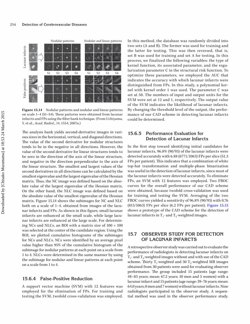
The analysis bank yields second-derivative images in vari-ous sizes in the horizontal, vertical, and diagonal directions. The value of the second derivative for nodular structures tends to be in the negative in all directions. However, the value of the second derivative for linear structures tends to be zero in the direction of the axis of the linear structure, and negative in the direction perpendicular to the axis of the linear structure. The smallest and largest values of the second derivatives in all directions can be calculated by the smallest eigenvalue and the largest eigenvalue of the Hessian matrix. Thus, the NC image was defined based on the abso-lute value of the largest eigenvalue of the Hessian matrix. On the other hand, the NLC image was defined based on the absolute value of the smallest eigenvalue of the Hessian matrix. Figure 15.14 shows the subimages for NC and NLC both on a scale of 1–4, obtained from images of the lacu-nar infarcts and FPs. As shown in this figure, small lacunar infarcts are enhanced at the small scale, while large lacu-nar infarcts are enhanced at the large scale. For determin-ing NCs and NLCs, an ROI with a matrix size of 100 × 100 was selected at the center of the candidate region. Using the ROI, we plotted cumulative histograms of the subimages for NCs and NLCs. NCs were identified by an average pixel value higher than 95% of the cumulative histogram of the subimage for nodular patterns at each point on a scale from 1 to 4. NLCs were determined in the same manner by using the subimage for nodular and linear patterns at each point on a scale from 1 to 4.
15.6.4 False-Positive Reduction
A support vector machine (SVM) with 12 features was employed for the elimination of FPs. For training and testing the SVM, twofold cross-validation was employed.
In this method, the database was randomly divided into two sets (A and B). The former was used for training and the latter for testing. This was then reversed, that is, set B was used for training and set A for testing. In this process, we finalized the following variables: the type of kernel function, its associated parameter, and the regu-larization parameter C in the structural risk function. To optimize these parameters, we employed the AUC that indicates the accuracy with which lacunar infarcts were distinguished from FPs. In this study, a polynomial ker-nel with kernel order 1 was used. The parameter C was set at 50. The numbers of input and output units for the SVM were set at 12 and 1, respectively. The output value of the SVM indicates the likelihood of lacunar infarcts. By changing the threshold level of the output, the perfor-mance of our CAD scheme in detecting lacunar infarcts could be determined.
15.6.5 Performance Evaluation for Detection of Lacunar Infarcts
In the first step toward identifying initial candidates for lacunar infarcts, 96.8% (90/93) of the lacunar infarcts were detected accurately with 6.88 (6771/1063) FPs per slice (51.3 FPs per patient). This indicates that a combination of white top-hat transformation and multiple-phase binarization was useful in the detection of lacunar infarcts, since most of the lacunar infarcts were detected accurately. To eliminate FPs, an SVM with 12 features was employed. Two FROC curves for the overall performance of our CAD scheme were obtained, because twofold cross-validation was used for training and testing the SVM. Averaging of the two FROC curves yielded a sensitivity of 96.8% (90/93) with 0.76 (813/1063) FPs per slice (6.2 FPs per patient). Figure 15.15 shows a prototype of the CAD scheme for the detection of lacunar infarcts in T1- and T2-weighted images.
15.7 OBSERVER STUDY FOR DETECTION OF LACUNAR INFARCTS
A retrospective observer study was carried out to evaluate the performance of radiologists in detecting lacunar infarcts on T1- and T2-weighted images without and with use of the CAD scheme. Thirty T1-weighted and 30 T2-weighted MR images obtained from 30 patients were used for evaluating observer performance. The group included 15 patients (age range: 48–83 years; mean: 67.2 years; 10 men and 5 women) with a lacunar infarct and 15 patients (age range: 39–76 years; mean: 64.0 years; 8 men and 7 women) without lacunar infarcts. Nine radiologists participated in the observer study. A sequen-tial method was used in the observer performance study.
Nodular patterns
S1 S2 S3 S4 S1 S2 S3 S4
Lacu
nar i
nfar
cts
False
pos
itive
s
Nodular and linear patterns
Figure 15.14 Nodular patterns and nodular and linear patterns on scale 1–4 (S1–S4). These patterns were obtained from lacunar infarcts and FPs using the filter bank technique. (From Uchiyama, Y. et al., Acad. Radiol., 14, 1554, 2007a.)
Dow
nloa
ded
by [
Chi
sako
Mur
amat
su]
at 1
8:53
24
Mar
ch 2
015

15.7 Observer Study for Detection of Lacunar Infarcts 255
T1- and T2-weighted images were displayed together at the same transverse location. The observers could manually control the speed or sequence of the slice image display, and they were allowed to change the window level and width on the monitor. Each observer reads all of the slice images for T1- and T2-weighted images displayed on the LCD monitor ini-tially without computer output. The observer marked his or her confidence level regarding the likelihood of the presence of a lacunar infarct. After the observer marked the initial level of confidence, the computer outputs were superimposed on the T1- and T2-weighted images. The observer again marked his or her confidence level if he or she wished to change the initial result.
The observers were given the following information: (a) The purpose of the study was to evaluate the perfor-mance of radiologists in detecting lacunar infarcts without and with the CAD scheme on T1- and T2-weighted images; (b) the role of the CAD output as a second opinion would be evaluated; (c) the observer study consisted of 30 MRI studies that did not or did contain a lacunar infarct and/or nonla-cunar lesions such as enlarged Virchow–Robin spaces; (d) the defined diameter of lacunar infarcts was 3–15 mm; (e) computer performance yielded a sensitivity of 96% and 0.76 FP per slice on average, and this result was not obtained from the 30 cases in this observer study; and (f) the observ-ers were instructed to click on the screen using a mouse (1) to indicate on a bar their confidence level regarding the presence (or absence) of a lacunar infarct and (2) to locate the most likely position in each case. Each observer used a continuous rating scale displayed on the monitor. The observers were blinded to the number of patients with a
lacunar infarct. The selected cases for the observer perfor-mance study were presented in the same randomized order to the observers. There was no limit on reading time.
ROC analysis was used for comparison between the radiol-ogists’ performances without and with the computer output for the detection of lacunar infarcts on T1- and T2-weighted images. Figure 15.16 shows ROC curves obtained from all
0.00.0
0.1
0.2
0.3
0.4
0.5
0.6
0.7
0.8
0.9
1.0
0.1 0.2 0.3 0.4 0.5False-positive fraction
p = 0.032
Without CAD (AUC = 0.891)
With CAD (AUC = 0.937)
True
-pos
itive
frac
tion
0.6 0.7 0.8 0.9 1.0
Figure 15.16 Average ROC curves obtained from nine radiolo-gists for the detection of lacunar infarcts without and with com-puter output. The average AUC value was significantly improved from 0.886 to 0.930 when observers used the computer output (p = 0.032).
Enlarged image
T1-weighted image T1-weighted image
Enlarged image
Figure 15.15 Illustration of a prototype CAD scheme for the detection of lacunar infarct.
Dow
nloa
ded
by [
Chi
sako
Mur
amat
su]
at 1
8:53
24
Mar
ch 2
015

Detection of Cerebrovascular Diseases256
the radiologists without and with the computer output. The average AUC values for all the radiologists improved from 0.891 (without the computer output) to 0.937 (with the computer output), and this difference was statistically sig-nificant (p = 0.032). Figure 15.17a shows clinically relevant changes in the confidence ratings of each observer with regard to patients with a lacunar infarct. The average num-ber of cases affected beneficially was 1.33 (8.9%). However, the average number of cases affected detrimentally was 0.33 (2.2%). In two out of the three detrimentally affected cases, the CAD scheme could not accurately detect the lacunar infarct. In one of the three detrimentally affected cases, the observers changed his/her confidence level into a lower value even though the CAD scheme accurately detected the lacu-nar infarct. Figure 15.17b shows clinically relevant changes in the confidence ratings of each observer with regard to patients without a lacunar infarct. The average number of cases affected beneficially and detrimentally were 3.67 (24.4%) and 0.89 (5.9%), respectively. The average number of patients without a lacunar infarct that were affected benefi-cially was higher than that of patients with a lacunar infarct. These beneficial effects were caused by the fact that observ-ers first marked lesions such as enlarged Virchow–Robin spaces with a relatively high confidence level indicating the presence of lacunar infarcts. However, the confidence level was changed to a lower value after taking into account the absence of lesions detected by CAD. Therefore, observers were able to make the correct diagnosis using the computer output. On the other hand, eight detrimentally affected cases were caused by FPs detected by the CAD scheme.
15.8 CLASSIFICATION OF LACUNAR INFARCTS AND ENLARGED VIRCHOW–ROBIN SPACES
In the observer study described earlier, we realized that the majority of FPs detected by the computer are differ-ent from those detected by radiologists, and radiologists
can therefore disregard these obvious FPs identified by the computer. However, it is of interest to note that some FPs due to enlarged Virchow–Robin spaces detected by the computer were difficult for radiologists to distinguish from lacunar infarcts. These FPs were the main sources to the detrimental effects of the CAD scheme. A strong influence on radiologists by these FPs might result in unnecessary medical treatment for the patient. Therefore, a CAD scheme for the classification of lacunar infarcts and enlarged Virchow–Robin spaces was developed to assist radiologists’ image interpretation (Uchiyama et al. 2008b).
15.8.1 Feature Extraction
The database consisted of T1- and T2-weighted images obtained from 109 patients, which included 89 lacunar infarcts and 20 enlarged Virchow–Robin spaces. These images were acquired using a 1.5 T MR scanner. The radiolo-gist selects regions of interest (ROIs) including a lesion. The morphological white top-hat transform was first employed for the enhancement of small focal hyperintensity lesions in ROIs of T2-weighted images. The gray-level thresholding technique was then employed for the segmentation of the lesions. To measure the characteristics of lacunar infarcts and enlarged Virchow–Robin spaces, six features were deter-mined from the segmented lesions. These features included the x and y coordinates, size, degree of irregularity, and signal intensity differences in T1- and T2-weighted images. The x and y coordinates were defined based on the centroid of the segmented region. Size was defined as the number of pixels in the segmented region. The degree of irregularity was given as 1-C/L, where C is the length of circumference of the circle having the same area as the segmented region, and L is the boundary length of the segmented region. The signal intensity differences in the T1- and T2-weighted images were defined as the difference between the average pixel value of the segmented region and the average pixel value of the peripheral region. Figure 15.18 shows the distribution of the six features obtained from 89 lacunar infarcts and
Num
ber o
f cas
es af
fect
edby
the c
ompu
ter o
utpu
t
A B C D EObservers
F G H I0
2
4
6
8
10BeneficialDetrimental
(a)
0Num
ber o
f cas
es af
fect
edby
the c
ompu
ter o
utpu
t
A B C D E
Observers
F G H I
2
4
6
8
10BeneficialDetrimental
(b)
Figure 15.17 Graphs showing the number of cases (>15%) affected by CAD output in confidence level with regard to patients (a) with a lacunar infarct and (b) without a lacunar infarct.
Dow
nloa
ded
by [
Chi
sako
Mur
amat
su]
at 1
8:53
24
Mar
ch 2
015

15.8 Classification of Lacunar Infarcts and Enlarged Virchow–Robin Spaces 257
20 enlarged Virchow–Robin spaces. Black and white circles indicate lacunar infarcts and enlarged Virchow–Robin spaces, respectively. Enlarged Virchow–Robin spaces are located at the central region on the right and left sides, as shown in Figure 15.18a. The sizes of enlarged Virchow–Robin spaces are relatively small comparable to those of lacunar infarcts, as shown in Figure 15.18b. Signal intensity differ-ences in T2-weighted image appear to be smaller for enlarged Virchow–Robin spaces than for lacunar infarcts, as shown in Figure 15.18c.
15.8.2 Classification Scheme
A neural network with six features was employed for distin-guishing between lacunar infarcts and enlarged Virchow–Robin spaces. A three-layer neural network, consisting of six input units, two hidden units, and one output unit, was used. The number of hidden units was determined empirically. The input data for the neural network were the six features determined in the previous section. The neural network
generates a decision boundary that optimally partitions the feature space into the two classes, that is, lacunar infarcts and enlarged Virchow–Robin spaces. The output value of the neural network indicates the likelihood of occurrence of the lacunar infarct. For training and testing of the neural network, the leave-one-out method was employed. To evalu-ate the classification performance, ROC analysis was used; the AUC value was 0.945. The sensitivity and specificity of detection of lacunar infarcts were 93.3% (83/89) and 75.0% (15/20), respectively. The results indicate that this comput-erized method may be useful for the classification of lacu-nar infarcts and enlarged Virchow–Robin spaces in T1- and T2-weighted images.
15.8.3 Fusion Image of T2-Weighted Image and MRA
MRA images acquired with 3 T MR scanner can visualize blood flow inside small vessels. Therefore, a fusion image of a T2-weighed image and an MRA may be useful for distinction
100100
200
300
400
200x Coordinate
y Coo
rdin
ate
300 400(a) (b)
00.0
0.1
0.2
0.3
0.4
0.5
0.6
50 100 150Size (number of pixels)
Deg
ree o
f irr
egul
arity
200 250 300 350
–2000
50
100
150
200
250
300
350
400
450
–150 –100Signal intensity di�erence in T1-WI
Sign
al in
tens
ity d
i�er
ence
in T
2-W
I
–50 0 50(c)
Figure 15.18 Distribution of six features obtained from lacunar infarcts and enlarged Virchow–Robin spaces. (a) Relation between x and y coordinates. (b) Relationship between size and degree of irregularity. (c) Relationship between signal intensity difference in T1-weighted image (WI) and signal intensity difference in T2-weighted image (WI). (From Uchiyama, Y. et al., Conf. Proc. IEEE Eng. Med. Biol., 3908, 2008b.)
Dow
nloa
ded
by [
Chi
sako
Mur
amat
su]
at 1
8:53
24
Mar
ch 2
015

Detection of Cerebrovascular Diseases258
between lacunar infarcts and enlarged Virchow–Robin spaces (Uchiyama et al. 2009). Because enlarged Virchow–Robin spaces are formed by atrophy of the tissue surround-ing a cerebral artery, blood flow inside the small artery can be observed in these images. However, in the case of lacu-nar infarct, blood flow is absent. Figure 15.19 illustrates a fusion image of a T2-weighed image and an MRA, which were acquired with a 3 T MR scanner. In the fusion image, blood flow is clearly visible in the lesion, facilitating the identification of the lesion as an enlarged Virchow–Robin
space. To enerate the fusion image, we determined the location of 2D T2-weighted images in the 3D MRA image using an image registration technique. In this method, a similarity measure was employed based on the pixel values of the T2-weighted image and the voxel values of the slice image along the body axis of the 3D MRA image. The vessel regions in MRA image were segmented using the threshold-ing and region-growing techniques, described in Section 15.2.1. Volume rendering was then used to generate the fusion image.
(a) (b)
(c)
Figure 15.19 Illustration of fusion image of T2-weighted image and MRA. (a) T2-weighted image. (b) Fusion image in the bottom-to-top direction. (c) Fusion image in the top-to-bottom direction. (From Uchiyama, Y. et al., IFMBE Proc., 126, 2009.)
Dow
nloa
ded
by [
Chi
sako
Mur
amat
su]
at 1
8:53
24
Mar
ch 2
015

259References
15.9 CONCLUSIONS
A number of CAD schemes have been developed for the detec-tion and/or classification of cerebrovascular diseases. Observer performance studies indicated that computer output helps radiologists improve their diagnostic accuracy. Therefore, CAD schemes will be useful in assisting radiologists in their assessment of cerebrovascular diseases on MR images.
REFERENCESArimura, H., Q. Li, Y. Korogi, T. Hirai, H. Abe, Y. Yamashita et al. 2004.
Automated computerized scheme for detection of unrup-tured intracranial aneurysms in three-dimensional MRA. Academic Radiology 11:1093–1104.
Arimura, H., Q. Li, Y. Korogi, T. Hirai, S. Katsuragawa, Y. Yamashita et al. 2006. Computerized detection of intracranial aneurysms for three-dimensional MR angiography: Feature extraction of small protrusions based on a shape-based difference image technique. Medical Physics 33:394–401.
Bokura, H., S. Kobayashi, and S. Yamaguchi. 1998. Discrimination of silent lacunar infarction from enlarged Virchow-Robin spaces on brain magnetic resonance imaging: Clinicopathological study. Journal of Neurology 245:116–122.
Fogelholm, R., J. Hernesniemi, and M. Vapalahti. 1993. Impact of early surgery on outcome after aneurysm subarachnoid hem-orrhage: A population-based study. Stroke 24:1649–1654.
Fujita, H., Y. Uchiyama, T. Nakagawa, D. Fukuoka, Y. Hatanaka, T. Hara et al. 2008. Computer-aided diagnosis: The emerging of three CAD systems induced by Japanese health care needs. Computer Methods and Programs in Biomedicine, Review, 92(3):238–248.
Gao, X., Y. Uchiyama, X. Zhou, T. Hara, T. Asano, and H. Fujita. 2011. A fast and fully automatic method for cerebrovascular seg-mentation on time-of-flight (TOF) MRA image. Journal of Digital Imaging 24(4):609–625.
Hayashi, H., Y. Masutani, T. Matsumoto, H. Mori, A. Kunimatsu, O. Abe et al. 2003. Feasibility of a curvature-based enhanced display system for detecting cerebral aneurysms in MR angi-ography. Magnetic Resonance in Medical Science 2:29–36.
Hirai, T., Y. Korogi, H. Arimura, S. Katsuragawa, M. Kitajima, M. Yamura et al. 2006. Intracranial aneurysms at MR angi-ography: Effect of computer-aided diagnosis on radiologists’ detection performance. Radiology 237:605–610.
Kakeda, S., Y. Korogi, H. Arimura, T. Hirai, S. Katsuragawa, T. Aoki et al. 2008. Diagnostic accuracy and reading time to detect intracranial aneurysms on MR angiography using a com-puter-aided diagnosis system. AJR 190:459–465.
Kobayashi, S., K. Kondo, and Y. Hata. 2006. Computer-aided diagno-sis of intracranial aneurysms in MRA images with case-based reasoning. IEICE Transactions on Information and Systems E89-D(1):340–350.
Kobayashi, S., K. Okada, H. Koide, H. Bokura, and S. Yamaguchi. 1997. Subcortical silent brain infarction as a risk factor for clinical stroke. Stroke 28:1932–1939.
Li, Q., S. Sone, and K. Doi. 2003. Selective enhancement filters for nodule, vessels, and airway walls in two- and three dimen-sional CT scan. Medical Physics 30:2040–2051.
Nakayama, R., Y. Uchiyama, K. Yamamoto, R. Watanabe, and K. Namba. 2006. Computer-aided diagnosis scheme using a filter bank for detection of microcalcification clusters in mammograms. IEEE Transactions on Biomedical Engineering 53:273–283.
Shintani, S., T. Shiigai, and T. Arinami. 1998. Silent lacunar infarc-tion on magnetic resonance imaging (MRI): Risk factors. Journal of Neurological Science 160:82–86.
Uchiyama, Y., H. Ando, R. Yokoyama, T. Hara, H. Fujita, and T. Iwama. 2005. Computer-aided diagnosis scheme for detec-tion of unruptured intracranial aneurysms in MR angiogra-phy. Conference of Proceedings of IEEE Engineering in Medicine and Biology, Shanghai, IEEE, 2005:3031–3034.
Uchiyama, Y., T. Asano, T. Hara, H. Fujita, H. Hoshi, T. Iwama et al. 2009. CAD Scheme for differential diagnosis of lacu-nar infarcts and normal Virchow-Robin spaces on brain MR images. IFMBE Proceedings, Munich, Springer, 126–128.
Uchiyama, Y., X. Gao, T. Hara, H. Fujita, H. Ando, H. Yamakawa et al. 2008a. Computerized detection of unruptured aneurysms in MRA images: Reduction of false posi-tives using anatomical location feature. SPIE Proceedings 6915: 69151Q-1–69151Q-8.
Uchiyama, Y., T. Kunieda, T. Asano, H. Kato, T. Hara, M. Kanematsu et al. 2008b. Computer-aided diagnosis scheme for classifica-tion of lacunar infarcts and enlarged Virchow-Robin spaces in brain MR image. Conference of Proceedings of IEEE Engineering in Medicine and Biology, Vancouver, IEEE, 3908–3911.
Uchiyama, Y., M. Yamauchi, H. Ando, R. Yokoyama, T. Hara, H. Fujita et al. 2006. Automated classification of cerebral arteries in MRA images and its application to maximum intensity projection. Conference Proceedings of IEEE Engineering in Medicine and Biology, New York, IEEE, 4865–4868.
Uchiyama, Y., R. Yokoyama, H. Ando, T. Asano, H. Kato, H. Yamakawa et al. 2007a. Computer-aided diagnosis scheme for detec-tion of lacunar infarcts on MR image. Academic Radiology 14:1554–1561.
Uchiyama, Y., R. Yokoyama, T. Asano, H. Kato, H. Yamakawa, H. Ando et al. 2007b. Improvement of automated detection method of lacunar infarcts in brain MR images. Conference Proceedings of IEEE Engineering in Medicine and Biology, Lyon, IEEE, 1599–1602.
Vermeer, S.E., M. Hollander, E. J. Dijk, A. Hofman, P. J. Koudstaal, and M. M. Breteler. 2003. Silent brain infarcts and white mat-ter lesions increase stroke risk in the general population: The Rotterdam scan study. Stroke 34:1126–1129.
Wardlaw, J. M., P. M. White. 2000. The detection and management of unruptured intracranial aneurysms. Brain 123:205–221.
Yamauchi, M., Y. Uchiyama, R. Yokoyama, T. Hara, H. Fujita, H. Ando et al. 2007. Computerized scheme for detection of arterial obstruction in brain MRA images. SPIE Proceedings 6514:65142C-1–65142C-9.
Yang, X., DJ. Blezek, LT. Cheng, WJ. Ryan, DF. Kallmes, and BJ Erickson. 2011. Computer-aided detection of intracranial aneurysms in MR angiography. Journal of Digital Imaging 24:86–95.
Yokoyama, R., X. Zhang, Y. Uchiyama, H. Fujita, T. Hara, X. Zhou et al. 2007. Development of an automated method for detection of chronic lacunar infarct regions on brain MR images. IEICE Transactions on Information and Systems E90-D(6):943–954.
Dow
nloa
ded
by [
Chi
sako
Mur
amat
su]
at 1
8:53
24
Mar
ch 2
015

Dow
nloa
ded
by [
Chi
sako
Mur
amat
su]
at 1
8:53
24
Mar
ch 2
015