Detection and Measurement of Radar Signals: A Tutorial

7th Annual ISART

Frank H. Sanders

NTIA Institute for Telecommunication Sciences

1 March 2005

OUTLINE

1. RADAR EMISSION FUNDAMENTALS a) Pulse duty cycles

b) Transmitter peak power levels

c) Antenna gain

d) US radar spectrum bands

2. RADAR PARAMETERS

a) Radar spectrum engineering criteria (RSEC)

b) Waveform (pulse) width, rise time, fall time,

modulation

c) Pulse repetition rate

d) Antenna patterns

e) Emission spectra

a. Measurement hardware and algorithms

b. Measurement dependence on bandwidth

c. Do spectra have to be measured in the far

field?

2

RADAR EMISSION FUNDAMENTALS

-Emissions are pulsed. Usually about 0.1% duty

cycle (typically 1 us pulse width, and 1 ms pulse

repetition interval).

-Peak transmitter power levels often around 1 MW.

-Antenna gain often around 30 dBi.

-Peak EIRP levels around 1 GW.

Mission Pulse width

(us)

Pulse rate

(Hz)

Peak power (MW)

An-tenna gain (dBi)

PeakEIRP

(GW) Short range air search

1 1000 0.8 33 1.6

Long range air search

3-10 300 1 33 2

Maritime navigation

0.08-0.8 10000 0.02 30 0.02

Weather 1-5 300-1300

0.75 45 24

3

MAJOR US RADAR SPECTRUM BANDS

5-25 MHz HF OTH-B functions 420-450 MHz space search, airborne search 902-928 MHz air search 1215-1400 MHz long range air search 2700-2900 MHz air traffic control (terminals) 2900-3100 MHz air & marine search, weather 3100-3700 MHz air search 5250-5925 MHz air search, weather 8.5-10.5 GHz airborne functions 13.4-14.0 GHz airborne functions 15.7-17.7 GHz airborne functions 24.05-24.25 GHz low power (e.g., police radars)

4

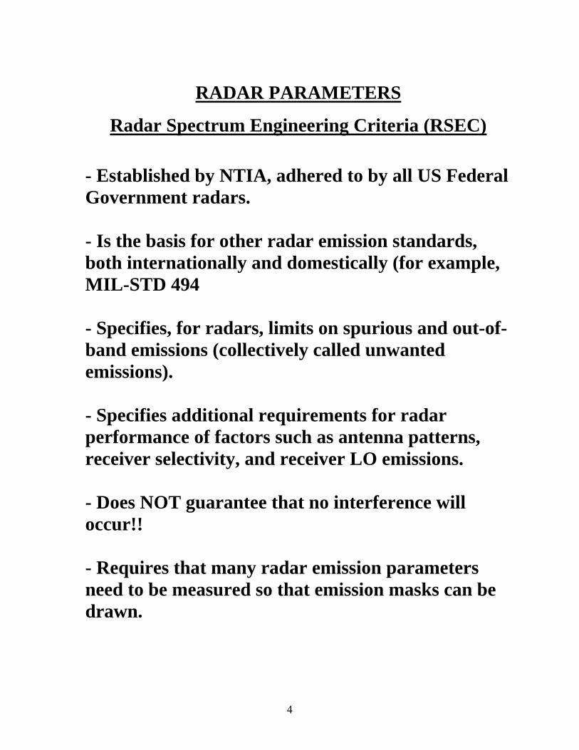
RADAR PARAMETERS

Radar Spectrum Engineering Criteria (RSEC)

- Established by NTIA, adhered to by all US Federal Government radars. - Is the basis for other radar emission standards, both internationally and domestically (for example, MIL-STD 494 - Specifies, for radars, limits on spurious and out-of-band emissions (collectively called unwanted emissions). - Specifies additional requirements for radar performance of factors such as antenna patterns, receiver selectivity, and receiver LO emissions. - Does NOT guarantee that no interference will occur!! - Requires that many radar emission parameters need to be measured so that emission masks can be drawn.

5

- Does not explain how to do the measurements—See NTIA Reports and ITU-R Recommendation M.1177 for such explanations.

6

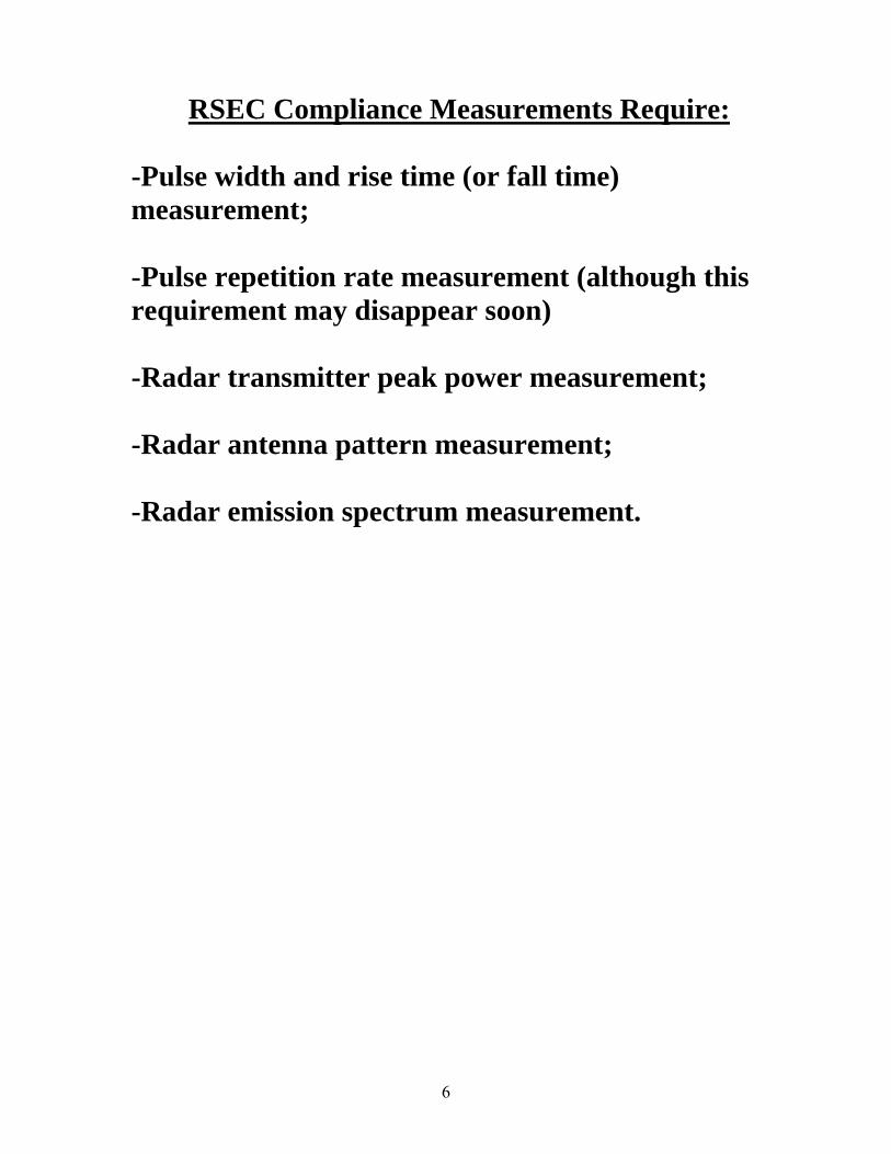
RSEC Compliance Measurements Require:

-Pulse width and rise time (or fall time) measurement; -Pulse repetition rate measurement (although this requirement may disappear soon) -Radar transmitter peak power measurement; -Radar antenna pattern measurement; -Radar emission spectrum measurement.

7

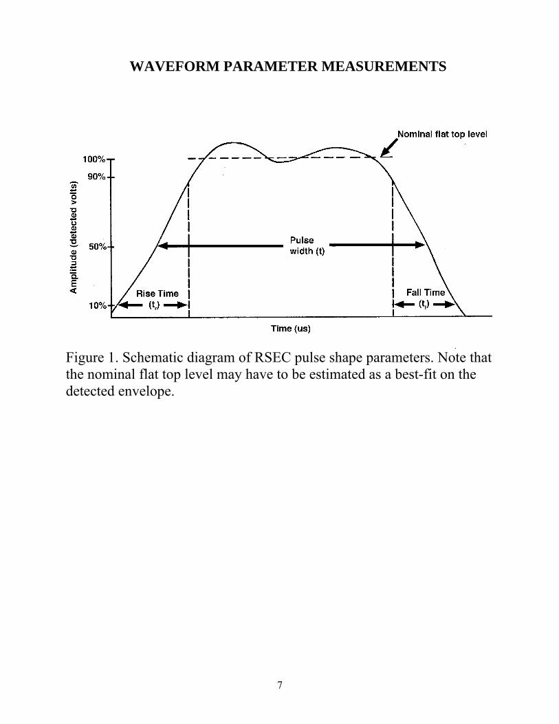
WAVEFORM PARAMETER MEASUREMENTS

Figure 1. Schematic diagram of RSEC pulse shape parameters. Note that the nominal flat top level may have to be estimated as a best-fit on the detected envelope.

8

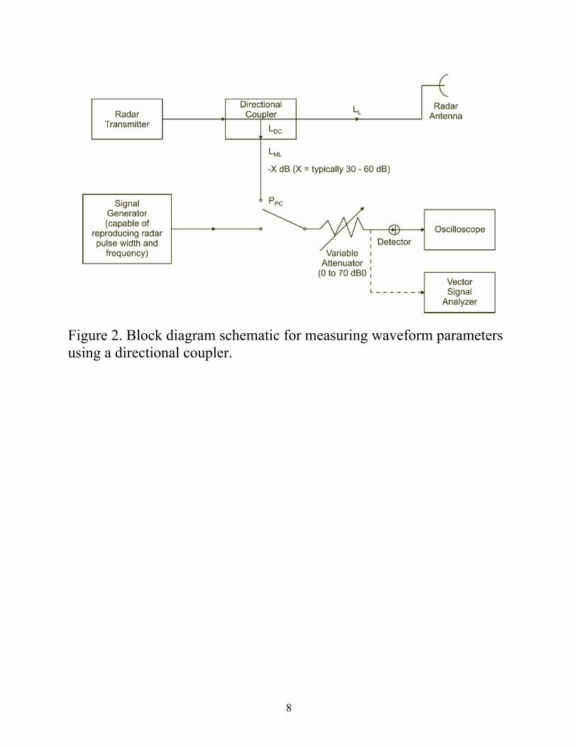
Figure 2. Block diagram schematic for measuring waveform parameters using a directional coupler.

9

Figure 3. Block diagram schematic for measuring radiated waveform.

10

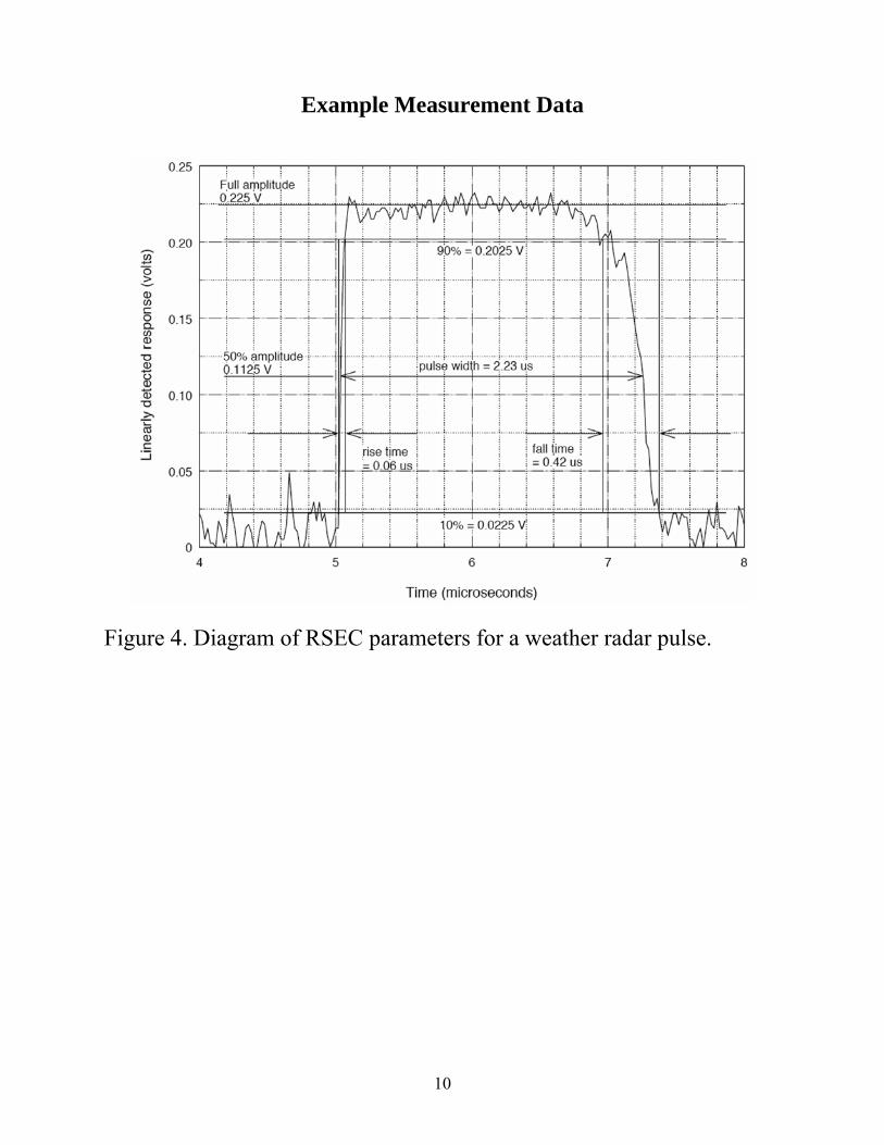
Example Measurement Data

Figure 4. Diagram of RSEC parameters for a weather radar pulse.

11

Figure 5. Diagram of RSEC parameters for a short-range search radar pulse.

12

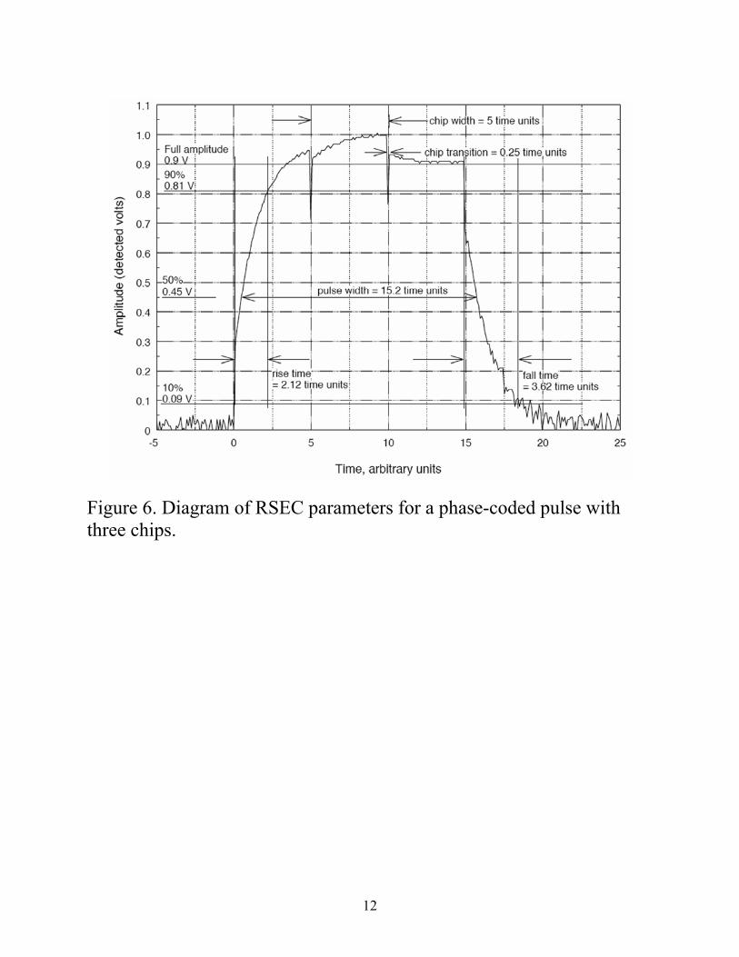
Figure 6. Diagram of RSEC parameters for a phase-coded pulse with three chips.

13

Figure 7. Measurement of the frequency deviation in time of a frequency-modulated pulse.

14

2. PULSE REPETITION RATE

Example Measurement Data

0.15

0.20

0.25

0.30

0.35

0.40

0 1 2 3 4 5 6 7 8 9 10

-1pulse repetition rate = 1096 sec

pulse repetition interval = 0.913 mS

Time (milliseconds)

Am

plitu

de (

dete

cted

vol

ts)

Figure 8. Example of a fixed-PRR radar pulse sequence.

15

Figure 9. Pulse repetition measurement on a single channel of a frequency-hopping radar made with a spectrum analyzer in a zero-Hertz span mode and positive peak detection. The line is an estimated threshold for on-frequency pulses.

16

0

0.04

0.08

0.12

0 0.5 1.0 1.5 2.0

Time (msec)

Am

plitu

de (

dete

cted

vol

ts)

Figure 10. The pulse repetition rate of the same radar as that shown in Figure 9, but measured with a broadband detector configured as in Figure 3.

17

5. EMISSION SPECTRA Table 1. Determination of RSEC Measurement Bandwidth (Bm) Radar Modulation Type RSEC Measurement Bandwidth (Bm): Non-FM pulsed and phase-coded pulsed

Bm ≤ (1/t), where t = emitted pulse duration (50% voltage) or phase-chip (sub-pulse) duration (50% voltage). Example for non-FM pulsed: If emitted pulse duration is 1 µs, then Bm ≤ 1 MHz. Example for phase-coded pulsed: If radar transmits 26-µs duration pulses, each pulse consisting of 13 phase-coded chips that are each 2µs in duration, then Bm ≤ 500 kHz.

FM-pulsed (chirped) Bm ≤ (Bc/t)1/2, where Bc = frequency sweep range during each pulse and t = emitted pulse duration (50% voltage). Example: If radar sweeps (chirps) across frequency range of 1.3 MHz during each pulse, and if the pulse duration is 55 μs, then Bm ≤ 154 kHz.

CW Bm = 1 kHz; See sub-paragraph 4.2 of [1, Chapter 5] for RSEC Criteria B, C and D. Example: Bm = 1 kHz.

FM/CW Bm = 1 kHz; See sub-paragraph 4.2 of [1, Chapter 5] for RSEC Criteria B, C and D.

Example: Bm = 1 kHz Phase-coded CW Bm ≤ (1/t), where t = emitted phase-chip duration (50% voltage).

Example for phase-coded pulsed: If chip duration is 2µs, then Bm ≤ 500 kHz.

Multi-mode radars Calculations should be made for each waveform type as described above, and the minimum resulting value of Bm should be used for the emission spectrum measurement. Example: A multi-mode radar produces a mixture of pulse modulations as used in the above examples for non-FM pulsed and FM-pulsed. These values are 1 MHz and 154 kHz, respectively. Then Bm ≤ 154 kHz.

18

-70

-60

-50

-40

-30

-20

-10

0

10

20

30

40

50

0 10 20 30 40

1 kHz

3 kHz

10 kHz

30 kHz

100 kHz300 kHz1 MHz3 MHz

Arbitrary Units

Rec

eive

d P

ower

in In

dica

ted

Ban

dwid

th (

dBm

)

Figure 11. Example of a bandwidth progression measurement for assessment of the proper bandwidth in which to measure a radar spectrum for RSEC compliance.

19

-90

-80

-70

-60

-50

-40

-30

-20

-10

0

10

2700 2750 2800 2850 2900

300 kHz100 kHz

Frequency (MHz)

Mea

sure

d P

ower

Lev

el in

Spe

cifie

d B

andw

idth

(dB

m)

Figure 12. Emission spectrum measurement performed on a multi-mode chirped radar.

20

Figure 13. An example of a spectrum measurement error caused by an incorrect RF attenuation setting.

21

Figure 14. Example spectrum of an air search radar.

22

Figure 15. Example bandwidth progression measurement of the fundamental for the radar having the measured emission spectra of Figure 16.

23

Figure 16. Three spectra for a single radar for which the bandwidth progression is shown in Figure 15.

24

4. ANTENNA PATTERNS .

Figure 17. Example radar antenna pattern for a surface search radar.

25

Figure 18. Three antenna patterns (top) & median of patterns (bottom).

26

APPENDIX A: DEFINITIONS

A.1 Spectrum Regions

Table A-1. Definitions of Spectrum Regions and Related Terms, from Chapter 6 of [1]

Term Definition Necessary bandwidth

For a given class of emission, the width of the frequency band which is just sufficient to ensure the transmission of information at the rate and with the quality required under specified conditions. Necessary bandwidths for radars as a function of emission type are provided in Annex J of [1].

Out-of-band emissions

Emission on a frequency or frequencies immediately outside the necessary bandwidth which results from the modulation process, but excluding spurious emission.

Spurious emissions

Emission on a frequency or frequencies which are outside the necessary bandwidth and the level of which may be reduced without affecting the corresponding transmission of information. Spurious emissions include harmonic emissions, parasitic emissions, intermodulation products and frequency conversion products, but exclude out-of-band emissions.

Unwanted emissions

These consist of spurious emissions and out-of-band emissions.

27

APPENDIX B: ENSURING ADEQUATE MEASUREMENT SYSTEM INPUT ATTENUATION FOR RSEC

MEASUREMENTS

B.1 Hardline Coupling to a Radar Transmitter For hardline-coupled measurements, some attenuation will likely be required between the directional coupler output and the measurement device input (see Figure 1). Referring to this diagram, the minimum decibel amount of attenuation, A, required will be:

(B-1) where Aext = external attenuation (dB) as shown in Figure 1 Pp = peak power produced by the radar transmitter (dBm) Lc = loss through the coupler (dB) Ain = attenuation provided internally at the measurement device front end input (dB) Pm = maximum input power to measurement instrument after input attenuator (dBm). For example, if the radar transmitter produces 1 MW (+90 dBm) peak power, if the directional coupler output is 20 dB lower than that value, and if the maximum permissible signal allowed at the spectrum analyzer input is +10 dBm with 50 dB of internal spectrum analyzer attenuation invoked at the front end, then the amount of attenuation that needs to be inserted between the coupler output and the spectrum analyzer input is

(90–20–50–10) = 10 dB. In this case, even with 50 dB of RF attenuation invoked in the instrument’s front end, an additional 10 dB of external RF attenuation is required between the directional coupler and the measurement device input.

B.2 Radiated Coupling to a Radar Transmitter All the caveats regarding maximum allowable input power levels and optimal linear response and calibration range for measurement instrumentation, as described in section B.1 above, also apply to the case of radiative coupling between the measurement system and the radar transmitter. Here, the external attenuation, Aext, is inserted between the measurement antenna output connector and the measurement device (e.g., spectrum analyzer) input port. The difference is that the term for peak power at the measurement system antenna output connector, Pr, is (from Appendix C of [3]):

mincpext PALPA −−−=

28

minrext PAPA −−=

(B-2) where Pr = peak power at the measurement system antenna output connector (dBm); Pp = peak power produced by the radar transmitter (dBm); Gt = radar transmitter antenna gain (dBi); Gr = measurement system antenna gain (dBi); f = measurement frequency (MHz); r = distance between radar antenna and measurement antenna (meters). The variable Pr takes the place of Pp in Eq. B-1, and the value for the external attenuation, Aext, becomes:

(B-3) where all variables are as defined for Eq. B-1. For example, suppose a radar transmitter operates at 2800 MHz; that the transmitter produces 1 MW peak power (+90 dBm); that the transmitter antenna gain is +35 dBi; that the measurement system antenna gain is +25 dBi; that the measurement system is positioned 0.5 miles (0.8 km, or 800 m) from the radar; that the maximum allowable peak power to be coupled into the measurement system is +30 dBm; and that 50 dB of RF attenuation is to be invoked within the measurement instrument RF front end. Then from Eq. B-2,

Pr = 90+35+25+27.6–20log(2800)–20log(800) = +50.6 dBm And from Eq. B-3,

Aext = 50–50–30 = –30 dB. The negative sign in the answer means that the signal coupled past the measurement instrument RF front end will actually be 30 dB below the maximum allowable limit of +30 dBm for this situation. No external attenuation is needed in this case. On the other hand, if the goal is to limit the peak power level that couples into the measurement instrument beyond its own RF front end attenuation to a value of –20 dBm or less, then

Aext = 50–50–(–20) = 20 dB. So in this case 20 dB of external attenuation would need to be inserted between the measurement antenna output connector and the input port of the measurement device.

( ) ( )rfGGPP rtpr log20log206.27 −−+++=

29

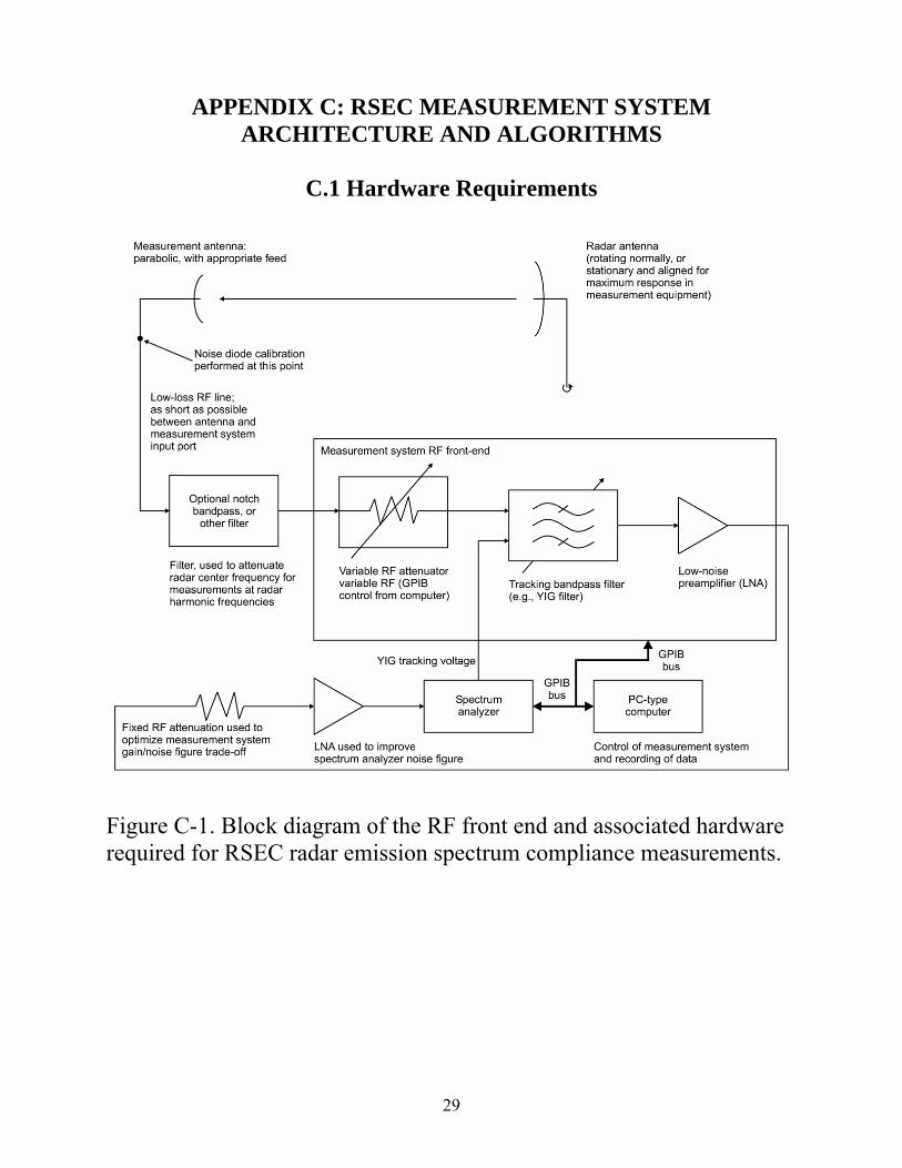
APPENDIX C: RSEC MEASUREMENT SYSTEM ARCHITECTURE AND ALGORITHMS

C.1 Hardware Requirements

Figure C-1. Block diagram of the RF front end and associated hardware required for RSEC radar emission spectrum compliance measurements.

30

Figure C-2. Block diagram of the RF front end and associated hardware required for RSEC radar emission spectrum compliance measurements on high frequency (HF) radars operating below about 50 MHz.

31

Figure C-4. RSEC measurement procedure flowchart.

32

Table C-1. Measurement System Parameters for Determination of Radar Fundamental Frequency or Frequencies

Measurement system parameter

Parameter setting

IF bandwidth 1 MHz Video bandwidth Equal to or greater than 1 MHz Detection mode Positive peak Frequency sweep range Operational band of the radar Frequency sweep rate Maximum allowed for the combination

of measurement bandwidth and frequency sweep range

Trace display mode Maximum hold Front end attenuation Sufficient to prevent measurement

system overload (adjusted empirically)

33

Figure C-4. Diagram of out-of-band and spurious emission suppression levels required by the RSEC. It should be noted that Recommendation ITU-R SM.329 recommends under category B more stringent limits than those given within Appendix S3 in some cases. This should be taken into account when evaluating the required range of measurement and the recommended dynamic range of the measurement system.

34

APPENDIX D: MEASUREMENT SYSTEM CALIBRATION

Figure D-1. Lumped component diagram of noise diode calibration.

Noise factor is the ratio of noise power from a device, ndevice(W), and thermal noise,

kTBndevice where k is Boltzmann’s constant (1.38·10−23J/K), T

is system temperature in Kelvin, and B is bandwidth in hertz. The excess noise ratio is equal to the noise factor minus one, making it the fraction of power in excess of kTB. The noise figure of a system is defined as 10 log (noise factor). As many noise sources are specified in terms of excess noise ratio, that quantity may be used.

35

( ) gkTBenrnfp dson ×+=

In noise diode calibration, the primary concern is the difference in output signal when the noise diode is switched on and off. For the noise diode = on condition, the power, Pon(W), is given by:

(D-1)

where nfs is system noise factor and enrd is the noise diode enr.

When the noise diode is off, the power, Poff(W), is given by:

poff = nfs( )× gkTB (D-2)

The ratio between Pon and Poff is the Y factor:

y =pon

poff

⎛

⎝ ⎜ ⎜

⎞

⎠ ⎟ ⎟ =

nfs + enrd( )nfs

(D-3)

Y =10log(y) =10log pon

poff

⎛

⎝ ⎜ ⎜

⎞

⎠ ⎟ ⎟ = Pon − Poff

Hence the measurement system noise factor can be solved as:

1−=

yenrnf d

s (D-4)

The measurement system noise figure is:

NFs =10log enrd

y −1⎛

⎝ ⎜

⎞

⎠ ⎟ = ENRd −10log y −1( )= ENRd −10log 10Y /10 −1( ) (D-5)

Hence:

g =pon − poff

enrd × kTB (D-6)

G =10log pon − poff( )−10log enrd × kTB( )

or

G =10log 10Pon /10 −10Poff /10( )− ENRd −10log kTB( )

In noise diode calibrations, the preceding equation is used to calculate measurement system gain from measured noise diode values.

36

Although the equation for NFs may be used to calculate the measurement system noise figure, software may implement an equivalent equation:

gkTBp

nf offs = (D-7)

( ) ( ) ( )kTBGPgkTBpNF offoffs log10log10log10 −−=−=

And substituting the expression for gain into the preceding equation yields:

( )10/10/ 1010log10 offon PPdoffs ENRPNF −−+= (D-8)

37

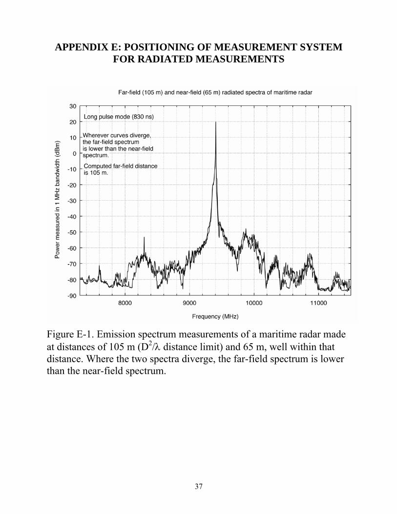
APPENDIX E: POSITIONING OF MEASUREMENT SYSTEM FOR RADIATED MEASUREMENTS

Figure E-1. Emission spectrum measurements of a maritime radar made at distances of 105 m (D2/λ distance limit) and 65 m, well within that distance. Where the two spectra diverge, the far-field spectrum is lower than the near-field spectrum.

38

APPENDIX F: VARIATION IN MEASURED PULSE SHAPES ACROSS EXTENDED EMISSION SPECTRA

(a) (b)

(c) (d)

Figure F-1. A weather radar pulse envelope measured at nominal radar center frequency (a), and at three other frequencies in the out-of-band and spurious parts of the emission spectrum ((b) through (d)). Measurement bandwidth was 8 MHz. The emission lines convolved at the center frequency in the measurement bandwidth yield a good approximation of the full-bandwidth pulse envelope in the time domain. But the subsets of Fourier lines convolved in the same bandwidth at frequencies in the out-of-band spurious portions of the emission spectrum do not yield the nominal pulse envelope; instead they tend to produce high-amplitude features in the leading edge, trailing edge, or both.

39

APPENDIX G: VARIATION IN MEASURED SPURIOUS AMPLITUDES AS A FUNCTION OF MEASUREMENT

BANDWIDTH

Figure G-1. Maritime radar and measurement system.

40

Figure G-2. Measurement system functional block diagram.

41

Figure G-3. Maritime radar emission spectrum measured in four bandwidths with transmitter operating in short-pulse mode.

42

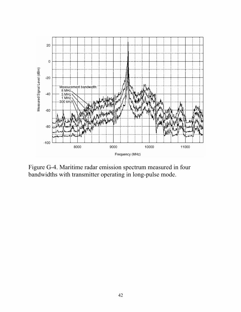
Figure G-4. Maritime radar emission spectrum measured in four bandwidths with transmitter operating in long-pulse mode.

43

Figure G-5. Variation in measured power at the radar fundamental as a function of measurement bandwidth and pulse mode. .

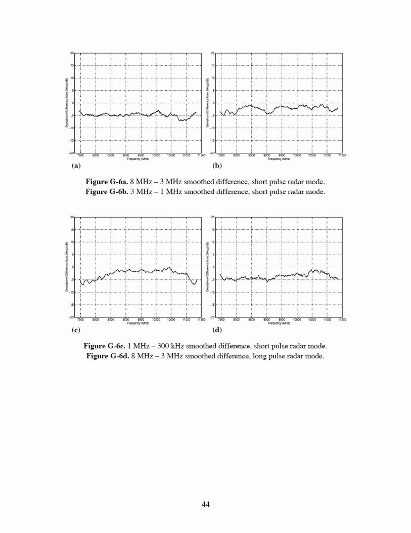
44

45