Detecting Urban Black Holes Based on Human MobilityData

Liang Hong 1, Yu Zheng 2∗, Duncan Yung 3, Jingbo Shang 4, Lei Zou 5

1Wuhan University, Wuhan, China, hong@whu.edu.cn2Microsoft Research, Beijing, China; Shanghai Jiao Tong University, Shanghai, China, yuzheng@microsoft.com

3University of Pittsburgh, USA, duncanyung@cs.pitt.edu4Shanghai Jiao Tong University, Shanghai, China, shangjingbo@apex.sjtu.edu.cn

5Peking University, Beijing, China; Key Laboratory of Computational Linguistics (PKU), Ministry of Education, China, zoulei@pku.edu.cn

ABSTRACTMany types of human mobility data, such as flows of taxicabs, cardswiping data of subways, bike trip data and Call Details Records(CDR), can be modeled by a Spatio-Temporal Graph (STG). STGis a directed graph in which vertices and edges are associated withspatio-temporal properties (e.g. the traffic flow on a road and thegeospatial location of an intersection). In this paper, we instant-ly detect interesting phenomena, entitled black holes and volcanos,from an STG. Specifically, a black hole is a subgraph (of an STG)that has the overall inflow greater than the overall outflow by athreshold, while a volcano is a subgraph with the overall outflowgreater than the overall inflow by a threshold (detecting volcanosfrom an STG is proved to be equivalent to the detection of blackholes). The online detection of black holes/volcanos can time-ly reflect anomalous events, such as disasters, catastrophic acci-dents, and therefore help keep public safety. The patterns of blackholes/volcanos and the relations between them reveal human mo-bility patterns in a city, thus help formulate a better city planning orimprove a system’s operation efficiency. Based on a well-designedSTG index, we propose a two-step black hole detection algorithm:The first step identifies a set of candidate grid cells to start from;the second step expands an initial edge in a candidate cell to a blackhole and prunes other candidate cells after a black hole is detect-ed. Then, we adapt this detection algorithm to a continuous blackhole detection scenario. We evaluate our method based on Bei-jing taxicab data and the bike trip data in New York, finding urbananomalies and human mobility patterns.

Categories and Subject DescriptorsH.2.8 [Database Management]: Database Applications-data min-ing, Spatial Databases and GIS

KeywordsUrban computing, Spatio-temporal graph, Black hole detection

1. INTRODUCTIONAdvances in sensing technology have lead to a huge amount of

human mobility data [24], such as flows of taxicabs, card swipingdata of subways, bike trip data and Call Details Records (CDR),

∗Yu Zheng is the correspondence authorPermission to make digital or hard copies of all or part of this work for personal orclassroom use is granted without fee provided that copies are not made or distributedfor profit or commercial advantage and that copies bear this notice and the full citationon the first page. Copyrights for components of this work owned by others than theauthor(s) must be honored. Abstracting with credit is permitted. To copy otherwise, orrepublish, to post on servers or to redistribute to lists, requires prior specific permissionand/or a fee. Request permissions from Permissions@acm.org.SIGSPATIAL ’15 November 03 - 06 2015, Bellevue, WA, USAc©2015 ACM ISBN 978-1-4503-3967-4/15/11 ...$15.00.

DOI: http://dx.doi.org/10.1145/2578726.2578744.

which can be modeled by a Spatio-Temporal Graph. A Spatio-Temporal Graph (STG) is a directed graph in which vertices andedges have geospatial positions and spatial lengths respectively,and are associated with spatio-temporal attributes. For example,as shown in Fig. 1(a), in a road network, POIs (Point Of Interests)with geographical positions can be regarded as vertices, and roadsegments between POIs can be modeled as edges. Traffic flows be-tween POIs always change dynamically over time, and edges canbe removed from the graph due to a traffic control or a disaster.Likewise, the bike sharing system illustrated in Fig. 1(b) can bemodeled as an STG, where bike stations can be regarded as ver-tices and the connections between them as edges. The cycling usersform the traffic flows between bike stations.

In an STG, we can find interesting phenomena, e.g. black holesand volcanos, which may represent urban anomalies or people’sregular travel patterns. Specifically, a black hole is a subgraph ofan STG that has the overall inflow greater than the overall outflowby a threshold, while a volcano is such a subgraph that has theoverall outflow greater than the overall inflow by a threshold. Asdifferent applications usually have different spatial constraint on ablack hole or volcano(e.g. what if an entire city is a black hole in abike sharing system), a spatial threshold on the size of a black holeis usually needed during the detection.

Black hole /Volcano Traffic Flow

A

B

(a) Stampede in Shanghai (b) NYC Bike Sharing System

e1

5

2

e2

3

4

2e3e4

D

E

C

Figure 1: Two Examples of Black Holes and VolcanosExample 1: As illustrated in Fig. 1(a), based on taxicab data and

CDR data, when the 2015 new year countdown in Shanghai was ap-proaching, the majority of people started to leave the bar street tothe Bund, forming a volcano A; 1 hour later many of them will en-ter a firework display viewing region and a countdown plaza, whichis comprised of a collection of road segments and neighborhoods,resulting in two black holes B and C respectively. A catastroph-ic stampede then happened mainly because an unexpected volumeof traffic streaming into these black holes without enough spaces.This can actually be captured by the black hole detection a fewhours before the tragedy. Specifically, once the delta between theinflow and outflow (defined as actual inflow in Definition 3) is ap-proaching the upper bound of road network capacity in the region,the information about black holes can be displayed on street-side

screens to suggest nearby drivers not going to the Bund. In addi-tion, police can consider a traffic control around the black holes andsuggest visitors to leave the places.

Example 2: Based on bike trip data of NYC bike sharing systemCitibike, the inflow and outflow of a bike station can be obtainedby counting people returning and renting bikes at the station, re-spectively. When a temporary traffic control, shown in Fig. 1(b),was taken due to a traffic accident, many people within the affectedarea chose to rent bikes as an alternative means of transportation,forming a volcano E. With the real-time information of E, Citibikecan temporarily use trucks to deliver bikes to the stations in E to al-leviate the shortage of bikes. As shown in Fig. 1(b), a volcano D isregularly formed around Wall street during everyday rush hour, be-cause many commuters rent bikes from nearby stations after work.The area of influence (e.g. usually more than one bike station isincluded in a volcano) and duration of the volcano continuouslychange in a dynamic STG, which are usually beyond the commonknowledge of locals. With the help of this volcano pattern, Citibikecan optimize the design of its bike sharing system by adding morebikes and docks to the bike stations around Wall street.

In this paper, we instantly detect black holes and volcanos froman STG. As the detection of volcanos is proved to be equivalent tothat of black holes, we only focus on black hole detection in therest of the paper. This is a very challenging problem, as in reality ablack hole is usually a combination of multiple edges and vertices(i.e. subgraph) in a dynamic graph subject to both spatial and flowconstraints. Black hole detection is proved to be equivalent to graphclustering (detailed in Section 2.2), which is an NP-complete prob-lem. However, dynamics of an STG’s spatio-temporal properties,e.g. the flow changing over time, make our problem more challeng-ing than existing graph clustering problems [10, 9, 19]. Moreover,since both the area of influence and duration of black holes evolvewith time, we should detect them timely and continuously. Unfor-tunately, methods for mining time-evolving graphs [11, 15] do notwork well for our problem either (detailed in Section 6).

To this end, we first propose an STG index, based on which anefficient algorithm is proposed to detect black holes from an STGin a time interval. Then, we adapt the detection algorithm to acontinuous black hole detection scenario to reduce the computationcost. The contribution of this paper lies in three aspects:

1) When instantly detecting black holes in a time interval, wepropose 1) a candidate selection algorithm that finds candidate gridcells to start from and 2) a spatial expansion algorithm that expandsan edge in a candidate grid cell to a black hole. An upper bound ofa grid cell’s actual flow is defined to help select and prune candidatecells after each black hole is detected.

2) We propose a continuous detection algorithm to further re-duce the total cost of black hole detection in multiple time interval-s, utilizing both detected results in the previous time interval andhistorical patterns of black hole over a long period.

3) We evaluate our method using Beijing road network and re-al GPS trajectories generated by over 33,000 taxis, and bike tripsgenerated by over 6,300 bikes in New York City. Two case studiesdemonstrate that our method can detect black holes/volcanos rep-resenting unusual events and human mobility patterns that can im-prove the urban planning of Beijing and the operational efficiencyof NYC bike sharing system. The performance evaluation provesthat our method outperforms baseline methods.

2. PRELIMINARIES2.1 Definitions

DEFINITION 1. (STG) A Spatio-Temporal Graph (STG) G =(V,E) is a directed graph, where V and E respectively denote the

complete set of vertices and edges in G (|E| ≥ 1). Each vertexv ∈ G.V has a geospatial position and each edge e ∈ G.E hasa spatial length e.l. Each vertex/edge is associated with attributesvarying in time, e.g. the inflow and outflow.

DEFINITION 2. (Inflow/Outflow) For each edge e ∈ G.E, theinflow of e in time interval t is fin(e, t) =

∑e′∈(G.E−e) f(e′, e, t),

where f(e′, e, t) is the flow from e′ to e in t. Likewise, the outflowof e in t is fout(e, t) =

∑e′∈(G.E−e) f(e, e′, t). Suppose S is a

subgraph of an STGG, S.E ⊆ G.E is the collection of edges in S.The inflow of S is fin(S, t) =

∑e∈S.E∧e′∈(G.E−S.E) f(e′, e, t),

and outflow is fout(S, t) =∑

e∈S.E∧e′∈(G.E−S.E) f(e, e′, t).DEFINITION 3. (Actual Flow) In an STG, the actual flow fa of

an edge e is e.fa = fin(e, t) − fout(e, t) and that of a subgraphS is S.fa = fin(S, t)− fout(S, t).

DEFINITION 4. (Black Hole) In an STG, a subgraph S is ablack hole if and only if: S.fa ≥ τ , and MBB(S) ≤ d, whereτ and d are flow and spatial thresholds, respectively. MBB(S) de-notes the spatial minimum bounding box (MBB) of S.

DEFINITION 5. (Volcano) A subgraph S of an STG is a volcanoif and only if: −S.fa ≥ τ , and MBB(S) ≤ d.

As shown in Fig. 1 (a), in black hole C, e1.fa = 5− 2 = 3 ande4.fa = 4 + 2 = 6. The subgraph S formed by e1, e2, e3, and e4has an actual flow S.fa = 5+4+3+2−2 = 12 and a MBB witha diagonal 1.2km. S is a black hole, if τ = 10 and d = 1.5km.

In real applications, a black hole usually needs a spatial con-straint d, as a very big black hole is not actually useful to solve aproblem. For instance, an entire city can be regarded as a blackhole in a bike sharing system without given a spatial constraint.This kind of black hole cannot reflect traffic anomalies or people’stravel patterns in a city. We use the MBB to control a black hole’sspatial range. Other shapes like a disc can also be employed in ourframework as a spatial constraint. In the case study, we set d asthe length of a MBB’s diagonal, which is equivalent to the size of aMBB. τ and d can be set by specific applications. Although how tochoose τ is not a focus of our paper, we give one method to set τ inthe following. Given a region constrained by d, τ can be the capaci-ty of the region’s road network, i.e., τ = α×

∑e∈S.E e.l × e.n/L,

where e.n is the number of lanes of e, L is the average length of avehicle (say 4.5 m), and α is a factor ∈ [0, 1].

2.2 Problem StatementGiven an STG G, a time interval t, a flow threshold τ and a

spatial threshold d, the black hole detection in G is to find out a setof subgraphs of G, denoted as BH = {S1, S2, ..., Sn}, such that:

1) ∀S ∈ BH satisfies Definition 4;2) ∀S ∈ {G−BH} does not satisfy Definition 4;3) for 1 ≤ i, j ≤ n, i 6= j, Si ∩ Sj = ∅, i.e. not connected, and

Si ∪ Sj does not satisfy Definition 4.The reason why we do not generate overlapped black holes is

derived from real applications (It does not mean we cannot do that).Presenting many overlapped black holes with minor differences totransportation authorities or end users is not very helpful.

THEOREM 1. Detection of black holes in an STG is equivalentto that of volcanos.

PROOF. Suppose G′ = (V ′, E′) is an inverse graph of G =(V,E), where V ′ = V and ∀e′ ∈ G′.E′, e′ is the correspondingedge of each edge e inG.E, fin(e′, t) = fout(e, t) and fout(e′, t) =fin(e, t). If S is a black hole in G, then fin(S, t) − fout(S, t) ≥τ . Consequently, the corresponding S′ in G′ has fout(S′, t) −fin(S′, t) ≥ τ , which is the definition of a volcano. Thus, detect-ing black holes in an STG is equivalent to detecting volcanos in itsinverse graph. Similarly, we can prove that detecting volcanos in anSTG is equivalent to detecting black holes in its inverse graph.

THEOREM 2. Detecting black holes from an STG is NP-Complete.PROOF. An STG in a time interval can be regarded as a weight-

ed and directed graph, where the flow on each edge representsthe edge weight. Considering the following local density graphclustering problem which is known to be NP-complete [17]: giv-en a weighted and directed graph G = (V,E), find out a set ofsubgraphs from G in which each subgraph S has k vertices (i.e.|S| = k) and its local density δint(S) = 1

|S|(|S|−1)

∑e∈S.E

e.fa ≥ r.

Black hole detection problem can be restricted to local densityproblem by allowing only instances in which d is set to the maxi-mum possible MBB formed by k vertices, and τ = r × k (k − 1).Therefore, local density problem is a special case of black hole de-tection problem, which proves the NP-completeness of detectingblack holes from an STG.

Due to Theorem 1 and Theorem 2, we propose an approximatesolution for detecting black holes. Additionally, even given thesame STG and thresholds, black holes with slightly different p-resentations would be detected in the same geographic region, ifusing different detection strategies. Though our method has theability to detect different presentations of black holes by slightlyadjusting the expansion strategy, we just provide one of the resultsin a region in our case study. In real applications, providing manysimilar black holes in a region is not that useful.

2.3 FrameworkFig. 2 presents the framework of our method, which is com-

prised of two major components: black hole detection in a singletime interval and continuous detection from consecutive time inter-vals. To deliver a more tangible and concrete story, in the rest ofthis paper, we use GPS trajectories of vehicles and a road networkto perform a case study. Specifically, an edge of an STG and itsinflow/outflow are instantiated by a road segment and the flow ofvehichles traversing the road segment, respectively. Our methodis general to being applied to other data sources, such as bike tripdata in a city and Call Details Records, as long as they can form anSTG.

Detection in a single time interval: We map the GPS trajecto-ries received in the recent time interval onto a road network using amap-matching algorithm [21], and then calculate the inflow/outflowof each road segment in the interval. Using a spatio-temporal in-dexing algorithm (detailed in Section 3.1), we partition a city intodisjoint grid cells, each of which may cover a few road segments,and build an STG index that maintains the upper bound of the actualflow of each cell and the actual flow of each road segment belong-ing to the cell. Based on the STG index, the candidate cell selectionalgorithm finds the candidate cells that could contain a black hole(detailed in Section 3.2). The spatial expansion algorithm startsfrom the candidate cell that has the maximum actual flow, expand-ing the road segment with maximum actual inflow in the cell to ablack hole. It then adds neighboring segments gradually until thespatial and flow constraints are no longer fulfilled (detailed in Sec-tion 3.3). Once a black hole is detected, we recalculate the upperbound of the actual flow for the remaining candidate cells. Accord-ing to the updated upper bound, more cells can be pruned from thecandidate set. The spatial expansion algorithm repeats until all thecandidate cells have been checked.

Continuous black hole detection: This component further im-proves the efficiency and effectiveness of black hole detection byusing the knowledge from previous and historical time intervals.This component is motivated by two observations. First, a blackhole evolves with time but may not change tremendously in ge-ographic spaces in two consecutive intervals. Second, the occur-rence of black holes follows a certain pattern. Thus, in an offline

Candidate Cell Selection

Spatial Expansion

Flow Upper Bound Computing

Candidate Cells

Black Holes

Black Hole Pattern Mining

Continuous Black Hole Detection

Frequent Patterns

Historical Black Holes

Road Networks

Spatio-temporal Indexing

STG Index

Map-Matching

Trajectories

Off

line

Black holes

Candidate Cell Selection

Spatial Expansion

Flow Bound UpdatingCandidate Cells

Black Holes

Black Hole Pattern Mining

Continuous Black Hole Detection

Frequent Patterns

Historical Black Holes

Road Networks

Spatio-temporal Indexing

STG Index

Map-Matching

Trajectories

Off

line

Black holes

Figure 2: Framework of Black Hole Detectionprocess, we detect the frequent subgraph patterns from the histor-ical black holes that have been detected in the same time intervalof different days over a long period. The black holes/volcanos de-tected from time interval t and the frequent black hole patterns oft+ 1 can become initial graphs for the spatial expansion algorithmto start from in t+ 1. Based on these black holes and volcanos, wecan quickly identify new black holes in t+ 1 without re-building ablack hole fundamentally (detailed in Section 4).

3. DETECTION IN A TIME INTERVAL

3.1 STG IndexThe STG index maintains the structure of an STG, dynamic flows

on each edge, and spatial relationships between different edges.Specifically, as shown in Fig. 3, we partition a city into disjointand uniform grid cells. The spatial relationships between differentgrid cells are maintained by a matrix. For instance, given the ma-trix, we can quickly identify the neighborhood of g22 is g11 ∼ g33,as illustrated in the left part of Fig. 3. For each grid cell g, we builda list L storing IDs of road segments (i.e. edges) belonging to thegrid cell. Each road segment e in g.L is associated with its ownactual flow e.fa of the recent time interval. For each grid cell g, wecalculate positive actual flow g.F by Equation 1, which only usesthe road segments in g.L whose actual flow is positive:

g.F =∑

ei∈g.L∧ei.fa>0ei.fa (1)

The positive actual flow will be used to calculate the flow upperbound of the cell in the candidate selection step.

v1 v2 v3v4

v5v6

v7

v8 v9

v10

v11

v12

v13

v14

g6 g7

g1 g2 g3 g4

g5 g8

g9 g10 g11 g12

g13 g14 g15 g16

Neigboring Cell Area

1 2(v , v ) 20af

1 5(v , v ) 10af

2 3(v , v ) 26af

2 4(v , v ) 12af

3 7(v , v ) 22af

3 8(v , v ) 20af

3 10(v , v ) 14af

4 6(v , v ) 20af

5 6(v , v ) 20af

5 12(v , v ) 10af

6 11(v , v ) 15af

6 12(v , v ) 10af

7 14(v , v ) 12af

8 9(v , v ) 12af

9 10(v , v ) 5af

10 11(v , v ) 7af

12 13(v , v ) 10af

13 14(v , v ) 2af

tl

Veh4 Veh7

earliestlatesttl

e1 e2

Veh2

ta ta ta

tl

e1

e2

e7

en

ei e4e2

Veh2 Veh3 Veh4

e7g22 Hash

g11 g12

faF fa fa

NE

SW

g13

g21 g22 g23

g31 g32 g33

g01 g02 g04

g34

g24

g14

g03

d

Figure 3: Grid-partitioned STG and STG IndexIn the meantime, we build an adjacency list managing the struc-

ture and dynamic flow of an STG. For each road segement e in theadjacency list, we maintain three lists. The first is a list of road seg-ments that directly connect to e in the road network; The second isa list of vehicle IDs sorted by their arrival times ta at e; the third isa list of vehicle IDs sorted by their leaving time tl from e. The firstlist is static, while the latter two sorted lists will be updated aftereach round of map-matching. In a real application, we only needto store the vehicle IDs of recent time intervals, e.g. 1-2 hours. Tocalculate the actual flow of an edge in a time interval, e.g., e7.fa,we just need to count the number of vehicles whose arrival time

is within the time interval while the leaving time is outside the in-terval. The road segment ID in g.L connects to its correspondingrecords in the adjacency list via a hash function.

Since a road segment may cross two or more grid cells, the STGindex can avoid redundant storages and index updates than directlystoring everything in a grid cell. To facilitate the later pruning pro-cess, the diagonal of a grid cell can be set the same as the spatialconstraint of a black hole (see details in the following section).

3.2 Candidate Cell SelectionThe candidate cell selection algorithm quickly selects the grid

cells that could have a black hole by checking the positive actualflow g.F of each grid cell and that of its neighbors.

Specifically, as shown in Fig. 3, by setting the size of each cellthe same as the spatial constraint d of the black hole, we ensurea black hole can simultaneously intersect four grid cells at most.If positive actual flows of the four grid cells are still less than thegiven flow threshold τ , it is impossible to find any black hole in thefour cells (refer to Theorem 3). Given a grid cell, we can check thepositive actual flow of the four-cell combinations which involvesfour directions: northwest (NW), northeast (NE), southeast (SE),and southwest (SW), as illustrated in the left part of Fig. 3. For eachdirection, we can obtain a positive actual flow, denoted as FNW (g),FNE(g), FSE(g), and FSW (g), respectively. For example,FNE(g22) = g12.F + g13.F + g22.F + g23.F ;FSW (g22) = g21.F + g22.F + g31.F + g32.F ;We define a flow upper bound UB(g) of a grid cell as:UB(g) = Max(FNW (g), FNE(g), FSE(g), FSW (g)) (2)

If UB(g) < τ , then g is not a candidate cell. That is, we shouldnot start finding a black hole from g. Based on the STG index, wecan quickly calculate UB(g) for each grid cell g, therefore pruningmany impossible grid cells. The remaining cells will be used ascandidate cells. Though we do not start from the cells that havebeen pruned in this step, the road segments in these cells would beinvolved in the following spatial expansion step.

THEOREM 3. The actual flow of a subgraph S = (V,E) isequal to the sum of the actual flows of its own edges, i.e., S.fa =∑

e∈S.E e.fa.

PROOF. According to Definition 3:∑e∈S.E

e.fa =∑

e∈S.E

(fin(e)− fout(e)) =∑

e∈S.E

fin(e)−

∑e∈S.E

fout(e) = fin(S)− fout(S) = fa(S)(3)

e2

e1

e3 e4

e1.fa=26e2.fa=21e3.fa=-5e4.fa=20

↓

MBB1 MBB2MBB4

MBB1=3

MBB2=4

MBB3=5

MBB3

MBB4=7

e7

e6

e5

e5.fa= 2e6.fa=-4

R1=26 →e2→e4→e5→e3

e1

e2

e4

e5

e3

↓

↓

↓

e2

e1

e3 e4

e1.fa=26 e2.fa=21 e3.fa=-5e4.fa=20

MBB1 MBB2MBB4

MBB3=5

MBB3

MBB4=7

e7

e6

e5

e5.fa= 2 e6.fa=-4

Ø 0 {e1} {e1,e2} MBB1=3

0

{e1,e2,e4}

{e1,e2,e4,e5}

{e1,e2,e4,e5,e6}

S MBB(S)

1

2

3

4

5

6

MBB2=4

∆

3

2

0

2

R(S,e)

7

10

+∞

-8

e1 e2 e3

e1.fa=1

6 5 4 2

e2.fa=1 e3.fa=2

S.fa = 6-2 =4= e1.fa+e2.fa+e3.fa

g1 g2

g3g4

3

3 6

22

1

2 2

e1

e2

e3

e4 e5

e6 e7

Figure 4: Example of Theorem 3

For example, as shown in the left part of Fig. 4, the actual flowof S is equal to the sum of the actual flows of e1, e2, and e3.Likewise, as illustrated in the right part of Fig. 4, the subgraphS falling in the four grid cells (g1,g2,g3, and g4) has actual flowS.fa =

∑7j=1 ej .fa = 2. This is smaller than

∑4i=1 gi.F =

(2 + 1) + (1 + 1 + 1) + (0 + 2 + 1) + (2 + 0) = 11, becausean edge may belong to two grid cells (i.e., the actual flow of theedge will be counted twice) and we do not count negative actual

flow when calculating g.F . Thus, we prove that for a grid cel-l g, FNW (g) ≥

∑e∈NW (g) e.fa, FNE(g) ≥

∑e∈NE(g) e.fa,

FSW (g) ≥∑

e∈SW (g) e.fa, and FSE(g) ≥∑

e∈SE(g) e.fa. Ifτ > UB(g), then τ >

∑e∈NW (g) e.fa. Thus, the S formed by

e ∈ NW (g) is not a black hole.

3.3 Spatial ExpansionStarting from the candidate cell with the biggest g.F , the spatial

expansion algorithm expands an initial edge in the cell to a blackhole according to the following strategy. The algorithm selects theedge with the largest e.fa as an initial edge, adding e’s neighboringedges one by one to form a black hole. To determine the addingorder, we calculate a priority score for each neighboring edge byEquation 4:

R(S, e) =

fa(e)

/∆ ∆ 6= 0 and e.fa ≥ 0

fa(e)×∆ ∆ 6= 0 and e.fa < 0

+∞ ∆ = 0 and e.fa ≥ 0

−∞ ∆ = 0 and e.fa < 0

(4)

where e is an edge that we are going to add into an existingblack hole S. ∆ is defined by Equation 5, denoting the increaseof MBB(S) if e is added to S. If S only has one edge, the diago-nal of S is set to zero.

∆ = MBB(S + e).diagonal −MBB(S).diagonal (5)

The edge with highest priority score is added into the black hole.This score gives a higher priority to the edge that has high actualflow and results in a small increase of MBB area. The edge thatviolates flow or spatial thresholds cannot be added. The spatialexpansion stops until no edge can be added to the black hole.

Fig. 5 presents an example to illustrate the spatial expansionalgorithm, supposing the spatial threshold is 7 and the flow thresh-old is 40. We start from e1 as it has the highest actual flow, i.e.S = {e1}. In reality, such kind of edges usually has a higher prob-ability to form a black hole. Then, we have four neighboring edges(e2, e3, e4, and e6) to add. Based on Equations 4 and 5, we calcu-late priority scores for the four edges, respectively. Actually, we donot need to check the MBB of adding e3 and e6 at this stage, asthese two edges have negative actual flows which lead to low priori-ty scores. Now, we need to compare e2 with e4. If adding e2 into S,the minimal bounding box of S will become MBB1. Thus, the s-patial increase of adding e2 is ∆ = MBB1.diagonal−0 = 3, andR(S, e2) = 21

3= 7. In contrast, if we add e4 to S,MBB2 will be-

come the minimal bounding box of S. Consequently, the score fore4: R(S, e4) = 20

4= 5. AsR(S, e4) < R(S, e2), e2 is added into

S first. After adding e2, S = {e1, e2}, S.fa = e1.fa+e2.fa = 47and MBB(S).diagonal = 3.

e2

e1

e3 e4

e1.fa=26e2.fa=21e3.fa=-5e4.fa=20

↓

MBB1 MBB2MBB4

MBB1=3

MBB2=4

MBB3=5

MBB3

MBB4=7

e7

e6

e5

e5.fa= 2e6.fa=-4

R1=26 →e2→e4→e5→e3

e1

e2

e4

e5

e3

↓

↓

↓

e2

e1

e3 e4

e1.fa=26 e2.fa=21 e3.fa=-5e4.fa=20

MBB1 MBB2MBB4

MBB3=5

MBB3

MBB4=7

e7

e6

e5

e5.fa= 2 e6.fa=-4

Ø 0 {e1} {e1,e2} MBB1=3

0

{e1,e2,e4}

{e1,e2,e4,e5}

{e1,e2,e4,e5,e6}

S MBB(S)

1

2

3

4

5

6

MBB2=4

∆

3

2

0

2

R(S,e)

7

10

+∞

-8

Figure 5: Illustration of the Spatial Expansion Algorithm

Now, e4 can be added into S, as it has a much higher score thane3 and e6; the ∆ of e4 is 5-3=2, and R(S, e4) = 20

2= 10. At

this moment, S = {e1, e2, e4} and MBB(S) = MBB3; Later,e5 becomes a neighboring edge of S. Because e5 has a positiveactual flow and does not enlarge the spatial range of S, it gets the

highest priority to be added into S (denoted as +∞ in Equation4). Though e3 and e6 have negative actual flows, they would helpus as a bridge to find nearby edges with high actual flows. e6 ande3 result in the same expansion to MBB(S), while e6 has a high-er score than e3. Adding e6 does not break the spatial and flowconstraints. However, to control the quality of a black hole, weneed to include such kind of edges as fewer as possible. There-fore, after e6 is added, e3 will not be added into S (priority scoreis set to −∞). e7 cannot be included in the black hole as it break-s the spatial constraint 7. Finally, S = {e1, e2, e4, e5, e6} is ablack hole as S.fa = 26 + 21 + 20 + 2 − 4 = 65 > 40 andMBB(S).diagonal = 7.

3.4 Flow Upper Bound UpdatingOnce a black hole is detected based on the candidate cell with the

highest g.F , some edges from other candidate cells may have beenincluded in the detected black hole. So, we update the upper boundof the remaining candidate cells by subtracting the actual flows ofthe edges that have been used in the black hole from g.F . Then,we recalculate UB for these candidate cells respectively accordingto Equation 2, pruning candidate cells whose UB < τ . Later, wechoose the candidate cell with maximum g.F from the remainingcells, and perform the spatial expansion algorithm. Once the set ofcandidate grid cells becomes empty, we stop detecting black holes.

4. CONTINUOUS DETECTIONSince black holes change over time, we need to detect them con-

tinuously to inform transportation authority or end users’ timelydecision-making. To improve the efficiency and effectiveness ofour method, we propose a continuous detection algorithm that de-tects the black holes in consecutive time intervals, utilizing theblack holes and volcanoes detected in the past time interval andthe black hole patterns mined from a long period of time.

The continuous detection algorithm is motivated by two insights:First, a black hole evolves with time but would not change tremen-dously in geographic spaces under normal circumstances. It is alsointeresting to find that a black hole in t + 1 may originate from avolcano at t, and vice versa. For instance, people watching a foot-ball game can form a black hole around a stadium before the gamebegins, and then form a volcano after the game is over. We canreduce the detection overhead by utilizing black holes detected intime interval t that are still black holes or volcanos in t + 1. Theblack holes that changes a lot in two consecutive time intervals,usually in a small number, will be detected from scratch.

Second, the occurrence of black holes follows a certain pattern.For example, a business district is usually a black hole in the morn-ing of a workday.Motivated by the second insight, we use the gSpanalgorithm [20] to mine the closed frequent subgraphs from the his-torical black holes detected in the same time interval of differentdays. A graph S is closed in a graph database if there exists nosupergraph of S that has the same support as S. Other frequentsubgraph mining algorithms can also be applied in our method.

The continuous detection algorithm is comprised of five steps,which have been formally described in Algorithm 1:

1) We detect a set of candidate cells C using the candidate selec-tion algorithm introduced in Section 3.2 (see Line 1).

2) We retrieve the black holes and volcanos detected in time in-terval t that do not overlap any black hole pattern in t + 1, andthen put them together with the black hole patterns in a union setBPt+1 ∪BVt (see Line 2-5).

To expedite the retrieval process, we organize black hole patternsof each time interval using an R-Tree, as shown in Fig. 6. Givena query black hole/volcano Sq , we first search the R-tree for leaf

nodes whose MBBs intersect the minimum bounding box MBBq

of Sq . Then, we quickly check whether these black hole patternscontain the same edge as Sq by doing an XOR operation betweenthe bitmap representations of a black hole pattern and that of Sq .For example, Vq = 1010000000 means Sq contains e1 and e3.

e1

e2e3

e4e6e5

e7e8

e9 e10MBB1

MBB3

MBB2

MBB4

MBB5

MBB6

V3=1110000000

MBB1 MBB2

MBB3 MBB4 MBB5 MBB6

Vq=1010000000

Vq ^ V1 ≠0

MBBe1

e3MBBq

Figure 6: Match a black hole with black hole patterns

3) We check each black hole/volcano S with a positive actualflow in the union set. If S.fa ≥ τ , S is regarded as a new blackhole in t+1. If 0 < S.fa < τ , we try to find a black hole by addingsome neighboring edges with positive actual flows to S, or by re-moving some non-bridge edges with negative actual flows from S(see Line 6-11). A bridge edge is an edge of a graph whose dele-tion increases its number of connected components. The methodfor finding bridge edges in a graph G = (V,E) is widely availableand very efficient, which has time complexityO(|V |+ |E|), where|V | and |E| are the numbers of vertices and edges in STGG. Addi-tionally, when adding an edge into S, we start from the neighboringedge with a higher priority score than others. On the contrary, theedges with a lower priority score will be removed from S earlier.This step saves the computational load of our method as we do notneed to build a black hole fundamentally.

4) Once finding a black hole, we update the flow upper bound ofeach candidate cell, therefore pruning some cells from C.

5) If C is still not empty, we call spatial expansion algorithm tofind more black holes based on C.

However, to control the quality of a black hole, we need to include such kind of edges as fewer as possible. Therefore, after is added,

will not be added into (score is set to ∞). cannot beincluded in the black hole as it breaks the spatial constraint 7.Finally, , , , , is a black hole as . 2621 20 2 4 65 40 and . 7.

3.4 Flow Upper Bound Updating Once a black hole is detected based on the candidate grid cell withthe biggest . , some edges from other candidate cells may have been included in the detected black hole. So, we update the upper bound of the remaining candidate cells by subtracting the actual flows of the edges that have been used in the black hole from . . Then we can recalculate for these candidate cells respectively according to the method described in Section 3.2, pruning some candidate cells whose . Later, we choose the candidate cell that has the maximum . from the remaining cells, and then perform the spatial expansion algorithm. Once thecandidate set becomes empty, we can stop detecting black holes.

4. CONTINUOUS DETECTION Since black holes change over time, we need to detect them continuously and instantly to inform transportation authority or end users’ timely decision-making. To improve the efficiency of our method, we propose a continuous detection algorithm that detects the black holes in consecutive time intervals, utilizing the blockholes detected from the past time interval and the black hole patterns mined from a long period of time.

The continuous detection algorithm is motivated by two insights:First, a black hole evolves with time but would not change tremendously in geographic spaces. The black hole detected in timeinterval may only change a little in 1. It is also interesting to find that a volcano in 1 may originate from a black hole at . For instance, people watching a football game formulate a black hole around a stadium before the game begins, and then generate a volcano after the game is over. Second, the occurrence of black holes follows a certain pattern. For example, a business district is usually a black hole in the morning of a workday.

Motivated by the second insight, we use the gSpan algorithm [20] to mine the closed frequent subgraphs from the historical black holes detected in the same time interval of different days. A graph

is closed in a graph database if there exists no supergraph of that has the same support as . Other frequent subgraph mining algorithms can also be applied in our method.

The continuous detection algorithm is comprised of five steps, which have been formally described in Algorithm 1:

1) We detect a set of candidate cells using the candidate selection algorithm introduced in Section 3.2 (see Line 1).

2) We retrieve the black holes detected in time interval that do not overlap any black hole pattern in 1, and then put them in a collection together with the black hole patterns (see Line 2-5). To expedite the retrieval process, we organize the black hole patterns of each time interval using an R-Tree, as shown in Figure 6. Given a query black hole , we can first search the R-tree for some leave nodes whose MBBs intersect ’s . Then, we can quick check whether these black hole patterns contain the same edge as by doing a XOR operation between the bitmap representation of a black hole pattern and that of . For example,

1010000000 means contains and .

3) We check each black hole with a positive actual flow in . If . , will be regarded as a new black hole in 1. If 0

. , we try to find a black hole by adding some neighboring edges with a positive actual flow to , or by removing some non-bridge edges with a negative actual flow from (refer to Line 6-11). A bridge edge denotes those that can be used to partition a graph into two disconnected subgraphs if removed. The method for finding bridge edges in a graph , is widely available and very efficient . Additionally, when adding an edge into , we start from the neighboring edge with a bigger score than others. On the contrary, the edges with a smaller score will be removed from earlier. This step saves the computational load of our method as we do not need to build a black hole fundamentally.

Figure 6. Match a black hole with black hole patterns

4) Once finding a black hole, we update the flow upper bound of each candidate cell, therefore pruning some cells from . 5) If is still not empty, we can call spatial expansion algorithm to findblack holes based on .

Algorithm 1: ContDetection( , , , , ) Input: : Black holes and volcanos in , : Black hole patterns of +1, an STG, , a spatial threshold and a flow threshold . Output: : Black holes detected in +1.

1 C← CandidateSelection ( , , ); ← ∅; 2 For each ∈ 3 If ∃ ′ ∈ , s.t. ∩ ′ ∅ //non-overlap 4 ← ; //remove a black hole/volcano 5 For each ∈ ∪ 6 If . in 1 7 ← ; 8 Else if 0 . in 9 While 10 If has a neighboring edge with a positive actual flow 11 Add such edges to according to Equation 4; 12 Else if has non-bridge edges with negative actual flow 13 Remove such edges from according to Equation 4; 14 If . 15 ← ; 16 C←UpperBoundUpdating( , ); Continue; 17 ←SpatialExpansion( , ); 18 Return ;

5. EXPERIMENTS We evaluate the efficiency and effectiveness of our method through extensive experiments and case studies, respectively.

5.1 Settings 5.1.1 Data sets Road networks: We use the road network data of Beijing, which contains 148,110 road nodes and 96,307 road segments. Total length of the road network is km, and the spatial area covered by the road network is 2,507km2.

Taxi Trajectories: The GPS trajectories were by over 33,000 taxis over a period of 30 days in Nov. 2012. The total distance of the dataset is more than 18 million km and the number of points reaches 8 million. We map each taxi trajectory onto the road network of Beijing using the map-matching algorithm proposed in [].

e1

e2e3

e4 e6e5 e7e8

e9 e10MBB1

MBB3

MBB2

MBB4

MBB5

MBB6

V3=1110000000

MBB1 MBB2

MBB3 MBB4 MBB5 MBB6

Vq=1010000000

Vq ^ V1 ≠0

MBBe1

e3MBBq

5. EXPERIMENTAL EVALUATIONWe first perform two extensive case studies to evaluate the ef-

fectiveness of our method. Then, we evaluate the performance ofdetection in a time interval and continuous detection of our method.

5.1 Data1) Beijing Taxicab Data: We use the road network data of Bei-

jing, which contains 148,110 road nodes and 96,307 road segments.The total length of all the road segments is 21,895 km, and the s-patial area covered by the road network is 2,507km2. The GPStrajectories were generated by over 33,000 taxis during a period of30 days in Nov. 2012. The total distance of taxi trajectories is morethan 18 million km and the number of points reaches 8 million.We map each taxi trajectory onto the road network using the map-matching algorithm proposed in [21]. Since more than 25% of roadtraffic in Beijing is generated by taxis, the taxi trajectory data is asignificant sample of traffic flows on the road network of Beijing.

2) Bike Trip Data: We use bike trip data of Citibike sharing sys-tem1 in Manhattan, NYC. The data contain 1,037,712 trips gener-ated by 6,376 bikes and 330 stations in Oct. 2013. Each bike triphas start/stop time, and start/end stations. Bike stations with geo-graphical positions (i.e. vertices) and connections between them(i.e. edges) form an STG G. The inflow and outflow of a bikestation can be obtained by counting people returning and rentingbikes at the station, respectively. Since New Yorkers make about113,000 bike trips daily, bike trip data reflect in part traffic flowsin NYC. While we use Beijing taxicab data and bike trip data forvalidation, our method is general enough to adapt other data, suchas card swiping data of subway or Call Details Records, as long asthey reflect traffic flows on the road network. Figures 7(a) and 7(b)show STGs formed by the two datasets, respectively.

(a) STG of Beijing City (b) STG of Manhattan

Figure 7: STGs Formed by Two Datasets

5.2 Case Study of Beijing CityAs shown in Fig. 8, there are 10 black holes and 9 volcanos

detected in Beijing City during 14:30 ∼15:00 on Nov. 3, 2012,which located around Beijing Workers’ Stadium (denoted by A),Beijing South Railway Station (denoted by B), Beijing West Rail-way Station, Sanlitun (shopping center and bar street), Xizhimen(transportation hub) and so on. In the city of Beijing, these regionsattract a large amount of people to watch sports games, take train-s, shopping and entertain there. People who entered or left theseregions by taxis formed the above black holes and volcanos.

5.2.1 Black Holes/Volcanos Representing AnomaliesThe irregularly appearing black holes/volcanos represent anoma-

lies in the city. Let us zoom in on Fig. 9, two black holes aroundBeijing Workers’ Stadium represent the anomaly that an importantfootball match between Beijing and Guangzhou Football Teams be-gan at 15:30. In addition, one black hole was formed in 22:00∼22:30,and two volcanos were formed during 22:30∼23:00 on Nov. 24,2012. A concert in the stadium ended around 22:30 provides us

1http://www.citibikenyc.com/system-data/

Black holesVolcanos

Black holes in next time intervalVolcanos in next time interval

Traffic flowsA Beijing Workers’Stadium Beijing South Railway StationB

A

B

Black hole and Volcano Detection-Demo 14:30~15:00 Nov. 3, 2012

C

CaishikouC

Figure 8: Black holes/Volcanos in Beijing citywith a reasonable explanation. Many taxis came to wait for pas-sengers (i.e. black hole) outside the stadium before the ending, anddeparted from the stadium (i.e. volcano) after the ending.

The detected anomalies are useful in many applications such astraffic control, event detection and so on. Take the black hole S1

in 14:30∼15:00 on Nov. 3, 2012 for example. There are 56 edgesin S1. The road network capacity of S1 is 988 (calculated by theequation in Section 2.1) when the factor α is set to 0.7, which canbe used to determine whether the traffic is congested in S1. Oncefinding the actual flow of S1 is approaching the road network ca-pacity 998, the transportation authority can initiate a traffic controlto regulate the traffic. The information about the black hole canalso be displayed on street-side screens to inform drivers to takealternative routes before a coming traffic jam.

On Nov. 24, 2012, the black hole S2 in 22:00∼22:30 and thevolcano S3 in the next time interval have 24 overlapping edges.Thus, our continuous detection algorithm can save at least 24 edgeaccesses by expanding S2 to S3.

Beijing Workers’Stadium

14:00 14:30 15:00

Nov. 3

A football match began at 15:30 Nov. 3

Beijing Workers’Stadium

E 2nd Ring R

d

E 2nd Ring R

d

22:00 22:30 23:00

Nov. 24

Black holesVolcanoes A concert ended around 22:30 Nov. 24

Beijing Workers’Stadium

Beijing Workers’Stadium

E 2nd Ring R

d

Workers’ Stadium North Rd

E 2nd Ring R

d

Workers’ Stadium North Rd

Workers’ Stadium North RdWorkers’ Stadium North Rd

S1

S2 S3

Figure 9: Black holes/Volcanos around Beijing Workers’ Stadium

5.2.2 Regular Patterns of Black Holes/VolcanosThe regular black holes/volcanos can be regarded as patterns of

black holes/volcanos, which reveal human mobility patterns.Fig. 10 shows black holes and volcanos around Beijing South

Railway Station from 21:30 to 0:00 on Nov. 5 and Nov. 12, 2012,respectively. More than 260 trains depart from or arrive at Bei-

jing South Railway Station every day. Most of them strictly followthe railway time table under normal conditions. Moreover, most ofbuses and subways are out of service during 21:30 ∼ 0:00. Thus,black holes and volcanos formed by taxis reveal human mobilitypatterns around the station during 21:30 ∼ 0:00. Four trains weresupposed to arrive at the station around 22:00 on Nov. 12. Asshown in Figures 10(a) to (d), four volcanos were formed by thedeparting taxis after 22:00. Such volcanos appear after 22:00 reg-ularly, which become a pattern of volcanos. Note that even thoughthese patterns appear regularly, we still need to detect them con-tinuously, because both the area of influence and duration of blackholes/volcanos change dynamically in an STG.

However, as shown in Figures 10 (e) to (h), the pattern delayedfor 30 minutes on Nov. 5, 2012. To find out the reason, we searchnews on Nov. 5, 2012. News articles reported that a heavy snow inNorth China delayed almost all trains from Shanghai to Beijing byabout 30 minutes, which proves the effectiveness of our method.

22:00 22:30 23:3023:00 00:00

Nov. 12

Nov. 5

(a)

Beijing South Railway StationBlack holes Volcanos

(b) (c) (d)

(e) (f) (g) (h)

Similar but delayed patterns

Figure 10: Black Holes/Volcanos at Beijing South Railway Station

Given such pattern, transportation authorities can extend the busor subway service hour to 22:30 or increase the frequency of bus-es or subway trains to carry passengers at Beijing South RailwayStation around 22:30. In the long run, city planners can expandthe capacity of roads around the station to ease the traffic pressure.They can even discover design defects in road network and formu-late a better planning of the train station by studying the pattern.

5.2.3 Relations between Black Holes and VolcanosIt is also worth to note that black hole and volcano may transform

into each other over time. As shown in Fig. 8, 6 black holes becamevolcanos, and 3 volcanos became black holes in the next time inter-val. Specifically, two black holes around Beijing Workers’ Stadi-um became two volcanos in the next time interval. This is becausethere was a football match between Beijing and Guangzhou foot-ball team began at 15:30 on Nov. 3, 2012. Taxis that took footballfans to the stadium formed black holes, and then volcanos whenleaving the stadium.

Moreover, we find that many people left one volcano for anoth-er black hole, i.e. there were heavy traffic flows between volcanosand black holes in two consecutive time intervals. For example,as shown in Fig. 8, 9.8% taxis leave Beijing South Railway Sta-tion (i.e. B) in the next time interval 15:00∼15:30 for Caishikou(denoted by C) which is a famous tourist spot.

The relations between black hole/volcano help better understandcity dynamics, which can be used to optimize public transport sched-ule and city planning. For example, public transport operators canincrease the frequency of buses or subway trains between BeijingSouth Railway Station and Caishikou to help relieve the traffic pres-

sure. City planners can even plan new roads or subway lines thatconnect Beijing South Railway Station and Caishikou.

5.3 Case Study of New York CitySince people usually rent or return bikes to nearby bike stations,

it is necessary to detect black holes/volcanos formed by several bikestations within an area rather than a single station. Fig. 11 showsthe black holes and volcanos detected in Manhattan, NYC from16:00 to 20:00 on Oct. 8 and Oct. 17, 2013. For instance, a volcanolocated around Wall Street (denoted by C) during 17:00 ∼18:00on Oct. 8, and a black hole located around Time Square (denotedby A) during 17:00 ∼18:00 on Oct. 17. Note that, the number ofblack holes and volcanos is the largest during 17:00∼18:00 amongall time intervals. This is because traffic flows are at their highestduring the rush hour in a work day.

5.3.1 Black Holes/Volcanos Representing AnomaliesAs shown in Fig. 11, the volcano around Union Square trans-

formed into a black hole ( 3©) during 17:00∼18:00 on Oct. 17, andtwo volcanos ( 5©) in the next two time intervals. The result is con-sistent with the event of Union Square Greenmarket from 8:00 to18:00 on that day. People who rode bikes to leave Union Squareafter the Greenmarket formed the two volcanos.

Table 1 records the inflow and outflow of bike stations around Aduring 16:00∼20:00 on Oct. 17. For instance, the actual outflow ofStation 382 and 497 is 18 and 16 respectively during 16:00∼17:00.

Based on the real time black holes and volcanos, Citibike cantemporarily use trucks to deliver bikes to Station 382 and 497 dur-ing 16:00∼17:00 and 18:00∼20:00, while move bikes from Station253, 382 and 497 during 17:00∼18:00. In this case, user experiencecan be improved by alleviating the shortage of bikes or docks.

5.3.2 Patterns of Black Holes/VolcanosAs shown in Fig. 11, a volcano and a black hole appeared reg-

ularly around Union Square (i.e. A) during 16:00 ∼ 17:00 and17:00 ∼ 18:00 respectively on both Oct. 8 and Oct. 17, 2013.The volcano was probably formed by shoppers coming from the5th Avenue near Union Square which is a famous shopping street,while the black hole was formed by people coming off work fromthe nearby commercial offices. Similarly, a black hole was formedby employers coming off work from Wall Street (i.e. C) during therush hour 17:00 ∼ 18:00 on both Oct. 8 and Oct. 17. Note that,these patterns are usually beyond the common knowledge of locals.

Based on the above patterns, Citibike can regularly deliver bikiesto the stations around Union Square during 16:00∼17:00, whilemove bikes from these stations during 17:00∼18:00. Citibike caneven optimize the design of these stations to alleviate the shortageof docks or bikes. For instance, we should add both docks and bikesto Station 253, 285, 382 and 497, because the actual inflow andoutflow of these stations is large in different time intervals as shownin Table 1. However, we only need to add bikes to the stationsaround Wall Street, which form a volcanos at the rush hour. In thelong run, these patterns help Citibike to select sites of bike stations,so that the operational efficiency of the bike sharing system can beimproved. Intuitively, Citibike should place more stations at thelocations where black holes and volcanos take place frequently.

5.3.3 Relations between Black Holes and VolcanosAs shown in Fig. 11, 3 volcanos transformed into black holes,

and 2 black holes transformed into volcanos in total on Oct. 8 andOct.17, 2013. For instance, the volcano around Grand Central Ter-minal (i.e. B) during 17:00∼18:00 on Oct. 8 transformed intoa black hole in the next time interval ( 2©). Such transformation is

16:00 17:00 18:00 19:00

Oct. 8

20:00

Oct. 17

Black holes Volcanos TransformationA B Wall Street Times Square

Black hole /Volcano PatternDUnion Square

A

B

D

1

2

3

4

5

Grand Central Terminal

C

C

A

C

Figure 11: Black holes/Volcanos in New York City

 

Table 1: Inflow/Outflow of Union Square (A)

Time Interval Station ID Inflow Outflow

16:00-17:00

Oct. 17

Volcano

382 24 42

253 15 20

497 24 40

285 12 0

Total: 75 102

17:00-18:00

Oct. 17

Black Hole

253 14 9

382 37 22

497 56 50

285 19 23

Total: 126 104

18:00-19:00

Oct. 17

Volcano

382 45 63

253 22 25

497 53 59

285 19 23

Total: 139 170

19:00-20:00

Oct. 17

Volcano

382 30 36

497 28 32

253 8 9

285 22 21

Total: 88 98

 

probably caused by the cyclists entering or leaving the train station.We also find that many commuters left Wall Street for Grand Cen-tral Terminal at rush hours, which is a hot bike route. In addition,the black hole around Times Square (i.e. D) during 17:00∼18:00on Oct. 17 transformed into a volcano during 18:00∼19:00.

The above relations between black holes and volcanos can helpNYC planning department to design bicycle lanes (e.g. betweenGrand Central Terminal and Wall Street) that better relieve trafficcongestions in NYC.

5.4 Performance in a Single Time Interval

5.4.1 BaselinesOur method BH_ALL is compared with the following methods:1) MCL (Markov Cluster) graph clustering algorithm [19] uses

stochastic matrix to cluster dense subgraphs based on random walkon the graph. Random walks are calculated using Markov chain-s. Since MCL is not a continuous algorithm, we repeatedly applyMCL to clustering the STG in each time interval. An STG in atime interval can be regarded as a weighted graph in which flowon each edge represents the weight of the edge. Since MCL doesnot consider spatio-temporal properties of STG, we check whethereach cluster satisfies the spatial threshold and flow threshold afterone MCL process, and output the resulting black holes.

2) BL method selects an initial edge ewith maximum actual flowin the STG, and then expands e to a black hole by adding randomlyselected neighboring edges. The above procedure repeats until nomore black holes can be found in the STG.

3) BH_P method uses candidate cell selection together with flowupper bound updating to prune grid cells (denoted by Pruning) ,and finds black holes in candidate cells using BL method;

4) BH_E method uses spatial expansion algorithm (denoted byExpansion) to detect black holes in all the grid cells without prun-ing. The main difference between BH_E and BL is that BH_Emethod selects neighboring edges according to priority scores whileBL method selects neighboring edges randomly.

5) BH_PE method uses candidate cell selection, flow upper bound

updating and spatial expansion jointly.For Beijing taxicab data, the spatial threshold d is set to {0.5,

1.1}×√

2km, the flow threshold τ is set to {20, 40}, and the timeinterval is set to {0.5h, 1h, 1.5h, 2h, 2.5h, 3h}. The numbers inbold font are default parameter values. For bike trip data, d is setto 0.4×

√2km, τ is set to 3, and the time interval is set to 1h.

All experiments are implemented in C++, and conducted on adual 3.4GHz Core class machine with 16GB RAM. The operatingsystem is 64-bit Windows 8.

5.4.2 ResultsAs shown in Table 2, under two parameter settings, BH_ALL

outperforms all the competing methods in both running time andaverage number of detected black holes and volcanos. As moreproposed algorithms are applied, more running time can be savedand more black holes and volcanos are detected. Although τ canbe determined based on the average road capacity in MBB (detailedin Section 2.1), we study the effect of varying τ in this subsection.

Table 2: Running Time and Number of Detected Black Holes and Volcanos in Each Time Interval

Methods 0.5 2 , 20d km 1.1 2 , 40d km

Time (sec) Number Time (sec) Number

MCL 10.94 0 10.94 0

BL 24.91 3.56 (B) 3.79 (V)

84.95 1.81 (B) 2.16 (V)

BH_E 20.73 14.22 (B) 13.04 (V)

131.49 26.19 (B) 16.07 (V)

BH_P 5.79 3.51 (B) 3.62 (V)

39.29 3.81 (B) 4.1 (V)

BH_PE 4.78 12.44 (B) 11.53 (V)

29.48 22.91 (B) 14.21 (V)

BH_ALL 4.37 19.31 (B) 17.97 (V)

27.18 26.77 (B) 21.20 (V)

First, since spatial expansion algorithm expands an initial edgeinto a black hole by adding neighboring edges based on priority s-core, the failure probability of black hole detection will be reduced

and therefore more black holes can be detected. From Table 2,we can see that BH_E detects much more black holes and volcanosthan BL method. That is why BH_E takes more time than BL whend and τ increase. Second, candidate cell selection algorithm quick-ly selects grid cells that could intersect black holes. Moreover, flowupper bound updating algorithm prunes grid cells during spatialexpansion. These pruning algorithms reduce the search space ofblack hole detection, thus greatly save the running time. Table 2shows that the running time of BH_P is much shorter than that ofBH_E. Note that, BH_P detects few black holes and volcanos asit does not employ spatial expansion algorithm. Third, continu-ous detection algorithm improves both the efficiency and quality ofblack hole detection by starting from recent black holes/volcanosor black hole patterns. As shown in Table 2, BH_ALL detects atleast 16.8% more black holes and 49.2% more volcanos, and savesup to 9.4% running time compared to BH_PE.

As d increases, the running time of all the methods increases asmore edges should be accessed with larger spatial threshold. Notethat, the running time of BH_ALL increases slowly with regardto the number of detected black holes/volcanos, which proves thescalability of BH_ALL.

Since MCL ignores flow and spatial constraints, its running timedoes not change with the settings of d and τ . Under both settings,MCL cannot find any black holes, because actual flows of all theclusters found by MCL do not satisfy τ . This is reasonable becauseMCL ignores spatio-temporal properties of STG, as well as flowand spatial constraints of the black hole in the clustering process.

As shown in Table 3, the total running time 27.18 seconds ofBH_ALL is short with regard to the time interval 0.5 hour. Specif-ically, spatial expansion contributes major part of online runningtime as the algorithm needs to expand black holes edge-by-edge,while candidate selection and flow upper bound pruning only re-quires very short calculation time. As d and τ increase, the runningtime of candidate selection and flow upper bound pruning increasesmore slowly than that of spatial expansion, because the total num-ber of grid cells in STG index decreases accordingly. Table 3 alsoreports the running time of map matching.

Table 3: Running Time of Each Component

Setting Candidate Selection

Spatial Expansion

Flow UB Updating

Map Matching

0.5 220

d km

0.21 sec 4.14 sec 0.02 sec

14.82 min 1.1 240

d km

0.39 sec 26.72 sec 0.07 sec

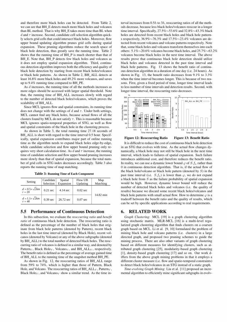
5.5 Performance of Continuous DetectionIn this subsection, we evaluate the reoccurring ratio and benefit

ratio of continuous black hole detection. The reoccurring ratio isdefined as the percentage of the number of black holes that orig-inate from black hole patterns (denoted by Pattern), recent blackholes in the last time interval (denoted by Black Hole), recent vol-canos (denoted by Volcano) or any of the above subgraphs (denotedby BH_ALL) to the total number of detected black holes. The reoc-curring ratio of volcanos is defined in a similar way, and denoted byPatternV , Black HoleV , VolcanoV , and BH_ALLV , respectively.The benefit ratio is defined as the percentage of average gained timeof BH_ALL to the running time of the snapshot method BH_PE.

As shown in Fig. 12, the reoccurring ratios of BH_ALL rangefrom 59% to 74%, which is higher than those of Pattern, BlackHole, and Volcano. The reoccurring ratios of BH_ALLV , PatternV ,Black HoleV , and VolcanoV show a similar trend. As the time in-

terval increases from 0.5h to 3h, reoccurring ratios of all the meth-ods decrease, because less black holes/volcanos reoccur in a longertime interval. Specifically, 27.5%∼53.6% and 32.8%∼43.3% blackholes are detected from recent black holes and black hole pattern-s respectively, 36.9%∼76.3% and 17.5%∼23.4% volcanos are de-tected from recent volcanos and volcano patterns respectively. Notethat, some black holes and volcanos transform themselves into eachothers: 5.1%∼20.6% volcanos become black holes, and 25.7%∼63.2%volcanos become black holes in the next time interval. The aboveresults prove that continuous black hole detection should utilizeblack holes and volcanos detected in the past time interval andblack hole patterns. Fig. 13 shows the benefit ratio of continu-ous detection algorithm in a duration of one day (i.e. 24 hours). Asshown in Fig. 13, the benefit ratio decreases from 9.1% to 3.3%when the time interval becomes longer. This is because of two rea-sons. First, given a fixed period of time, longer time interval leadsto less number of time intervals and detection results. Second, withlonger time interval, the reoccurring ratio decreases.

0

50

100

150

200

250

300

350

0.5 1 1.5 2 2.5 3

Reo

ccur

ring

Rat

io

Time Interval (hour)

%

BH_ALLBlack Hole

VolcanoPattern

BH_ALLVBlack HoleV

VolcanoVPatternV

Figure 12: Reoccurring Ratio

0

2

4

6

8

10

0.5 1 1.5 2 2.5 3

Ben

efit

Rat

io

Time Interval (hour)

%

BH_ALL vs. BH_PE

Figure 13: Benefit RatioIt is difficult to reduce the cost of continuous black hole detection

in an STG that evolves with time. As the actual flow changes dy-namically, a black hole may not still be black hole in the next timeinterval, which leads to failures of spatial expansion. Such failureintroduces additional cost, and therefore reduces the benefit ratio.In reality, we can use a dynamic lower bound ϕ of S.fa rather than0 in continuous detection algorithm. That is, if the actual flow ofthe black hole/volcano or black hole pattern (denoted by S) in thepast time interval (i.e. S.fa) is lower than ϕ, we do not expanda black hole from S as the failure probability of spatial expansionwould be high. However, dynamic lower bound will reduce thenumber of detected black holes and volcanos (i.e. the quality ofresults) because we discard some recent black holes/volcanos andblack hole patterns with small actual flow. How to determine ϕ is atradeoff between the benefit ratio and the quality of results, whichcan be set by specific applications according to real requirements.

6. RELATED WORKGraph Clustering: MCL [19] is a graph clustering algorithm

using stochastic matrix. MLR-MCL [16] is a multi-level regu-larized graph clustering algorithm that finds clusters on a coarsengraph based on MCL. Li et al. [9, 10] formulated the problem ofmining black hole and volcano patterns (i.e. clusters) in a largedirected graph, and proposed two pruning schemes to guide themining process. There are also other variants of graph clusteringbased on different measures for identifying clusters, such as at-tributed graph clustering [25], modularity-based graph clustering[1], density-based graph clustering [17] and so on. Our work d-iffers from the above graph mining problems in that it employs adifferent cluster measure (i.e. flow and spatio-temporal constraints)to detect black holes/volcanos in an STG instead of a static graph.

Time-evolving Graph Mining: Liu et al. [11] proposed an incre-mental algorithm to efficiently mine significant subgraphs in evolv-

ing graphs. A constraint-based pattern mining approach was pro-posed to find pseudo-cliques in dynamic graphs [15]. In [6], Lahiriet al. proposed an efficient pattern-tree-based algorithm to mineperiodically recurring interaction patterns in dynamic networks. Arecent work [14] deals with query processing over historical evolv-ing graph sequences to obtain interesting information from vari-ous query results. Differently, since spatio-temporal graph has spa-tial properties, our problem should consider spatio-temporal con-straints in black hole and volcano detection.

Grouping Traveling Behavior: The problem of density queryingfor moving objects finds out regions that have objects higher than athreshold in a given time interval [3]. Jensen et al. [4] generalizedthe problem to a dense region query with fixed shape. The differ-ences between density querying [3, 4] and our work are: 1) A denseregion is not necessary to be a black hole or volcano, and vice ver-sa. For example, a dense region is not a black hole if all the movingobjects finally move out of the regions within the time interval. 2)The irregular shape black holes/volcanos cannot be found by [3, 4]even if we change the definition of density from high concentrationof objects to high actual flow. Since [3, 4] consider fixed shape re-gion as a whole, these methods fail to detect black holes with irreg-ular shapes because a fixed shape region may include other edgeswith negative actual flows than edges within the irregular shape re-gion. Another branch of research is to discover a group of objectsthat move together for a certain time period (i.e. trajectory cluster-ing), such as convoy [5], swarm [8], traveling companion [18] andgathering [22]. However, black holes are not necessarily formed bya group of similar trajectories.

Spatio-Temporal Data Mining: Mathioudakis et al. [12] intro-duced scalable algorithms to identify spatial information bursts.Lappas et al. [7] presented a framework for simultaneously track-ing the spatial and temporal burstiness of terms. Note that, ourproblem is more challenging than the problem of identifying spatio-temporal bursts which ignore graph topology of spatial regions.

Recently, Pan et al. [13] studied the problem of detecting and de-scribing traffic anomalies using crowd sensing with human mobili-ty and social media data. Chen et al. [2] developed nonparametriclearning methods to learn dynamic graph structures from spatial-temporal data. There is plenty of literature on trajectory patternmining [23], aiming to analyze the mobility patterns of moving ob-jects. The problem definition of our work is different from priorworks which only consider the total amount of flow while ignorethe inflow and outflow of black holes/volcanos.

7. CONCLUSIONSIn this paper, we model human mobility data by an STG, from

which we detect urban black holes. Case study on Beijing taxicabdata demonstrates that our method can instantly find urban anoma-lies (e.g. football matches and concerts in Beijing Worker’s Stadi-um) that faciliate early warning of traffic congestions and tempo-rary traffic control, and human mobility patterns (e.g. the patternsaround Beijing South Railway Station) that help improve the ur-ban planning of Beijing. Case study on Bike trip data shows thatthe instantly detected black holes and volcanos can assist real-timescheduling of bikes, and the black hole/volcano patterns help opti-mize the deployment and site selection of bike stations. Moreover,our method outperforms baseline methods by reducing at least 68%running time and detecting 10 times more black holes. Comparedto the black hole detection in a time interval, our continuous detec-tion algorithm saves more than 9% total computational cost.

In the future, we would like to apply our method to Call DetailsRecords. The detected black holes would indicate the emergingevents, helping avoid potential risks of public safety.

AcknowledgmentsThe research is supported by NSFC under Grant 61303025, 61572488,863 project under grant 2015AA015402, NSFC (Key Program) un-der grant 61532010, Beijing Higher Education Young Elite TeacherProject (YETP0016), and the Fundamental Research Funds for theCentral Universities.

8. REFERENCES[1] U. Brandes, D. Delling, M. Gaertler, R. Gorke, M. Hoefer,

Z. Nikoloski, and D. Wagner. On modularity clustering. IEEE Trans.on Knowledge and Data Engineering, 20(2):172–188, 2008.

[2] X. Chen, Y. Liu, H. Liu, and J. G. Carbonell. Learning spatial-temporal varying graphs with applications to climate data analysis.In Proc. of AAAI, 2010.

[3] M. Hadjieleftheriou, G. Kollios, D. Gunopulos, and V. J. Tsotras.On-line discovery of dense areas in spatio-temporal databses. InProc.of SSTD, 2003.

[4] C. S. Jensen, D. Lin, B. C. Ooi, and R. Zhang. Effective densityqueries on continuously moving objects. In Proc. of ICDE, 2006.

[5] H. Jeung, M. L. Yiu, X. Zhou, C. S. Jensen, and H. T. Shen.Discovery of convoys in trajectory databases. PVLDB,1(1):1068–1080, 2008.

[6] M. Lahiri and T. Y. Berger-Wolf. Periodic subgraph mining indynamic networks. Knowledge and Information Systems, 24(3),2010.

[7] T. Lappas, M. R. Vieira, D. Gunopulos, and V. J. Tsotras. On thespatiotemporal burstiness of terms. PVLDB, 5(9):836–847, 2012.

[8] Z. Li, B. Ding, J. Han, and R. Kays. Swarm: Mining relaxedtemporal moving object clusters. PVLDB, 3(1-2):723–734, 2010.

[9] Z. Li, H. Xiong, and Y. Liu. Mining blackhole and volcano patternsin directed graphs: A general approach. Data Mining and KnowledgeDiscovery, 2012(25), 2012.

[10] Z. Li, H. Xiong, Y. Liu, and A. Zhou. Detecting blackhole andvolcano patterns in directed networks. In Proc. of ICDM, 2010.

[11] Z. Liu, J. X. Yu, Y. Ke, and X. Lin. Spotting significant changingsubgraphs in evolving graphs. In Proc. of ICDM, 2008.

[12] M. Mathioudakis, N. Bansal, and N. Koudas. Identifying, attributingand describing spatial bursts. PVLDB, 3(1-2):1091–1102, 2010.

[13] B. Pan, Y. Zheng, D. Wilkie, and C. Shahabi. Crowd sensing oftraffic anomalies based on human mobility and social media. InProc.of GIS, 2013.

[14] C. Ren, E. Lo, B. Kao, X. Zhu, and R. Cheng. On querying historicalevolving graph sequences. In PVLDB, 2011.

[15] C. Robardet. Constraint-based pattern mining in dynamic graphs. InProc. of ICDM, 2009.

[16] V. Satuluri and S. Parthasarathy. Scalable graph clustering usingstochastic flows: applications to community discovery. In Proc. ofKDD, pages 737–746. ACM, 2009.

[17] J. Šíma and S. E. Schaeffer. On the np-completeness of some graphcluster measures. In Proc. of SOFSEM, pages 530–537. Springer,2006.

[18] L.-A. Tang, Y. Zheng, J. Yuan, J. Han, A. Leung, C.-C. Hung, andW.-C. Peng. On discovery of traveling companions from streamingtrajectories. In Proc. of ICDE, 2012.

[19] S. Van Dongen. Graph clustering via a discrete uncoupling process.SIAM Journal on Matrix Analysis and Applications, 30(1):121–141,2008.

[20] X. Yan and J. Han. gspan: Graph-based substructure pattern mining.In Proc. of ICDM, 2002.

[21] J. Yuan, Y. Zheng, C. Zhang, X. Xie, and G. Sun. An interactive-voting based map matching algorithm. In Proc. of MDM, 2010.

[22] K. Zheng, Y. Zheng, N. J. Yuan, and S. Shang. On discovery ofgathering patterns from trajectories. In Proc. of ICDE, 2013.

[23] Y. Zheng. Trajectory data mining: An overview. ACM Trans. onIntelligent Systems and Technology, 2015.

[24] Y. Zheng, L. Capra, O. Wolfson, and H. Yang. Urban computing:concepts, methodologies, and applications. ACM Trans. onIntelligent Systems and Technology, 2014.

[25] Y. Zhou, H. Cheng, and J. X. Yu. Graph clustering based onstructural/attribute similarities. In Proc. of VLDB Conference, 2009.