Detecting external forces on an autonomous lawn …liu.diva-portal.org/smash/get/diva2:1095736/FULLTEXT01.pdf · 1 Introduction 1.1 Background Husqvarna Automower consist of a chassis

Master of Science Thesis in reglerteknikDepartment of Electrical Engineering, Linköping University, 2017

Detecting external forces onan autonomous lawnmowing robot with inertial,wheel speed and wheelmotor currentmeasurements

Gustav Norin

Master of Science Thesis in reglerteknik

Detecting external forces on an autonomous lawn mowing robot with inertial,wheel speed and wheel motor current measurements

Gustav Norin

LiTH-ISY-EX–17/5034–SE

Supervisor: Oskar Ljungqvistisy, Linköpings universitet

Mikaela ÅhlénHusqvarna AB

Examiner: Fredrik Gustafssonisy Linköpings universitet

Division of Automatic ControlDepartment of Electrical Engineering

Linköping UniversitySE-581 83 Linköping, Sweden

Copyright © 2017 Gustav Norin

Abstract

An autonomous lawn mowing robot moves around randomly within an area en-closed by a magnetic wire and makes decision based on sensor information. Toensure human and animal safety it is essential that the robotic lawn mower candetect and stop if, for instance, it is being lifted by a human. This thesis takes alook at how on-board sensors could be used to detect a few critical events, herecalled fault cases. Data such as acceleration, angular velocity and motor currentsare recorded and then used to develop three methods for detection briefly de-scribed below.

The Odometry method uses constraints on valid movement of the robotic lawnmower and a fault case is detected if estimated velocity in global coordinates vio-lates these constraints. The pitch angle relationship estimates the relation betweenelectrical currents needed to drive the robotic lawn mower at a certain speedin certain pitch angle. When the electrical currents corresponding to a certainpitch angle according to the relation deviates from measured currents a fault casewould be detected. The frequency method is based on the idea that disturbances onsignals caused by uneven ground should decrease when the robotic lawn moweris lifted or held. The method would then detect this damping of disturbances byexamining frequency content.

The best method is the pitch angle relationship while the other two proposedmethods have potential but would need higher sampling frequencies and addi-tional signals to fully perform satisfactorily. With additional information such asposition of the robotic lawn mower the estimation of the global velocities couldbe significantly improved which in turn would improve the odometry methodand serve as a complement to the current pitch angle relation. The frequencymethods would also be valid if the sampling frequencies were much higher, some-thing that might not be as cost efficient as needed to make the method profitable.

iii

Acknowledgments

The thesis suggestion was provided by Husqvarna AB and I would like to give spe-cial thanks to the following persons for helping me throughout the work.

• Jonas Rangsjö, Husqvarna AB

• Oskar Ljungqvist, supervisor, Linköping University

• Mikaela Åhlén, supervisor, Husqvarna AB

• Fredrik Gustafsson, Examiner, Linköping University

Linköping, August 2016Gustav Norin

v

Contents

Notation ix

1 Introduction 11.1 Background . . . . . . . . . . . . . . . . . . . . . . . . . . . . . . . 11.2 Purpose . . . . . . . . . . . . . . . . . . . . . . . . . . . . . . . . . . 11.3 Conditions and limitations . . . . . . . . . . . . . . . . . . . . . . . 21.4 Objectives . . . . . . . . . . . . . . . . . . . . . . . . . . . . . . . . 21.5 Method . . . . . . . . . . . . . . . . . . . . . . . . . . . . . . . . . . 21.6 Method limitation . . . . . . . . . . . . . . . . . . . . . . . . . . . . 21.7 Related work . . . . . . . . . . . . . . . . . . . . . . . . . . . . . . . 3

2 Conditions 52.1 Equipment and software . . . . . . . . . . . . . . . . . . . . . . . . 52.2 Coordinate systems . . . . . . . . . . . . . . . . . . . . . . . . . . . 62.3 Kinematic constraints . . . . . . . . . . . . . . . . . . . . . . . . . . 62.4 Signals . . . . . . . . . . . . . . . . . . . . . . . . . . . . . . . . . . 9

3 Definition of external forces 133.1 Standing still . . . . . . . . . . . . . . . . . . . . . . . . . . . . . . . 13

3.1.1 Lift front . . . . . . . . . . . . . . . . . . . . . . . . . . . . . 143.1.2 Lift back . . . . . . . . . . . . . . . . . . . . . . . . . . . . . 143.1.3 Lift whole . . . . . . . . . . . . . . . . . . . . . . . . . . . . 153.1.4 Lift side . . . . . . . . . . . . . . . . . . . . . . . . . . . . . 153.1.5 Collision . . . . . . . . . . . . . . . . . . . . . . . . . . . . . 163.1.6 Wheel slip . . . . . . . . . . . . . . . . . . . . . . . . . . . . 16

3.2 Driving . . . . . . . . . . . . . . . . . . . . . . . . . . . . . . . . . . 163.2.1 Lift front . . . . . . . . . . . . . . . . . . . . . . . . . . . . . 163.2.2 Lift back . . . . . . . . . . . . . . . . . . . . . . . . . . . . . 173.2.3 Lift whole . . . . . . . . . . . . . . . . . . . . . . . . . . . . 183.2.4 Lift side . . . . . . . . . . . . . . . . . . . . . . . . . . . . . 183.2.5 Collision . . . . . . . . . . . . . . . . . . . . . . . . . . . . . 193.2.6 Wheel slip . . . . . . . . . . . . . . . . . . . . . . . . . . . . 19

3.3 Fault case summary . . . . . . . . . . . . . . . . . . . . . . . . . . . 20

vii

viii Contents

4 Detection methods 234.1 Odometry . . . . . . . . . . . . . . . . . . . . . . . . . . . . . . . . . 24

4.1.1 Integrate accelerometer data . . . . . . . . . . . . . . . . . . 254.2 Pitch current relationship . . . . . . . . . . . . . . . . . . . . . . . 26

4.2.1 Pitch and current in static relationship . . . . . . . . . . . . 264.2.2 Pitch and current dynamic relationship . . . . . . . . . . . 30

4.3 Frequencies . . . . . . . . . . . . . . . . . . . . . . . . . . . . . . . . 32

5 Evaluation & results 335.1 Method evaluation . . . . . . . . . . . . . . . . . . . . . . . . . . . . 33

5.1.1 Odometry . . . . . . . . . . . . . . . . . . . . . . . . . . . . 335.1.2 Pitch current relationship . . . . . . . . . . . . . . . . . . . 365.1.3 Frequencies . . . . . . . . . . . . . . . . . . . . . . . . . . . 40

5.2 Standing still . . . . . . . . . . . . . . . . . . . . . . . . . . . . . . . 435.3 Driving . . . . . . . . . . . . . . . . . . . . . . . . . . . . . . . . . . 45

6 Conclusions 476.1 Summary . . . . . . . . . . . . . . . . . . . . . . . . . . . . . . . . . 476.2 Future work . . . . . . . . . . . . . . . . . . . . . . . . . . . . . . . 48

Bibliography 49

ix

x Notation

Notation

Notations that will be used in the report

Notation Description

Ts Sampling intervalθ pitch-angleφ roll-angleψ yaw-angleθ pitch angular velocity or pitch-rateφ roll angular velocity or roll-rateψ yaw angular velocity or yaw-rate

X, Y , Z Global coordinate systemx, y, z Local coordinate systemv Linear velocity of the robotic lawn mower (along x,

same as Vx)Va Velocity along coordinate-axis a ∈ {X, Y , Z, x, y, z}Aa Acceleration along coordinate-axis a ∈ {X, Y , Z, x, y, z}ωj Angular speed of wheel j, j = 1, 2ij Current on motor j = 1, 2

d = 0.04645 Distance between wheels in metersr = 0.1225 Wheel radius in meters

()k Variables or parameters with subscript k denote dis-crete time

()(t) Variables or parameters followed by (t) denote contin-uous time

g = 9.82 Gravitational acceleration in m/s2

x The estimated stateP State covarianceJ Motor inertia in kgm2

K Torque in NmT Lj Load torque in Nm on motor j = 1, 2B Friction/damping-constantSP position of imuT O Turn origo, i.e the center of a coordinated turn

1Introduction

1.1 Background

Husqvarna Automower consist of a chassis and a cover. The wheels and theblades are attached to the chassis which also carries all electronics such as sen-sors and motors. The cover is on top of the chassis. The cover is connected tothe chassis by magnets which in turn that are equipped with hall effect sensors.If the cover is under an external force the connecting magnets will come loose,an event registered by the hall effect sensor. This is how external forces are de-tected by Husqvarna Automower today. If the cover could be removed this wouldreduce production materials and assembling steps ultimately leading to a lowerproduction costs for the company. This master thesis examines alternative waysof detecting external forces to remove the need of a cover. The thesis is performedat Linköping University in collaboration with Husqvarna AB.

1.2 Purpose

The purpose of this thesis is to explore and analyze alternative approaches for de-tecting external forces acting on an robotic lawn mower other than the approachdescribed in Section 1.1.

1

2 1 Introduction

1.3 Conditions and limitations

There is a specific setup of sensors and means of recording on the robotic lawnmower that is used in this thesis. To limit the scope of the work this setup will notbe altered with. Methods to be explored and analyzed are thus restricted in thesense that these will be developed from the specific setup and not from a generalperspective. Sensors and signals in the current setup are presented and describedin Chapter 2. Further the thesis is limited to cases when the robotic lawn moweris driving straight or standing still.

1.4 Objectives

The objectives of the thesis are:

• Develop methods or models that could detect the external forces defined inChapter 3 with the signals presented in Chapter 2.

• Document the limitations of developed methods.

• Examine and discuss how current setup might limit the detection possibili-ties.

1.5 Method

The thesis starts by searching for related previous work that could either inspireor reject ideas on how to solve the problem at hand. Data is then recordedwhile external forces are both present and not present and while the robotic lawnmower is both standing still and driving straight. The signals are compared togain knowledge of signal characteristics which can then be used to develop mod-els that accurately relate signals under valid movements but output contradic-tions while external forces are present, this is called fault diagnosis. Only oneof the external forces in Chapter 3 will be present at one time. The recordingsare performed in Robot Operating System (ros) with help from employees atHusqvarna AB while analyzes of data and model implementations are conductedin Matlab. Lastly limitations of developed models are discussed. All models as-sume an online implementation since external forces are supposed to be detectedas soon as they occur.

1.6 Method limitation

There are infinite many ways on how to apply external forces and hence there isa variety on how these forces effect available signals. However the variety is as-

1.7 Related work 3

sumed to have scaling affects meaning that the overall characteristics of a force’sinfluence do not change but the magnitude of said characteristics will vary. Infault diagnosis the magnitudes of various events are nonetheless of importanceand as a consequence this could become limitations for some models. The sub-ject itself is within a broad field of signal processing, modeling, estimation anddiagnosis, i.e. the subject is not a deeper evaluation or development of existingmethods or within a narrow technical field. Thus ideas, developed models andrelevant theories are inevitably based on the authors previous knowledge whichwould mean that there might be other more suitable solutions.

Another limitation is time which in this case is approximately 20 weeks.

1.7 Related work

Ivanic [6] was the closest match to this work even though the degree might beto low for using as a reference. [6] focuses on using the accelerometer to de-tect external forces where the main strategy was to compute a moving averageof accelerometer readings to detect collision. However the method seemed to beworking if the surface was flat and even and not otherwise. Most robotic lawnmowers can track its rotation and thereby detect when the rotation exceeds pre-set limits to avoid driving in steep terrain that could result in the robotic lawnmower falling over. Ståhl [6] suggests that the robotic lawn mower’s rotationallimit could used as a detection algorithm for when the robotic lawn mower waslifted. However all cases where a lift does not result in a rotation exceeding thelimit would not be detectable. [12] is a master thesis that look into collision de-tection of a robotic lawn mower at Husqvarna which suggests moving averageof electrical currents applied by the motors driving each wheel to detect colli-sion. The main difficulty seemed to be to account for slopes which could leadto harsh collisions before detection. In Sabatini and Genovese [11] the authorsdiscuss how to track vertical motion but compared to this thesis there is an ad-ditional measurement of pressure from a barometric altimeter, something that isnot available in this case. Other work that could relate to the topic of this thesis ismainly with the purpose to control the robotic lawn mower in a two-dimensionalenvironment and thus not directly related to detecting external forces.

2Conditions

This section will describe the general characteristics of the robotic lawn mower.These characteristics are: coordinate systems, relevant equipment, kinematic con-straints and measurable quantities (i.e. available signals).

2.1 Equipment and software

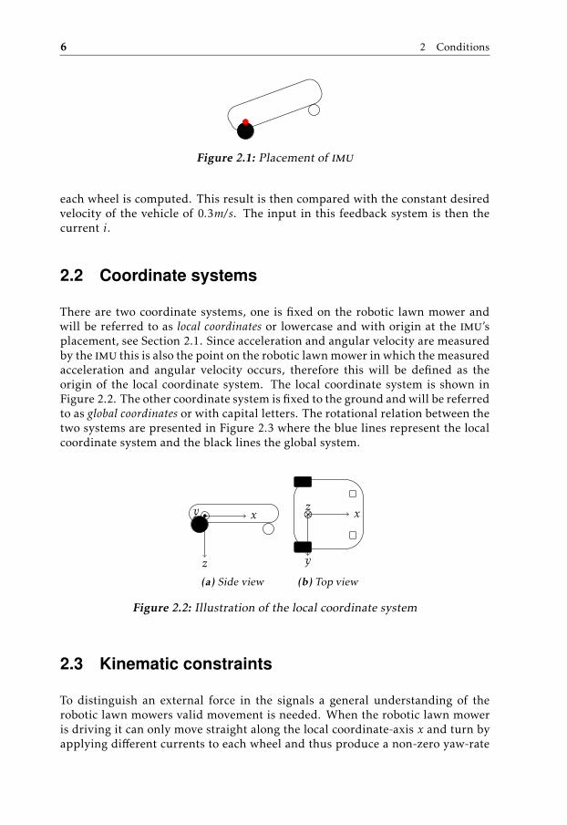
The robotic lawn mower is equipped with four wheels where the two at the backare fixed on the robotic lawn mower and are connected to two separate electricalmotors. The back wheel are illustrated as filled black circles or squares whendrawn in figures, see Figure 2.1. The two front wheels are orientable wheels orso called Caster-wheels and are illustrated as circles or squares when drawn infigures, see Figure 2.1.

As mentioned in Section 1.1 there is a cover on top of the robotic lawn mowerconnected with magnets to its chassis. When the cover moves in relation to thebody the magnets come loose and thus an external force is detected.

There is an Inertial Measurement Unit (imu) placed in the middle between thetwo back-wheels as illustrated in Figure 2.1. What is included in the imu is listedin Table 2.4.

Besides the physical aspects described above there is also software of interest.The computer programs running on the robotic lawn mower are written in C++and implemented with ros.

There is also a Proportional, Integral & Differential regulator (pid) implemented.The angular velocity of the wheels are measured from which the linear velocity of

5

6 2 Conditions

Figure 2.1: Placement of imu

each wheel is computed. This result is then compared with the constant desiredvelocity of the vehicle of 0.3m/s. The input in this feedback system is then thecurrent i.

2.2 Coordinate systems

There are two coordinate systems, one is fixed on the robotic lawn mower andwill be referred to as local coordinates or lowercase and with origin at the imu’splacement, see Section 2.1. Since acceleration and angular velocity are measuredby the imu this is also the point on the robotic lawn mower in which the measuredacceleration and angular velocity occurs, therefore this will be defined as theorigin of the local coordinate system. The local coordinate system is shown inFigure 2.2. The other coordinate system is fixed to the ground and will be referredto as global coordinates or with capital letters. The rotational relation between thetwo systems are presented in Figure 2.3 where the blue lines represent the localcoordinate system and the black lines the global system.

x

z

y

(a) Side view

x

y

⊗z

(b) Top view

Figure 2.2: Illustration of the local coordinate system

2.3 Kinematic constraints

To distinguish an external force in the signals a general understanding of therobotic lawn mowers valid movement is needed. When the robotic lawn moweris driving it can only move straight along the local coordinate-axis x and turn byapplying different currents to each wheel and thus produce a non-zero yaw-rate

2.3 Kinematic constraints 7

X

Y

Z

xy

z

ψ, yaw

(a) Rotation around z results in a yaw-anglealso denoted ψ

Z

X

Y

zx

y

θ, pitch

(b) Rotation around y results in a pitch-anglealso denoted θ

Y

Z

X

xy

z

φ, roll

(c) Rotation around x results in a roll-anglealso denoted φ

Figure 2.3: Rotaion of the local coordinate system relative the global coordi-nate system

ψ. Hence the robotic lawn mower is restricted on the angular velocities φ and θas well as on the linear velocities along y and z. Consequently the robotic lawnmower should have two degrees of freedom and four nonholomonic constraints[5], [1].

To compute the constraints the kinematics of the robotic lawn mower must besorted out. To simplify the kinematics computation we will first look at the two-dimensional case as seen in Figure 2.4. As previously stated the robotic lawnmower can control its rotation ψ and its translation along x.

The reader is referred to Figure 2.4 for notations used in the following calcula-tions. For calculation of the yaw rate ψ lets assume that the robotic lawn mowertraveled from time t0 until time t1 and during the travel turned ψ radians aroundT O, which also is the yaw-angle ψ, and thus traveled along the arc s, see Figure

8 2 Conditions

2.4. The calculation of ψ thus become

dsdt

=dψ

dtR⇔ (2.1a)

v = ψR⇔ (2.1b)vR

= ψ (2.1c)

and the calculation of v becomes

v =v1 + v2

2

/v1 = w1

2π2rπ = w1rv2 = w2

2π2rπ = w2r

/= (2.2a)

=r(w1 + w2)

2(2.2b)

Using (2.2) in (2.1c) yields

ψ =w1r + w2r

21R

(2.3)

Finally R needs to be expressed in known quantities, thus the ratio between v1and v2 is computed.

v1

v2

(2.1b)=

ψR1

ψR2

Figure 2.4=

R + d2

R − d2

⇔ v1(R − d2

) = v2(R +d2

)⇔ (2.4a)

R(v1 − v2) =d2

(v1 + v2)⇔ (2.4b)

1R

=2dv1 − v2

v1 + v2=

2d

r(w1 − w2)r(w1 + w2)

=2dw1 − w2

w1 + w2(2.4c)

Inserting (2.4c) in (2.3) yields

ψ =r(w1 + w2)

22dw1 − w2

w1 + w2=r(w1 − w2)

d(2.5)

In [3] the gravitational force which only has a magnitude in global coordinate Zcan be rotated to the local coordinate system by multiplying the rotational matrixQ in (2.6) with the Z-component.

Q =

cos θ cosψ cos θ sinψ − sin θsinφ sin θ cosψ − cosφ sinψ sinφ sin θ sinψ + cosφ cosψ sinφ cos θcosφ sin θ cosψ + sinφ sinψ cosφ sin θ sinψ − sinφ cosψ cosφ cos θ

(2.6)

Instead of rotating from global coordinates to local coordinates one can rotate theother way around by instead multiply Q−1 with a component of the local systemto get it in global coordinates. [3] further states that Q−1 = QT . and the velocityin the local coordinate system is thus multiplied by QT . Since the velocity in thelocal coordinate system is strictly constrained to x the second and third column

2.4 Signals 9

of the rotational matrix will be multiplied by 0 and thus the kinematics of therobotic lawn mower can be written as in (2.7).VXVY

VZ

=

cos θ cos(ψ)cos θ sin(ψ)− sin θ

r(w1 + w2)2

(2.7a)

ψ =r(w1 − w2)

d(2.7b)

Multiplying (2.6) with a vector of global velocities [VX , VY , VZ ]T yields

Vx = cos θ cosψVX + cos θ sinψVY − sin θVZVy = (sinφ sin θ cosψ − cosφ sinψ)VX + (sinφ sin θ sinψ+

cosφ cosψ)VY + sinφ cos θVZVz = (cosφ sin θ cosψ + sinφ sinψ)VX + (cosφ sin θ sinψ−

sinφ cosψ)VY + cosφ cos θVZ

(2.8)

However Vy and Vz should be 0 and thus the two constraints have been computed,these are seen in (2.9).

(sinφ sin θ cosψ − cosφ sinψ)VX + (sinφ sin θ sinψ+cosφ cosψ)VY + sinφ cos θVZ = 0

(cosφ sin θ cosψ + sinφ sinψ)VX + (cosφ sin θ sinψ−sinφ cosψ)VY + cosφ cos θVZ = 0

(2.9)

The solution to (2.9) is further given in (2.7a).

2.4 Signals

The measurable quantities or signals that can be used to perform fault diagnosison the system is listed in Table 2.1 below

10 2 Conditions

Table 2.1: Available measured signals on the auto mower.

Sensor Description

Accelerometer Placed inside the imu and measures ac-celeration in x, y and z with a samplingfrequency fs of 180Hz.

Gyroscope Placed inside the imu and measures an-gular velocities ψ, φ and θ with a sam-pling frequency fs of 180Hz.

Quaternions The imu sensor have a quaternions esti-mation implemented by the manufactur-ers and is also delivered with a samplingfrequency fs of 180Hz.

Motor currents The motor current can be measured witha sampling frequency fs of 18Hz.

Wheel angular velocities The angular velocities by the two back-wheels are measured with a respectiveHall effect sensor, each with a samplingfrequency fs of 18Hz.

2.4 Signals 11

t0

s1

s

s2

w1 v1

w2 v2

SP

v

t1

w1

v1

w2

v2

SP

v

T O

d

R

R1

R2

ψ

ψ

Figure 2.4: Pitch current relationship figure

3Definition of external forces

This chapter will describe and specify the external forces that are of interest todetect.

Since we are not near any singularities, Euler angles will be used. Moreover theyrepresent the same thing and one need to simply use the definition, see [3] totranslate an angle to quaternions or vice versa. Quaternions or Euler angles areneeded for calculations of the kinematics and rotations but there would be nodifference whether the orientation is due to an external force or ground shapeand thus the these signals could not directly be used to detect an external force.The same goes for the angular velocities of the back-wheels though as a result ofthe feedback controller that keeps certain velocities on each wheel.

When discussing movement of the robotic lawn mower it is actually the move-ment of the imu that is discussed.

There should also be noted that each case is simplified to a movement in only oneaxis or a rotation around only one axis.

3.1 Standing still

When no control command has been sent telling the robotic lawn mower to drivethere should be no movement at all. Meaning that all available signals should beconstant.

13

14 3 Definition of external forces

3.1.1 Lift front

The lift is illustrated in Figure 3.1. When lifted at front there would be a non-

X

Z

(a) Global co-ordinate sys-tem

x

z

y

(b) Not lifted

x

z

y

(c) Lifted at front

Figure 3.1: Illustration of a front lift and a similar though valid case whenthe robotic lawn mower is standing still.

zero angular velocity and the gravitational acceleration would decrease in z andincrease in y, thus in conclusion the lift should be possible to detect simply bysetting a threshold indicating that one of the signals has changed.

3.1.2 Lift back

Lifting back while standing still would be similar as when lifted at front, therewould be a non-zero angular velocity and the gravitational acceleration would de-crease in z and increase in y, thus in conclusion the lift should be possible to de-tect simply by setting a threshold indicating that one of the signals has changed.The lift is illustrated in Figure 3.2.

X

Z


x

z

y

(b) Not lifted

x

z

y

(c) Lifted at back

Figure 3.2: Illustration of a back lift and a similar though valid case whenthe robotic lawn mower is standing still.

3.1 Standing still 15

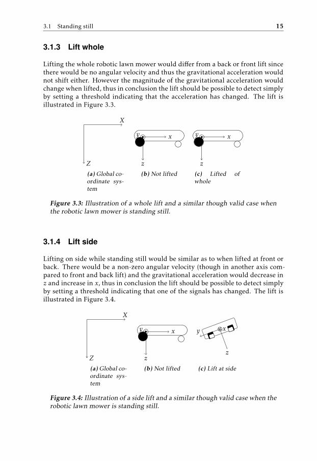
3.1.3 Lift whole

Lifting the whole robotic lawn mower would differ from a back or front lift sincethere would be no angular velocity and thus the gravitational acceleration wouldnot shift either. However the magnitude of the gravitational acceleration wouldchange when lifted, thus in conclusion the lift should be possible to detect simplyby setting a threshold indicating that the acceleration has changed. The lift isillustrated in Figure 3.3.

X

Z


x

z

y

(b) Not lifted

x

z

y

(c) Lifted ofwhole

Figure 3.3: Illustration of a whole lift and a similar though valid case whenthe robotic lawn mower is standing still.

3.1.4 Lift side

Lifting on side while standing still would be similar as to when lifted at front orback. There would be a non-zero angular velocity (though in another axis com-pared to front and back lift) and the gravitational acceleration would decrease inz and increase in x, thus in conclusion the lift should be possible to detect simplyby setting a threshold indicating that one of the signals has changed. The lift isillustrated in Figure 3.4.

X

Z


x

z

y

(b) Not lifted

y

z

⊗x

(c) Lift at side

Figure 3.4: Illustration of a side lift and a similar though valid case when therobotic lawn mower is standing still.


3.1.5 Collision

A collision while standing still would be that something has hit the automover, de-pending on the impact acceleration and gyroscope data would be affected. Thusin conclusion the collision should be possible to detect simply by setting a thresh-old indicating that one of the signals has changed.

3.1.6 Wheel slip

A wheel slip while standing still would mean that the robotic lawn mower hasstarted to slide in some direction. The lift should be possible to detect simply bysetting a threshold indicating that one of the signals has changed.

3.2 Driving

In contrast to when the robotic lawn mower is standing still the signals will bechanging while driving.

3.2.1 Lift front

The lift is illustrated in Figure 3.5.

When the robotic lawn mower start to climb a hill the local coordinate system isshifted with the pitch angle and as a result of the kinematics in (2.7) the localvelocity in x would then have components in both Z and X, i.e the robotic lawnmower should move along Z and X. When the robotic lawn mower is lifted infront however there will be no movement along Z and thus there is a contrastwhich might be detectable if a velocity is produced with (2.7) and compared withhow the movement looks according to the accelerometer.

Concerning the motor currents there should be a higher demand when the roboticlawn mower climbs a hill to obtain constant speed. Therefore is seems likely thatthere is a relation between the motor currents and the angle θ. If a sufficientrelation between the currents and θ would be determined deviation could be de-tected and assumed to be caused by an external force. However the relation couldalso be subjected to ground surface, e.g. a hard dry surface without grass woulddemand less current than soft wet moss. Another impeding aspect could be thatthe lift hinders the robotic lawn mower to move forward and thus results in ahigher demand of current similar to a valid case.

3.2 Driving 17

A VXBB

C

D

E F

(a) Driving up over bump

VZ

VXVx

θ

(b) Driving when lifted at front

Figure 3.5: Illustration of a front lift and a similar though valid case whenthe robotic lawn mower is driving forward.

3.2.2 Lift back

The lift is illustrated in Figure 3.6.

Similar to the case 3.2.1 a climb down a hill would with the kinematics in (2.7)result in the local velocity to have components in both Z and X, i.e the roboticlawn mower should move along Z and X. When the robotic lawn mower is liftedat back however there will a positive velocity along Z, which should be negativesince the nose of the robotic lawn mower is pointing down. Additionally since thetwo back wheels are lifted of the ground the robotic lawn mower will stop eventhough the wheels are still turning. Thus there are two contrast which mightbe detectable if a velocity is produced with (2.7) and compared with how themovement looks according to the accelerometer.

Concerning the motor currents there should be a lower demand when the roboticlawn mower drives down a hill to obtain constant speed. Again indicating arelation between the motor currents and the angle θ. If a sufficient relation be-tween the currents and θ would be determined deviation could be detected andassumed to be caused by an external force. However for this case when bothwheels are off the ground and the demanded current would go down similar towhen when the robotic lawn mower is driving down a hill which could meanthat the contrast between the valid case and the lift is not sufficiently signifi-cant.


F ED

C

B Av

(a) Driving up over bump

VZ

VXVx

θ

(b) Driving when lifted at front

Figure 3.6: Illustration of a front lift and a similar though valid case whenthe robotic lawn mower is driving forward.

3.2.3 Lift whole

When lifting the whole robotic lawn mower straight in Z all angles and angularvelocities would remain the same. The accelerometer would show a peak in zcorresponding to the lift and the wheel current would drop. The contrasts herewould be that the according to the kinematics the robotic lawn mower is stilldriving straight forward but the accelerometer readings would indicate a stopsimilar to 3.2.2. The relation between motor current and pitch angle would saythat the current should remain the same since there is no pitch angle but thewheel currents still drop since they do not have traction to the ground.

3.2.4 Lift side

Lifting at a side would mean that one wheel loses traction to the ground and thecorresponding motor’s current would drop and the other motor’s current wouldincrease. A side lift would also mean that the rotation is around the oppositewheel compared to the side the lift occurs. Therefore this should show as a move-ment in y which would not be permitted under normal conditions.

3.2 Driving 19

3.2.5 Collision

There should be an acceleration in the opposite direction of the force, if it is afront collision stopping the automover there should be a negative acceleration inx. The wheel current would go up since the feedback controller is trying to makeup the external force hindering the robotic lawn mower.

3.2.6 Wheel slip

Similar as for the case of collision there should be an acceleration in the oppositedirection of the current heading. The electrical current would go down since thegrip has come lose and it does not take as much current to drive the wheels at acertain velocity.


3.3 Fault case summary

The fault cases are summarized with respective characteristics in table 3.1. Pro-posed methods are also included to indicate what methods could detect whatfault case. For further explanation of the methods the reader is referred to Chap-ter 4.

3.3 Fault case summary 21

Table 3.1

Driv-ing

Force Characteristic(s) Detection method

Odometry Load Frequency Changeinsignals

No Liftfront

Angle changeX X

Liftback

Angle changeX X

Liftwhole

Angle changeX X

Liftside

Angle changeX X

Colli-sion

Acceleration changeX

Wheelslip

Acceleration changeX

Yes Liftfront

Pitch angle non-zerobut no VZ . Pitch changenot corresponing tochange in demand ofelectrical current

X X

Liftback

Pitch angle non-zerobut no VZ . Stop in VX .Pitch change notcorresponing to changein demand of electricalcurrent

X X X

Liftwhole

Stop in VX . Change indemand of electricalcurrent but no changein pitch.

X X X

Liftside

Demand of electricalcurrent different ofeach wheel.

X X X

Colli-sion


X X

Wheelslip


X X

4Detection methods

Given the definition of the external forces and their signal characteristics in Chap-ter 3 and the constraints and knowledge of the robotic lawn mowers propermovement this chapter investigate three ideas an external force might be de-tected.

All methods would ultimately create residuals based on probabilistic diagnosissince there are measurement noise present, see [2]. The distribution of these willbe assumed Gaussian, with expected value (µ) and variance (σ ) determined bytheir definitions taken from [7] and seen in (4.1b) and (4.1c) respectively. The ex-pected value and variance will be calculated from data not influenced by externalforces.

ri ∼ N (µi , σi) (4.1a)

µi = E(ri) =1N

N∑n=1

ri,n i = 1, 2 (4.1b)

σi = E((ri − µi)2) = E(r2i ) − 2µi + µ2

i =1N

N∑n=1

r2i,n − 2µi + µ2

i i = 1, 2 (4.1c)

The residuals created should have the expected value of zero and thus a Hypoth-esis test can be constructed according to (4.2). Moreover the variance, σ , will beassumed the same whether an external force is acting on the robotic lawn moweror not meaning that the expected values is what is going to be altered by an exter-nal force.

H0 :r ∼ N (0, σ ) No external force (4.2a)

H1 :r ∼ N (µ , 0, σ ) External force (4.2b)

23

24 4 Detection methods

The next step is to select a threshold so that the probability of both false andmissed detection is low. This is a trade off since a lower threshold would resultin more detections and thereby more false alarms whereas a higher thresholdwould give less detection and thus more missed detections. For the robotic lawnmower it is crucial to detect actual lifts meaning that false alarm is preferred overmissed detection. Let α denote the probability of false detection and T denotethe threshold, the relation between these two is then according to (4.3). Theequation states that the probability of the residual being larger than the thresholdprovided that no actual external force is present, i.e. a false detection, equals adesired value of α. Since false detection is preferred over missed detection arelative high alpha is to be selected. [2]

α = P (|r | > T |µ = 0)⇔ (4.3a)

α = P (r < −T |µ = 0) + P (r > T |µ = 0)⇔ (4.3b)

α = 2P (r > T |µ = 0)⇔ (4.3c)

α = 2(1 − P (r < T |µ = 0))⇔ (4.3d)

1 − α2

= P (r < T |µ = 0) (4.3e)

(4.3) is then standardized to µ = 0 and σ = 1 by subtracting µ and dividing bythe standard deviation,

√σ , from both sides of the inequality. The result is seen

in (4.4).

1 − α2

= P

(r√σ<T√σ|µ = 0

)(4.4)

When α is selected the threshold T can be computed by using a normal distri-bution table which relates probabilities with thresholds for a stochastic variablewith standard normal distribution.

4.1 Odometry

One idea would be to estimate the velocity of the imu along the global verticalaxis X, Y and Z and then insert the estimated signals in the constraints given in(2.9).

With current signals there are two ways to compute or estimate VX ,VY and VZ .The accelerometer values could be rotated to global coordinates and then inte-grated, however the constraint in (2.9) are in fact a rotation of global to localcoordinates and thus the constraint could be checked directly by integrating theaccelerometer data to get the local velocities, where Vy and Vz should be zero.The second way would be to compute the velocities with the kinematics equation,(2.7), but once again the constraints are simply rotating these back to local ve-locities meaning that this would result in a rotation to global velocities and thenback to local, a procedure where no deviations would be seen. It seems plausibleto use a filter to estimate the global velocities such as a Kalman filter since there

4.1 Odometry 25

are two independent ways to compute global velocities. However the kinematicsequation will not provide valid results if there is an external force present. More-over it is the contrast between ways to obtain global velocities that can be usedto detect external forces and in a Kalman filter the information of both wouldbe used resulting in a vanished contrast between valid and invalid movement.Therefore no Kalman filter will be used.

Before the accelerometer data can be used the gravitational influence needs tobe removed. The gravitational components in the local coordinate system can becalculated by multiplying g with Q in (2.6) and thus produce the local accelera-tions xy

z

=

xyz

− Q ∗00g

(4.5)

There is also biases on the signals which should be taken into account. The biasof the signal will be considered as the mean of the data of each signal collectedfrom when the robotic lawn mower is standing still.

Since the data is sampled a discretization of the integration is needed. Usingzero-order-hold as in [9] the integration becomes as shown in (4.6).

Vk = Vk−1 + Ak ∗ Ts (4.6)

4.1.1 Integrate accelerometer data

As previously claimed the velocities VX ,VY and VZ could be calculated by firstrotate the accelerometer data (Ax,Ay and Az) with QT to obtain AX ,AY and AZwhich would then be integrated to get the global velocities. On the other handthe constraint is simply a rotation back to local coordinates and the test wouldonly need to integrate accelerometer data to see if there is velocities in y or z arenot zero.


4.2 Pitch current relationship

Another idea is to try and find the relation between motor currents and the pitchangle θ. It should be noted that a feedback controller is implemented to keep therobotic lawn mower at desired local velocity which will complicate or perhapsimpede a sufficient estimation.

4.2.1 Pitch and current in static relationship

The idea with this model is that when the wheels are not affected by an externalforce the only thing that would demand more or less current to keep the samespeed is the pitch angle, provided that no turning is performed. Another thingthat could influence needed current is the ground surface. For instance wet mosswould require higher currents than dry wood to keep the same speed. Howeverthe influence of a turn is neglected and the data is naturally collected when noturn is performed. Therefore a simple relation between the motor currents andthe pitch angle based on force equilibrium seen in [10] is presented below. More-over the model is only assumed to be true if the robotic lawn mower is movingforward.

Kik = mg sin(θk) + F0 + ekk = 1, . . . , Nek ∼ N (0, σe,k)

(4.7)

K is a constant that multiplied by ik result in the force driving the robotic lawnmower forward. The first term on the right hand side of (4.7) is the influence ofthe gravitation, F0 is the fundamental inertia of the wheels and ek is assumed tobe white Gaussian noise.

If θk is assumed fixed the model becomes linear and (4.7) can be rewritten as.

ik = aAk + F + ek (4.8)

where

a =1K

(4.9a)

Ak = mg sin(θk) (4.9b)

F =F0

K(4.9c)

Measurement of ik and Ak for k = 1, ..., N yieldsi1...iN

=

A1 1...AN 1

(aF

)+

e1...eN

(4.10)

4.2 Pitch current relationship 27

and then using vector and matrix notations

Y =

i1...iN

(4.11a)

H =

A1 1...AN 1

(4.11b)

Θj =(aF

)(4.11c)

ej =

e1...eN

(4.11d)

the model given in (4.8) can be written as

Y = HΘ + e (4.12)

where the noise e is uncorrelated and the noise vector e thus have the standarddeviation R shown in (4.13).

R =

σe,1

. . .σe,N

(4.13)

To estimate Θ the Least Square (LS) method will be used as defined in [3]. Thecost function V is defined as

V (Θ) = (Y −HΘ)T (Y −HΘ) (4.14)

and the estimation of Θ becomes

Θ = arg minΘ

V (Θ) (4.15)

Solving V (Θ) for Θ as shown below.

V (Θ) = (Y −HΘ)T (Y −HΘ) = (4.16a)

YTY − YTHΘ − ΘTHTY + ΘTHTHΘ = (4.16b)

YTY − 2ΘTHTY + ΘTHTHΘ (4.16c)

(4.16c) is then derived with respect to Θ and set equal to 0 to find the minimum


of V (Θ), these calculations are performed below.

dVdΘ

= −2HTY + 2HTHΘ = 0⇔ (4.17a)

HTHΘ = HTY⇔ (4.17b)

Θ = (HTH)−1HTY (4.17c)

The second derivative of (4.16c) is

d2V

dΘ2 = 2HTH > 0 (4.18)

which is always larger than zero since it is a square product and thus (4.14)will have a minimum for the estimated Θ. If the data have been generated bythe model for true parameter values Θo then the estimation in (4.17c) becomes

Θ = (HTH)−1HTY = (4.19a)

= (HTH)−1HT (HΘo + e) = (4.19b)

= Θo + (HTH)−1HT e (4.19c)

and thus

E(Θj ) = Θoj (4.20a)

Cov(Θj ) = (HTH)−1(HTRH)(HTH)−1 (4.20b)

Three sets of data are concatenated and will be used to estimate Θ. To smoothout the disturbances on each current and make the estimation less influencedby outliers the two currents sent to the left and right wheel respectively will beadded up and then divided by two to get the mean current for each time instance.This approach should be valid since the thesis is restricted to driving straightand thus the model parameters in (4.7) should be the same for each motor. Theconcatenated data of current and gravitational influence (Ak in (4.9b)) is seen inFigure 4.1a respectively 4.1b.

From the estimated Θ a current is simulated with data from another set otherthan the data used for estimation and a residual is calculated as defined in (4.21).The result is seen in Figure 4.2.

A residual can then be computed as

r = Y −HΘ (4.21)


(a) Mean current of left and right motor used in estimation of Θ in(4.19a) (Y)

(b) Gravitational effect used in estimation of Θ in (4.19a)

Figure 4.1: Data used for estimation of Θ


Figure 4.2: Validation of the estimation of Θ

4.2.2 Pitch and current dynamic relationship

There is a feedback controller setting the current to keep desired speed whichwould mean that the current is depending on previous values and thus the staticmodel in (4.7) might not be sufficient. To see if there is a dynamic relation be-tween the current and pitch an Auto-Regressive with an eXtra input (ARX) -model,see [4], will be modeled.

The general ARX-model using the same force equilibrium that was used whensetting up (4.7) is presented in (4.22)

ik + · · ·+ anik−n = b1(mg sin(θk)− c) + · · ·+ bm(mg sin(θk−m)− c) + F0 + e(t) (4.22)

where e(t) is white noise, c is a time delay and n and m are not yet decided modelorders. The delay c is here placed outside sin because mgsin(θ) will be seen as afixed value to keep the model linear. Using the notations

ϕk = (ik−1 . . . ik−n mg sin(θk) − c . . . mg sin(θk−m) − c 1)T (4.23a)

Θ = (a1 . . . an b1 . . . bm F0) (4.23b)

a prediction ik of ik can be formulated as

ik = ϕTk Θ (4.24)

end thus the prediction error is defined as

ik − ϕTk Θ (4.25)


The estimated model would have two inputs, mg sin(θ) and F0, which will bereferred to as u1 and u2 respectively. The estimation is performed by varyingthe model orders n, m and the delay for u1 where the combination that resultsin the lowest prediction error are selected. In a general sense there could alsobe a model order above one and a delay on u2, however this is a constants, notdepending on previous values, representing a fundamental ampère need to drivethus have an immediate effect on the current.


4.3 Frequencies

The last idea is to look at frequencies of the data where there might be somedamping on the signals when simply holding the robotic lawn mower. In order todetect a shift in frequency contents an analysis needs to be performed on intervalsof data, i.e. compute spectrograms, see [8].

A spectrogram shows the energy for different frequencies at different times. Sincethe data is sampled the spectrogram is computed by dividing the signal in equallylong segments and then compute the Discrete Fourier Transform (dft) on eachsegment, for computational advantages the implementation uses Fast FourierTransform (fft) instead or dft. The energy is then calculated by squaring eachfrequency component in each segment. A shorter segment length would givegood time resolution but poor frequency resolution and vice versa for long seg-ments, [4]. It should be noted that the most significant frequency content changewas seen in the currents which is why the analysis and graphs depict the currentsand no other signals.

5Evaluation & results

This chapter will summarize the findings and results of the proposed detectionalgorithms described in Chapter 4.

5.1 Method evaluation

5.1.1 Odometry

Integration of the accelerometer data for four different data sets are shown inFigures 5.1, 5.2, 5.3 and 5.4.

The significant drifting seen in Figures 5.1, 5.2, 5.3 and 5.4 results in poor methodresults meaning that this can not directly be used to detect external forces.

33

34 5 Evaluation & results

Figure 5.1: Integrated accelerometer data, no lift

Figure 5.2: Integrated accelerometer data, lift back and then front

5.1 Method evaluation 35

Figure 5.3: Integrated accelerometer data, lift front and then back

Figure 5.4: Integrated accelerometer data, lift right side then left side andthen lift of whole


5.1.2 Pitch current relationship

Estimation according to (4.17c) with the concatenated data in Figure 4.1 results in

Θ ≈(

13.1282.7

)(5.1)

Using the definition of Θ in (4.11c) and further the definition of a and F in (4.9c)and (4.9a) the original parameters are presented in (5.2).

K ≈ 0.08F0 ≈ 21.6398 (5.2)

A mean current is simulated with (4.12) and from pitch data where an externalforce have been applied and the results are shown in Figure 5.5. The comparison

Figure 5.5: True mean current and simulated current when lifted for staticmodel

between true and simulated current are done with three concatenated data sets.The first data set, to the left of the left green line in Figure 5.5 have two lifts, firstit is lifted at back around sample 250 and then it is lifted at front around sample600. The second data set, in between the two green lines have a font lift aroundsample 1200 in Figure 5.5 and is again lifted at back around sample 1600. Thethird data set is first lifted at one side around sample 2100 in Figure 5.5 and thenat the other side around sample 2300 and lastly the whole robotic lawn mowerwas lifted around sample 2600.


A residual is then computed with (4.21) and its distribution is calculated with(4.1b) and (4.1c) from the validation data seen in 4.2. The resulting distributionof r is presented in (5.3)

r ∼ N (0, 62) (5.3)

Using the estimated distribution with (4.4) a diagnosis variable is computed whichis zero for all samples where the inequality in (4.4) holds and else non-zero.

The last parameter to be decided is α. As previously stated it is preferred tohave false detections over missed detection meaning that probability for falsedetection, α, can be selected relatively high. A common probability for falsedetection is 5% which corresponds to a threshold of 1.96. This threshold is thenimplemented in (4.4) for two datasets, one of which is presented in Figure 5.5where external forces are present and the other is presented in Figure 4.2 whereno external forces are present, the resulting residual and diagnosis variable arepresented in Figure 5.6

As seen in 5.6 all external forces are detected. However there are a false detec-tions at approximately every 500 samples at best which corresponds to an alarmabout every 3 second. To compensate for this the threshold is increased meaningthat the probability for false detection is decreased and the probability for misseddetection is increased. The first lift at the back around sample 250 is missed foreven small increases in threshold indicating that a lift back perhaps could not bedetected with current algorithm. On the other hand the algorithm still detectsall lifts at front, of the whole robotic lawn mower, one of lifts at back and oneside lift even as α approaches 0 indicating that the algorithm has robust detec-tion for front lifts and lifts of whole, see Figure 5.7. The fact that one lift back isnot detected is plausibly due to the lift mirroring the effects a slope with similarinclination would have, the same goes for the one side lift that is missed.

Using the same data as in Figure 5.5 but with the dynamic relation is presentedin 5.8. The resulting prediction is almost the same as the simulated data fromthe static case. One difference is the residual at the back lift around sample 250,on the other hand the back lift at around sample 1600 is not more visible thanfor the static case and there are a few more peaks where there should not be. Inconclusion the most important information could apparently be described by thesimpler static model.


(a) Residual and diagnosis variable for data affected by external forces

(b) Residual and diagnosis variable for data not affected by externalforces

Figure 5.6: True mean current and simulated current when lifted


(a) Residual and diagnosis variable for data affected by external forces

(b) Residual and diagnosis variable for data not affected by externalforces

Figure 5.7: True mean current and simulated current when lifted


Figure 5.8: Prediction and its error from an ARX(6 [11 1] [5 0]) model

5.1.3 Frequencies

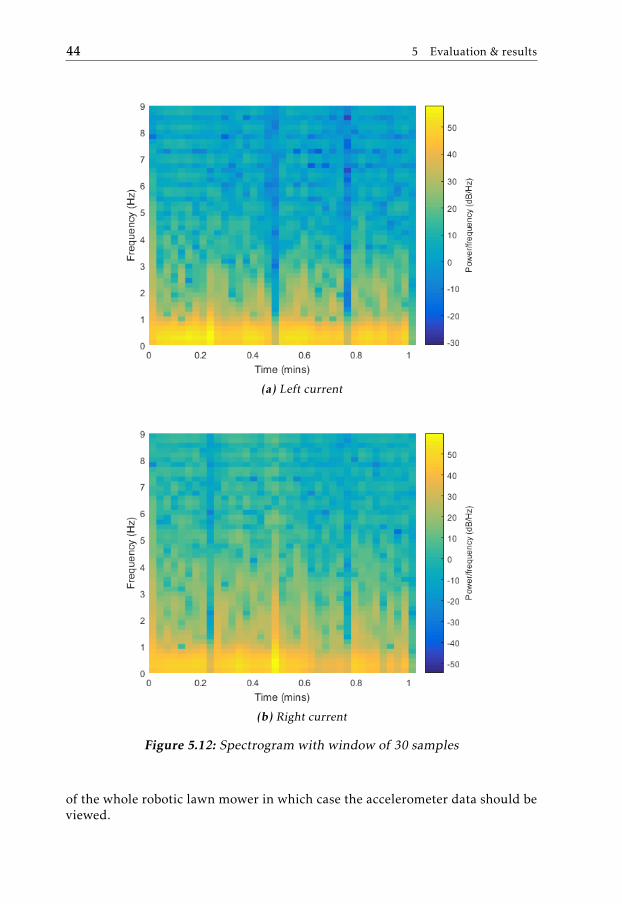
Uneven and rough surface materials give the motor currents a volatile behaviorsince there is a constant change in demand of current to keep a desired speed.When a wheel is lifted the ground surface no longer influence the demand andthus the current should be somewhat constant. The data in Figure 5.9 have a lifton the right hand side around sample 250, on the left hand side around sample500 and the whole robotic lawn mower is lifted around sample 800. The liftscan be seen as a flat part of the signal for that wheel which has been off theground. Consequently higher frequencies should have been damped and onlylow frequencies should dominate. A detection could then either be a lack of highfrequency components or increasing intensity for lower frequencies. The trade offbetween frequency and time resolution then plays an important role. From thedetection perspective a force should be detected as soon as possible and thereforethree different segment sizes have been tested and are shown in Figure 5.10 to5.12. Now the sampling frequency was 18Hz for the currents meaning that thefirst lift around sample 250 would have the approximate time 250/18/60 ≈ 0.23minutes, the left lift would similar have the time ≈ 0.48 and the last lift ≈ 0.75.One can visually make out these areas in the spectrogram graphs but the liftsseems to damp all frequencies and not only higher frequencies. The dampingis however not significant enough thus in order to make this method viable fordetection higher sampling rate would be needed.


(a) Left current

(b) Right current

Figure 5.9: Currents when the robotic lawn mower is lifted on the right sideand left side and whole in that order


(a) Left current

(b) Right current

Figure 5.10: Spectrogram with window of 10 samples

5.2 Standing still 43

(a) Left current

(b) Right current


5.2 Standing still

While standing still all signals should remain constant and a lift would simply bedetected by setting a threshold on the gyroscope data for all cases except for a lift


(a) Left current

(b) Right current


of the whole robotic lawn mower in which case the accelerometer data should beviewed.

5.3 Driving 45

5.3 Driving

The method modeling a pitch current relationship that proved to have fairly goodperformance with current conditions. This method had the most significant devi-ations in its residuals when a front lift and a lift of the whole robotic lawn mowerwas conducted but not as reliable for back and side lifts which means that themethod would need a complimentary detection method. The estimation of globalvelocities could be significantly improved with additional measurements and thefrequency method would need a higher sampling frequency.

6Conclusions

6.1 Summary

Available sensors and proposed methods could not detect all fault cases althougha future complete solution seems plausible.

When the robotic lawn mower is standing still all external forces should be de-tectable by simply using thresholds where a change in any signal would indicatethat an external force is present.

For the odometry method estimates were too poor to be used in constraints onvalid movement meaning that no fault cases could be detected with the method.The primary problem was that estimates are strongly affected by disturbances.With additional ways of measuring either velocity of position the method couldbe significantly improved since more reliable estimation methods such as a Kalmanfilter could be used.

The pitch angle relationship proved to be the best with robust detection for somecases but would need to be complemented for constructing an adequate detec-tion system. This method showed little drawbacks from available sensors mean-ing that the method cannot be improved as much as for instance the odometrymodel.

The frequency method showed too little difference between valid cases and caseswhere external forces where present to provide useful results. Better sensorswith higher sampling frequency might not however make the methods cost effec-tive.

It is the author’s believe that an adequate method can be achieved with a combi-

47

48 6 Conclusions

nation of an improved odometry method and the pitch angle relationship.

6.2 Future work

Improvement of the odometry method could be done with a Kalman filter. Withfor example, some external positioning system a Kalman filter could use accelerom-eter data as input and the position as measurement to produce more accurateestimates. With good estimates the constraints can be used to detect abnormalmovement. Combining the improved odometry method above with the pitch an-gle relationship could result in a complete detection system.

The frequency method has its greatest potential in detecting back wheel lifts.Results would be improved if the sampling frequency was higher but the cost ofbetter sensors might not make the method worth implementing.

Bibliography

[1] Anthony M Block, Jerrold E Marsden, and Zenkov Dmitry V. Nonholonomicdynamics. Norice of the AMS, 52(3):320–329, 2005. Cited on page 7.

[2] Erik Frisk. Residual generation for fault diagnosis, 2001. Cited on pages 23and 24.

[3] Fredrik Gustafsson. Statistical Sensor Fusion. 2010. ISBN 978-91-44-07732.Cited on pages 8, 13, and 27.

[4] Fredrik Gustafsson, Lennart Ljung, and Mille Millnert. Signal Processing.2010. ISBN 978-91-44-05835. Cited on pages 30 and 32.

[5] Layton C Hale. Principles and techniques for desiging precision machines,1999. Cited on page 7.

[6] Boris Ivanic. Användning av accelerometer för detektering av rörelse i husq-varna abs gräsklippare automower. Cited on page 3.

[7] Mikael Olofsson. Signal Theory. Studentlitteratur, 2011. ISBN 978-91-44-073538. Cited on page 23.

[8] Abhinav Parkhi and Mahesh Pawar. Analysis of deformities in lung usingshort time fourier transform spectrogram analysis on lung sound. IEEE,2011. URL http://ieeexplore.ieee.org/stamp/stamp.jsp?tp=&arnumber=6112850. Cited on page 32.

[9] Ken C. Pohlmann. Principles of Digital Audio. McGraw-Hill/TAB Electron-ics, 2005. ISBN 0071441565. Cited on page 25.

[10] Marek Ryćko and Bugosław Jackowski. Determination of initial ca-ble forces in prestressed concrete cable-stayed bridges for givendesign deck pro®les using the force equilibrium method. Com-puters and Structures, 74(1), 2000. URL http://ac.els-cdn.com/S0045794998003150/1-s2.0-S0045794998003150-main.pdf?_tid=276e11c6-654f-11e6-85e8-00000aab0f26&acdnat=

49

http://ieeexplore.ieee.org/stamp/stamp.jsp?tp=&arnumber=6112850

http://ieeexplore.ieee.org/stamp/stamp.jsp?tp=&arnumber=6112850

http://ac.els-cdn.com/S0045794998003150/1-s2.0-S0045794998003150-main.pdf?_tid=276e11c6-654f-11e6-85e8-00000aab0f26&acdnat=1471530312_8f642306e1d8e603b08016b49e5857b9




50 Bibliography

1471530312_8f642306e1d8e603b08016b49e5857b9. Cited on page26.

[11] Angelo Maria Sabatini and Vincenzo Genovese. A sensor fusion methodfor tracking vertical velocity and height based on inertial and barometricaltimeter measurements. Cited on page 3.

[12] Johan Ståhl. Kollisionsdetekteringssystem för autonom robot. LITH-ISY-EX-ET–15/0436–SE, Linköping University, Sweden, 2015. Cited on page 3.



Documents

Detecting external forces on an autonomous lawn …liu.diva-portal.org/smash/get/diva2:1095736/FULLTEXT01.pdf · 1 Introduction 1.1 Background Husqvarna Automower consist of a chassis