Embed Size (px)
Citation preview

Detecting Deception in Speech
Frank Enos
Submitted in partial fulfillment of the
requirements for the degree
of Doctor of Philosophy
in the Graduate School of Arts and Sciences
COLUMBIA UNIVERSITY
2009

c©2009
Frank Enos
All Rights Reserved

ABSTRACT
Detecting Deception in Speech
Frank Enos
This dissertation describes work on the detection of deception in speech using the techniques
of spoken language processing. The accurate detection of deception in human interactions
has long been of interest across a broad array of contexts and has been studied in a number of
fields, including psychology, communication, and law enforcement. The detection of decep-
tion is well-known to be a challenging problem: people are notoriously bad lie detectors,
and no verified approach yet exists that can reliably and consistently catch liars.
To date, the speech signal itself has been largely neglected by researchers as a source of
cues to deception. Prior to the work presented here, no comprehensive attempt has been
made by speech scientists to apply state-of-the-art speech processing techniques to the study
of deception. This work uses a set of features new to the deception domain in classification
experiments, statistical analyses, and speaker- and group-dependent modeling approaches,
all designed to identify and employ potential cues to deception in speech.
This dissertation shows that speech processing techniques are relevant to the deception
domain by demonstrating significant statistical effects for deception on a number of features,
both in corpus-wide and subject-dependent analyses. Results also show that deceptive
speech can be automatically classified with some success: accuracy is better than chance
and considerably better than human hearers performing an analogous task. The work also
examines speaker and group differences with respect to deceptive speech, and we report
a number of findings in this regard. We provide a context for our work via a perception
study in which human hearers attempted to identify deception in our corpus. Through
this perception study we identify a number of previously unreported effects that relate the
personality of the hearer to deception detection ability. An additional product of this work
is the CSC Corpus, a new corpus of deceptive speech.

Contents
I Preliminaries 1
1 Introduction 2
1.1 Goal . . . . . . . . . . . . . . . . . . . . . . . . . . . . . . . . . . . . . . . . . 3
1.2 Scope . . . . . . . . . . . . . . . . . . . . . . . . . . . . . . . . . . . . . . . . 4
1.3 Approach . . . . . . . . . . . . . . . . . . . . . . . . . . . . . . . . . . . . . . 5
2 Previous Research on Deception 6
2.1 Theory . . . . . . . . . . . . . . . . . . . . . . . . . . . . . . . . . . . . . . . . 7
2.2 Empirical Studies of Deceptive Speech . . . . . . . . . . . . . . . . . . . . . . 9
2.3 Detection Technologies . . . . . . . . . . . . . . . . . . . . . . . . . . . . . . . 9
2.4 Previous Work on Individual Differences in Deception . . . . . . . . . . . . . 11
2.4.1 Individual differences and non-verbal cues . . . . . . . . . . . . . . . . 11
2.4.2 Individual differences and speech cues . . . . . . . . . . . . . . . . . . 14
2.5 Perception Studies . . . . . . . . . . . . . . . . . . . . . . . . . . . . . . . . . 15
2.6 Conclusions . . . . . . . . . . . . . . . . . . . . . . . . . . . . . . . . . . . . . 17
3 Columbia-SRI-Colorado (CSC) Corpus 18
3.1 Rationale for collecting . . . . . . . . . . . . . . . . . . . . . . . . . . . . . . . 19
3.2 The corpus . . . . . . . . . . . . . . . . . . . . . . . . . . . . . . . . . . . . . 20
3.2.1 Method . . . . . . . . . . . . . . . . . . . . . . . . . . . . . . . . . . . 20
3.2.2 Example dialogs . . . . . . . . . . . . . . . . . . . . . . . . . . . . . . 25
3.2.3 Recording and labeling . . . . . . . . . . . . . . . . . . . . . . . . . . . 28
3.3 Feature extraction . . . . . . . . . . . . . . . . . . . . . . . . . . . . . . . . . 28
i

3.3.1 Acoustic and prosodic features . . . . . . . . . . . . . . . . . . . . . . 29
3.3.2 Lexical features . . . . . . . . . . . . . . . . . . . . . . . . . . . . . . . 30
3.3.3 Subject-dependent features . . . . . . . . . . . . . . . . . . . . . . . . 32
3.4 Discussion . . . . . . . . . . . . . . . . . . . . . . . . . . . . . . . . . . . . . . 33
II General Analysis and Classification 35
4 Statistical Analysis 36
4.1 Statistical Methods . . . . . . . . . . . . . . . . . . . . . . . . . . . . . . . . . 36
4.2 Binary Lexical Features . . . . . . . . . . . . . . . . . . . . . . . . . . . . . . 38
4.3 Numerical Features . . . . . . . . . . . . . . . . . . . . . . . . . . . . . . . . . 40
4.3.1 Results and discussion . . . . . . . . . . . . . . . . . . . . . . . . . . . 42
4.4 Conclusions . . . . . . . . . . . . . . . . . . . . . . . . . . . . . . . . . . . . . 46
5 Analysis and Classification on the Local Level 50
5.1 Preliminary Analyses . . . . . . . . . . . . . . . . . . . . . . . . . . . . . . . . 50
5.2 Preliminary Local Lie Classification With Ripper . . . . . . . . . . . . . . . . 52
5.3 Local Lie Classification Using Combined Classifiers . . . . . . . . . . . . . . . 53
5.3.1 Data . . . . . . . . . . . . . . . . . . . . . . . . . . . . . . . . . . . . . 54
5.3.2 Prosodic-lexical SVM system . . . . . . . . . . . . . . . . . . . . . . . 54
5.3.3 Acoustic GMM system . . . . . . . . . . . . . . . . . . . . . . . . . . . 55
5.3.4 Combiner SVM system . . . . . . . . . . . . . . . . . . . . . . . . . . . 55
5.3.4.1 Results . . . . . . . . . . . . . . . . . . . . . . . . . . . . . . 56
5.3.5 Prosodic System from Recognized Words . . . . . . . . . . . . . . . . . 57
5.4 In-depth Machine Learning Experiments . . . . . . . . . . . . . . . . . . . . . 57
5.4.1 Performance Metrics . . . . . . . . . . . . . . . . . . . . . . . . . . . . 60
5.4.2 The Base feature set . . . . . . . . . . . . . . . . . . . . . . . . . . . . 61
5.4.3 The Base + Subject-dependent feature set . . . . . . . . . . . . . . . . 63
5.4.4 The All feature set . . . . . . . . . . . . . . . . . . . . . . . . . . . . . 65
ii

5.4.5 The Best 39 feature set . . . . . . . . . . . . . . . . . . . . . . . . . . 65
5.4.6 Discussion . . . . . . . . . . . . . . . . . . . . . . . . . . . . . . . . . . 69
5.5 Conclusions . . . . . . . . . . . . . . . . . . . . . . . . . . . . . . . . . . . . . 71
6 Classification of Global Lies 73
6.1 Global Lies Via Critical Segments . . . . . . . . . . . . . . . . . . . . . . . . 74
6.2 Methods and Materials . . . . . . . . . . . . . . . . . . . . . . . . . . . . . . . 75
6.2.1 Selection of critical segments . . . . . . . . . . . . . . . . . . . . . . . 75
6.2.2 Coping with skewed class distributions . . . . . . . . . . . . . . . . . . 76
6.3 Results and Discussion . . . . . . . . . . . . . . . . . . . . . . . . . . . . . . . 77
6.3.1 Relevant features . . . . . . . . . . . . . . . . . . . . . . . . . . . . . . 79
6.3.2 Other observations . . . . . . . . . . . . . . . . . . . . . . . . . . . . . 81
6.4 Conclusions and Future Work . . . . . . . . . . . . . . . . . . . . . . . . . . . 82
III Speaker and Group Dependent Analyses 84
7 Motivations 85
7.1 Previous Work . . . . . . . . . . . . . . . . . . . . . . . . . . . . . . . . . . . 86
7.2 Exploratory Analyses . . . . . . . . . . . . . . . . . . . . . . . . . . . . . . . . 86
7.2.1 Methods . . . . . . . . . . . . . . . . . . . . . . . . . . . . . . . . . . . 87
7.2.2 Observations . . . . . . . . . . . . . . . . . . . . . . . . . . . . . . . . 87
8 Speaker-Dependent Statistical Analyses 91
8.1 Statistical Methods . . . . . . . . . . . . . . . . . . . . . . . . . . . . . . . . . 91
8.2 Results on Binary Features . . . . . . . . . . . . . . . . . . . . . . . . . . . . 93
8.2.1 Discussion . . . . . . . . . . . . . . . . . . . . . . . . . . . . . . . . . . 95
8.3 Results on Numeric Features . . . . . . . . . . . . . . . . . . . . . . . . . . . 99
8.3.1 Discussion of feature classes . . . . . . . . . . . . . . . . . . . . . . . . 113
8.3.2 Towards a visualization of speaking styles . . . . . . . . . . . . . . . . 119
iii

8.4 Conclusions . . . . . . . . . . . . . . . . . . . . . . . . . . . . . . . . . . . . . 123
9 Group and Subject Dependent Modeling 125
9.1 Subjects Grouped by Gender . . . . . . . . . . . . . . . . . . . . . . . . . . . 125
9.2 Subjects Grouped by Graph-derived Clusters . . . . . . . . . . . . . . . . . . 130
9.3 Another Approach to Speaker Similarity . . . . . . . . . . . . . . . . . . . . . 135
9.3.1 Discussion . . . . . . . . . . . . . . . . . . . . . . . . . . . . . . . . . . 137
9.4 Speaker-dependent Models . . . . . . . . . . . . . . . . . . . . . . . . . . . . . 138
9.5 Conclusions and Future Work . . . . . . . . . . . . . . . . . . . . . . . . . . . 140
IV Human Deception Detection 144
10 Human Deception Detection and the CSC Corpus 145
10.1 Previous Research . . . . . . . . . . . . . . . . . . . . . . . . . . . . . . . . . 145
10.2 Procedure . . . . . . . . . . . . . . . . . . . . . . . . . . . . . . . . . . . . . . 146
10.3 Results on Deception Detection . . . . . . . . . . . . . . . . . . . . . . . . . . 148
10.3.1 Additional findings . . . . . . . . . . . . . . . . . . . . . . . . . . . . . 149
10.4 Predicting Detectability of the Speaker . . . . . . . . . . . . . . . . . . . . . . 157
10.4.1 Materials and methods . . . . . . . . . . . . . . . . . . . . . . . . . . . 159
10.4.2 Three-class prediction . . . . . . . . . . . . . . . . . . . . . . . . . . . 160
10.4.3 Two-class prediction . . . . . . . . . . . . . . . . . . . . . . . . . . . . 161
10.4.4 Discussion . . . . . . . . . . . . . . . . . . . . . . . . . . . . . . . . . . 162
10.5 The Personality of the Hearer: Effects on Performance . . . . . . . . . . . . . 166
10.5.1 Materials and methods . . . . . . . . . . . . . . . . . . . . . . . . . . . 166
10.5.2 Results . . . . . . . . . . . . . . . . . . . . . . . . . . . . . . . . . . . 168
10.6 Conclusions . . . . . . . . . . . . . . . . . . . . . . . . . . . . . . . . . . . . . 175
iv

V Conclusions 176
11 Conclusions 177
11.1 Summary of Findings . . . . . . . . . . . . . . . . . . . . . . . . . . . . . . . . 178
11.1.1 Statistical Analyses . . . . . . . . . . . . . . . . . . . . . . . . . . . . . 178
11.1.1.1 Binary lexical features . . . . . . . . . . . . . . . . . . . . . . 178
11.1.1.2 Numerical features . . . . . . . . . . . . . . . . . . . . . . . . 179
11.1.2 Classification of local lies . . . . . . . . . . . . . . . . . . . . . . . . . 180
11.1.3 Classification of global lies . . . . . . . . . . . . . . . . . . . . . . . . . 181
11.1.4 Speaker dependent analyses . . . . . . . . . . . . . . . . . . . . . . . . 182
11.1.4.1 Binary features . . . . . . . . . . . . . . . . . . . . . . . . . . 182
11.1.4.2 Numeric Features . . . . . . . . . . . . . . . . . . . . . . . . 183
11.1.5 Group dependent classification . . . . . . . . . . . . . . . . . . . . . . 184
11.1.6 Human performance at classifying the CSC Corpus . . . . . . . . . . . 184
11.2 Contributions . . . . . . . . . . . . . . . . . . . . . . . . . . . . . . . . . . . . 185
11.3 Implications for Practitioners . . . . . . . . . . . . . . . . . . . . . . . . . . . 185
11.4 Future Work . . . . . . . . . . . . . . . . . . . . . . . . . . . . . . . . . . . . 186
VI Bibliography 188
Bibliography 189
VII Appendices 198
A Protocol 199
A.1 Subject Introduction . . . . . . . . . . . . . . . . . . . . . . . . . . . . . . . . 199
A.1.1 Biographical Questions . . . . . . . . . . . . . . . . . . . . . . . . . . . 199
A.2 Tasks . . . . . . . . . . . . . . . . . . . . . . . . . . . . . . . . . . . . . . . . 199
A.3 Interview Instructions . . . . . . . . . . . . . . . . . . . . . . . . . . . . . . . 200
v
A.3.1 Scores . . . . . . . . . . . . . . . . . . . . . . . . . . . . . . . . . . . . 200
A.3.2 Interview Process . . . . . . . . . . . . . . . . . . . . . . . . . . . . . . 201
A.3.3 Interview Preparation . . . . . . . . . . . . . . . . . . . . . . . . . . . 202
A.4 Debriefing . . . . . . . . . . . . . . . . . . . . . . . . . . . . . . . . . . . . . . 202
A.5 Biographical Questionnaire . . . . . . . . . . . . . . . . . . . . . . . . . . . . 203
B Pre-test Questions 205
B.1 Interactive Tasks . . . . . . . . . . . . . . . . . . . . . . . . . . . . . . . . . . 205
B.1.1 Easy . . . . . . . . . . . . . . . . . . . . . . . . . . . . . . . . . . . . . 205
B.1.2 Difficult . . . . . . . . . . . . . . . . . . . . . . . . . . . . . . . . . . . 206
B.2 Musical . . . . . . . . . . . . . . . . . . . . . . . . . . . . . . . . . . . . . . . 210
B.2.1 Easy . . . . . . . . . . . . . . . . . . . . . . . . . . . . . . . . . . . . . 210
B.2.2 Difficult . . . . . . . . . . . . . . . . . . . . . . . . . . . . . . . . . . . 210
B.3 Survival / first aid (easy and difficult) . . . . . . . . . . . . . . . . . . . . . . 210
B.4 Food and Wine Knowledge . . . . . . . . . . . . . . . . . . . . . . . . . . . . 211
B.4.1 Easy . . . . . . . . . . . . . . . . . . . . . . . . . . . . . . . . . . . . . 211
B.4.2 Difficult . . . . . . . . . . . . . . . . . . . . . . . . . . . . . . . . . . . 211
B.5 Geography of New York City . . . . . . . . . . . . . . . . . . . . . . . . . . . 212
B.5.1 Easy . . . . . . . . . . . . . . . . . . . . . . . . . . . . . . . . . . . . . 212
B.5.2 Difficult . . . . . . . . . . . . . . . . . . . . . . . . . . . . . . . . . . . 212
B.6 Civics . . . . . . . . . . . . . . . . . . . . . . . . . . . . . . . . . . . . . . . . 213
B.6.1 Easy . . . . . . . . . . . . . . . . . . . . . . . . . . . . . . . . . . . . . 213
B.6.2 Difficult . . . . . . . . . . . . . . . . . . . . . . . . . . . . . . . . . . . 213
C Features 214
C.1 Notes . . . . . . . . . . . . . . . . . . . . . . . . . . . . . . . . . . . . . . . . 215
vi

List of Figures
3.1 Photograph of the Interview Setting . . . . . . . . . . . . . . . . . . . . . . . 21
4.1 Boxplots of significant numerical features: 1 . . . . . . . . . . . . . . . . . . . 47
4.2 Boxplots of significant numerical features: 2 . . . . . . . . . . . . . . . . . . . 48
4.3 Boxplots of significant numerical features: 3 . . . . . . . . . . . . . . . . . . . 49
5.1 Local Lie Performance: Base Features . . . . . . . . . . . . . . . . . . . . . . 62
5.2 Local Lie Performance: Base + Subject-dependent Features . . . . . . . . . . 64
5.3 Local Lie Performance: All Features . . . . . . . . . . . . . . . . . . . . . . . 66
5.4 Local Lie Performance: 39 Features from Base + Subject-dependent . . . . . 69
5.5 Local Lie Performance: Best Learners for Feature Sets . . . . . . . . . . . . . 71
7.1 Counts of Significant Logistic Regression Coefficients . . . . . . . . . . . . . . 88
8.1 Counts by subject, p≤ 0.01 . . . . . . . . . . . . . . . . . . . . . . . . . . . . 101
8.2 Counts by subject, ≤ 0.05 . . . . . . . . . . . . . . . . . . . . . . . . . . . . . 102
8.3 Counts by feature, p≤ 0.01 . . . . . . . . . . . . . . . . . . . . . . . . . . . . 103
8.4 Counts by feature, ≤ 0.05 . . . . . . . . . . . . . . . . . . . . . . . . . . . . . 104
8.5 Numerical features by test and subject . . . . . . . . . . . . . . . . . . . . . . 111
8.6 Numerical features by test and feature . . . . . . . . . . . . . . . . . . . . . . 112
8.7 Significant numerical features with categories . . . . . . . . . . . . . . . . . . 114
8.8 Significant numerical features with categories, cont. . . . . . . . . . . . . . . . 115
8.9 Graph of subjects related by features . . . . . . . . . . . . . . . . . . . . . . . 120
vii

9.1 Local Lie Performance: Grouped by Gender . . . . . . . . . . . . . . . . . . . 130
9.2 Local Lie Performance: Grouped by Cluster . . . . . . . . . . . . . . . . . . . 132
9.3 Local Lie Relative Accuracy . . . . . . . . . . . . . . . . . . . . . . . . . . . . 142
9.4 Local Lie F-measure . . . . . . . . . . . . . . . . . . . . . . . . . . . . . . . . 143
10.1 Histograms of Judge Confidence . . . . . . . . . . . . . . . . . . . . . . . . . . 151
10.2 Plot of Judge Performance vs. Number of Significant Features . . . . . . . . . 157
10.3 Graph of Speakers Related by Features . . . . . . . . . . . . . . . . . . . . . . 158
10.4 Plot of Judge Performance, Sorted . . . . . . . . . . . . . . . . . . . . . . . . 159
10.5 Speakers Labeled for Detectability, Two Classes (A) . . . . . . . . . . . . . . 161
10.6 Speakers Labeled for Detectability, Two Classes (B) . . . . . . . . . . . . . . . 161
10.7 Plot of Detectability Classification Hits and Misses . . . . . . . . . . . . . . . 163
10.8 Plots of Regression Models . . . . . . . . . . . . . . . . . . . . . . . . . . . . . 172
10.9 Personality Scores of Best and Worst Performing Subjects . . . . . . . . . . . 174
viii

List of Tables
2.1 Linguistic and Paralinguistic Cues to Deception (DePaulo et al., 2003) . . . . 10
2.2 Detection Accuracy of Various Groups . . . . . . . . . . . . . . . . . . . . . . 16
3.1 Subject Statistics . . . . . . . . . . . . . . . . . . . . . . . . . . . . . . . . . . 23
4.1 Binary Lexical Features by Subject . . . . . . . . . . . . . . . . . . . . . . . . 39
4.2 Numeric Feature Key . . . . . . . . . . . . . . . . . . . . . . . . . . . . . . . . 41
4.3 Analysis of Base Numerical Features . . . . . . . . . . . . . . . . . . . . . . . 43
5.1 Accuracy of Single Systems and Combination Systems on the CSC Corpus
(Graciarena et al., 2006). . . . . . . . . . . . . . . . . . . . . . . . . . . . . . . 56
5.2 Human Transcribed vs. Recognized Prosodic Systems. (Graciarena et al.,
2006). . . . . . . . . . . . . . . . . . . . . . . . . . . . . . . . . . . . . . . . . 57
5.3 Local Lie Performance: Base Features . . . . . . . . . . . . . . . . . . . . . . 62
5.4 Local Lie Performance: Base + Subject-dependent Features . . . . . . . . . . 63
5.5 Local Lie Performance: All Features . . . . . . . . . . . . . . . . . . . . . . . 65
5.6 Best 39 Feature Set . . . . . . . . . . . . . . . . . . . . . . . . . . . . . . . . . 67
5.7 Local Lie Performance: 39 Features from Base + Subject-dependent . . . . . 68
5.8 Local Lie Performance: Best Learners for Feature Sets . . . . . . . . . . . . . 69
6.1 Accuracy Detecting Global Lies . . . . . . . . . . . . . . . . . . . . . . . . . . 78
6.2 Features Used in Classifying the Critical-Plus data set . . . . . . . . . . . . . 80
6.3 Features Used in Classifying the Critical Dataset . . . . . . . . . . . . . . . . 81
ix

7.1 Logistic Regression Coefficients . . . . . . . . . . . . . . . . . . . . . . . . . . 89
8.1 Significance of Binary Lexical Features . . . . . . . . . . . . . . . . . . . . . . 94
8.2 Significant Binary Features, Counts by Feature . . . . . . . . . . . . . . . . . 96
8.3 Significant Binary Features, Counts by Subject . . . . . . . . . . . . . . . . . 97
8.4 Numeric Feature Key . . . . . . . . . . . . . . . . . . . . . . . . . . . . . . . . 100
8.5 Numeric Features Significant at the 0.01 Level. . . . . . . . . . . . . . . . . . 106
8.6 Numeric Features Significant at the 0.05 Level . . . . . . . . . . . . . . . . . . 108
9.1 Best 39 Feature Set . . . . . . . . . . . . . . . . . . . . . . . . . . . . . . . . . 127
9.2 Custom Feature Sets: Female and Male Groups . . . . . . . . . . . . . . . . . 128
9.3 Local Lie Performance: Grouped by Gender . . . . . . . . . . . . . . . . . . . 129
9.4 Local Lie Performance: Grouped by Cluster . . . . . . . . . . . . . . . . . . . 131
9.5 Custom Feature Set: Cluster A . . . . . . . . . . . . . . . . . . . . . . . . . . 133
9.6 Custom Feature Set: Cluster B . . . . . . . . . . . . . . . . . . . . . . . . . . 134
9.7 c4.5 Performance on Grouped Speakers . . . . . . . . . . . . . . . . . . . . . . 136
9.8 Local Lie Performance on Single Speakers . . . . . . . . . . . . . . . . . . . . 138
10.1 Judges’ Aggregate Performance . . . . . . . . . . . . . . . . . . . . . . . . . . 148
10.2 Aggregate Performance by Speaker . . . . . . . . . . . . . . . . . . . . . . . . 149
10.3 Global Lie Performance by Judge . . . . . . . . . . . . . . . . . . . . . . . . . 153
10.4 Global Lie Performance by Speaker . . . . . . . . . . . . . . . . . . . . . . . . 154
10.5 Local Lie Performance by Judge . . . . . . . . . . . . . . . . . . . . . . . . . . 155
10.6 Local Lie Performance by Speaker . . . . . . . . . . . . . . . . . . . . . . . . 156
10.7 Detectability Classification Accuracy . . . . . . . . . . . . . . . . . . . . . . . 163
10.8 Feature Sets Used in Predicting Detectability . . . . . . . . . . . . . . . . . . 165
10.9 Correlations: Personality Factors and Performance . . . . . . . . . . . . . . . 169
10.10 Personality Factors Predict Judge Performance . . . . . . . . . . . . . . . . . 170
C.1 Feature Descriptions . . . . . . . . . . . . . . . . . . . . . . . . . . . . . . . . 216
x

Acknowledgments
This should, in fairness, be the longest chapter.
I am extraordinarily indebted to Julia Hirschberg for taking a chance on a guy with no
formal qualifications beyond a music degree and an Actors’ Equity union card. From the
very beginning, this has been a wonderful experience for me, and I have profited from her
knowledge, wisdom, patience, generosity, confidence, and great humanity. And in the times
when finishing seemed most impossible, I always reminded myself that she did it twice. For
all of this, I am very grateful.
My dissertation committee — Dan Ellis, Kathleen McKeown, Owen Rambow, and
Elizabeth Shriberg — have been helpful, patient, and generous throughout this process
as well, and I feel honored that they have invested their time and efforts in this project.
This work bears the deep imprint of their assistance, both direct and indirect, as I have
learned from them over the years in various ways.
The work reported here has been a large project with many participants. The original
team consisted of Stefan Benus, Jason M. Brenier, Sarah Friedman, Sarah Gilman, Cynthia
Girand, Martín Graciarena, Julia Hirschberg, Andreas Kathol, Laura Michaelis and Jennifer
Venditti-Ramprashad. I profited from the help of all of these people, and from the good
fortune of finding myself on such a fine team. Laura Davies, Jean-Philippe Goldman, Jared
Kennedy, Kadri Hacioglu, Max Shevyakov, and Wayne Thorsen also participated. I’m
especially grateful to Jason M. Brenier and Cynthia Griand, who carried out some of the
early analyses; to Sarah Friedman, who worked on the lexical features; and to Sarah Gilman,
who ran the early experiments. Robin Cautin helped to design and analyze the perception
study, and provided statistical and methodological advice throughout this work. I am of
course grateful to the anonymous subjects who participated in both studies we conducted.
I am especially indebted to Stefan Benus for his tireless involvement in the perception
xi

work as a whole, as it would not exist without his efforts. He also carried out the bulk of
the work on the analysis of pauses and has continued to offer advice on this work. Martín
Graciarena has been extremely generous with his time and knowledge, and was responsible
for extracting the acoustic and prosodic features, most of the work on combined classifiers,
and countless other tasks as well. Elizabeth Shriberg has been involved with literally every
aspect of my work on this project. She has provided insight, support, and sanity checks at
crucial times in this process, and in particular contributed a great deal to the design of both
paradigms, to the work on global lies, and the work on group and individual differences.
I’ve had many helpful conversations with Maureen O’Sullivan and Jeffrey Cohn, and
Michael Aamodt has been generous with his work and results. Frederick Frese was generous
in sharing his findings and in helping me to obtain a copy of his dissertation.
At Columbia, Jonathan Gross took me seriously from the beginning, and offered en-
couragement and advice that made this seem possible; along the way he taught me a lot of
mathematics as well. I am forever indebted to Christina Leslie for her early encouragement,
for being such an engaging teacher, and for having introduced me to Julia Hirschberg.
Fadi Biadsy, Stefan Benus, Sasha Caskey, Bob Coyne, Agustín Gravano, Martin Jansche,
Jackson Liscombe, Sameer Maskey, Andrew Rosenberg and Jennifer Venditti have made up
the Speech Lab, and have been invaluable colleagues. My family and I are particularly
grateful to Agus and Fadi for having repeatedly covered my duties in the lab as family
obligations arose. I’m grateful to Andrew for years of technical advice and good humor, and
to Jackson for moral support and helpful conversations about our shared interests. Martin
Jansche gave me some form of advice on almost everything I did during his time in the lab.
Dave Elson, Ani Nenkova, and Barry Schiff of the NLP Group provided early assistance
with the project, and Ani and Barry both provided helpful advice about how to finish.
I am grateful for the support of wonderful friends. Scott Brinker has shared his contagious
enthusiasm for learning, his tremendous insight on all manner of topics, and what can only
be termed great esprit de corps in the face of challenges. Elizabeth and Michael Gallo
and David Diehl and Katya Mia Nicolai were wonderful supports from the very beginning,
xii

and I’ve been grateful for the encouragement of Alex Shakow. Ludy T. Benjamin Jr. has
provided sound advice along the way about how to finish, and he and Priscilla Benjamin
have offered welcome moral support to me and my family. Valerie Smith has been a great
support in this undertaking, and generously proofread some of this manuscript.
The persistent support of John Daido Loori, Geoffrey Shugen Arnold, Konrad Ryushin
Marchaj, Jody Hojin Kimmel, and Thayer Kyusan Case has been invaluable to me.
My work has benefited enormously from what I learned from Stephen Berenson and
Brian McEleney at Trinity Rep Conservatory, and from studying singing with Phyllis Curtin.
John Cavanaugh and J. Tom Williams helped me early on to recognize and explore my love
of science and of language.
I am grateful to Joe Chanin, Richard Patrick-Sternin, and Tom Vincent for having hired
me to do work that led, circuitously, to this undertaking.
Kathy McKeown has provided continual support and encouragement, and sound advice
on how to negotiate all of this while starting a family.
I am grateful to my family. David Cautin and Alison Yaffie have provided moral support,
sound advice, well-timed meals and welcome hospitality throughout. I could not begin to
express in a few lines how grateful I am to Barbara and Harvey Cautin for their love and
logistical, moral, material, and technical support. We could never have done this without
them. I am profoundly grateful to my parents Antoinette and Frank for convincing me that I
could do anything I wanted to do, and for never questioning any of my unlikely undertakings,
except to ask how they could help.
My wife, Robin Cautin, in addition to being a wonderful collaborator, has provided love,
support, technical and personal advice, help of every kind, and the invaluable certainty that
I could do this. Without her I would likely have never undertaken this process; I certainly
would not have succeeded. Robin and I are grateful to Fletcher for comic relief, and I am
very, very grateful to Ben and Maddie for having been so brave through all of this.
This research was supported by grants from the National Science Foundation (NSF IIS-
0325399) and the Department of Homeland Security.
xiii

For Robin, Benjamin, and Madeleine, who made the sacrifices that made this possible.
xiv

PART I. 1
Part I
Preliminaries

Chapter 1. 2
Chapter 1
Introduction
The accurate detection of deception in human interactions has long been of interest across a
broad array of contexts and disciplines. It holds obvious relevance for the realms of business,
politics, jurisprudence, law enforcement, and national security. This topic also enjoys strong
interest in the field of psychology, as well as in the literature of popular psychology; this
latter is likely representative of the fascination deception engenders in the public at large.
Considerable work relating to deception has been undertaken in fields such as psychology,
communication, and to some extent, law enforcement. The bulk of that work has focused
on gestural and facial cues to deception. Limited work has been done with the aim of devel-
oping scientifically verified automatic deception detection, and even less work has focused
specifically on speech. The present work represents the first comprehensive attempt to apply
a broad array of techniques from spoken language processing to the tasks of detecting de-
ception in speech, and to identifying acoustic, lexical, prosodic and paralinguistic correlates
of deception.
The speech signal has been relatively neglected in existing research as a source of cues to
deception. Nevertheless, we show here in work using a corpus collected for this project — the
Columbia-SRI-Colorado (CSC) Corpus of Deceptive Speech (Chapter 3) — that it is possible
to classify deceptive speech automatically more accurately than chance and markedly better
than human listeners. (Human judges actually performed worse than chance at detecting
deception on the CSC Corpus, as we will detail in Chapter 10.) One obstacle to research in
this area is that it is difficult to design and collect corpora of deceptive behavior — speech

CHAPTER 1. INTRODUCTION 3
or otherwise — in a manner that is both ethically acceptable and experimentally sound
with respect to the salient components of a deceptive interaction. The work presented here
represents the design and collection of such a corpus.
1.1 Goal
The goal of this work is to examine the efficacy of applying state-of-the art speech processing
techniques to the problem of deceptive speech. In particular we have sought to demonstrate
this efficacy through statistical analyses and classification experiments using a large number
of features and methods that have not previously been applied to this domain. We hoped
to show that such techniques could provide insights about deceptive speech behavior, and
in the best case, could be employed to classify deceptive speech better than chance and
better than human listeners; we have been moderately successful in both these regards.
Deception detection is an unusual problem in the speech processing domain in that humans
perform very poorly at the task. Thus, while matching human performance would represent
considerable success in the speech recognition, speech-to speech-translation, or even emotion
detection domains, we will show both in our literature review and in our own perception
study that humans generally perform near chance — or worse — at deception detection. In
this first work, therefore, we did not set out to create an end-to-end solution to the deceptive
speech detection problem, and we make no claims that this work represents such a solution.
In the present work there are five main research objectives:
1. To design and collect a corpus of deceptive speech in which speakers are motivated to
deceive and for which ground truth is known, of sufficiently high recording quality to
allow for the extraction of a wide variety of acoustic, prosodic, paralinguistic, lexical,
and discourse features.
2. To identify acoustic, prosodic, lexical, and other correlates of deceptive speech.
3. To examine the feasibility of automatic detection of deceptive speech, and to create
machine learning models that can perform such detection with accuracy exceeding
chance and human performance.

CHAPTER 1. INTRODUCTION 4
4. To examine the impact of individual and group differences on deceptive speech.
5. To investigate human ability to detect deception in speech, both for the merit of doing
so and for the purpose of providing context for our automated classification approaches.
1.2 Scope
For the purposes of this work, we employ DePaulo’s (DePaulo, Lindsay, Malone, Muhlen-
bruck, Charlton & Cooper, 2003) definition of deception: “a deliberate attempt to mislead
others”. This definition excludes self-deception and error. We use the terms deception, deceit,
and lying interchangeably in this dissertation.
Because a limited amount of work on deception has previously been carried out in the
field of speech processing, this dissertation could address a great many potential questions.
We have, by necessity narrowed the scope of our work in several ways. First, as we will
describe in detail, we make a distinction between veracity with respect to the propositional
content of individual segments and veracity with respect to the overall attempt to deceive
with regard to salient topics of the discourse. These two categories of course overlap, and we
have examined both, but the bulk of the work presented here focuses on the propositional
content of subject utterances. Second, as we will also describe, there are a number of
possible segmentations of the speech corpus we collected, ranging from individual words to
entire sections of the interview conducted. For the most part this work focuses on sentence-
like units (EARS SLASH-UNITS or SUs (NIST, 2004)). We do this because all of our
lexical and discourse features are linguistically meaningful at this level of granularity, and
at the same time the unit is small enough that our acoustic — and particularly prosodic —
features are theoretically meaningful as well. Use of this segmentation has the added merit
of avoiding the inflation of significance in our statistical analyses, since the class labels of
the smaller units are of course dependent within a given SU. We also focus on this unit for
the pragmatic reason that attempting to apply all analyses to all segmentation levels would
have resulted in a combinatorial explosion of the scope of our work.

CHAPTER 1. INTRODUCTION 5
1.3 Approach
To fulfill our objectives, we have engaged in the following research activities:
• The design and collection of the CSC Corpus of deceptive speech.
• An examination of deceptive behavior in speech at several theoretically motivated
levels of analysis:
– Statistical analyses and identification of correlates to deception.
– Experiments in the detection of deception in terms of the propositional content
of segments.
– Experiments in the detection of deception in terms of the speaker’s intention to
deceive with respect to overall topics of the discourse.
– Experiments in modeling deception with respect to individual speakers and groups
of speakers that share common characteristics.
• Experiments examining the ability of humans to detect deception in the CSC Corpus.
In the first section of this dissertation, we describe previous work and other preliminaries,
and then introduce the CSC Corpus of deceptive speech. In the second section we report
statistical analyses and classification experiments that combine the data of all subjects
in the corpus. In the third section, we report on analyses and classification performed on
individual subjects and groups of subjects that were aggregated via any of several principled
approaches. In the fourth section we report a perception study that engaged human listeners
to attempt to detect deception in the CSC Corpus. In the final section we offer concluding
remarks and suggestions for future research.
We hope that the work reported here, in addition to having its own merit, may offer
guidance on approaches to future work that applies speech processing techniques to the
deception detection domain.

Chapter 2. 6
Chapter 2
Previous Research on Deception
Humans are notoriously poor at detecting deception. A 2006 meta-analysis (C. F. Bond &
DePaulo, 2006) shows that, on average, subjects in 206 studies perform near chance. This
means that, should automatically extractable cues to deception exist (and a number of such
cues are identified in the work presented here), the goal of an automatic detection detection
system would be to perform substantially better than the average human. This places
deception detection in stark contrast with other speech processing tasks, such as speech-to-
speech translation or emotion detection, where human performance is often considered the
gold standard.
A substantial amount of work in the psychology literature examines facial, physiological,
and gestural cues to deception (see (DePaulo, Lindsay, Malone, Muhlenbruck, Charlton &
Cooper, 2003) for an overview of work on human-perceptible cues). Work on detecting
deception through behavioral and physiological cues appears in law enforcement literature,
and such work also appears in communication journals (e.g. (Burgoon, 1996)). In this
section, we will briefly describe three classes of existing work on deception: theoretical,
empirical, and efforts to develop deception detection technologies.
Interest in deception detection is ancient; an early reference to cues to deception, specific
to the questioning of suspected poisoners, appears in the Vedas:
A person who gives poison may be recognized. He does not answer questions,
or they are evasive answers; he speaks nonsense, rubs the great toe along the

CHAPTER 2. PREVIOUS RESEARCH ON DECEPTION 7
ground, and shivers; his face is discolored; he rubs the roots of the hair with his
fingers; and he tries by every means to leave the house... ((Wise, 1860), as cited
in (Trovillo, 1939a))
Trovillo (1939a, 1939b) makes a fascinating, if slightly sensational, account of the history
of deception detection. His history includes “The Method of the Ordeal” (tests of veracity
involving the ability to endure unscathed, for example, contact of the tongue with red-hot
iron); early measures of pulse and blood pressure dating as early as ca. 250 BCE; and an
early history of the polygraph.
2.1 Theory
A number of theoretical treatises exist on the phenomena of lying and deception. By far
the most influential and most often cited is that of psychologist Paul Ekman (2001), now
in its second edition. Among extant theoretical work, Ekman’s is also the most developed
with respect to the task of detecting deception; other work tends to focus broadly on the
motivations for deceiving, or the phenomena of self-deception or pathologically motivated
deception.
Ekman offers a reasoned theory of strategies for deception: concealment, falsification,
misdirection, and several more rarefied strategies, many with ample anecdotal examples.
His approach to detecting deception is based on the theory that cues to deception result
from one of two flaws: leakage (most simply, part of the truth is exposed), or deception
clues (direct indications that the speaker is deceiving, such as inconsistencies in a story).
These basic ideas are supported by the description of the impact of cognitive load (e.g.
“bad lines”) and the emotional effects of lying, specifically fear, guilt, and what Ekman calls
“duping delight”. In the process of developing his substantial theory, Ekman considers in
detail the implications of his ideas with respect to lexical and prosodic components of speech,
physical behavior, and especially, facial expressions. He describes in detail the sorts of facial
expressions that he regards as symptomatic of deception, and the contexts in which they
are found. He also describes in some detail what he holds to be common misconceptions
with regard to deception, emphasizing in particular that there exists no “Pinocchio effect”,

CHAPTER 2. PREVIOUS RESEARCH ON DECEPTION 8
(Vrij, 2004) that is, a universal indicator of deception that is reliable across all subjects in
all contexts.
Ekman’s work is important not only because it represents a comprehensive theory of
deception, but also because he is held in such high regard by law enforcement, intelligence,
and other practitioners, many of whom have had some exposure to the work of Ekman or
his associates. Ekman’s training system focuses largely on facial microexpressions, as
specified by the Facial Action Coding System (FACS) (Ekman & Friesen, 1978). Ekman’s
work also provides fertile ground for researchers who are seeking salient topics in deception
for empirical investigation.
Barnes (1994) has developed an extensive theory of deception from a sociological perspec-
tive, and examines broadly what constitutes lying and what motivates lying. He considers
the impact of culture and of the relationships between the parties involved, and considers
the special status afforded lies told to children (e.g., that Father Christmas brings presents).
His work includes an examination of self-deception and an examination of how lying is evalu-
ated, both from a moral and sociological (i.e. functional) perspective. Barnes’s observations
on the process of detecting deception are largely theoretical or anecdotal in nature, and are
concerned more with the meta-phenomena involved, such as the social implications of skill
at lie detection, and the American “lie-detection industry”.
Another primarily theoretical treatment of deception worth noting is Frank’s (1992) ex-
amination of the structure of deception experiments. Although the basic theory of deception
espoused closely follows Ekman (2001),1 it is notable for distilling essentially all of the rele-
vant facets of the design of a deception paradigm, including: scenario (topic of the lie, stakes,
interval between event and subject’s account); interpersonal structure (such as characteris-
tics of the parties involved); the type and form of lie (e.g., concealment vs. falsification); and
motive for lying (self-preservation, self-presentation, gain, altruistic or social lies). This in
turn provides a theoretical framework for understanding the experimental design described
in Chapter 3.
Finally, De Paulo et al. (2003) have developed a theory of deception based on five hy-
potheses, which we detail in Section 2.2.
1Ekman (2001) is in its third edition and originally appeared in 1985.
CHAPTER 2. PREVIOUS RESEARCH ON DECEPTION 9
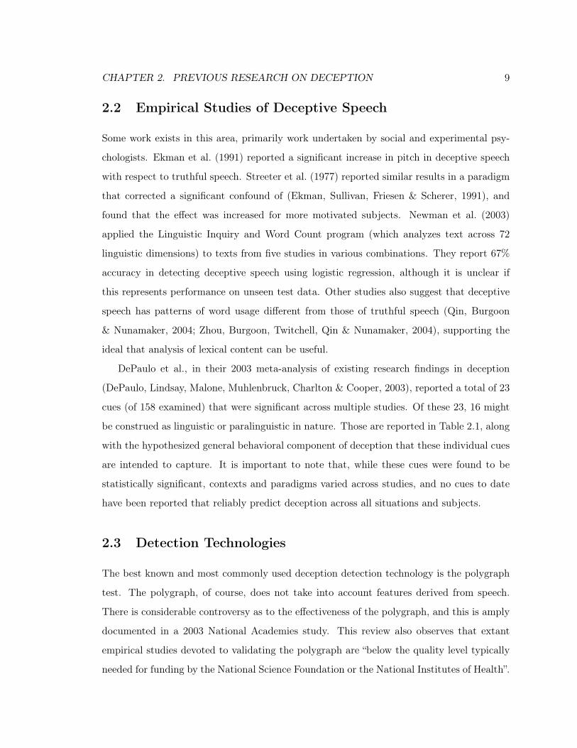
2.2 Empirical Studies of Deceptive Speech
Some work exists in this area, primarily work undertaken by social and experimental psy-
chologists. Ekman et al. (1991) reported a significant increase in pitch in deceptive speech
with respect to truthful speech. Streeter et al. (1977) reported similar results in a paradigm
that corrected a significant confound of (Ekman, Sullivan, Friesen & Scherer, 1991), and
found that the effect was increased for more motivated subjects. Newman et al. (2003)
applied the Linguistic Inquiry and Word Count program (which analyzes text across 72
linguistic dimensions) to texts from five studies in various combinations. They report 67%
accuracy in detecting deceptive speech using logistic regression, although it is unclear if
this represents performance on unseen test data. Other studies also suggest that deceptive
speech has patterns of word usage different from those of truthful speech (Qin, Burgoon
& Nunamaker, 2004; Zhou, Burgoon, Twitchell, Qin & Nunamaker, 2004), supporting the
ideal that analysis of lexical content can be useful.
DePaulo et al., in their 2003 meta-analysis of existing research findings in deception
(DePaulo, Lindsay, Malone, Muhlenbruck, Charlton & Cooper, 2003), reported a total of 23
cues (of 158 examined) that were significant across multiple studies. Of these 23, 16 might
be construed as linguistic or paralinguistic in nature. Those are reported in Table 2.1, along
with the hypothesized general behavioral component of deception that these individual cues
are intended to capture. It is important to note that, while these cues were found to be
statistically significant, contexts and paradigms varied across studies, and no cues to date
have been reported that reliably predict deception across all situations and subjects.
2.3 Detection Technologies
The best known and most commonly used deception detection technology is the polygraph
test. The polygraph, of course, does not take into account features derived from speech.
There is considerable controversy as to the effectiveness of the polygraph, and this is amply
documented in a 2003 National Academies study. This review also observes that extant
empirical studies devoted to validating the polygraph are “below the quality level typically
needed for funding by the National Science Foundation or the National Institutes of Health”.

CHAPTER 2. PREVIOUS RESEARCH ON DECEPTION 10
Table 2.1: Linguistic and Paralinguistic Cues to Deception (DePaulo et al., 2003)
Hypothesis: Liars less forthcoming? Liars less positive, pleasant? Liars more tense?
Cues:a − Talking time − Cooperative + Vocal tension
− Details + Negative, complaining + F0
Hypothesis Liars less compelling? Fewer ordinary imperfections?
Cues: − Plausibility − Spontaneous corrections
− Logical Structure − Admitted lack of memory
− Discrepant, ambivalent + Peripheral details
− Verbal, vocal involvement − Verbal, vocal immediacy
+ Verbal, vocal uncertainty
+ Word, phrase repetitions
aDirection of correlation is indicated with + or −.
(Board, 2003)
Voice stress analysis procedures attempt to rely upon so-called microtremors in the vocal
folds as indicators of stress and by extension of deception. Commercial systems claim to
distinguish truth from lie — or love from indifference — but independent reports fail to
confirm these claims (Haddad & Ratley, 2002; H. Hollien, 2006). Newman et al. (2003), as
described above, apply automatic linguistic techniques to deception detection. Statement
analysis (see e.g. (Adams, 1996)) is a lexical approach (based on anecdotal and some empir-
ical evidence) that some commercial concerns claim to have automated, but we have been
unable to locate scientific literature that validates these systems. Thus, despite the evidence
of cues cited in Section 2.2 from the research community, and a fair amount of belief among
practitioners, there has been relatively little scientific work on the automatic identification
of deceptive speech from acoustic, prosodic, and lexical cues.

CHAPTER 2. PREVIOUS RESEARCH ON DECEPTION 11
2.4 Previous Work on Individual Differences in Deception
It seems reasonable to expect that individual differences in the expression of emotion and
other affective states would represent a prerequisite to the expectation that such differences
exist in deceptive behavior. The emotion literature does provide support for the idea that
individuals vary with respect to the manner and degree to which they express emotion and
affect (Kring, Smith & Neale, 1994), and this phenomenon seems to apply to speech as
well (Banse & Scherer, 1996). Scherer (1986), for example, found that some experimental
subjects elevate F0 under stress, while others decrease F0 under the same stimulus; he
also reports that some actors increase F0 when expressing anger, while others decrease F0.
Scherer attributes these differing responses to different underlying affective states on the
part of the subject. That is, he contends that two subjects may exhibit differing affective
or emotional reactions to the same stimulus, and that this seems to be a more reasonable
explanation than the supposition that there are enormous differences in the properties of the
physiological systems in question — the vocal apparatus of course being of greatest salience
here (1986). With this general principle in mind, we examine the literature on deception,
first with respect to general behavioral cues and then with respect to speech.
2.4.1 Individual differences and non-verbal cues
Some evidence exists to suggest individual differences in behavioral manifestations of decep-
tion. Bradley and Janisse (1981) describe the intriguing and intuitive finding that extroverts
are more detectable than introverts using electrodermal resistance while questioned using a
Control Question Test (CQT) in a mock crime paradigm.2 This finding was consistent with
their hypothesis: they presumed that introverts, who by definition experience greater social
anxiety under all circumstances, would be less detectable due to the “noise” generated by
generalized discomfort. This noise should manifest as increased reactivity in both the truth-
ful and deceptive conditions. In contrast, extroverts, who experience less background social
2In a CQT, the examiner compares the subject’s reaction to control questions — those to which the
subject is expected to react, such as “Have you ever cheated someone who trusted you?” — to the subject’s
reaction to “relevant” questions, such as “Did you take the money?” (that is, the money involved in the mock
crime).

CHAPTER 2. PREVIOUS RESEARCH ON DECEPTION 12
anxiety, should be more detectable in the deceptive condition since the deception itself adds
an element of arousal absent from truthful responses. And in fact, extroverts were shown to
be significantly more detectable in their study (they found no relationship for the person-
ality variable neuroticism). Gudjonsson (1982a) presented results that conflict somewhat
with those of Bradley and Janisse: he found that, in a Guilty Knowledge Test (GKT) using
cards,3 extroversion correlated negatively with skin reactivity (but not detectability) in male
subjects, while in females neuroticism correlated positively with reactivity (but not with de-
tectability). Some public debate ensued among the authors (Gudjonsson, 1982b; Bradley &
Janisse, 1983), centered largely around the desirability of the questioning strategies (CQT
vs. GKT) in relation to the personality variables of interest. Bradley and Janisse made
a convincing case for their methods, however, and they have the added appeal of a sound
theoretical framework.
Vrij (1993) found that subjects who scored high in Public Self-Consciousness (PSC)
were consistently rated more credible by police detectives. In a subsequent study, Vrij et
al. (1997) report the more specific finding that, given information about personal traits of a
subject, the quantity of the subject’s hand movements may be a cue to deception. In their
experiment, subjects were evaluated by self report using a previously validated questionnaire
for their levels of PSC and Ability to Control (their) Behavior (ACB). Vrij et al. hypothesized
that subjects in a mock theft paradigm who were high in self-consciousness would be more
cognizant of the perception that increased hand movements could reflect nervousness and
thereby cue deception; consequently they predicted that high self-consciousness subjects
would exhibit fewer hand movements in the deceptive condition. They further hypothesized
that subjects who scored high in ability to control their behavior would also exhibit fewer
hand movements in the deceptive condition. Both of these hypotheses were essentially borne
out: subjects high in PSC consistently exhibited decreased hand movements in the deceptive
condition while subjects low in PSC increased hand movements during deception. Ability
to Control Behavior combined with PSC to form an additive effect on hand movements:
subjects who scored high in both traits represented the largest category of subjects who
3Subjects choose one from a set of cards without the knowledge of the experimenter. They are then
shown a series of cards and deny having chosen each of them.

CHAPTER 2. PREVIOUS RESEARCH ON DECEPTION 13
decreased hand movements in deception, and subjects low in both traits represented the
largest category of subjects who increased hand movements in deception.
This last finding of Vrij et al. (1997) encapsulates the general message of the study: that
subjects who were low in both ACB and PSC increased hand movements during deception
while most all others either decreased hand movements during deception or maintained
similar frequency of hand movements in both conditions. Vrij and Graham (1997) pursued
the efficacy of this cue for human lie detectors in a perception study: they engaged a group
of students and a group of police officers in a scenario in which subjects viewed videotapes
of deceivers in a mock crime paradigm (a subset of subjects from the previous study (Vrij
et al., 1997)). In the control condition, subjects were asked to determine when the speakers
were lying and when they were telling the truth; in the experimental condition, subjects
were asked to perform the same task, but told in advance in layman’s terms that individuals
who were low in ACB and PSC increased hand movements when lying and that all others
decreased hand movements. These subjects were thus confronted with two tasks: first,
to assess the salient personality traits of the speakers, and then to assess their veracity,
presumably by using the information provided regarding the relationships among personality,
frequency of hand movements, and deception.4 The results of the experiment showed that
students in the experimental group (those who received the information described) performed
significantly better than the student controls (55% vs. 42%; p.01); there was no significant
difference between the two groups of police officers. This result is partly explained by the fact
that students were significantly more accurate than police officers in assessing the personality
traits of the speakers (which the authors attribute to the fact that the speakers were also
students, and thus potentially more easily assessed by fellow students).5 The results of this
study do seem to suggest, however, that knowledge of the effect of personality on deceptive
4The subset of video taped subjects was chosen so that the information provided to the experimental
group was sufficient to allow them to achieve 100% accuracy on the deception detection task provided they
were accurate in their assessment of the personality traits of the speakers (and of course that they were
capable of recognizing an increase or decrease in hand movements).
5Interestingly, police officers as a whole showed a wider range of accuracy scores than students: two
officers in the control group actually scored in the 80–90% range, while the single best performing student
(a member of the experimental group) scored in the 70–80% range.
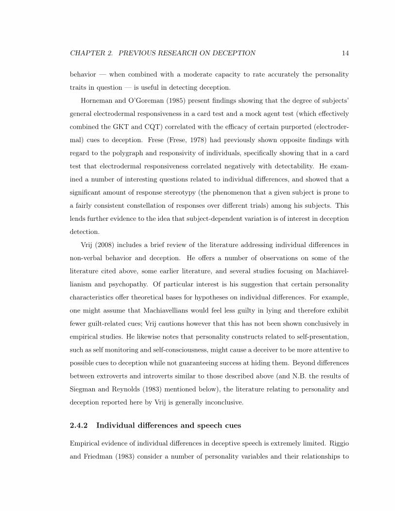
CHAPTER 2. PREVIOUS RESEARCH ON DECEPTION 14
behavior — when combined with a moderate capacity to rate accurately the personality
traits in question — is useful in detecting deception.
Horneman and O’Goreman (1985) present findings showing that the degree of subjects’
general electrodermal responsiveness in a card test and a mock agent test (which effectively
combined the GKT and CQT) correlated with the efficacy of certain purported (electroder-
mal) cues to deception. Frese (Frese, 1978) had previously shown opposite findings with
regard to the polygraph and responsivity of individuals, specifically showing that in a card
test that electrodermal responsiveness correlated negatively with detectability. He exam-
ined a number of interesting questions related to individual differences, and showed that a
significant amount of response stereotypy (the phenomenon that a given subject is prone to
a fairly consistent constellation of responses over different trials) among his subjects. This
lends further evidence to the idea that subject-dependent variation is of interest in deception
detection.
Vrij (2008) includes a brief review of the literature addressing individual differences in
non-verbal behavior and deception. He offers a number of observations on some of the
literature cited above, some earlier literature, and several studies focusing on Machiavel-
lianism and psychopathy. Of particular interest is his suggestion that certain personality
characteristics offer theoretical bases for hypotheses on individual differences. For example,
one might assume that Machiavellians would feel less guilty in lying and therefore exhibit
fewer guilt-related cues; Vrij cautions however that this has not been shown conclusively in
empirical studies. He likewise notes that personality constructs related to self-presentation,
such as self monitoring and self-consciousness, might cause a deceiver to be more attentive to
possible cues to deception while not guaranteeing success at hiding them. Beyond differences
between extroverts and introverts similar to those described above (and N.B. the results of
Siegman and Reynolds (1983) mentioned below), the literature relating to personality and
deception reported here by Vrij is generally inconclusive.
2.4.2 Individual differences and speech cues
Empirical evidence of individual differences in deceptive speech is extremely limited. Riggio
and Friedman (1983) consider a number of personality variables and their relationships to

CHAPTER 2. PREVIOUS RESEARCH ON DECEPTION 15
behavioral cues to deception. Among these are what they call “plausibility”, a subjective
judgement of the credibility of the subject’s statement; and counts of syllables and words
per second. In their study, the differential plausibility scores between the deceptive and
truthful conditions showed no significant relationship to personality. Likewise, the differen-
tial speaking rate measures (which were combined via factor analysis with other variables
into a score for “facial animation”, effectively removing it some distance from the realm of
speech cues), showed no relationship to personality.
Siegman and Reynolds (1983) found that introverts exhibited behavior different from
that of extroverts in deception. In an induced cheating paradigm (ostensibly a test of
subjects extra-sensory perception, in which subjects were encouraged to cheat by a confed-
erate), introverts varied to a greater degree between the truthful and deceptive conditions
on a measure of “verbal fluency” that combined speaking rate, response latency, and pause
duration.
Vrij (2008) likewise offers an analysis of some of the literature on individual differences
in verbal cues to deception, and concludes that, while no overwhelming evidence exists for
such cues, it is too early to conclude that they do not exist. He points, for example, to the
possibility that intelligence might modulate the display of verbal cues in deception since,
presumably, greater intelligence would mitigate the increase in cognitive load associated
with lying.
Although fairly sparse, the literature on individual differences in deception contains
some intriguing findings. As we will detail in Chapter 7, conversations with practitioners
and instructors (for example, see (Reid & Associates, 2000)) of real world interrogation
technique further support the idea that deception is an individualized phenomenon. We will
investigate that idea at some length in Chapter 7.
2.5 Perception Studies
A recent meta-analysis (Aamodt & Custer, 2006) examines the results of 108 studies that
attempted to determine if individual differences exist in the ability to detect deception.
Ability (where chance is 50%) ranged from that of parole officers (40.41%, one study) to

CHAPTER 2. PREVIOUS RESEARCH ON DECEPTION 16
that of secret service agents, teachers, and criminals (one study each) who scored in the 64–
70% range. The bulk of studies (156) used students as judges; they scored on average 54.22%.
Table 2.2 details the results of this analysis by group, and shows that many groups for which
deception detection ability would presumably be career-relevant do not in fact perform
substantially beter than college students. A meta-analysis by Bond and DePaulo (2006)
examining “hundreds of experiments” likewise finds that the mean accuracy of perceivers is
54%. In a subset of studies they found that perceivers who judged exclusively audio data
performed better (53.01% on average) than those who judged exclusively video data (50.5%).
Table 2.2: Are professionals better at detecting deception than students? (Aamodt & Custer,
2006) Used by permission.
Group Studies/Groups N (Subjects) Accuracy%
Teachers 1 20 70.00
Social workers 1 20 66.25
Criminals 1 52 65.40
Secret service agents 1 34 64.12
Psychologists 4 508 61.56
Judges 2 194 59.01
Police Officers 8 511 55.16
Customs officers 3 123 55.30
Federal officers 4 341 54.54
Students 122 8,876 54.20
Detectives 5 341 51.16
Parole officers 1 32 40.42
TOTAL 193 14,379 54.50
Vrij (2008) explicitly considers the frequent mismatch between perceivers’ beliefs about
deception cues and those behaviors that can be shown objectively to be cues to deception.
Vrij’s analysis shows that while subjects are aware of some valid cues, they also hold many

CHAPTER 2. PREVIOUS RESEARCH ON DECEPTION 17
incorrect beliefs, or are simply unaware of relevant cues. For example, while many subjects
correctly consider elevated pitch and the implausibility of speakers’ responses to be cues to
deception, many incorrectly believe that frequent pausing, speech errors, and inconsistency
are valid cues. At the same time, perceivers are unaware that the duration of pauses,
the use of negation, and the length of responses all provide objective cues to deception.6
Vrij additionally offers a number of reasoned theories that seek to explain the origin and
persistence of misconceptions around deception cues.
2.6 Conclusions
The most salient fact about deception, from the perspective of a researcher in the area of
deceptive speech, is that matching human performance would not represent an adequate goal.
There is nevertheless reason to believe speech processing techniques might be successful in
this domain. Although there is little existing work addressing speech, there are a number of
findings to suggest that there is information with discriminative power in the speech signal.
And since virtually none of this literature addresses the application of speech processing
techniques to this task, we consider this to be an area ripe for exploration. Likewise, there
is little literature addressing individual differences in deceptive speech. What work exists,
however, suggests that there is potential for further progress in this area as well.
6The first two of these correlate positively with deception while the last correlates negatively.

Chapter 3. 18
Chapter 3
Columbia-SRI-Colorado (CSC)
Corpus
One of the primary obstacles to research on the automatic detection of deceptive speech has
been the lack of a cleanly-recorded corpus of deceptive and non-deceptive speech for use in
training and testing.1 The CSC Corpus (Hirschberg et al., 2005; Enos et al., 2006) is the first
corpus designed and collected by speech scientists for the purpose of studying the detection
of deceptive speech.2 Prior to undertaking the design and collection of a deception corpus,
the attributes of an ideal dataset were considered. We also considered the possibility that
satisfactory data might already exist. Such data would consist of cleanly recorded speech for
which ground truth (i.e. the veracity of each statement) is known with certainty, recorded
in a real-world scenario in which the stakes — potential for gain or loss, and particularly
the risk of punishment — for the speaker are very high.
1By cleanly-recorded, we mean a corpus of high recording quality with respect to signal-to-noise-ratio,
separation of speakers, and sample rate.
2This human subjects study was authorized by the approval of Columbia University IRB Protocol IRB-
AAAA4209.

CHAPTER 3. COLUMBIA-SRI-COLORADO (CSC) CORPUS 19
3.1 Rationale for collecting
Previous studies, primarily by psychologists, have recorded and studied speech in experi-
mental deceptive scenarios (e.g. (Streeter, Krauss, Geller, Olson & Apple, 1977)). Likewise,
video recordings have been employed in studies of deception or deception detection ability
(see, e.g. (Ekman & Friesen, 1974; Ekman, Sullivan, Friesen & Scherer, 1991)). In both
video and audio scenarios, however, the quality of recordings has not, for the most part,
been sufficiently high for the sort of analysis performed in the present work. This is not
unreasonable, of course, since the aim of these studies has been to examine basic properties
of speech such as intensity and F0 — again, see (Streeter et al., 1977) — rather than to
apply state-of-the-art speech processing methods. Such data do, however, present technical
obstacles when considered in the context of applying more sophisticated speech-processing
techniques.
We also considered using “found” data in which deception occurred, such as television
footage or recordings from actual investigations or trials, since there is certainly no shortage
in the public record of instances of deception on the part of politicians, notorious crimi-
nals, and ordinary people. In most cases, however, we again concluded that the quality of
recording would generally not be sufficient for our purposes, and other obstacles, such as the
presence of multiple concurrent speakers and verification of ground truth, presented likely
difficulties in many cases.3
Given the lack of suitable, existing data, we designed and collected the CSC Corpus.
In what follows it will be clear that we have produced a corpus that is recorded with high
quality, and that ground truth has been adequately established. And as we will describe in
detail below, although in a laboratory setting ethical and practical concerns precluded the
use of a paradigm that involved fear of punishment, subjects were motivated to deceive via
3We of course acknowledge that, to have practical impact, work on deception detection in speech must
be applicable to real-world data. Such practical applications would surely involve the collection of speech
under sub-optimal conditions, such as airports or border checkpoints, and thus would need to be robust to
background noise, crosstalk, and other interference. However, since the work undertaken here is possibly
the first to evaluate the application of state-of-the art speech processing techniques to deception detection,
we determined that optimal recording conditions would be desirable.

CHAPTER 3. COLUMBIA-SRI-COLORADO (CSC) CORPUS 20
the prospect of financial gain and because the scenario was designed to tap into the subjects’
“self-presentational” perspective.
3.2 The corpus
The CSC corpus was designed to elicit within-speaker deceptive and non-deceptive speech.
Speakers were offered the prospect of an additional financial incentive to deceive successfully,
and the instructions were designed to link successful deception to the “self-presentational”
perspective (DePaulo et al., 2003). That is, speakers were told that the ability to succeed
at deception indicated other desirable personal qualities.
3.2.1 Method
The corpus comprises interviews of thirty-two native speakers of Standard American English,
16 male and 16 female, who were recruited from the Columbia University student population
and from the community — primarily via Craig’s List (www.craigslist.com) — in exchange
for payment. (An additional subject’s data had to be discarded because the subject failed
to follow the instructions.) Subjects were recruited for a “communication experiment” and
told (falsely) upon arriving that the study sought to identify individuals who fit a profile
based on the twenty-five “top entrepreneurs of America”. Subjects answered questions and
performed activities in six areas, labeled: music, interactive, survival skills, food and
wine knowledge, NYC geography, and civics. In actuality, the difficulty of tasks was
manipulated so that subjects would find it credible that they had scored too high to fit the
profile in two areas, too low in two, and correctly in two. Four target profiles existed so that
subjects’ lies could be balanced among the six areas. To this end, both an “easy” and “diffi-
cult” set of questions existed for each topic area. In the music section, for example, subjects
who were meant to perform well were asked to sing “Happy Birthday” to the questioner;
subjects who were meant to perform poorly were asked to sing “Casta diva” from Norma.
In the second phase of the study, subjects were shown their scores and told that they
did not fit the target profile, but that the study also sought individuals who did not fit the
profile but who could convince an interviewer that they did. They were told that those

CHAPTER 3. COLUMBIA-SRI-COLORADO (CSC) CORPUS 21
who succeeded at deceiving the interviewer into believing that they had fit the target profile
would qualify for a drawing to receive an additional $100, and would participate in further
aspects of the study. In addition, subjects were told that studies had shown that people
who could convince others that they had particular characteristics often enjoyed many of
the social benefits enjoyed by people who actually had the characteristics in question. This
premise was accepted by our subjects, and the idea that this would provide motivation for
our subjects is fairly intuitive. Ekman et al. (1974), for example, found that experienced,
successful nurses were successful deceivers in a paradigm that related to the domain of
nursing. In the same study, it was shown that for less experienced nurses, the ability to
deceive correlated positively with their supervisors’ evaluations of their skill at working
with patients a year after the study. Ekman (1997) contends that the implication career-
relevance increases the emotional stakes for the deceiver, and we likewise hoped that tying
Figure 3.1: A photograph of the interview setting. (Simulation: no actual subjects are
depicted. Used by permission.)
CHAPTER 3. COLUMBIA-SRI-COLORADO (CSC) CORPUS 22
the subjects’ ability to deceive to their success in other domains might serve to further
motivate them in our study as well. The combination of this claim with the assertion that
the original profile was based on 25 top entrepreneurs has further theoretical grounding in
the construct known in social psychology as “self-presentation” (see (DePaulo et al., 2003)).
Taken as a whole, the paradigm was designed to motivate subjects to lie via both financial
and social incentives.
After taking the initial test and receiving their scores, the subjects (all subjects elected
to continue to the interview portion of the experiment) joined the interviewer in a double-
walled sound booth (see Section 3.2.3 for details of recording conditions) and attempted
to convince him that their scores in each of the six categories matched the target profile.
Because of the design of the pretest described above, each subject was motivated to tell
the truth in two task areas and to deceive the interviewer in four others. The interviewer’s
task was to determine how he thought the subjects had actually performed, and he was
allowed to ask them any questions other than those that were actually part of the tasks
they had performed. The author served as the interviewer for all subjects, and prepared
for the task via conversations with professional practitioners, a review of the literature, and
by taking part in two courses in interviewing and interrogation provided by the John Reid
and Associates (Reid & Associates, 2000) directed at law enforcement and other security
professionals; he additionally employed skills deriving from a previous career as a trained
actor.
Two kinds of lies are implicit in this context. The global lie is the interviewee’s overall
intention to deceive with respect to each score, and by extension, with respect to the most
salient topic of each section of the interview, since the interviewer addressed the individual
topics in discrete sections. The local lie represents statements in support of the reported
score; these statements will be either true or false. The distinction between these types
of lie is subtle but important, since subjects do not always lie at the local level to convey
a global lie. For example, an interviewee may truthfully claim that she has lived in New
York City her whole life to support her false claim that she scored well on her knowledge
of NYC geography. Subjects indicated whether each statement they made was entirely
true or contained some element of deception by pressing one of two pedals hidden beneath

CHAPTER 3. COLUMBIA-SRI-COLORADO (CSC) CORPUS 23
Table 3.1: Subject statistics with interview length in minutes and seconds.
Subject Gender Duration Subject Gender Duration Subject Gender Duration
S-01 M 17:01 S-12 M 12:32 S-23 F 40:00
S-02 F 18:48 S-13 M 16:15 S-24 M 35:53
S-03 M 15:53 S-14 M 20:51 S-25 F 41:56
S-04 M 20:23 S-15 F 23:46 S-26 F 37:38
S-05 M 20:46 S-16 F 33:01 S-27 M 41:00
S-06 F 17:13 S-17 M 38:02 S-28 M 34:06
S-07 F 26:39 S-18 M 26:53 S-29 M 35:04
S-08 F 25:44 S-19 M 21:42 S-30 F 39:41
S-09 M 24:14 S-20 F 32:28 S-31 F 41:09
S-10 F 18:56 S-21 M 28:47 S-32 F 32:48
S-11 F 20:37 S-22 F 54:00
the table (one for TRUTH , the other for LIE). The pedals were connected via serial
ports to a desktop computer located outside of the recording booth, and a Java program
recorded the time and pedal associated with each pedal press. These time stamps and labels
— representing the local lie category — were synchronized with the speech signal in post-
processing. Ground truth was known a priori for the global lie category, since the subjects’
scores on each section were known. The interviews (see Table 3.1) lasted between 25 and 50
minutes, and comprised approximately 15.2 hours of dialogue; they yielded approximately
7 hours of subject speech.
Following the widely employed interrogation strategy promoted by John Reid and Asso-
ciates (2000), a majority of the interviews comprise two parts: an interview and an interroga-
tion. In the interview section, the interviewer attempted to be conversational and generally
non-confrontational, gathering information about the subjects’ claimed performance and
background information justifying those claims. In the interrogation section, the interviewer
was more direct and confrontational, making direct accusations that the subject was lying
or in other ways challenging the subject, for example “Is there any reason that you might

CHAPTER 3. COLUMBIA-SRI-COLORADO (CSC) CORPUS 24
Example 3.3.1: Emotional stakes around lying, subject speech marked (S).
(I) How do you feel about being interviewed to determine whether or not you fit the profile?
(S) I feel very comfortable about it. [LIE]
(I) Why do you think someone would lie about fitting the profile?
(S) Why is s- - why do I think someone would lie about fitting the profile? Because they
wanted to get the money for the experiment. [TRUTH]
(I) Uh, so I’m not saying that you have, but when the experiment was explained to you,
did you consider that you might lie about fitting the profile?
(S) No. [LIE]
(I) Not at all?
(S) No. [LIE]
(I) Tell me why you wouldn’t lie about fitting the profile.
(S) Because I fit- [0.6 second pause] a- th- - I fit the profile. [LIE]
(I) What do you think should happen to someone who lies, in general?
(S) [4 second pause] I think it depends on the situation they’re lying in. [TRUTH]
(I) What about a situation exactly like this one?
(S) Oh. [2.3 second pause] What I think should happen to them? Um, I think that they
should be cast out of the study. [LIE]
not be telling the truth about that particular section?”.
Additionally, we refined our approach to ensuring subjects’ emotional investment in the
paradigm, and to this end an approach was developed that is illustrated by Example 3.3.1.
In this and in analogous exchanges with other subjects, the interviewer’s aim is to increase
the emotional stakes around the topic of lying, and he does this by attempting to draw the
subjects’ attention to the social and other implications of lying, and of being caught in a lie.

CHAPTER 3. COLUMBIA-SRI-COLORADO (CSC) CORPUS 25
3.2.2 Example dialogs
We offer two further examples of excerpted dialog, with the aim of giving the reader an
understanding of the flavor of the interview exchanges and an understanding of some of the
challenges inherent in the deception detection domain.
Example 3.3.2 on page 26 illustrates a deceptive exchange from the Music section of one
subject’s interview. In this exchange, the interviewer asks the subject her score on the Music
section, and she claims that it was “excellent”, while in reality her score was poor. Although
we will not attempt here to convey the prosodic and acoustic aspects of this excerpt, there
are a number of interesting observations to be made based solely on the transcription. First,
the degree of detail in the subject’s initial responses to the question is of note. Although she
is lying, she develops a fairly elaborate story regarding her grandmother’s musical career,
and an heirloom violin of which she (the subject) was the recipient. This degree of detail
lends itself to two opposing interpretations with respect to deception detection lore. On
one hand, the degree of detail might be interpreted as excessive — an attempt to “oversell”
a story. In this regard, one might make note of the seemingly superfluous mention of the
subject’s lack of athletic prowess (a reference to her reported score in the previous interview
section), which is unsolicited in this context, but might be interpreted as an attempt to
drive home the point being made. On the other hand, the degree of detail might simply
derive from the fact that the speaker is relating actual events and memories, which would
necessarily be rich in detail. (We attempt to capture these lexical attributes, incidentally, via
features that measure the length in words and relative length of utterances, and in a feature
that aims to capture the lexical complexity of segments.) As the interview continues, and
particularly as the interviewer asks more specific questions, the specificity of the responses
seems to degrade, and the subject seems to hedge the previous claims. The number of filled
pauses increases, the subject begins to repeat the questions, and a long silent pause occurs
in the last response of the example. Some would claim that all of these phenomena point
to deception. However, as we report in (Benus, Enos, Hirschberg & Shriberg, 2006), in the
CSC Corpus, filled pauses actually correlate with truthful speech.
Example 3.3.3 on page 27 likewise highlights some of the ambiguities inherent in this
domain. In this example, the subject truthfully reports that her score in the Music section

CHAPTER 3. COLUMBIA-SRI-COLORADO (CSC) CORPUS 26
Example 3.3.2: Deceptive exchange in the Music section.
(I) We’ll move on to the next section, which we’re calling the musical section. How did
you do on that section?
(S) I did excellent on that one. Sort of k- k- corresponds with not being a good athlete.
Had to do something right. [LIE]
(I) And so why do you think you did so well on that section?
(S) Um, well, my grandmother was a concert violinist, and she left me her violin. And so
I started playing at a really early age, and so I developed an ear and, you know, it was
just somewhat of an innate thing. [LIE]
(I) Where did your grandmother play?
(S) My grandmother - well, um, okay - she was a concert violinist, but she wasn’t huge.
But she played for the Cape Cod Symphony. [LIE]
(I) And, uh, what kind of violin did she leave you?
(S) It was a really old violin. They weren’t exactly sure who the maker was, but they
thought it was from Germany. [LIE]
(I) And how long have you been playing the violin?
(S) Since I was four. Basically since I could hold the violin. [LIE]
(I) Do you play in the orchestra here?
(S) I don’t - I actually stopped. Um, I I guess I got a little burned out. I just play for
myself mostly now. [LIE]
(I) Who’s your favorite composer for the violin?
(S) Um, my favorite composer. Um, Haydn. [LIE]
(I) What’s the hardest piece you’ve ever played?
(S) Hardest piece, um, [0.8 second silence] that would have to be the Minuet in G Major.
[LIE]
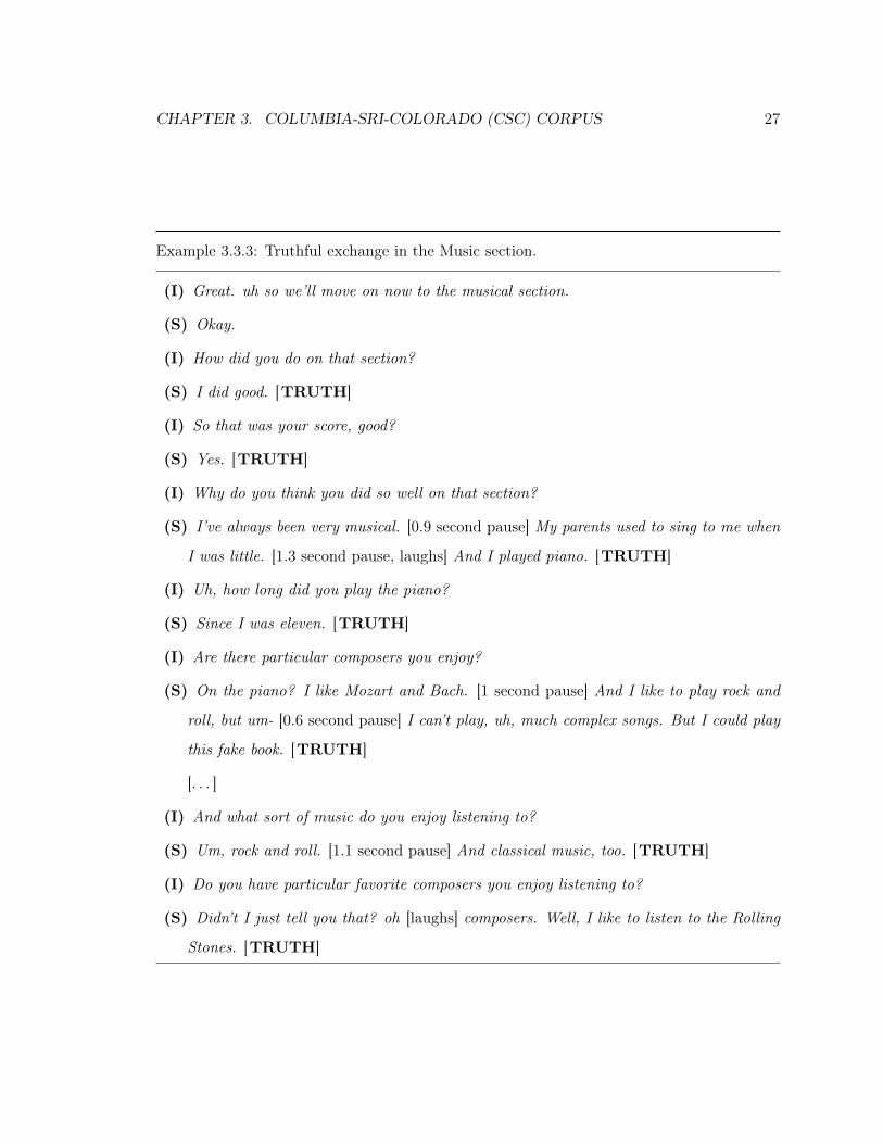
CHAPTER 3. COLUMBIA-SRI-COLORADO (CSC) CORPUS 27
Example 3.3.3: Truthful exchange in the Music section.
(I) Great. uh so we’ll move on now to the musical section.
(S) Okay.
(I) How did you do on that section?
(S) I did good. [TRUTH]
(I) So that was your score, good?
(S) Yes. [TRUTH]
(I) Why do you think you did so well on that section?
(S) I’ve always been very musical. [0.9 second pause] My parents used to sing to me when
I was little. [1.3 second pause, laughs] And I played piano. [TRUTH]
(I) Uh, how long did you play the piano?
(S) Since I was eleven. [TRUTH]
(I) Are there particular composers you enjoy?
(S) On the piano? I like Mozart and Bach. [1 second pause] And I like to play rock and
roll, but um- [0.6 second pause] I can’t play, uh, much complex songs. But I could play
this fake book. [TRUTH]
[. . . ]
(I) And what sort of music do you enjoy listening to?
(S) Um, rock and roll. [1.1 second pause] And classical music, too. [TRUTH]
(I) Do you have particular favorite composers you enjoy listening to?
(S) Didn’t I just tell you that? oh [laughs] composers. Well, I like to listen to the Rolling
Stones. [TRUTH]
CHAPTER 3. COLUMBIA-SRI-COLORADO (CSC) CORPUS 28
was “good”. There are, however, many aspects of the exchange that might engender doubt
about her responses on the part of a listener. Most notably, the subject’s utterances are
peppered with long silent pauses — one as long as 1.3 seconds. Likewise, there are many
filled pauses, which many listeners (including our group of perception subjects; see Chapter
10) associate with deception. Further, the subject laughs at seemingly inappropriate times,
believed by some to be a signal of nervousness and consequently of deception. Finally,
the subject reacts somewhat defensively in the final turn, asserting that she had already
answered the question. Again, an interpretation of this “cue” as indicative of deception
would be in error, as all of the utterances in this example are labeled TRUTH.
3.2.3 Recording and labeling
Interviews were conducted in a double-walled sound booth and recorded to digital audio tape
on two channels using Crown CM311A Differoid headworn close-talking microphones, then
downsampled to 16kHz before processing. Interviews were orthographically transcribed by
hand using the NIST EARS transcription guidelines (NIST, 2004); labels for local lies were
obtained automatically from the pedal-press data and hand-corrected for alignment, and la-
bels for global lies were annotated during transcription based on the subjects’ known scores
versus their reported scores. The orthographic transcription was force-aligned using the
SRI telephone speech recognizer adapted for full-bandwidth recordings (Stolcke, Anguera,
Boakye, Cetin, Grezl, Janin, Mandal, Peskin, Wooters & Zheng, 2005). There are several
segmentations associated with the corpus: the implicit segmentation of the pedal presses,
“breath groups”, derived semi-automatically; sentence-like units (EARS SLASH-UNITS or
SUs (NIST, 2004)), which were hand labeled; and the units corresponding to each topic of
the interview.
3.3 Feature extraction
The CSC dataset currently includes three general classes of features, comprising: acous-
tic/prosodic, lexical, and subject dependent features (Hirschberg et al., 2005). These fea-
tures are enumerated individually and described in detail in Appendix C.

CHAPTER 3. COLUMBIA-SRI-COLORADO (CSC) CORPUS 29
3.3.1 Acoustic and prosodic features
Approximately two-hundred acoustic and prosodic features were extracted using tools
available from automatic speech recognition, including durational, pausing, intonational, and
loudness features.4 Features were extracted using multiple time scales, ranging from a few
milliseconds to an entire utterance. Features are automatically normalized using a variety
of schemes exploiting both long-term speaker-specific habits and local (segmental) context.
Pitch and energy were estimated using the ESPS/Waves pitch tracker get_f0 function; dura-
tional features were obtained using the forced alignment of the hand transcription described
in Section 3.2. Three kinds of pitch features were computed from the voiced regions of each
segment, and were then used in one of three forms: raw; median-filtered; or stylized, by fit-
ting linear splines to the median-filtered pitch. A large set of second-order features were then
computed, including maximum pitch, mean pitch, minimum pitch, range of pitch number of
frames that are rising/falling/doubled/halved/voiced, length of the first/last slope, number
of changes from fall to rise, and value of first/last/average slope. Features were normal-
ized by five different approaches: raw (no normalization), NNORM (divide by the mean),
DNORM (subtract the mean), PNORM (The cumulative distribution function value for
the feature), and ZNORM (subtract the mean and divide by the standard deviation). Two
basic energy features were computed: the raw energy in the segment, and the raw energy of
only the voiced regions. The latter was used in one of three forms: raw, median-filtered, or
stylized as with pitch. Again, several second-order features were computed, including the
maximum, minimum, mean and others. Finally, several durational features were computed.
Maximum and average phone duration in the segment were first computed, then used either
as raw values, normalized using speaker specific durations, or normalized using durations
computed from the whole corpus. Both NNORM and DNORM values for these features
were computed. Finally, many prosodic features (e.g. slope of pitch of last syllable of an
utterance; duration of first syllable of an utterance) were automatically extracted. These
features have been shown to be of use in a variety of structural and paralinguistic tagging
tasks by Shriberg et al. (2004); the approach used here is largely as described by those
4These features were engineered and extracted by colleagues at SRI/ICSI, in particular Martín Gracia-
rena.
CHAPTER 3. COLUMBIA-SRI-COLORADO (CSC) CORPUS 30
authors.
3.3.2 Lexical features
A fair amount of literature suggests that word usage provides important cues to deception
(Newman, Pennebaker, Berry & Richards, 2003; Qin, Burgoon & Nunamaker, 2004; Zhou,
Burgoon, Twitchell, Qin & Nunamaker, 2004); this in turn motivated our exploration of
lexical features. Approximately fifty such features were extracted automatically from the
hand-transcribed text using a variety of methods. The hypotheses motivating the choice of
particular lexical features were based on a number of sources. DePaulo et al. (2003) describe
a number of significant lexical cues to deception, and we have attempted to operationalize
and implement them here. John Reid and Associates, in their courses on interviewing and
interrogation (Reid & Associates, 2000)), as well as the statement analysis literature (Adams,
1996) propose a number of linguistic features that are based on anecdotal and some empirical
evidence. A number of such features are included in the dataset, including simple part-of-
speech and word features (such as the presence of different types of pronouns), contractions,
verb tense, and particular phrases, such as direct denials (e.g. “I did not”). We also capture
cue phrases, (e.g. well, actually, basically); such phrases and particles can be used to mark
discourse structure (Litman & Hirschberg, 1990), and are claimed to be cues to deceptive
speech (Reid & Associates, 2000; Adams, 1996).
A number of details with respect to the lexical features are worth noting. Those features
that entail part-of-speech tags were derived using the QTag (Mason, 2005) probabilistic
tagger. This tagger is widely used, and is reported to perform with approximately 97%
accuracy on text corpora (Madsen, Larsen & Hansen, 2004); we were unable to find reference
to its accuracy on spontaneous speech. Features such as hasI (the presence of the pronoun
I ) that did not entail part-of-speech tags were captured using simple pattern matching.
Features that entail punctuation (e.g. PUNCT, the punctuation label) refer to the punctuation
applied to the given segment by the transcriber. Lexical features that include the term slash
in the name refer to the EARS (NIST, 2004) convention of following transcribed punctuation
with the “/” symbol. Thus, slash_TCOUNT captures the number of punctuation labels in the
segment, while dash_slash_TCOUNT captures the number of “-/” symbols in the segment,
CHAPTER 3. COLUMBIA-SRI-COLORADO (CSC) CORPUS 31
effectively signaling sentence fragments. The complexity feature is a simple ratio of the
number of syllables in the segment divided by the number of words in the segment. The
feature hasNaposT signals the “n’t” contraction, a construct thought by practitioners to be
relevant to deception (Reid & Associates, 2000).
We also captured the presence of positive and negative emotion words, as described
in Section 5.1. Other features captured: whether or not the utterance was a question or
a question following an interviewer question (again, based on the punctuation applied by
the transcriber), and the number of words repeated from the interviewer’s previous query
(indicating hedging behavior (Reid & Associates, 2000)). A number of features might be
described as lexical or pseudo-lexical, such as the presence of mispronounced or unintelligible
words, the count of words in a segment, and the ratio of word count to segment length. Again,
all of these were extracted based on the hand transcription. Finally, we include in our lexical
features a label that indicates the topic of the interview section (music, interactive, etc.).
Additional details regarding these and other features may be found in Appendix C.
We employed a number of paralinguistic features, which include counts of laughter,
instances of speaker noise, audible breaths, and self-repairs, all of which were extracted
using the relevant tags in the hand transcription (Vrij & Winkel, 1991; Ekman, 2001; Reid
& Associates, 2000).
There are a number of limitations to the lexical features employed. First, some, such
as hasPastParticipleVerb or verbWithIng may capture morphological phenomena rather
than syntactic phenomena so that the former would not distinguish between the past par-
ticiple and the passive, while the latter would not distinguish between the progressive and
the gerund used as a noun. The feature hasNaposT conflates the contraction and the nega-
tive. Additionally, though we included hasNaposT and other individual features that capture
negative constructs (hasNot, hasNo), we did not capture the simple presence of negation.
Likewise, hasI and hasWe are included, but we do not include a single feature that captures
the presence of the first person. Finally, we acknowledge that the inclusion of the topic
feature is corpus-specific, but it is reasonable to believe that an analogous feature could be
computed in other domains where multiple topics were addressed in an interview.

CHAPTER 3. COLUMBIA-SRI-COLORADO (CSC) CORPUS 32
3.3.3 Subject-dependent features
Finally, a class of five subject dependent features were motivated by conversations with
practitioners at the 2004 Center For Advanced Study of Language (CASL) Workshop on
Detecting Deception in Language and Cultural Context and in other venues, and by the
work of O’Sullivan et al. (O’Sullivan & Ekman, 2004). In various ways, these resources
suggest that, since there seems to be no “Pinocchio effect”, that is, a universal deception
response common to all subjects in all contexts (Vrij, 2008), progress in deception detection
may depend to some degree on the ability of approaches to capture baseline behavior of
individuals and to examine deviations from these baselines as potential cues to deception.
To this end, the current feature set includes features that capture phenomena such as: the
ratio of the number of filled pauses in lies to the number of filled pauses in truths; the ratio
of cue phrases in lies to the number of cue phrases in truths; the ratio of segments with
these attributes (cue phrases or filled pauses) to total speaker segments, and gender. These
features were computed as follows: for a given measure (such as ratio of filled pauses in lies
to filled pauses in truths), the ratio was computed for each subject. All subject data were
then pooled and subjects were assigned to quartiles with respect to the pooled data and
their given score. The feature value assigned to the subject was thus an integer from (0...3),
such that a subject scoring in the lowest quartile was assigned the value 0 for all segments.
These features are of course computed using knowledge of the class labels, and all subject
data were used in this process. The use of training data to compute these ratios is mitigated
by two factors: first, for the majority of the classification results we will report, we employ
10 × 10-fold cross-validation, for a total of 100 random trials and one-hundred random
90%/10% data splits. The Law of Large Numbers suggests that the average value for the
feature as computed over these one-hundred 90% samples should tend strongly toward the
true value. Second, any differences that might still exist between the true value and that
achieved by repeated random sampling would likely be mitigated by assignment to quartiles,
which effectively cancels the effect of any variance of ±12.5% (with respect to the subject’s
percentile score) from the center of each quartile.
Two additional observations with respect to the subject dependent features are relevant.
First, we chose to employ quartiles rather than the raw ratios because those ratios, which

CHAPTER 3. COLUMBIA-SRI-COLORADO (CSC) CORPUS 33
were generally unique for each subject, would serve to identify individual subjects, possibly
providing an unfair advantage to the learning algorithms by allowing them to take advantage
of differing class distributions across subjects. Second, we acknowledge that these features,
since they require labeled data from each subject, would preclude the application of the
learned model to a previously unseen subject for which no training data is available, unless
it were possible to predict that subject’s membership in a quartile using some other means.
3.4 Discussion
The paradigm described here is imperfect in several ways, and we offer several suggestions
for future work in Part V. However, it also has many useful attributes. In our scenario
subjects lie about events that actually occur, in contrast with, for example an “inflated
resume” scenario, where subjects simply misrepresent facts that are not necessarily related
to actual events. Likewise, subjects accepted the motivation presented to them with regard
to our desire to find individuals fitting the purported profile; in fact none of them challenged
this premise, and none claimed to have disbelieved it during subsequent debriefing. Further,
given subjects’ reports in the debriefing and our observations in the interview process, we
believe that we engendered a reasonable degree of emotional investment on their parts via
our appeals to self-presentational concerns and financial gain. Here, too, we found that the
subjects did not challenge the premise presented with regard to the association of deception
skills with desirable social qualities.
We would be remiss if we did not address here the issue of the deception of our subjects
inherent to this paradigm. These deceptions were primarily three: that we sought subjects
for a communication experiment that fit a particular profile; that the subjects had not fit
the profile (and the concomitant manipulation of the test); and the unverified claim that
people who can convince others that they have certain qualities often enjoy the benefits of
those qualities. In our review of the literature, we found that successful deception paradigms
frequently entail deception — this is perhaps most true of the “induced cheating paradigm”.5
5We coin this term for paradigms in which subjects are convinced by a confederate to cheat — for
example, at what they believed to be a test of extra-sensory perception — and then confronted afterwards
by the experimenter. See, for example, (Siegman & Reynolds, 1983).

CHAPTER 3. COLUMBIA-SRI-COLORADO (CSC) CORPUS 34
We concluded that deceptions employed here were necessary to capturing the sort of data
we required, particularly given that we felt it imperative to create a scenario in which the
speakers lied about actual salient events rather than simply pretending, or pretending to lie.
We not that, upon debriefing, our subjects were unanimously undisturbed by the deceptions
entailed. Indeed, many expressed fascination with the project and its aims.
In all, the collection of this corpus represents a milestone in the study of deceptive speech,
particularly from the standpoint of speech science. To our knowledge, this corpus is the first
audio corpus of deceptive and non-deceptive speech recorded under conditions that permit
sophisticated acoustic analyses, for example to extract reliable pitch, intensity, and prosodic
characteristics over the entire corpus. It is also unusual in its differentiation between lies
on the local dimension — corresponding to ground-truth information indicated by subjects
on a per-turn basis — and on the global dimension — corresponding to the congruence
of subjects’ claimed scores for each section with their “actual” (assigned) scores on the pre-
test. Finally, we plan to release this corpus for general research use, and it will provide one
standard dataset against which future work can be tested; other researchers have already
expressed interest in this regard.

PART II. 35
Part II
General Analysis and Classification
Chapter 4. 36
Chapter 4
Statistical Analysis
In this chapter, we report an exploratory statistical analysis of the binary and numeric
features of our base feature set, capturing lexical, paralinguistic, discourse, acoustic and
prosodic aspects of speech. We performed this analysis with respect to the local lie labeling
of the data using SUs as our unit of analysis.
4.1 Statistical Methods
There are three broad classes of features represented in the CSC feature set: binary lexi-
cal, paralinguistic and discourse features; lexical, paralinguistic and discourse features that
are expressed numerically (generally as counts of occurrences per segment); and numerical
acoustic and prosodic features. We describe below how each of these classes of feature is
treated.
We analyzed lexical features that are represented in the corpus as binary variables (such
as hasContraction) in terms of tables of counts, and applied the Chi-Square test for
homogeneity to examine whether the distributions of these features differed significantly
between the local lie and local truth conditions. Although not always the case in speaker
dependent analyses (which we take up in Chapter 8), the aggregate data analyzed in the
present chapter met the standard requirement that each cell in the given 2 × 2 contingency
table (representing the four possible conditions: local lie expressing the feature; local
lie omitting the feature; and likewise for local truth ) have an expected value of at least 5.

CHAPTER 4. STATISTICAL ANALYSIS 37
We thus report results here (in some cases, simply that no significant effect was detected)
for all binary features.
Those lexical paralinguistic, and discourse features that are expressed numerically, such
as counts of repeated words or filled pauses, were examined along with the numerical acoustic
and prosodic features. Because inspection shows that a substantial number of features in
these three classes are not normally distributed in the CDC data set, we chose to use to use
two non-parametric tests: the Mann-Whitney U test and the Kolmogorov-Smirnov
test . Both of these tests are used in cases where Student’s T test might be desirable
because of experimental design but would not be valid because of the distribution of the
data in question.
The Mann-Whitney U test employs rank ordering of the data to test whether two
samples “represent two populations with different median values” (Sheskin, 2007), that is,
the null hypothesis is that both samples are drawn from the populations with equal medians.
In the present case, H0 is the proposition that the sample containing TRUTH segments
has the same median as the sample containing LIE segments. When we refer to “significant”
results in what follows, we make the assertion that the preceding H0 is rejected at the speci-
fied significance level(s), and the p-values in question represent the two-tailed p-value, since
no a priori hypothesis is made with respect to the direction of the difference. The present
data generally meet the standard assumptions of the Mann-Whitney U test (Sheskin,
2007) with respect to random selection and the homogeneity of variance of the underlying
distributions. As with any statistical analysis of speech features on the suprasegmental level,
caution must be exercised with regard to the assumption of statistical independence, since
the literature does not provide conclusive evidence either to support or to contradict this
assumption (Julia Hirschberg, personal communication, July 17, 2008); we offer this caveat
and proceed in applying these tests, as is regularly practiced in the literature.
The Kolmogorov-Smirnov test is also a test of central tendency, but in addition
is sensitive to differences in the shape of the distribution. The Kolmogorov-Smirnov
test constructs the cumulative probability distribution for each sample, and tests for a sig-
nificant difference at any point along the two distributions.1 Such a difference suggests with
1Specifically, the two cumulative probability distributions are constructed, and the magnitude of the

CHAPTER 4. STATISTICAL ANALYSIS 38
high likelihood that the samples are taken from different populations. The null hypothesis
in this case is thus that the “distribution of data in the population that Sample 1 is derived
from is consistent” with that of the population of Sample 2 (Sheskin, 2007). In the case of
the current data, rejection of the null hypothesis for a given speaker and feature suggests
that the distribution for the LIE condition differs in shape and/or location from that of
the TRUTH condition for that subject. As with the Mann-Whitney U test , two-tailed
p-values are employed here.
With regard to the combination of the two tests, it should be further noted that, in cases
where the Kolmogorov-Smirnov test shows significant results, the assumption of homo-
geneity of variance is less strongly supported for the Mann-Whitney U test . However,
because in those cases the Kolmogorov-Smirnov test itself (a less sensitive test than
the Mann-Whitney U test) indicates a significant difference in the distributions of two
conditions, we of course maintain that these results are of interest.
4.2 Binary Lexical Features
Our binary feature set comprises 25 lexical, discourse, and pause features (for descriptions,
see Section 3.3.2; for definitions see Appendix C) that capture a number of potential cues
that have either been proposed by practitioners or examined in the literature. They include
flags for the presence of various pronouns, contractions, disfluencies, discourse phenomena
(e.g. questions), verb tenses, negations and positive and negative emotion words.
Table 4.1 reports results of the Chi-squared analysis of binary features; significance values
are indicated for features significant at the 0.05 or better level; an italicized p-value indicates
a negative correlation with deception.
Examination of Table 4.1 reveals that only eight of the 25 features show significant effects
for deception in the aggregate data. The present chapter represents the first reporting on
the statistical analysis of these features in the CSC Corpus, except as noted below, and for
features where such analyses have previously been conducted, they are consistent with those
earlier results.
greatest vertical distance at any point along the distributions is tested for significance.

CHAPTER 4. STATISTICAL ANALYSIS 39
Table 4.1: χ2 significance of binary lexical features: italics ⇒ decreased incidence of the
tested phenomenon in the LIE condition.
Feature p-value Feature p-value
hasFilledPause 0.000 hasPastTenseVerb ns
question 0.001 hasPastParticipleVerb ns
questionFollowQuestion 0.001 verbBaseOrWithS ns
thirdPersonPronouns 0.002 verbWithIng ns
possessivePronouns ns hasNaposT 0.041
hasI ns hasNot 0.020
hasWe ns hasYes ns
specificDenial ns hasNo ns
hasCuePhrase 0.031 noYesOrNo ns
hasSelfRepair ns isJustYes ns
hasContraction ns isJustNo ns
hasPositiveEmotionWord 0.015 hasAbsolutelyReally ns
hasNegativeEmotionWord ns
As in our earlier work in Benus et al. (2006), we found here that filled pauses occur less
frequently with deception. The remainder of the literature is ambiguous with respect to the
utility of filled pauses as a cue (DePaulo et al., 2003), but Vrij (2008) points out that it is a
commonly held misconception that filled pauses and other speech disturbances are reliable
cues to deception.
We capture question-asking behavior in our subjects, as practitioners (Reid & Asso-
ciates, 2000), the statement analysis literature (Adams, 1996), and DePaulo et al. (2003)
all suggest in various ways that topic-changing or avoidant behavior (termed by DePaulo
“holding back”) is indicative of deception; Reid et al. specifically refer to the situation where
a subject responds to a question with a question. We found that these question-asking
features were significant, but that they actually occurred with truthful speech. An alterna-

CHAPTER 4. STATISTICAL ANALYSIS 40
tive interpretation to the avoidance theory is the straightforward possibility that truthful
subjects ask questions in order to promote communication.
In the CSC Corpus, the use of third person pronouns increases with deception, and this
is consistent with the findings of DePaulo et al. (2003) and Hancock (2004). Newman et al.
(2003), however, report the opposite.
Our cue phrase feature captures 33 discourse markers and/or hedges, such as actually,
basically, also and ok, and these again were gleaned from conversations with practitioners,
standard interview training (Reid & Associates, 2000), and the statement analysis literature
(Adams, 1996), all of which suggest that deceptive speech should contain more such cues;
our finding is consistent with these claims, but not to the degree of significance reported for
the other features we have examined thus far.
We find that the use of positive emotion words increases with deception, and this is
consistent with the findings of Burgoon et al. (2003), who found a greater incidence of both
negative and positive emotion words in deceptive speech. Newman et al. (2003) report a
higher incidence of negative emotion words in deception.
Two binary features that capture the presence of negation, hasNot and hasNaposT, show
increases in the deceptive condition. This is consistent with the findings of Adams et al.
(2006) and DePaulo et al. (2003), who report a positive correlation between deception and
negation; Hancock (2004) finds no effect.
We will offer further observations and interpretation of these results after considering
the analysis of our numerical features.
4.3 Numerical Features
Table 4.2 enumerates the base numerical features of our dataset, all of which were sub-
jected to statistical analysis for the present chapter. By “base” feature, we mean the raw
acoustic/prosodic features described in Appendix C whose names do not reference a normal-
ization scheme, such as “PNORM”. For the purposes of statistical analysis of the aggregate
corpus, these features were normalized within speaker on the interval [−1, 1] using the uni-
form distribution. We subjected each feature to analysis using both the Mann-Whitney U
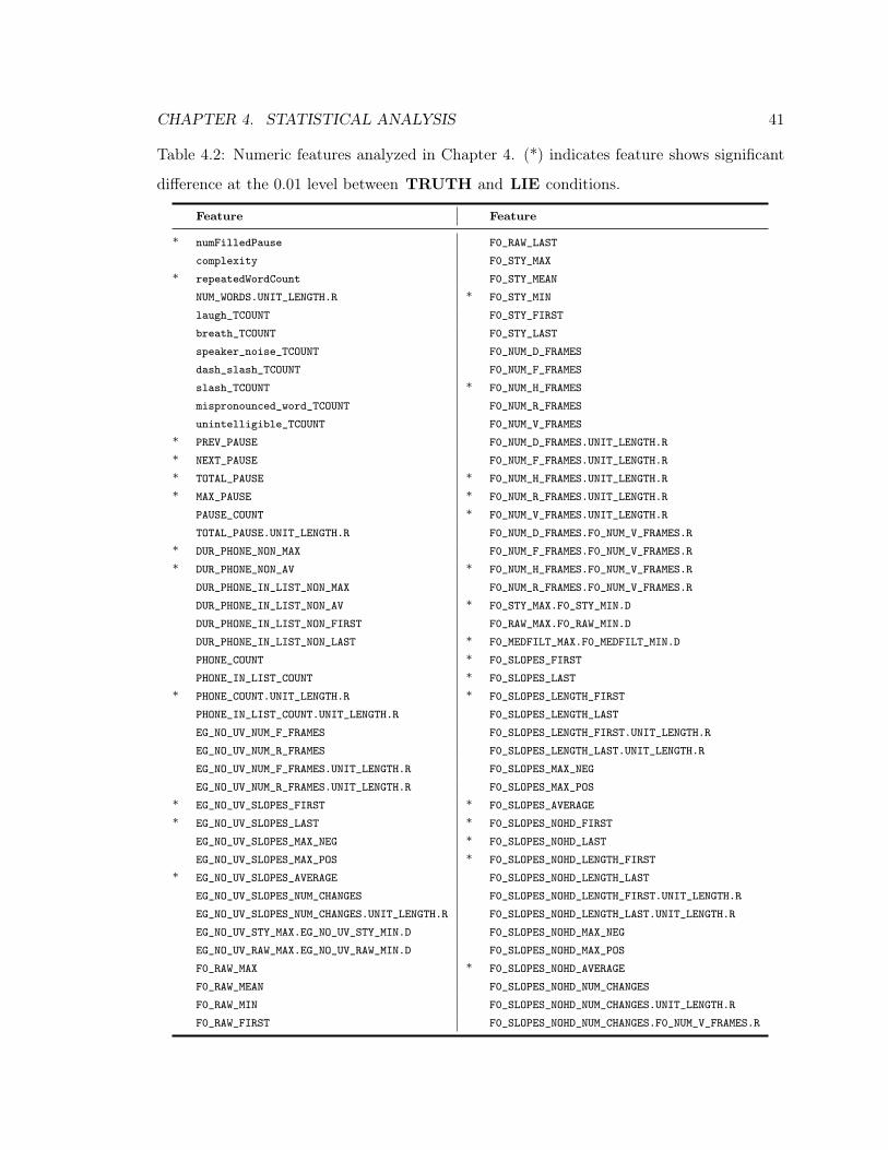
CHAPTER 4. STATISTICAL ANALYSIS 41
Table 4.2: Numeric features analyzed in Chapter 4. (*) indicates feature shows significant
difference at the 0.01 level between TRUTH and LIE conditions.
Feature Feature
* numFilledPause F0_RAW_LAST
complexity F0_STY_MAX
* repeatedWordCount F0_STY_MEAN
NUM_WORDS.UNIT_LENGTH.R * F0_STY_MIN
laugh_TCOUNT F0_STY_FIRST
breath_TCOUNT F0_STY_LAST
speaker_noise_TCOUNT F0_NUM_D_FRAMES
dash_slash_TCOUNT F0_NUM_F_FRAMES
slash_TCOUNT * F0_NUM_H_FRAMES
mispronounced_word_TCOUNT F0_NUM_R_FRAMES
unintelligible_TCOUNT F0_NUM_V_FRAMES
* PREV_PAUSE F0_NUM_D_FRAMES.UNIT_LENGTH.R
* NEXT_PAUSE F0_NUM_F_FRAMES.UNIT_LENGTH.R
* TOTAL_PAUSE * F0_NUM_H_FRAMES.UNIT_LENGTH.R
* MAX_PAUSE * F0_NUM_R_FRAMES.UNIT_LENGTH.R
PAUSE_COUNT * F0_NUM_V_FRAMES.UNIT_LENGTH.R
TOTAL_PAUSE.UNIT_LENGTH.R F0_NUM_D_FRAMES.F0_NUM_V_FRAMES.R
* DUR_PHONE_NON_MAX F0_NUM_F_FRAMES.F0_NUM_V_FRAMES.R
* DUR_PHONE_NON_AV * F0_NUM_H_FRAMES.F0_NUM_V_FRAMES.R
DUR_PHONE_IN_LIST_NON_MAX F0_NUM_R_FRAMES.F0_NUM_V_FRAMES.R
DUR_PHONE_IN_LIST_NON_AV * F0_STY_MAX.F0_STY_MIN.D
DUR_PHONE_IN_LIST_NON_FIRST F0_RAW_MAX.F0_RAW_MIN.D
DUR_PHONE_IN_LIST_NON_LAST * F0_MEDFILT_MAX.F0_MEDFILT_MIN.D
PHONE_COUNT * F0_SLOPES_FIRST
PHONE_IN_LIST_COUNT * F0_SLOPES_LAST
* PHONE_COUNT.UNIT_LENGTH.R * F0_SLOPES_LENGTH_FIRST
PHONE_IN_LIST_COUNT.UNIT_LENGTH.R F0_SLOPES_LENGTH_LAST
EG_NO_UV_NUM_F_FRAMES F0_SLOPES_LENGTH_FIRST.UNIT_LENGTH.R
EG_NO_UV_NUM_R_FRAMES F0_SLOPES_LENGTH_LAST.UNIT_LENGTH.R
EG_NO_UV_NUM_F_FRAMES.UNIT_LENGTH.R F0_SLOPES_MAX_NEG
EG_NO_UV_NUM_R_FRAMES.UNIT_LENGTH.R F0_SLOPES_MAX_POS
* EG_NO_UV_SLOPES_FIRST * F0_SLOPES_AVERAGE
* EG_NO_UV_SLOPES_LAST * F0_SLOPES_NOHD_FIRST
EG_NO_UV_SLOPES_MAX_NEG * F0_SLOPES_NOHD_LAST
EG_NO_UV_SLOPES_MAX_POS * F0_SLOPES_NOHD_LENGTH_FIRST
* EG_NO_UV_SLOPES_AVERAGE F0_SLOPES_NOHD_LENGTH_LAST
EG_NO_UV_SLOPES_NUM_CHANGES F0_SLOPES_NOHD_LENGTH_FIRST.UNIT_LENGTH.R
EG_NO_UV_SLOPES_NUM_CHANGES.UNIT_LENGTH.R F0_SLOPES_NOHD_LENGTH_LAST.UNIT_LENGTH.R
EG_NO_UV_STY_MAX.EG_NO_UV_STY_MIN.D F0_SLOPES_NOHD_MAX_NEG
EG_NO_UV_RAW_MAX.EG_NO_UV_RAW_MIN.D F0_SLOPES_NOHD_MAX_POS
F0_RAW_MAX * F0_SLOPES_NOHD_AVERAGE
F0_RAW_MEAN F0_SLOPES_NOHD_NUM_CHANGES
F0_RAW_MIN F0_SLOPES_NOHD_NUM_CHANGES.UNIT_LENGTH.R
F0_RAW_FIRST F0_SLOPES_NOHD_NUM_CHANGES.F0_NUM_V_FRAMES.R

CHAPTER 4. STATISTICAL ANALYSIS 42
test and the Kolmogorov-Smirnov test , and report those results below. Features that
demonstrated a significant effect for deception are marked with an asterisk in Table 4.2.
4.3.1 Results and discussion
Table 4.3 details the results of our analyses. Of the 88 features examined, 28 showed signif-
icance at the 0.01 level for at least one of the two tests applied;2 14 showed significance for
both tests. The distributions of features for the two classes can be examined in the box plots
of Figures 4.1 through 4.3 on pages 47–49. That many of these features are not normally
distributed is evident from the plots (the normalization method preserves the general shape
of the distributions), and this further points out the utility of the Kolmogorov-Smirnov
test in detecting differences in behavior, since clearly some differences are more due to the
shape of the distributions than to great differences between means or the central tendency.
In fact, in most cases where only one test is significant, this test is the Kolmogorov-
Smirnov test . Inspection of the box plots reveals that in most of these cases, the visible
differences lie on the edges of the distributions rather than in the centers. In the cases where
only the Mann-Whitney U test is significant, we attribute this to the combination of
small differences in the central tendency and the greater sensitivity of the Mann-Whitney
U test to such differences.
In this section we will make observations about those features that showed significance,
and indicate where the behavior observed is (or is not) consistent with the literature. We
will, however, delay a detailed analysis of the features and the behaviors they reflect until
the subject-dependent analysis of Chapter 8, which offers, in the variety of behavior found
across different subjects, a more rich set of behaviors to compare.
Filled pauses again show significance here, in both tests, and the finding is consistent
with our previous observation that such disfluencies happen more often in truthful speech.
The repetition of words occurs more frequently in the TRUTH condition. DePaulo
(2003) found that repetition appears more frequently in the deceptive condition, treating it
2We limit our discussion to features significant at the 0.01 level because of the large sample size (9068
segments) and the sensitivity of the test. The magnitude of the differences captured at this level is evident
in the box plots described below.

CHAPTER 4. STATISTICAL ANALYSIS 43
Table 4.3: Statistical analysis of speaker-normalized numerical features. (*) indicates sig-
nificance in both tests.
Mann-Whitney Kolmogorov-Smirnov
Feature LIE Effect p-value LIE Effect p-value
numFilledPause* less <0.001 less 0.005
repeatedWordCount ns less 0.009
PREV_PAUSE* greater <0.001 greater 0.001
NEXT_PAUSE* greater <0.001 greater 0.001
TOTAL_PAUSE* less 0.003 less 0.003
MAX_PAUSE* less 0.003 less 0.001
DUR_PHONE_NON_MAX* less <0.001 less <0.001
DUR_PHONE_NON_AV* less <0.001 less 0.001
PHONE_COUNT.UNIT_LENGTH.R greater 0.009 ns
EG_NO_UV_SLOPES_FIRST ns greater <0.001
EG_NO_UV_SLOPES_LAST* greater 0.006 greater 0.002
EG_NO_UV_SLOPES_AVERAGE* less <0.001 less <0.001
F0_NUM_H_FRAMES* greater <0.001 greater <0.001
F0_NUM_H_FRAMES.UNIT_LENGTH.R greater <0.001 greater <0.001
F0_NUM_R_FRAMES.UNIT_LENGTH.R ns greater 0.007
F0_NUM_V_FRAMES.UNIT_LENGTH.R greater <0.001 greater <0.001
F0_NUM_H_FRAMES.F0_NUM_V_FRAMES.R greater <0.001 greater <0.001
F0_STY_MIN ns greater 0.003
F0_STY_MAX.F0_STY_MIN.D less 0.006 less 0.005
F0_MEDFILT_MAX.F0_MEDFILT_MIN.D ns less 0.006
F0_SLOPES_FIRST ns less 0.004
F0_SLOPES_LAST* less 0.006 less <0.001
F0_SLOPES_LENGTH_FIRST* less 0.005 less 0.002
F0_SLOPES_AVERAGE ns less 0.001
F0_SLOPES_NOHD_FIRST* less <0.001 less <0.001
F0_SLOPES_NOHD_LAST ns less 0.008
F0_SLOPES_NOHD_LENGTH_FIRST less 0.009 ns
F0_SLOPES_NOHD_AVERAGE* less 0.001 less 0.004

CHAPTER 4. STATISTICAL ANALYSIS 44
as part of their consideration of fluency; Vrij (2008) found repetition to be inconclusive. Here,
we wonder if its correlation with truthful speech might be an aspect of DePaulo’s observation
that in general, truth tellers exhibit more ordinary imperfections than deceivers.
Four silent pause features show significant effects, and seem to capture an interesting
phenomenon. While two features — the total duration of silent pauses in a segment and
the maximum duration of a silent pause for the segment — correlate with TRUTH, two
features capturing the length of the pauses immediately preceding and following a given
segment correlate with LIE. This suggests that, while the truth teller exhibits pausing dur-
ing a segment, the deceiver inhibits such segment-internal pausing. In contrast, pauses of
increased length occur on either side of deceptive segments. In the case of contiguous sub-
ject segments (where the preceding and following SUs were produced by the subject), this
might reflect increased cognitive load entailed by production of the deceptive segment (and
this case of contiguous segments dominates the data, as inspection reveals that most subject
turns contain multiple SUs). The second general case is that the segment is turn-initial or
turn-final. In this case, the two features are dependent on the interviewer’s turn-length, and
though we can speculate with regard to the implications of this (e.g. that the interviewer’s
response to a deceptive subject utterance is longer), we hesitate to make strong claims. Ad-
ditionally, a feature capturing the ratio of the number of voiced frames to the segment length
(F0_NUM_V_FRAMES.UNIT_LENGTH.R) also showed an increase in the LIE condition and may
reflect increased speaking rate or decreased internal pausing in the deceptive condition. The
literature is ambiguous regarding silent pauses and deception; we will take this up in detail
in Chapter 8.
Two durational features (measuring phone duration) are significant here, signaling shorter
duration in deceptive speech. This is inconsistent with the one mention of a similar measure
of which we are aware in the literature: Hall (1986) examined syllabic duration of (one
word) Control Question Test polygraph responses, and found increased duration in decep-
tive answers. Perhaps here it is indicative of more clipped or rushed speech in the deceptive
condition.
Three energy slope features are significant, and again in an interesting constellation:
while values for the first and last slopes of a segment are greater in deception, the average

CHAPTER 4. STATISTICAL ANALYSIS 45
energy slopes of a segment correlate negatively with deception. This suggests (to resort to
language from the singing domain) a stronger “attack” and “release” in deceptive segments,
with, on average, a decline in energy over the course of the segment. This is in a way
consistent with the pausing behavior we observed earlier, in that it represents greater control
once the deceptive segment is initiated than on either side of it, again, possibly an artifact
of the cognitive load associated with deception. The smaller average energy slopes seem to
be consistent with one study (Sayenga, 1983) that found decreased amplitude in deceptive
speech; the literature is otherwise inconclusive around energy or amplitude (see Chapter 8
for further detail).
A number of features measuring pitch halving show positive correlation with deception.3
This seemed curious at first, but there is actually a fairly grounded interpretation to be made
of the relationship of pitch halving to deception. There is evidence that this phenomenon
occurs in the presence of vocal fry or diplophonia (where two pitches are produced by the
speaker at the same time) (Johnson, 2003), and personal experience tells us that both of
these conditions can occur as a consequence of “forced” or overly energetic speech production,
possibly suggesting that the speaker is “overselling” the lie. And there is precedent in the
literature for the use of pitch mistracking in the identification of affective state: Liscombe
(2007), for example, found that mistracks were a helpful cue to the emotion sadness.
With the exception of minimum stylized pitch F0_STY_MIN, which correlates positively
with deception, the large number of significant pitch features — generally capturing range
and slope — features all correlate negatively with deception, painting a picture of speech that
is falling or flat. Pitch has been the speech feature of perhaps most interest in the existing
deception literature (Streeter, Krauss, Geller, Olson & Apple, 1977; Scherer, Feldstein, Bond
& Rosenthal, 1985; Hall, 1986; Ekman, Sullivan, Friesen & Scherer, 1991), and findings have
generally suggested that pitch increases in the deceptive condition. Our finding regarding
F0_STY_MIN seems to be consistent with previous results, but to our knowledge there is no
existing literature that addresses the more complex prosodic features we report here.
3Pitch halving is the misestimation of the pitch on the part of the pitch tracker by a factor of 0.5; pitch
doubling is likewise misestimation by a factor of 2.

CHAPTER 4. STATISTICAL ANALYSIS 46
4.4 Conclusions
We have examined our base set of binary and numeric features, and have shown significant
effects for deception for 36 of the 88 features. Many of these results are consistent with
other findings in the literature, or with our previously reported findings on the CSC Corpus.
We also examined a number of features that have no precedent in the deception literature,
and reported a number of interesting results regarding those features, for example results
relating to voice quality and to the onset and release of speaker segments. We believe
these results demonstrate that our approach — to apply sophisticated speech processing
techniques to deceptive speech — can yield a number of new insights not possible with the
simpler approaches previously taken to the analysis of deceptive speech.
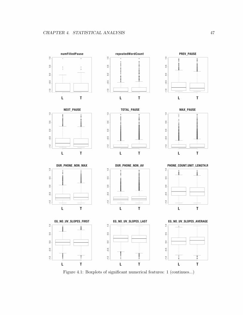
CHAPTER 4. STATISTICAL ANALYSIS 47
Figure 4.1: Boxplots of significant numerical features: 1 (continues...)
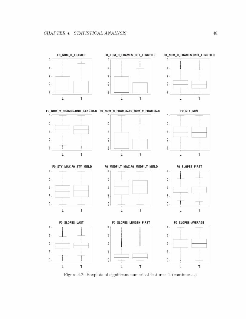
CHAPTER 4. STATISTICAL ANALYSIS 48
Figure 4.2: Boxplots of significant numerical features: 2 (continues...)
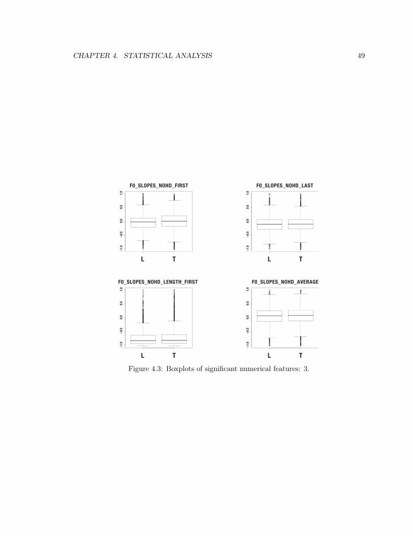
CHAPTER 4. STATISTICAL ANALYSIS 49
Figure 4.3: Boxplots of significant numerical features: 3.

Chapter 5. 50
Chapter 5
Analysis and Classification on the
Local Level
In this chapter, we take up classification on the local lie level. We begin by reporting
preliminary analyses of the data we have previously reported (Hirschberg et al., 2005; Benus
et al., 2006), and then describe our our initial results at classification, also first reported in
(Hirschberg et al., 2005). We then detail additional machine learning experiments on various
subsets of CSC Corpus features, showing substantial improvement over previously reported
results (Hirschberg et al., 2005) and over human performance, which was worse than chance
at an analogous task on the same data (Enos et al., 2006) (and see Chapter 10).
5.1 Preliminary Analyses
Initial lexical analyses of the CSC corpus involved using the lexical categorization program
Linguistic Inquiry and Word Count (LIWC) (Pennebaker, Francis & Booth, 2001).1,2 This
1These preliminary analyses using LIWC and the Dictionary of Affect in Language (see below) were
carried out by Jason Brenier and Cynthia Girand at the University of Colorado at Boulder, and we first
reported them in (Hirschberg et al., 2005).
2These initial analyses were carried out before the dataset was finalized, so that segment boundaries and
specific segments included in the analysis differed somewhat from those included in Chapter 4, for example
because boundaries of segment labels and exclusion criteria for offtalk were further refined.
CHAPTER 5. ANALYSIS AND CLASSIFICATION ON THE LOCAL LEVEL 51
program classifies words in a text according to a number of textual, semantic, and syntactic
categories; 68 were examined here. The LIWC dictionary of categories was developed by
hand and refined based on agreement by a panel of labelers. Categories hypothesized as
relevant for predicting subjects’ deceptive intent included emotion words, words denoting
cognitive activity, prepositions, pronouns. These hypotheses were based both on the litera-
ture (e.g. (Adams, 1996)) and on the intuitions of practitioners (Reid & Associates, 2000).
Our analyses suggested that deceptive speech has a greater proportion of positive emotion
words than does truthful speech (p = 0.0074). Other categories that appeared worthy of
further analysis are those of word count, and of lexical items relating to causation.
The early experiments with LIWC suggested that the examination of emotive content
is a promising avenue for deception detection in the CSC corpus. It is a basic premise of
deception research that a broad category of cues are emotional in nature (Ekman, 2001), and
there are suggestions in the literature that in general deceivers have different patterns of word
usage from speakers who are telling the truth (Newman, Pennebaker, Berry & Richards,
2003; Qin, Burgoon & Nunamaker, 2004; Zhou, Burgoon, Twitchell, Qin & Nunamaker,
2004). We thus attempted analysis using Whissell’s Dictionary of Affect in Language (DAL)
(Whissel, 1989). DAL addresses the emotional connotation of words along three dimensions:
pleasantness, activation, and imagery. The dictionary rates words on a continuous scale
[1, 3] for each of the three dimensions, with values determined by human judgment. Its 8742
entries, selected for inclusion by general corpus frequency, are claimed to cover about 90%
of an average English text.
We examined the distribution of DAL scores calculated by SU. We employed a test of
odds ratios; significance values for odds ratios are standardly obtained by computing z-scores
based on the estimated odds ratio and the corresponding standard error (Sheskin, 2007).
Preliminary findings suggested that pleasantness is the most promising factor in predicting
deception, that the minimum pleasantness score (computed by SU) appears to differ with
deception; this is consistent with the findings De Paulo et al. (2003) (See Table 2.1). Specif-
ically, analyses of odds ratios showed that for each unit increase in minimum pleasantness
score (on the three-point continuous scale described above), an utterance is 1.20 times more
likely to be deceptive (p = 0.001). When controlling for SU length, an utterance is 1.29
CHAPTER 5. ANALYSIS AND CLASSIFICATION ON THE LOCAL LEVEL 52
times more likely to be deceptive (p = 0.001) per unit increase in average pleasantness, and
for each unit increase in the standard deviation of pleasantness, an utterance is 54% less
likely to be deceptive (p = 0). Finally, for each unit increase in maximum pleasantness
score, an utterance tends to be 23% less likely to be deceptive (p = 0.085). No significant
effect was found for the imagery or activation dimensions.
Another claim in the literature is that filled pauses (e.g. um, uh) are perceived to sig-
nal discomfort with a topic or signal the beginning of a deceptive utterance (Tree, 2002; Vrij
& Winkel, 1991; Vrij, 2008), although there is little objective, empirical basis to support the
perception (DePaulo et al., 2003; Vrij, 2008). We examined filled and silent pauses in the
corpus in Benus et al. (2006). The CSC Corpus contains 3614 filled pauses, and in fact they
correlate more strongly with truthful than with deceptive speech in the local lie condition,
with χ2(1, N = 76, 635) = 20.52, p < 0.001. Turn-internal silent pauses also appear more of-
ten in truthful speech χ2(1, N = 74, 585) = 54.27, p < 0.001, and one-way ANOVA revealed
that silent pauses occurred more closely together in time in the TRUTH condition (F(1,
14954)=16,002, p<0.001). All of these findings regarding disfluencies seem to be consistent
with suggestions by practitioners (Reid & Associates, 2000) and findings in the empirical
literature (DePaulo et al., 2003) that deceptive speech is more careful or planned.
5.2 Preliminary Local Lie Classification With Ripper
The initial machine learning experiments on the corpus were performed with the Ripper rule-
induction classifier (Cohen, 1995) using the preliminary version of the feature set described
in Chapter 3. These experiments were performed on 9491 SUs, predicting TRUTH or
LIE on the local lie level. The baseline accuracy for this task, predicting majority class of
TRUTH, is 60.2% (this baseline and the number of labeled SUs in the dataset subsequently
changed slightly as offtalk was more narrowly defined and excluded). Data for all subjects
were pooled for these experiments. We divided the data 90%/10% into training and test
sets five times, trained on the former and tested on the latter, then averaged the results to
obtain the figures reported here.
We first examined the usefulness of the acoustic/prosodic features in distinguishing
CHAPTER 5. ANALYSIS AND CLASSIFICATION ON THE LOCAL LEVEL 53
TRUTH from LIE. Results for this feature-set averaged over our test sets were 61.5%
accuracy — only slightly above the baseline. Useful rules in this model included energy and
F0 features.
We next attempted prediction using models built exclusively from lexical features. Av-
erage accuracy over the five test sets was also around the baseline at 61.0%. Features
appearing in the rule-sets of these models included: the number of words repeated from the
interviewer’s queries, verb tense and the presence of filled pauses.
Combining both lexical and acoustic/prosodic features produced a classifier that per-
formed better than either feature-set alone, achieving an accuracy of 62.8% using all of the
lexical and acoustic features described above. This improvement was still rather modest
with respect to the baseline, however. In the rule sets produced in this experiment, the
acoustic/prosodic features markedly dominate the lexical features.
For these initial experiments, our speaker-dependent feature-set included subject id,
subject gender and the ratios described in Chapter 3. Including this feature-set with our
acoustic/prosodic and lexical feature-sets produced a considerable improvement, boosting
accuracy to 66.4% averaged over the five test sets. Sample rule-sets from these experiments
showed that speaker-dependent filled pause and cue phrase ratios, alone or combined with
acoustic energy and pitch features, produced the improvement. These initial results lent
support to the hypothesis that deceptive behavior in speech is a phenomenon with substantial
individual differences, and to our general expectation that sophisticated speech processing
techniques had promise for the deception detection task. It should be noted that in future
experiments we omitted the subject id feature, since we realized that uniquely identifying
individual subjects likely provided an unfair advantage to the classifier with respect to the
differing class distributions. Later in this chapter we will report experiments that omit this
feature and thus have greater methodological validity.
5.3 Local Lie Classification Using Combined Classifiers
We next examined whether or not improvements could be made by training separate local
lie classifiers on different feature sets and then combining the predictions of those systems as
CHAPTER 5. ANALYSIS AND CLASSIFICATION ON THE LOCAL LEVEL 54
features in a top level learner, or combiner (Graciarena, Shriberg, Stolcke, Enos, Hirschberg
& Kajarekar, 2006).3 Our hope was that the top-level classifier would weight the evidence
from each system and thus improve the accuracy of class prediction. We employed an
SVM with a radial basis function (RBF) kernel as the combiner. Specifically, scores from
an SVM system based on prosodic and lexical features were combined with scores from
a Gaussian mixture model (GMM) system based solely on acoustic features, resulting in
improved accuracy over the individual systems.
We first explored the performance of each system, and then the performance of the
combined system. Finally, we compared results from the prosodic-only SVM system using
features derived either from recognized words or from human transcriptions in order to assess
the potential effects of word-recognition errors.
5.3.1 Data
Each speaker’s SUs were randomly partitioned ten times (using ten different random seeds)
into splits of 90% and 10% for training and testing, respectively. Training and test data from
all speakers was pooled to form the final sets, resulting in a total of 8406 training SUs and
922 test SUs per run.
5.3.2 Prosodic-lexical SVM system
A support vector machine (SVM) classifier with a linear kernel was used with the prosodic-
lexical feature set. A total of 235 input features were used in the prosodic/lexical SVM
system, and 215 were used for the prosodic SVM system. We used the freely available
LIBSVM tool (Chang & Lin, 2001) in training and testing the SVMs. A zero mean and unit
standard deviation normalization was used for input features.4 Radial basis and polynomial
kernels were also tried, but we found that the linear kernel produced the best results.
3Martín Graciarena coordinated and implemented the bulk of the work reported in this section.
4There were very few cases of missing features in our CSC corpus. Missing feature values were replaced
by the mean of observed values for that feature.

CHAPTER 5. ANALYSIS AND CLASSIFICATION ON THE LOCAL LEVEL 55
5.3.3 Acoustic GMM system
The acoustic system attempted to discriminate truthful and deceptive speech using spectral
features, similarly to the approach used in speaker identification systems(Reynolds, 2002).
This system used spectral-based Mel cepstral features with energy, along with simple, double
and triple delta features, for a total of 52 features.
A Gaussian mixture model (GMM) classifier was trained using acoustic features; the total
number of Gaussians used was 2048. First, a boot GMM was trained using the expectation
maximization (EM) algorithm to maximize the likelihood of the model on the training data,
using all training data from both classes, TRUTH and LIE. Next, two separate GMMs
were created by adapting the boot GMM to the TRUTH data and to the LIE data,
using maximum a posteriori adaptation (MAP). This system makes a class prediction by
comparing the class posterior probabilities from each GMM for a given waveform (using
priors estimated from the training data).
5.3.4 Combiner SVM system
We evaluated whether combining scores from both systems would improve the classification
accuracy by combining prediction confidence scores from individual systems using an SVM
with an RBF kernel.
The score used from the acoustic GMM system was the ratio of the truthful GMM
posterior probability to the deceptive GMM posterior probability, an approach similar to
that used in speaker identification(Reynolds, 2002). We simulated a confidence score for the
SVM trained on prosodic-lexical features by taking the dot product of the kernel output of
the support vectors and the kernel output of the input vector, that is, the signed distance
(in kernel space) of the data point from the decision boundary.
The combiner was trained on a subset of the training data by splitting the training
data into two sets, called devtrain (80%) and devtest (20%). The prosodic-lexical SVM
and the acoustic GMM were trained using the devtrain data. Scores from each system
were then generated for the devtest data, and the combiner was subsequently trained
on that data.5 Predictions from each system were normalized to produce Z-scores. The
5For the purposes of comparing each independent system, the two systems were retrained on the full

CHAPTER 5. ANALYSIS AND CLASSIFICATION ON THE LOCAL LEVEL 56
Table 5.1: Accuracy of Single Systems and Combination Systems on the CSC Corpus (Gra-
ciarena et al., 2006).
System Accuracy (%)
Chance 60.4
(A) Acoustic GMM 62.1
(B) Prosodic SVM 62.7
(C) Prosodic/Lexical SVM 62.9
Systems A + B 64.4
Systems A + C 64.0
normalization parameters were computed from the devtrain data and were applied to the
test data.
5.3.4.1 Results
Table 5.1 presents results for the various systems tested. The chance result is that which
would be obtained by labeling every test instance TRUTH, the majority class.
From Table 5.1 we conclude that each individual system produces a gain over chance,
and that the prosody-based systems produce the largest gains. We reason that system A +
C was not better than system A + B because as the systems become more similar (i.e., via
the addition of lexical features) there are fewer distinct errors for the combiner to leverage.
A matched pairs test shows that difference in accuracy between chance and the combination
of systems A and B is significant (p < 0.05) as is the difference in accuracy between chance
and the combination of systems A and C (p < 0.10).
training set.

CHAPTER 5. ANALYSIS AND CLASSIFICATION ON THE LOCAL LEVEL 57
Table 5.2: Human Transcribed vs. Recognized Prosodic Systems. (Graciarena et al., 2006).
System Accuracy (%)
Chance 60.4
Prosodic SVM from Recognized Words 62.6
Prosodic SVM from Transcripts 62.8
5.3.5 Prosodic System from Recognized Words
Finally, we consider the impact of recognition error on classification accuracy. To do so,
we compare results from the prosodic-only SVM system reported above (that is, a system
using human transcribed true-words) with the results of a prosodic system whose features
are computed from automatically recognized words. SU boundaries from the previous ex-
periment were used, and recognition was performed with conversational telephone speech
recognizer adapted for full-bandwidth recordings (Stolcke et al., 2005). The procedure de-
scribed above for splitting training and test data was used. Since some short utterances
could not be recognized, the test sets contained 874 SUs while training sets contained 8104.
Table 5.2 shows the accuracy of both systems. These results reveal substantial robustness
of prosodic features in this application with respect to recognition errors (the difference is
not statistically significant). This is a useful result in that it suggests that whatever gain is
achieved from prosodic features can be achieved even without costly hand transcription.
5.4 In-depth Machine Learning Experiments
In this section, we report a series of machine learning experiments using the latest version of
the entire CSC Corpus feature set. We perform these experiments various subsets of features,
as noted below, using the entire local lie labeled SU set, a total of 9068 segments. The
aim of these experiments was three-fold: to compare the discriminative power of various
subsets of features; to assess the efficacy of broad classes of learning algorithms for this task
and the various feature sets; and to examine the models generated by successful learners in

CHAPTER 5. ANALYSIS AND CLASSIFICATION ON THE LOCAL LEVEL 58
order to infer which attributes of deceptive and non-deceptive speech are most helpful in the
detection task. The majority class baseline for this task, in all cases for the remainder of the
chapter, was 59.93%, guessing the majority TRUTH class. This baseline differs slightly
from that reported in earlier experiments (60.20% in the sections above), as subsequent to
those experiments we refined and implemented a more effective criterion for excluding offtalk
segments from the dataset.
Five learning algorithms are applied to each feature set. All of the learners are imple-
mented in Java by the Weka machine learning environment (Garner, 1995). Four broad
classes of learning algorithms are represented by five learners:
Naive Bayes A simple Bayesian classifier (John & Langley, 1995) which assumes that all
features are independent.
Ripper The Java JRip implementation of Ripper (Cohen, 1995), a propositional rule learner
with pruning.
c4.5 The Java J48 implementation of the c4.5 (Quinlan, 1986) decision tree learner.
Logistic Regression A multinomial logistic regression classifier (Cessie & van Houwelin-
gen, 1992) with a ridge estimator (to try to compensate for multicolinearity that may
exist in the predictor variables). We included logistic regression despite and because
of its similarity to the SVM: in our experience it sometimes performs better than an
SVM, and in cases where performance is similar, the logistic regression model is more
readily interpretable. In the case of the present task, logistic regression was successful
for only one data set, as we will note below.
SVM Platt’s (1998) SMO implementation of the support vector machine (SVM) (Boser,
Guyon & Vapnik, 1992).
Four feature sets are employed in the experiments presented in this chapter. Based on
the preliminary experiments reported above, and the insights gained during the subject-
dependent analyses of Chapter 8, we focus on the following feature sets:
Base This feature set includes the entire set of lexical features described in Appendix C
and all of the acoustic, and prosodic features examined in Chapter 4. These latter

CHAPTER 5. ANALYSIS AND CLASSIFICATION ON THE LOCAL LEVEL 59
comprise the raw acoustic/prosodic features enumerated in Appendix C (those whose
names do not reference a normalization scheme, e.g. ‘PNORM’); these features were
then normalized within speaker on the interval [−1, 1] using the uniform distribution,
as in Chapter 4.
Base + Subject-dependent This feature set includes the features of Base and the subject-
dependent features enumerated in Appendix C.
All This feature set includes the features of Base + Subject-dependent and all other
features enumerated in Appendix C.
Best 39 This is a subset of 39 features (listed in Table 5.6 on page 67) selected using Chi-
squared selection criteria from the Base + Subject-dependent set. We chose to per-
form feature selection on this set since, as will be shown below, the Base + Subject-
dependent set performed best of the three sets already described.
Several other feature sets were examined, but performance was such that it did not
warrant detailed reporting here: We attempted feature selection (a 54-feature set) from All,
but performance of the reduced set was worse than that of the original set; we attempted
using a greedy selection algorithm on Base + Subject-dependent, but the resulting set
performed worse than Best 39; and we constructed a set from those features that showed
significant differences in the statistical analyses of Chapter 4, but except as noted below in
the text, the classification results using that set were not statistically different from chance.
An additional approach that we attempted but found unsuccessful was to contextualize a
given segment with data from the prior segment and the segment that followed. That is, to
include in the data for a segment S the feature values for S − 1 and S + 1. We tried this
approach in varying combinations, but found that it had no effect on the learners except to
degrade performance with respect to training time.
All learners are applied to each feature set using 10 differently-seeded trials of 10-fold
cross validation for a total of 100 trials for each feature set/learner combination. In the
sections that follow we report accuracy (where the chance baseline is 59.93%), F-measure
with respect to both TRUTH and LIE, and standard error of the mean for all performance
measures (numerically in the tables and in figures via error bars representing ±1 S.E.).
CHAPTER 5. ANALYSIS AND CLASSIFICATION ON THE LOCAL LEVEL 60
5.4.1 Performance Metrics
In the results that follow, we report accuracy and F-measure with respect to both TRUTH
and LIE. For the purpose of evaluating the significance of the differences among feature
sets and classifiers with respect to accuracy, we offer two criteria. First, the standard error
of the mean is presented for all cross-validation experiments. This criterion is necessary,
but not sufficient, to establish significant differences. That is, if two results fall within the
range of the respective standard errors, the difference between them has a high likelihood
of occurring by chance; if they fall outside of this range, further information is required to
establish significance. For the purpose of more confidently establishing the significance of
differences among classifiers, we turn to the binomial model.6 For the purposes of applying
this model we begin by assuming a classifier that performs no better than the majority class
baseline (guessing TRUTH every time); that is, 59.93%. The binomial distribution has
expected value
E(X) = np
and standard deviation
S.D.(X) =√
np(1 − p) ,
where here p is the probability of membership in the class TRUTH (0.5993) and n is the
number of trials (907 for each test set). Applying our parameters to this distribution, we
compute a standard deviation of 14.76. By applying z-scores (effectively computing the
difference of two standard deviations from the expected value) we establish that a classifier
differing from the expected value by at least 3.3% would be significant at the 0.05 level.
This is an imperfect metric, since it assumes complete independence of samples, but it
is conservative: as the value of p decreases, the variance, and thus the critical value for
significance increases, and we have chosen for our value of p the prior probability of a given
sample’s being labeled TRUTH, a value smaller than the average accuracy of all of but one
of our classifier/feature-set combinations. Though imperfect, we will thus proceed under the
assumption that a difference in accuracy of at least 3.3% between two classifier/feature-set
combinations provides a reasonable assurance of significance.
6We are grateful to Dan Ellis for his assistance in selecting and implementing this evaluation criterion.

CHAPTER 5. ANALYSIS AND CLASSIFICATION ON THE LOCAL LEVEL 61
In addition to accuracy, we report F-measure with respect to both the TRUTH and
LIE classes. As Joshi (Joshi, 2002) points out, because F-measure does not have a prob-
abilistic interpretation, it does not lend itself to significance testing. That author suggests
a heuristic whereby a difference of 1% in F-measure between two classifiers is regarded as
significant. Although this seems a bit arbitrary, it again serves to contextualize our results
to some degree. In general, our discussions will exhibit greater interest in accuracy and in
F-measure for LIE than in F-measure for TRUTH. LIE is ostensibly the class of greater
interest, partly as it represents the minority class from the local lie perspective, and it
is thus harder to achieve a high score with regard to F-measure. We therefore hold that
increases in F-measure for LIE are indicative of more meaningful performance gains.
5.4.2 The Base feature set
Table 5.3 displays numerical results for the Base feature set. Results for the Ripper clas-
sifier are consistent with (and not statistically different from, even when accounting for
the slightly different baselines) results reported in previous sections using the entire lexical
and acoustic/prosodic feature sets. Those earlier experiments, using both Ripper and the
combiner SVM systems, provide the most similar basis for comparison. This comparable
performance is achieved in spite of the reduced size of the feature set (recall that the various
normalized versions of the acoustic/prosodic features were included in prior experiments).
We suggest that this is attributable to two causes: first, the full feature set evidences sub-
stantial multicolinearity7 among variables that represent differently-normalized versions of
the same value; second, our subsequent investigations (see, for example, Chapters 7 and
8) suggested that within-subject normalization should be helpful, since we have identified
many speaker-dependent aspects of deceptive speech.
As we will see in subsequent sections, c4.5 proved to be the best learner in most cases.
This is not exactly the case with the Base set, however. While c4.5 performs best with
respect to F-measure for LIE (by a difference of nearly 12.0 in the case of the SVM), c4.5,
SVM, and the logistic classifier all exceed the baseline by the 3.3% criterion established
in Section 5.4.1 for significance with respect to accuracy. Within that group none differ
7Probably better termed ‘redundancy’ with respect to its impact on rule-based or decision-tree learners.
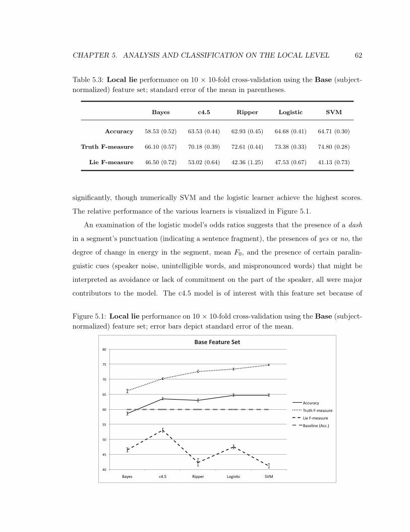
CHAPTER 5. ANALYSIS AND CLASSIFICATION ON THE LOCAL LEVEL 62
Table 5.3: Local lie performance on 10 × 10-fold cross-validation using the Base (subject-
normalized) feature set; standard error of the mean in parentheses.
Bayes c4.5 Ripper Logistic SVM
Accuracy 58.53 (0.52) 63.53 (0.44) 62.93 (0.45) 64.68 (0.41) 64.71 (0.30)
Truth F-measure 66.10 (0.57) 70.18 (0.39) 72.61 (0.44) 73.38 (0.33) 74.80 (0.28)
Lie F-measure 46.50 (0.72) 53.02 (0.64) 42.36 (1.25) 47.53 (0.67) 41.13 (0.73)
significantly, though numerically SVM and the logistic learner achieve the highest scores.
The relative performance of the various learners is visualized in Figure 5.1.
An examination of the logistic model’s odds ratios suggests that the presence of a dash
in a segment’s punctuation (indicating a sentence fragment), the presences of yes or no, the
degree of change in energy in the segment, mean F0, and the presence of certain paralin-
guistic cues (speaker noise, unintelligible words, and mispronounced words) that might be
interpreted as avoidance or lack of commitment on the part of the speaker, all were major
contributors to the model. The c4.5 model is of interest with this feature set because of
Figure 5.1: Local lie performance on 10 × 10-fold cross-validation using the Base (subject-
normalized) feature set; error bars depict standard error of the mean.

CHAPTER 5. ANALYSIS AND CLASSIFICATION ON THE LOCAL LEVEL 63
Table 5.4: Local lie performance on 10 × 10-fold cross-validation using the
Base + Subject-dependent feature set; standard error of the mean in parentheses.
Bayes c4.5 Ripper Logistic SVM
Accuracy 62.15 (0.48) 68.10 (0.52) 66.59 (0.51) 65.69 (0.42) 65.47 (0.50)
Truth F-measure 67.51 (0.49) 73.95 (0.46) 74.45 (0.51) 73.35 (0.36) 72.54 (0.43)
Lie F-measure 54.63 (0.56) 58.86 (0.69) 51.48 (1.08) 51.81 (0.61) 53.49 (0.67)
its performance with respect to LIE F-measure. An examination of this model shows that
broad categories of segments are demarcated by some of the paralinguistic features used in
the logistic model, that many mid-level rules make use of the lexical features mentioned
above along with positive and negative emotion words and topic, and that the leaves are
dominated by F0 (particularly slope) and energy features. As we noted, we will show that
c4.5 is generally the best performer for the feature sets we examined. That it performed
so much better here than the logistic and SVM learners with respect to LIE F-measure is
probably due to the fact that c4.5 is more readily able to capture complex relationships and
dependencies among the features, and these relationships will become more evident in the
following sections.
5.4.3 The Base + Subject-dependent feature set
Table 5.4 displays numerical results for the Base + Subject-dependent feature set. An
examination of this table and of the plot of Figure 5.2 reveals that c4.5 once again performs
best with respect to LIE F-measure by a substantial margin, and here performs best with
respect to accuracy as well, differing significantly from the baseline and the Bayesian classifier
but not from the other three learners. Performance on this feature set shows substantial
gains over the best performers on the Base set with respect to both measures of interest.
The c4.5 accuracy achieved here (68.10%) also improves upon the prior best results reported
in Section 5.2 for Ripper on the entire feature set — 66.4% vs. a baseline of 60.2%. Again,
we attribute these gains to the combination of the decision-tree learner with the normalized

CHAPTER 5. ANALYSIS AND CLASSIFICATION ON THE LOCAL LEVEL 64
Figure 5.2: Local lie performance on 10 × 10-fold cross-validation using the
Base + Subject-dependent feature set; error bars depict standard error of the mean.
features.
An examination of the tree learned for this feature set shows a heavy use of features
capturing energy and pitch changes (slopes and number of rising/falling frames) in the leaf
nodes, along with some lexical features, particularly positive and negative emotion words,
part-of-speech tags (past tense and third person) and negations. Lexical features also ap-
pear as mid-level rules, as do paralinguistic features such as laughter and mispronunciation.
TOPIC appears as a feature with some frequency in combination with various lexical fea-
tures, possibly signaling differing lexical strategies depending on topic. The addition of the
subject-dependent features has clearly improved performance, and these features generally
appear as top-level nodes. We interpret the appearance of the subject-dependent and TOPIC
features in the higher-level nodes as suggesting that these features help to divide speakers
by broad categories with respect to their deceptive behaviors, which are then differentiated
at the leaf nodes by lexical and acoustic features. This is a pattern that appears throughout
the experiments reported here.

CHAPTER 5. ANALYSIS AND CLASSIFICATION ON THE LOCAL LEVEL 65
Table 5.5: Local lie performance on 10 × 10-fold cross-validation using All features; stan-
dard error of the mean in parentheses.
Bayes c4.5 Ripper Logistic SVM
Accuracy 59.49 (0.48) 67.39 (0.43) 66.63 (0.52) 66.09 (0.42) 66.07 (0.46)
Truth F-measure 67.43 (0.43) 73.22 (0.37) 74.50 (0.50) 73.56 (0.36) 73.49 (0.41)
Lie F-measure 46.37 (0.76) 58.28 (0.62) 51.56 (0.90) 52.69 (0.63) 52.82 (0.62)
5.4.4 The All feature set
The addition, as described above, of the remainder of the normalized features that comprise
the entire feature set has little effect on performance. Performance of all of the learners (Ta-
ble 5.5) is not statistically different from performance on the Base + Subject-dependent
set, except for considerably poorer performance by the Naive Bayes learner, presumably
due to the redundancy of features. A comparison of plots for performance on this set (Fig-
ure 5.3) with performance on Base + Subject-dependent (Figure 5.2) shows that relative
performance among the four learners (represented by the contour of the plot lines) is quite
similar.
As c4.5 is again the best learner, we examine the decision tree produced for this feature
set. This tree differs from that for Base + Subject-dependent in that, along with subject
dependent features, some of the normalized energy features, such as EG_RAW_MIN_EG_PNORM
appear as top-level rules. The leaves are dominated by lexical features similar to those in
the previous tree we described (POS-tags and positive and negative emotion words) but
contain some F0 and energy slope or change features, as did previous models. The most
interesting aspect of trials on All features, however, is the lack of improvement over the
Base + Subject-dependent set; we will examine this further in our discussion below.
5.4.5 The Best 39 feature set
To this point, the most interesting aspect of these experiments has been the performance
of the Base + Subject-dependent set, which exceeded previous results on the corpus
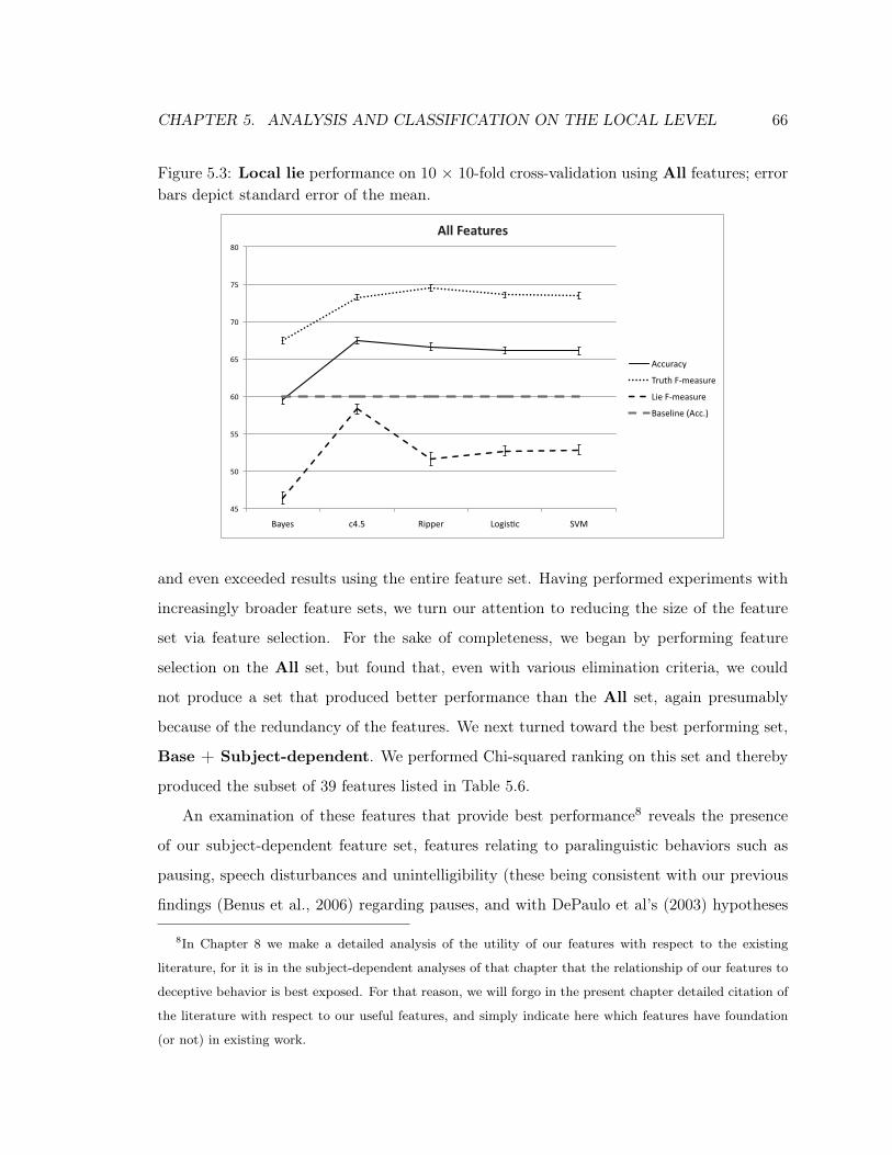
CHAPTER 5. ANALYSIS AND CLASSIFICATION ON THE LOCAL LEVEL 66
Figure 5.3: Local lie performance on 10 × 10-fold cross-validation using All features; error
bars depict standard error of the mean.
and even exceeded results using the entire feature set. Having performed experiments with
increasingly broader feature sets, we turn our attention to reducing the size of the feature
set via feature selection. For the sake of completeness, we began by performing feature
selection on the All set, but found that, even with various elimination criteria, we could
not produce a set that produced better performance than the All set, again presumably
because of the redundancy of the features. We next turned toward the best performing set,
Base + Subject-dependent. We performed Chi-squared ranking on this set and thereby
produced the subset of 39 features listed in Table 5.6.
An examination of these features that provide best performance8 reveals the presence
of our subject-dependent feature set, features relating to paralinguistic behaviors such as
pausing, speech disturbances and unintelligibility (these being consistent with our previous
findings (Benus et al., 2006) regarding pauses, and with DePaulo et al’s (2003) hypotheses
8In Chapter 8 we make a detailed analysis of the utility of our features with respect to the existing
literature, for it is in the subject-dependent analyses of that chapter that the relationship of our features to
deceptive behavior is best exposed. For that reason, we will forgo in the present chapter detailed citation of
the literature with respect to our useful features, and simply indicate here which features have foundation
(or not) in existing work.
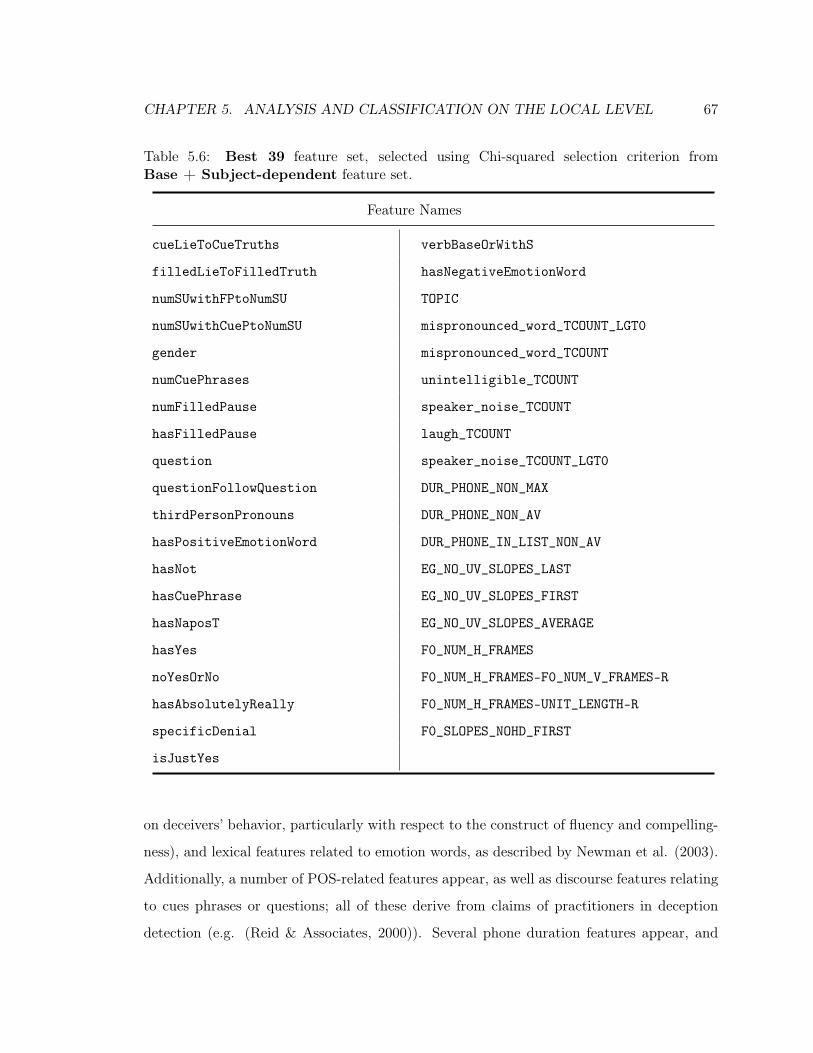
CHAPTER 5. ANALYSIS AND CLASSIFICATION ON THE LOCAL LEVEL 67
Table 5.6: Best 39 feature set, selected using Chi-squared selection criterion fromBase + Subject-dependent feature set.
Feature Names
cueLieToCueTruths verbBaseOrWithS
filledLieToFilledTruth hasNegativeEmotionWord
numSUwithFPtoNumSU TOPIC
numSUwithCuePtoNumSU mispronounced_word_TCOUNT_LGT0
gender mispronounced_word_TCOUNT
numCuePhrases unintelligible_TCOUNT
numFilledPause speaker_noise_TCOUNT
hasFilledPause laugh_TCOUNT
question speaker_noise_TCOUNT_LGT0
questionFollowQuestion DUR_PHONE_NON_MAX
thirdPersonPronouns DUR_PHONE_NON_AV
hasPositiveEmotionWord DUR_PHONE_IN_LIST_NON_AV
hasNot EG_NO_UV_SLOPES_LAST
hasCuePhrase EG_NO_UV_SLOPES_FIRST
hasNaposT EG_NO_UV_SLOPES_AVERAGE
hasYes F0_NUM_H_FRAMES
noYesOrNo F0_NUM_H_FRAMES-F0_NUM_V_FRAMES-R
hasAbsolutelyReally F0_NUM_H_FRAMES-UNIT_LENGTH-R
specificDenial F0_SLOPES_NOHD_FIRST
isJustYes
on deceivers’ behavior, particularly with respect to the construct of fluency and compelling-
ness), and lexical features related to emotion words, as described by Newman et al. (2003).
Additionally, a number of POS-related features appear, as well as discourse features relating
to cues phrases or questions; all of these derive from claims of practitioners in deception
detection (e.g. (Reid & Associates, 2000)). Several phone duration features appear, and
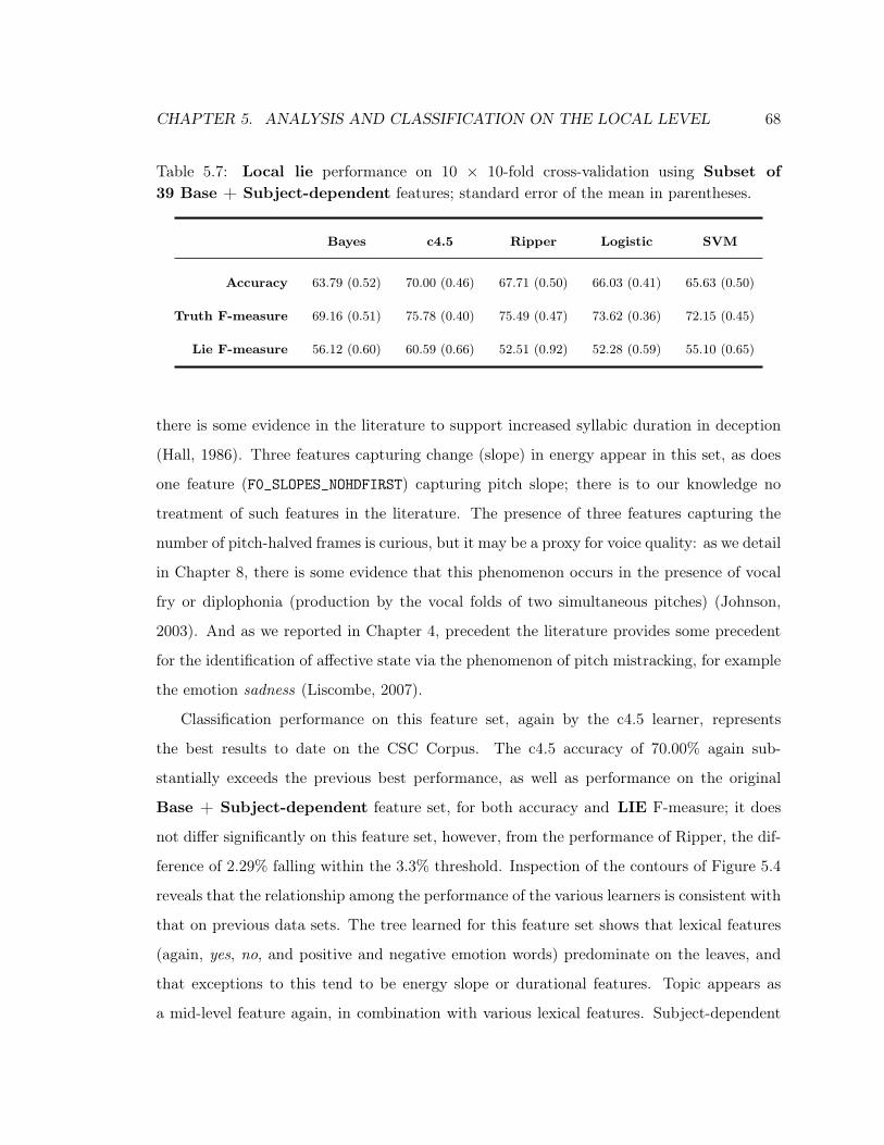
CHAPTER 5. ANALYSIS AND CLASSIFICATION ON THE LOCAL LEVEL 68
Table 5.7: Local lie performance on 10 × 10-fold cross-validation using Subset of
39 Base + Subject-dependent features; standard error of the mean in parentheses.
Bayes c4.5 Ripper Logistic SVM
Accuracy 63.79 (0.52) 70.00 (0.46) 67.71 (0.50) 66.03 (0.41) 65.63 (0.50)
Truth F-measure 69.16 (0.51) 75.78 (0.40) 75.49 (0.47) 73.62 (0.36) 72.15 (0.45)
Lie F-measure 56.12 (0.60) 60.59 (0.66) 52.51 (0.92) 52.28 (0.59) 55.10 (0.65)
there is some evidence in the literature to support increased syllabic duration in deception
(Hall, 1986). Three features capturing change (slope) in energy appear in this set, as does
one feature (F0_SLOPES_NOHDFIRST) capturing pitch slope; there is to our knowledge no
treatment of such features in the literature. The presence of three features capturing the
number of pitch-halved frames is curious, but it may be a proxy for voice quality: as we detail
in Chapter 8, there is some evidence that this phenomenon occurs in the presence of vocal
fry or diplophonia (production by the vocal folds of two simultaneous pitches) (Johnson,
2003). And as we reported in Chapter 4, precedent the literature provides some precedent
for the identification of affective state via the phenomenon of pitch mistracking, for example
the emotion sadness (Liscombe, 2007).
Classification performance on this feature set, again by the c4.5 learner, represents
the best results to date on the CSC Corpus. The c4.5 accuracy of 70.00% again sub-
stantially exceeds the previous best performance, as well as performance on the original
Base + Subject-dependent feature set, for both accuracy and LIE F-measure; it does
not differ significantly on this feature set, however, from the performance of Ripper, the dif-
ference of 2.29% falling within the 3.3% threshold. Inspection of the contours of Figure 5.4
reveals that the relationship among the performance of the various learners is consistent with
that on previous data sets. The tree learned for this feature set shows that lexical features
(again, yes, no, and positive and negative emotion words) predominate on the leaves, and
that exceptions to this tend to be energy slope or durational features. Topic appears as
a mid-level feature again, in combination with various lexical features. Subject-dependent

CHAPTER 5. ANALYSIS AND CLASSIFICATION ON THE LOCAL LEVEL 69
Table 5.8: Local lie performance on 10 × 10-fold cross-validation: Best learner(s) for
each feature set; standard error of the mean in parentheses.
Base | c4.5 Base | Logistic Subj-Base | c4.5 All | c4.5 39 Feats | c4.5
Accuracy 63.53 (0.44) 64.68 (0.41) 68.10 (0.52) 67.39 (0.43) 70.00 (0.46)
T F-measure 70.18 (0.39) 73.38 (0.33) 73.95 (0.46) 73.22 (0.37) 75.78 (0.40)
L F-measure 53.02 (0.64) 47.53 (0.67) 58.86 (0.69) 58.28 (0.62) 60.59 (0.66)
features again generally appear as top-level nodes.
5.4.6 Discussion
Table 5.8 consolidates the best learners for each feature set. The relationship among the
learners is perhaps best represented by Figure 5.5, where it can be seen that c4.5 along with
the 39 Best set outperforms all other learners and feature sets with respect to F-measure.
Numerically, it also outperforms the other combinations with respect to accuracy, although
Figure 5.4: Local lie performance on 10 × 10-fold cross-validation using Subset of
39 Base + Subject-dependent features; error bars depict standard error of the mean.
CHAPTER 5. ANALYSIS AND CLASSIFICATION ON THE LOCAL LEVEL 70
it does not differ by the critical value of 3.3% from the Base + Subject-dependent or All
feature sets. There are several observations that follow from the performance reported here.
First, these results provide clear support for the feasibility of detecting deceptive speech
better than chance and substantially better than human hearers, who performed worse than
chance on an analogous task on the same data (see Chapter 10). Second, the performance
of these classifiers begins to provide some insight into the nature of the task. That the
decision tree learner consistently outperformed other learners suggests that deceptive speech
is complex, requiring the modeling of multiple relationships among features in order to
classify it with any success. This contention is supported by the poor performance of the
Naive Bayes learners, which are hampered by their inability to model dependencies among
variables. It is further supported by the poor performance with respect to LIE F-measure
in the one case where the logistic learner performed best with respect to accuracy. We
mentioned in the introduction to these experiments that the logistic learner also performed
best on one other data set: that composed solely of the significant features from the analyses
of Chapter 4. Logistic regression achieved 61.87% accuracy on these 28 features (S.E. 1.24),
besting the other learners. We speculate that the fact that the logistic learner performed
best and that that best performance was relatively poor were due to the same fact: that
this group of features was selected specifically because of the univariate significance of each
feature with respect to deception. Logistic regression was thus best able to capture what
discriminative power exists in each of these features, but by definition that discriminative
power did not capture the complex relationships available to be mined in the broader feature
set. As an aside, we also attempted to employ boosting (Freund & Schapire, 1995) along
with c4.5 on the better performing feature sets. The boosted learners performed consistently
worse, suggesting that we are perhaps reaching the threshold of discriminative power inherent
in the current feature sets.
It is also of interest that the All feature set provided the third-best performance overall.
(In addition, it of course took substantially longer to train a model using this larger set
— 33.40 minutes on average for c4.5, as compared with an average of 3.17 minutes for
the best-performing 39 Best set on identical linux machines.) As we described above, we
believe this is partly due to the redundancy of the data with respect to various normalization

CHAPTER 5. ANALYSIS AND CLASSIFICATION ON THE LOCAL LEVEL 71
Figure 5.5: Local lie performance on 10 × 10-fold cross-validation Best learner(s) for
each feature set; error bars depict standard error of the mean.
schemes. There is a second factor that also may be at play here, however. Many of these
normalization schemes were developed for the purpose of speaker identification tasks, and
thus apply normalization over the entire data set, as would be expected when the domain
requires comparison of the behavior of one speaker to that of another. Since, however,
deception detection increasingly seems to be a within-subject discrimination task, it is not
surprising that these normalized features do not provide additional discriminative power.
This argument is bolstered by the observation that the best performance to date has been
on a subset of features (Best 39) that reflect within-speaker normalization.
5.5 Conclusions
We have detailed in this chapter a variety of analyses and machine learning experiments with
respect to local lie classification of the CSC Corpus. In these analyses and experiments, we
have shown evidence for the existence of a variety of speech phenomena that cue deception,
and we have produced progressive increases with respect to performance measures of interest.
Additionally our classifiers have substantially outperformed human labelers on an analogous

CHAPTER 5. ANALYSIS AND CLASSIFICATION ON THE LOCAL LEVEL 72
task using the same data (see Chapter 10). These results offer ample support for the use
of speech processing techniques for the classification of local lies in the CSC Corpus and
provide motivation for continued work in this regard.
Chapter 6. 73
Chapter 6
Classification of Global Lies
In this chapter, we focus on detecting a speaker’s more general intention to deceive, i.e., to
perpetrate what we term global lies, as introduced in Chapter 3. We do so by examining
certain systematically identifiable segments — called here critical segments — that may
be more emotionally or cognitively charged than segments from the general corpus. These
segments are of interest because they bear propositional content that is directly related to the
topics of most interest in the mock interrogation paradigm used in the corpus; classification
of such segments is thus particularly important. Results reported here substantially exceed
human performance at the task of global lie classification, which we take up in Chapter 10
and have previously reported (Enos et al., 2006). Interestingly, models generated using
these segments employ features consistent with hypotheses in the literature (DePaulo et al.,
2003) and the expectations of practitioners (Reid & Associates, 2000) about spoken cues to
deception.
These findings are of interest on a number of fronts. First, they suggest that there may
be a speech analog to what psychologists who study behavioral and facial cues to deception
call hot-spots, events in which relevant emotion is particularly observable and can thus
be more easily detected (Adelson, 2004; Frank, 2005). Second, such findings can guide the
design of future data collection paradigms and real-world approaches, since interviewing
techniques might be optimized to induce the subject to produce more critical segments.
Finally, continued work on automatic detection can be guided by the general principle that
certain kinds of subject responses are more susceptible to detection, and that methods should

CHAPTER 6. CLASSIFICATION OF GLOBAL LIES 74
be developed to identify and examine these sorts of responses.
6.1 Global Lies Via Critical Segments
Work by psychologists studying behavioral and facial cues to deception (Adelson, 2004;
Frank, 2005) suggests that certain events in interviews, termed hot-spots, are particularly
useful in determining whether a subject is telling the truth. In considering likely candidates
for such hot-spots, we realized that the most likely segments were those whose proposi-
tional content corresponded to the global lie level of deception in our data. We additionally
hoped to find that certain segments of speech that deal directly with the most salient topics
of the speaker’s deception are more easily classified than deceptive statements in the corpus
at large. Presumably, such segments will be both emotionally charged — potentially result-
ing in stronger prosodic and acoustic cues — and cognitively loaded — potentially resulting
in more lexical cues to deception.
In the present work, we attempted to develop systematic rules to isolate potential hot-
spots, which in the speech domain we term critical segments. These rules are based
on two simple hypotheses about the nature of critical segments:
1. Critical segments will occur when the propositional content of the segment relates
directly to the most salient topics of the interview.
2. Critical segments will occur when subjects are directly challenged to explain their
claims with regard to salient topics of the interview.
In what follows, we explain our approach to operationalizing our hypotheses (Sec-
tion 6.2), and report results obtained by experiments performed on the data thus extracted
from the CSC Corpus (Section 6.3).
As we described in Chapter 2, a human baseline for the general deception-detection task
can be found in a the meta-analysis by Aamodt and Mitchell (2006) of the results of 108
studies of human deception detection. The majority of studies employed college students,
who scored on average 54.22% compared to a baseline of 50%. Police and federal officers also
performed near chance. A meta-analysis by Bond and DePaulo likewise estimates human
deception detection accuracy at around 54% in the general case.

CHAPTER 6. CLASSIFICATION OF GLOBAL LIES 75
In Chapter 10 we will describe in detail a perception study in which human subjects
attempted to discern between truth and deception in the CSC Corpus. That work provides
a roughly analagous human baseline with respect to the global lie detection task of the
present chapter. In the perception study, human subjects scored on average an accuracy of
47.76%, against a chance baseline of 62.55%; that is, humans performed substantially worse
than chance at a task analagous to that reported in the present chapter.
6.2 Methods and Materials
We performed machine learning classification experiments on critical segments identified
in the CSC corpus. These were performed using implementations of bagging (Breiman,
1996), AdaBoost (Freund & Schapire, 1995), and c4.5 (Quinlan, 1986) provided by Weka
and the Weka Java API (Garner, 1995). Feature selection was performed on the full CSC
Corpus feature set during the current experiments; features used are described in further
detail in Section 6.3.
6.2.1 Selection of critical segments
Critical segments were selected by hand from the full set of segments (EARS slash units
or SUs (NIST, 2004)) using the following rules:
1. Include segments that are responses to questions that directly ask the subject for
his/her score on a particular section.
2. Include segments that respond to immediate follow-up questions requesting a justifi-
cation of the claimed score, when such a question is posed by the interviewer.
3. Omit everything else.
Here is an example of a subject segment (labeled (S)) that corresponds to Rule 1:
(I) And what was your score exactly on that section?
(S) I got excellent, which was, um, pretty good.

CHAPTER 6. CLASSIFICATION OF GLOBAL LIES 76
The interviewer frequently posed a follow-up question requesting immediate justification of
the score claimed by the subject, as described in Rule 2. Responses to such questions were
included:
(I) Why do you think you did so well on that section?
(S) Um my- first of all my grandmother was a really good cook.
Often, a subject used multiple adjacent SUs in a response that corresponded to Rules 1 or
2. In such a case, all segments representing the response were included:
(I) So we’ll move on now to what we’re calling the civics section. How did you do on that
section?
(S) Uh I d- you know alright.
(S) Not great.
(S) Fair.
Finally, many subject segments did not correspond to either Rules 1 or 2 because they
were not produced in response to questions of the two genres described above. Such segments
were omitted for this analysis, e.g.:
(S) I went to this in- Indian restaurant my parents call Tamarind’s.
From the corpus of 9068 SUs, we thus produced two sets of critical segments: one
set of 465 based only on Rule 1 (termed Critical) and one set of 675 critical segments
based on Rules 1 and 2 (termed Critical-Plus). Feature selection was employed to reduce
the full feature set to 22 features for the Critical set and 56 for the Critical-Plus set.
6.2.2 Coping with skewed class distributions
It is well known that classification algorithms — particularly those using decision trees,
such as c4.5 (Quinlan, 1986) — can be negatively affected by datasets in which the class
distribution is skewed (Chawla, 2003; Drummond & Holte, 2003; Hoste, 2005). In simple
terms, this results in a bias on the part of the induced decision tree towards the majority
class because of the “over-prevalence” (Chawla, 2003) of majority class examples.
The CSC Corpus is such a dataset with respect to critical segments. The present
sets of critical segments contain a majority of LIE examples: (67.5% for Critical, 62%

CHAPTER 6. CLASSIFICATION OF GLOBAL LIES 77
for Critical-Plus). Because initial classification results on the natural class distribution
were poor but exceeded chance, we hypothesized that adjusting the class imbalance might
allow the learner to induce more effective rules. We follow a commonly used approach to
adjust the imbalance.
In this approach, termed under-sampling (Drummond & Holte, 2003),1 examples from
the majority class are eliminated in order to create a balanced distribution. For the Critical-
Plus dataset, combined training/test sets of 508 examples were used.2 Under-sampled
training/test sets were created as follows: for each of 10 training/test sets, randomly select
50 examples (25 TRUTH, 25 LIE) for the test set; from the remaining examples, randomly
select 458 (229 TRUTH, 229 LIE) for the test set. An analogous approach was used with
the Critical dataset, producing sets of 272 training and 30 test examples.
For each dataset, the above procedure was repeated 10 times with different random
seeds to account for the exclusion of some data; results reported here thus reflect average
performance on 100 individual training/test sets for each dataset.
6.3 Results and Discussion
In Table 6.1 we report classification results for the two datasets, both for the original samples
(using 10-fold cross-validation) and for the under-sampled datasets, using 100 random trials
as described in Section 6.2.2. Both raw accuracy and improvement relative to chance are
reported. Given the difference in baselines, the relative scores represent the best basis for
comparison since these scores are normalized with respect to the baseline chance accuracy,
which varies among the configurations of the data. Performance on the original samples is
poor but exceeds chance: 5.8% relative to chance for the Critical-Plus dataset, 1.6% for the
Critical dataset. Results for the under-sampled datasets show 22.2% relative improvement
for the Critical-Plus set and 23.8% relative improvement for the Critical set. This lends
support to our hypothesis with respect to the skew of the distribution: in cases where the
over-prevalence of one class interferes with c4.5’s modeling, resampling can render the learner
1Under-sampling is generally preferable to over-sampling; see (Drummond & Holte, 2003) for details.
2The total number of examples available after subtracting the 167 “excess” LIE examples is 508.

CHAPTER 6. CLASSIFICATION OF GLOBAL LIES 78
Table 6.1: Accuracy Detecting Global Lies
Relative
Dataset Improvement Accuracy Baseline
Human global lie performance -23.3% 47.76 62.55
Critical-Plus 5.8% 65.6 62.0
Critical 1.6% 68.6 67.5
Critical-Plus / Under-sampled 22.2% 61.1 50.0
Critical / Under-sampled 23.8% 61.9 50.0
more capable of producing useful rules.(Chawla, 2003; Hoste, 2005)
There are no previous machine learning results for classification of global lies on the
CSC Corpus to provide a standard for comparison. As we described above, however, some
context is provided by the performance of humans at the analogous task of labeling global
lies with respect to each section of the interview: 32 human listeners scored on average
47.76% versus a chance baseline of 62.55%.
An interesting aspect of these results is that performance is slightly better for the
Critical dataset than for the Critical-Plus dataset, despite the smaller size of the former
(272 training examples in each trial, versus 414). We suspect that this difference is due to
the increased cognitive and emotional stakes of the questions involved: The Critical dataset
contains only subject segments that respond directly to the interviewer’s most salient ques-
tions (e.g. “What was your score on section X?”); the additional segments of the Critical-
Plus dataset include segments that contextualize that question but do not respond directly
to it. It is possible that the latter differ enough with respect to emotional and cognitive load
to produce a less effective learner when included with the smaller Critical set.

CHAPTER 6. CLASSIFICATION OF GLOBAL LIES 79
6.3.1 Relevant features
The sets of features employed here, obtained using Weka’s implementation of Chi-squared
ranking feature selection, are displayed in Tables 6.2 and 6.3. Because the bagging/boosting
approach used here in 100 trials per dataset produced a large number of c4.5 decision trees,
it is impractical to give an exhaustive description of the features employed in the models.
We can, however, make some general observations about features that applied to a large
number of cases in the induced trees.
Many of the rules induced from the current dataset paint a very plausible picture of the
correlates of deception and one that is consistent with previous literature. First, lexical cues
that speak to emotional state, such as the presence of negative or positive emotion words
(Whissel, 1989; Newman et al., 2003), appear prominently. In particular, the presence of
positive emotion words correlates positively with truth in many of the models produced.
Likewise, many decision trees include rules based on features that could be interpreted to
relate to the quality of being “compelling” (DePaulo et al., 2003). The use of such assertive
terms as yes or no, for example, serves as a cue to deception in the models produced.
Likewise, the presence of a specific, direct denial that the subject is lying (e.g. “I did not”)
is used in many rules as a cue to truth. This feature in particular has been cited by law
enforcement practitioners as a cue to deceit (Reid & Associates, 2000), but we are unaware
of previous evidence in the scientific deception literature that supports this claim. The
presence of qualifiers (such as absolutely or really) is employed as a cue to deception in the
models; this again is a feature gleaned from conversations with practitioners. Filled pauses
appear as a cue to truth in many rules produced; this is consistent with an analysis of
filled pauses in the CSC Corpus reported in Chapter 5 and in our prior publication (Benus
et al., 2006). Self-repairs appear in numerous rules as a cue to truth; this is consistent with
the finding of DePaulo et al. (2003) that liars exhibit fewer ordinary imperfections in their
speech. Finally, various energy features (captured using a number of normalization schemes
described in Appendix C and by Shriberg et al. (Shriberg & Stolcke, 2004)) are employed
in complicated rules that suggest that extreme values for energy — either high or low —
correlate with deception. This is consistent with suggestions in the literature (O’Sullivan &
Ekman, 2004) that a subject’s deviation from his or her baseline behavior is a useful cue to

CHAPTER 6. CLASSIFICATION OF GLOBAL LIES 80
Table 6.2: Features used in classifying the Critical-Plus data set.
Feature Names
cueLieToCueTruths hasPastParticipleVerb
numFilledPause dash_slash_TCOUNT
hasFilledPause dash_slash_TCOUNT_LGT0
filledLieToFilledTruth mispronounced_word_TCOUNT_LGT0
numSUwithFPtoNumSU unintelligible_TCOUNT_LGT0
verbBaseOrWithS speaker_noise_TCOUNT_LGT0
hasNot breath_TCOUNT_LGT0
hasPositiveEmotionWord laugh_TCOUNT_LGT0
hasWe TOTAL_PAUSE
noYesOrNo MAX_PAUSE
hasI TOTAL_PAUSE-UNIT_LENGTH-R
specificDenial PAUSE_COUNT
hasNo DUR_PHONE_NON_MAX
hasAbsolutelyReally DUR_PHONE_IN_LIST_NON_MAX
PUNCT UNIT_LENGTH
hasNaposT PHONE_ZN_COUNT_LONG
verbWithIng PHONE_SPZN_COUNT_LONG
hasSelfRepair PHONE_IN_LIST_ZN_COUNT_LONG
hasYes EG_RAW_MIN_EG_DNORM
hasPastTenseVerb EG_RAW_MIN_EG_NNORM
gender EG_NO_UV_NUM_F_FRAMES
possessivePronouns EG_RAW_MEAN_EG_PNORM
hasNegativeEmotionWord EG_NO_UV_SLOPES_NUM_CHANGES
thirdPersonPronouns EG_RAW_MIN_EG_ZNORM
hasCuePhrase F0_SLOPES_LENGTH_FIRST
hasContraction F0_NUM_V_FRAMES
questionFollowQuestion F0_SLOPES_NOHD_LENGTH_LAST-UNIT_LENGTH-R
question F0_SLOPES_LENGTH_LAST-UNIT_LENGTH-R
deception. Interestingly, although some studies have shown a correlation between increased
F0 and deception (e.g. (Streeter et al., 1977)), F0 features do not appear prominently in
most of the rules induced here. One notable exception is that a number of F0 slope features
do appear in rules induced on the Critical-Plus dataset; we hesitate to make inferences

CHAPTER 6. CLASSIFICATION OF GLOBAL LIES 81
Table 6.3: Features used in classifying the Critical dataset.
Feature Names
cueLieToCueTruths PUNCT
hasFilledPause hasNaposT
numSUwithFPtoNumSU hasSelfRepair
verbBaseOrWithS hasYes
hasNot gender
hasPositiveEmotionWord hasCuePhrase
noYesOrNo dash_slash_TCOUNT_LGT0
hasI unintelligible_TCOUNT_LGT0
specificDenial breath_TCOUNT_LGT0
hasNo EG_RAW_MIN_EG_DNORM
hasAbsolutelyReally EG_RAW_MIN_EG_NNORM
about the nature of the correlation, however, since these features are generally embedded
in complicated subtrees. A difference between our two datasets is that the presence of past
tense verbs appears to correlate with deception in the Critical-Plus dataset, while it is
not employed in the Critical set.
6.3.2 Other observations
One further aspect of the skewed class distribution should be addressed here. Table 6.1
reports results for the original distribution (skewed) of both datasets and for the under-
sampled (unskewed) distribution. We also attempted to apply the model trained on the
unskewed data to test data skewed in the original class distribution, and in this we were
unsuccessful, achieving performance no better than chance. This was disappointing, but
gives rise to several observations. First, it is possible that the combination of the mismatch
in prior distributions between the train and test sets with the relatively small sample size
served to hamper the performance of the models. Second, these results point to a difficult
methodological issue in automatic deception detection research (and in other domains, such
as emotion detection, where priors are unknown and data are sparse): although models must
be trained using a fair amount of data from all classes of interest, the real-world distribution

CHAPTER 6. CLASSIFICATION OF GLOBAL LIES 82
of lies in any particular domain is likely sparse, but more importantly unknown. This is
in contrast to other sorts of speech and language processing tasks, where at the very least
the prior distributions of the phenomena of interest can be ascertained with some certainty.
Nevertheless, the work reported in this chapter represents some success, both with respect
to the performance achieved in this first attempt to detect global lies , and to the inter-
esting feature usage we described in Section 6.3.1. However, these observations regarding
the class distribution of the data seem to suggest that future research must focus further on
the issues of both class distribution and sparse phenomena when designing paradigms and
experiments.
Keeping this in mind, we have nevertheless shown that a more powerful classifier can be
trained using resampling techniques that compensate for the corpus’ skewed class distribu-
tions. The substantially improved performance indicates that the learner is better able to
infer more useful rules when the present data are distributed evenly — and more importantly
that such rules exist.
6.4 Conclusions and Future Work
The work reported here uses systematically identifiable critical segments to detect de-
ception on the global lie level in the CSC Corpus. Results substantially exceed human
performance at a similar task. This finding can guide future research on a number of fronts.
First, future paradigms can be designed to optimize subjects’ production of critical seg-
ments. For example, interviewers can be instructed to focus primarily on questions that
require direct assertions about the most salient facts of the paradigm.
Other approaches to detecting global lies merit exploration as well, and we envision a
variety of such approaches. For example, one strategy might entail a two-stage approach, first
attempting to classify individual segments, such as SUs with respect to their membership in
a global lie section, and then taking the majority of such segment labels (possibly adjusted
by some threshold) as the prediction for the entire global lie section. A second approach
could entail classification using simple n-gram language models, creating one such model
for deceptive speech and one for truthful speech, and classifying unknown sections via a

CHAPTER 6. CLASSIFICATION OF GLOBAL LIES 83
likelihood ratio or analogous technique.

PART III. 84
Part III
Speaker and Group Dependent
Analyses
Chapter 7. 85
Chapter 7
Motivations and Preliminary Speaker
Dependent Analyses
Early analyses of the CSC Corpus and the results of our preliminary experiments suggested
the existence of speaker differences with respect to cues to deception. A review of the
literature, along with conversations with practitioners, likewise suggested that the area of
individual differences in the deception domain in general and in deceptive speech in particular
are fertile areas for exploration.
We have undertaken here to examine the phenomenon of speaker differences on a number
of levels. Our initial motivating experiments involved speaker-dependent logistic regression
analyses of six simple pitch and energy features. We next consider a direct statistical analy-
sis, by speaker, of our lexical features and of our base set of acoustic and prosodic features,
and certain other numerical features. In this analysis, we set out to determine what features
vary significantly for each subject across the local truth and local lie conditions.1 A re-
lated analysis produces a graphical representation of the similarities that exist among certain
speakers with respect to the significance of acoustic and prosodic features, and we attempt
to infer some broad categories of speakers in terms of prosodic and acoustic behavior in the
TRUTH and LIE conditions. In related work, we consider the induction and application
1Because data points for the global lie level are sparse — either six or twelve instances per subject
in most cases — we confine our speaker-dependent analyses to the local lie level; a future experimental
paradigm could conceivably furnish sufficient data to do likewise on the global lie level.

CHAPTER 7. MOTIVATIONS 86
of group-dependent models — inspired by an approach used in speaker identification — and
report results of this approach. The examination of individual differences led naturally to
questions about the differences in the detectability of individual subjects; this idea is taken
up in the following chapter.
7.1 Previous Work
Despite the fairly sparse literature on individual differences in deception (which we reviewed
at length in Chapter 2), conversations with practitioners at such venues as the University
of Maryland’s Center for the Advanced Study of Language Workshop on Deception and
the intuitions of other highly skilled deception detectors ((Maureen O’Sullivan, personal
communication, June, 2004); and see (O’Sullivan & Ekman, 2004)) suggest that successful
human lie detectors attempt to “size up” potential deceivers in an effort to ascertain how a
particular individual might exhibit cues to deception. This is in contrast to the simpler idea
that all deceivers exhibit what some call a “Pinocchio effect” (Vrij, 2004); that is, a cue or
cues consistent across all deceivers. The contentions of these practitioners and others seem
to suggest a reliance on individual or group differences that merits investigation. In this
chapter, we undertake to identify the existence of speaker-dependent differences in deceptive
behavior on a number of dimensions. We believe that the evidence of such differences
presented here — along with evidence of patterns of idiosyncratic behaviors on the part of
individual speakers — make a strong case for the future pursuit of experimental paradigms
and detection techniques that can further exploit such differences.
7.2 Exploratory Analyses
Our experience of the actual process of collecting the CDC data suggested that speaker
dependent effects might be present, and some simple modeling bore out this intuition. We
first noticed these possible effects in terms of subjects’ behavior in the interview process.
For example, some subjects maintained steady eye contact while telling the truth, but broke
eye contact when lying; conversely, some subjects made only sporadic eye contact during

CHAPTER 7. MOTIVATIONS 87
pre-interview interactions but made steady eye contact when lying about their scores.2
7.2.1 Methods
We initially pursued this intuition by assessing a few simple pitch and energy features
computed at the SU level — meanf0, maxf0, difff0, meanEg, maxEg, diffEg — via
speaker-dependent logistic regression models.3 As these results represent motivation for
further in-depth analyses, the aspects of these models we consider here are reported for their
value as descriptive statistics rather than for their predictive value. As we are interested here
in assessing trends as well as statistically significant results, we have reported as being of
interest those coefficients with p≤ 0.1, and we refer to both significant and near-significant
effects. In the following chapter, we apply more stringent criteria for inclusion and therefore
draw more confident conclusions. Of interest here, then, are primarily the significance and
direction of individual coefficients: Figure 7.1 indicates the counts of significant and near-
significant coefficients, along with the average p-value for the coefficients of interest. Table
7.2.2 indicates the sign of coefficients and level of significance for subjects who exhibited at
least one near-significant feature in the speaker-dependent models.
7.2.2 Observations
One obvious dimension upon which to base observations is that of gender, and two aspects
are of interest here. First, there seems to be no effect for gender in terms of the overall
number of subjects who demonstrate effects of interest. Table 7.2.2 shows that 11/16 female
subjects and 7/16 male subjects exhibited significant or near-significant effects for at least
one feature, and a Chi-Square test where the null hypothesis assumes that the appearance
of male and female subjects in this table should be equally likely is not significant (χ2 = 2.03;
2These claims are based on my perception of the subjects’ behavior and my verification of their true
scores post-interview in cases where this effect seemed very strong in one direction or another (eye contact
vs. no eye contact). Because the focus of this work is on verbal cues rather than nonverbal cues such as
eye contact, this information is presented anecdotally as a motivating factor for the subsequent speaker-
dependent analyses; no claims of empirical validity of these behavioral observations are implied.
3Here, f0 refers to stylized F0; diff refers to the difference between maximum and minimum values for
the segment.

CHAPTER 7. MOTIVATIONS 88
n.s.), indicating that we cannot conclude that either gender is more likely to demonstrate
effects of interest. We do, however, note that female subjects seem to be over-represented
in models where F0 features are significant (6/16 female subjects vs. 1/16 male), and if we
confine the analysis to this distinction, we do see a trend (χ2 = 4.57; p = 0.08).
Figure 7.1 is of interest in a number of regards. Most strikingly, among subjects who
demonstrated at least near-significant effects for the six features in question, the directions
of the correlations of those features with LIE (represented by the sign of the coefficients in
question) appear to be more or less evenly distributed, except in the case of maxf0. This
finding led us immediately to think of the aforementioned and elusive Pinocchio effect, and
offers some insight into why performing prediction of local lies on the combined subjects
is so challenging: Table 7.2.2 suggests that in many cases combining the data of more than
one subject would in effect cancel out some of the predictive power of a model constructed
for that data. And in fact, combining for example the data of S-04 and S-07, who exhibit
opposite-signed coefficients for the features meanEg and diffEg, does cancel the significance
of either coefficient, despite the increased sample size, yielding p-values of 0.89 and 0.58
respectively for the two features. Also of note is the frequent appearance of maxEg as a
Figure 7.1: Counts of significant coefficients for logistic regression models, by sign of coeffi-
cient (where sign indicates correlation with deception), with average p-values.

CHAPTER 7. MOTIVATIONS 89
relevant feature — 9 of the 18 subjects represented here show at least near-significant effects
for this feature. In particular, since this feature represents the extreme (maximum) value for
the dimension in question, we speculate that it may capture idiosyncratic behavior analogous
to that of eye contact, as described in our motivating comments above. It is easy to imagine
that some subjects “over-sell” the lie, with the consequence that maxEg is exaggerated, while
Table 7.1: Significance of logistic regression coefficients with p-value by subject. ↑ signifies
positive correlation with lie; ↓ signifies negative correlation with lie.
Subject Gender meanEg maxEg diffEg meanf0 maxf0 difff0
S-01 M - ↓.04 ↑.07 - - -
S-03 M - - ↑.06 - - -
S-04 M ↑.04 - ↑.01 - - -
S-07 F ↓.03 - ↓.10 - - -
S-08 F - ↑.09 - - - -
S-11 F - - - ↑.01 - -
S-12 M ↓.04 - - ↑.02 - -
S-15 F - - - ↓.05 ↑.06 -
S-16 F - - - - - ↑.04
S-17 M - ↓.06 - - - -
S-19 M ↑.04 ↓.06 - - - -
S-20 F - - - - - ↓.03
S-23 F - ↓.05 - ↓.10 ↑.03 ↓.06
S-24 M - ↑.09 - - - -
S-26 F - ↓.07 - - - -
S-30 F - ↑.00 - - - -
S-31 F - - - - ↑.05 -
S-32 F - ↑.07 ↓.09 - - -

CHAPTER 7. MOTIVATIONS 90
others undersell, possibly as a consequence of fear of detection.
Another observation to be made here regards certain apparent patterns with respect to
the constellation of significant features across various subjects. We noted above a trend
toward significance of F0 features among female subjects. More generally, it appears that
certain subjects are more responsive on energy features, while others are more responsive
on F0 features. Indeed, only 6 of the 18 subjects in Table 7.2.2 demonstrate effects for both
types of features. This is perhaps not surprising, given the reasonable expectation of some
covariance or correlation within the two sets of features. That expectation is somewhat
mitigated here, however, on two levels. First, in order to assess the validity of logistic
regression modelling, we subjected the data to diagnostics including examination of variance
inflation factors (see e.g. (Neter, Kutner, Nachtsheim & Wasserman, 1996)) for the detection
of multicolinearity, and we examined the covariance among the six features; all were within
acceptable levels. Second, for some subjects (notably S-15, S-19 and S-23) features in the
same category (either F0 or energy) that might be presumed to correlate actually exhibit
opposite-signed coefficients. This leads to a further observation: these analyses suggest that
certain idiosyncratic speaking styles may exist with respect to deceptive behavior on the
part of particular subjects. For example, S-15 and S-23 both exhibit negative coefficients
for meanf0 but positive coefficients for maxf0. This suggests that in LIE segments for these
subjects, we see an interaction whereby the central tendency of the pitch decreases, but that
maximum excursions increase from that center. In other words, we posit that LIE segments
of these subjects are low in tessitura4 but exhibit wider excursions from this baseline. We
hesitate to make further strong characterizations of this nature on the basis of the statistical
evidence derived from these models, but we will revisit the concept of idiosyncratic speaking
styles more fully in Section 8.3.1.
In sum, we have presented in this chapter some evidence for speaker dependent behaviors
with respect to acoustic features, showing that regression models revealed significant or near-
significant effects for 18 subjects. These analyses provided motivation for a more in-depth
analysis of subject-dependent effects, and we take those analyses up in the following chapter.
4A term used by singers to describe the central tendency or “lie” of a piece of music or particular section
thereof.

Chapter 8. 91
Chapter 8
Speaker-Dependent Statistical
Analyses
In this chapter, we examine our base feature set (that is, lexical features and raw numeric
features to which no normalization scheme has been applied; see Appendix C) for significant
variation by subject across the local truth and local lie conditions.
8.1 Statistical Methods
There are three broad classes of features represented in the feature set: binary lexical, par-
alinguistic and discourse features; lexical, paralinguistic and discourse features that are ex-
pressed numerically (generally as counts of occurrences per segment); and numerical acoustic
and prosodic features. Our approach in this chapter follows closely the approach of Chap-
ter 4, except that we undertake subject dependent analyses of non-normalized features. We
described our statistical methods in detail in Section 4.1 but we will review here briefly the
tests used and how each class of feature is treated.
We analyzed lexical features that are represented in the corpus as binary variables (such
as hasContraction) in terms of tables of counts, and applied the Chi-Square test for
homogeneity to examine whether the distributions of features differed significantly between
the local lie and local truth conditions. Because in some cases data for these features
were sparse for a given speaker, we have followed the standard practice of requiring that each

CHAPTER 8. SPEAKER-DEPENDENT STATISTICAL ANALYSES 92
cell in the given 2 × 2 contingency table (representing the four possible conditions: local
lie expressing the feature; local lie omitting the feature; and likewise for local truth)
have an expected value of at least 5. We thus report here only those subjects for which a
meaningful test could be performed based on that criterion.
Numerically expressed lexical, paralinguistic, and discourse features, such as counts of re-
peated words or filled pauses, were examined along with the numerical acoustic and prosodic
features. As in Chapter 4, these data are often not normally distributed, so we chose to
use to use two non-parametric tests: the Mann-Whitney U test and the Kolmogorov-
Smirnov test . Both of these tests are used for non-normally distributed data in cases
where Student’s T test might otherwise be desirable because of experimental design.
The Mann-Whitney U test employs rank ordering of the data to test whether two
samples “represent two population with different median values” (Sheskin, 2007), that is, the
null hypothesis is that both samples are drawn from the populations with equal medians.
Again, H0 is the proposition that the sample containing TRUTH segments has the same
median as the sample containing LIE segments. When we refer to “significant” results
in what follows, we make the assertion that the preceding H0 is rejected at the specified
significance level(s), and the p-values in question represent the two-tailed p-value, since no
a priori hypothesis is made with respect to the direction of the difference.1
The Kolmogorov-Smirnov test is also a test of central tendency, but is also sensitive
to differences in the shape of the distribution. The Kolmogorov-Smirnov test constructs
the cumulative probability distribution for each sample, and tests for a significant difference
at any point along the two distributions. In the case of the current data, rejection of
the null hypothesis for a given speaker and feature suggests that the distribution for the
LIE condition differs in shape and/or location from that of the TRUTH condition for
that subject. As with the Mann-Whitney U test , two-tailed p-values are employed here.
1Indeed, part of the point of this work is to explore how some subjects will demonstrate significant — but
opposite — differences with respect to a given feature. That is, for some feature f Subject A will evidence
significantly higher values in the LIE condition while Subject B will evidence significantly higher values in
the TRUTH condition, as seen in Chapter 7.

93
8.2 Results on Binary Features
There are a number of ways to represent the results obtained by these analyses. We will pro-
ceed here and in the subsequent section by first presenting the overall statistical results, and
then making observations about the ways in which significant findings are distributed with
regard to individual speakers and individual features. We then offer some interpretation,
both in terms of our own paradigm and in the context of the existing deception detection
literature.
Our binary lexical, discourse, and pause features (for descriptions, see Section 3.3.2;
for definitions see Appendix C) consist of a set of 25 features that capture a number of
potential cues that have either been posited by practitioners or examined in the literature.
They include flags for the presence of various pronouns, contractions, disfluencies, discourse
phenomena (e.g. questions), verb tenses, and negations and positive and negative emotion
words.
Table 8.1 reports significance values and directions of correlation for binary lexical fea-
tures significant at the 0.05 level (or better) on a by-speaker basis. The data are somewhat
sparse, owing to the overall infrequency of some of the phenomena examined in the corpus,
notably, the incidence of specific denials, utterances that are composed entirely of yes or no,
possessive pronouns,2 and features that capture question-asking on the part of subjects, so
we warn against making broad inferences with regard to these lexical features.
Nevertheless, a number of points are of note. First, Table 8.1 further supports our obser-
vation in Section 7.2.2 that prediction over the aggregated subjects is rendered much more
difficult by the fact the correlations of features (where significant) are fairly well distributed
in nearly every case between positive for some subjects and negative for others. The three
most frequently appearing significant features, hasContraction, hasPositiveEmotionWord
and hasNo help to make this point: for these features the counts of negative vs. positive
correlations for individual subjects are 2/3, 2/5, and 2/3, respectively; literally all of the
other features that are significant for more than one subject follow this pattern of even dis-
2This struck us as strange, an we re-verified the sparsity of possessive pronouns in the corpus independent
of our feature extraction process, finding only about 40, primarily mine and its.

CH
AP
TE
R8.
SP
EA
KE
R-D
EP
EN
DE
NT
STA
TIS
TIC
AL
AN
ALY
SE
S94
Table 8.1: χ2 significance of binary lexical features: feature key in Table 8.2; italics ⇒ negative correlation with deception; ‘-’ ⇒ insufficient data.
subje
ct
hasF
ille
dPause
ques
tion
ques
tionFollow
Ques
tion
thir
dPer
sonP
ronouns
poss
essi
veP
ronouns
hasI
hasW
e
spec
ificD
enia
l
hasC
ueP
hra
se
hasS
elfR
epair
hasC
ontr
act
ion
hasP
osi
tiveE
motionW
ord
hasN
egativeE
motionW
ord
hasP
ast
Ten
seV
erb
hasP
ast
Part
icip
leV
erb
ver
bB
ase
OrW
ithS
ver
bW
ithIn
g
hasN
aposT
hasN
ot
hasY
es
hasN
o
noY
esO
rNo
isJust
Yes
isJust
No
hasA
bso
lute
lyR
eally
S-01 ns - - - - ns - - ns - ns ns - - - ns - - - - - - - - -S-02 ns - - - - ns - - ns - ns ns - - - ns ns ns ns - ns ns - - -S-03 - - - - - ns - - ns - - - - - - - - - - - - - - - -S-04 ns - - ns - ns ns - ns ns ns ns - 0.04 0.04 ns ns ns ns - 0.01 0.02 - - nsS-05 ns - - - - ns - - 0.03 - ns - - - - 0.03 - - - - - - - - -S-06 ns - - ns - ns - - ns - ns ns - ns ns ns ns ns 0.01 - - - - - nsS-07 ns ns ns ns - ns - - ns 0.00 ns ns - ns ns ns ns ns ns - ns ns - ns nsS-08 ns - - - - ns - - ns ns ns 0.05 - ns ns ns ns ns ns - ns ns - - nsS-09 ns - - ns - ns - - ns ns 0.02 ns - - ns ns ns 0.01 ns - - - - - nsS-10 ns - - ns - ns 0.03 - ns ns ns ns ns ns ns ns ns ns ns - ns ns - - nsS-11 ns - - ns - ns - - ns ns ns ns - ns ns ns ns ns 0.00 - ns ns - - nsS-12 ns - - - - ns - - ns - ns ns - - - ns - ns ns ns ns ns - - nsS-13 0.00 - - - - ns - - ns ns ns ns - ns - ns - ns 0.05 - 0.01 0.01 - - -S-14 ns - - - - ns - - ns ns ns ns - ns ns ns ns ns ns - ns ns - - -S-15 ns - - - - ns - - ns - ns ns - ns ns ns - ns ns - - ns - - -S-16 ns - - ns - ns ns - ns ns ns 0.05 ns ns ns ns ns ns ns - ns ns - - nsS-17 ns ns ns 0.00 - ns 0.02 - ns ns ns ns ns ns ns 0.05 ns 0.04 ns - ns ns - - nsS-18 ns - - ns - ns - - ns ns ns ns 0.02 ns ns ns ns ns ns ns ns ns - - nsS-19 ns - - - - ns - - ns - ns ns - ns - ns - ns ns - - ns - - 0.04
S-20 - - - - - 0.01 - - ns - 0.00 ns - ns ns 0.04 - ns - - - - - - nsS-21 0.02 ns ns ns - ns - - ns ns ns 0.01 - ns - ns - ns ns - ns ns - - -S-22 ns - - ns - ns - - ns ns ns ns ns ns ns ns ns ns ns ns ns ns ns - nsS-23 ns - - ns - ns - - ns 0.01 ns 0.00 - ns ns ns ns ns ns 0.03 0.03 ns ns - nsS-24 ns - - ns - 0.00 ns - ns ns ns ns 0.00 ns ns ns ns ns ns - ns ns - - nsS-25 ns - - ns - 0.00 - - ns ns 0.01 ns ns ns ns 0.01 ns ns 0.00 - ns ns - ns 0.01S-26 ns ns - ns - ns - - ns ns ns ns ns ns 0.02 ns ns ns ns ns 0.04 ns ns 0.01 -S-27 ns - - ns - ns - - ns ns ns 0.00 ns ns ns ns ns ns ns - ns ns - ns nsS-28 ns - - ns - ns - - ns - 0.05 ns - ns ns ns ns ns - - - - - - -S-29 ns ns - ns - 0.04 - - ns - ns ns ns ns ns ns ns ns ns - ns ns - ns nsS-30 ns - - ns - ns - - 0.01 - ns 0.01 - ns ns ns ns ns ns ns ns ns ns - -S-31 ns - - ns - ns ns - 0.01 ns 0.01 ns ns ns ns ns ns 0.05 ns ns 0.02 ns - ns -S-32 ns ns ns ns - ns ns - ns ns ns 0.04 - ns ns ns ns ns - ns ns ns - - -

CHAPTER 8. SPEAKER-DEPENDENT STATISTICAL ANALYSES 95
tribution among positive and negative correlations. Given these distributions with respect
to directions of the correlations, it is not surprising to find that while 19 of the 25 binary
lexical features are significant for at least one subject, Table 4.2 showed that only eight
of these features are significant when aggregated over all subjects. Table 8.2 on page 96
demonstrates that the number of subjects for whom each feature is significant has a wide
range, from 0 to 7, with a median of 2. As illustrated in Table 8.3 (page 97), speakers varied
in terms of the number of features on which they showed a significant difference, ranging
from 0 to 5, with a median of 1. A two-tailed t-test shows no significant difference between
men and women for the number of features showing significance.3
Fully seventy-five percent (40/53) of the instances of significant features (where an in-
stance is the intersection of a given feature with one subject) fall into one or more of
what we posit to be three categories. First, four of these features can be associated
with a formal or “careful” speaking style (Biber, 1991): hasFilledPause, hasSelfRepair,
hasContraction, hasNapostT (n’t contraction), these features account for 12 instances.
Two features, hasI and hasWe relate to the degree to which the speaker’s discourse occurs in
the first person; these features account for 6 instances. Finally, 23 instances4 entail features
that express emotional or semantic valence, or literally have positive or negative seman-
tic value: hasPositiveEmotionWord, hasNegativeEmotionWord, hasNot, hasNapostT,
hasYes, hasNo, noYesOrNo, isJustYes, isJustNo.
8.2.1 Discussion
There are obvious ramifications of both the variation across speakers with respect to which
features are significant, and of the distribution of directions of correlation within each fea-
ture: primarily that generalized detection of deception across arbitrary speakers using these
features should be fairly difficult.
Further, the observations we have made with regard to three prominent categories of
3This is admittedly a crude measure, but more sophisticated approaches would be compromised by the
sparsity of the data; we would be surprised to find an association here, so the negative result seems to be a
reasonable claim.
4The instances described sum to 41 because hasNaposT overlaps two categories.

CHAPTER 8. SPEAKER-DEPENDENT STATISTICAL ANALYSES 96
Table 8.2: Binary lexical features, with number of subjects for which feature differs signifi-
cantly between LIE and TRUTH .
Feature # Subjects Feature # Subjects
hasFilledPause 2 hasPastTenseVerb 1
question 0 hasPastParticipleVerb 2
questionFollowQuestion 0 verbBaseOrWithS 4
thirdPersonPronouns 1 verbWithIng 0
possessivePronouns 0 hasNaposT 3
hasI 4 hasNot 4
hasWe 2 hasYes 1
specificDenial 0 hasNo 5
hasCuePhrase 3 noYesOrNo 2
hasSelfRepair 2 isJustYes 0
hasContraction 5 isJustNo 1
hasPositiveEmotionWord 7 hasAbsolutelyReally 2
hasNegativeEmotionWord 2
lexical features likely warrant investigation on a larger dataset, since these results seem
to suggest certain subject dependent speaking styles that might characterize individuals’
deceptive speech. We feel comfortable offering a few interpretations here, however. First, it
is not surprising that formality or “carefulness” might come into play in deceptive speech.
This could have different implications for different subjects: a more self-conscious subject
might be more careful in producing deceptive speech, and thus produce fewer disfluencies or
contractions, while a more anxious subject, or one less adept at controlling behavior, might
produce less careful speech as cognitive load or anxiety increases (N.B. the discussion of hand
movements in Section 2.4.1). Use of the first person is clearly associated with the degree to
which the speech is, literally, “personal”, and it is not difficult to imagine that some speakers
would be inclined to depersonalize deceptive speech, while others might attempt to “sell” the
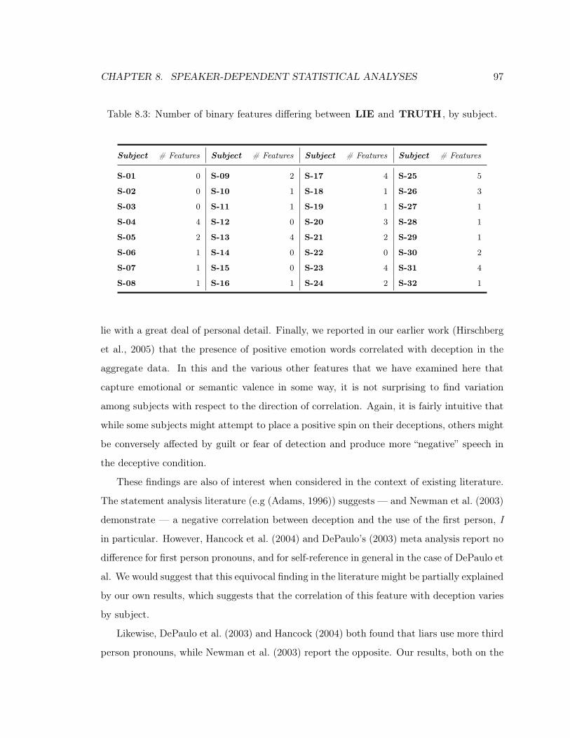
CHAPTER 8. SPEAKER-DEPENDENT STATISTICAL ANALYSES 97
Table 8.3: Number of binary features differing between LIE and TRUTH , by subject.
Subject # Features Subject # Features Subject # Features Subject # Features
S-01 0 S-09 2 S-17 4 S-25 5
S-02 0 S-10 1 S-18 1 S-26 3
S-03 0 S-11 1 S-19 1 S-27 1
S-04 4 S-12 0 S-20 3 S-28 1
S-05 2 S-13 4 S-21 2 S-29 1
S-06 1 S-14 0 S-22 0 S-30 2
S-07 1 S-15 0 S-23 4 S-31 4
S-08 1 S-16 1 S-24 2 S-32 1
lie with a great deal of personal detail. Finally, we reported in our earlier work (Hirschberg
et al., 2005) that the presence of positive emotion words correlated with deception in the
aggregate data. In this and the various other features that we have examined here that
capture emotional or semantic valence in some way, it is not surprising to find variation
among subjects with respect to the direction of correlation. Again, it is fairly intuitive that
while some subjects might attempt to place a positive spin on their deceptions, others might
be conversely affected by guilt or fear of detection and produce more “negative” speech in
the deceptive condition.
These findings are also of interest when considered in the context of existing literature.
The statement analysis literature (e.g (Adams, 1996)) suggests — and Newman et al. (2003)
demonstrate — a negative correlation between deception and the use of the first person, I
in particular. However, Hancock et al. (2004) and DePaulo’s (2003) meta analysis report no
difference for first person pronouns, and for self-reference in general in the case of DePaulo et
al. We would suggest that this equivocal finding in the literature might be partially explained
by our own results, which suggests that the correlation of this feature with deception varies
by subject.
Likewise, DePaulo et al. (2003) and Hancock (2004) both found that liars use more third
person pronouns, while Newman et al. (2003) report the opposite. Our results, both on the
CHAPTER 8. SPEAKER-DEPENDENT STATISTICAL ANALYSES 98
one subject for whom this feature is significant on a by-subject basis, and in the corpus
overall (see Table 4.2), are in accord with the former: we find a positive correlation with
deception and third-person pronouns.
Burgoon et al. (2003) found a greater incidence of both negative and positive emotion
words in deceptive speech; Newman et al. (2003) report a higher incidence of negative
emotion words. We again find our data evenly split among subjects in this regard; on the
corpus overall, we show a positive correlation between the use of positive emotion words and
deception (again, see Table 4.2, on page 38).
The features hasNot, hasNaposT and hasNo capture the concept referred to in the lit-
erature as negation, and here, too, while our overall corpus shows a positive correlation
between the incidence of hasNot and hasNaposT and deception, our results are split in the
by-subject analysis. In the literature, Adams et al. (2006) and DePaulo et al. (2003) report a
positive correlation between deception and negation, while Hancock (2004) finds no effect.
There is no shortage of inconsistent and negative findings on individual lexical features
in the deception literature, both across and within studies. A case in point that we have not
cited thus far is the work of Porter and Yuille (1996), who tested 17 lexical and discourse
features — features generally requiring subjective judgements on the part of the listener
that thus have not been examined in our work — taken from four popular deception de-
tection approaches. Their study found that only three of these cues were useful across four
different laboratory deception paradigms. Although we have not yet tied our findings to
specific personality traits, we suggest that by painting an interesting picture of the variation
across subjects with respect to deceptive speaking styles, our results on lexical features help
to explain the somewhat inconsistent findings that pervade the deception literature: many
features seem to be salient across multiple subjects, but individuals’ behaviors are idiosyn-
cratic with respect to the direction of correlation of those features with deception. We shall
explore this phenomenon with respect to our numerical features in the section that follows.

CHAPTER 8. SPEAKER-DEPENDENT STATISTICAL ANALYSES 99
8.3 Results on Numeric Features
We concern ourselves in the present section with a within-subject analysis of numerical
features that represent a subset of our broader feature set. In particular, we examine those
features to which no normalization scheme has been applied, since our interest is to examine
differences between the TRUTH and LIE conditions within individual subjects. Table 8.4
provides a complete list of the features examined, and the numerical indices provide a key
for the tabular presentation of our detailed results below.
These non-normalized features are representative of the broader feature set, and include
a number of lexical, discourse, and paralinguistic features that are represented numerically
(e.g. laughs, filled pauses, repeated words); pause related features; durational features;
phone counts; energy features, capturing in particular prosodic aspects of energy that are
operationalized as energy slopes; and a large number of F0 and pitch related prosodic fea-
tures, both raw and stylized.
The approach taken here, that is, to apply two statistical tests (the Mann-Whitney U
test and the Kolmogorov-Smirnov test) to each of 88 numeric features for each subject,
represents an enormous number of potential statistical results — 88× 32× 2 = 2, 816 — to
examine, so we ask the readers’ indulgence as we introduce our approach to considering this
data.
As with binary features, there are three broad classes of phenomena that are of interest
here: the frequency with which a given feature is significant across subjects; the frequency
with which a given subject demonstrates significant differences between the TRUTH and
LIE conditions across the features, and the degree to which various subjects exhibit similar
behaviors in the TRUTH and LIE conditions. Because the numerical data represented
here does not suffer from the issue of sparsity encountered in the binary data, we obtained
many significant results at the 0.01 level, and we will consider primarily these results when
addressing the question of similar behaviors among subjects. In the interest of thoroughness,
we present our initial findings at both the 0.05 and 0.01 levels; these are reported in separate
diagrams and tables in order to simplify presentation.
An examination of the results here again supports the view that individuals exhibit great
variation with regard to cues to deceptive speech, both in terms of the number of significant

CHAPTER 8. SPEAKER-DEPENDENT STATISTICAL ANALYSES 100
Table 8.4: Key to numeric features analyzed in Chapter 8.
# Feature # Feature
1 numFilledPause 45 F0_RAW_LAST
2 complexity 46 F0_STY_MAX
3 repeatedWordCount 47 F0_STY_MEAN
4 NUM_WORDS.UNIT_LENGTH.R 48 F0_STY_MIN
5 laugh_TCOUNT 49 F0_STY_FIRST
6 breath_TCOUNT 50 F0_STY_LAST
7 speaker_noise_TCOUNT 51 F0_NUM_D_FRAMES
8 dash_slash_TCOUNT 52 F0_NUM_F_FRAMES
9 slash_TCOUNT 53 F0_NUM_H_FRAMES
10 mispronounced_word_TCOUNT 54 F0_NUM_R_FRAMES
11 unintelligible_TCOUNT 55 F0_NUM_V_FRAMES
12 PREV_PAUSE 56 F0_NUM_D_FRAMES.UNIT_LENGTH.R
13 NEXT_PAUSE 57 F0_NUM_F_FRAMES.UNIT_LENGTH.R
14 TOTAL_PAUSE 58 F0_NUM_H_FRAMES.UNIT_LENGTH.R
15 MAX_PAUSE 59 F0_NUM_R_FRAMES.UNIT_LENGTH.R
16 PAUSE_COUNT 60 F0_NUM_V_FRAMES.UNIT_LENGTH.R
17 TOTAL_PAUSE.UNIT_LENGTH.R 61 F0_NUM_D_FRAMES.F0_NUM_V_FRAMES.R
18 DUR_PHONE_NON_MAX 62 F0_NUM_F_FRAMES.F0_NUM_V_FRAMES.R
19 DUR_PHONE_NON_AV 63 F0_NUM_H_FRAMES.F0_NUM_V_FRAMES.R
20 DUR_PHONE_IN_LIST_NON_MAX 64 F0_NUM_R_FRAMES.F0_NUM_V_FRAMES.R
21 DUR_PHONE_IN_LIST_NON_AV 65 F0_STY_MAX.F0_STY_MIN.D
22 DUR_PHONE_IN_LIST_NON_FIRST 66 F0_RAW_MAX.F0_RAW_MIN.D
23 DUR_PHONE_IN_LIST_NON_LAST 67 F0_MEDFILT_MAX.F0_MEDFILT_MIN.D
24 PHONE_COUNT 68 F0_SLOPES_FIRST
25 PHONE_IN_LIST_COUNT 69 F0_SLOPES_LAST
26 PHONE_COUNT.UNIT_LENGTH.R 70 F0_SLOPES_LENGTH_FIRST
27 PHONE_IN_LIST_COUNT.UNIT_LENGTH.R 71 F0_SLOPES_LENGTH_LAST
28 EG_NO_UV_NUM_F_FRAMES 72 F0_SLOPES_LENGTH_FIRST.UNIT_LENGTH.R
29 EG_NO_UV_NUM_R_FRAMES 73 F0_SLOPES_LENGTH_LAST.UNIT_LENGTH.R
30 EG_NO_UV_NUM_F_FRAMES.UNIT_LENGTH.R 74 F0_SLOPES_MAX_NEG
31 EG_NO_UV_NUM_R_FRAMES.UNIT_LENGTH.R 75 F0_SLOPES_MAX_POS
32 EG_NO_UV_SLOPES_FIRST 76 F0_SLOPES_AVERAGE
33 EG_NO_UV_SLOPES_LAST 77 F0_SLOPES_NOHD_FIRST
34 EG_NO_UV_SLOPES_MAX_NEG 78 F0_SLOPES_NOHD_LAST
35 EG_NO_UV_SLOPES_MAX_POS 79 F0_SLOPES_NOHD_LENGTH_FIRST
36 EG_NO_UV_SLOPES_AVERAGE 80 F0_SLOPES_NOHD_LENGTH_LAST
37 EG_NO_UV_SLOPES_NUM_CHANGES 81 F0_SLOPES_NOHD_LENGTH_FIRST.UNIT_LENGTH.R
38 EG_NO_UV_SLOPES_NUM_CHANGES.UNIT_LENGTH.R 82 F0_SLOPES_NOHD_LENGTH_LAST.UNIT_LENGTH.R
39 EG_NO_UV_STY_MAX.EG_NO_UV_STY_MIN.D 83 F0_SLOPES_NOHD_MAX_NEG
40 EG_NO_UV_RAW_MAX.EG_NO_UV_RAW_MIN.D 84 F0_SLOPES_NOHD_MAX_POS
41 F0_RAW_MAX 85 F0_SLOPES_NOHD_AVERAGE
42 F0_RAW_MEAN 86 F0_SLOPES_NOHD_NUM_CHANGES
43 F0_RAW_MIN 87 F0_SLOPES_NOHD_NUM_CHANGES.UNIT_LENGTH.R
44 F0_RAW_FIRST 88 F0_SLOPES_NOHD_NUM_CHANGES.F0_NUM_V_FRAMES.R

CHAPTER 8. SPEAKER-DEPENDENT STATISTICAL ANALYSES 101
Figure 8.1: Counts of significant numerical features by subject at the 0.01 significance level.
cues, which cues are significant, and the directions of those cues’ correlations with deception.
Figure 8.1 indicates that the number of features that show significance for at least one test
(the Mann-Whitney U test or the Kolmogorov-Smirnov test) at the 0.01 level for
any given subject range from 0 (four subjects) to 20 (one subject), with mean 4.13, std. dev.
5.43, mode 1 and median 2. Figure 8.2 indicates the same counts at the 0.05 level, ranging
from 1 (two subjects) to 37 (one subject), with mean 10.91, std. dev. 10.13, mode 4 and
median 7.5. Figure 8.3 displays the number of subjects with significant variation for the
given feature (on at least one test) at the 0.01 level, ranging from 0 (17 features) to 6 (one
feature), with mean 1.25, std. dev. 1.31, mode 1 and median 1. At the 0.05 level (Figure
8.4), we find only three features that vary significantly for zero subjects, and one feature
varying significantly for ten subjects, with mean 3.84, std. dev. 2.37, mode 3 and median
3. A two-tailed t-test revealed no significant difference between genders with respect to the
number of significant features.

CHAPTER 8. SPEAKER-DEPENDENT STATISTICAL ANALYSES 102
Figure 8.2: Counts of significant numerical features by subject at the 0.05 significance level.

CH
AP
TE
R8.
SP
EA
KE
R-D
EP
EN
DE
NT
STA
TIS
TIC
AL
AN
ALY
SE
S103
Figure 8.3: Counts of significant numerical features by feature at the 0.01 significance level.
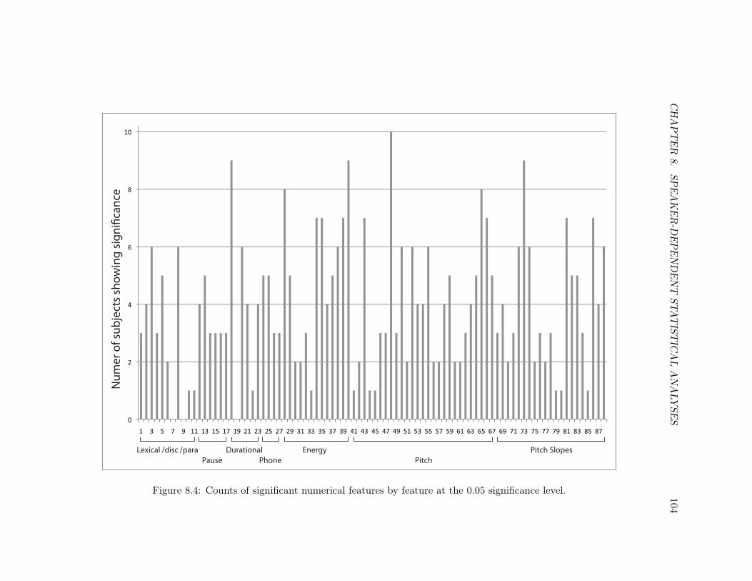
CH
AP
TE
R8.
SP
EA
KE
R-D
EP
EN
DE
NT
STA
TIS
TIC
AL
AN
ALY
SE
S104
Lexical /disc /para
Pause Phone Pitch
Durational Energy Pitch Slopes
Figure 8.4: Counts of significant numerical features by feature at the 0.05 significance level.

CHAPTER 8. SPEAKER-DEPENDENT STATISTICAL ANALYSES 105
Tables 8.5 and 8.6 present the full results by subject and feature for the 0.01 and 0.05 sig-
nificance levels, on pages 106 and 108, respectively.5 These tables illustrate which test(s) are
significant for each subject and feature combination at the given significance level. Reading
horizontally across the table, the reader can determine which of the subjects demonstrated
significant differences between TRUTH and LIE for a given feature; reading vertically
down the table, the reader can determine which features were significant for a given subject;
for both of these tables, indices for features that were not significant for any subject were
omitted in the interest of a more compact presentation (the key to feature indices is found
in Table 8.4 on page 100). As with our binary features, for almost every given feature at
both significance levels there is an even distribution of signs of correlation with deception;
that is, approximately half of the subjects that show significance for a given feature show
positive correlation for deception, while half show negative. As would be expected, these ta-
bles also reveal that in most cases in which the Kolmogorov-Smirnov test is significant,
the Mann-Whitney U test is also significant (indicated with “X” in the table), while in
a number of cases the Mann-Whitney U test— the more sensitive test — is the sole test
that shows significance.
Figures 8.5 and 8.6, on pages 111 and 112 respectively, visualize the relationship among
the counts for the two tests at both significance levels. Figure 8.5 displays counts by subject
and Figure 8.6 displays counts by feature.6 In addition to illustrating the variation across
subjects and features, this table further demonstrates the phenomenon we described whereby
the significant results for the Kolmogorov-Smirnov test generally represent a subset of
those for the Mann-Whitney U test .
5These many results are presented in their entirety for the sake of completeness. Later in this chapter
we offer more human-readable presentations of these results; therefore the reader is encouraged only to skim
these tables at this time and to refer back to the details only as need or interest may dictate.
6These figures differ from the previous graphs of counts in that they represent each test individually. In
the the bar graphs of Figures 8.1 through 8.4 each instance counted refers to the event that either or both
tests were significant for a given feature and subject; the total counts thus differ because the earlier figures
represent the counts (where significant) | MW ∪ KS \ (MW ∩ KS) | for each feature or subject.

CH
AP
TE
R8.
SP
EA
KE
R-D
EP
EN
DE
NT
STA
TIS
TIC
AL
AN
ALY
SE
S106
Table 8.5: Significance of Mann-Whitney, Kolmogorov-Smirnov, or both tests (X), with sign of correlation with LIE , at 0.01 level.
Sub⇒ 1 2 3 4 5 6 7 8 9 10 11 12 13 14 15 16 17 18 19 20 21 22 23 24 25 26 27 28 29 30 31 32
1 - - - - - - - - - - - - M+ - - - - - - - - - - - - - - - - - - -2 - - - - - - - - - - - - - - - - - - - - - - - M- - - - - - - - -3 - - - - - - - M+ - - - - - - M- - M- - - - - - - - - - - - - - - -4 - - - - - - - - - - - - - - - - - - - X- - - - - - - - - - - - -5 - - M+ - - - - M+ - - - - - - - - - - - - - - - - - M+ - - - - - -6 - - - - - - - - - - - - - - - - - - M- - - - - - - - - - - - - -8 - - - - - - - - - - M- - - - - - - - - - - - - - - - - - - - - -
11 - - - - - - - M+ - - - - - - - - - - - - - - - - - - - - - - - -13 - - - - X+ - - - - - - - - - - - - - - - - - - - - - - - - - - -14 - - - - X- - - - - - - - M+ - - - - - - - - - - - - - - - - - - -15 - - - - X- - - - - - - - - - - - - - - - - - - - - - - - - - - -16 - - - - X- - - - - - - - - - - - - - - - - - - - - - - - - - - -17 - - - - X- - - - - - - - - - - - - - - - - - - - - - - - - - - -18 - - - - - - K- M+ K- - - - - - - - - - - - - - - - - - - - - - - -20 - - - - X- - - - - - - - - - - - - - - - - - - - X+ - - - - M+ - -21 - - - - X- - - - - - - - - - - - - - - - - - - - - - - - - M+ - -22 - - - - - - - - - - - - - - - - - - - - - - - - - - M+ - - - - -23 - - - - M- - - - - - - - - - - - - - - - - - - - - - - X- - - - -24 - - - - M- - - - - - - - M+ - - - - - - - - - - - M+ - - - - - - K-25 - - - - M- - - - - - - - - - - - - - - M- - - - - M+ - - - - - - K-28 - - - - M- - - - - - - - X+ - - - - - - M- - - - - M+ - - - - - - -29 - - - - X- - - - - - - - - - - - - - - M- - - - - M+ - - - - M+ - -34 - - - - - - - X- - - - - M- - - - - - - - - - - - - - - - - - - -35 - - - - - - - - - - - - - - - K+ - - - - - - M- - - X- - - - X+ - -36 - - - - - - - - - - - - M- - - - - - - - - - - - - - M- - - - - -37 - - - - M- - - - - - - - M+ - - - - - - - - - - - M+ - - - - - - -38 - - - - X+ X- - M- - - - - - - - - - - - - - - - - - - - - - - - -39 - - - - - - - X+ - - - - X+ - - - X- - - X- - - - - - - - - - X+ - -40 - - - - - - - X+ - - - - X+ - - - M- - - K- - - M- - - - - - - X+ - -41 - - - - - - K+ - - - - - - - - - - - - - - - - - - - - - - - - -42 - - - - - - - - - - M+ - - - - - - - - - - - - - - - - - - - - -43 - - - - - - - - - - - - - - - - - - - X+ - - - - - - - - - - K+ -45 - - - - - - - - - - - - - - - - - - - - - - - - - - M- - - - - -47 - - - - - - - - - - M+ - - - - - - - - - - - - - - - - - - - - -48 - - - - - - - - - - - - - - - - - - - M+ - - - - - - - - - - - -
Continued . . .

CH
AP
TE
R8.
SP
EA
KE
R-D
EP
EN
DE
NT
STA
TIS
TIC
AL
AN
ALY
SE
S107
Table 8.5 — Continued
Sub⇒ 1 2 3 4 5 6 7 8 9 10 11 12 13 14 15 16 17 18 19 20 21 22 23 24 25 26 27 28 29 30 31 32
49 - - - - - - - - - - - - - - - - - - - - - - - - - - - - - K- - -50 - - - - - - - - - - - - - - - - - - - - - - - - - - M- - - - - -51 - - - - - - - - - - - - - - - - - - - - - - - - - - - - - - M+ -52 - - - - M- - - - - - - - M+ - - - - - - M- - - - - - - - - - M+ - -53 - - - - - - - - - - - - - - - - - - - - - - - - X+ - - - - - - -54 - - - - X- - - - - - - - - - - - - - - - - - - - M+ - - - - - - -55 - - - - M- - - - - - - - X+ - - - - - - M- - - - - M+ - - - - - - -56 - - - - - - - - - - - - - - - - - - - - - - - - - - - - - - M+ -57 - - - - - - - - - - - - - - - - - - - X- - - - - - - - - - - - -58 - - - - - - - - - - - - - - - - - - - - - X+ - - X+ - - - - - - -59 - - - - - - - - K+ M+ - - - - - - - - - - - - - - - - - - - - - -60 - - - - - - - - - - - - - - - - - - - X- - - - - - - - - - - - -61 - - - - - - - - - - - - - - - - - - - - - - - - - - - - - - M+ -62 - - - - - - - - - - - - - - - - - - - K- - - - - - - - - - - - -63 - - - - - - - - - - - - - - - - - - - - - K+ - - X+ - - - - - - -64 - - - - - - - - - - - - - - - - - - - K+ - - - - - - - - - - - -65 - - - - - - - M+ - - - - - - - - M- - - X- - - - - - - - - - - - -66 - - - - - - - - - - - - - - - - - - - X- - - - - - - - - - - - -67 - - - - - - - - - - - - - - - - - - - X- - - - - - - - - - - - -68 - - - - - - - - - - - - - - - - - M+ - - - - - - - - - - - - - -69 - - - - - - - - - - - - - K- - - - - - - - - - - - - - - - - - -70 - - - - - - - - - - - - - - - - - - - - M+ - - - - - - - - - - -72 - - - - - - - - - - - - - - - - - - - - M+ - - - M- - - - - - - -73 - - - - - - - M- - - - - - - - - - - - - - - - - - - - - - - - -74 - - - - - - - - - - - - - - - - - - - X+ - - - - - - - - - - - -75 - - - - - - - - - - - - - - - - - - - - - - - - X+ M- - - - - - -76 - - - - - - - - - - - - - M- - - - - - - - - - - - - - - - - - -77 - - - - - - - - - - - - - - - - - M+ - - - - - - - - - - - - - -78 - - - - - - - - - - - - - K- - - - - - - - - - - - - - - - - - -79 - - - - - - - - - - - - - - - - - - - - M+ - - - - - - - - - - -81 - - - - - - - - - - - - - - - - - - - - X+ - - - M- - - - - - - -83 - - - - - - - - - - - - - - - - - - - X+ - - - - - - - - - - - -84 - - - - - - - - - - - - - - - - - - - - - - - - X+ M- - - - - - -86 - - - - X- - - - - - - - M+ - - - - - - - - - - - M+ - - - - - - -87 - - - - M+ - - - - - - - - - - - - - - - - - - M+ - - - - - - - -88 - - - - - - - - - - - - - - - - - - - K+ - - - - - - - - - - - -

CH
AP
TE
R8.
SP
EA
KE
R-D
EP
EN
DE
NT
STA
TIS
TIC
AL
AN
ALY
SE
S108
Table 8.6: Significance of Mann-Whitney, Kolmogorov-Smirnov, or both tests (X), with sign of correlation with LIE , at 0.05 level.
Sub⇒ 1 2 3 4 5 6 7 8 9 10 11 12 13 14 15 16 17 18 19 20 21 22 23 24 25 26 27 28 29 30 31 32
1 - - - - - - - - - - - - X+ - - - - - - - M- - - - M- - - - - - - -2 - - M- M- - - - - - - - - - - - - - - - - M- - - X- - - - - - - - -3 - - - - - - - X+ M- - - - - - M- - X- - - - - - - - M+ M- - - - - - -4 - - - - K+ - - - - - - - - - - - - - - X- - - - M+ - - - - - - - -5 - - M+ - - M+ - M+ - - - - - - - - - - - - - - - - - M+ - - - M+ - -6 - - - - M+ - - - - - - - - - - - - - M- - - - - - - - - - - - - -8 - - - - - - - - - - M- - - M+ - - - - - M- - - - - M+ - - M+ - M+ - -
10 - - - - - - - - - - - - - - - - M- - - - - - - - - - - - - - - -11 - - - - - - - M+ - - - - - - - - - - - - - - - - - - - - - - - -12 - - - - X+ - - - - - - - - - - - - - M- X+ - - - - - - - M+ - - - -13 - - M+ - X+ - - X+ - - - - - - - - - - - K+ - M+ - - - - - - - - - -14 - - - - X- M+ - - - - - - X+ - - - - - - - - - - - - - - - - - - -15 - - - - X- M+ - - - - - - X+ - - - - - - - - - - - - - - - - - - -16 - - - - X- M+ - - - - - - M+ - - - - - - - - - - - - - - - - - - -17 - - - - X- M+ - - - - - - M+ - - - - - - - - - - - - - - - - - - -18 M- - - - M- X+ X- X+ X- - - - X+ - - - - - - - X- - - - - - - - - M+ - -20 - - - - X- - - M+ - - - - - - - - - - - - M- - - - X+ - - M- - X+ - -21 - - - - X- - - - - - - - M- - K+ - - - - - - - - - - - - - - X+ - -22 - - - - - - - - - - - - - - - - - - - - - - - - - - M+ - - - - -23 - - - - X- - - - - - - - - - - - - - - - M- - - - X+ - - X- - - - -24 - - - - X- - - - - - - - M+ - - - - - - X- - - - - X+ - - - - - - X-25 - - - - M- - - - - - - - M+ - - - - - - X- - - - - X+ - - - - - - X-26 M+ - - - M+ - - - - - - - - - - - - - - - - - - - - - - - - M- - -27 M+ - - - M+ - - M- - - - - - - - - - - - - - - - - - - - - - - - -28 - - - - X- - - - - - - - X+ - - K+ - - - M- - - - M- X+ - - - - M+ - M-29 - - - - X- - - - - - - - X+ - - - - - - X- - - - - X+ - - - - X+ - -30 - - - - - - - - - - - - - - - - - - M- M- - - - - - - - - - - - -31 X- - - - - - - - - - - - - - - - - - - - - - - - - - - - - M+ - -32 - - - K+ - - - M+ - - - - - - - - - - - - - - - X- - - - - - - - -33 - - - - - - - K- - - - - - - - - - - - - - - - - - - - - - - - -34 - - - - M+ - - X- - - - - X- - - - K+ M- - - - - - - X- - - - - X- - -35 - - - - - - - X+ - - - - X+ - - X+ - - - - - - X- - M+ X- - - - X+ - -36 - - - - - - - M- - - - - X- M+ - - - - - - - - - - - - X- - - - - -37 - - - - X- - - - - - - - X+ - - - - - - X- - - - - M+ - - - - - - M-38 - - - - X+ X- - M- - - - - - - - - - - - - M+ - - M+ - - M+ - - - - -
Continued . . .
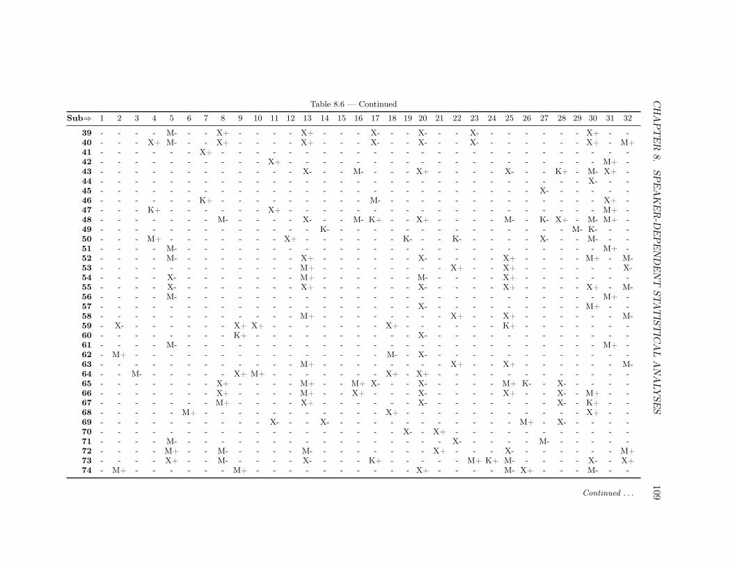
CH
AP
TE
R8.
SP
EA
KE
R-D
EP
EN
DE
NT
STA
TIS
TIC
AL
AN
ALY
SE
S109
Table 8.6 — Continued
Sub⇒ 1 2 3 4 5 6 7 8 9 10 11 12 13 14 15 16 17 18 19 20 21 22 23 24 25 26 27 28 29 30 31 32
39 - - - - M- - - X+ - - - - X+ - - - X- - - X- - - X- - - - - - - X+ - -40 - - - X+ M- - - X+ - - - - X+ - - - X- - - X- - - X- - - - - - - X+ - M+41 - - - - - - X+ - - - - - - - - - - - - - - - - - - - - - - - - -42 - - - - - - - - - - X+ - - - - - - - - - - - - - - - - - - - M+ -43 - - - - - - - - - - - - X- - - M- - - - X+ - - - - X- - - K+ - M- X+ -44 - - - - - - - - - - - - - - - - - - - - - - - - - - - - - X- - -45 - - - - - - - - - - - - - - - - - - - - - - - - - - X- - - - - -46 - - - - - - K+ - - - - - - - - - M- - - - - - - - - - - - - - X+ -47 - - - K+ - - - - - - X+ - - - - - - - - - - - - - - - - - - - M+ -48 - - - - - - - M- - - - - X- - - M- K+ - - X+ - - - - M- - K- X+ - M- M+ -49 - - - - - - - - - - - - - K- - - - - - - - - - - - - - - M- K- - -50 - - - M+ - - - - - - - X+ - - - - - - K- - - K- - - - - X- - - M- - -51 - - - - M- - - - - - - - - - - - - - - - - - - - - - - - - - M+ -52 - - - - M- - - - - - - - X+ - - - - - - X- - - - - X+ - - - - M+ - M-53 - - - - - - - - - - - - M+ - - - - - - - - X+ - - X+ - - - - - - X-54 - - - - X- - - - - - - - M+ - - - - - - M- - - - - X+ - - - - - - -55 - - - - X- - - - - - - - X+ - - - - - - X- - - - - X+ - - - - X+ - M-56 - - - - M- - - - - - - - - - - - - - - - - - - - - - - - - - M+ -57 - - - - - - - - - - - - - - - - - - - X- - - - - - - - - - M+ - -58 - - - - - - - - - - - - M+ - - - - - - - - X+ - - X+ - - - - - - M-59 - X- - - - - - - X+ X+ - - - - - - - X+ - - - - - - K+ - - - - - - -60 - - - - - - - - K+ - - - - - - - - - - X- - - - - - - - - - - - -61 - - - - M- - - - - - - - - - - - - - - - - - - - - - - - - - M+ -62 - M+ - - - - - - - - - - - - - - - M- - X- - - - - - - - - - - - -63 - - - - - - - - - - - - M+ - - - - - - - - X+ - - X+ - - - - - - M-64 - - M- - - - - - X+ M+ - - - - - - - X+ - X+ - - - - - - - - - - - -65 - - - - - - - X+ - - - - M+ - - M+ X- - - X- - - - - M+ K- - X- - - - -66 - - - - - - - X+ - - - - M+ - - X+ - - - X- - - - - X+ - - X- - M+ - -67 - - - - - - - M+ - - - - X+ - - - - - - X- - - - - - - - X- - K+ - -68 - - - - - M+ - - - - - - - - - - - X+ - - - - - - - - - - - X+ - -69 - - - - - - - - - - X- - - X- - - - - - - - - - - - M+ - X- - - - -70 - - - - - - - - - - - - - - - - - - X- - X+ - - - - - - - - - - -71 - - - - M- - - - - - - - - - - - - - - - - X- - - - - M- - - - - -72 - - - - M+ - - M- - - - - M- - - - - - - - X+ - - - X- - - - - - - M+73 - - - - X+ - - M- - - - - X- - - - K+ - - - - - M+ K+ M- - - - - X- - X+74 - M+ - - - - - - M+ - - - - - - - - - - X+ - - - - M- X+ - - - M- - -
Continued . . .

CH
AP
TE
R8.
SP
EA
KE
R-D
EP
EN
DE
NT
STA
TIS
TIC
AL
AN
ALY
SE
S110
Table 8.6 — Continued
Sub⇒ 1 2 3 4 5 6 7 8 9 10 11 12 13 14 15 16 17 18 19 20 21 22 23 24 25 26 27 28 29 30 31 32
75 - - - - - - - - - - - - - - - - - - - - - - - - X+ X- - - - - - -76 - - - - - - - - - M+ - - - X- - - - M+ - - - - - - - - - - - - - -77 - - - - - M+ - - - - - - - - - - - X+ - - - - - - - - - - - - - -78 - - - - - - - - - - - - - X- - - - - - - - - - - - M+ - X- - - - -79 - - - - - - - - - - - - - - - - - - - - X+ - - - - - - - - - - -80 - - - - - - - - - - - - - - - - - - - - - - - - - - M- - - - - -81 - - - - X+ - - M- - - - - M- - - - - - - - X+ - - M+ X- - - - - - - M+82 - - - - M+ - - X- - - - - X- - - - - - - - - - M+ - - - - - - X- - -83 - M+ - - - - - - - - - - - - - - - - - X+ - - - - M- X+ - - - X- - -84 - - - - - - - - - - - - - - - - M- - - - - - - - X+ X- - - - - - -85 - - - - - - - - - - - - - - - - - M+ - - - - - - - - - - - - - -86 - - - - X- - - K+ - - - - M+ - - M+ - - - X- - - - - X+ - - - - - - M-87 - - - - X+ M- - - - - - - - - - - - - - - - - - X+ - - M+ - - - - -88 - - - - X+ M- - - - - - - - - - - - - - X+ - - - K+ - - M+ - - M- - -

CH
AP
TE
R8.
SP
EA
KE
R-D
EP
EN
DE
NT
STA
TIS
TIC
AL
AN
ALY
SE
S111
!"
#"
$!"
$#"
%!"
%#"
&!"
&#"
'!"
($" (%" (&" ('" (#" ()" (*" (+" (," ($!"($$"($%"($&"($'"($#"($)"($*"($+"($,"(%!"(%$"(%%"(%&"(%'"(%#"(%)"(%*"(%+"(%,"(&!"(&$"(&%"
-."/01!$"
2("/01!$"
-."/01!#"
2("/01!#"
Figure 8.5: Counts of significant numerical features by test and subject.

CH
AP
TE
R8.
SP
EA
KE
R-D
EP
EN
DE
NT
STA
TIS
TIC
AL
AN
ALY
SE
S112
!"
#"
$"
%"
&"
'"
("
)"
*"
+"
#!"
#" %" '" )" +" ##"#%"#'"#)"#+"$#"$%"$'"$)"$+"%#"%%"%'"%)"%+"&#"&%"&'"&)"&+"'#"'%"''"')"'+"(#"(%"('"()"(+")#")%")'"))")+"*#"*%"*'"*)"
,-"./0!#"
12"./0!#"
,-"./0!'"
12"./0!'"
Figure 8.6: Counts of significant numerical features by test and feature.

CHAPTER 8. SPEAKER-DEPENDENT STATISTICAL ANALYSES 113
8.3.1 Discussion of feature classes
Figures 8.7 and 8.8 (on pages 114 and 115) provide the basis for a more high-level discussion
of our results. These figures depict the grid of subject-by-feature results at the 0.01 signifi-
cance level overlaid with a key to the categories of those features. The majority of cues that
showed significance for multiple subjects come from the classes of energy and pitch features,
but there are a few notable exceptions.
Among lexical, discourse, and paralinguistic features, we find two that were significant
for a number of subjects: repeatedWordCount (#3) and the count of laughs (#5). The
former showed correlations in both directions, but the latter is notable in that it is one
of the few features in these analyses to show itself to be correlated in the same direction
(positive) with deception for all subjects, albeit only three.
There is a limited attention paid in the literature to repetition in speech as a deception
cue. DePaulo, et al. (2003) examined this cue as part of the “fluency” component of their
theoretical construct that addresses the degree to which liars are less compelling than truth
tellers. Their meta-analysis found that repetitions are significantly and positively correlated
with deception across four studies. Vrij (2008) considered repetitions under the broader
rubric of “speech errors” and found such errors to be inconclusive across 44 studies that
examined them. Among those studies, twenty observed some significant correlation between
speech errors and deception, with the majority of those (17) showing a positive correlation.
The literature likewise pays surprisingly little express attention to laughter, as separate
from smiling, as a cue to deception. We were unable to find specific reference to laughter
as a cue, even in DePaulo, et al’s (2003) and Vrij’s (2008) exhaustive reviews; Ekman’s
(2001) influential book likewise addresses only smiling as a cue. Both Vrij and DePaulo et
al. examined smiling (the latter treating smiling as a component of the broader construct
examining pleasantness), and reported insignificant findings over the many studies they
considered. Of the studies Vrij examined that did show significance, there was again a
conflict in the direction of correlation with deception. Ekman (2001) is of help here, since
he considers the smile in context – that is, he suggests that smiling is a cue to deception
when it is inconsistent with the emotion or mood that is overtly portrayed by the speaker.
We would claim that laughter is in some ways analogous to smiling, and that our results are

CH
AP
TE
R8.
SP
EA
KE
R-D
EP
EN
DE
NT
STA
TIS
TIC
AL
AN
ALY
SE
S114
Figure 8.7: Numerical features significant at the 0.01 level, showing feature categories (continues next page).

CH
AP
TE
R8.
SP
EA
KE
R-D
EP
EN
DE
NT
STA
TIS
TIC
AL
AN
ALY
SE
S115Figure 8.8: Numerical features significant at the 0.01 level, showing feature categories, continued.

CHAPTER 8. SPEAKER-DEPENDENT STATISTICAL ANALYSES 116
again consistent with the literature insofar as they vary across subjects (possibly explaining
the inconclusive results of aggregate studies) and also in that Ekman’s theory potentially
explains these conflicting behaviors.
No particular pause feature is of real note (though the total duration of all pauses in the
segment was significant for two subjects, albeit in different directions); however, one subject
showed significance on both tests for all five pause features, with negative correlations with
deception for the features capturing pauses in the current segment and positive correlation
for the length of the preceding pause. The literature is again ambiguous with regard to
the significance of pausing as a cue: Mann et al. (2002) found in real, high-stakes police
interviews that deceivers produced more total internal pauses. On the other hand, Bond
et al. (1990) found no effect for deception on silent pauses in a study of both American
and Jordanian subjects. Anolli and Ciceri (1997) found an increased number of pauses in
deception in Italian speakers. Vrij (2008) found that liars exhibited increased pause dura-
tion across multiple studies — in this instance, the studies that showed a significant effect
(5/12) on pausing were unanimous in finding a positive correlation with deception; a similar
examination of pause frequency was inconclusive. DePaulo found no effect with regard to
silent pauses across 26 studies, which they examined under the “fluency” component of their
broader construct capturing the degree to which speakers are compelling. We hesitate to
offer strong interpretations here given our finding that the pause features were significant for
essentially one subject, but again, we find it interesting that this one subject demonstrated
significance five of six possible features.
Significant durational features are likewise sparse, with a few exceptions. Average and
maximum phone duration for a segment (features #18 and #19) each demonstrate signif-
icance for three subjects, again with varying directions of correlation. The literature on
phone durations is also sparse, with the notable exception of Hall’s (1986) Ph.D. thesis,
which examined syllabic duration of (one word) Control Question Test polygraph responses,
and found increased duration in deceptive answers.
Two phone-count features are significant for four subjects each (with overlap in three
cases). These features (#24 and #25), which count overall phones and phones representing
SAE vowels, respectively, do not appear to our knowledge in the deception literature. They

CHAPTER 8. SPEAKER-DEPENDENT STATISTICAL ANALYSES 117
capture, in the abstract, phonological variety in the utterances, but we hesitate to speculate
as to the importance of this concept in deceptive speech.
A number of energy features are of interest, and in general at least one energy feature
showed significance in twelve subjects. In particular, features #28 and #29, which capture
the number of falling or rising frames (with regard to energy) respectively. These features can
be thought of as a measure of energy variation, and this idea gives context to a consideration
of their relationship for three of the subjects (S5, S20, and S25) for which they are significant.
For these three subjects, the correlation with LIE is the same for both features (negative for
S5 and S20 and positive for S25), suggesting that in the LIE condition these speakers flatten
out their speech with respect to energy variation. Features #39 and #40, significant for a
total of six subjects, capture another facet of variability, the difference between minimum and
maximum values. We located one existing study that specifically addressed energy (Motley,
1974), but found no differences between the TRUTH and LIE conditions. A close analog to
our energy features that appears in the deception literature is found in studies that address
amplitude or volume as a cue. Sayenga (Sayenga, 1983) found decreased amplitude in
deceptive passages. In three studies (Hall, 1986; Cestaro & Dollins, 1994; Mehrabian, 1971),
such features did not show significant differences between the TRUTH and LIE conditions,
though in the last named of these three, subjects who were classified as lower in anxiety
exhibited greater average volume. Anolli and Ciceri (1997) likewise found no effect on
amplitude in a study of Italian speakers.
Among studies that examine acoustic cues to deception, pitch has been a popular feature
(e.g. (Streeter et al., 1977; Scherer et al., 1985; Hall, 1986; Ekman et al., 1991)). Italian
speakers have been shown to increase F0 in the LIE condition (Anolli & Ciceri, 1997). In
fact in all the cases of which we are aware, where pitch has been shown to be significant
(in data aggregated over a study’s subjects), pitch is higher in the deceptive condition.
This is true of the studies reported in Vrij’s (2008) meta-analysis, where he found pitch
to be significant across multiple studies, with 6 of 14 individual studies finding significant
differences. Likewise DePaulo et al. (2003) found that pitch was significantly higher in
deception across 23 studies. Scherer et al. (1985) proffer two possible explanations for
this phenomenon. First, they suggest that liars may be more tense and that this might

CHAPTER 8. SPEAKER-DEPENDENT STATISTICAL ANALYSES 118
account for elevated pitch; DePaulo et al. seem to be in agreement, as they include pitch
under their construct that captures the degree to which deceivers are more tense than truth
tellers. Second, Scherer et al. suggest that increased pitch may be part of a self-presentation
strategy that leads the deceiver to speak in a more animated fashion. Results on our own
pitch features seem to support the latter explanation. Although features capturing mean
pitch do not appear to be prominent, several features capturing variation — falling and
rising frames (#52 and #54) and range from minimum to maximum values (#65) — are
significant for a number of subjects. As before, the directions of correlation with deception
vary, and this seems to support Scherer et al’s self-presentational explanation, as well as its
converse, that is, that some speakers may attempt to control (and consequently decrease)
the variation in their speech when lying. One additional feature is of note, that of minimum
stylized pitch (#48). For most of our features, the number of subjects for which they are
significant at the 0.05 level increases in a fairly proportional manner with respect to the
number for which they are significant at the 0.01 level. This particular feature is unusual
in that while it is significant for only one subject at the 0.01 level, it is significant for ten
subjects at the 0.05 level (see Figures 8.3 and 8.3). We point this out since it is the only
feature that varies to this degree at the two significance levels. The relevance of this feature
for such a large number of subjects, albeit at the lower significance level, seems to warrant
further exploration of the magnitude of pitch excursions.
To our knowledge no existing work in the deception literature addresses the features we
class as F0 slope features. A number of these were significant for multiple subjects, again in
several cases confirming that it is variability in pitch that is of interest. In particular, the
number of changes in slope within the segment (#86; three subjects), maximum positive
slope (#84; two subjects) and the ratio of slope changes to unit length (#87; two subjects),
demonstrate this idea.
Also of some interest is the observation that while we count 24 instances of significance of
our pitch slope features across ten subjects, fully 15, or 63%, of these instances are accounted
for by only four subjects (S14, S20, S21, S25). This last observation holds for other feature
classes as well: pitch features show significance for 14 subjects, but 4 (S5, S20, S25, S32)
subjects account for 61% (24/38) of the instances. Energy features are significant for 12

CHAPTER 8. SPEAKER-DEPENDENT STATISTICAL ANALYSES 119
subjects, but 6 of these (S5, S8, S13, S20, S25, S30) account for 76% of the 33 instances.
We also recall to the reader our earlier observation that, while there were only six instances
of significance for our pause features, one subject demonstrated significance on five of the
six possible features. The preceding leads to two additional observations: first, and not
surprisingly, some subjects seem to exhibit multiple effects with respect to related features,
such as multiple pitch features. More interestingly, some subjects seem to overlap or to
share categories. For example, S20 appears in all three of the groups above, as does S25. A
comparison with respect to specific speaking styles is rendered more complicated, however,
by the possibility that the directions of correlation are different for two given subjects on
any one feature. In the next section, we present a novel way of addressing this issue.
8.3.2 Towards a visualization of speaking styles
As we have just observed, a number of speakers show similar behaviors with respect to
significant features, and we were intrigued by the possibility of exploring these similarities
in the interest of inferring particular styles of deceptive speech. In order to do this, we have
conceived of the grid depicted in Figures 8.7 and 8.8 (on pages 114 and 115) as an indirect
adjacency list from which we have constructed the graph shown in Figure 8.97. In this
conception, one reads across the rows of the grid: any cell which indicates a significant test
{K,M,X} represents a potential edge,8 connecting the corresponding subject to any other
subject that has an entry in the same row with the same sign.9. For example, on page 114,
feature #3 (repeatedWordCount) has three entries, at S3 (M+), S15 (M-), and S17 (M-).
This defines an edge between S15 and S17, labeled “3-”, as realized at the left-hand side of
the central cluster of Figure 8.9. Each node of the graph is labeled with its subject number,
7We also generated a graph using the same principle at the 0.05 level of significance, but because of the
enormous number of features significant at this level, the graph was interconnected to the degree that no
coherent clusters were produced, and the visualization created defied interpretation.
8We treat the three cases {K,M,X} as equivalent for the purposes of constructing the graph.
9We considered adding additional edges to this graph for binary features significant at the 0.01 level as
well, but doing so added only seven additional edges, all of which were singletons (i.e. only two subjects
were connected by any given feature and correlation pattern), possibly owing to the sparseness of the data,
and this did not seem to contribute to our goal of inferring generalized speaking styles

CHAPTER 8. SPEAKER-DEPENDENT STATISTICAL ANALYSES 120
Lexical / para
Durational
Phone counts
Energy
Pitch
Pitch Slopes
Cluster A
Cluster B
Figure 8.9: Graph of subjects indicating common significant features, with sign of correlation
with deception; female subjects shaded.

CHAPTER 8. SPEAKER-DEPENDENT STATISTICAL ANALYSES 121
the average detection accuracy achieved on that subject by listeners in the perception study
(see the following chapter and Chapter 10), and the total number of features that registered
significance at the 0.01 level.10
A few observations follow immediately from inspection of the graph we have constructed
from this information. First, the graph contains two large clusters joined by a single edge
between S23 and S26, which we have labeled Cluster A (10 subjects) and Cluster B (8
subjects). There are additionally 10 singleton nodes with degree 0 (ranging in terms of sig-
nificant features from 0 to 4, not shared by any other subject), and one cluster of {S7,S9,S10}
linked by two total edges.
Cluster A is dominated by patterns of features that, with their given directions of cor-
relation, describe speech that is more variable and animated in the deceptive condition.
Energy features are fairly prominent, and in large part correlated positively with deception.
In particular, two features (#39 and #40) that capture range of energy in the segment
appear repeatedly. Other energy features indicating increased or variable energy are also
positively correlated with deception, such as maximum positive slope, (#35), number of
rising frames (#29) and number of slope changes (#37). Maximum negative slope (#34)
appears with negative correlation, but this is in a way consistent with the other features’
behavior, since they capture high or rising energy and this feature captures the opposite.
The average of energy slopes in the segment (#36) is also negatively correlated, but could
be interpreted as indicating variability in the speech. In addition, the count of laughs (#5)
only appears in this cluster, and with positive correlation. Four pitch features appear in this
cluster as well, capturing counts of falling (#52) and voiced (#55) frames, and proportions
of halved frames (#58 and #63), all positively correlated with deception. With only minimal
exceptions, all of the features described here, given their directions of correlation, describe
10This sum differs from the degree of each node in two ways: First, not all features are shared among
multiple subjects, so an arbitrary number of significant features (up to 88) may not be realized as edges;
second, each significant feature is realized by a separate edge connecting a given subject to all other subjects
that demonstrate significance on the same feature with the same direction of correlation, so a subject
demonstrating only one significant feature could still conceivably be represented by a node of any degree
less than 32.

CHAPTER 8. SPEAKER-DEPENDENT STATISTICAL ANALYSES 122
animated speech,11 recalling the possibility broached earlier that some liars “oversell” the lie.
The two measures of pitch halving that appear here do not make an immediately obvious
contribution to this interpretation. However, we recall our earlier observation in Section 4.3
that halving can occur in the presence of vocal fry or diplophonia (Johnson, 2003), that this
might signal “forced” or overly energetic speech production, consistent with the idea that
the speaker is overselling.
The idea of “overselling” is perhaps related to the factors DePaulo et al. (2003) label
“engaging” and “immediate” as part of their overall construct capturing the degree to which
liars are less compelling than truth tellers. The features prominent in this cluster — laughter,
increased energy, increased pitch variability, all suggest speech that is more, and perhaps
intentionally, engaging in the LIE condition. In this sense, our observations suggest a
contrast to the hypothesis of DePaulo, since we find deceptive speech to be potentially more
engaging, at least with respect to the two factors termed “engaging” and “immediate”.
Cluster B is conversely dominated by features (and their respective directions of corre-
lation) that suggest less animated speech in the deceptive condition. Notably, the energy
features (#39 and #40) that capture range of energy in the segment appear repeatedly and
with negative correlation, in contrast with Cluster A. Energy features that capture max-
imum positive slope (#35) and rising frames (#29) are also negatively correlated. Pitch
features are also consistent with less animation or vocal immediacy: minimum pitch (#43)
is positively correlated with deception, while falling frames (#52) and voiced frames (#55)
are negatively correlated, as is a feature capturing vowel duration (#23). Repeated word
count (#3) is negatively correlated for two speakers, and this could be interpreted as re-
flecting more careful speech, consistent with a lack of animation. One exception to our
interpretation is the measure of density of pitch slope changes (#87), which is positively
correlated with deception in this cluster. Overall, however, the subjects in Cluster B seem to
behave consistently with DePaulo’s hypothesis with respect to speakers’ being less engaging
and immediate in deception. Taken together with our observations on Cluster A, our find-
ings here are again consistent with our repeated claim that deceptive behaviors vary across
subjects with respect to the same types of cues, in this case that the speakers of Cluster A
11One feature, capturing changes in slope (#38), is a clear exception for the two subjects it links.

CHAPTER 8. SPEAKER-DEPENDENT STATISTICAL ANALYSES 123
are more engaging in deception, while the speakers of Cluster B are less so.
8.4 Conclusions
We have presented in this chapter considerable evidence to suggest that, while many speak-
ers share certain salient cues in deception, the manifestation of those cues (represented here
in terms of their directions of correlation with deception) can be polar opposites. We have
shown this with respect to both binary and numerical features, and we have particularly
shown substantial evidence for this phenomenon with respect to acoustic and prosodic fea-
tures. We have also presented a novel, graph-based approach to inferring the existence of
two styles of deceptive speech employed by subsets of our subjects.
The exploration of the features we have studied here — particularly a number of the lex-
ical features — has, in many cases been motivated by the strong convictions of practitioners,
at least some of whom can be assumed to have anecdotal evidence to support their beliefs.
The equivocal results that empirical studies have reported in examining such features are
surely explained in part by the fact that their directions of correlation vary from subject
to subject. The importance of this possibility should not be underestimated. Field prac-
titioners and researchers sometimes find themselves at odds around the mismatch between
what the former “know” to be true and what the later are able (or unable) to prove. The
idea that the efficacy of certain cues varies from subject to subject — not only in terms of
whether a particular cue is relevant to a given subject but also in the way (i.e. the direc-
tion of correlation with deception) in which it is relevant — raises a variety of interesting
questions. One is the possibility that practitioners who have consistently and “successfully”
employed a set of cues, for example from the systems examined by Porter and Yuille (1996),
may knowingly or unknowingly apply them selectively. That is, some practitioners may be
aware that they tailor their use of cues to individuals, while others may employ intuitions
about which cues are relevant to a particular subject, but perceive a particular approach or
set of cues as being relevant across all subjects. These findings seem to suggest that those
practitioners who tailor their use of cues to individuals are on the right track. And they
suggest an interesting direction for further study, also serving as a warning to practitioners

CHAPTER 8. SPEAKER-DEPENDENT STATISTICAL ANALYSES 124
against the assumption that these — or possibly any — cues apply broadly and identically
to all subjects.

Chapter 9. 125
Chapter 9
Group and Subject Dependent
Modeling
In this chapter, we describe a number of experiments that have grown out of results we
reported in earlier chapters. Since there seem to be considerable individual differences in
deceptive speech behaviors, it seems reasonable to suspect that some subjects might behave
similarly, and we have shown some evidence to that effect in Section 8.3.2. We describe here
three approaches to grouping speakers: by gender; by cluster as derived in Section 8.3.2; and
using a novel technique for measuring similarity of deceptive behavior borrowed from the
speaker verification domain. For the sake of completeness, we also examine the performance
of single-speaker models, and consider the complementary task of creating “background”
models that omit a given speaker in the training stage in order to test performance on
completely unseen speakers.
9.1 Subjects Grouped by Gender
Grouping by gender is an obvious potential approach, and doing so presents almost no
technical barriers with respect to making group assignments, since the gender of the speaker
should, in the majority of cases, be obvious. As will be shown, we obtain some interesting
results with respect to differences in models among the groups, and performance on the
group of male subjects appears to exceed performance on the aggregate data. It should

CHAPTER 9. GROUP AND SUBJECT DEPENDENT MODELING 126
be noted, however, that in this and in the following section, when weighted averages are
computed in order to combine the accuracy achieved on the individual groups for purposes
of comparison to earlier experiments, performance is the same as (or, in the case of the
clustered groups, worse than) the best performance on the aggregate data as reported in
Section 5.4.5. This means that, even in the case of the male and female groups, no inferences
can be made with respect to the preferability of creating group-dependent models, since it
would be entirely reasonable to conclude for example that the more easily classified subjects
in the corpus happen to be male.
We apply identical approaches in the experiments described in this section and the next.
After assigning subjects to one of two groups based on the relevant criteria, we perform
feature selection using Chi-squared ranking in an attempt to determine a favorable subset of
features. Because the Base + Subject-dependent subset produced the best performance
overall in Chapter 5 (particularly after further subsetting via feature selection), we focus
on this set in the present experiments as well. (It is enumerated here for convenience in
Table 9.1.) We also narrow our choice of learners to the top two from Chapter 5: Ripper
(Cohen, 1995) and c4.5 (Quinlan, 1986), both as implemented in Weka (Garner, 1995). As
in Chapter 5, we performed 10 × 10-fold cross-validation for all learners and feature sets.
The majority baseline varies for each group, and is indicated in the tables and figures that
report the classification results.
An examination of the feature sets shown in Table 9.2 reveals some similarities and a
number of contrasts between useful features for the Female and Male groups. Both groups
make use of the subject-dependent feature set, and both groups make use of paralinguistic
features related to speaker noise, laughter, and mispronunciation. The Female set makes
use of a number of lexical features, particularly involving yes, no, and negative contractions,
while the Male set uses counts of repeated words and the presence of third person pronouns.
The Male set includes multiple pause and durational features, while the Female set includes
none of these. Both use pitch and energy features, but the Male group includes a particularly
large number of pitch slope features.
In Section 5.4.1 we used the binomial model to establish that an absolute difference
of 3.3% would be required to claim a significant difference between classifier results, and

CHAPTER 9. GROUP AND SUBJECT DEPENDENT MODELING 127
Table 9.1: Best 39 feature set, reproduced from Chapter 5 for convenience. Featuresselected using Chi-squared selection criterion from Base + Subject-dependent set.
Feature Names
cueLieToCueTruths verbBaseOrWithS
filledLieToFilledTruth hasNegativeEmotionWord
numSUwithFPtoNumSU TOPIC
numSUwithCuePtoNumSU mispronounced_word_TCOUNT_LGT0
gender mispronounced_word_TCOUNT
numCuePhrases unintelligible_TCOUNT
numFilledPause speaker_noise_TCOUNT
hasFilledPause laugh_TCOUNT
question speaker_noise_TCOUNT_LGT0
questionFollowQuestion DUR_PHONE_NON_MAX
thirdPersonPronouns DUR_PHONE_NON_AV
hasPositiveEmotionWord DUR_PHONE_IN_LIST_NON_AV
hasNot EG_NO_UV_SLOPES_LAST
hasCuePhrase EG_NO_UV_SLOPES_FIRST
hasNaposT EG_NO_UV_SLOPES_AVERAGE
hasYes F0_NUM_H_FRAMES
noYesOrNo F0_NUM_H_FRAMES-F0_NUM_V_FRAMES-R
hasAbsolutelyReally F0_NUM_H_FRAMES-UNIT_LENGTH-R
specificDenial F0_SLOPES_NOHD_FIRST
isJustYes
that criterion is relevant — and conservative given the baselines — for the present data
as well. Classification results for the Female and Male groups are reported in Table 9.3
and visualized in Figure 9.1. Both classifiers perform significantly better than the baseline
for all groups and feature sets. c4.5 again performs best numerically (for both groups) of
the learners tested, though the difference between the classifiers is not significant. There is
no statistical difference between the results within each group for the Best 39 and custom
selected feature sets. The best combination for the Female group — c4.5 with the custom
feature set — achieves close to 9% (absolute) improvement over the baseline. Performance for
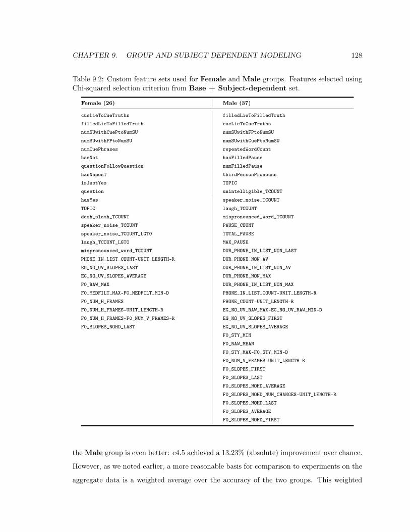
CHAPTER 9. GROUP AND SUBJECT DEPENDENT MODELING 128
Table 9.2: Custom feature sets used for Female and Male groups. Features selected usingChi-squared selection criterion from Base + Subject-dependent set.
Female (26) Male (37)
cueLieToCueTruths filledLieToFilledTruth
filledLieToFilledTruth cueLieToCueTruths
numSUwithCuePtoNumSU numSUwithFPtoNumSU
numSUwithFPtoNumSU numSUwithCuePtoNumSU
numCuePhrases repeatedWordCount
hasNot hasFilledPause
questionFollowQuestion numFilledPause
hasNaposT thirdPersonPronouns
isJustYes TOPIC
question unintelligible_TCOUNT
hasYes speaker_noise_TCOUNT
TOPIC laugh_TCOUNT
dash_slash_TCOUNT mispronounced_word_TCOUNT
speaker_noise_TCOUNT PAUSE_COUNT
speaker_noise_TCOUNT_LGT0 TOTAL_PAUSE
laugh_TCOUNT_LGT0 MAX_PAUSE
mispronounced_word_TCOUNT DUR_PHONE_IN_LIST_NON_LAST
PHONE_IN_LIST_COUNT-UNIT_LENGTH-R DUR_PHONE_NON_AV
EG_NO_UV_SLOPES_LAST DUR_PHONE_IN_LIST_NON_AV
EG_NO_UV_SLOPES_AVERAGE DUR_PHONE_NON_MAX
F0_RAW_MAX DUR_PHONE_IN_LIST_NON_MAX
F0_MEDFILT_MAX-F0_MEDFILT_MIN-D PHONE_IN_LIST_COUNT-UNIT_LENGTH-R
F0_NUM_H_FRAMES PHONE_COUNT-UNIT_LENGTH-R
F0_NUM_H_FRAMES-UNIT_LENGTH-R EG_NO_UV_RAW_MAX-EG_NO_UV_RAW_MIN-D
F0_NUM_H_FRAMES-F0_NUM_V_FRAMES-R EG_NO_UV_SLOPES_FIRST
F0_SLOPES_NOHD_LAST EG_NO_UV_SLOPES_AVERAGE
F0_STY_MIN
F0_RAW_MEAN
F0_STY_MAX-F0_STY_MIN-D
F0_NUM_V_FRAMES-UNIT_LENGTH-R
F0_SLOPES_FIRST
F0_SLOPES_LAST
F0_SLOPES_NOHD_AVERAGE
F0_SLOPES_NOHD_NUM_CHANGES-UNIT_LENGTH-R
F0_SLOPES_NOHD_LAST
F0_SLOPES_AVERAGE
F0_SLOPES_NOHD_FIRST
the Male group is even better: c4.5 achieved a 13.23% (absolute) improvement over chance.
However, as we noted earlier, a more reasonable basis for comparison to experiments on the
aggregate data is a weighted average over the accuracy of the two groups. This weighted

CHAPTER 9. GROUP AND SUBJECT DEPENDENT MODELING 129
Table 9.3: Local lie performance on 10 × 10-fold cross-validation Grouped by Gender
using Best 39 feature set from aggregate data and custom sets for groups, selected, using
Chi-squared selection criterion, from Base + Subject-dependent set.
Female (Chance=58.84) Male (Chance=61.24)
39 Features 26 Features 39 Features 37 Features
Ripper c4.5 Ripper c4.5 Ripper c4.5 Ripper c4.5
Accuracy 64.60 66.74 64.37 67.49 72.77 74.47 71.70 73.85
St. Err. 0.62 0.65 0.66 0.58 0.61 0.60 0.62 0.68
T F-measure 72.56 72.72 72.29 73.44 79.52 79.68 78.81 78.99
St. Err. 0.62 0.58 0.61 0.47 0.53 0.50 0.56 0.58
L F-measure 49.85 57.38 49.79 58.07 59.17 65.61 57.12 65.37
St. Err. 1.11 0.96 1.32 0.93 1.09 0.87 1.23 0.90
average for the c4.5 classifier is 70.67%, and is statistically identical to the prior best results
on the aggregate corpus, 70.00% vs. a baseline of 59.93%. An examination of the tree
learned for the Female group shows that it is not markedly different from trees learned in
earlier experiments: the subject-dependent features dominate the top-level nodes, while F0
features, and less frequently, lexical features, appear in the leaf nodes. The tree learned by
c4.5 on the Best 39 set for the Male group again uses subject dependent features on the
top level nodes. Leaf nodes show prominent use of pitch and energy features, as well as
discourse features such as cue phrases, specific denials, and questions. Interestingly, positive
and negative emotion words — particularly the former — appear at many leaves, and these
features were not selected in the custom set for this group. This again suggests that c4.5 is
able to infer more complex relationships than the univariate Chi-squared selection criterion
is able to exploit.1
1Although here, as in previous chapters, we attempted to employ a greedy feature selection algorithm
but were less successful than with Chi-squared ranking.
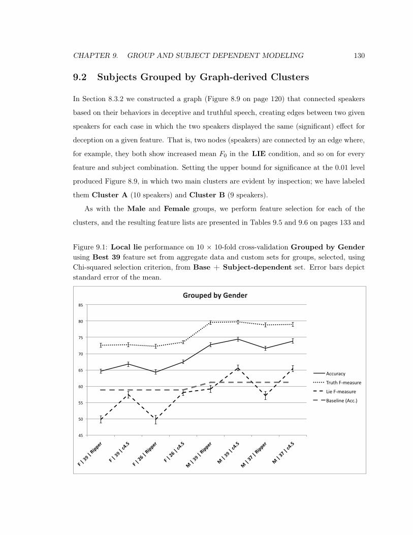
CHAPTER 9. GROUP AND SUBJECT DEPENDENT MODELING 130
9.2 Subjects Grouped by Graph-derived Clusters
In Section 8.3.2 we constructed a graph (Figure 8.9 on page 120) that connected speakers
based on their behaviors in deceptive and truthful speech, creating edges between two given
speakers for each case in which the two speakers displayed the same (significant) effect for
deception on a given feature. That is, two nodes (speakers) are connected by an edge where,
for example, they both show increased mean F0 in the LIE condition, and so on for every
feature and subject combination. Setting the upper bound for significance at the 0.01 level
produced Figure 8.9, in which two main clusters are evident by inspection; we have labeled
them Cluster A (10 speakers) and Cluster B (9 speakers).
As with the Male and Female groups, we perform feature selection for each of the
clusters, and the resulting feature lists are presented in Tables 9.5 and 9.6 on pages 133 and
Figure 9.1: Local lie performance on 10 × 10-fold cross-validation Grouped by Gender
using Best 39 feature set from aggregate data and custom sets for groups, selected, using
Chi-squared selection criterion, from Base + Subject-dependent set. Error bars depict
standard error of the mean.
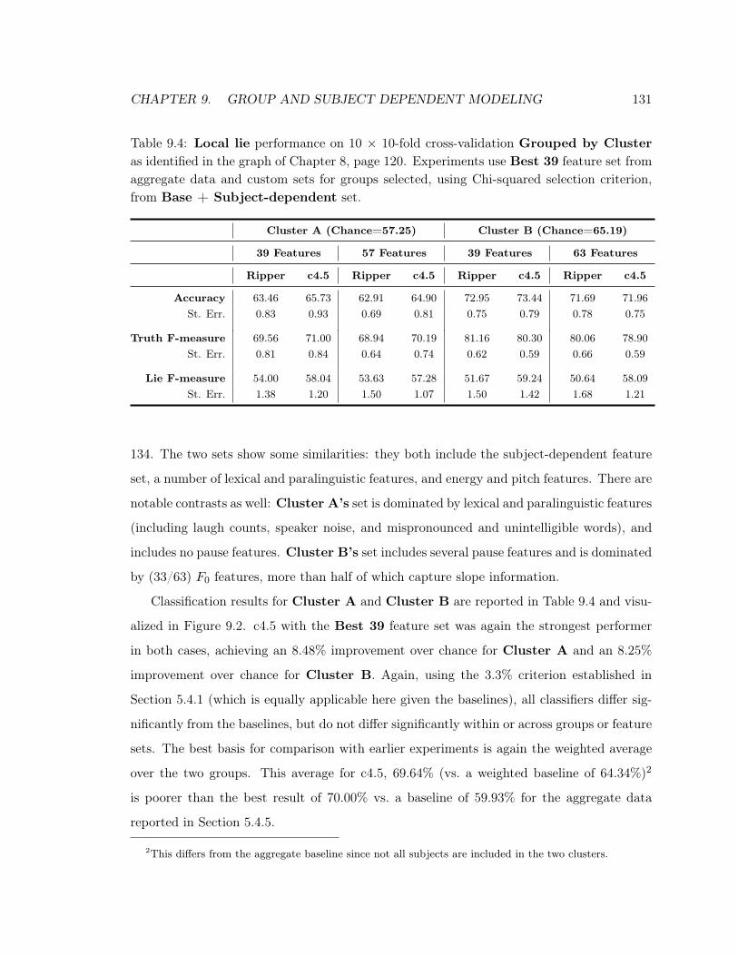
CHAPTER 9. GROUP AND SUBJECT DEPENDENT MODELING 131
Table 9.4: Local lie performance on 10 × 10-fold cross-validation Grouped by Cluster
as identified in the graph of Chapter 8, page 120. Experiments use Best 39 feature set from
aggregate data and custom sets for groups selected, using Chi-squared selection criterion,
from Base + Subject-dependent set.
Cluster A (Chance=57.25) Cluster B (Chance=65.19)
39 Features 57 Features 39 Features 63 Features
Ripper c4.5 Ripper c4.5 Ripper c4.5 Ripper c4.5
Accuracy 63.46 65.73 62.91 64.90 72.95 73.44 71.69 71.96
St. Err. 0.83 0.93 0.69 0.81 0.75 0.79 0.78 0.75
Truth F-measure 69.56 71.00 68.94 70.19 81.16 80.30 80.06 78.90
St. Err. 0.81 0.84 0.64 0.74 0.62 0.59 0.66 0.59
Lie F-measure 54.00 58.04 53.63 57.28 51.67 59.24 50.64 58.09
St. Err. 1.38 1.20 1.50 1.07 1.50 1.42 1.68 1.21
134. The two sets show some similarities: they both include the subject-dependent feature
set, a number of lexical and paralinguistic features, and energy and pitch features. There are
notable contrasts as well: Cluster A’s set is dominated by lexical and paralinguistic features
(including laugh counts, speaker noise, and mispronounced and unintelligible words), and
includes no pause features. Cluster B’s set includes several pause features and is dominated
by (33/63) F0 features, more than half of which capture slope information.
Classification results for Cluster A and Cluster B are reported in Table 9.4 and visu-
alized in Figure 9.2. c4.5 with the Best 39 feature set was again the strongest performer
in both cases, achieving an 8.48% improvement over chance for Cluster A and an 8.25%
improvement over chance for Cluster B. Again, using the 3.3% criterion established in
Section 5.4.1 (which is equally applicable here given the baselines), all classifiers differ sig-
nificantly from the baselines, but do not differ significantly within or across groups or feature
sets. The best basis for comparison with earlier experiments is again the weighted average
over the two groups. This average for c4.5, 69.64% (vs. a weighted baseline of 64.34%)2
is poorer than the best result of 70.00% vs. a baseline of 59.93% for the aggregate data
reported in Section 5.4.5.
2This differs from the aggregate baseline since not all subjects are included in the two clusters.

CHAPTER 9. GROUP AND SUBJECT DEPENDENT MODELING 132
Figure 9.2: Local lie performance on 10 × 10-fold cross-validation Grouped by Cluster
as identified in the graph of Chapter 8, page 120. Experiments use Best 39 feature set from
aggregate data and custom sets for groups selected, using Chi-squared selection criterion,
from Base + Subject-dependent set. Error bars depict standard error of the mean.
With respect to the trees learned for the clusters, for Cluster A we again see top-
level nodes that are dominated by subject-dependent, and some topic, features. The nodes
appear to be dominated by energy slope, pitch slope, durational and cue phrase related
features. Although these features all participate in complicated subtrees, one can generalize
that fewer cue phrases seem to point toward deception; increased phone duration points
toward truthfulness, and increased variability in pitch and energy tends to point toward
deception. Although caution is warranted given the complexity of the trees and the reliance
upon inspection to draw these inferences, these last three observations are consistent with
our hypothesis in Chapter 8 that the speakers of Cluster A are more animated in the
LIE condition.
Cluster B’s model is again dominated at the top level by subject-dependent and topic
features. Energy and pitch change features and durational features again appear frequently

CHAPTER 9. GROUP AND SUBJECT DEPENDENT MODELING 133
Table 9.5: Custom feature set (57 features) used for Cluster A. Features selected usingChi-squared selection criterion from Base + Subject-dependent set.
Feature Names
cueLieToCueTruths DUR_PHONE_IN_LIST_NON_MAX
filledLieToFilledTruth PHONE_COUNT-UNIT_LENGTH-R
numSUwithFPtoNumSU PHONE_COUNT
numSUwithCuePtoNumSU EG_NO_UV_SLOPES_FIRST
gender EG_NO_UV_STY_MAX-EG_NO_UV_STY_MIN-D
numCuePhrases EG_NO_UV_SLOPES_AVERAGE
hasCuePhrase EG_NO_UV_SLOPES_LAST
verbWithIng EG_NO_UV_NUM_R_FRAMES
hasI EG_NO_UV_RAW_MAX-EG_NO_UV_RAW_MIN-D
hasNot EG_NO_UV_SLOPES_NUM_CHANGES
thirdPersonPronouns F0_STY_MAX
hasPositiveEmotionWord F0_MEDFILT_MAX-F0_MEDFILT_MIN-D
noYesOrNo F0_RAW_MAX-F0_RAW_MIN-D
hasContraction F0_RAW_MIN
hasNaposT F0_NUM_H_FRAMES
hasNegativeEmotionWord F0_RAW_MAX
isJustYes F0_NUM_H_FRAMES-F0_NUM_V_FRAMES-R
hasWe F0_NUM_H_FRAMES-UNIT_LENGTH-R
isJustNo F0_STY_MAX-F0_STY_MIN-D
hasYes F0_SLOPES_MAX_NEG
hasAbsolutelyReally F0_SLOPES_NOHD_FIRST
specificDenial F0_SLOPES_LENGTH_LAST-UNIT_LENGTH-R
TOPIC F0_SLOPES_NOHD_LENGTH_LAST-UNIT_LENGTH-R
unintelligible_TCOUNT_LGT0 F0_SLOPES_LAST
laugh_TCOUNT F0_SLOPES_LENGTH_FIRST-UNIT_LENGTH-R
laugh_TCOUNT_LGT0 F0_SLOPES_AVERAGE
speaker_noise_TCOUNT F0_SLOPES_NOHD_LENGTH_FIRST-UNIT_LENGTH-R
speaker_noise_TCOUNT_LGT0 F0_SLOPES_NOHD_NUM_CHANGES
mispronounced_word_TCOUNT
in leaf nodes, and in this case the direction of correlation with deception is more evenly
distributed: although it appears that in the bulk of subtrees, these features correlate with
TRUTH (suggesting greater variability of speech in the TRUTH condition), there are
a fair number of subtrees in which the opposite is true, suggesting the possibility that
subclasses of speaking styles are being treated differently by the model.
We had hoped that the models for these clusters, being empirically derived via our
subject-dependent statistical analyses, might have outperformed the aggregate speaker set

CHAPTER 9. GROUP AND SUBJECT DEPENDENT MODELING 134
Table 9.6: Custom feature set (63 features) used for Cluster B. Features selected usingChi-squared selection criterion from Base + Subject-dependent set.
Feature Names
filledLieToFilledTruth F0_STY_MAX
cueLieToCueTruths F0_MEDFILT_MAX-F0_MEDFILT_MIN-D
numSUwithFPtoNumSU F0_STY_MAX-F0_STY_MIN-D
numSUwithCuePtoNumSU F0_STY_MIN
gender F0_RAW_MAX-F0_RAW_MIN-D
numFilledPause F0_NUM_R_FRAMES
hasSelfRepair F0_NUM_F_FRAMES
hasI F0_NUM_V_FRAMES
thirdPersonPronouns F0_RAW_MAX
repeatedWordCount F0_STY_MEAN
TOPIC F0_NUM_F_FRAMES-F0_NUM_V_FRAMES-R
NUM_WORDS F0_NUM_F_FRAMES-UNIT_LENGTH-R
mispronounced_word_TCOUNT F0_SLOPES_NOHD_NUM_CHANGES
dash_slash_TCOUNT F0_SLOPES_LENGTH_LAST-UNIT_LENGTH-R
breath_TCOUNT F0_SLOPES_NOHD_LAST
UNIT_LENGTH F0_SLOPES_AVERAGE
TOTAL_PAUSE-UNIT_LENGTH-R F0_SLOPES_MAX_POS
TOTAL_PAUSE F0_SLOPES_NOHD_FIRST
PAUSE_COUNT F0_SLOPES_NOHD_AVERAGE
MAX_PAUSE F0_SLOPES_NOHD_MAX_POS
DUR_PHONE_IN_LIST_NON_AV F0_SLOPES_LAST
PHONE_IN_LIST_COUNT F0_SLOPES_FIRST
PHONE_COUNT F0_SLOPES_MAX_NEG
EG_NO_UV_SLOPES_FIRST F0_SLOPES_NOHD_MAX_NEG
EG_NO_UV_SLOPES_LAST F0_SLOPES_NOHD_NUM_CHANGES-UNIT_LENGTH-R
EG_NO_UV_NUM_F_FRAMES F0_SLOPES_LENGTH_FIRST
EG_NO_UV_NUM_R_FRAMES F0_SLOPES_NOHD_LENGTH_FIRST-UNIT_LENGTH-R
EG_NO_UV_RAW_MAX-EG_NO_UV_RAW_MIN-D F0_SLOPES_NOHD_LENGTH_FIRST
EG_NO_UV_SLOPES_NUM_CHANGES F0_SLOPES_NOHD_LENGTH_LAST-UNIT_LENGTH-R
EG_NO_UV_SLOPES_AVERAGE F0_SLOPES_LENGTH_FIRST-UNIT_LENGTH-R
F0_RAW_MEAN F0_SLOPES_NOHD_LENGTH_LAST
F0_RAW_MIN
or other groups examined. Some clue as to why this is not the case might be found in the
high degree of variability across experiments evidenced in the relatively high standard errors
reported in Table 9.4. Although we find in the learned models some evidence to support
our hypotheses in Chapter 8 regarding differences in degree of animation between the de-
ceptive speech of the two groups, the high S.E. we find among the experiments suggests

CHAPTER 9. GROUP AND SUBJECT DEPENDENT MODELING 135
a high degree of variability among the speakers with respect to the efficacy of the more
complicated classification and regression trees produced by c4.5. This points perhaps to
the limitations of the univariate statistical analyses applied in deriving the clusters. Upon
making this observation, we did, in fact, return to the data and test the efficacy of logistic
regression classifiers on the clusters, thinking perhaps that they were better suited to cap-
turing the effects inherent in the two groups. In preliminary experiments, however, they
performed consistently worse than the classifiers reported on here, again suggesting that the
phenomenon we study is a matter of complex interplay among the features.
9.3 Another Approach to Speaker Similarity
In addition to the grouping approaches reported above, we experimented with a technique
from the speaker verification domain whereby “close” speakers are identified and pooled
to create higher likelihood background models (Reynolds, 1997). With this technique, a
pairwise comparison is performed to identify speakers whose maximum-likelihood models
perform well on one another’s data. Thus, given utterances XA and XB from speaker
models λA and λB, distance between the two speaker models is defined as
d(λA, λB) = log
{
p(XA|λA)
p(XA|λB)·p(XB|λB)
p(XB|λA)
}
.
We apply a similar approach with the speakers of the CSC Corpus in order to pool speakers
who have similar deceptive speech behaviors. Here, we use as our performance metric for
a given model the harmonic mean of: raw accuracy and F-measure with respect to LIE.
These two raw metrics capture the two most salient performance measures, and using their
harmonic mean penalizes cases where one metric is substantially lower than the other. Our
distance measure for speakers A and B thus becomes
d(A, B) = log
{
1
HAB
·1
HBA
}
,
where HAB is the harmonic mean of the accuracy and F-measure obtained by applying the
SVM model trained on speaker B to data from speaker A. We use 1 as the numerator here
(as opposed to e.g. HAA) since comparing to 1 reflects comparison to optimal performance.
We perform pairwise comparisons of all subjects using this distance metric, and then group

CHAPTER 9. GROUP AND SUBJECT DEPENDENT MODELING 136
Table 9.7: c4.5 performance on grouped speakers
Loose equivalence classes
# Spkrs. Improvement Accuracy F-measure Baseline
21 10.83 63.87 0.614 53.04
3 -3.21 61.60 0.421 64.41
2 17.82 69.87 0.687 52.05
Strict equivalence classes
# Spkrs. Improvement Accuracy F-measure Baseline
5 8.50 68.82 0.758 60.32
4 7.39 59.33 0.600 51.94
2 0.20 68.11 0.465 67.91
2 17.82 69.87 0.687 52.05
2 6.32 72.33 0.575 66.01
2 2.13 53.81 0.512 51.68
speakers whose distance does not exceed a given threshold; results reported here use a
threshold of 1.5.
In the experiments described here, classification models for the local lie category are
trained for each speaker, using various learning algorithms. Results for these models are
used to evaluate the existence of similar speakers; these similar models are in turn combined
to create group models as described below. In all cases, best results are obtained using either
support vector machines (SVM) (Boser, Guyon & Vapnik, 1992) with a radial basis function
kernel as implemented in Weka, or using J48, Weka’s implementation of c4.5(Quinlan, 1986),
as indicated.
We use two strategies to group speakers, creating two kinds of equivalence classes. In
both approaches a class initially contains one pair of “close” speakers. Loose equivalence
classes are built by adding subsequent speakers if they were close to at least one member
of an existing class. Strict equivalence classes are built as follows: speaker A is added to
an existing class only if A is close to all current members of the class, enforcing a transitive

CHAPTER 9. GROUP AND SUBJECT DEPENDENT MODELING 137
relationship with respect to distance within each class. Although this approach produces
many more small groups, performance is comparable. In this manner, using a threshold
of 1.5, 3 loose groups and 6 strict groups are created. Models are trained and tested for
the combined data of the resulting groups using both SVMs and c4.5 with 10-fold cross-
validation. c4.5 achieves superior performance, and results are reported in Table 9.7. Both
on average and for most groups, performance compares favorably with that of the aggregate
data. Weighted average improvement (by number of speakers per group) for strict groups is
7.35%; weighted average F-measure is .628. Averages for loose groups are 9.75% and .597.
F-measures reported here also compare favorably with performance on the aggregate data.
9.3.1 Discussion
It would seem intuitive to expect that strict groups would show better performance than
loose groups. In practice we find that performance is roughly similar, with loose groups
showing higher average gain over baseline but lower average F-measure. This is likely due
to the fact that the similarity of individual subjects in the strict groups is balanced by the
greater amount of training data for the largest of the loose groups (interestingly however, the
same two-speaker group that showed the highest gain (17.82%) was present in both types
of grouping).
We examined c4.5 classification and regression trees for all groups evaluated in order
to gain some insight with respect to cues to deception. For subjects who showed positive
improvement over baseline using subject-dependent models, we found that in all cases, top-
level rules involved lexical or lexically related features, such as the presence of not, we,
questions and mispronunciations. These are all consistent with hypotheses in the literature,
and here may capture individual styles of deceptive behavior. Lower level rules made heavy
use of automatically extracted prosodic features. Models for loose groups made use of top-
level rules involving subject-dependent features, such as numbers of cue phrases presence
of questions, and presence of unintelligible words, which may speak to the idea of vocal
immediacy or directness posited by DePaulo et al. (DePaulo et al., 2003). Interestingly,
the top-level rules for the strict groups make use of all features mentioned above, with
the addition of gender and the presence of specific denials, a feature borrowed from field

CHAPTER 9. GROUP AND SUBJECT DEPENDENT MODELING 138
Table 9.8: Local lie performance on single speakers for background models, single-speaker
models, and human judges.
Classifier Impvt. over Baseline Std. Dev. LIE F-measure Std. Dev.
Background -1.23 3.53 30.02 30.05
Single-speaker -2.80 6.84 41.04 21.37
Human -8.39 10.89 35.45 12.42
practitioners (Reid & Associates, 2000). All models make use of the presence of positive
and negative emotion words (cf. (Whissel, 1989)).
9.4 Speaker-dependent Models
The work we have reported thus far on group and individual differences points to the pos-
sibility of performing strictly within-subject classification. Although the resulting small
sample sizes do not lead us to expect strong performance, we nevertheless thought it of
some interest to test performance on individual speakers. We segregate and examine speak-
ers in two ways: first, individual SVM models are trained and evaluated for each speaker
using leave-one-out cross-validation in individual segments in order to maximize the avail-
able training data. Second, for the purposes of comparison, we devised a complementary
task: “background” SVM models (we borrow terminology from the speaker verification do-
main) are built, using 31/32 speakers as training data, and then evaluated on the speaker
that was omitted from the training data. In this way, we examine both speaker-dependent
models and the performance of general models on unknown speakers.
Results are displayed in Figure 9.8, along with comparable results for humans classifying
local lies (humans performed on average worse than chance at this task; we report this in
detail in Chapter 10). We primarily consider two metrics: improvement over the chance base-
line, and F-measure using LIE as the category of interest. These metrics are of interest since
raw accuracy is not comparable across subjects because each subject’s class TRUTH/LIE
priors varied, and since the ability to detect lies is well reflected by balancing precision and

CHAPTER 9. GROUP AND SUBJECT DEPENDENT MODELING 139
recall via F-measure. Speaker-dependent models perform better than background models in
terms of number and magnitude of positive gain over chance. F-measure is also greater for
speaker-dependent models (Wilcoxon paired signed rank test: p-value < 0.001). Improve-
ment over baseline of subject-dependent models exceeds that of human judges (Wilcoxon
paired signed rank test: p-value = 0.009). The relative performance of humans and the two
models on an individual speaker basis is best illustrated by two bar-graphs, Figures 9.3 and
9.4 on pages 142 and 143.
There are a number of observations to be made regarding both the graphs and the
aggregate statistics. First, it is curious that the magnitude of standard deviation for the two
measures is ordered differently with respect to the classifiers; that is, the background models
show the lowest variance, and humans the highest, with respect to accuracy improvement
over baseline, while the background models demonstrate the greatest variance for F-measure,
and humans the lowest. One possible explanation is that, while the background models (and
possibly the single speaker models) rely upon inferring the class distribution in the data,
and subsequently guessing the majority class more often (explaining an average improvement
near 0.0), humans could not infer this distribution and assigned labels without the advantage
of that knowledge. This also helps to explain the statistics with regard to F-measure: Figure
9.4 reveals that in many cases the background model identifies none of the LIE segments,
indicating that it labeled every segment with the majority class. Additionally, there is some
possibility that the consistency of humans’ F-measure scores is related to what is known as
“truth bias” on the part of naive hearers (Vrij, 2008), whereby individuals have a relatively
consistent expectation with respect to the likelihood with which others will lie. Such a bias
would lead one to expect a fairly consistent level of performance with respect to F-measure.
An examination of the two bar graphs reveals that performance was fairly consistent
across “classifiers”. That is, where one did well, the other two seemed to as well; where
one did poorly, so, often, did the others. It is reasonable to think that, in the case of
the background models, subjects whose behaviors were more similar to others were more
easily classified; perhaps, too, the behavior of these subjects was recognized as familiar by
the human judges. It is also interesting that this is one of the few cases we encountered
with the corpus in which SVM classification was the preferred choice (we found that other

CHAPTER 9. GROUP AND SUBJECT DEPENDENT MODELING 140
classifiers performed even more poorly); it is possible that limiting the data as we did made
it more difficult to take advantage of the sorts of complex relationships among features that
we observed in Chapter 5. Finally, having seen the improved performance with respect to
the normalized subset of data used in Chapter 5, it may be worth revisiting the idea of
single-speaker models in future work, despite the limited amount of data available to do so.
9.5 Conclusions and Future Work
Both in the case of subject-dependent and group-dependent models, performance for certain
individuals and groups shows considerable gains over the baseline. This is true for the group
of Male subjects, where the best accuracy relative to chance and best LIE F-measure was
achieved for any experiments on the corpus. As we detailed above, however, we are hesitant
to make strong claims about the efficacy of group modeling, since when results of the groups
are combined using weighted averages, they do not improve upon performance realized on
the aggregate data.
As we described above, we had hoped that the empirically derived clusters might help to
achieve better performance than that realized on the aggregate data. Although the models
learned show some evidence to support our hypotheses in Chapter 8 regarding different
deceptive speech styles between the two groups, the high S.E. we find among the experiments
for each group suggests a high degree of variability among the speakers, possibly making it
difficult to induce a model applicable to the entire cluster. This in turn suggests limitations
with respect to the univariate statistical analyses applied in deriving the clusters, especially
given the capacity of c4.5 to model complex dependencies.
Substantial gains were also realized for some of the distance-measure-derived groups of
Section 9.3, suggesting that this approach might be worth revisiting in future work using
the more recent normalized feature set. Of course, given unlimited data, speaker-dependent
models would likely be optimal. In the case of an unseen speaker, however, a promising
strategy would be to apply a classifier trained on speakers expected to behave similarly to
the new speaker. This is straightforward for grouping by gender, of course. And given some
training data for a new speaker, it might be possible to assign a model to that speaker

CHAPTER 9. GROUP AND SUBJECT DEPENDENT MODELING 141
using either one of the clustering approaches presented in this chapter if the efficacy of
the classifiers for those groups could be increased sufficiently to warrant doing so. An
interesting next step would be to attempt to identify speakers that fit a particular model
by clustering or identification of behaviors common to members of a group without recourse
to TRUTH / LIE labels. For example, we reported in Section 8.3.2 that more animated
speech is indicative of deception for speakers of Cluster A. Perhaps it is the case that
great variance for a given speaker in the relevant features, such as maximum positive pitch
slope, number of rising frames, or count of laughs, is itself indicative of membership in
Cluster A. Likewise, perhaps certain generalized behaviors with respect to Cluster B’s
significant features, such as minimum pitch, vowel duration, and count of falling frames, are
indicative of membership in this cluster. These ideas of course require testing, but in this
chapter and in Section 8.3.2 we have identified a number of group dependent behaviors and
thus have taken a useful first step in this process.

CHAPTER 9. GROUP AND SUBJECT DEPENDENT MODELING 142
Figure 9.3: Local lie classification performance: improvement over chance baseline, by
speaker; performance for human judges, background models, and single-subject models.

CHAPTER 9. GROUP AND SUBJECT DEPENDENT MODELING 143
Figure 9.4: Local lie classification performance: LIE F-measure, by speaker; performance
for human judges, background models, and single-subject models.

PART IV. 144
Part IV
Human Deception Detection

Chapter 10. 145
Chapter 10
Human Deception Detection and the
CSC Corpus: A Perception Study
In this chapter, we describe a perception study (first reported in (Enos, Benus, Cautin,
Graciarena, Hirschberg & Shriberg, 2006)) in which judges attempted to classify as decep-
tive or truthful the interviews that compose the CSC Corpus on both the global lie and
local lie levels. Our review of the literature on deception detection revealed to us the low
degree — generally near chance — to which humans are able to accurately discriminate
between truthful and deceptive behavior. The performance of these human judges helps to
contextualize the results we have reported in the preceding chapters for automatic decep-
tion detection. In addition, we report a number of strong results suggesting that particular
personality factors may contribute significantly to a judge’s success at classification.
10.1 Previous Research
We reviewed in Chapter 2 a number of findings regarding human performance at deception
detection. The reader will recall that, in general, people perform very poorly at this task,
with most groups, trained and untrained, performing at or near chance. A recent meta-
analysis (Aamodt & Custer, 2006) examines the results of 108 studies that attempted to
determine if individual differences exist in the ability to detect deception. Ability (where
chance is 50%) ranged from that of parole officers (40.41%, one study) to that of secret

CHAPTER 10. HUMAN DECEPTION DETECTION AND THE CSC CORPUS 146
service agents, teachers, and criminals (one study each) who scored in the 64–70% range.
The bulk of studies (156) used students as judges; they scored on average 54.22%. A meta-
analysis by Bond and DePaulo (2006) examining “hundreds of experiments” likewise finds
that the mean accuracy of perceivers is 54%. In a subset of studies they found that perceivers
who judged exclusively audio data performed better (53.01% on average) than those who
judged exclusively video data (50.5%).
10.2 Procedure
For the perception study, we recruited thirty-two native speakers of American English (re-
ferred to in this chapter as “judges” in order to avoid confusion with respect to the appellation
“subject”) from the community and from the Columbia University student population to par-
ticipate in a “communication experiment” in exchange for payment.1 Each judge listened
to two complete interviews from the CSC Corpus that were selected in order to balance
the length of interviews as much as possible (i.e., one long, one short) so that judges could
complete the task within two hours. Judges were asked to indicate their judgments on both
local and global lies for these interviews. They labeled local truth and local lie via a
labeling interface constructed in Praat2 (Boersma & Weenink, 2006). Judges were able to
replay sections at will. They indicated their judgments with respect to global truth / lie
(that is, the speakers’ claimed score in each section) on a paper form. For one of the two
interviews, each judge received a section of training, or immediate feedback, with respect to
the correctness of his or her judgments, so that we could test the effect of training on their
judgments (see below). Each judge rated two speakers and each speaker was rated by two
judges.
So that we could examine individual differences among judges, prior to the perception
task judges were administered the NEO-FFI form, measuring the Costa & McCrae five-factor
personality model, a widely used personality inventory for nonclinical populations (Costa
1This human subjects study was authorized by the approval of Columbia University IRB Protocol IRB-
AAAA3595.
2Here judges labeled segments delimited by speaker pedal presses, as described in Section 3.

CHAPTER 10. HUMAN DECEPTION DETECTION AND THE CSC CORPUS 147
& McCrae, 1992; Costa & McCrae, 2002). The five-factor model is an empirically-derived
and comprehensive taxonomy of personality traits. It was developed by applying factor
analysis to thousands of descriptive terms found in a standard English dictionary. Five
personality dimensions emerged: Openness to Experience, Conscientiousness, Extraversion,
Agreeableness, and Neuroticism. This model and associated measures appear extensively in
the psychology literature. We describe the model and the NEO-FFI in detail in Section 10.5.
Judges next filled out a brief questionnaire that asked if they had work experience in
which detecting deception was relevant and, if so, to describe that experience. They were
also asked to respond on a five-point Likert scale to questions intended to determine their
preconceptions with respect to lying (How often can you spot a lie in daily life? and How
often do you think people lie in daily life in order to achieve some undeserved gain, either
material or social? ).
Next, judges received written and oral instructions on the perception task: the CSC
Corpus was described to them in layman’s terms; then, the task and method of labeling
each section (global lies) and each segment ( local lies) was explained.
Each judge received “training” for one section of one of the interviews judged. The train-
ing consisted of immediate feedback via the interface on the correctness of their ratings.
Specifically, the labeling interface indicated “correct” or “incorrect” for each judgment pro-
duced by the judge at the local lie level for one entire interview section for one subject; the
judge’s conclusion with respect to the global lie for that section was discarded for the pur-
poses of the study, since the reference local lie labels for the relevant segments necessarily
reveal the speaker’s veracity at the global lie level. Training was balanced: odd-numbered
judges received training on the first speaker and even-numbered judges on the second in
order to account for any practice effect. (No such effect was subsequently detected.) In both
even and odd cases the judge received training on a section in which the speaker lied about
his or her performance.
After judging two interviews, judges were asked Did you find it easy to use the interface?
(all judges responded yes). Judges were also asked to rate their confidence on their perfor-
mance: In your opinion, how many of the judgments you made today are correct? Again,
judges responded on a five-point Likert scale, for both local lie and global lie performance.

CHAPTER 10. HUMAN DECEPTION DETECTION AND THE CSC CORPUS 148
Table 10.1: Judges’ aggregate performance classifying TRUTH /LIE.
Lie Type Chancea Meanb Std. Dev. Min. Max. T F-meas. L F-meas.
Local 66.62 58.23 7.51 40.64 71.48 65.88 35.45
Global 62.55 47.76 14.82 16.67 75.00 42.87 46.80
aGuessing majority class each time.
bEach judge’s score is his or her average over two interviews; as percentages.
10.3 Results on Deception Detection
We now consider accuracy by examining each judge’s average performance over two inter-
views, the average performance of two judges on each speaker, and judges’ performance in
the context of machine learning results on the corpus. As noted in Section 10.1, previous
studies have shown that most of the population performs quite poorly at the deception de-
tection task. Our study on the CSC Corpus supports this conclusion. Table 10.1 shows the
aggregate performance of judges on both levels of TRUTH and LIE. No effect was found
for the length of the interview. Most notable is that judges performed worse than chance
on both local and global lies (where chance is understood to mean guessing the majority
class for the aggregate data, for the local level, always TRUTH and for the global level
almost always LIE). The data reflect considerable variability among judges, particularly
on the level of the global lie , where standard deviation is quite large, and the difference is
great between the best and worst performers. Likewise, the low maximum scores on both
levels point to the difficulty of the task.
In Chapter 5 we reported that our best machine accuracy classifying local lies was
70.00%, versus a chance baseline of 59.93% for SUs, with f-measure (evaluating for LIE) of
60.59. Although the present study focuses on pedal-press-defined units (as opposed to SUs),
comparison of results with respect to the difference between classification accuracy and base-
line, as well as f-measure, serve to relate human performance to machine performance. On
average, judges classified local lies with an accuracy of 58.23% versus a chance baseline of

CHAPTER 10. HUMAN DECEPTION DETECTION AND THE CSC CORPUS 149
Table 10.2: Aggregate performance by speaker.
Lie Type Chance Meana Std. Dev. Min. Max. T F-meas. L F-meas.
Local 66.62 58.23 9.44 35.86 87.79 65.88 35.45
Global 62.30 47.76 15.37 16.67 83.33 42.87 46.80
aEach speaker’s score is the average over two judges; as percentages.
66.62%, performing worse than chance. Judge’s f-measure with respect to LIE was compa-
rably poor, averaging 46.80. And again, although it is admittedly an imperfect comparison,
our performance classifying global lies, reported in Chapter 6, was approximately an 11%
absolute improvement over chance (albeit for the undersampled data distribution). Even
given the limitations of the comparison, we interpret the current finding — that humans
perform worse than chance on both levels of lie — to suggest that our machine learning
results are fairly good when compared to human performance.
We now consider the question of whether some speakers are more or less difficult for
people to classify. Although we hesitate to make strong statistical inferences in this respect
(since each interview was labeled by only two judges), a comparison of Table 10.2 with Table
10.1 provides some insight. Inspection shows that the range of scores on speakers is greater
than that of the range of scores among judges. In addition, these results suggest a greater
variance (shown as standard deviation) among speakers than among judges, both at the
local and global levels. This suggests to us that speakers in our study varied more in their
detectability than did individual judges in their ability to detect deception.
10.3.1 Additional findings
We considered a number of attributes of the judges to determine their salience in the de-
ception detection task. We considered, for example, if male subjects differed from female
subjects in deception detection ability. We found no significant effect at either level of lie
for gender, and this is consistent with existing literature. Aamodt and Custer (2006), for
example, found no significant differences between men and women in their meta-analysis

CHAPTER 10. HUMAN DECEPTION DETECTION AND THE CSC CORPUS 150
of deception detection studies. We likewise found no effects for age on deception detection
ability, and this is again consistent with the literature (Aamodt & Custer, 2006). We next
considered the prior experience of the judge at lie detection tasks. Our pre-test question-
naire asked judges to indicate if they had prior experience, and to describe that experience.
Seven of our subjects so self-identified, and reported seven different activities they believed
to be salient to the task: “Insurance claims examiner”, “Marines”, “Customer service repre-
sentative”, “Private investigator”, “EMT”, “Restaurant manager”, and “Retail”.
This evaluation necessarily relies on self-report, but it is worth noting that all of the oc-
cupations described could conceivably benefit from skill at lie-detection, and would possibly
present some opportunity to attempt to develop such skill.
Our subsequent analysis found that there was no effect for experience on a judge’s
performance. However, we found an interesting effect related to the judges’ confidence
in this regard. We attempted to assess judges’ confidence both pre-and post-task, and to
differentiate post-task between confidence in both local lie and global lie detection ability.
For this purpose, we asked subjects How often can you spot a lie in daily life? prior to the
task, and In your opinion, how many of the judgments you made today are correct? for
both local and global lies. For all three questions, judges responded on a five-point Likert
scale. A histogram of the judge responses to these questions is displayed in Figure 10.1.
The pre-task confidence of judges who reported experience was no higher than that of
judges reporting no experience (two-sample t-test, n.s.). This, again, is consistent with the
literature, which finds consistently that confidence is not related to accuracy (Aamodt &
Custer, 2006). However, while the confidence of inexperienced judges decreased from pre-
task to post-task for both the local lie (paired t-test: p.value=0.001; mean of differences
0.64) and global lie (paired t-test: p.value=0.020; mean of differences 0.48) levels, there was
no significant difference in confidence pre- and post-task for the judges claiming experience.3
This finding is consistent with existing literature on confidence, training, and experience
in deception detection. A number of studies (e.g. (Kassin, Meissner & Norwick, 2005) and
3We are fairly confident that this mitigates the difference in the wording of the questions, since if the
differences in confidence ratings were an artifact of different scales of responses attributable to the wording
of the question, we expect that that artifact would be evident in both groups.

CHAPTER 10. HUMAN DECEPTION DETECTION AND THE CSC CORPUS 151
Figure 10.1: Self-reported judge confidence of deception-detection ability, pre- and post-task
on a five-point Likert scale, where 5 is highest.
see (Kassin & Fong, 1999) for a review of literature on confidence in deception detection)
have shown that while police detectives perform no better than college students at deception
detection (and in some cases, worse (Kassin et al., 2005)), their level of confidence in their
judgments is consistently higher than other groups. Kassin and Fong (1999) found that
the ability of naive subjects to detect deception actually deteriorated with training in some
common methods used by police, while their confidence in their judgments and their ability
to justify their decisions increased. Finally, in their meta-analysis, Aamodt and Custer
(2006) found no differences between law enforcement professionals and others, and only a
slight advantage (mean 55.51%, N=2,685 vs. mean 54.22%, N=11,647) for “professional” lie
catchers (a group that included e.g. psychologists, secret service agents, parole officers and
judges along with police) over novices.
A related observation pertains to the sort of training provided in the present study. The
reader will recall that each judge received immediate feedback with respect to his or her

CHAPTER 10. HUMAN DECEPTION DETECTION AND THE CSC CORPUS 152
judgments on the local lie level for one section of one speaker. The purpose of this was to
provide feedback specific to one of the two speakers in order to test if the judge was able
to infer any relevant cues with respect to the given speaker’s method of deceiving. Our
analysis (paired t-test, n.s) found no difference in the judges’ performance on the speaker
for whom they received training, and order of the speaker (first or second) for which training
was provided had no effect on performance.
Detailed performance statistics for both levels of lie, by speaker and by judge, are found
in Figures 10.4, 10.3, 10.6, and 10.5. In the next section, we take up the possibility that the
detectability of subjects is predictable using automatic methods; at the end of this chapter,
we report a number of interesting findings related to the personality of judges and their
ability to detect deception.

CHAPTER 10. HUMAN DECEPTION DETECTION AND THE CSC CORPUS 153
Table 10.3: Global lie performance statistics by judge.
Judge Av. baseline Guessed Accuracy Improvement T F-meas. L F-meas. Gender Experience
J01 63.33 28.34 45.00 -18.33 48.57 40.00 F N
J02 63.33 36.67 56.67 -6.67 56.67 56.67 F N
J03 55.00 55.00 16.67 -38.34 16.67 16.67 M N
J04 63.33 45.00 61.67 -1.67 60.00 62.86 M N
J05 55.00 30.00 35.00 -20.00 33.34 16.67 F N
J06 63.33 81.67 61.67 -1.67 33.34 73.02 F N
J07 63.33 18.34 35.00 -28.33 45.24 20.00 M N
J08 63.33 28.34 28.34 -35.00 34.29 20.00 F N
J09 63.33 20.00 16.67 -46.67 25.00 0.00 F Y
J10 63.33 58.34 55.00 -8.33 28.57 57.50 F N
J11 63.33 56.67 53.34 -10.00 33.34 61.91 F N
J12 53.33 65.00 65.00 11.67 53.34 71.43 M N
J13 63.33 28.34 28.34 -35.00 34.29 20.00 M Y
J14 63.33 28.34 28.34 -35.00 34.29 20.00 M N
J15 63.33 45.00 45.00 -18.33 40.00 48.57 M N
J16 63.33 45.00 61.67 -1.67 60.00 62.86 F N
J17 63.33 55.00 35.00 -28.33 20.00 45.24 M N
J18 63.33 55.00 55.00 -8.33 45.00 61.91 F Y
J19 55.00 20.00 55.00 0.00 66.67 25.00 M N
J20 63.33 63.34 63.34 0.00 50.00 70.84 F N
J21 53.33 53.34 46.67 -6.67 33.34 50.00 M Y
J22 63.33 46.67 46.67 -16.67 41.67 50.00 M N
J23 63.33 26.67 26.67 -36.67 33.33 16.67 M N
J24 63.33 35.00 55.00 -8.33 53.34 53.57 M Y
J25 63.33 36.67 56.67 -6.67 56.67 56.67 M N
J26 63.33 45.00 65.00 1.67 60.00 68.57 F N
J27 63.33 56.67 53.34 -10.00 33.34 61.91 F N
J28 63.33 43.34 46.67 -16.67 33.34 50.00 F N
J29 63.33 63.34 46.67 -16.67 25.00 58.34 M N
J30 63.33 45.00 61.67 -1.67 60.00 62.86 M Y
J31 63.33 26.67 46.67 -16.67 50.00 41.67 F N
J32 63.33 41.67 75.00 11.67 73.34 76.19 F Y

CHAPTER 10. HUMAN DECEPTION DETECTION AND THE CSC CORPUS 154
Table 10.4: Global lie performance statistics by speaker.
Speaker Baseline Guessed Accuracy Improvement T F-meas. L F-meas.
S01 63.33 38.34 38.34 -25.00 39.29 33.34
S02 63.33 56.67 53.34 -10.00 33.34 61.91
S03 63.33 35.00 55.00 -8.33 53.34 53.57
S04 63.33 20.00 56.67 -6.67 65.00 40.00
S05 63.33 18.34 35.00 -28.33 45.24 20.00
S06 45.00 73.34 56.67 1.67 33.34 67.86
S07 63.33 38.34 35.00 -28.33 28.57 36.67
S08 63.33 45.00 65.00 1.67 60.00 68.57
S09 45.00 45.00 46.67 -8.33 50.00 41.67
S10 63.33 75.00 55.00 -8.33 20.00 66.07
S11 63.33 45.00 45.00 -18.33 40.00 48.57
S12 63.33 36.67 53.34 -10.00 53.34 53.34
S13 63.33 45.00 61.67 -1.67 60.00 62.86
S14 63.33 56.67 36.67 -26.67 16.67 45.24
S15 63.33 53.34 53.34 -10.00 45.00 57.50
S16 63.33 63.34 26.67 -36.67 0.00 41.67
S17 63.33 28.34 65.00 1.67 68.57 60.00
S18 63.33 45.00 45.00 -18.33 40.00 48.57
S19 45.00 20.00 55.00 0.00 66.67 25.00
S20 45.00 30.00 25.00 -30.00 33.34 0.00
S21 63.33 46.67 46.67 -16.67 41.67 50.00
S22 63.33 50.00 83.33 20.00 80.00 85.71
S23 63.33 35.00 55.00 -8.33 53.34 53.57
S24 63.33 38.34 38.34 -25.00 39.29 33.34
S25 63.33 36.67 36.67 -26.67 36.67 36.67
S26 63.33 36.67 16.67 -46.67 16.67 16.67
S27 63.33 53.34 36.67 -26.67 20.00 45.00
S28 63.33 71.67 71.67 8.33 58.34 77.78
S29 63.33 26.67 26.67 -36.67 33.33 16.67
S30 63.33 56.67 53.34 -10.00 33.34 61.91
S31 63.33 28.34 28.34 -35.00 34.29 20.00
S32 63.33 35.00 71.67 8.33 73.34 67.86

CHAPTER 10. HUMAN DECEPTION DETECTION AND THE CSC CORPUS 155
Table 10.5: Local lie performance statistics by judge.
Judge Av. baseline Guessed Accuracy Improvement T F-meas. L F-meas. Gender Experience
J01 54.86 59.41 56.90 2.03 66.64 38.56 F N
J02 72.50 64.37 56.41 -16.09 67.33 27.36 F N
J03 73.72 69.17 65.69 -8.02 77.54 25.22 M N
J04 75.83 76.71 69.44 -6.40 77.79 50.37 M N
J05 67.64 47.66 40.64 -27.00 41.75 39.02 F N
J06 72.95 50.62 49.97 -22.98 60.02 33.17 F N
J07 75.44 52.21 70.84 -4.60 81.49 8.33 M N
J08 61.09 43.75 47.88 -13.22 54.38 37.16 F N
J09 59.62 48.06 59.41 -0.22 70.13 27.66 F Y
J10 53.82 55.56 57.95 4.13 68.18 35.98 F N
J11 62.70 48.25 53.60 -9.10 57.95 47.61 F N
J12 60.76 48.05 50.31 -10.45 57.12 40.78 M N
J13 72.12 61.40 60.11 -12.01 73.44 19.58 M Y
J14 69.58 57.25 62.45 -7.13 75.42 20.46 M N
J15 70.75 64.95 66.22 -4.53 74.55 36.43 M N
J16 62.48 54.44 54.34 -8.14 57.07 46.45 F N
J17 54.86 61.07 59.52 4.66 63.82 54.04 M N
J18 72.50 53.96 56.12 -16.39 64.80 38.81 F Y
J19 73.72 55.74 61.53 -12.19 72.67 34.13 M N
J20 71.72 54.79 53.71 -18.00 56.39 43.10 F N
J21 67.64 38.10 45.79 -21.85 23.33 58.07 M Y
J22 72.95 55.21 53.02 -19.93 63.61 33.21 M N
J23 75.44 86.11 71.48 -3.96 81.89 6.85 M N
J24 65.21 56.58 64.65 -0.56 72.79 35.14 M Y
J25 59.62 59.49 52.68 -6.95 60.41 38.98 M N
J26 53.82 62.67 64.19 10.37 67.50 59.94 F N
J27 62.70 49.30 55.29 -7.40 67.74 27.18 F N
J28 60.76 53.54 55.65 -5.11 69.05 20.44 F N
J29 72.12 60.78 62.81 -9.31 72.81 38.01 M N
J30 69.58 76.67 71.18 1.60 81.12 38.76 M Y
J31 70.75 65.08 59.92 -10.83 69.87 30.02 F N
J32 62.48 42.25 53.69 -8.79 59.49 43.65 F Y
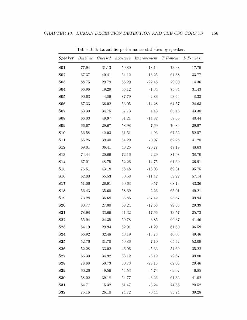
CHAPTER 10. HUMAN DECEPTION DETECTION AND THE CSC CORPUS 156
Table 10.6: Local lie performance statistics by speaker.
Speaker Baseline Guessed Accuracy Improvement T F-meas. L F-meas.
S01 77.94 31.13 59.80 -18.14 73.38 17.79
S02 67.37 40.41 54.12 -13.25 64.38 33.77
S03 88.75 29.79 66.29 -22.46 79.00 14.36
S04 66.96 19.29 65.12 -1.84 75.84 31.43
S05 90.63 4.89 87.79 -2.83 93.46 8.33
S06 67.33 36.02 53.05 -14.28 64.57 24.63
S07 53.30 34.75 57.73 4.43 65.46 43.38
S08 66.03 49.97 51.21 -14.82 58.56 40.44
S09 66.67 29.67 58.98 -7.69 70.86 29.97
S10 56.58 42.03 61.51 4.93 67.52 52.57
S11 55.26 39.40 54.29 -0.97 62.28 41.28
S12 69.01 36.41 48.25 -20.77 47.19 48.63
S13 74.44 20.66 72.16 -2.29 81.98 38.70
S14 67.01 48.75 52.26 -14.75 61.60 36.91
S15 76.51 43.18 58.48 -18.03 69.31 35.75
S16 62.00 55.53 50.58 -11.42 39.22 57.14
S17 51.06 26.91 60.63 9.57 68.16 43.36
S18 56.43 35.60 58.69 2.26 65.01 49.21
S19 73.28 35.68 35.86 -37.42 25.87 39.94
S20 80.77 27.00 68.24 -12.53 79.35 29.39
S21 78.98 33.66 61.32 -17.66 73.57 25.73
S22 55.94 24.35 59.78 3.85 69.37 41.46
S23 54.19 29.94 52.91 -1.29 61.60 36.59
S24 66.92 32.48 48.19 -18.73 46.03 49.46
S25 52.76 31.70 59.86 7.10 65.42 52.09
S26 52.28 33.02 46.96 -5.33 54.69 35.22
S27 66.30 34.92 63.12 -3.19 72.87 39.80
S28 78.88 50.73 50.73 -28.15 62.03 29.46
S29 60.26 9.56 54.53 -5.73 69.92 6.85
S30 58.02 39.18 54.77 -3.26 61.32 41.02
S31 64.71 15.32 61.47 -3.24 74.56 20.52
S32 75.16 26.10 74.72 -0.44 83.74 39.28
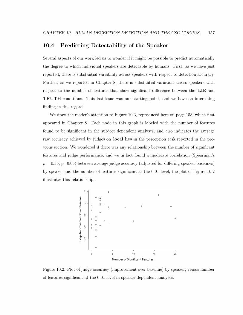
CHAPTER 10. HUMAN DECEPTION DETECTION AND THE CSC CORPUS 157
10.4 Predicting Detectability of the Speaker
Several aspects of our work led us to wonder if it might be possible to predict automatically
the degree to which individual speakers are detectable by humans. First, as we have just
reported, there is substantial variability across speakers with respect to detection accuracy.
Further, as we reported in Chapter 8, there is substantial variation across speakers with
respect to the number of features that show significant difference between the LIE and
TRUTH conditions. This last issue was our starting point, and we have an interesting
finding in this regard.
We draw the reader’s attention to Figure 10.3, reproduced here on page 158, which first
appeared in Chapter 8. Each node in this graph is labeled with the number of features
found to be significant in the subject dependent analyses, and also indicates the average
raw accuracy achieved by judges on local lies in the perception task reported in the pre-
vious section. We wondered if there was any relationship between the number of significant
features and judge performance, and we in fact found a moderate correlation (Spearman’s
ρ = 0.35, p=0.05) between average judge accuracy (adjusted for differing speaker baselines)
by speaker and the number of features significant at the 0.01 level; the plot of Figure 10.2
illustrates this relationship.
Figure 10.2: Plot of judge accuracy (improvement over baseline) by speaker, versus number
of features significant at the 0.01 level in speaker-dependent analyses.
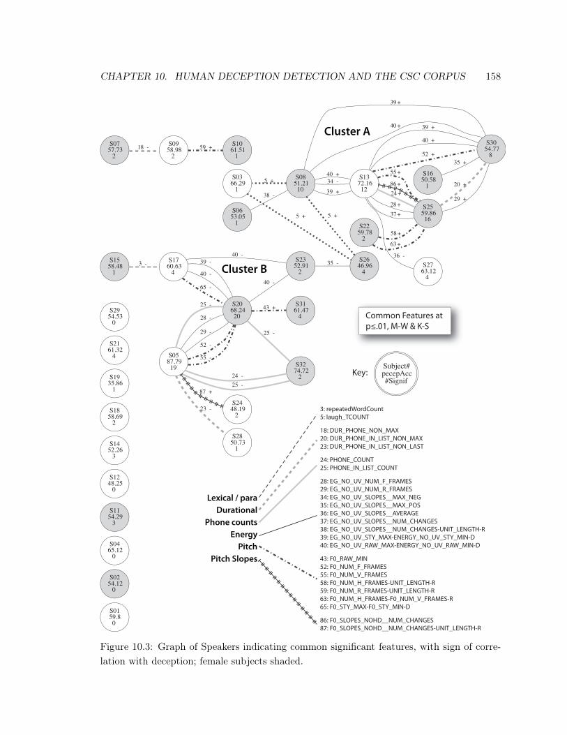
CHAPTER 10. HUMAN DECEPTION DETECTION AND THE CSC CORPUS 158
Lexical / para
Durational
Phone counts
Energy
Pitch
Pitch Slopes
Cluster A
Cluster B
Figure 10.3: Graph of Speakers indicating common significant features, with sign of corre-
lation with deception; female subjects shaded.
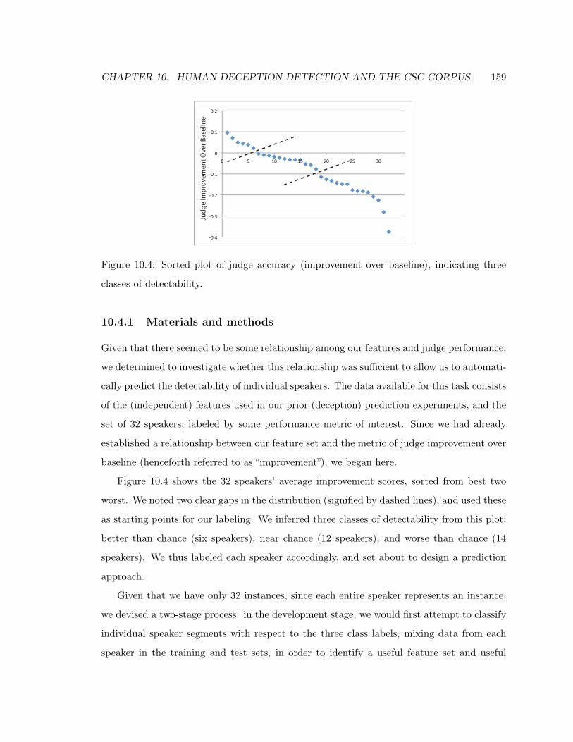
CHAPTER 10. HUMAN DECEPTION DETECTION AND THE CSC CORPUS 159
Figure 10.4: Sorted plot of judge accuracy (improvement over baseline), indicating three
classes of detectability.
10.4.1 Materials and methods
Given that there seemed to be some relationship among our features and judge performance,
we determined to investigate whether this relationship was sufficient to allow us to automati-
cally predict the detectability of individual speakers. The data available for this task consists
of the (independent) features used in our prior (deception) prediction experiments, and the
set of 32 speakers, labeled by some performance metric of interest. Since we had already
established a relationship between our feature set and the metric of judge improvement over
baseline (henceforth referred to as “improvement”), we began here.
Figure 10.4 shows the 32 speakers’ average improvement scores, sorted from best two
worst. We noted two clear gaps in the distribution (signified by dashed lines), and used these
as starting points for our labeling. We inferred three classes of detectability from this plot:
better than chance (six speakers), near chance (12 speakers), and worse than chance (14
speakers). We thus labeled each speaker accordingly, and set about to design a prediction
approach.
Given that we have only 32 instances, since each entire speaker represents an instance,
we devised a two-stage process: in the development stage, we would first attempt to classify
individual speaker segments with respect to the three class labels, mixing data from each
speaker in the training and test sets, in order to identify a useful feature set and useful

CHAPTER 10. HUMAN DECEPTION DETECTION AND THE CSC CORPUS 160
algorithms. In the testing stage, we would treat each speaker as a discrete unit, whereby
no data from a speaker that appeared in the test set would appear in the training set. In
practice, this approach took the form of leave one (speaker) out cross-validation, performed
for each speaker, since we were otherwise hampered by the shortage of data.
The final aspect of this approach entails the question of how to move from segment-level
predictions to classification of the entire speaker. We devised two methods for doing so:
1. Classify each segment for a speaker, then predict the label corresponding to that of
the majority of segments (or possibly applying a threshold to account for the uneven
data distribution, see below).
2. Aggregate the probabilities emitted from the classification algorithm by mean and
standard deviation for each class, then predict class membership of the speaker using
an SVM (this method was not fruitful).
We applied this approach to classifying subjects with respect to the three classes indi-
cated in Figure 10.4, and to two subsets of these classes (see Section 10.4.3).
10.4.2 Three-class prediction
The attempt to classify speakers with respect to all three classes of detectability was ulti-
mately unsuccessful. This approach seemed promising in the development stage, where we
achieved accuracy percentages (classifying individual segments belonging to the speakers)
in the mid-90s, using a feature-selected (Chi-squared ranking) data set of approximately
twenty features with bagging, boosting, and Weka’s implementation of c4.5. However, we
were unable to perform much better than chance at classifying discrete speakers in the testing
stage (and we were particularly hampered by the inability to accurately classify the speakers
in the better-than-chance category), using either the label predicted for the majority of a
given speaker’s segments or SVM classification of the aggregate prediction probabilities, as
described above.

CHAPTER 10. HUMAN DECEPTION DETECTION AND THE CSC CORPUS 161
Figure 10.5: Sorted plot of judge accuracy (improvement over baseline) by speaker, relabeled
for two classes of detectability.
Figure 10.6: Sorted plot of judge accuracy (improvement over baseline), subset of speakers
with two classes of detectability.
10.4.3 Two-class prediction
We next set about to simplify the prediction task, splitting the data into two classes, as
demonstrated in Figure 10.5. In this labeling, the better-than-chance class remains un-
changed, while all speakers on whom judges performed worse than chance are grouped into
one class. We obtained similarly disappointing results at this task, again performing in the
mid-90s in the development stage, but failing to perform better than chance at the testing
stage, again hampered in particular by an inability to classify the better-than-chance class.
Finally, we reframed the task, again as a two-class problem, but this time attempting to

CHAPTER 10. HUMAN DECEPTION DETECTION AND THE CSC CORPUS 162
classify only a subset of speakers, removing those on whom the judges performed near to,
but worse than, chance (i.e. with improvement score S, with 0 > S > −0.1). This labeling
of speakers is illustrated in Figure 10.6.
In this subset of the data, we attempt to differentiate the six speakers who were detected
with better-than-chance accuracy by the judges (labeled good) from the 14 poorly-detected
speakers (labeled poor). In the development stage, we applied feature selection using two
Weka-implemented schemes, Chi-squared ranking and a greedy selection algorithm. The two
feature sets thus selected are displayed in Table 10.8 on page 165. In our prior experiments,
we had determined that c4.5 consistently achieved the best performance at this task, so
we focused our efforts on this classifier. Using c4.5 (implemented by Weka as J48) with
10-fold cross-validation, we achieved a classification accuracy of 92.34% using the 24-feature
set, and an accuracy of 93.21% using the 20-feature set both versus a baseline of 62.17%.
Again, this represents performance in the development stage, where we attempt to classify
individual segments — with segments from each speaker included in both the training and
test sets — in order to ballpark our performance.
In the testing phase, we applied c4.5 to both data sets using leave-one-speaker-out cross-
validation, and additionally applied bagging and boosting in both cases. Finally, we exam-
ined the classification outcomes and found that (presumably as a consequence of the class
imbalance in our data set, 6 good speakers versus 14 poor speakers) applying a threshold
of 36% (meaning that we classified as good any subject at least 36% of whose segments
were classified good, we achieved substantial improvement (2 speakers) with respect to the
minority class, while only suffering one additional mis-classification of the majority class.
Table 10.7 displays the classification results of the testing stage, and Figure 10.7 visualizes
the hits and misses for the two best learners.
10.4.4 Discussion
An examination of the two feature sets reveals a preponderance of pitch and energy features,
particularly those using normalization schemes also employed in speaker recognition; this is
not a surprise, since this task is indeed one that seeks to differentiate individual speakers,
albeit classifying them in terms of a common type of behavior rather than as individuals.

CHAPTER 10. HUMAN DECEPTION DETECTION AND THE CSC CORPUS 163
Table 10.7: Detectability classification performance statistics.
Features/Learner Chance
Chi-sq./c4.5
Chi-sq./c4.5 / B&B
Greedy/c4.5
Greedy/c4.5 / B&B
Greedy/c4.5/B&BThreshold
Accuracy 70% 65% 65% 75% 80% 85%
Hits – Good 0 1 1 3 3 5
Hits – Poor 14 12 12 12 13 12
The best-performing feature set also contains a number of lexical and discourse features,
including cue phrases and unintelligible and mispronounced word counts, and these features
are familiar to us, having been significant in our subject dependent analyses. The tree
constructed by c4.5 makes heavy use of energy features as top-level features, while seeming
to employ the lexical features at the leaves; this would suggest that broad categories of
speakers are differentiated by the energy features. There is to our knowledge no precedent
in the literature for the automatic prediction of detectability of speakers, so we are unable
to draw parallels to existing work.
There is one aspect of the literature that does have some bearing on this task. In exam-
ining factors that predicted performance, we expected, based on common assumptions in the
Figure 10.7: Hits and misses for best detectability classification algorithms and feature set.
Both cases employ c4.5 with bagging and boosting; best learner uses 36% threshold for
predicting GOOD. Misses indicated with X.

CHAPTER 10. HUMAN DECEPTION DETECTION AND THE CSC CORPUS 164
literature (e.g. (Ekman, 2001)), that good liars would tell the truth most of the time; more
rigorously, that the density of local lies per global lie would influence human accuracy at
predicting global lies . It is commonly held that successful liars tell the truth most of the
time, and the CSC paradigm particularly lends itself to this sort of comparison. Our data
did not, in fact, support this assumption: the density of local lies in global lies did not
have a significant effect on judge performance. This suggests that this assumption might
merit further consideration.
Although the final performance on the task as ultimately conceived is fairly good, we
had of course hoped to be able to classify the entire set of subjects. Our results do, however,
suggest to us that there are some readily detectable differences in behavior between speakers
who are somewhat easier for human judges to catch in a lie and those who are very difficult
to catch. Such differences are not automatically discernible, however (at least using our
current feature set) for speakers whose detectability lies somewhere in the middle. There
is some incentive to continue research in this vein, as it could be useful on at least two
levels. First, and most obviously, if speakers’ degree of detectability could be discerned with
confidence independently of any data entailing ground truth, interview methods by human
investigators might be adjusted accordingly. Second, if predicted with high confidence,
detectability ratings of individual speakers might be integrated into performance measures
for deception detection tasks, weighting success or failure on various subjects based on their
relative (predicted) detectability by humans (Owen Rambow, personal communication, July
17, 2008). As a final note, we find it intriguing that there seems to be a relationship between
the number of features that show significant differences between TRUTH and LIE for
individual subjects and the performance of human judges at detecting their deceptions.
Although we hesitate to draw strong inferences from the moderate correlation we reported,
one possible explanation is that human judges are detecting behaviors that correlate with,
or are captured by, some elements of our feature set.
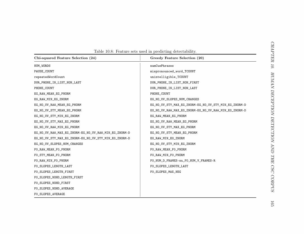
CH
AP
TE
R10.
HU
MA
ND
EC
EP
TIO
ND
ET
EC
TIO
NA
ND
TH
EC
SC
CO
RP
US
165
Table 10.8: Feature sets used in predicting detectability.
Chi-squared Feature Selection (24) Greedy Feature Selection (20)
NUM_WORDS numCuePhrases
PAUSE_COUNT mispronounced_word_TCOUNT
repeatedWordCount unintelligible_TCOUNT
DUR_PHONE_IN_LIST_NON_LAST DUR_PHONE_IN_LIST_NON_FIRST
PHONE_COUNT DUR_PHONE_IN_LIST_NON_LAST
EG_RAW_MEAN_EG_PNORM PHONE_COUNT
EG_RAW_MIN_EG_ZNORM EG_NO_UV_SLOPES_NUM_CHANGES
EG_NO_UV_RAW_MEAN_EG_PNORM EG_NO_UV_STY_MAX_EG_ZNORM-EG_NO_UV_STY_MIN_EG_ZNORM-D
EG_NO_UV_STY_MEAN_EG_PNORM EG_NO_UV_RAW_MAX_EG_ZNORM-EG_NO_UV_RAW_MIN_EG_ZNORM-D
EG_NO_UV_STY_MIN_EG_ZNORM EG_RAW_MEAN_EG_PNORM
EG_NO_UV_STY_MAX_EG_PNORM EG_NO_UV_RAW_MEAN_EG_PNORM
EG_NO_UV_RAW_MIN_EG_PNORM EG_NO_UV_STY_MAX_EG_PNORM
EG_NO_UV_RAW_MAX_EG_ZNORM-EG_NO_UV_RAW_MIN_EG_ZNORM-D EG_NO_UV_STY_MEAN_EG_PNORM
EG_NO_UV_STY_MAX_EG_ZNORM-EG_NO_UV_STY_MIN_EG_ZNORM-D EG_RAW_MIN_EG_ZNORM
EG_NO_UV_SLOPES_NUM_CHANGES EG_NO_UV_STY_MIN_EG_ZNORM
F0_RAW_MEAN_F0_PNORM F0_RAW_MEAN_F0_PNORM
F0_STY_MEAN_F0_PNORM F0_RAW_MIN_F0_PNORM
F0_RAW_MIN_F0_PNORM F0_NUM_D_FRAMES-wu_F0_NUM_V_FRAMES-R
F0_SLOPES_LENGTH_LAST F0_SLOPES_LENGTH_LAST
F0_SLOPES_LENGTH_FIRST F0_SLOPES_MAX_NEG
F0_SLOPES_NOHD_LENGTH_FIRST
F0_SLOPES_NOHD_FIRST
F0_SLOPES_NOHD_AVERAGE
F0_SLOPES_AVERAGE

CHAPTER 10. HUMAN DECEPTION DETECTION AND THE CSC CORPUS 166
10.5 The Personality of the Hearer: Effects on Performance
An important finding of this study is a set of strong relationships among three personality
factors (measured via the NEO-FFI inventory of Costa and McCrae’s (1992, 2002) widely
used five factor model of personality) and performance at deception detection. As our ideas
about individual differences in deceivers continued to form, we became interested in the
possibility of such differences among hearers, particularly those relating to personality. There
is a relative paucity of studies that address this particular question. Aamodt and Custer
(2006) found that only the personality trait of self-monitoring approached meta-analytic
significance as a cue to lie-detection ability, and they lament the shortage of relevant studies
(a total of 12, versus e.g. 193 that address the abilities of professionals), suggesting that
this is a fertile area for further research.
10.5.1 Materials and methods
In order to examine individual differences among judges, prior to the perception task,
judges completed the NEO-FFI form, measuring the Costa & McCrae five-factor personality
model, a widely used personality inventory for nonclinical populations (Costa & McCrae,
1992; Costa & McCrae, 2002). The five factor model, known also as the “Big Five”, is a con-
struct of personality psychology that posits five persistent personality traits: Neuroticism,
Extraversion, Openness to Experience, Agreeableness, and Conscientiousness. This model
represents a lexical approach to trait psychology, and the five dimensions were derived via
factor analysis of lists of adjectives that are employed by individuals in describing themselves
and others (Costa & McCrae, 1992):
Neuroticism contrasts emotional stability with maladjustment; the contrasts captured
include those between individuals prone to worry versus calm, emotional versus un-
emotional behavior, and hardiness versus vulnerability.
Extraversion captures an individual’s proclivity for interpersonal interactions, and de-
scribes variation in sociability. This factor reflects contrasts between those who are
reserved and outgoing, quiet and talkative, and active and retiring.

CHAPTER 10. HUMAN DECEPTION DETECTION AND THE CSC CORPUS 167
Openness to Experience or “Openness” captures imagination, aesthetic sensitivity, and
intellectual curiosity. Those who score low on this dimension prefer the familiar and
tend to behave more conventionally. Openness is distinct from intelligence, which
Costa and McCrae hold to be outside the realm of personality proper, yet it is “related
to aspects of intelligence, such as divergent thinking, that contribute to creativity”
(Costa & McCrae, 1992). People high in Openness are “willing to entertain novel
ideas and unconventional values” (Costa & McCrae, 1992). Openness is of particular
interest in deception detection since it addresses the degree to which a listener might
be willing to set aside preconceptions and take in all aspects of an immediate situation,
which in the case of our experiment comprises the behavior of the speaker in the given
context. It also seems reasonable to expect that a listener who scores high in Openness
would be more able to defer judgement (specifically in terms of the deceptiveness of
the speaker) until s/he has observed all available information rather than making facile
conclusions, a trait surely of use in this context.
Agreeableness is a measure of a class of interpersonal tendencies, and its meaning is
slightly unintuitive when compared to the usage of agreeableness in common parlance.
At its base, Agreeableness is a measure of an indivdual’s fundamental altruism, and
individuals high in Agreeableness are sympathetic to others and expect that others feel
similarly. From the standpoint of deception detection, Agreeableness is of particular
interest in that it correlates with the degree to which an individual is empathic (Nettle,
2007), and a hearer’s sensitivity to a speaker’s subjective state is likely of great value
in deception detection given the strong affective component of deception cues.
Conscientiousness addresses individual differences in the realm of self-control. This refers
to the ability to control impulses, but also to more active processes such as planning
and carrying out tasks (Costa & McCrae, 1992). Contrasts measured by this dimension
include those between determination, organization, and self-discipline in high-scorers
and laxness, disorganization, and carelessness in low-scorers.
Judges completed the NEO-FFI form prior to being told that the experiment entailed a
deception detection task; this approach was employed in order to avoid priming the judges’

CHAPTER 10. HUMAN DECEPTION DETECTION AND THE CSC CORPUS 168
responses to the personality inventory. The completed NEO-FFI forms were subsequently
scored by a licensed clinical psychologist who collaborated on the project.
We found a number of significant effects for personality variables and deception detec-
tion performance and related behaviors. We report both correlation measures — Pearson’s
correlation coefficient — and multiple-linear regression models obtained on our data. Stan-
dard assumptions with respect to normality, variance, and absence of covariance among the
independent variables were met in these models. The models were subjected to standard di-
agnostic measures (DFFITS, DFBETAS, Studentized residuals, Cook’s D) (Neter, Kutner,
Nachtsheim & Wasserman, 1996). In each model one or two potentially influential cases
were identified, so we applied robust regression techniques (Neter, Kutner, Nachtsheim &
Wasserman, 1996): least median of squares, least trimmed squares, and simply removing
the suspect points. In all cases, results were comparable, and in some cases better, than the
ordinary least squares models reported here. Although our sample represents 32 judges, we
feel the size is mitigated by the extremely small p-value for the F-statistic of the R2 values,
except in the case of the model of proportion of lies guessed, where we warn against making
strong inferences.
10.5.2 Results
We tested the correlation of each of the five personality factors against the measures of per-
formance computed for both global and local lies : accuracy, improvement over baseline,
F-measure for both TRUTH and LIE , and percentage of items labeled LIE by the judge
(regardless of accuracy; this is in a sense a measure of a judge’s truth/lie bias, or assumed
priors). Correlations significant at the 0.05 level or better were found for three personal-
ity factors: Openness, Agreeableness, and Neuroticism. These relationships exist only for
performance measures with respect to global lies except for the case of improvement over
baseline, which shows moderately significant correlation with one personality factor (Agree-
ableness) at the local lie level as well. These results are reported in Table 10.9. Table
10.10 shows regression models constructed on the factors and measures shown in Table 10.9.
We draw the reader’s attention to the particularly strong predictive power of the models
using the factor Openness, i.e. those for accuracy, improvement over baseline (with respect

CHAPTER 10. HUMAN DECEPTION DETECTION AND THE CSC CORPUS 169
Table 10.9: Correlations between personality factors and various measures of judge perfor-
mance. Performance measures relate to global lie except where otherwise noted.
Factor Measure Pearson’s p-value
Neuroticism Proportion of segments judged LIE -0.44 0.012
Openness Accuracy 0.51 0.003
Agreeableness 0.41 0.021
Openness Improvement over baseline 0.47 0.007
Agreeableness 0.38 0.032
Neuroticism F-measure for TRUTH 0.37 0.035
Agreeableness 0.41 0.019
Openness F-measure for LIE 0.52 0.003
Agreeableness Improvement over baseline (Local) 0.35 0.047
to global lies) and F-measure for LIE. Although the regression coefficients are small in
absolute terms, it is important to note that the NEO-FFI factors are expressed in whole
number percentile scores, effectively ranging from 25 to 75, while performance measures are
expressed as decimal fractions. Thus, a regression coefficient of 0.01 (as in the model of F-
measure for LIE with respect to Openness) represents a high correlation between Openness
and F-measure. To illustrate this, Figure 10.8 demonstrates the fit of the regression line
for three of the most interesting models; the slope of the line in all three cases conveys our
point with respect to the degree of correlation.
It is not surprising to find significant effects for Openness with respect to detection
performance. This factor measures the degree to which an individual is available to new
experience and able to adjust viewpoints, and as we described earlier, it correlates with
aspects of intelligence related to creativity (Costa & McCrae, 1992). We believe that this
factor enhances the ability of the judge to base decisions on the available data rather than
on preconceptions, and thus contributes to judge performance in the manner reflected in
the models for accuracy, improvement over baseline (global lie) and F-measure for LIE.
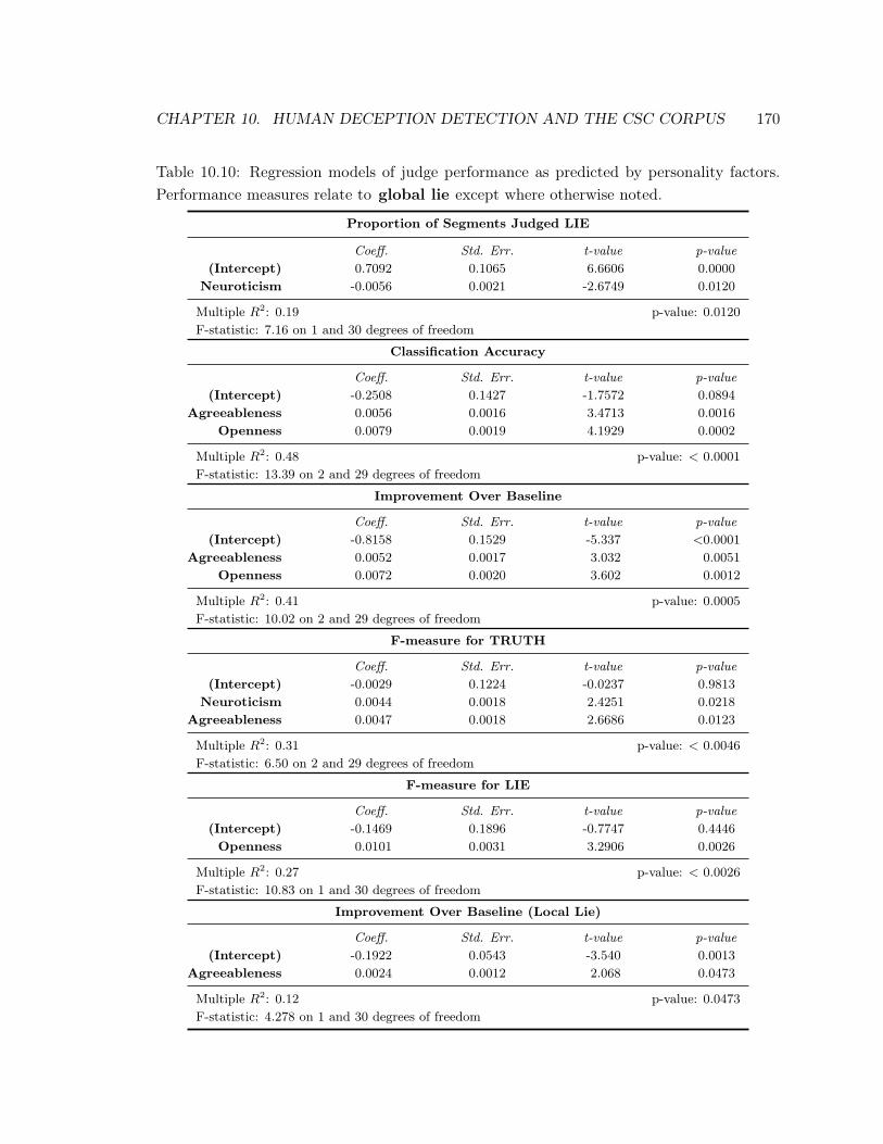
CHAPTER 10. HUMAN DECEPTION DETECTION AND THE CSC CORPUS 170
Table 10.10: Regression models of judge performance as predicted by personality factors.
Performance measures relate to global lie except where otherwise noted.
Proportion of Segments Judged LIE
Coeff. Std. Err. t-value p-value
(Intercept) 0.7092 0.1065 6.6606 0.0000
Neuroticism -0.0056 0.0021 -2.6749 0.0120
Multiple R2: 0.19 p-value: 0.0120
F-statistic: 7.16 on 1 and 30 degrees of freedom
Classification Accuracy
Coeff. Std. Err. t-value p-value
(Intercept) -0.2508 0.1427 -1.7572 0.0894
Agreeableness 0.0056 0.0016 3.4713 0.0016
Openness 0.0079 0.0019 4.1929 0.0002
Multiple R2: 0.48 p-value: < 0.0001
F-statistic: 13.39 on 2 and 29 degrees of freedom
Improvement Over Baseline
Coeff. Std. Err. t-value p-value
(Intercept) -0.8158 0.1529 -5.337 <0.0001
Agreeableness 0.0052 0.0017 3.032 0.0051
Openness 0.0072 0.0020 3.602 0.0012
Multiple R2: 0.41 p-value: 0.0005
F-statistic: 10.02 on 2 and 29 degrees of freedom
F-measure for TRUTH
Coeff. Std. Err. t-value p-value
(Intercept) -0.0029 0.1224 -0.0237 0.9813
Neuroticism 0.0044 0.0018 2.4251 0.0218
Agreeableness 0.0047 0.0018 2.6686 0.0123
Multiple R2: 0.31 p-value: < 0.0046
F-statistic: 6.50 on 2 and 29 degrees of freedom
F-measure for LIE
Coeff. Std. Err. t-value p-value
(Intercept) -0.1469 0.1896 -0.7747 0.4446
Openness 0.0101 0.0031 3.2906 0.0026
Multiple R2: 0.27 p-value: < 0.0026
F-statistic: 10.83 on 1 and 30 degrees of freedom
Improvement Over Baseline (Local Lie)
Coeff. Std. Err. t-value p-value
(Intercept) -0.1922 0.0543 -3.540 0.0013
Agreeableness 0.0024 0.0012 2.068 0.0473
Multiple R2: 0.12 p-value: 0.0473
F-statistic: 4.278 on 1 and 30 degrees of freedom
CHAPTER 10. HUMAN DECEPTION DETECTION AND THE CSC CORPUS 171
There is support for this determination in the literature, as well. We have described earlier
in this chapter how the confidence borne of experience does not contribute to police officers’
deception detection skills, and this may be interpreted as an over-reliance on preconceptions
in making judgments. Conversely, the subject who scores high in openness is willing to
adjust or set aside preconceptions when confronted with new information. Ekman (2001)
describes a number of conclusions he has reached during his long investigation of deception
detection. Among these is his confidence that success at detecting lies is maximized when
“the interviewer is truly open-minded, and does not jump to conclusions quickly” (Ekman,
2001). This clearly describes the subject who is high in openness, and essentially predicts
the findings we report here with respect to this factor.
Individuals who score high in Agreeableness tend to be “compassionate, good natured,
and eager to cooperate and avoid conflict” (Costa & McCrae, 1992). Initially, then, it
seems unintuitive that Agreeableness should be a predictor of success at deception detec-
tion. However, an extremely high score in Agreeableness is associated with a pathology
known as dependent personality disorder (Costa & McCrae, 1992). This pathology manifests
itself in extreme attention to the opinions and affective state of others (American Psychi-
atric Association, 2000); likewise, the qualities of compassion and eagerness to cooperate
entail sensitivity to affect. We believe that it is this sensitivity that enhances the judge’s
ability to perceive cues to deception. This is consistent with the (albeit weak) evidence
we described earlier (Aamodt & Custer, 2006) that suggests that people who are highly
self-monitoring (individuals who are particularly attuned to the impressions and attitudes
of others) do well at the deception detection task. In a tangential way, Ekman (2001) makes
a similar prediction. He predicts greater success on the part of “the interviewer [who] knows
how to encourage the interviewee to tell his story” (Ekman, 2001). Although the aspect of
encouragement is not at play here since the judges are listening to recorded interviews, this
description clearly suggests that empathy is of value to the interviewer, and as we noted
earlier, Agreeableness is a correlate of empathy.

CH
AP
TE
R10.
HU
MA
ND
EC
EP
TIO
ND
ET
EC
TIO
NA
ND
TH
EC
SC
CO
RP
US
172
Figure 10.8: Plots of fitted lines for regression models with respect to global lie performance measures. Lines represent a linear
combination of coefficients where more than one independent variable is represented.

CHAPTER 10. HUMAN DECEPTION DETECTION AND THE CSC CORPUS 173
There is an interesting negative correlation between Neuroticism and the proportion of
sections labeled LIE by judges. We wondered whether this was a function of behavior at the
time of labeling, or of the judges’ prior expectations that a speaker would lie. We found, in
fact, a negative correlation (Pearson’s cor: -0.39, p=0.0277) between Neuroticism and judges’
pre-test report of their expectation of the frequency with which people lie in general.4 This
correlation clearly merits further investigation. We speculate that Neuroticism may entail
an inflated need to believe that people are generally truthful, since the neurotic individual
suffers more than others when faced with upsetting thoughts or negative perceptions (Costa
& McCrae, 2002). In addition there is a positive correlation between Neuroticism and F-
measure for TRUTH; this is fairly intuitive, since a bias toward guessing TRUTH may
well impact a measure that can favor prediction of TRUTH.
As a final illustration of the effects we have described here, we present four individual
subjects and the relationships between the factors and performance measures we have de-
scribed. Although it is of course ill-advised to draw strong inferences from any individual
case, the best and worst cases in the present data (with respect to the performance mea-
sures in question) reflect very clearly the types of relationships modeled among Openness,
Agreeableness, and the various performance measures. Figure 10.9 represents the person-
ality scores and selected performance measures of four judges, all with respect to global
lie . Judge 32 performed best out of all judges in terms of both accuracy and F-measure for
LIE ; this judge also received the highest possible score on Openness. Judge 12 performed
second best and third best of all subjects on accuracy and F-measure for LIE , respectively,
and likewise scored very high on Agreeableness. On the other end of the performance spec-
trum, Judge 9 scored worst on both accuracy (tie) and F-measure for LIE , and received
an extremely low score on Openness. Finally, Judge 3 performed worst (tie) with respect
to accuracy and second worst with respect to F-measure for LIE , and likewise received the
lowest possible score for Agreeableness.
After examining the bar charts of Figure 10.9, we encourage the reader to reexamine the
plots of Figure 10.8 in order to verify that while these judges represent the maximum and
minimum cases with respect to performance and personality scores, there are no obvious
4No other correlations between personality factors and judges’ priors were found.

CH
AP
TE
R10.
HU
MA
ND
EC
EP
TIO
ND
ET
EC
TIO
NA
ND
TH
EC
SC
CO
RP
US
174
Figure 10.9: Bar charts of personality scores for best two and worst two performing subjects with respect to global lie performance
measures. Personality scores reflect Neuroticism, Extraversion, Openness to Experience, Agreeableness, and Conscientiousness.

CHAPTER 10. HUMAN DECEPTION DETECTION AND THE CSC CORPUS 175
extreme outliers; rather these cases seem to be consistent with the general trends of the data.
Again, we warn against making strong inferences here, but we offer these specific cases since
they represent a fairly principled selection criterion (the best and worst cases with respect to
the performance measures) and vividly illustrate the relationships discovered in this study.
10.6 Conclusions
We have examined the performance of humans in distinguishing truth from lie in the CSC
corpus of deceptive speech. Our findings have important implications for research in ma-
chine detection of deceptive speech and for the understanding of human performance on the
deception task. One of the best-documented claims in the literature is that the deception
detection task is extremely difficult for humans (DePaulo, Lindsay, Malone, Muhlenbruck,
Charlton & Cooper, 2003; Aamodt & Custer, 2006), particularly when speech is the only
channel of communication available. In the present study, judges perform on average worse
than chance. We thus note the success of machine learning methods in predicting deception
in the CSC corpus, since results exceed both chance and human performance.
There is also considerable evidence that individual differences must be taken into account
in deception detection, whether by humans or machines (O’Sullivan & Ekman, 2004). This
appears to be supported by the variability of our judges’ success in detecting individual
speakers in the present study, and supports our idea that future efforts must model such
individual differences in automatic deception detection.
We have presented some novel results for the task of predicting the detectability of
individual speakers, and we believe this warrants further investigation, both in terms of our
finding that the number of significant features in our subject-dependent analysis correlates
with human detectability, and that human detectability is to some degree predictable.
From the point of view of improving human efforts at detection, we are intrigued by
evidence that personality variables have an impact on a judge’s success. This finding may
help to identify good human detectors of deception and point toward ways individuals can
be trained to become better detectors. Further, knowledge of what kinds of people are good
detectors may lead to better identification of reliable objective cues to deception in speech.

PART V. 176
Part V
Conclusions

PART V. 177
Chapter 11
Conclusions
We have presented in this dissertation a series of analyses and experiments that address
deceptive speech from the perspective of spoken language processing. In Section I we de-
scribed the motivations for our approach, and introduced a new corpus of deceptive speech,
the CSC Corpus.
In Section II we undertook a variety of analyses and classification experiments using
features novel to the deception detection domain, and showed a number interesting effects for
deception with respect to these features. We also showed that it is possible to automatically
classify truthful and deceptive speech in the CSC Corpus with an accuracy better than
chance and considerably better than human listeners.
In Section III we undertook a variety of subject-dependent and group-dependent analyses
and experiments. We showed evidence of individual differences in deceptive behaviors, and
described distinct speaking styles that seem to be employed by different groups of speakers in
deceptive interactions. We applied our machine learning techniques to subgroups of speakers
that were identified using a variety of principled methods, and showed that classification
results for certain groups exceeded results for the aggregate data.
In Section IV we reported a perception study that engaged human hearers to attempt
to detect deception in the CSC Corpus. These hearers performed on average quite poorly,
achieving worse than chance accuracy on both local and global lies. We also reported
novel findings on the relationship of personality to the ability to detect deception in speech.

PART V. CONCLUSIONS 178
11.1 Summary of Findings
11.1.1 Statistical Analyses
In Chapter 4 we described corpus-wide analyses of three broad classes of features with
respect to the local lie condition: binary lexical, paralinguistic and discourse features;
lexical, paralinguistic and discourse features that are expressed numerically; and numerical
acoustic and prosodic features.
11.1.1.1 Binary lexical features
Chi-squared analysis (Section 4.2) showed that eight binary features vary significantly be-
tween the TRUTH and LIE conditions in the aggregate data. The use of third person
pronouns, cue phrases, positive emotion words, the n’t contraction, and not increased in
the LIE condition. The use of filled pauses, questions, and of a question in response to a
question all decreased in the LIE condition.
Our findings vary with respect to their consistency with existing literature. The use
of third person pronouns increases with deception, consistent with the findings of DePaulo
et al. (2003) and Hancock (2004), but in contrast to Newman et al. (2003), who report
the opposite. Our findings with respect to cue phrases, such as actually, basically, also
and ok, are consistent with the literature (Adams, 1996) and practitioner claims (Reid &
Associates, 2000), which suggest that more cue phrases should appear in deceptive speech.
Burgoon et al. (2003) report a higher incidence of positive emotion words in deception,
and we found the same. Our findings with respect to the two negative constructs not an
n’t are also consistent with the literature (Adams & Jarvis, 2006; DePaulo et al., 2003).
DePaulo et al. (2003) report ambiguous findings with respect to filled pauses as a cue.
Our findings regarding questions contradict existing literature (DePaulo et al., 2003), which
suggests that question asking represents avoidance and should thus correlate with deception;
we offer the alternative possibility that truthful subjects ask questions in order to promote
communication.
PART V. CONCLUSIONS 179
11.1.1.2 Numerical features
We reported in Section 4.3 our analyses of numerical features with respect to the local
lie condition. Among these features, counts of filled pauses are significant, again appear-
ing more often in truthful speech. The repetition of words occurs more frequently in the
TRUTH condition. DePaulo (2003) found likewise, though Vrij (2008) found repetition to
be inconclusive.
Four silent pause features show significant effects, and combine to capture an interesting
phenomenon. As we described in Chapter 4, while two features — the total duration of
silent pauses in a segment and the maximum duration of a silent pause for the segment
— correlate with TRUTH, two features capturing the length of the pauses immediately
preceding and following a given segment correlate with LIE. This suggests that, while the
truth teller exhibits pausing during a segment, the deceiver inhibits such segment-internal
pausing. In contrast, pauses of increased length occur on either side of deceptive segments,
possibly signaling cognitive load.1 The literature is ambiguous regarding silent pauses and
deception. The ratio of the number of voiced frames to segment length also showed an
increase in the LIE condition and may reflect increased speaking rate or decreased internal
pausing.
Two durational features (measuring phone duration) are significant, signaling shorter
duration in deceptive speech. This is inconsistent with Hall’s (1986) examination of syllabic
duration of (one word) Control Question Test polygraph responses, which found increased
duration in deceptive answers.
Three energy slope features are significant in an interesting combination: while values for
the first and last slopes of a segment are greater in deception, the average energy slopes of
a segment correlate negatively with deception. This possibly signals a more abrupt “attack”
and “release” in deceptive segments, with, on average, a decline in energy over the course of
the segment. Smaller average energy slopes seem to be consistent with one study (Sayenga,
1983) but the literature is otherwise inconclusive around energy or amplitude.
A number of features measuring pitch halving show positive correlation with deception.
1Most subject turns contain multiple SUs, causing turn-internal pauses to dominate these features so
that the pause preceeding the SU is not generally a proxy for response latency. See Section 4.3.1 for details.

PART V. CONCLUSIONS 180
Halving can occur in the presence of vocal fry or diplophonia (Johnson, 2003), possibly as a
result of “forced” or overly energetic speech production. Liscombe (2007) showed precedent
for the use of pitch mistracking in the identification of affective state, finding that mistracks
were a helpful cue to the emotion sadness.
Minimum stylized pitch correlates positively with deception, consistent with a large
number of studies (Streeter et al., 1977; Scherer et al., 1985; Hall, 1986; Ekman et al.,
1991) that show a general pitch increase in the deceptive condition. Our other significant
pitch features — generally capturing range and slope — correlate negatively with deception,
suggesting speech that is falling or flat. To our knowledge no existing literature addresses
these more complex prosodic features.
11.1.2 Classification of local lies
We completed a variety of experiments using five different classification algorithms and four
different feature sets to classify local lies with respect to the SU segmentation. Our
best results were obtained using the c4.5 classifier and the Best 39 feature set, a subset of
features obtained using Chi-squared feature selection criteria. With this classifier/feature set
combination we obtained average accuracy of 70.00% vs. a majority class baseline of 59.93%.
Using the binomial model, we established a criterion requiring a difference of 3.3% to ensure
significance at the 0.05 level, which is clearly met by this result. The Best 39 feature set
is enumerated in Table 5.6 on page 67, and includes a subset of subject-dependent, lexical,
paralinguistic, durational, energy, and pitch features; numerical features were normalized
within subject.
Specifically, the set captures behaviors such as pausing, speech disturbances and unin-
telligibility, which seem to address DePaulo et al’s (2003) hypotheses with respect to the
construct of fluency and compelling-ness. It also captures lexical features related to emotion
words (Newman et al., 2003). A number of POS-related features appear, along discourse
features relating to cues phrases or questions, all inspired by practitioners’ intuitions (e.g.
(Reid & Associates, 2000)). Three features capturing change (slope) in energy appear in
this set, as does one feature (F0_SLOPES_NOHDFIRST) capturing pitch slope; we found no
treatment of such features in the literature. As in our statistical analysis, features capturing

PART V. CONCLUSIONS 181
pitch-halving also appear.
In the tree learned for this feature set, subject-dependent features generally appear as
top-level nodes. Lexical features (yes, no, and positive and negative emotion words) predom-
inate on the leaves; exceptions to this tend to be energy slope or durational features. Topic
appears as a mid-level feature, generally in combination with various lexical features. The
model gives the overall impression that subject-dependent features divide segments by types
of speaker, and that the segments are further differentiated by lexical and acoustic/prosodic
features at the leaves.
11.1.3 Classification of global lies
We classified global lies by identifying proxy segments that we termed “critical segments”,
speaker segments that responded directly to the interviewer’s questions regarding the speaker’s
scores on the six topic areas of the pre-test. We also experimented with a larger set that
included responses to the interviewer’s immediate follow-up question. We labeled the two
sets of segments the Critical set and Critical-Plus set, respectively. The data distribu-
tion is skewed in favor of the LIE category, and using the original data with this skewed
distribution, the c4.5 classifier performed only slightly better than chance. Interestingly, we
found that by downsampling the data to an even distribution of LIE and TRUTH, our
best performance improved to 61.9% vs. a 50% chance baseline on the Critical set. It is
of course less than desirable to alter the true distribution of the data, but as will be seen
below, doing so produced a fairly intuitive classifier model. This issue of class distributions
will be addressed further in our concluding remarks.
The rules induced by the classifier for this data are fairly intuitive, and consistent with
previous literature. As we described in Section 6.3.1, the presence of negative or positive
emotion words (Whissel, 1989; Newman et al., 2003) appears prominently in the models,
with positive emotion words often correlating positively with truth. We also find rules based
on features that might relate to the quality of being “compelling” (DePaulo et al., 2003).
Assertive terms as yes or no serve as a cue to deception. Likewise, a specific, direct denial
(e.g. “I did not”) is used in many rules as a cue to truth (Reid & Associates, 2000). Cue
phrases also appear as a cue to deception in the models. Filled pauses appear as a cue to

PART V. CONCLUSIONS 182
truth in many rules produced, as do self-repairs, and both are consistent with the finding
of DePaulo et al. (2003) that liars’ speech exhibits fewer ordinary imperfections. Finally, it
appears that extreme values for energy correlate with deception.
11.1.4 Speaker dependent analyses
We repeated the statistical analyses described in Chapter 4 on a within-speaker basis, con-
sidering differences between the TRUTH and LIE conditions for each speaker using non-
normalized data.
11.1.4.1 Binary features
We provided extensive detail of our analyses of these features in Section 8.2, so we will confine
our comments here primarily to high-level observations. Whereas in the aggregate data,
only 8 of the 25 binary features show significant differences between LIE and TRUTH,
19 features show differences at the 0.05 significance level in the subject dependent analyses.
Interestingly, in almost every case, the direction of correlation with deception demonstrated
by a given feature is evenly distributed across the subjects for which it is significant. For
example, the presence of the pronoun I correlates positively with deception for two subjects
and negatively for two others. This pattern is repeated for most of the 19 significant features.
Subjects vary from 0 to 5 with respect to the number of features that evidence significance.
Likewise, the number of subjects per feature ranges from 0 to 7.
Seventy-five percent (40/53) of the instances of significant binary features (the inter-
section of a given feature with one subject) fall into one or more of three categories:
features reflecting a formal or “careful” speaking style (Biber, 1991) (hasFilledPause,
hasSelfRepair, hasContraction, hasNaposT; features that capture the degree to which
the speaker’s discourse occurs in the first person (hasI and hasWe); and features that ex-
press emotional or semantic valence, or literally have positive or negative semantic value
(hasPositiveEmotionWord, hasNegativeEmotionWord, hasNot, hasNapostT, hasYes,
hasNo, noYesOrNo, isJustYes, isJustNo).

PART V. CONCLUSIONS 183
11.1.4.2 Numeric Features
Again, we provided extensive detail regarding our speaker dependent analyses of numeric
features in Section 8.3; we will highlight here two major findings.
First, there is great variation among subjects with respect to which features are signifi-
cant, and to the direction of correlation of those features. On a higher level, there is likewise
great variation among subjects with respect to the classes of features that are significant;
this is visualized in Figures 8.7 and 8.8 on pages 114 and 115. Those figures indicate 24
instances of significance of our pitch slope features across ten subjects; 28 instances of sig-
nificance of pitch features across 14 subjects; 33 instances of significance of energy features
across 12 subjects, and six instances of significance for our pause features for two subject.
Certain subjects exhibit multiple effects with respect to related features, such as multiple
pitch features, and some subjects overlap or to share categories. It is possible, of course,
that subjects share significant features but differ with respect to direction of correlation,
and we have thus devised a novel approach to inferring similar behaviors among subjects.
Our second major finding follows from this novel approach: using a graph-based cluster-
ing algorithm described and visualized in Section 8.3.2 and in Figure 8.9, we have inferred
two distinct deceptive speaking styles among a majority of our subjects.
One group of ten speakers evidences patterns of features and directions of correlation
that describe speech that is more variable and animated in the deceptive condition. In
particular, two features that capture range of energy in the segment appear repeatedly in
this cluster, as do other features indicating increased or variable energy, such as maximum
positive slope, the number of rising frames, and the number of slope changes; maximum
negative slope appears with negative correlation. The count of laughs appears in this cluster
with positive correlation. Four pitch features — counts of falling and voiced frames, and
two features capturing halved frames — all correlate positively with deception. Together,
these features, given their directions of correlation, describe animated speech, suggesting the
possibility that some liars “oversell” the lie, producing speech that is perhaps intentionally
more engaging in the LIE condition.
A group of nine speakers conversely evidences less animated speech in the deceptive
condition. Specifically, energy features that capture range of energy in the segment appear
PART V. CONCLUSIONS 184
repeatedly and with negative correlation; energy features that capture maximum positive
slope and rising frames are also negatively correlated. Pitch features are also consistent with
less animation or vocal immediacy: minimum pitch is positively correlated with deception,
while falling frames and voiced frames are negatively correlated. Vowel duration is shorter
in the deceptive condition. Repeated word count is negatively correlated for two speakers,
possibly a reflection of more careful speech.
11.1.5 Group dependent classification
In Chapter 9 we reported two sets of experiments that grouped subjects: first by gender
and then by the graph derived clusters described in the previous section. These experiments
yielded mixed results. The group of male subjects appeared to realize the best performance
achieved on the corpus (74.47% accuracy vs. a baseline of 61.24%), using the Best 39 feature
set with c4.5. However, when we combined these results with those for the female subjects
via a weighted average, they were statistically identical to the previous best performance —
70.00% — reported for the aggregate data. Likewise, results using the clustered speakers
did not improve upon results for the aggregate data, either in terms of performance achieved
for the individual clusters or the weighted average over both. We attribute this performance
primarily to limitations of the univariate analysis used in generating the clusters, since this
approach could not exploit the complex dependencies that can be captured by learning
algorithms such as c4.5.
11.1.6 Human performance at classifying the CSC Corpus
In Chapter 10 we reported a perception study in which human subjects were recruited to
attempt to detect deception in the corpus on both the local and global lie levels. Their
performance was quite poor: on average they scored worse than the majority class baseline
at both tasks. These results place our machine learning results in a fairly positive light,
since our classifiers substantially exceeded human performance in both cases.
We also reported in Chapter 10 a number of novel findings with regard to the effect
of the personality of the hearer on the ability to detect deception. All of our perception
subjects completed the NEO-FFI (Costa & McCrae, 1992), an inventory of the Costa &
PART V. CONCLUSIONS 185
McCrae five factor model of personality (Costa & McCrae, 2002). We subsequently showed
that two factors — Openness to Experience and Agreeableness — show strong (positive)
effects with regard to a subject’s ability to detect deception in the corpus. These findings
are of particular interest since the literature on deception detection seems thus far to have
neglected the impact of personality on detection ability.
11.2 Contributions
Detection of deception holds interest both from a practical perspective and from a purely
scientific perspective. The goal of this work was to examine the efficacy of applying state-of-
the-art speech processing techniques to the problem of deceptive speech. We have shown that
these techniques are relevant to the deception domain by demonstrating significant statistical
effects for deception on a number of features, both in corpus-wide and subject-dependent
analyses. We also demonstrated that deceptive speech can be automatically classified with
some degree of success. We provided a context for this work by conducting a perception
study, and in so doing identified a number of previously unreported effects relating the
personality of the hearer with deception detection ability. An additional product of this
work is the CSC Corpus, a new corpus of deceptive speech that we plan to make available
to other researchers.
11.3 Implications for Practitioners
Much of the work of this dissertation deals with features and cues that are not likely to be
perceptible to human listeners, particularly in real time. Nevertheless, three observations
stemming from this work may be of some use to field practitioners.
First, some of our findings, such as the correlation of filled pauses with truthful speech,
challenge popular conceptions about deceptive behavior. This points to the broader question
of the difference between the appearance of dishonesty and objective cues to deception. Vrij
(2008) offers an excellent treatment of the mismatch between people’s beliefs about deception
and verified objective cues to deception.
Second, we have shown considerable evidence that deceptive speech is a highly individu-

PART V. CONCLUSIONS 186
alized phenomenon. It is a bit circular to suggest that this finding is useful to practitioners,
since it is partly through conversations with practitioners that we came to study speaker
differences. However, based on our results, it seems most promising to attempt to identify
— as many skilled practitioners no doubt do — variations from an individual’s baseline
behavior rather than “absolute” cues to deception. It may also be the case that some useful
cues actually apply only to certain individuals, or in differing ways with different individuals.
Finally, our findings with respect to personality and deception detection ability — that
the traits of openness to experience and agreeableness have a positive effect on an individual’s
ability to detect deception in the corpus — might be of interest to practitioners. These
findings support Ekman’s contention that success at detecting lies is maximized when “the
interviewer is truly open-minded, and does not jump to conclusions quickly” (Ekman, 2001)
and when “the interviewer knows how to encourage the interviewee to tell his story” (Ekman,
2001). It might thus be helpful to cultivate approaches that are consistent with these two
personality traits, and consequently, with Ekman’s conclusions.
11.4 Future Work
As we noted in the introduction to this dissertation, our work here focused primarily on local
lies and on the SU segmentation, although Chapter 6 took up the detection of global lies.
By virtue of that fact, considerable opportunities remain for additional work on the CSC
Corpus, including further analyses on the global lie level and analyses with respect to the
other segmentations.
Except as noted, we did not take advantage (or did not have success in taking advantage)
of any sequential information that may exist in the data, such as dependencies between a
segment and its preceding or subsequent segment. It is reasonable to believe that this
information could in some way prove useful.
Although we applied part-of-speech tagging in our extraction of lexical features, we did
not examine other structural or syntactic information that might be present in the data
and relevant to deception, such as might be extracted via partial-parsing. Such information
might be particularly useful in classifying the data on the level of global lie sections.
PART V. CONCLUSIONS 187
The issues of class imbalance in research data and unknown real-world priors reside at
the lonely intersection of computational learning theory and deception research, and are
beyond the scope of this work. But our experience here points out that they must be
addressed in some way, and these issues have relevance for other related domains as well,
such as emotion detection. This might be operationalized in two specific ways for a future
study. First, a study might be conceived with a particular real-world scenario in mind, such
as a border crossing, and consequently a target base rate of deception might be estimated
for that scenario. The paradigm could then be designed in order to achieve that base rate.
Second, the paradigm might be designed so that the frequency with which a given speaker
lies (or whether she lies at all) is tightly controlled. We did not do so in the CSC Corpus, and
consequently we had to abandon the identification of individual speakers in our experiments,
since doing so provided information about the prior distributions, which varied from subject
to subject. Enforcing consistent priors across speakers might thus enable additional gains
in the realm of individual differences in deception.
We addressed personality as a factor in the ability to detect deception on the part of
hearers, but our corpus design did not include the collection of this data for speakers. Given
the strong evidence we found for individual differences in deceptive speech, this seems to be
a fertile area for further research. A related area, the automatic assignment of speakers to
group models of the kind explored in Chapter 9, provides ample room for inquiry as well.
Finally, we learned a great deal about the salient aspects of deception research data in
this process. We suspect that the degree to which further advances can be made will depend
on the availability of data in which the stakes for speakers are very high. Whether this
involves real-world data or a laboratory collection paradigm, the presence of such stakes
gives rise to considerable practical and ethical issues, but we believe such data are crucial
to facilitating further progress in this domain.

PART VI. 188
Part VI
Bibliography

PART VI. 189
Bibliography
Aamodt, M. & Custer, H. (2006). Who can best catch a liar? Forensic Examiner, 15(1),
6–11.
Adams, S. (1996). What do suspects’ words really reveal? FBI Law Enforcement Bulletin.
Adams, S. & Jarvis, J. (2006). Indicators of veracity and deception: an analysis of written
statements made to police. International Journal of Speech, Language and the Law,
13(1).
Adelson, R. (2004). Detecting deception. APA Monitor on Psychology, 35(7).
Anolli, L. & Ciceri, R. (1997). The voice of deception: Vocal strategies of naive and able
liars. J. Nonverbal Behavior, 21(4), 259–284.
Banse, R. & Scherer, K. (1996). Acoustic profiles in vocal emotion expression. J. of Per-
sonality and Social Psychology, 70(3), 614–636.
Barnes, J. A. (1994). A Pack of Lies: Toward a Sociology of Lying. Cambridge: Cambridge
Universiy Press.
Benus, S., Enos, F., Hirschberg, J. & Shriberg, E. (2006). Pauses in deceptive speech. In
Proceedings of ISCA 3rd International Conference on Speech Prosody. Dresden, Ger-
many.
Biber, D. (1991). Variation Across Speech and Writing. Cambridge: Cambridge University
Press.

BIBLIOGRAPHY 190
Board, B. C. . S. S. (2003). The Polygraph and Lie Detection. Washington, D.C.: National
Academies Press.
Boersma, P. & Weenink, D. (2006). Praat: doing phonetics by computer [computer program].
http://www.praat.org/.
Boser, B. E., Guyon, I. M. & Vapnik, V. N. (1992). A training algorithm for optimal margin
classifiers. In Proceedings of the fifth annual workshop on Computational learning theory
(pp. 144–152). ACM Press.
Bradley, M. T. & Janisse, M. P. (1981). Extraversion and the detection of deception. Person.
& indivd. Diff., 2(2), 99–103.
Bradley, M. T. & Janisse, M. P. (1983). A reply to gudjonsson’s comments on the paper
“extraversion and the detection of deception”. Person. & indivd. Diff., 4(3), 363–364.
Breiman, L. (1996). Bagging predictors. Machine Learning, 24(2), 123–140.
Burgoon, J. K. (1996). Interpersonal deception (special issue). Communication Theory, 6.
Burgoon, J. K., Blair, J. P., Qin, T. & Nunamaker, J. F. (2003). Detecting deception through
linguistic analysis. In Intelligence and Security Informatics (pp. 91–101). Springer-
Verlag.
C. F. Bond, J. & DePaulo, B. M. (2006). Accuracy of deception judgments. Personality and
Social Psychology Review, 10(3), 214–234.
Cessie, S. L. & van Houwelingen, J. (1992). Ridge estimators in logistic regression. Applied
Statistics, 41(1), 191–201.
Cestaro, V. L. & Dollins, A. B. (1994). An analysis of voice responses for the detection of
deception. Technical Report A714892, Dept. of Defense Polygraph Institute.
C.F. Bond, J., Omar, M. A. & Bonser, R. (1990). Lie detection across cultures. Journal of
Nonverbal Behavior, 14, 189–204.
Chang, C. C. & Lin, C. J. (2001). Libsvm: A library for support vector machines.
www.csie.ntu.edu.tw/ cjlin/libsvm.

BIBLIOGRAPHY 191
Chawla, N. (2003). C4.5 and imbalanced data sets: Investigating the effect of sampling
method, probabilistic estimate, and decision tree structure. In Proc. of Workshop on
Learning from Imbalanced Data Sets II. Washington, DC.
Cohen, W. W. (1995). Fast effective rule induction. In Prieditis, A. & Russell, S. (Eds.),
Proc. of the 12th International Conference on Machine Learning (pp. 115–123). Tahoe
City, CA: Morgan Kaufmann.
Costa, P. & McCrae, R. (2002). Personality in Adulthood: A Five-Factor Theory Perspective
(2nd Ed.). New York: Guilford Publications.
Costa, T. & McCrae, R. (1992). Revised NEO Personality Inventory (NEO PI-R) and NEO
Five-Factor Inventory (NEO-FFI) Professional Manual. Odessa, FL: Psychological
Assessment Resources, Inc.
DePaulo, B. M., Lindsay, J. J., Malone, B. E., Muhlenbruck, L., Charlton, K. & Cooper, H.
(2003). Cues to deception. Psychological Bulletin, 129(1), 74–118.
Drummond, C. & Holte, R. (2003). C4.5, class imbalance, and cost sensitivity: Why under-
sampling beats over-sampling. In Proc. of Workshop on Learning from Imbalanced Data
Sets II. Washington, DC.
Ekman, P. (2001). Telling Lies, Clues to Deceit in the Marketplace, Politics, and Marriage
(2nd Ed.). New York: W.W. Norton & Co.
Ekman, P. & Friesen, M. (1974). Detecting deception from body or face. Journal of Per-
sonality and Social Psychology, 29, 288–298.
Ekman, P., Friesen, W. & Sullivan, M. (1997). Smiles when lying. In P. Ekman & E. T.
Rosenberg (Eds.), What the Face Reveals: Basic and Applied Studies of Spontaneous
Expression Using the Facial Action Coding System (FACS) chapter 9, (pp. 201–218).
Oxford University Press US.
Ekman, P. & Friesen, W. V. (1978). Facial Action Coding System. Palo Alto: Consulting
Psychologists Press.
BIBLIOGRAPHY 192
Ekman, P., Sullivan, M., Friesen, W. & Scherer, K. (1991). Face, voice, and body in detecting
deceit. Journal of Nonverbal Behaviour, 15(2), 125–135.
Enos, F., Benus, S., Cautin, R., Graciarena, M., Hirschberg, J. & Shriberg, E. (2006).
Personality factors in human deception detection: Comparing human to machine per-
formance. In Proc. Interspeech. Pittsburgh.
Frank, M. (1992). Commentary: On the structure of lies and deception situations. In
S. Ceci, M. D. Leichtman & M. B. Putnick (Eds.), Cognitive and social factors in early
deception. Hillsdale, NJ: Erlbaum.
Frank, M. (2005). Personal Communication.
Frese, F. J. (1978). General reactivity and stereotypy in detection of deception. PhD thesis,
Ohio University.
Freund, Y. & Schapire, R. E. (1995). A decision-theoretic generalization of on-line learning
and an application to boosting. In European Conference on Computational Learning
Theory (pp. 23–37).
Garner, S. (1995). Weka: The waikato environment for knowledge analysis. In Proc. of the
New Zealand Computer Science Research Students Conference, pages 57–64, 1995.
Graciarena, M., Shriberg, E., Stolcke, A., Enos, F., Hirschberg, J. & Kajarekar, S. (2006).
Combining prosodic, lexical and cepstral systems for deceptive speech detection. In
Proceedings of IEEE ICASSP. Toulouse.
Gudjonsson, G. H. (1982a). Extraversion and the detection of deception: comments on the
paper by bradley and janisse. Person. & indivd. Diff., 3(2), 215–216.
Gudjonsson, G. H. (1982b). Some psychological determinants of electrodermal responses to
deception. Person. & indivd. Diff., 3(4), 381–391.
H. Hollien, J. H. (2006). Voice stress analyzer instrumentation evaluation. Technical report,
Counterintelligence Field Activity.
BIBLIOGRAPHY 193
Haddad, D. & Ratley, R. (2002). Investigation and evaluation of voice stress analysis tech-
nology. Technical report, National Criminal Justice Reference Service.
Hall, M. E. (1986). Detecting deception in the voice: an analysis of the fundamental fre-
quency, syllabic duration and amplitude of the human voice. PhD thesis, Michigan State
University.
Hancock, J., Curry, L., Goorha, S. & Woodworth, M. (2004). Lies in conversation: An ex-
amination of deception using automated linguistic analysis. In Proc. Annual Conference
of the Cognitive Science Society, Volume 26 (p. 534).
Hirschberg, J., Benus, S., Brenier, J. M., F. Enos, S. F., Gilman, S., Girand, C., Graciarena,
M., A. Kathol, L. M., Pellom, B., Shriberg, E. & Stolcke, A. (2005). Distinguishing
deceptive from non-deceptive speech. In Proc. Eurospeech. Lisbon.
Horneman, C. J. & O’Gorman, J. (1985). Individual differences in psychophysiological
responsiveness in laboratory tests of deception. Person. & indivd. Diff., 8(3), 321–330.
Hoste, V. (2005). Optimization Issues in Machine Learning of Coreference Resolution. PhD
thesis, University of Antwerp, http://www.cnts.ua.ac.be/ hoste/proefschrift.html.
John, G. H. & Langley, P. (1995). Estimating continuous distributions in bayesian classifiers.
In Proc. Eleventh Conference on Uncertainty in Artificial Intelligence (pp. 338–345).
San Mateo, CA.
Johnson, K. (2003). Acoustic and Auditory Phonetics. Malden, MA: Blackwell Publishing.
Joshi, M. (2002). On evaluating performance of classifiers for rare classes. Data Mining,
2002. ICDM 2002. Proceedings. 2002 IEEE International Conference on (pp. 641–644).
Kassin, S. M. & Fong, C. T. (1999). I’m innocent!: Effects of training on judgments of truth
and deception in the interrogation room. Law and Human Behavior, 23(5), 499–516.
Kassin, S. M., Meissner, C. A. & Norwick, R. J. (2005). I’d know a false confession if i saw
one: A comparative study of college students and police investigators. Law and Human
Behavior, 29(2), 211–227.

BIBLIOGRAPHY 194
Kring, A. M., Smith, D. A. & Neale, J. M. (1994). Individual differences in dispositional
expressiveness: Development and validation of the emotional expressivity scale. Journal
of Personality and Social Psychology, 66(5), 934–949.
Liscombe, J. J. (2007). Prosody and Speaker State: Paralinguistics, Pragmatics, and Profi-
ciency. PhD thesis, Columbia University.
Litman, D. & Hirschberg, J. (1990). Disambiguating cue phrases in text and speech. In Pro-
ceedings of the 13th conference on Computational linguistics (pp. 251–256). Morristown,
NJ, USA: Association for Computational Linguistics.
Madsen, R., Larsen, J. & Hansen, L. (2004). Part-of-speech enhanced context recognition.
Machine Learning for Signal Processing, 2004. Proceedings of the 2004 14th IEEE Signal
Processing Society Workshop (pp. 635–643).
Mann, S., Vrij, A. & Bull, R. (2002). Suspects, lies, and videotape: An analysis of authentic
high-stake liars. Law and Human Behavior, 26(3).
Mason, O. (2005). Qtag. http://morphix-nlp.berlios.de/manual/node17.html.
Mehrabian, A. (1971). Nonverbal betrayal of feeling. J. Experimental Research in Person-
ality, 5, 64–73.
Motley, M. T. (1974). Acoustic correlates of lies. In Proc. Western Speech, Volume 38 (pp.
81–87).
Neter, J., Kutner, M., Nachtsheim, C. & Wasserman, W. (1996). Applied Linear Statistical
Models (4th Ed.). Chicago: Irwin.
Nettle, D. (2007). Empathizing and systemizing: What are they, and what do they con-
tribute to our understanding of psychological sex differences? British Journal of Psy-
chology, 98, 237–255.
Newman, M. L., Pennebaker, J. W., Berry, D. S. & Richards, J. M. (2003). Lying words:
Predicting deception from linguistic style. Personality and Social Psych. Bull., 29,
665–675.

BIBLIOGRAPHY 195
NIST (2004). Fall 2004 rich transcription (rt-04f) evaluation plan.
http://www.nist.gov/speech/tests/rt/rt2004/fall/ docs/rt04f-eval-plan-v14.pdf.
O’Sullivan, M. & Ekman, P. (2004). The wizards of deception detection. In P. Granhag
& L. Strm̈wall (Eds.), The Detection of Deception in Forensic Contexts. Cambridge:
Cambridge University Press.
Pennebaker, J. W., Francis, M. E. & Booth, R. J. (2001). Linguistic Inquiry and Word
Count. Mahwah, NJ: Erlbaum Publishers.
Platt, J. (1998). Fast training of support vector machines using sequential minimal opti-
mization. In B. Schoelkopf, C. Burges & A. Smola (Eds.), Advances in Kernel Methods
- Support Vector Learning. MIT Press.
Porter, S. & Yuille, J. C. (1996). The language of deceit: An investigation of the verbal clues
to deception in the interrogation context. Law and Human Behavior, 20(4), 443–458.
American Psychiatric Association (2000). DSM-IV-TR, Diagnostic and Statistical Manual
of Mental Disorders (4th Ed.). Washington, DC: American Psychiatric Press, Inc.
Qin, T., Burgoon, J. K. & Nunamaker, J. F. (2004). An exploratory study on promising
cues in deception detection and application of decision tree. In Proceedings of the 37th
Annual Hawaii International Conference on System Sciences (pp. 23–32).
Quinlan, J. (1986). Induction of decision trees. Machine Learning, 1, 81–106.
Reid, J. & Associates (2000). The Reid Technique of Interviewing and Interrogation.
Chicago: John E. Reid and Associates, Inc.
Reynolds, D. A. (1997). Comparison of background normalization methods for text-
independent speaker verification. In Proceedings of Eurospeech. Rhodes, Greece.
Reynolds, D. A. (2002). An overview of automatic speaker recognition technology. In
Proceedings of the International Conference on Acoustics, Speech, and Signal Processing,
Volume 4. Orlando, FL.

BIBLIOGRAPHY 196
Riggio, R. E. & Friedman, H. S. (1983). Individual differences and cues to deception. J. of
Personality and Social Psychology, 45(9), 899–915.
Sayenga, E. R. (1983). LINGUISTIC AND PARALINGUISTIC INDICES OF DECEP-
TION. PhD thesis, THE UNIVERSITY OF MICHIGAN.
Scherer, K. R. (1986). Vocal affect expression: A review and a model for future research.
Psychological Bulletin, 99(2), 143–165.
Scherer, K. R., Feldstein, S., Bond, R. N. & Rosenthal, R. (1985). Vocal cues to deception:
a comparative channel approach. J. Psycholinguistic Research, 14(4), 409–25.
Sheskin, D. J. (2007). Handbook of Parametric and Nonparametric Statistical Procedures
(4th Ed.). Boca Raton, FL: Chapman & Hall/CRC.
Shriberg, E. & Stolcke, A. (2004). Direct modeling of prosody: An overview of applications
in automatic speech processing. In Proc. International Conference on Speech Prosody.
Nara, Japan.
Siegman, A. W. & Reynolds, M. A. (1983). Self-monitoring in speech in feigned and un-
feigned lying. J. of Personality and Social Psychology, 45(6), 1325–1333.
Stolcke, A., Anguera, X., Boakye, K., Cetin, O., Grezl, F., Janin, A., Mandal, A., Peskin,
B., Wooters, C. & Zheng, J. (2005). Further progress in meeting recognition: The
icsi-sri spring 2005 speech-to-text evaluation system. In Proc. NIST MLMI Meeting
Recognition Workshop. Edinburgh.
Streeter, L. A., Krauss, R. M., Geller, V., Olson, C. & Apple, W. (1977). Pitch changes
during attempted deception. Journal of Personality and Social Psychology, 35(5), 345–
350.
Tree, J. F. F. (2002). Interpreting pauses and ums at turn exchanges. Discourse Processes,
34, 37–55.
Trovillo, P. V. (1939a). A history of lie detection. Journal of Criminal Law and Criminology,
29(6), 848–881.

BIBLIOGRAPHY 197
Trovillo, P. V. (1939b). A history of lie detection (concluded). Journal of Criminal Law and
Criminology, 30(1), 104–119.
Vrij, A. (1993). Credibility judgments of detectives: The impact of noverbal behavior, social
skills, and physical characteristics. J. of Social Psychology, 133, 115–128.
Vrij, A. (2004). Invited article: Why professionals fail to catch liars and how they can
improve. Legal and Criminological Psychology, 9, 159–181.
Vrij, A. (2008). Detecting Lies and Deceit: Pitfalls and Opportunities (2 Ed.). The Psychol-
ogy of Crime, Policing and Law. West Sussex, England: John Wiley & Sons, Ltd.
Vrij, A., Akehurst, L. & Morris, P. (1997). Individual differences in hand movements during
deception. Journal of Nonverbal Behavior, 21(2), 87–102.
Vrij, A. & Graham, S. (1997). Individual differences between liars and the ability to detect
lies. Expert Evidence, 5(4), 144–148.
Vrij, A. & Winkel, F. W. (1991). Cultural patterns in Dutch and Surinam non-verbal be-
havior: Analysis of simulated police/citizen encounters. Journal of Nonverbal Behavior,
15, 169–184.
Whissel, C. (1989). The dictionary of affect in language. In R. Plutchik & H. Kellerman
(Eds.), Emotion: Theory, Research and Experience (pp. 113–131). Academic Press.
Wise, T. (1860). Commentary on the Hindu system of medicine. London: Trübner.
Zhou, L., Burgoon, J. K., Twitchell, D. P., Qin, T. & Nunamaker, J. F. (2004). A comparison
of classification methods for predicting deception in computer-mediated communication.
Journal of Management Information Systems, 20(4), 139–165.

PART VII. 198
Part VII
Appendices

Appendix A. 199
Appendix A
Protocol
This appendix details the protocol used by the experimenters in leading subjects through the
production experiment detailed in Chapter 3. Included here are the introductory instructions
and instructions for the pre-test and interview, as well as the post-interview debriefing
materials. Section A.1.1 refers to a biographical questionnaire, and this questionnaire is
presented in Section A.5.
A.1 Subject Introduction
First, please fill out this consent form. You may decide to end your participation in the
study at any time, and there will be no penalty associated with your decision to do so.
A.1.1 Biographical Questions
Now, please fill out this short biographical questionnaire.
A.2 Tasks
We will now ask you to complete some tasks in different areas of knowledge and skill.
Your performance will be compared to a composite profile derived from interviews with 25
’successful entrepreneurs’, which we’ll describe to you after you complete the tasks. Please
try to do as well as possible in each.
APPENDIX A. PROTOCOL 200
Subjects are led through the six sections of the pretest, and for each section are presented
with either the easy or difficult version of the questions detailed in Appendix B.
A.3 Interview Instructions
After the pre-test.
We are interested in how people’s actual knowledge and ability compares with their
ability to persuade others of their knowledge and skill.
In this phase of this experiment, we want to compare subjects who fit a target profile
with those who do not fit the profile – but who are very good at persuading an interviewer
that they do. As we mentioned earlier, we’ve chosen the ’target’ profile from part of a
composite profile developed from interviews with 25 top U.S. entrepreneurs. Our target
contains only 6 of the categories in this profile, and as you will see, the entrepreneurs scored
well in some categories and poorly in others. We will invite the 10 subjects who most closely
fit this target profile based on their task performance and the 10 subjects who are best at
persuading an interviewer that they fit the profile for to participate in the final stage of this
experiment. In addition, these subjects’ names will be entered in a drawing for a $100 cash
prize. Would you like to continue with the experiment?
Subjects now undergo the pretest, the questions for which are detailed in Appendix B.
A.3.1 Scores
Here are your scores; take a moment to understand how well you did or did not fit the
target profile. Go over each score and compare to ideal. As you see, you do fit the profile
in two areas but in four others you do not. So, while it is quite unlikely that you will be
among the top 10 subjects who actually fit the profile, it is still possible that you will be
chosen for the second group — subjects who are good at persuading someone that they
have strengths and/or weaknesses in certain skill or knowledge areas even though they do
not. Incidentally, studies have shown that individuals who can convince others that they
have certain positive characteristics actually enjoy many of the social benefits of people who
actually possess those characteristics. Would you like to continue with the experiment?

APPENDIX A. PROTOCOL 201
A.3.2 Interview Process
You will now participate in an interview with an evaluator whose goal is to decide how
you actually performed on the tasks you’ve just completed. He will not know your actual
score. He will first ask you how you ranked on each task (e.g. ’excellent’, ’good’, ’fair’, or
’poor’) and follow up with questions designed to help him decide whether or not you are
telling the truth about your performance. He does not know what questions you were asked.
Remember, it is your goal to persuade the evaluator that your performance matched the
target profile on every task. The closer his rating of your performance matches the target,
the better chance you have of being chosen for the last phase of the study and entered into
the drawing for the $100 prize. Do you have any questions?
During the interview, you may need to make false statements in order to convince the
interviewer that you fit the ideal profile. So that we can analyze your data, we will ask
you to indicate when you are making a true statement and when you are making a false
statement by pressing one of two foot pedals after answering each evaluator question. When
you have made an entirely truthful statement, you will press the right pedal. When any
part of your answer has been false, you will press the left pedal. The evaluator will not
see which pedal you press, nor does he know which pedal corresponds to ’true’ or ’false’. If
you do not press a pedal after each response, you will be prompted to do so by a neutral
observer. If you press the wrong pedal by mistake, immediately press the correct pedal to
cancel out the mistake.
After questioning you, the evaluator will assign you a score on each task area. Your
persuasive ability will then be determined by comparing the evaluator’s scores with the
target profile to determine your persuasive score.
We need to mention just a few practical details about the interview. If you happen to
be chewing gum, please get rid of it at this time. Also, please take care to turn off any
cellphone or beeper you might have. Finally, please be aware that the rustling of papers can
interfere with the recording process; it might be best to leave your score sheet face down on
the table and refer to it when necessary.
Do you have any questions at this stage? Would you like to continue the experiment?
Are you ready to begin?

APPENDIX A. PROTOCOL 202
A.3.3 Interview Preparation
During the interview both you and the evaluator will be recorded. We will next take you
to the recording booth to fit a microphone and test sound levels. We will then let you
practice answering questions and using the foot pedals to indicate true or false statements
by asking the interviewer to ask you about how you answered questions on the biographical
questionnaire you filled out earlier. To get used to the procedure, please answer about half
of these questions truthfully and about half falsely. When you feel comfortable with the
experimental setup, we will begin the actual interview.
Do you have any questions? Would you like to continue the experiment?
A.4 Debriefing
After the interview was completed, all subjects were debriefed in the following manner:
We will now provide you with some additional information about our study, but first,
we would like to ask you a few questions about your experience of our study.
1. In your own words, what you believe to be the goal of our study?
2. Did the knowledge that successful entrepreneurs fit the profile we descrbed affect your
level of motivation as you performed the tasks of the test?
3. Were the pedals easy to use?
4. Did you find that you were making mostly true statements or mostly false statements
in response to the interviewer’s questions?
5. Did you feel comfortable during the interview?
Sometimes in research on human behavior or interaction, it is necessary to mislead
subjects in benign ways as to the actual goals of the research in order to motivate behavior
or to avoid the subjects’ undue focus on the particular issue being studied.
With this in mind, we will now describe to you several aspects of our study that have
been in some way misrepresented to you. You are still at liberty to decline to participate in

APPENDIX A. PROTOCOL 203
the study, and the data collected from your participation will not be used if you choose to
decline.
Before describing the particulars to you, it’s important for you to know that your having
accepted the premises presented to you today is in no way a reflection on your suggestibility.
Rather, it is a reflection of the months of research that were devoted to the design of this
experiment, and to the construction of plausible premises. During the course of developing
our study, a variety of people, including trained psychologists, were presented with the
premises described to you, and most generally found them plausible.
First, the primary aim of our research is to study deceptive and misleading speech. For
that reason, we developed a cover story for our study that is designed to motivate subjects
to mislead the interviewer with regard to their scores on the preliminary test. To that end,
several elements of the information you were provided were in fact fictitious.
First, the statistics you were quoted regarding income, employability, etc., were fabri-
cated. This was done in order to make it as appealing as possible to fit the “profile”. Second,
the scores you were given for your performance have no scientific basis. The questions were
manipulated and you were assigned arbitrary scores in some cases so that you would believe
that you compared with the profile in ways that are consistent for each subject. Most im-
portantly, you should understand that the arbitrary scores you were assigned do not reflect
negatively on your actual skills, ability, or knowledge in those areas.
In addition, the second phase of the study is also fictitious; again, this was fabricated so
that the premise would be as convincing as possible. The raffle for $100, however, is real,
and all subjects will have an equal chance to win at the conclusion of our data collection.
Do you have any questions at this time?
Do you still wish to participate in the study? That is, do you wish to allow the use of
the data we’ve collected during your session?
A.5 Biographical Questionnaire
1. Subject ID:
2. Date of Birth / Age:

APPENDIX A. PROTOCOL 204
3. Place of Birth:
4. Place you attended high school:
5. Current school or occupation:
6. Major, if in school:
7. First thing you remember wanting to be when you grew up:
8. What would you if you didn’t do (5) / (6)?

Appendix B. 205
Appendix B
Pre-test Questions
This appendix details the questions used in the pre-test described in Chapter 3 and in
Appendix A.
B.1 Interactive Tasks
B.1.1 Easy
1. Direction following (proceeds a, b, c, etc.):
(a) i. Touch your right ear.
(b) i. Touch your right ear.
ii. Touch your nose with your right hand.
(c) i. Touch your right ear.
ii. Touch your nose with your right hand.
iii. Stand up / sit down.
(d) i. Touch your right ear.
ii. Touch your nose with your right hand.
iii. Stand up / sit down.
iv. Tap left foot twice.
(e) i. Touch your right ear.

APPENDIX B. PRE-TEST QUESTIONS 206
ii. Touch your nose with your right hand.
iii. Stand up / sit down.
iv. Tap left foot twice.
v. Look to your left.
(f) i. Touch your right ear.
ii. Touch your nose with your right hand.
iii. Stand up / sit down.
iv. Tap left foot twice.
v. Look to your left.
vi. Look to your right.
(g) i. Touch your right ear.
ii. Touch your nose with your right hand.
iii. Stand up / sit down.
iv. Tap left foot twice.
v. Look to your left.
vi. Look to your right.
vii. Clap your hands.
2. Carnival Game (toss ball in basket) circa 5 tosses.
3. Walk straight line.
4. Close eyes, tilt head back, touch tip of nose.
B.1.2 Difficult
1. Direction following (proceeds a, b, c, etc.):
(a) i. Touch your right ear.
(b) i. Touch your right ear.
ii. Touch your nose with your right hand.
APPENDIX B. PRE-TEST QUESTIONS 207
(c) i. Touch your right ear.
ii. Stand up / sit down.
iii. Touch your nose with your right hand.
iv. Look left then right.
(d) i. Tap left foot twice.
ii. Touch your right ear.
iii. Look right then left.
iv. Touch your nose with your right hand.
v. Look left then right.
vi. Stand up / sit down.
(e) i. Touch your right ear.
ii. Look to left.
iii. Blink twice.
iv. Look right then left.
v. Look left then right.
vi. Touch your nose with your right hand.
vii. Stand up / sit down.
viii. Yawn.
ix. Tap left foot twice.
(f) i. Touch your nose with your right hand.
ii. Stand up / sit down.
iii. Look to left.
iv. Draw circle with right hand, clockwise.
v. Tap left foot twice.
vi. Touch your right ear.
vii. Touch nose with left hand.
viii. Stand up / sit down.
ix. Look to left.

APPENDIX B. PRE-TEST QUESTIONS 208
x. Touch your nose with your right hand.
xi. Touch your right ear.
xii. Tap left foot twice.
xiii. Draw circle with right hand, clockwise.
(g) i. Touch nose with left hand.
ii. Blink twice.
iii. Stand up / sit down.
iv. Look to left.
v. Touch your nose with your right hand.
vi. Touch your right ear.
vii. Tap left foot twice.
viii. Draw circle with right hand, clockwise.
ix. Look to left.
x. Touch nose with left hand.
xi. Cough.
xii. Stand up / sit down.
xiii. Touch your nose with your right hand.
xiv. Blink twice.
xv. Touch your right ear.
xvi. Draw circle with right hand, clockwise.
xvii. Tap left foot twice.
(h) i. Blink twice.
ii. Cough.
iii. Touch your right ear.
iv. Stand up / sit down.
v. Touch your nose with your right hand.
vi. Clap hands.
vii. Touch nose with left hand.

APPENDIX B. PRE-TEST QUESTIONS 209
viii. Draw circle with right hand, clockwise.
ix. Tap left foot twice.
x. Look to left.
(i) i. Clap hands.
ii. Touch hands together behind back (one arm over shoulder).
iii. Stand up / sit down.
iv. Blink twice.
v. Cough.
vi. Touch your nose with your right hand.
vii. Touch your right ear.
viii. Tap left foot twice.
ix. Look to left.
x. Touch nose with left hand.
xi. Draw circle with right hand, clockwise.
xii. Cough.
xiii. Touch your nose with your right hand.
xiv. Stand up / sit down.
xv. Touch hands together behind back (one arm over shoulder).
xvi. Separate your middle finger from ring finger.
xvii. Blink twice.
xviii. Clap hands.
xix. Touch your right ear.
xx. Draw circle with right hand, clockwise.
xxi. Tap left foot twice.
xxii. Touch nose with left hand.
2. Carnival Game (toss ball in basket) circa 5 tosses.
3. Knot tying: Tie sheepshank knot pictured in 90 seconds.

APPENDIX B. PRE-TEST QUESTIONS 210
4. Coin toss: balance coins on back of forearm near elbow that has been raised to eye-
level, then then pivot arm downward, catching coins with open hand.
5. With non-dominant hand, describe a figure eight while tracing a counter-clockwise
circle with the foot on the same side at the same time.
6. Touch hands behind back
B.2 Musical
B.2.1 Easy
Sing:
Happy Birthday; Twinkle, Twinkle; Rockabye Baby; Frère Jacques; Star-spangled Banner.
B.2.2 Difficult
Sing:
Happy Birthday
Star-spangled Banner; O Canada; Duran Duran’s Rio; New York, New York; What A
Feelin’ (Flashdance); Casta Diva.
B.3 Survival / first aid (easy and difficult)
1. How should you treat a poisonous snakebite?
2. How do you survive an avalanche?
3. How do you escape from killer bees?
4. How do you fend off a shark?

APPENDIX B. PRE-TEST QUESTIONS 211
B.4 Food and Wine Knowledge
B.4.1 Easy
1. Identify as many of these wine glasses as possible by naming the type of wine that
they are meant to contain:
1. Bordeaux (really big); 2. Champagne; 3. Chardonnay/White Burgundy (medium,
not globular); 4. Sauvignon Blanc(smallest); 5. Red Burgundy (globe)
2. Identify the items:
(a) Tea straining spoon
(b) Coffee tamper
(c) Champagne stopper
(d) Grapefruit knife
3. The waiter has just opened a bottle of champagne – do you need to taste it to know
if it’s gone bad in the bottle?
4. What is the purportedly proper way to eat soup in traditional European/American
dining? (provide spoon and bowl)
5. Place setting – identify.
B.4.2 Difficult
1. Identify as many of these wine glasses as possible by naming the type of wine that
they are meant to contain:
1. Bordeaux (really big); 2. Champagne; 3. Chardonnay/White Burgundy (medium,
not globular); 4. Sauvignon Blanc(smallest); 5. Red Burgundy (globe)
2. Identify the items:
(a) Olive spoon
(b) Nut pick

APPENDIX B. PRE-TEST QUESTIONS 212
(c) Potato accelerator
(d) Cake tester
(e) Wine drip inhibitor
(f) Garlic odor dispeller
3. What is the purportedly proper way to eat soup in traditional European/American
dining? (provide spoon and bowl)
B.5 Geography of New York City
B.5.1 Easy
1. Where’s Central Park?
2. Where’s the Empire State Building?
3. Where’s Union Square?
4. What island off Manhattan can be reached via a tram?
5. Location of Zabar’s?
6. Where’s Bloomingdale’s
7. Where’s Riverside Church?
8. Name two tunnels into or out of the city.
B.5.2 Difficult
1. Where’s the Flatiron Building?
2. Where’s Tomkins Square Park?
3. Where’s Madison Square Park?
4. How can you get from 33rd St. to Christopher Street for $1.50 via public transporta-
tion?

APPENDIX B. PRE-TEST QUESTIONS 213
5. What are the terminal stations of the #2 train?
6. What subway line runs only between Brooklyn and Queens without entering Manhat-
tan?
7. Where’s Gracie Mansion?
B.6 Civics
B.6.1 Easy
1. What is the legal voting age in the US?
2. Name the three branches of government.
3. Name the last five presidents.
4. Name five offices of the U.S. Cabinet.
5. Name the US Senators from your home state.
B.6.2 Difficult
1. Name the offices of the U.S. Cabinet.
2. Name the holders of those offices.
3. Name the first five successors to the president, in order.
4. Name the US Senators from New York.
5. Name three us representatives from New York.
6. Name the constitutional qualifications to be president.

Appendix C. 214
Appendix C
Features
Table C.1 lists and defines the CSC feature set described in Section 3.3. For an overall view
of our feature engineering strategy, we direct the reader to that section. Shriberg, et al.
(2004) describe the utility of the types of acoustic and prosodic features represented here in
a variety of structural and paralinguistic tagging tasks; Section 3.3 describes our rationale
for other types of features included here, and provides relevant references.
The features are ordered and grouped as follows:
1. Durational features.
2. Energy features.
3. F0 and prosodic features.
4. Pause related features.
5. Features that capture counts of phones.
6. Paralinguistic features.
7. Lexical and discourse features.
8. Subject specific features.

APPENDIX C. FEATURES 215
C.1 Notes
1. When feature definitions refer to ‘list’, they refer to a subset of common American
English vowels: /aa/, /ae/, /ah/, /ao/, /aw/, /ax/, /ay/, /eh/, /er/, /ey/, /ih/, /iy/
,/ow/, /oy/, /pum2/1,/uh/, and /uw/.
2. Feature definitions referring to cue phrases capture the presence of 33 discourse markers
and/or hedges, such as ‘actually’, ‘basically’, ‘also’ and ‘ok’.
3. Positive and negative emotion words are taken from the Dictionary of Affect in Lan-
guage (Whissel, 1989).
1The sound of words like ‘hm’.

AP
PE
ND
IXC
.FE
AT
UR
ES
216
Table C.1: Details of the CSC feature set
Name Type Range Description
cueLieToCueTruths Subject subject Ratio of the number of units with cue phrases while lyingover the number of units with cue phrases while telling thetruth. Returned as a quartile (0-3) for all subjects.
filledLieToFilledTruth Subject subject Ratio of the number of units with filled pauses while lyingover the number of units with filled pauses while tellingthe truth. Returned as a quartile (0-3) for all subjects.
gender Subject subject The gender of the subject.
numSUwithCuePtoNumSU Subject subject Ratio of the number of units with cue phrases over thetotal units. Quartile (0 . . . 3) over all subjects.
numSUwithFPtoNumSU Subject subject Ratio of the number of units with filled pauses over thetotal units. Quartile (0 . . . 3) over all subjects.
dash_slash_TCOUNT Lexical utterance Total count of dash slash labels in unit.
dash_slash_TCOUNT_LGT0 Lexical utterance Binary: 1 if dash slash labels exist in unit.
slash_TCOUNT Lexical utterance Total count of slash labels in unit.
slash_TCOUNT_LGT0 Lexical utterance Binary: 1 if slash labels exist in unit.
PUNCT Lexical utterance Punctuation label in unit.
complexity Lexical utterance Number of syllables in the utterance over number of words.
hasAbsolutelyReally Lexical utterance Contains either the word absolutely or the word really.
hasContraction Lexical word Has apostrophe.
hasCuePhrase Lexical word Contains a cue phrase.
hasI Lexical word Contains I.
hasNAposT Lexical utterance Contains n’t.
hasNegativeEmotionWord Lexical word Contains a negative emotion word.
Continued . . .

AP
PE
ND
IXC
.FE
AT
UR
ES
217
Table C.1 — Continued
Name Type Range Description
hasNo Lexical utterance Contains the word no.
hasNot Lexical utterance Contains the word not.
hasPastParticipleVerb Lexical word Contains a past participle verb.
hasPastTenseVerb Lexical word Contains a verb in past tense.
hasPositiveEmotionWord Lexical word Contains a positive emotion word.
hasWe Lexical word Contains We.
hasYes Lexical utterance Contains the word yes.
isJustNo Lexical utterance Only contains the word no and no other words.
isJustYes Lexical utterance Only contains the word yes and no other words.
noYesOrNo Lexical utterance Does not contain the word yes or no.
numCuePhrases Lexical word Number of cue phrases.
possessivePronouns Lexical word Contains possessive pronouns.
question Lexical utterance Response is a question.
questionFollowQuestion Lexical utterance Answering question with another question.
repeatedWordCount Lexical word Number of words that the subject uses that are repeatedfrom the interviewer’s previous question.
specificDenial Lexical utterance Contains “I didn’t” or “I did not”.
thirdPersonPronouns Lexical word Contains third person pronouns.
verbBaseOrWithS Lexical word Contains a verb that’s just the base verb or has an s suffix.
verbWithIng Lexical word Contains a verb that has an ing suffix.
TOPIC Lexical Section Topic of interview section.
UNIT_LENGTH Unit Info utterance Unit duration.
NUM_WORDS Words Info utterance Number of words in unit.
Continued . . .

AP
PE
ND
IXC
.FE
AT
UR
ES
218
Table C.1 — Continued
Name Type Range Description
NUM_WORDS-UNIT_LENGTH-R Words Info utterance Ratio of number of words in unit and unit length.
breath_TCOUNT Paralinguistic utterance Total count of breath labels in unit.
breath_TCOUNT_LGT0 Paralinguistic utterance Binary: 1 if breath labels exist in unit.
laugh_TCOUNT Paralinguistic utterance Total count of laugh labels in unit.
laugh_TCOUNT_LGT0 Paralinguistic utterance Binary: 1 if laugh labels exist in unit.
mispronounced_word_TCOUNT Paralinguistic utterance Total count of mispronounced word labels in unit.
mispronounced_word_TCOUNT_LGT0 Paralinguistic utterance Binary: 1 if mispronounced labels exist in unit.
speaker_noise_TCOUNT Paralinguistic utterance Total count of speaker noise labels in unit.
speaker_noise_TCOUNT_LGT0 Paralinguistic utterance Binary: 1 if speaker noise labels exist in unit.
unintelligible_TCOUNT Paralinguistic utterance Total count of unintelligible labels in unit.
unintelligible_TCOUNT_LGT0 Paralinguistic utterance Binary: 1 if unintelligible labels exist in unit.
numFilledPause Paralinguistic utterance Number of filled pauses.
hasSelfRepair Paralinguistic utterance Has hyphen after at least one letter.
hasFilledPause Paralinguistic utterance Contains a filled pause.
MAX_PAUSE Pause features utterance Duration of the longest pause in unit.
NEXT_PAUSE Pause features utterance Duration of the first pause after unit ends.
PAUSE_COUNT Pause features utterance Number of pauses in unit.
PREV_PAUSE Pause features utterance Duration of the last pause before unit starts.
TOTAL_PAUSE Pause features utterance Duration of all pause segments in unit.
TOTAL_PAUSE-UNIT_LENGTH-R Pause features utterance Ratio of duration of all pause segments in unit and unitlength.
DUR_PHONE_IN_LIST_NN_AV Duration utterance Average phone in list duration normalized dividing bymean duration.
Continued . . .

AP
PE
ND
IXC
.FE
AT
UR
ES
219
Table C.1 — Continued
Name Type Range Description
DUR_PHONE_IN_LIST_NN_FIRST Duration utterance Duration of first phone in list normalized dividing by meanduration.
DUR_PHONE_IN_LIST_NN_LAST Duration utterance Duration of last phone in list normalized dividing by meanduration.
DUR_PHONE_IN_LIST_NN_MAX Duration utterance Duration of longest phone in list normalized dividing bymean duration.
DUR_PHONE_IN_LIST_NON_AV Duration utterance Average phone in list duration not normalized.
DUR_PHONE_IN_LIST_NON_FIRST Duration utterance Duration of first phone in list no normalized.
DUR_PHONE_IN_LIST_NON_LAST Duration utterance Duration of last phone in list no normalized.
DUR_PHONE_IN_LIST_NON_MAX Duration utterance Duration of longest phone in list no normalized.
DUR_PHONE_IN_LIST_SPNN_AV Duration utterance Average phone in list duration normalized dividing byspeaker mean duration.
DUR_PHONE_IN_LIST_SPNN_FIRST Duration utterance Duration of first phone in list normalized dividing byspeaker mean duration.
DUR_PHONE_IN_LIST_SPNN_LAST Duration utterance Duration of last phone in list normalized dividing byspeaker mean duration.
DUR_PHONE_IN_LIST_SPNN_MAX Duration utterance Duration of longest phone in list normalized dividing byspeaker mean duration.
DUR_PHONE_IN_LIST_SPZN_AV Duration utterance Average phone in list duration normalized by subtractingthe speaker mean duration and dividing by speaker stan-dard deviation.
DUR_PHONE_IN_LIST_SPZN_FIRST Duration utterance Duration of first phone in list normalized by subtractingthe speaker mean duration and dividing by speaker stan-dard deviation.
Continued . . .

AP
PE
ND
IXC
.FE
AT
UR
ES
220
Table C.1 — Continued
Name Type Range Description
DUR_PHONE_IN_LIST_SPZN_LAST Duration utterance Duration of last phone in list normalized by subtracting thespeaker mean duration and dividing by speaker standarddeviation.
DUR_PHONE_IN_LIST_SPZN_MAX Duration utterance Duration of longest phone in list normalized by subtract-ing the speaker mean duration and dividing by speakerstandard deviation.
DUR_PHONE_IN_LIST_ZN_AV Duration utterance Average phone in list duration normalized by subtractingthe mean duration and dividing by standard deviation.
DUR_PHONE_IN_LIST_ZN_FIRST Duration utterance Duration of first phone in list normalized by subtractingthe mean duration and dividing by standard deviation.
DUR_PHONE_IN_LIST_ZN_LAST Duration utterance Duration of last phone in list normalized by subtractingthe mean duration and dividing by standard deviation.
DUR_PHONE_IN_LIST_ZN_MAX Duration utterance Duration of longest phone in list normalized by subtractingthe mean duration and dividing by standard deviation.
DUR_PHONE_NN_AV Duration utterance Average phone duration normalized dividing by mean du-ration.
DUR_PHONE_NN_MAX Duration utterance Duration of longest phone normalized dividing by meanduration.
DUR_PHONE_NON_AV Duration utterance Average phone duration not normalized.
DUR_PHONE_NON_MAX Duration utterance Duration of longest phone no normalized.
DUR_PHONE_SPNN_AV Duration utterance Average phone duration normalized dividing by speakermean duration.
DUR_PHONE_SPNN_MAX Duration utterance Duration of longest phone normalized dividing by speakermean duration.
Continued . . .

AP
PE
ND
IXC
.FE
AT
UR
ES
221
Table C.1 — Continued
Name Type Range Description
DUR_PHONE_SPZN_AV Duration utterance Average phone duration normalized by subtracting thespeaker mean duration and dividing by speaker standarddeviation.
DUR_PHONE_SPZN_MAX Duration utterance Duration of longest phone normalized by subtracting thespeaker mean duration and dividing by speaker standarddeviation.
DUR_PHONE_ZN_AV Duration utterance Average phone duration normalized by subtracting themean duration and dividing by standard deviation.
DUR_PHONE_ZN_MAX Duration utterance Duration of longest phone normalized by subtracting themean duration and dividing by standard deviation.
PHONE_COUNT Phone Count utterance Number of phones in unit.
PHONE_COUNT-UNIT_LENGTH-R Phone Count utterance Ratio of number of phones and unit length.
PHONE_IN_LIST_COUNT Phone Count utterance Number of phones from list in unit.
PHONE_IN_LIST_COUNT-UNIT_LENGTH-R Phone Count utterance Ratio of number of phones from list and unit length.
PHONE_IN_LIST_SPZN_COUNT_LONG Phone Count utterance Number of phones longer than 1.5 seconds from list in unitnormalized by speaker mean and standard deviation.
PHONE_IN_LIST_SPZN_COUNT_
LONG-UNIT_LENGTH-R
Phone Count utterance Ratio of number of phones from list longer than 1.5 secondsin unit normalized by speaker mean and standard deviationand unit length.
PHONE_IN_LIST_ZN_COUNT_LONG Phone Count utterance Number of phones longer than 1.5 seconds from list in unitnormalized by mean and standard deviation.
PHONE_IN_LIST_ZN_COUNT_LONG-UNIT_
LENGTH-R
Phone Count utterance Ratio of number of phones from list longer than 1.5 secondsin unit normalized by mean and standard deviation andunit length.
PHONE_SPZN_COUNT_LONG Phone Count utterance Number of phones longer than 1.5 seconds in unit normal-ized by speaker mean and standard deviation.
Continued . . .

AP
PE
ND
IXC
.FE
AT
UR
ES
222
Table C.1 — Continued
Name Type Range Description
PHONE_SPZN_COUNT_LONG-UNIT_
LENGTH-R
Phone Count utterance Ratio of number of phones longer than 1.5 seconds in unitnormalized by speaker mean and standard deviation andunit length.
PHONE_ZN_COUNT_LONG Phone Count utterance Number of phones longer than 1.5 seconds in unit normal-ized by mean and standard deviation.
PHONE_ZN_COUNT_LONG-UNIT_LENGTH-R Phone Count utterance Ratio of number of phones longer than 1.5 seconds inunit normalized by mean and standard deviation and unitlength.
EG_NO_UV_NUM_F_FRAMES Energy utterance Number of falling frames of raw energy. Computed overvoiced frames.
EG_NO_UV_NUM_F_FRAMES-UNIT_
LENGTH-R
Energy utterance Number of falling frames of raw energy. Computed overvoiced frames. Ratio with unit length.
EG_NO_UV_NUM_R_FRAMES Energy utterance Number of rising frames of raw energy. Computed overvoiced frames.
EG_NO_UV_NUM_R_FRAMES-UNIT_
LENGTH-R
Energy utterance Number of rising frames of raw energy. Computed overvoiced frames. Ratio with unit length.
EG_NO_UV_RAW_MAX-EG_NO_UV_RAW_
MIN-D
Energy utterance Difference between max and min values of raw energy.Computed over voiced frames.
EG_NO_UV_RAW_MAX_EG_DNORM Energy utterance Maximum raw energy. Computed over voiced frames. Dif-ference with mean of energy in unit.
EG_NO_UV_RAW_MAX_EG_NNORM Energy utterance Maximum raw energy. Computed over voiced frames. Ra-tio with mean of energy in unit.
EG_NO_UV_RAW_MAX_EG_PNORM Energy utterance Maximum raw energy. Computed over voiced frames. Cu-mulative distribution function (CDF) value for feature.
Continued . . .

AP
PE
ND
IXC
.FE
AT
UR
ES
223
Table C.1 — Continued
Name Type Range Description
EG_NO_UV_RAW_MAX_EG_ZNORM Energy utterance Maximum raw energy. Computed over voiced frames. Sub-tract mean energy and divide by energy standard devia-tion.
EG_NO_UV_RAW_MAX_EG_ZNORM-EG_NO_
UV_RAW_MIN_EG_ZNORM-D
Energy utterance Difference between max and min values of raw energy, eachnormalized by zero mean and unity variance. Computedover voiced frames.
EG_NO_UV_RAW_MEAN_EG_DNORM Energy utterance Mean raw energy. Computed over voiced frames. Differ-ence with mean of energy in unit.
EG_NO_UV_RAW_MEAN_EG_NNORM Energy utterance Mean raw energy. Computed over voiced frames. Ratiowith mean of energy in unit.
EG_NO_UV_RAW_MEAN_EG_PNORM Energy utterance Mean raw energy. Computed over voiced frames. Cumu-lative distribution function (CDF) value for feature.
EG_NO_UV_RAW_MEAN_EG_ZNORM Energy utterance Mean raw energy. Computed over voiced frames. Subtractmean energy and divide by energy standard deviation.
EG_NO_UV_RAW_MIN_EG_DNORM Energy utterance Min raw energy. Computed over voiced frames. Differencewith mean of energy in unit.
EG_NO_UV_RAW_MIN_EG_NNORM Energy utterance Min raw energy. Computed over voiced frames. Ratio withmean of energy in unit.
EG_NO_UV_RAW_MIN_EG_PNORM Energy utterance Min raw energy. Computed over voiced frames. Cumula-tive distribution function (CDF) value for feature.
EG_NO_UV_RAW_MIN_EG_ZNORM Energy utterance Min raw energy. Computed over voiced frames. Subtractmean energy and divide by energy standard deviation.
EG_NO_UV_SLOPES_AVERAGE Energy utterance Average value of energy slope. Computed over voicedframes.
EG_NO_UV_SLOPES_FIRST Energy utterance First value of energy slope. Computed over voiced frames.
EG_NO_UV_SLOPES_LAST Energy utterance Last value of energy slope. Computed over voiced frames.
Continued . . .

AP
PE
ND
IXC
.FE
AT
UR
ES
224
Table C.1 — Continued
Name Type Range Description
EG_NO_UV_SLOPES_MAX_NEG Energy utterance Maximum negative value of energy slope. Computed overvoiced frames.
EG_NO_UV_SLOPES_MAX_POS Energy utterance Maximum positive value of energy slope. Computed overvoiced frames.
EG_NO_UV_SLOPES_NUM_CHANGES Energy utterance Number of value of energy slope. Computed over voicedframes.
EG_NO_UV_SLOPES_NUM_CHANGES-UNIT_
LENGTH-R
Energy utterance Number of value of energy slope. Computed over voicedframes. Ratio with unit length.
EG_NO_UV_STY_FIRST_EG_PNORM Energy utterance First value of stylized energy. Computed over voicedframes. Cumulative distribution function (CDF) value forfeature.
EG_NO_UV_STY_LAST_EG_PNORM Energy utterance Last value of stylized energy. Computed over voicedframes. Cumulative distribution function (CDF) value forfeature.
EG_NO_UV_STY_MAX-EG_NO_UV_STY_
MIN-D
Energy utterance Difference between max and min values of stylized energy.Computed over voiced frames.
EG_NO_UV_STY_MAX_EG_DNORM Energy utterance Maximum stylized energy. Computed over voiced frames.Difference with mean of energy in unit.
EG_NO_UV_STY_MAX_EG_NNORM Energy utterance Maximum stylized energy. Computed over voiced frames.Ratio with mean of energy in unit.
EG_NO_UV_STY_MAX_EG_PNORM Energy utterance Maximum stylized energy. Computed over voiced frames.Cumulative distribution function (CDF) value for feature.
EG_NO_UV_STY_MAX_EG_ZNORM Energy utterance Maximum stylized energy. Computed over voiced frames.Subtract mean energy and divide by energy standard de-viation.
Continued . . .
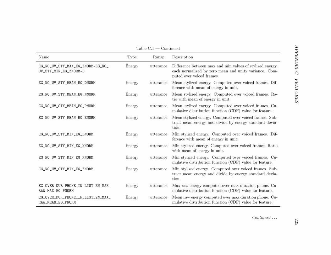
AP
PE
ND
IXC
.FE
AT
UR
ES
225
Table C.1 — Continued
Name Type Range Description
EG_NO_UV_STY_MAX_EG_ZNORM-EG_NO_
UV_STY_MIN_EG_ZNORM-D
Energy utterance Difference between max and min values of stylized energy,each normalized by zero mean and unity variance. Com-puted over voiced frames.
EG_NO_UV_STY_MEAN_EG_DNORM Energy utterance Mean stylized energy. Computed over voiced frames. Dif-ference with mean of energy in unit.
EG_NO_UV_STY_MEAN_EG_NNORM Energy utterance Mean stylized energy. Computed over voiced frames. Ra-tio with mean of energy in unit.
EG_NO_UV_STY_MEAN_EG_PNORM Energy utterance Mean stylized energy. Computed over voiced frames. Cu-mulative distribution function (CDF) value for feature.
EG_NO_UV_STY_MEAN_EG_ZNORM Energy utterance Mean stylized energy. Computed over voiced frames. Sub-tract mean energy and divide by energy standard devia-tion.
EG_NO_UV_STY_MIN_EG_DNORM Energy utterance Min stylized energy. Computed over voiced frames. Dif-ference with mean of energy in unit.
EG_NO_UV_STY_MIN_EG_NNORM Energy utterance Min stylized energy. Computed over voiced frames. Ratiowith mean of energy in unit.
EG_NO_UV_STY_MIN_EG_PNORM Energy utterance Min stylized energy. Computed over voiced frames. Cu-mulative distribution function (CDF) value for feature.
EG_NO_UV_STY_MIN_EG_ZNORM Energy utterance Min stylized energy. Computed over voiced frames. Sub-tract mean energy and divide by energy standard devia-tion.
EG_OVER_DUR_PHONE_IN_LIST_ZN_MAX_
RAW_MAX_EG_PNORM
Energy utterance Max raw energy computed over max duration phone. Cu-mulative distribution function (CDF) value for feature.
EG_OVER_DUR_PHONE_IN_LIST_ZN_MAX_
RAW_MEAN_EG_PNORM
Energy utterance Mean raw energy computed over max duration phone. Cu-mulative distribution function (CDF) value for feature.
Continued . . .

AP
PE
ND
IXC
.FE
AT
UR
ES
226
Table C.1 — Continued
Name Type Range Description
EG_OVER_DUR_PHONE_IN_LIST_ZN_MAX_
RAW_MIN_EG_PNORM
Energy utterance Min raw energy computed over max duration phone. Cu-mulative distribution function (CDF) value for feature.
EG_OVER_DUR_PHONE_IN_LIST_ZN_MAX_
STY_MAX_EG_PNORM
Energy utterance Max stylized energy computed over max duration phone.Cumulative distribution function (CDF) value for feature.
EG_OVER_DUR_PHONE_IN_LIST_ZN_MAX_
STY_MEAN_EG_PNORM
Energy utterance Mean stylized energy computed over max duration phone.Cumulative distribution function (CDF) value for feature.
EG_OVER_DUR_PHONE_IN_LIST_ZN_MAX_
STY_MIN_EG_PNORM
Energy utterance Min stylized energy computed over max duration phone.Cumulative distribution function (CDF) value for feature.
EG_RAW_FIRST_EG_PNORM Energy utterance First value of raw energy. Cumulative distribution function(CDF) value for feature.
EG_RAW_LAST_EG_PNORM Energy utterance Last value of raw energy. Cumulative distribution function(CDF) value for feature.
EG_RAW_MAX_EG_DNORM Energy utterance Maximum raw energy. Difference with mean of energy inunit.
EG_RAW_MAX_EG_NNORM Energy utterance Maximum raw energy. Ratio with mean of energy in unit.
EG_RAW_MAX_EG_PNORM Energy utterance Maximum raw energy. Cumulative distribution function(CDF) value for feature.
EG_RAW_MAX_EG_ZNORM Energy utterance Maximum raw energy. Subtract mean energy and divideby energy standard deviation.
EG_RAW_MEAN_EG_DNORM Energy utterance Mean raw energy. Difference with mean of energy in unit.
EG_RAW_MEAN_EG_NNORM Energy utterance Mean raw energy. Ratio with mean of energy in unit.
EG_RAW_MEAN_EG_PNORM Energy utterance Mean raw energy. Cumulative distribution function (CDF)value for feature.
EG_RAW_MEAN_EG_ZNORM Energy utterance Mean raw energy. Subtract mean energy and divide byenergy standard deviation.
Continued . . .

AP
PE
ND
IXC
.FE
AT
UR
ES
227
Table C.1 — Continued
Name Type Range Description
EG_RAW_MIN_EG_DNORM Energy utterance Min raw energy. Difference with mean of energy in unit.
EG_RAW_MIN_EG_NNORM Energy utterance Min raw energy. Ratio with mean of energy in unit.
EG_RAW_MIN_EG_PNORM Energy utterance Min raw energy. Cumulative distribution function (CDF)value for feature.
EG_RAW_MIN_EG_ZNORM Energy utterance Min raw energy. Subtract mean energy and divide by en-ergy standard deviation.
F0_MEDFILT_MAX-F0_MEDFILT_MAX-D F0 utterance Difference between max and min median filtered pitch.
F0_MEDFILT_MAX_ZNORM-F0_MEDFILT_
MAX_ZNORM-D
F0 utterance Difference between max and min median filtered pitch.Subtracted mean and divided by standard deviation.
F0_NUM_D_FRAMES F0 utterance Number of doubled pitch frames.
F0_NUM_D_FRAMES-F0_NUM_V_FRAMES-R F0 utterance Number of doubled pitch frames. Ratio with number ofvoiced pitch frames.
F0_NUM_D_FRAMES-UNIT_LENGTH-R F0 utterance Number of doubled pitch frames. Ratio with unit length.
F0_NUM_F_FRAMES F0 utterance Number of falling pitch frames.
F0_NUM_F_FRAMES-F0_NUM_V_FRAMES-R F0 utterance Number of falling pitch frames. Ratio with number ofvoiced pitch frames.
F0_NUM_F_FRAMES-UNIT_LENGTH-R F0 utterance Number of falling pitch frames. Ratio with unit length.
F0_NUM_H_FRAMES F0 utterance Number of halved pitch frames.
F0_NUM_H_FRAMES-F0_NUM_V_FRAMES-R F0 utterance Number of halved pitch frames. Ratio with number ofvoiced pitch frames.
F0_NUM_H_FRAMES-UNIT_LENGTH-R F0 utterance Number of halved pitch frames. Ratio with unit length.
F0_NUM_R_FRAMES F0 utterance Number of rising pitch frames.
F0_NUM_R_FRAMES-F0_NUM_V_FRAMES-R F0 utterance Number of rising pitch frames. Ratio with number ofvoiced pitch frames.
Continued . . .
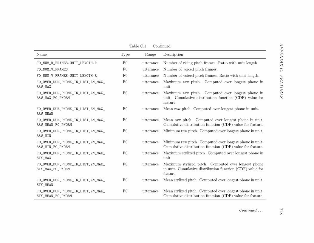
AP
PE
ND
IXC
.FE
AT
UR
ES
228
Table C.1 — Continued
Name Type Range Description
F0_NUM_R_FRAMES-UNIT_LENGTH-R F0 utterance Number of rising pitch frames. Ratio with unit length.
F0_NUM_V_FRAMES F0 utterance Number of voiced pitch frames.
F0_NUM_V_FRAMES-UNIT_LENGTH-R F0 utterance Number of voiced pitch frames. Ratio with unit length.
F0_OVER_DUR_PHONE_IN_LIST_ZN_MAX_
RAW_MAX
F0 utterance Maximum raw pitch. Computed over longest phone inunit.
F0_OVER_DUR_PHONE_IN_LIST_ZN_MAX_
RAW_MAX_F0_PNORM
F0 utterance Maximum raw pitch. Computed over longest phone inunit. Cumulative distribution function (CDF) value forfeature.
F0_OVER_DUR_PHONE_IN_LIST_ZN_MAX_
RAW_MEAN
F0 utterance Mean raw pitch. Computed over longest phone in unit.
F0_OVER_DUR_PHONE_IN_LIST_ZN_MAX_
RAW_MEAN_F0_PNORM
F0 utterance Mean raw pitch. Computed over longest phone in unit.Cumulative distribution function (CDF) value for feature.
F0_OVER_DUR_PHONE_IN_LIST_ZN_MAX_
RAW_MIN
F0 utterance Minimum raw pitch. Computed over longest phone in unit.
F0_OVER_DUR_PHONE_IN_LIST_ZN_MAX_
RAW_MIN_F0_PNORM
F0 utterance Minimum raw pitch. Computed over longest phone in unit.Cumulative distribution function (CDF) value for feature.
F0_OVER_DUR_PHONE_IN_LIST_ZN_MAX_
STY_MAX
F0 utterance Maximum stylized pitch. Computed over longest phone inunit.
F0_OVER_DUR_PHONE_IN_LIST_ZN_MAX_
STY_MAX_F0_PNORM
F0 utterance Maximum stylized pitch. Computed over longest phonein unit. Cumulative distribution function (CDF) value forfeature.
F0_OVER_DUR_PHONE_IN_LIST_ZN_MAX_
STY_MEAN
F0 utterance Mean stylized pitch. Computed over longest phone in unit.
F0_OVER_DUR_PHONE_IN_LIST_ZN_MAX_
STY_MEAN_F0_PNORM
F0 utterance Mean stylized pitch. Computed over longest phone in unit.Cumulative distribution function (CDF) value for feature.
Continued . . .

AP
PE
ND
IXC
.FE
AT
UR
ES
229
Table C.1 — Continued
Name Type Range Description
F0_OVER_DUR_PHONE_IN_LIST_ZN_MAX_
STY_MIN
F0 utterance Minimum stylized pitch. Computed over longest phone inunit.
F0_OVER_DUR_PHONE_IN_LIST_ZN_MAX_
STY_MIN_F0_PNORM
F0 utterance Minimum stylized pitch. Computed over longest phone inunit. Cumulative distribution function (CDF) value forfeature.
F0_RAW_FIRST F0 utterance First raw pitch.
F0_RAW_FIRST_F0_PNORM F0 utterance First raw pitch. Cumulative distribution function (CDF)value for feature.
F0_RAW_LAST F0 utterance Last raw pitch.
F0_RAW_LAST_F0_PNORM F0 utterance Last raw pitch. Cumulative distribution function (CDF)value for feature.
F0_RAW_MAX F0 utterance Maximum raw pitch.
F0_RAW_MAX-F0_RAW_MAX-D F0 utterance Difference between max and min raw pitch.
F0_RAW_MAX_ZNORM-F0_RAW_MAX_
ZNORM-D
F0 utterance Difference between max and min raw pitch. Subtractedmean and divided by standard deviation.
F0_RAW_MAX_F0_DNORM F0 utterance Maximum raw pitch. Difference with mean of pitch in unit.
F0_RAW_MAX_F0_NNORM F0 utterance Maximum raw pitch. Ratio with mean of pitch in unit.
F0_RAW_MAX_F0_PNORM F0 utterance Maximum raw pitch. Cumulative distribution function(CDF) value for feature.
F0_RAW_MAX_F0_ZNORM F0 utterance Maximum raw pitch. Subtract mean pitch and divide bypitch standard deviation.
F0_RAW_MEAN F0 utterance Mean raw pitch.
F0_RAW_MEAN_F0_DNORM F0 utterance Mean raw pitch. Difference with mean of pitch in unit.
F0_RAW_MEAN_F0_NNORM F0 utterance Mean raw pitch. Ratio with mean of pitch in unit.
Continued . . .

AP
PE
ND
IXC
.FE
AT
UR
ES
230
Table C.1 — Continued
Name Type Range Description
F0_RAW_MEAN_F0_PNORM F0 utterance Mean raw pitch. Cumulative distribution function (CDF)value for feature.
F0_RAW_MEAN_F0_ZNORM F0 utterance Mean raw pitch. Subtract mean pitch and divide by pitchstandard deviation.
F0_RAW_MIN F0 utterance Minimum raw pitch.
F0_RAW_MIN_F0_DNORM F0 utterance Minimum raw pitch. Difference with mean of pitch in unit.
F0_RAW_MIN_F0_NNORM F0 utterance Minimum raw pitch. Ratio with mean of pitch in unit.
F0_RAW_MIN_F0_PNORM F0 utterance Minimum raw pitch. Cumulative distribution function(CDF) value for feature.
F0_RAW_MIN_F0_ZNORM F0 utterance Minimum raw pitch. Subtract mean pitch and divide bypitch standard deviation.
F0_STY_FIRST F0 utterance First stylized pitch.
F0_STY_FIRST_F0_PNORM F0 utterance First stylized pitch. Cumulative distribution function(CDF) value for feature.
F0_STY_LAST F0 utterance Last stylized pitch.
F0_STY_LAST_F0_PNORM F0 utterance Last stylized pitch. Cumulative distribution function(CDF) value for feature.
F0_STY_MAX F0 utterance Maximum stylized pitch.
F0_STY_MAX-F0_STY_MAX-D F0 utterance Difference between max and min stylized pitch.
F0_STY_MAX_ZNORM-F0_STY_MAX_
ZNORM-D
F0 utterance Difference between max and min stylized pitch. Subtractedmean and divided by standard deviation.
F0_STY_MAX_F0_DNORM F0 utterance Maximum stylized pitch. Difference with mean of pitch inunit.
F0_STY_MAX_F0_NNORM F0 utterance Maximum stylized pitch. Ratio with mean of pitch in unit.
Continued . . .

AP
PE
ND
IXC
.FE
AT
UR
ES
231
Table C.1 — Continued
Name Type Range Description
F0_STY_MAX_F0_PNORM F0 utterance Maximum stylized pitch. Cumulative distribution function(CDF) value for feature.
F0_STY_MAX_F0_ZNORM F0 utterance Maximum stylized pitch. Subtract mean pitch and divideby pitch standard deviation.
F0_STY_MEAN F0 utterance Mean stylized pitch.
F0_STY_MEAN_F0_DNORM F0 utterance Mean stylized pitch. Difference with mean of pitch in unit.
F0_STY_MEAN_F0_NNORM F0 utterance Mean stylized pitch. Ratio with mean of pitch in unit.
F0_STY_MEAN_F0_PNORM F0 utterance Mean stylized pitch. Cumulative distribution function(CDF) value for feature.
F0_STY_MEAN_F0_ZNORM F0 utterance Mean stylized pitch. Subtract mean pitch and divide bypitch standard deviation.
F0_STY_MIN F0 utterance Minimum stylized pitch.
F0_STY_MIN_F0_DNORM F0 utterance Minimum stylized pitch. Difference with mean of pitch inunit.
F0_STY_MIN_F0_NNORM F0 utterance Minimum stylized pitch. Ratio with mean of pitch in unit.
F0_STY_MIN_F0_PNORM F0 utterance Minimum stylized pitch. Cumulative distribution function(CDF) value for feature.
F0_STY_MIN_F0_ZNORM F0 utterance Minimum stylized pitch. Subtract mean pitch and divideby pitch standard deviation.
F0_SLOPES_AVERAGE F0 utterance Average pitch slope.
F0_SLOPES_FIRST F0 utterance First pitch slope.
F0_SLOPES_LAST F0 utterance Lasst pitch slope.
F0_SLOPES_LENGTH_FIRST F0 utterance Length in frames of first pitch slope.
Continued . . .

AP
PE
ND
IXC
.FE
AT
UR
ES
232
Table C.1 — Continued
Name Type Range Description
F0_SLOPES_LENGTH_FIRST-UNIT_
LENGTH-R
F0 utterance Ratio of length in frames of first pitch slope and unitlength.
F0_SLOPES_LENGTH_LAST F0 utterance Length in frames of last pitch slope.
F0_SLOPES_LENGTH_LAST-UNIT_
LENGTH-R
F0 utterance Ratio of length in frames of last pitch slope and unit length.
F0_SLOPES_MAX_NEG F0 utterance Maximum negative pitch slope.
F0_SLOPES_MAX_POS F0 utterance Maximum positive pitch slope.
F0_SLOPES_NOHD_AVERAGE F0 utterance Average pitch slope. Computed in frames with no doublingor halving.
F0_SLOPES_NOHD_LENGTH_FIRST F0 utterance Length in frames of first pitch slope. Computed in frameswith no doubling or halving.
F0_SLOPES_NOHD_LENGTH_FIRST-UNIT_
LENGTH-R
F0 utterance Ratio of length in frames of first pitch slope and unitlength. Computed in frames with no doubling or halving.
F0_SLOPES_NOHD_LENGTH_FIRST-UNIT_
LENGTH-R
F0 utterance Ratio of length in frames of first pitch slope and unitlength. Computed in frames with no doubling or halving.
F0_SLOPES_NOHD_LENGTH_LAST F0 utterance Length in frames of last pitch slope. Computed in frameswith no doubling or halving.
F0_SLOPES_NOHD_LENGTH_LAST-UNIT_
LENGTH-R
F0 utterance Ratio of length in frames of last pitch slope and unit length.Computed in frames with no doubling or halving.
F0_SLOPES_NOHD_MAX_NEG F0 utterance Maximum negative pitch slope. Computed in frames withno doubling or halving.
F0_SLOPES_NOHD_MAX_POS F0 utterance Maximum positive pitch slope. Computed in frames withno doubling or halving.
F0_SLOPES_NOHD_NUM_CHANGES F0 utterance Number of slope changes in unit. Computed in frames withno doubling or halving.
Continued . . .

AP
PE
ND
IXC
.FE
AT
UR
ES
233
Table C.1 — Continued
Name Type Range Description
F0_SLOPES_NOHD_NUM_CHANGES-F0_NUM_
V_FRAMES-R
F0 utterance Ratio of number of slope changes in unit by number ofvoiced frames. Computed in frames with no doubling orhalving.
F0_SLOPES_NOHD_NUM_CHANGES-UNIT_
LENGTH-R
F0 utterance Ratio of number of slope changes in unit by the unit length.Computed in frames with no doubling or halving.