Embed Size (px)
Citation preview

Scholars' Mine Scholars' Mine
Doctoral Dissertations Student Theses and Dissertations
Summer 2013
Detecting and locating electronic devices using their unintended Detecting and locating electronic devices using their unintended
electromagnetic emissions electromagnetic emissions
Colin Stagner
Follow this and additional works at: https://scholarsmine.mst.edu/doctoral_dissertations
Part of the Electrical and Computer Engineering Commons
Department: Electrical and Computer Engineering Department: Electrical and Computer Engineering
Recommended Citation Recommended Citation Stagner, Colin, "Detecting and locating electronic devices using their unintended electromagnetic emissions" (2013). Doctoral Dissertations. 2152. https://scholarsmine.mst.edu/doctoral_dissertations/2152
This thesis is brought to you by Scholars' Mine, a service of the Missouri S&T Library and Learning Resources. This work is protected by U. S. Copyright Law. Unauthorized use including reproduction for redistribution requires the permission of the copyright holder. For more information, please contact [email protected].

DETECTING AND LOCATING ELECTRONIC DEVICES USING THEIR
UNINTENDED ELECTROMAGNETIC EMISSIONS
by
COLIN BLAKE STAGNER
A DISSERTATION
Presented to the Faculty of the Graduate School of the
MISSOURI UNIVERSITY OF SCIENCE AND TECHNOLOGY
In Partial Fulfillment of the Requirements for the Degree
DOCTOR OF PHILOSOPHY
in
ELECTRICAL & COMPUTER ENGINEERING
2013
Approved by
Dr. Steve Grant, Advisor
Dr. Daryl Beetner
Dr. Kurt Kosbar
Dr. Reza Zoughi
Dr. Bruce McMillin

Copyright 2013
Colin Blake Stagner
All Rights Reserved

iii
ABSTRACT
Electronically-initiated explosives can have unintended electromagnetic emis-
sions which propagate through walls and sealed containers. These emissions, if prop-
erly characterized, enable the prompt and accurate detection of explosive threats.
The following dissertation develops and evaluates techniques for detecting and locat-
ing common electronic initiators. The unintended emissions of radio receivers and
microcontrollers are analyzed. These emissions are low-power radio signals that result
from the device’s normal operation.
In the first section, it is demonstrated that arbitrary signals can be injected
into a radio receiver’s unintended emissions using a relatively weak stimulation signal.
This effect is called stimulated emissions. The performance of stimulated emissions
is compared to passive detection techniques. The novel technique offers a 5 to 10 dB
sensitivity improvement over passive methods for detecting radio receivers.
The second section develops a radar-like technique for accurately locating
radio receivers. The radar utilizes the stimulated emissions technique with wideband
signals. A radar-like system is designed and implemented in hardware. Its accuracy
tested in a noisy, multipath-rich, indoor environment. The proposed radar can locate
superheterodyne radio receivers with a root mean square position error less than
5 meters when the SNR is 15 dB or above.
In the third section, an analytic model is developed for the unintended emis-
sions of microcontrollers. It is demonstrated that these emissions consist of a periodic
train of impulses. Measurements of an 8051 microcontroller validate this model. The
model is used to evaluate the noise performance of several existing algorithms. Results
indicate that the pitch estimation techniques have a 4 dB sensitivity improvement
over epoch folding algorithms.

iv
ACKNOWLEDGMENTS
The author would like to thank his advisor, Dr. Steve Grant, for his insightful
guidance throughout each stage of these projects. Dr. Grant, who introduced me to
the realm of signal processing, assisted greatly with many of the measurements found
in this text. His endless patience, and willingness to share his decades of research
experience, are most appreciated. I would also like to thank Dr. Daryl Beetner’s
minute attention to detail and continuous revisions, which have greatly improved the
quality of my writing and sped my papers along to publication.
My friends and fellow PhDs, Dr. Chris Osterwise and Dr. Dan Krus, have been
with me every step of the way, and their keen observations have kept my dissertation
on track. Cisa, who is wise beyond her years, has offered me counsel and guidance
which has improved every aspect of my life. Our dog Lea should also be recognized
for her brief—though futile—attempt at grading.
Considerable financial support for this research was provided by the U.S. De-
partment of Homeland Security under Award Number 2008-ST-061-ED0001, the Na-
tional Science Foundation under Grant No. 0855878, and the Wilkens Missouri En-
dowment. The author would also like to thank the years of steady financial support
provided by Missouri S&T’s Chancellor’s Fellowship program, which has enabled me
to complete my required coursework.
Credit is also due to the volunteer developers of GNU Radio, GNU Octave,
and the various other open source projects which are an integral part of this research.
Their time and efforts have enabled this contribution to science.
Finally, I would like to thank DeeDee for her unwavering dedication and
boundless capacity for self-expression: you make each day an adventure unto itself.

v
TABLE OF CONTENTS
Page
ABSTRACT . . . . . . . . . . . . . . . . . . . . . . . . . . . . . . . . . . . . . . . . . . . . . . . . . . . . . . . . . . . . . . . . . . . iii
ACKNOWLEDGMENTS . . . . . . . . . . . . . . . . . . . . . . . . . . . . . . . . . . . . . . . . . . . . . . . . . . . . . . iv
LIST OF ILLUSTRATIONS . . . . . . . . . . . . . . . . . . . . . . . . . . . . . . . . . . . . . . . . . . . . . . . . . . . viii
LIST OF TABLES. . . . . . . . . . . . . . . . . . . . . . . . . . . . . . . . . . . . . . . . . . . . . . . . . . . . . . . . . . . . . x
SECTION
1 INTRODUCTION. . . . . . . . . . . . . . . . . . . . . . . . . . . . . . . . . . . . . . . . . . . . . . . . . . . . . . . . . . 1
2 DETECTING SUPERHETERODYNE RECEIVERS . . . . . . . . . . . . . . . . . . . . . . . 5
2.1 MEASURING THE UNINTENDED EMISSIONS . . . . . . . . . . . 7
2.1.1 Near-Field Analysis . . . . . . . . . . . . . . . . . . . . . . . . 8
2.1.2 Time Domain Analysis . . . . . . . . . . . . . . . . . . . . . . 11
2.1.3 Frequency Selection . . . . . . . . . . . . . . . . . . . . . . . . 17
2.2 DESIGNING THE RADIO DETECTORS . . . . . . . . . . . . . . . 18
2.2.1 Periodogram Detector . . . . . . . . . . . . . . . . . . . . . . 18
2.2.2 Matched Filter Detector: The Novel Approach . . . . . . . . . 20
2.3 THEORETICAL PERFORMANCE . . . . . . . . . . . . . . . . . . 22
2.3.1 Emulating GMRS Emissions . . . . . . . . . . . . . . . . . . . 23
2.3.2 Quantitative Results . . . . . . . . . . . . . . . . . . . . . . . 23
2.3.3 Qualitative Results . . . . . . . . . . . . . . . . . . . . . . . . 24
2.4 CONCLUSION . . . . . . . . . . . . . . . . . . . . . . . . . . . . . . 26

vi
3 LOCATING SUPERHETERODYNE RECEIVERS . . . . . . . . . . . . . . . . . . . . . . . . . 27
3.1 METHODS . . . . . . . . . . . . . . . . . . . . . . . . . . . . . . . . 29
3.1.1 Wideband Stimulated Emissions . . . . . . . . . . . . . . . . . 29
3.1.2 Bandwidth Measurements . . . . . . . . . . . . . . . . . . . . 32
3.1.3 Time of Arrival Method . . . . . . . . . . . . . . . . . . . . . 34
3.1.4 Hardware Realization . . . . . . . . . . . . . . . . . . . . . . . 36
3.2 RESULTS . . . . . . . . . . . . . . . . . . . . . . . . . . . . . . . . . 39
3.2.1 Indoor Test . . . . . . . . . . . . . . . . . . . . . . . . . . . . 40
3.2.2 Outdoor Test . . . . . . . . . . . . . . . . . . . . . . . . . . . 40
3.3 DISCUSSION . . . . . . . . . . . . . . . . . . . . . . . . . . . . . . . 42
3.3.1 Analysis of Accuracy . . . . . . . . . . . . . . . . . . . . . . . 43
3.3.2 Sources of Error . . . . . . . . . . . . . . . . . . . . . . . . . . 43
3.3.3 Device Limitations . . . . . . . . . . . . . . . . . . . . . . . . 45
3.4 CONCLUSION . . . . . . . . . . . . . . . . . . . . . . . . . . . . . . 45
4 DETECTING AND IDENTIFYING MICROCONTROLLERS. . . . . . . . . . . . . . 47
4.1 METHODS . . . . . . . . . . . . . . . . . . . . . . . . . . . . . . . . 49
4.1.1 Autoregressive Model and Detector . . . . . . . . . . . . . . . 49
4.1.2 Pitch Estimation . . . . . . . . . . . . . . . . . . . . . . . . . 54
4.1.3 Fast Folding Algorithm . . . . . . . . . . . . . . . . . . . . . . 57
4.2 RESULTS . . . . . . . . . . . . . . . . . . . . . . . . . . . . . . . . . 59
4.2.1 Model Validation . . . . . . . . . . . . . . . . . . . . . . . . . 59
4.2.2 Simulated Environment . . . . . . . . . . . . . . . . . . . . . 65
4.2.3 Simulation Results . . . . . . . . . . . . . . . . . . . . . . . . 67
4.3 DISCUSSION . . . . . . . . . . . . . . . . . . . . . . . . . . . . . . . 70
4.3.1 Constant False Alarm Rate . . . . . . . . . . . . . . . . . . . 71
4.3.2 Jitter . . . . . . . . . . . . . . . . . . . . . . . . . . . . . . . . 72

vii
4.4 CONCLUSION . . . . . . . . . . . . . . . . . . . . . . . . . . . . . . 75
APPENDIX . . . . . . . . . . . . . . . . . . . . . . . . . . . . . . . . . . . . . . . . . . . . . . . . . . . . . . . . . . . . . . . . . . . 77
BIBLIOGRAPHY . . . . . . . . . . . . . . . . . . . . . . . . . . . . . . . . . . . . . . . . . . . . . . . . . . . . . . . . . . . . . 86
VITA . . . . . . . . . . . . . . . . . . . . . . . . . . . . . . . . . . . . . . . . . . . . . . . . . . . . . . . . . . . . . . . . . . . . . . . . . . 93

viii
LIST OF ILLUSTRATIONS
Figure Page
1.1 Each component of an explosive device has a specific environmentalsignature. . . . . . . . . . . . . . . . . . . . . . . . . . . . . . . . . . 2
2.1 A superheterodyne receiver front-end. . . . . . . . . . . . . . . . . . . 8
2.2 A comparison of unstimulated and stimulated emissions. . . . . . . . 10
2.3 Spectrogram of up-mixing emissions. . . . . . . . . . . . . . . . . . . 14
2.4 Spectrogram of up-mixing emissions from a second GMRS receivermodel. . . . . . . . . . . . . . . . . . . . . . . . . . . . . . . . . . . . 15
2.5 Magnitude of local oscillator emissions when the radio was not stimu-lated. . . . . . . . . . . . . . . . . . . . . . . . . . . . . . . . . . . . . 15
2.6 A passive detection algorithm using periodograms. . . . . . . . . . . . 19
2.7 A stimulated emissions detection algorithm using matched filters. . . 22
2.8 Receiver Operating Characteristics of both the matched filter detectorand the periodogram detector. . . . . . . . . . . . . . . . . . . . . . . 25
3.1 The stimulated emissions detection process. . . . . . . . . . . . . . . 28
3.2 A superheterodyne front-end which uses low-side injection. . . . . . . 30
3.3 Stimulated emissions of a GMRS receiver. . . . . . . . . . . . . . . . 33
3.4 Hardware realization of the stimulated emissions radar. . . . . . . . . 37
3.5 Indoor range estimates of the GMRS receiver and the wideband scanner. 42
3.6 Root mean square error performance of the stimulated emissions radar. 44
4.1 The current draw of a CMOS device. . . . . . . . . . . . . . . . . . . 50
4.2 An autoregressive process. . . . . . . . . . . . . . . . . . . . . . . . . 52
4.3 Welch periodogram of the CMOS clock pulses shown in Figure 4.1. . 55
4.4 In epoch folding, a periodic signal is estimated by folding (i.e., sum-ming) the received data from successive periods. . . . . . . . . . . . . 58
4.5 The embedded system under test. . . . . . . . . . . . . . . . . . . . . 60

ix
4.6 Time and frequency-domain views of an 8051 microcontroller’s emissions. 61
4.7 Epoch folding of 8051 electromagnetic emissions. . . . . . . . . . . . . 63
4.8 The epoch-folded 8051 emissions and the ideal CMOS pulse determinedby linear prediction. . . . . . . . . . . . . . . . . . . . . . . . . . . . 64
4.9 The minimum description length (MDL) statistic. . . . . . . . . . . . 65
4.10 Simulation results for CMOS signal in white noise. . . . . . . . . . . . 68
4.11 Simulation results for the weak sinusoid and strong sinusoid. . . . . . 69
4.12 The CFAR algorithm estimates the noise level for each bin using thesurrounding bins. . . . . . . . . . . . . . . . . . . . . . . . . . . . . . 73
4.13 Simulation results for a jittery CMOS signal. . . . . . . . . . . . . . . 74
x
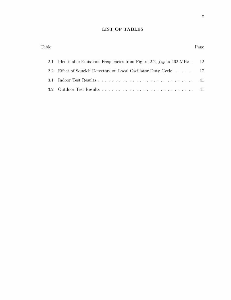
LIST OF TABLES
Table Page
2.1 Identifiable Emissions Frequencies from Figure 2.2, fRF ≈ 462 MHz . 12
2.2 Effect of Squelch Detectors on Local Oscillator Duty Cycle . . . . . . 17
3.1 Indoor Test Results . . . . . . . . . . . . . . . . . . . . . . . . . . . . 41
3.2 Outdoor Test Results . . . . . . . . . . . . . . . . . . . . . . . . . . . 41

1. INTRODUCTION
Remote detection of improvised explosive devices is essential to guaranteeing
safety in conflict-prone environments. At present, there are three main techniques
for detecting explosive devices: manual search, portal screening, and chemical trace
detection. Manual search techniques utilize explosives ordinance disposal (EOD)
technicians to find and neutralize explosives. Clearing an area is a time-consuming,
dangerous task which can expose personnel and resources, such as robots, to risk.
In portal screening techniques, a secure area is defined, and persons entering the
area are subject to a thorough search. This technique results in large delays and
great expense: the United States spends $4.8 billion U.S. dollars per year on security
checkpoints for its airports [2].
Both of these search methods are often augmented with some type of explo-
sives-detection sensor. Chemical traces are the most specific indication that explo-
sives are present, and others have developed a number of different techniques for
detecting them. By characterizing the chemical composition and behavior of high-
explosives, such as ammonium nitrate [3], it is possible to build more reliable sen-
sors. Terahertz imaging techniques offer improved portal screening with an inherent
explosives-detection capability [4].
Sensors that are capable of detecting explosives from outside of their effective
range are an important, emerging area of research. This search strategy is commonly
referred to as standoff detection. These sensors must cope with the low signal-to-
noise ratio (SNR) which is inherent to long-range detection. Raman spectroscopy is
one such technique. It has the potential to detect chemical traces on surfaces, using
lasers, at great distances [5].

2
These techniques have inherent disadvantages, however. Scanning a large
area can be extremely time consuming. Obstacles like hills, trees, and buildings
can prevent detection. All chemical trace systems, including canines, have difficulty
detecting explosives which are housed in air-tight containers [6]. Indirect methods,
which detect the non-explosive components, can be useful in these situations.
Explosive devices typically contain at least three components: propellant, a
payload, and an initiator. Each of these components, which are shown conceptually
in Figure 1.1, provides a different opportunity for detection. Chemical traces are the
most specific indication that explosives are present, but the payload and initiator can
have specific, detectable environmental signatures as well.
One way to indirectly detect potential explosive devices is to detect the ini-
tiator. Explosive devices are commonly initiated using proximity sensors or remote
triggers [7, 8]. These initiators are electronic devices which generate and process
high-frequency signals. Such signals can radiate from resonant features in the de-
vice’s printed circuit board (PCB) and packaging, escaping into the environment as
unintended electromagnetic emissions.
Unlike chemical traces, electromagnetic emissions can propagate freely through
closed containers and vehicles. Others have demonstrated that these emissions can
Initiator Payload
Electromagnetic
Emissions
Chemical
Traces
Propellant
Magnetic
Resonance
Figure 1.1: Each component of an explosive device has a specific environmental sig-nature.

3
reveal information about a device’s purpose and internal state [9], making it possible
to determine what types of devices are present. By detecting potential initiators, it
is possible to infer the presence of an explosive threat. This approach makes non-
line-of-sight device detection feasible at relatively long range.
In order to provide a substantial advantage over the direct methods, an elec-
tronic initiator detector must offer high sensitivity and selectivity. A high-sensitivity
detector should be capable of detecting weak, unintended electromagnetic emissions—
the power of which is strictly limited by regulation [10]. While an extraordinary
variety of electronic devices exist, a detector should be capable of separating devices
which pose an explosive-related threat from devices which do not. Selectivity and
sensitivity can be improved by using specific knowledge of the emissions’ character-
istics.
The purpose of this work is to improve techniques for detecting specific types of
electronic initiators. Radio receivers of every variety, such as doorbells, automobile
keyfobs, two-way radios, and cellular telephones, can be used as remote initiators
[8,11]. Devices may also incorporate microcontrollers and other clocked, digital logic
systems for either timing or control purposes. This dissertation includes three papers
on the detection, location, and identification of these electronic devices.
The first paper, which was originally published as [12], presents a new tech-
nique for detecting superheterodyne radio receivers. This technique, which is known
as stimulated emissions, was originally developed for super-regenerative receivers.
The extension allows stimulated emissions to work with a wide variety of new de-
vices. Numerical simulations indicate that the theoretical performance of stimulated
emissions far exceeds that of existing, passive techniques.
In the second paper, new measurements suggest that superheterodyne re-
ceivers are sensitive to a much wider band of frequencies than they are designed to

4
receive. As published in [13], this new information enables the development of a time-
of-arrival technique for locating radio receivers. Radar theory is combined with the
stimulated emissions technique to determine the range to radio receivers. A hardware
test platform is developed, and the accuracy of this technique is tested in both indoor
and outdoor environments.
For the third paper, techniques are tested for positively identifying microcon-
trollers using their unintended electromagnetic emissions. It is demonstrated that
microcontrollers have clock-dependent emissions that are impulsive and periodic. An
autoregressive model is developed for simulating, and for detecting, clock emissions.
Several algorithms, including one novel algorithm, are proposed for detecting these
emissions. The applicability and usefulness of each algorithm as a clock-circuit de-
tector is considered and tested in a simulated environment.

5
2. DETECTING SUPERHETERODYNE RECEIVERS
Advances in electronics and RF design have made radio receivers smaller,
cheaper, and more common than ever before. These new devices enable a plethora of
innovative applications, but they can also be used maliciously to initiate explosives.
One way to indirectly locate potential explosive devices is to locate the radio receiver,
thus mitigating this threat. Radio receivers use many different high frequency signals
that readily escape into the environment, resulting in unintended electromagnetic
emissions. It is possible to detect radio receivers using these unintended electromag-
netic emissions [14–17].
While modern devices use a variety of radio receiver designs, the superhetero-
dyne receiver remains one of the most common. Superheterodyne receivers trans-
late high-frequency signals to a lower frequency, making them ideal for reproducing
high-quality voice and data signals. Broadcast radio receivers, cellular phones, and
two-way radios frequently incorporate superheterodyne receivers.
It is well-known that superheterodyne receivers have strong, sinusoidal local
oscillator (LO) emissions. Others have demonstrated that these emissions can be
detected using periodograms [15]. In this approach, a signal which potentially con-
tains unintended emissions is sampled, and its periodogram is computed. Each bin
is compared with a threshold, and the detector is satisfied if this threshold is ex-
ceeded. Existing research focuses on broadcast radio receivers, such as the television
sets studied in [15].
Unlike television sets, two-way radios and other battery-powered devices are
intended for intermittent use. As shown herein, two-way radios cycle their local oscil-
lators on and off to conserve power. This cycling makes the emissions non-stationary,
greatly decreasing the effectiveness of periodogram techniques. The periodogram

6
technique is also likely to be susceptible to interfering signals, since only the level of
emissions, in a narrow band, is observed. Improved detection methods are needed.
Unintended emissions can reveal information about an electronic device’s in-
ternal state [9], and radio receivers are no exception. Unlike other types of devices,
however, radio receivers are highly responsive to weak stimulation signals. Trans-
mitting a known stimulation signal to a receiver can change its unintended emissions
in a predictable manner. It is possible to detect radio receivers by comparing their
unintended emissions with the stimulation signal. This technique is called stim-
ulated emissions detection. This approach is similar to harmonic detection tech-
niques, which illuminate the electronic device with a strong stimulation and look for
“reflected” harmonics caused by interaction with non-linear electronic components.
Since the proposed technique modifies the intended signals within the device, it can
use a much lower power stimulation, can work at a longer range, and will have fewer
false-alarms than harmonic detection.
Others have developed stimulated emissions detectors for super-regenerative
receivers [14]. These systems offer improved sensitivity over unstimulated, passive
detectors, but they are incapable of detecting superheterodyne receivers. Existing
detectors affect the quenching signal in a super-regenerative circuit [17], which is not
present in superheterodyne receivers. Since stimulated emissions detectors outper-
form passive detectors for super-regenerative receivers, it is worthwhile to develop
stimulated emissions techniques for superheterodyne receivers.
The following paper describes the development of a superheterodyne radio de-
tector. Real radio receivers were measured during operation, and it is demonstrated
that certain unintended emissions have an identical complex envelope to the stimu-
lation signal. A stimulated emissions detector, which is detailed in Section 2.2.2, was
developed using matched filters. The performance of the stimulated emissions detec-
tor was compared with existing methods [15] using artificially-generated emissions.
7
The stimulated emissions approach offers substantial quantitative and qualitative ad-
vantages over existing methods, increasing the energy of the emissions and eliminating
false-positives caused by non-radio devices.
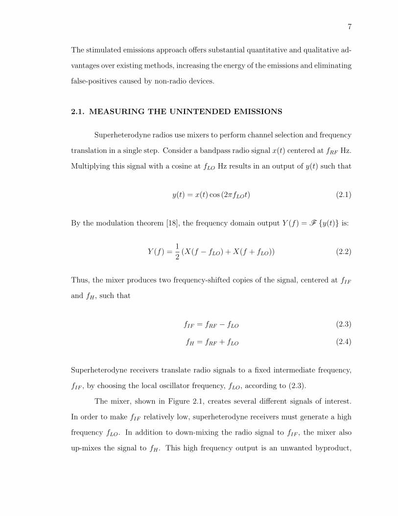
2.1. MEASURING THE UNINTENDED EMISSIONS
Superheterodyne radios use mixers to perform channel selection and frequency
translation in a single step. Consider a bandpass radio signal x(t) centered at fRF Hz.
Multiplying this signal with a cosine at fLO Hz results in an output of y(t) such that
y(t) = x(t) cos (2πfLOt) (2.1)
By the modulation theorem [18], the frequency domain output Y (f) = F {y(t)} is:
Y (f) =1
2(X(f − fLO) +X(f + fLO)) (2.2)
Thus, the mixer produces two frequency-shifted copies of the signal, centered at fIF
and fH , such that
fIF = fRF − fLO (2.3)
fH = fRF + fLO (2.4)
Superheterodyne receivers translate radio signals to a fixed intermediate frequency,
fIF , by choosing the local oscillator frequency, fLO, according to (2.3).
The mixer, shown in Figure 2.1, creates several different signals of interest.
In order to make fIF relatively low, superheterodyne receivers must generate a high
frequency fLO. In addition to down-mixing the radio signal to fIF , the mixer also
up-mixes the signal to fH . This high frequency output is an unwanted byproduct,

8
but it is easily removed with a low-order filter. Superheterodyne receivers frequently
use two or more mixer stages, and the operating frequencies of the second stage are
known herein as fIF2 and fLO2 .
Any of these frequencies, including fLO, fIF , fLO2 , fH2 , and fH , can escape
from the radio receiver as unintended emissions, as will be demonstrated in the fol-
lowing paragraphs.
2.1.1. Near-Field Analysis. Studies of the emissions from superhetero-
dyne receivers were performed using General Mobile Radio Service (GMRS) tran-
sceivers. GMRS radios are popular, “walkie-talkie” style radios with a range of
roughly five miles [19]. Their low cost, long battery life, built-in squelch codes, and
long range make them ideal for a number of uses, but they are also small and easily
concealed about a person or device. GMRS radios often incorporate superheterodyne
IF Filter
ImageRejection
Filter RF Mixer
Local Oscillator
Pow
er
RF0Frequency
IF LO Upmix
To secondstage
Figure 2.1: A superheterodyne receiver front-end. In a superheterodyne receiver,the mixer shifts the RF input both down in frequency (IF component)and up in frequency (up-mixing component). These signals are plottedconceptually above. The receiver itself keeps only the IF component;the other signals are filtered out. The up-mixing component has a highfrequency, and—before it can be filtered out—tends to radiate into theenvironment.

9
receivers that have strong stimulated emissions, making them an ideal candidate for
stimulated emissions research.
Several GMRS radios were tested in the near-field to characterize their unin-
tended emissions frequencies. The radios were placed in a transverse electromagnetic
(TEM) cell, and their unintended emissions were measured with a spectrum analyzer.
To determine the difference between unstimulated and stimulated emissions, each ra-
dio was tuned to an unoccupied channel and tested with both no stimulation and
with a continuous wave (CW) stimulation. Frequency domain emissions from one
such test are shown in Figure 2.2. By comparing measurements with and without
a stimulation, it is possible to determine if a signal is a local oscillator or a mixer
output.
Local oscillator signals are always present, regardless of whether or not the
radio is receiving a signal. Superheterodyne receivers generate LO signals using
purely internal clock sources, such as crystal oscillators [20]. Since these oscillators
are designed to maintain a constant frequency—even in the presence of strong radio
signals—it is unlikely that a typical radio signal will affect LO emissions. Since it is
difficult to determine if a radio signal is present without down-mixing, superhetero-
dyne receivers must keep their LOs active—even when no radio signal is present. Any
local oscillator emissions will therefore be frequency-invariant and will not require a
stimulation signal.
Unlike local oscillator signals, mixer outputs depend significantly on stimula-
tion input signals. From (2.2), it is clear that the mixer outputs an attenuated copy
of the input signal. If the radio is unstimulated, x(t) → 0 and the mixer’s output
y(t)→ 0, regardless of the local oscillator signal’s behavior. If the radio is stimulated,
then the mixer outputs should contain a frequency-shifted copy of the stimulation
signal—an effect that is tested in the following section. Mixer output emissions are

10
-90
-85
-80
-75
-70
-65
-60
0 100 200 300 400 500 600 700 800 900
Pow
er(d
Bm
)
Frequency (MHz)
GMRS Receiver in TEM Cell, CW Stimulation
-90
-85
-80
-75
-70
-65
-60
0 100 200 300 400 500 600 700 800 900
Pow
er(d
Bm
)
Frequency (MHz)
GMRS Receiver in TEM Cell, Unstimulated
1st IF
2nd LO
1st LO
2nd LO
1st LO
Stimulation
1st LO Up
2x 1st LO
2x 1st LO
2nd LO Up
Figure 2.2: A comparison of unstimulated and stimulated emissions. Observe thatthe 440 MHz local oscillator, labeled “1st LO,” is present in both captures,and that the 21.4 MHz (“1st IF”) and 903 MHz (“1st LO Up”) mixeroutputs are only present in the stimulated case.

11
easy to identify since they require a stimulation signal and will always vary with
respect to the stimulation.
GMRS radio receivers have identifiable local oscillator, intermediate frequency,
and up-mixing emissions. Consider the different unintended emissions in Figure 2.2,
which are enumerated in Table 2.1. fLO is a signal that is both always present and very
close to fRF , making it most likely a local oscillator signal. fIF and fH are only present
when the radio is stimulated, making them possible mixer outputs. Comparing the
estimated frequency of each emissions signal, it is clear that fIF ≈ fRF − fLO and
fH ≈ fRF + fLO. Since the measured emissions satisfy (2.3) and (2.4), they follow
the design rules for a superheterodyne receiver. Thus, fLO and fIF are the receiver’s
operating frequencies.
In the process of generating the above mathematically-required signals, GMRS
receivers may also generate other, secondary signals that become unintended emis-
sions. In Table 2.1, 2fLO and fH2 are examples of secondary emissions. High fre-
quency oscillators often have second harmonics, and the 2fLO emissions are just such
a signal. The fH2 emissions are the result of the second-stage LO mixing with the
stimulation signal. Since there is no reason for the receiver to mix these signals, this
signal is probably the result of poor electromagnetic isolation. While the secondary
emissions may be useful, they are not mathematically guaranteed to exist, and it is
possible to construct a superheterodyne receiver that does not generate them.
2.1.2. Time Domain Analysis. After determining the radios’ operating
frequencies, the unintended emissions were analyzed in the time domain. The emis-
sions were sampled with an Ettus Research Universal Software Radio Peripheral
(USRP), a software-defined radio which can both transmit and receive arbitrary radio
signals. Unlike traditional oscilloscopes, which are limited by their memory depth,
the USRP can record captures of nearly unlimited length. A more comprehensive
overview of software-defined radio is given in Appendix 5. The USRP’s frequency

12
span is quite small [21], and thus it is necessary to know the emissions’ carrier fre-
quency in advance.
GMRS receivers essentially only have two unique emissions signals. Consider
the identified emissions frequencies in Table 2.1. All emissions that do not react to
a stimulation are local oscillator signals, and all signals that react to a stimulation
are mixer products. Since all signals of the same type contain the same information,
it suffices to record one of each. As a matter of convenience, fLO was selected for
unstimulated emissions and fH for stimulated emissions.
In order to determine if the fH emissions originate from the radio’s mixer, as
postulated, several GMRS radios were tested with a stimulation signal. A repeating
5 kHz, 1024 ms linear frequency modulated (FM) chirp was up-mixed and trans-
mitted to a nearby GMRS receiver. The transmitted signal’s power was less than
200 mW, which is less than the radiated power of most GMRS radio transmitters.
The frequency modulation used a maximum carrier deviation of ∆f = 5 kHz, which
is the same standard mandated for GMRS transmitters [22]. A USRP, placed in close
proximity to the radio receiver, recorded the fH emissions. In order to ensure that
Table 2.1: Identifiable Emissions Frequencies from Figure 2.2, fRF ≈ 462 MHz
NameFrequencyEstimate(MHz)
Changeswhen
Stimulated
Description
fLO2 20.94 No 2nd Local Oscillator
fIF 21.4 Yes 1st Intermediate Frequency
fLO 441.0 No 1st Local Oscillator
fH2 483.5 Yes 2nd LO Up-mixing
2fLO 882.0 No Local Osc. Harmonic
fH 903.0 Yes 1st LO Up-mixing

13
the USRP was not simply detecting a harmonic of the stimulation signal, a control
capture was taken with no GMRS radio present.
As predicted, GMRS receivers have stimulated emissions at fH , and these
emissions are an up-mixed version of the original radio signal. The spectrogram of
the emissions near fH , shown in Figure 2.3, clearly indicates the presence of the
original stimulation signal. The complex envelope increases from 0 Hz to 5 kHz over
a period of 1024 ms, which matches the original stimulation signal.
A second measurement was taken using a different GMRS radio and a 1 kHz,
pure-tone FM sinusoid. The emissions, shown in Figure 2.4, contain peaks that are
characteristic of an FM sinusoid. At close range, It is possible to demodulate the
emissions and recover the original tone. Other tests, not detailed here, indicate that
it is possible to achieve a similar effect with arbitrary FM signals. The gaps in the
emissions in Figure 2.3 and Figure 2.4 are caused by the local oscillator cycling on
and off as it searches for a signal—a further validation that these emissions are caused
by up-mixing in the radio.
GMRS radios periodically deactivate their local oscillators when no signal is
detected. In order to quantify how the stimulation signal affects the emissions, the
radio was placed in an RF-shielded environment, and the local oscillator emissions
were recorded. Figure 2.5 shows the AM demodulation of one such recording. The
reason for this response is explained below.
Since GMRS radios are intended for intermittent use and operate on shared
spectrum, they incorporate squelch detectors to reject unwanted signals. Squelch de-
tectors prevent unwanted audio output by muting the radio’s speakers unless certain
conditions are met. The first detector, carrier squelch, uses an energy detector to
determine if a narrowband radio signal is present on the channel’s carrier frequency.
Because this channel may be shared among many users, receivers may also use tone

14
-4
-2
0
2
4
0 0.5 1 1.5 2 2.5 3 3.5 4
Fre
qu
ency
(kH
z)
Time (s)
Superheterodyne Stimulated Emissions
Fre
qu
ency
(kH
z)
Time (s)
-4
-2
0
2
4
0 0.5 1 1.5 2 2.5 3 3.5 4
Figure 2.3: Spectrogram of up-mixing emissions. These fH emissions are from aGMRS receiver, measured using the USRP. A GMRS receiver was stimu-lated with a repeating 5 kHz, 1024 ms linear FM chirp (top). The originalstimulation signal is clearly visible in the emissions (bottom). The gapsin the signal are caused by the local oscillator’s duty cycle.

15
Fre
qu
ency
(Hz)
Time (s)
GMRS Stimulated Emissions: 1 kHz FM Sinusoid
-4000
-3000
-2000
-1000
0
1000
2000
3000
4000
0 0.1 0.2 0.3 0.4 0.5 0.6 0.7 0.8 0.9
Figure 2.4: Spectrogram of up-mixing emissions from a second GMRS receiver model.The radio was stimulated with a 1 kHz frequency-modulated sinusoid,and the stimulation signal is visible in the emissions. It is possible todemodulate the emissions and recover the original tone.
-10
0
10
20
30
40
50
60
70
0 100 200 300 400 500 600
Pow
er(d
B)
Time (ms)
GMRS LO Emissions, Unstimulated
Figure 2.5: Magnitude of local oscillator emissions when the radio was not stimulated.Measured with the USRP.

16
(or code) squelch to suppress unwanted calls. Both detectors must be satisfied before
the receiver un-mutes the speaker and plays back the incoming transmission.
Under this arrangement, the squelch detectors can be in one of three possible
states. Since the squelch detectors operate in series, it is possible to have no detectors
satisfied (S0), just the carrier detector satisfied (S1), or both the carrier and the tone
detectors satisfied (S2). The tone detector is optional and can be disabled by the
radio’s operator, and in this case it is always satisfied. Each state may have different
unintended emissions, making it important to test each of them.
To investigate how the radio’s squelch detectors affect its unintended emis-
sions, the receiver was stimulated with a continuous wave (CW) signal, and the fLO
emissions were measured as before. S1 was tested by enabling the tone detector.
Since the CW stimulation was a narrowband signal that lacked any frequency mod-
ulation, it satisfied the carrier detector but not the tone detector. The tone detector
was disabled to test S2, and since the stimulation satisfied both detectors, the radio
handled it like an incoming call.
According to the above test, GMRS radios deactivate their local oscillators
whenever possible. If a receiver does not detect an incoming call (states S0 and
S1), it occasionally activates its LO to poll the channel for a signal of interest. If
the squelch detectors are not satisfied, the radio deactivates its LO. If the squelch
detectors are satisfied, the radio enters state S2, and the local oscillators are kept
continuously active in order to down-mix the entire signal.
The results of this test procedure, for one GMRS receiver, are enumerated in
Table 2.2, which shows the length of time that the local oscillator is active and the
LO duty cycle. While the exact timing varies for different stimulation signals, the
duty cycle is always much higher when the radio is in state S1 than when it is in
S0. Since a receiver can only have fH emissions when its LO is active, this behavior
is clearly responsible for the gaps in Figure 2.3. The duty cycle will periodically

17
interrupt the radio’s emissions, making it is important to consider this effect when
designing a radio receiver detector.
2.1.3. Frequency Selection. In order to design a robust radio receiver de-
tector, it is necessary to select emissions frequencies that are easy to detect. Time
domain analysis shows that GMRS receivers have two different emissions signals—
those that always exist (unstimulated) and those that are caused by a stimulation.
Five distinct models of GMRS radios, from different manufacturers, were tested to
check the validity of this assumption. To design an effective detector, only frequencies
that exist in all studied GMRS receivers were selected.
All superheterodyne receivers are mathematically required to have an fLO,
an fIF , and an fH frequency. These signals can theoretically be of any frequencies
that satisfy (2.2), and each superheterodyne receiver tested has observable emissions
at these frequencies. Receivers may have unwanted harmonic signals, such as the
2fLO component in Figure 2.2, but these signals are not required by design and may
not exist in all receivers. Thus, the receiver detector was designed to use fLO when
detecting unstimulated emissions and either fIF or fH when detecting stimulated
emissions.
Although GMRS radios have several different emissions frequencies, the ones
that radiate in the far-field are the most useful. Since higher frequencies do not
Table 2.2: Effect of Squelch Detectors on Local Oscillator Duty Cycle
State
Name Detectors Satisfied Active (ms) Duty Cycle (%)
S0 None 87.5 21
S1 Carrier 429.5 57
S2 Carrier & Tone N/A 100

18
require large antennas to radiate efficiently, the stimulated emissions detector shown
here was designed to use the 903 MHz fH emissions.
Efficient antennas require two parts, each with a size on the order of λ/4 or
larger, where λ is the wavelength. According to this relationship, the fIF emissions at
21.4 MHz require parts on the order of 3.5 m long to radiate efficiently. In contrast,
the up-mixed emissions at 903 MHz only require parts on the order of cm, which is
roughly the same size as the radio receiver’s printed circuit board. Because of the
size of the GMRS radio, it is expected that the fH up-mixed emissions to radiate
much more strongly in the far-field than the fIF emissions.
2.2. DESIGNING THE RADIO DETECTORS
Two radio receiver detectors were designed using the knowledge gained from
these experiments. The first detector uses the traditional approach, silently listening
for the fLO signal without transmitting a signal of its own, making it a passive detec-
tor. The second detector is an active, stimulated emissions detector that transmits a
known signal and searches for this signal in the fH emissions, similar to the detectors
in [14,17]. Both detectors were implemented in GNU Radio, the companion software
for the USRP, and operate on the received emissions in real-time. To ensure a fair
comparison, both algorithms were designed to use a frequency span of 10 kHz and a
sampling rate of 64 kHz, and both algorithms produce one output statistic from N
input samples.
2.2.1. Periodogram Detector. The periodogram detector detects GMRS
radios by searching for their sinusoidal fLO emissions. An ideal periodogram detector
computes
Sx(f) =1
M
∣∣∣∣∣M−1∑n=0
x(n) exp(−j2πnf)
∣∣∣∣∣2
(2.5)

19
and compares each bin Sx(f) with a pre-set threshold. The detector is satisfied if
one or more bins exceed the threshold. When used in this manner, the standard
periodogram is a minimum probability-of-error detector, but it is computationally
inefficient to compute (2.5) directly [23]. Instead, the periodogram is approximated
using the Fast Fourier Transform (FFT).
The detector approximates the periodogram using Welch’s method. Since each
LO activation is only 80 ms long (from Table 2.2), it is necessary to choose an FFT
size that is small enough to ensure that each activation has multiple FFTs—otherwise,
the periodogram averaging will be more harmful than helpful. An M = 2048 point
FFT ensures that each activation has at least two FFTs. A Hamming window is
used, with 50% overlap, to improve sensitivity.
Finally, the detector searches for peaks in the periodogram. Since local os-
cillator signals appear as peaks, each periodogram point is compared with a pre-set
threshold. If at least one point exceeds the threshold, a detection occurs (see Fig-
ure 2.6).
Since this approach does not require the use of a stimulation signal, it is a good
example of a passive radio detector, and it is the same approach used for detection
in [15]. It is far from ideal, however, since the fLO emissions are non-stationary, and
the periodogram cannot remove noise that overlaps the emissions in the frequency
domain.
FFT
M
Streamto
Vector
M
Hamming(M)
N
MMagnitude
|x|21
M
Threshold
Emissions Detection
Figure 2.6: A passive detection algorithm using periodograms.

20
2.2.2. Matched Filter Detector: The Novel Approach. Since super-
heterodyne receivers up-mix and re-emit the signals they receive, it is possible to
detect these receivers with stimulated emissions as proposed here. Since the stimula-
tion and the emissions have identical complex envelopes, it is possible to use matched
filtering to detect superheterodyne receivers. Matched filters, which are commonly
used in radar signal processing, are the optimal linear filter for detecting any signal
that is corrupted with additive white Gaussian noise (AWGN). For a stimulation
signal s[n] of length N , its matched filter h[n] is
h[n] = s∗[N − n] (2.6)
where s∗ denotes the complex conjugate of s. The matched filter detector detects
GMRS radios by transmitting the stimulation s and applying the matched filter
h to the fH emissions. While it is possible to use recorded emissions to detect
devices [16], the stimulated emissions approach obviates the need for such recordings,
since the filter can be generated directly from the stimulation signal. It is unnecessary
to compile an exhaustive library of superheterodyne emissions—all superheterodyne
receivers will have similar emissions.
In order to use matched filtering, it is necessary to select a stimulation signal s
that is both compatible with the radio receiver and is easy to detect. In additive white
Gaussian noise, a matched filter’s performance depends only on the signal’s energy—
and not its waveform [24]. Thus, it is desirable for the emissions to have high power
and long duration, but the matched filter imposes no additional constraints on s.
The radio receiver itself is a more important factor in choosing a stimulation signal.
Stimulation signals that resemble radio calls produce higher-energy emissions.
As shown in Table 2.2, if a GMRS receiver’s carrier squelch is satisfied, then its lo-
cal oscillator remains active for a longer period of time. This increases the average
21
energy of the emissions, making the receiver easier to detect. To satisfy the carrier
squelch, the stimulation signal must resemble the same type of signal used by GMRS
receivers. For maximum compatibility, s should conform to [22]—i.e., be a narrow-
band frequency modulated signal with ∆f = 2.5 kHz. In order to satisfy the squelch
detector, the stimulation signal must be transmitted on the same channel that the
GMRS receiver is tuned to.
Radio receivers have different intermediate frequencies, resulting in different
fH frequencies, and the inexpensive oscillators used in many consumer radios exhibit
subtle fluctuations with temperature and power supply voltage. Since it is impossible
to know fH precisely, the received emissions will have considerable frequency ambi-
guity. While techniques exist to compensate for frequency drift, such as quadrature
demodulation or phased-locked loops, each of these techniques require high signal-
to-noise ratio (SNR)—and the emissions are a very weak signal. Thus, s should be a
signal that match-filters well even when it is frequency-shifted.
One signal that meets the above criteria is a linear frequency modulated (LFM)
chirp. LFM chirps are generated by using a linear ramp signal as the input to a
continuous-phase frequency modulator. Applying a small frequency shift to an LFM
chirp is roughly equivalent to applying a small time shift, and this property causes
LFM chirps to match filter effectively even when frequency-shifted [25]. The chirp
bandwidth must be 5 kHz, to conform to the radio’s expected input, and the ampli-
tude should be as high as possible, making the duration the only tunable parameter.
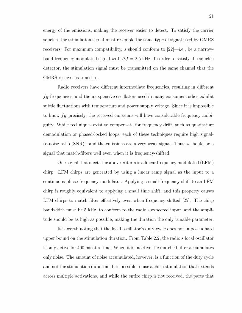
It is worth noting that the local oscillator’s duty cycle does not impose a hard
upper bound on the stimulation duration. From Table 2.2, the radio’s local oscillator
is only active for 400 ms at a time. When it is inactive the matched filter accumulates
only noise. The amount of noise accumulated, however, is a function of the duty cycle
and not the stimulation duration. It is possible to use a chirp stimulation that extends
across multiple activations, and while the entire chirp is not received, the parts that

22
are received still correlate. With the above in mind, our matched filter detector uses
a high-energy LFM chirp that is N = 216 samples long at its operating sampling rate
of 64 kHz, giving it a period of roughly 1024 ms. The stimulation signal is shown in
Figure 2.3.
The matched filter detector transmits this LFM chirp to the radio and applies
the matched filter to the received fH emissions. The matched filter is a finite impulse
response (FIR) filter, and thus it can be applied quickly using FFT techniques. Since
the matched filter detector, shown in Figure 2.7, knows that each chirp is N samples
long, it searches for a maximum of one match every N samples. The output is
then compared with a threshold detector: if the matched filter’s output exceeds the
threshold, a detection occurs. In order to determine how many chirps have been
received recently, an integrator counts the number of detections that have occurred
within the past few seconds.
2.3. THEORETICAL PERFORMANCE
Each detector’s theoretical performance was evaluated using artificial GMRS
radio emissions. Due to RF propagation, antenna, receiver sensitivity, and emissions
power differences, it is challenging to fairly compare these two algorithms in an ex-
perimental setting. The detectors use two different emissions frequencies, fLO and
fH , that radiate in a different fashion, with different power levels. This invariably re-
sults in different signal-to-noise ratios (SNR) at the receiver, giving one algorithm an
Streamto
Vector
N
|x|Magnitude
MatchedFilter Threshold
Max
N fs
N
Emissions Detection
Figure 2.7: A stimulated emissions detection algorithm using matched filters.
23
advantage over the other. To compare these detectors under equal-SNR conditions,
artificial emissions were generated based on experimental data.
2.3.1. Emulating GMRS Emissions. The emissions simulator generates
two sets of emissions: fLO emissions and fH emissions. The simulated fLO emissions
start as a constant-amplitude sine wave, and the fH emissions start as a perfect-
match LFM chirp. Both signals start with exactly identical RMS powers (0 dBW).
Prior to testing, the signals are time-limited, frequency-shifted, and corrupted with
additive white Gaussian noise.
GMRS radios have different local oscillator duty cycles when they are unstim-
ulated (state S0) and when they are stimulated (state S1). To emulate this effect,
the ideal emissions are multiplied with square waves with the same duty cycles that
are listed in Table 2.2. The square wave has a value of 1 when the LO is “on” and
0 when the LO is “off,” windowing the emissions in the time domain. Finally, the
emissions are subjected to channel effects.
The artificial emissions are corrupted with a small frequency shift and additive
noise. Since the exact emissions frequencies can never be known in advance, both
emissions are subjected to a small (1 kHz) linear frequency shift. After shifting the
emissions, both the fLO and the fH signals are corrupted by the exact same additive
white Gaussian noise sequence. The amount of noise was varied to produce SNRs
from 0 dB to −35 dB. The artificial emissions and the generated noise signal are
then saved for testing.
2.3.2. Quantitative Results. The artificial emissions were used to compare
the efficacy of both detectors in terms of their Receiver Operating Characteristic
(ROC) curves. To test the case where a radio is present, the artificial fLO emissions
were run through the periodogram detector, and the artificial fH emissions were run
through the matched filter detector. To test the case where no radio is present, both
detectors were run using the generated noise signal as input. Each true positive (ptrue),

24
false positive (pfalse), true negative (ntrue), and false negative (nfalse) was counted, and
the test was repeated for many different detector thresholds.
For each test, the false positive rate (fpr) and true positive rate (tpr) were
calculated as
fpr =pfalse
pfalse + ntrue
(2.7)
tpr =ptrue
ptrue + nfalse
(2.8)
When plotted, the false positive and true positive rates represent the ROC curve.
While both algorithms performed equally well for high SNRs, the difference became
more pronounced at lower SNRs.
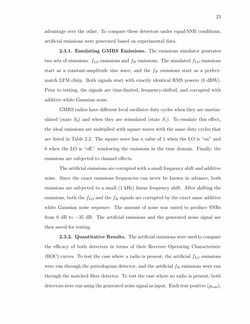
Figure 2.8 shows the ROC curves for both detectors for various signal-to-noise
ratios. Since the matched filter detector has more area under each curve than the
periodogram detector, it more accurately determines whether or not a radio is present.
Since the matched filter detector outperforms the periodogram detector under high-
noise conditions, the stimulated emissions approach is a quantitative improvement
over existing algorithms for detecting radio receivers.
It may be possible to further improve the performance of both the active and
passive detectors. Wavelets are widely used in chirp radar applications [26], and
their high time/frequency resolution may assist in the location of radio receivers.
Additionally, new statistical techniques can increase the sensitivity of periodogram
detectors. By comparing the periodogram with a probability distribution, rather
than a threshold, it is possible to reliably determine if a sinusoidal signal is present—
without the need to set a threshold [27].
2.3.3. Qualitative Results. In addition to the quantitative gains, the
matched filter detector offers a qualitative reduction in false positives. High-frequency
oscillators are not unique to radio receivers. Many other types of circuits—such as
25
0
0.2
0.4
0.6
0.8
1
0 0.2 0.4 0.6 0.8 1
Tru
eP
osit
ive
Rat
e
False Positive Rate
ROC: Matched Filter Detector with Simulated Noise
-25 dB (area 1.00)-30 dB (area 0.96)-35 dB (area 0.54)
≥ -25 dB-30 dB
-35 dB
(a) Matched Filter Detector
0
0.2
0.4
0.6
0.8
1
0 0.2 0.4 0.6 0.8 1
Tru
eP
osit
ive
Rat
e
False Positive Rate
ROC: Periodogram Detector with Simulated Noise
-20 dB (area 1.00)-25 dB (area 0.84)-30 dB (area 0.52)
≥ -20 dB
-25 dB
-30 dB
(b) Periodogram Detector
Figure 2.8: Receiver Operating Characteristics of both the matched filter detectorand the periodogram detector. The matched filter detector significantlyoutperforms the periodogram detector when the signal-to-noise ratio is−25 dB or less.
26
digital logic systems—may incorporate them. If such a device has high frequency
emissions near fLO, then it may cause a false positive on a periodogram detector.
Conversely, the matched filter detector provides assurances that the detected device
is a superheterodyne receiver, since only a superheterodyne receiver will react to the
stimulation as shown here. For applications that depend on the reliable detection of
radio receivers in the presence of other electronics, the stimulated emissions approach
is clearly superior.
2.4. CONCLUSION
The proposed stimulated emissions approach outperforms existing methods for
detecting superheterodyne receivers. Measurements of unintended emissions demon-
strate that two-way superheterodyne radios have higher-energy emissions when stim-
ulated, facilitating accurate detection. Key emissions are shown to have an identical
complex envelope to the stimulation signal, making it possible to detect receivers
using a matched filter. Theoretical performance testing affirms that, under low SNR
conditions, the matched filter detector offers a 5–10 dB performance gain over passive
techniques. While an experimental performance evaluation is necessary, these results
indicate that the stimulated emissions approach is a useful technique for reliably
detecting superheterodyne radio receivers.

27
3. LOCATING SUPERHETERODYNE RECEIVERS
As the preceding sections demonstrate, one strategy for mitigating explosive
threats is to detect radio receivers. Previous work has shown that radio receivers
have unintended electromagnetic emissions [15,16]. These unintended radio frequency
(RF) emissions are present any time the receiver is powered on and cannot be easily
eliminated with shielding. They are, however, limited in power and may be masked by
stronger signals from intentional radiators, making them difficult to detect. In many
cases, it is possible to improve detection by using stimulated emissions techniques.
Stimulated emissions is a well-known phenomenon [14,17] that can occur in a
variety of electronic devices. Certain types of devices—most notably, radio receivers—
are inherently sensitive to ambient RF signals. By transmitting a weak stimulation
signal, it is possible to alter the internal state of the device. The change in state causes
a change in the device’s unintended emissions. A stimulated emissions detector, such
as the one depicted in Figure 3.1, can offer improved sensitivity and selectivity over
passive detectors [12], since detection uses specific information about the emissions.
For the sake of clarity, the superheterodyne receiver that the system is attempting to
locate is referred to herein as the target device.
Knowing the position of the target device, as well as whether or not the
device is moving, would help confirm the presence of an explosive threat. The system
developed in [12] to detect radio receivers is merely a proximity detector. It can detect
the presence of a target device, but it cannot determine its location. RF sources can
be located by measuring the received signal strength, angle of arrival (AoA), or time
of arrival (ToA) of the radio signal. Any of these techniques can be applied to locate
unintentional radiators.

28
Received-signal-strength and angle-of-arrival algorithms are ill-suited to this
particular application. Received-signal-strength methods make the implicit assump-
tion that the source signal radiates isotropically [28]. This assumption does not hold
for unintended emissions, which do not have purpose-built isotropic antennas. Angle-
of-arrival techniques require directional antennas [29] or large antenna arrays [30],
which increase the size and expense of the system. Subspace techniques such as Es-
timation of Signal Parameters Via Rotational Invariance Techniques (ESPRIT) offer
high-resolution AoA estimation [31], but they are seldom realized in hardware and
are particularly sensitive to multipath [32].
ToA techniques are frequently used in radar and radio-navigation systems. In
the Global Positioning System (GPS), receivers determine their position by measuring
the ToA of synchronized signals from multiple sources [33]. This technique is known
as time difference of arrival (TDoA). The accuracy of these radio-navigation systems
is dependent, in part, on the accuracy of the TDoA measurements. In order to be of
practical use, a radio receiver locator must make highly accurate ToA measurements.
TargetDevice
Detector(USRP)
Stimulation
Emissions
Tx
Rx
467 MHz
908 MHz
Figure 3.1: The stimulated emissions detection process. A stimulated emissions de-tector alters the unintended emissions in a predictable manner. Themodified emissions radiate back into the environment, where they aredetected. The frequencies given above are an example only.

29
A ToA-based method is developed in the following paper for determining the
range to non-cooperative radio receivers using stimulated emissions. The method
extends the previous stimulated detection approach, which could not locate radio
receivers, to allow ToA measurement. The theoretical accuracy of the ToA estimates
is determined using near-field measurements. A radar-like technique is used to lo-
cate consumer radio receivers in a real RF propagation environment. Experimental
performance tests indicate that it is possible to reliably and accurately locate super-
heterodyne receivers.
3.1. METHODS
The crucial factor impacting the accuracy of a time-of-arrival estimation sys-
tem is, as the subsequent sections will demonstrate, the available bandwidth. Ex-
isting stimulated emissions techniques, which are briefly reviewed, do not take the
bandwidth limitations of the target device into account. The bandwidth of a Gen-
eral Mobile Radio Service receiver is measured, and an appropriate time-of-arrival
technique is developed based on the characteristics of the stimulated emissions. The
hardware implementation of this technique, which is based on chirp radar, is also
discussed.
3.1.1. Wideband Stimulated Emissions. In [12], it was demonstrated
that superheterodyne receivers have stimulated emissions that are a frequency-trans-
lated copy of the stimulation signal. Superheterodyne receivers, such as the one shown
in Figure 3.2, use mixers to perform frequency translation [34]. In this receiver, the
RF signal is shifted in frequency to a fixed intermediate frequency, fIF , by selecting
the local oscillator frequency, fLO, such that
fIF = fRF − fLO. (3.1)

30
By the modulation theorem, the mixer also creates an up-mixing component,
fH , at
fH = fRF + fLO. (3.2)
It has been shown that superheterodyne receivers can be detected by transmitting
an arbitrary stimulation signal at fRF and searching for the fH emissions with a
correlator. In order to locate the receiver, the round-trip time of the stimulated
emissions must also be accurately measured.
Others have shown that the accuracy of time-of-arrival measurements depends
on the signal-to-noise ratio (SNR) and waveform of the received signal [35]. While
it is difficult to obtain a closed-form expression of accuracy for arbitrary signals,
closed-form solutions for specific radar signals exist. As given in [35], the accuracy of
a linear, frequency-modulated (LFM) chirp is
δRideal =c√
3
2πB(2E/N0)1/2, (3.3)
fRF
IF Filter
fIF
ImageRejection
Filter RF Mixer
Local Oscillator
fLO
fHRadiated
Emissions
Figure 3.2: A superheterodyne front-end which uses low-side injection. The radiatedemissions originate from the RF mixer.

31
where δRideal is the root mean square (RMS) position error, c is the speed of light,
B is the chirp bandwidth, and E/N0 is the SNR in linear units. The RMS error
represents the average-case, absolute position error.
From (3.3), the error δRideal decreases proportionally with respect to the band-
width used—but only with the square root of the SNR. This property makes it highly
advantageous to use wideband signals for time of arrival-based location. The narrow-
band, B = 5 kHz chirps used in [12] have an error that is too large to be of practical
use for realistic SNRs. Additional bandwidth is required to perform meaningful time
of arrival-based location.
While superheterodyne receivers were previously detected using narrowband
stimulations, which were the width of a single voice channel, superheterodyne front-
ends are sensitive to a much wider range of frequencies. Consider the simplified
receiver front-end in Figure 3.2. The mixer, which produces the fH stimulated emis-
sions, must be sensitive to the entire range of frequencies to which the radio can tune.
The bandwidth of the signal that can enter the mixer is limited only by the resonance
of the antenna and the image rejection filter.
The image rejection filter is designed to eliminate frequencies which are far
outside of the receiver’s tuning range. Superheterodyne receivers select two channels
at once, making it necessary to eliminate one of them with a filter. The unwanted
channel, known as the image frequency, is located at
fimage = fRF − 2fIF (3.4)
for low-side injection receivers. For receivers using the popular fIF = 21 MHz in-
termediate frequency, the image frequency is 2fIF = 42 MHz away from the RF
channel. Since the frequency separation is relatively large, the image rejection filter

32
can—but does not necessarily—have a pass band that is much wider than the range
of frequencies to which the device can tune.
Receivers that use such image rejection filters, with wider-than-necessary pass
bands, can have a stimulated emission’s bandwidth which far exceeds their tuning
range. This theory is important, as higher bandwidths yield more precise position
measurements. In order to determine the usable bandwidth of real-world devices, a
number of consumer superheterodyne receivers were selected for testing in a controlled
environment.
3.1.2. Bandwidth Measurements. Initial testing was performed using
General Mobile Radio Service (GMRS) radios. GMRS radios are typical consumer
superheterodyne receivers. GMRS is a low-power land-mobile radio service, which
operates on frequencies in the 460 MHz range using analog frequency modulation.
Since superheterodyne radio receivers have been available for many years [36, 37],
most commercially-available radio receivers use very similar designs, and results with
the tested receivers are easily generalizable to other devices and services.
The stimulated emissions bandwidth that can be used with a GMRS receiver
was determined using frequency-domain measurements. While a superheterodyne
receiver is not a strictly linear system, the principal non-linearity—the mixer’s fre-
quency shift—is known from (3.2). By transmitting a stimulation signal on fRF and
measuring the corresponding stimulated emissions on fH , it is possible to determine
the linearized system’s frequency response. To improve isolation from ambient RF
signals, these measurements were conducted in an enclosed near-field environment.
A GMRS receiver was placed in a transverse electromagnetic (TEM) cell, and
its stimulated response was measured. The device under test was a double-conversion
superheterodyne receiver with an intermediate frequency of fIF = 21.4 MHz. The
stimulated response was determined using a swept-sine technique similar to that

33
in [38]. A signal generator was used to produce a swept sinusoidal stimulation from
450 – 560 MHz. The stimulated emissions were measured using a spectrum analyzer.
The stimulated response is shown in Figure 3.3. The results indicate that the
GMRS receiver will generate stimulated emissions over a bandwidth of approximately
16 MHz. This measurement is significant since the GMRS receiver is only designed
to receive a 175 kHz-wide band. The receiver’s response is dominated by the pass-
band properties of the image rejection filter. The emissions are within 3 dB of the
peak power for stimulation frequencies of 455.853 MHz – 478.893 MHz. Outside of
this band, the image rejection filter attenuates the stimulation signal, limiting the
bandwidth of the emissions.
Results show that sufficient bandwidth exists for high-resolution location. Al-
though sufficient bandwidth is available, other factors may impact or impede far-field
distance measurements.
-80
-75
-70
-65
-60
-55
-50
-45
-40
440 460 480 500 520 540 560 580
Em
issi
ons
Pow
er(d
B)
Stimulation Frequency (MHz)
Bandwidth of GMRS Stimulated Emissions
Figure 3.3: Stimulated emissions of a GMRS receiver. The 3 dB bandwidth, mea-sured relative to the power at GMRS channel four (462.6375 MHz) isindicated on the plot as a dashed line.

34
3.1.3. Time of Arrival Method. Continuous-wave radar concepts can be
applied to locate radio receivers. Pulse-radar techniques would not work well since
superheterodyne receivers frequently incorporate low-noise amplifiers which compress
the dynamic range of the received signal and, by extension, the stimulated emissions
[39]. Signals with nearly-constant power, such as continuous-wave signals, can deliver
a higher average power through these amplifiers [40].
Frequency-modulated continuous wave (FMCW) radar methods are well-suited
to detecting superheterodyne receivers. FMCW radar uses a swept-sine signal to
achieve the bandwidth required for accurate ranging. Although a variety of FMCW
signals have been studied, efficient techniques exist for processing linear FM chirps.
As described in [41, 42], and elsewhere, delaying an LFM chirp in time is equivalent
to shifting it in frequency. The difference between the transmitted frequency and the
received frequency determines the range information.
The frequency difference, which is often referred to as the beat frequency, is
given by the relationship
fb =τB
T, (3.5)
where fb is the beat frequency, τ is the time delay, and T is the chirp period [41].
This relationship makes it possible to implement FMCW radar using mixers. In order
to determine the beat frequency, the received echoes are mixed with the complex
conjugate of the transmitted chirp signal. The product signal contains, among other
periodic terms, the beat frequency signal. This reduces the range estimation problem
to a frequency estimation problem.
The Fast Fourier Transform (FFT) is a numerically efficient estimate of the
beat frequency. A one-dimensional FFT estimates range, and a two-dimensional FFT
estimates range and doppler shift simultaneously [40,43]. FFTs from successive chirp
periods are typically averaged together using periodogram techniques. Due to the

35
oscillator drift between the radar and the target device, the “doppler” frequency has
a different meaning in this application compared to traditional radar.
The major difference between conventional radar and the technique used here
is that the return signal is not a reflection; it is modified emissions from the target
device. Traditional radar has a strictly linear echo path, and any frequency shift
is the result of the doppler effect. This is not the case for stimulated emissions,
which are shifted in frequency by the target device’s local oscillator. In practice, the
local oscillator frequency is unknown and may drift somewhat over time. The precise
stimulated emissions frequency is, by extension, unknown, but it can be estimated
using doppler processing techniques.
Doppler shift is usually modeled as a linear frequency shift between the trans-
mitted and received radar signals [44]. Techniques for estimating doppler can thus
estimate the frequency shift between the radar and the target device. This estimate
is useful for separating multiple targets, which tend to have slightly different local
oscillator (LO) frequencies. The “doppler” estimate is also necessary to ensure that
the mutual oscillator drift between the radar and the target device does not result in
range ambiguity.
Due to the relationship between a time shift and a chirp frequency shift, ex-
cessive frequency shift will also change the estimated range. From [40], the maximum
unambiguous frequency shift ∆D is
∆D =1
T. (3.6)
If either the radar’s oscillator or the target’s oscillator drift in frequency by more
than ∆D, the estimated range will change. While longer chirps are preferable, since
they deliver more energy per chirp, the chirp period T must be small enough to avoid
this ambiguity.

36
The mixer implementation quantizes all range estimates into discrete range
bins. As derived in [45], the range resolution for frequency-modulated sawtooth
waveforms is
∆R ≈ Tc
2B
√(1
T − td
)2
+ ∆f 2r , (3.7)
where td is the transition time between chirps, and ∆fr is the frequency resolution of
the receiver. Assuming a sufficiently fine-grained frequency estimate (∆fr = 0) and
instantaneous transitions (td = 0), this simplifies to
∆R ≈ c
2B. (3.8)
The size of the range bins is thus a function of bandwidth. With B = 16 MHz of
bandwidth, each range bin is ∆R ≈ 9.4 m wide.
3.1.4. Hardware Realization. The radio receiver’s near-field bandwidth
is not, by itself, sufficient to determine the performance of a ToA range estimation
system. RF propagation, such as antenna resonance and multipath, can have a sub-
stantial impact on the stimulated emissions in the far-field. Oscillator imperfections
can result in frequency drift and phase noise, reducing resolution [40]. To test the
effects of these factors, a continuous-wave radar was designed and implemented in
hardware.
An FMCW radar-like system was designed to implement the stimulated emis-
sions process described in Figure 3.1 and in the last section. Existing FMCW radars
are designed to detect linear echoes from reflective surfaces. They are ill-suited for
detecting unintended emissions, which may have very different stimulation and emis-
sions frequencies (fRF 6= fH). This design requirement necessitates the development
of a modified FMCW radar with greater frequency agility.
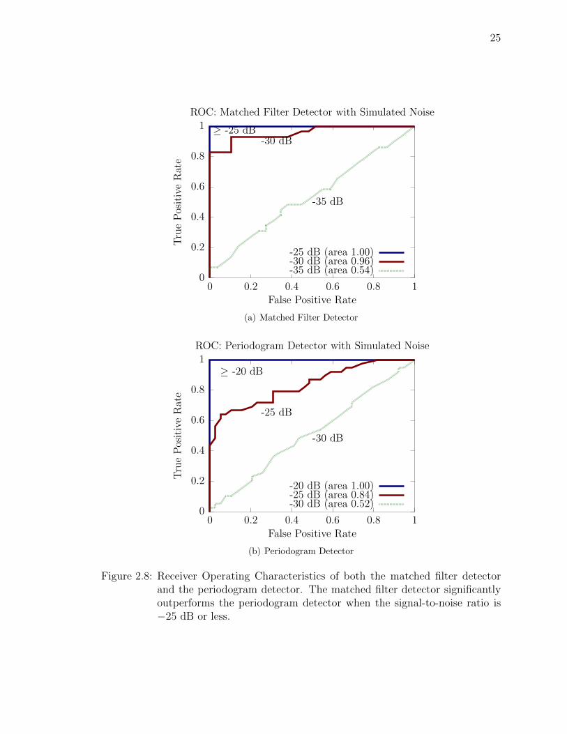
The stimulated emissions radar uses a Universal Software Radio Peripheral
(USRP) to perform high-speed signal processing. The USRP is a software-defined
37
radio that enables personal computers (PC) to transmit and receive radio signals. A
block diagram of the radar system is presented in Figure 3.4. Additional information
about the USRP system and software-defined radio in general is given in Appendix 5.
The USRP incorporates two independently-tuned daughtercards for RF fron-
tends. One card transmits the stimulation signal at fRF, and the other receives the
fH stimulated emissions. The receiver uses a yagi antenna for extra directionality,
additional analog filtering to attenuate the transmitted signal, and external low-noise
amplifiers to increase the SNR. The USRP’s field-programmable gate array (FPGA)
performs the high-speed radio and radar signal processing.
The USRP connects to its host PC through the Universal Serial Bus (USB)
protocol. This connection has a maximum transfer rate of 8 MSa/s [21], which is
too slow to accommodate wideband chirp radar signals and satisfy real-time perfor-
mance requirements. To reduce the required throughput, a custom FPGA bitstream
performs the chirp and de-chirp operations. The radar frontend uses a sawtooth
waveform with an adjustable period and bandwidth.
The beat frequency signal is filtered, decimated, and transferred to the host
PC. The resulting signal has an integer number of samples per chirp, N . A range-
Doppler periodogram, similar to that in [43,46], estimates range and frequency shift.
TransmitterHardware
(daughter-card)
RxAnt.
TxAnt.
Chirp Gen.ReceiverHardware
(daughter-card)
conj
Band-Pass
Local Osc.
USB
FFT2
Range-Doppler
Processor
Universal Software Radio Peripheral
Time
Fre
q
Low-Pass
+28 dB
LNA
TargetDevice
Figure 3.4: Hardware realization of the stimulated emissions radar. A linear FM chirpgenerator was added to the USRP’s FPGA. The de-chirped emissions aredown-mixed, decimated, and output to the host PC for further processing.

38
To compute the periodogram, N chirps are accumulated, as column vectors, into an
N × N matrix. A Hamming window is applied to the matrix to reduce the effects
of the inter-chirp transitions. The two-dimensional FFT (2N × 2N points) of the
matrix is computed.
Multiple FFTs are averaged together, forming a two-dimensional range-doppler
periodogram [47]. The target’s range and frequency shift are estimated from the max-
imum of the periodogram. While more advanced frequency estimation [48] and track-
ing techniques are available, this estimate suffices for single-device tests. A simple
post-processor improves the effectiveness of the range-doppler processor.
The RF front-end of the USRP used in these experiments is less than ideal
for FMCW radar. Even with extra analog filtering, there is strong, in-system cou-
pling between the transmitted stimulation and the received emissions. The coupling
increases the received power of several different doppler frequencies. These spuri-
ous bands of energy make it necessary to estimate the noise floor of each doppler
frequency individually.
The post-processor estimates the noise floor of each doppler frequency using its
20-quantile power—i.e., the power that only 20% of the cells are less than. The noise
estimates are then used to equalize the power of all doppler shifts. This technique is
a simple form of the constant false-alarm rate (CFAR) processor which is commonly
used in radar systems [49].
The accuracy of the radar system was verified by using a long coaxial cable
as a delay line. The radar transmitter was connected directly to the receiver via a
34.3 meter RG-58 cable. A frequency doubler was placed in the loop to mimic the
frequency shift which occurs in a superheterodyne mixer. The radar made thirty
range estimates over a 2.5 minute period, using both 16 MHz and 32 MHz of band-
width. No drift or variance was observed in the range estimates. The USRP’s range
estimates (48.8 m) are reasonable given both its resolution and the velocity factor of

39
the coax. After validation testing, the stimulated emissions radar was used to locate
superheterodyne receivers.
3.2. RESULTS
Field trials of the stimulated emissions radar were conducted using two differ-
ent target devices at two different locations. The first device was the GMRS receiver
from Section 3.1.2, which had approximately 16 MHz of usable bandwidth. The sec-
ond device was a wideband radio scanner which had a tuning range of 420 – 470 MHz
(> 50 MHz bandwidth). Both devices were commercially-available superheterodyne
receivers that were certified to comply with FCC radiated emissions limits. The
GMRS receiver is a typical low-cost consumer receiver, while the wideband scanner
is a higher-quality, more sensitive device. The range to these devices was determined
using the USRP as previously described.
The chirp parameters were chosen such that the stimulated emissions band-
width was identical for both devices. From Figure 3.3, a B = 16 MHz-wide chirp
centered on fRF = 467 MHz will pass through the GMRS receiver. Two different
tests, one outdoors and the other indoors, were conducted for each target device.
Both tests used similar hardware configurations and an identical test procedure.
During each trial, the target device was carried by hand on a fixed path,
first away from and then towards the radar unit. The target was kept in motion
continuously during each trial, with an average velocity which varied from 0.85 m/s
to 1.07 m/s.
In order to increase the SNR, the target device’s squelch detector (see [12])
was disabled, forcing the receiver to be active continuously. The stimulated emissions
radar tracked and estimated the range to the target device throughout the trial. A
chirp period of T = 0.8 ms was chosen to allow for ∆D = 1.25 kHz of unambiguous
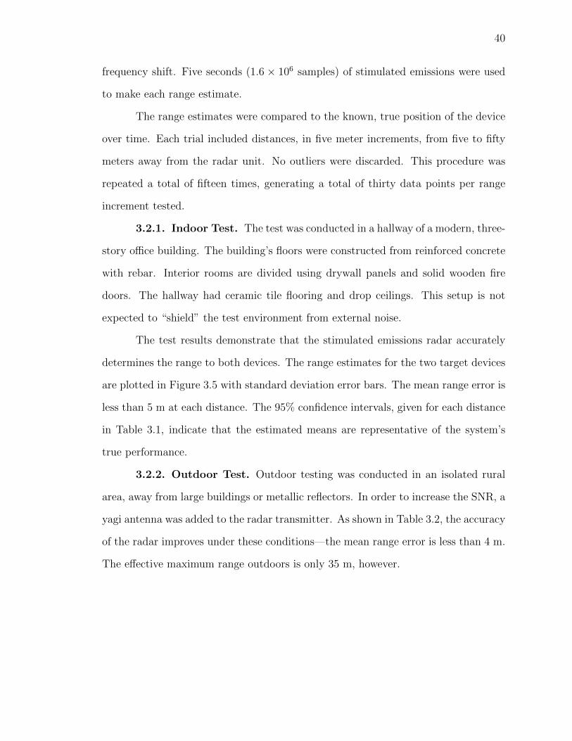
40
frequency shift. Five seconds (1.6 × 10⁶ samples) of stimulated emissions were used
to make each range estimate.
The range estimates were compared to the known, true position of the device
over time. Each trial included distances, in five meter increments, from five to fifty
meters away from the radar unit. No outliers were discarded. This procedure was
repeated a total of fifteen times, generating a total of thirty data points per range
increment tested.
3.2.1. Indoor Test. The test was conducted in a hallway of a modern, three-
story office building. The building’s floors were constructed from reinforced concrete
with rebar. Interior rooms are divided using drywall panels and solid wooden fire
doors. The hallway had ceramic tile flooring and drop ceilings. This setup is not
expected to “shield” the test environment from external noise.
The test results demonstrate that the stimulated emissions radar accurately
determines the range to both devices. The range estimates for the two target devices
are plotted in Figure 3.5 with standard deviation error bars. The mean range error is
less than 5 m at each distance. The 95% confidence intervals, given for each distance
in Table 3.1, indicate that the estimated means are representative of the system’s
true performance.
3.2.2. Outdoor Test. Outdoor testing was conducted in an isolated rural
area, away from large buildings or metallic reflectors. In order to increase the SNR, a
yagi antenna was added to the radar transmitter. As shown in Table 3.2, the accuracy
of the radar improves under these conditions—the mean range error is less than 4 m.
The effective maximum range outdoors is only 35 m, however.

41
Table 3.1: Indoor Test Results
Est. Range (m)
GMRS Scanner
Range (m) Mean 95% CI Mean 95% CI
5 3.0 0.6 5.0 1.4
10 10.7 1.3 9.8 0.5
15 12.5 0.8 15.5 1.3
20 23.3 1.6 22.3 1.1
25 24.4 1.5 27.0 1.2
30 30.5 0.8 30.8 1.3
35 33.3 1.7 34.6 1.8
40 40.2 0.6 45.0 1.9
45 48.0 1.3 49.5 1.0
50 49.7 0.5 49.7 1.4
Table 3.2: Outdoor Test Results
Est. Range (m)
GMRS Scanner
Range (m) Mean 95% CI Mean 95% CI
5 5.0 0.3 5.0 0.9
10 7.8 0.8 7.8 1.3
15 14.0 1.1 14.0 0.9
20 19.2 1.2 19.2 1.3
25 23.7 0.8 23.7 0.9
30 29.6 1.5 29.6 1.4
35 33.1 0.9 33.1 1.5
40 43.2 4.1 43.2 4.6

42
3.3. DISCUSSION
Wideband stimulated emissions is, demonstrably, an effective technique for
locating superheterodyne receivers. An analysis of the system’s accuracy, which is
given below, indicates that the system has a reasonable noise performance which
corresponds well to the theoretical model. While it is possible to locate radio receivers
using wideband stimulated emissions, a number of important challenges remain. The
target device introduces a number of limitations which can reduce the effectiveness
of the system. Multipath can also pose a problem, particularly indoors. These
0
10
20
30
40
50
60
0 10 20 30 40 50 60
Est
.R
ange
(m)
Range (m)
Range Estimates: GMRS Receiver
MeasuredTrue Range
0
10
20
30
40
50
60
0 10 20 30 40 50 60
Est
.R
ange
(m)
Range (m)
Range Estimates: Wideband Receiver
MeasuredTrue Range
Figure 3.5: Indoor range estimates of the GMRS receiver and the wideband scanner.Each range estimate plotted above is the mean of thirty range measure-ments; estimates are plotted with standard deviation error bars. The truerange is plotted, for reference, as a dashed line.
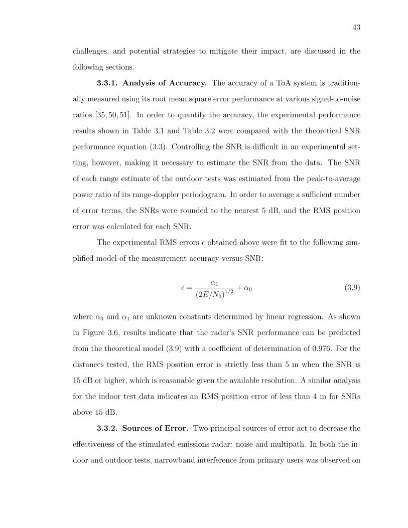
43
challenges, and potential strategies to mitigate their impact, are discussed in the
following sections.
3.3.1. Analysis of Accuracy. The accuracy of a ToA system is tradition-
ally measured using its root mean square error performance at various signal-to-noise
ratios [35, 50, 51]. In order to quantify the accuracy, the experimental performance
results shown in Table 3.1 and Table 3.2 were compared with the theoretical SNR
performance equation (3.3). Controlling the SNR is difficult in an experimental set-
ting, however, making it necessary to estimate the SNR from the data. The SNR
of each range estimate of the outdoor tests was estimated from the peak-to-average
power ratio of its range-doppler periodogram. In order to average a sufficient number
of error terms, the SNRs were rounded to the nearest 5 dB, and the RMS position
error was calculated for each SNR.
The experimental RMS errors ε obtained above were fit to the following sim-
plified model of the measurement accuracy versus SNR:
ε =α1
(2E/N0)1/2
+ α0 (3.9)
where α0 and α1 are unknown constants determined by linear regression. As shown
in Figure 3.6, results indicate that the radar’s SNR performance can be predicted
from the theoretical model (3.9) with a coefficient of determination of 0.976. For the
distances tested, the RMS position error is strictly less than 5 m when the SNR is
15 dB or higher, which is reasonable given the available resolution. A similar analysis
for the indoor test data indicates an RMS position error of less than 4 m for SNRs
above 15 dB.
3.3.2. Sources of Error. Two principal sources of error act to decrease the
effectiveness of the stimulated emissions radar: noise and multipath. In both the in-
door and outdoor tests, narrowband interference from primary users was observed on

44
both the stimulation and emissions frequencies. Substantial noise also originates from
the radar transmitter and couples, via the USRP board, directly into the receiver.
Although the impact of these noise sources is reduced by the spread-spectrum radar
signal and the post-processor, respectively, they still decrease the dynamic range of
the radar. Others have shown that the noise power tends to be higher outdoors [52],
and this reduced the outdoor range and noise performance. A more sensitive front-
end, with automatic gain control and a higher sampling depth, could increase the
radar’s effective range.
Multipath can cause false targets and inaccurate distance measurements, and
the effect can be severe in indoor environments. Others have conducted extensive
studies of indoor multipath in real environments. Measurements conducted in an
office building indicate that the multipath delay within a single room can exceed
100 ns, with a root mean square (RMS) delay spread of 50 ns [53]. Since each
0
5
10
15
20
25
30
35
0 10 20 30 40 50
RM
SE
rror
(m)
Estimated SNR (dB)
Noise Performance of USRP Radar
Figure 3.6: Root mean square error performance of the stimulated emissions radar.This plot includes all measurements, for both target devices, from theoutdoor test. Each data point contains at least forty observations. Thefit with the theoretical model (3.9) is plotted as a dashed line.

45
FMCW radar bin only differs by 15 ns, multipath can easily affect the results. Strong
multipath negatively impacted the accuracy of the radar during the indoor tests.
Techniques for reducing the effects of multipath and non-line-of-sight propagation
are a crucial area of future development.
3.3.3. Device Limitations. Design differences between superheterodyne re-
ceivers make it difficult, but not impossible, to determine the absolute range. The tar-
get device imposes its own delay on the stimulated emissions as they pass through the
superheterodyne front-end. This delay, while imperceptible to the user, may nonethe-
less differ from device to device. The GMRS receiver and the wideband receiver used
in this experiment have delays which differ by 94 ns, which is approximately 3∆R.
This difference is too large to measure the absolute range to an unknown device, but
the relative range estimates can still be used for two-dimensional positioning.
Time difference of arrival combines relative range estimates, taken from mul-
tiple sensors, into a two or three-dimensional position fix. Such techniques have been
applied to locate devices in both line-of-sight [50] and non-line-of-sight [51] condi-
tions. The accuracy of TDoA depends solely on the array geometry and the accuracy
of each time of arrival measurement [54]. The performance measurements collected
in this study could, in future work, be used to estimate the performance of a TDoA
stimulated emissions locator.
3.4. CONCLUSION
The proposed wideband stimulated emissions technique can determine the
range, using time-of-arrival measurements, to a superheterodyne receiver. Measure-
ments conducted with a continuous-wave radar unit demonstrate that this technique
can locate commercially-available superheterodyne receivers. The radar achieved a
root mean square position error of less than five meters outdoors, and four meters

46
indoors, at 15 dB SNR or higher. The system is capable of functioning in non-ideal
propagation environments with multipath and narrowband interference sources.
Although the system presented in this study can only measure the relative
range to the device, the ability to make such measurements is crucial to the de-
velopment of a true position-finding system. Extending the stimulated emissions
radar to operate in two dimensions, using time difference of arrival, is a relatively
straightforward task with well-characterized performance. The performance of this
technique is limited chiefly by the available bandwidth. When applied to modern,
high-bandwidth communications systems, stimulated emissions has the potential to
enable high-precision indoor location—even when the target device does not intend
to be found.

47
4. DETECTING AND IDENTIFYING MICROCONTROLLERS
Clocked digital systems become more and more ubiquitous with each passing
year. The market for low-end microcontrollers, which can replace costly application-
specific integrated circuits and discrete components, continues to grow. Many prod-
ucts which contain microcontrollers, including garage door openers and passive in-
frared sensors, can be used to initiate explosive devices [11]. The detection and iden-
tification of microcontrollers can therefore aid in the screening for and the evaluation
of explosive threats.
Electronic devices can be detected using their unintended electromagnetic
emissions. Any high-frequency signal, including those generated from clocks, I/O
lines, and internal switching, can radiate into the environment as electromagnetic
emissions. Microcontrollers can be responsible for a significant portion of a printed
circuit boards’ (PCB) emissions [55]. As such, they are one of the more readily-
detectable components in a digital device.
Under typical operating conditions, however, microcontroller emissions are
not the only signal that is present in the environment. A great number of radio-
frequency (RF) emitters, both intentional and unintentional, exist in the band from
1 MHz – 600 MHz where microcontroller emissions tend to occur. A selective detector
should be able to distinguish microcontroller emissions from sinusoidal signals, such
as the radio receiver local oscillators in [12] and communications signals like frequency
modulation (FM). In order to detect unknown devices, few assumptions can be made
about the pulse shape, frequency, or jitter.
Antenna arrays offer many promising results for separating signals, but they
are only part of the solution. Array processing includes spatial techniques such as
beamforming [56] and blind techniques such as independent component analysis [57].

48
Wiener filtering can also attenuate signals from distant sources [58]. While these
techniques may be useful for reducing the interference caused by high-power, in-
tentional radio transmitters, they are less useful for identifying the type of signal
being radiated. Positively identifying microcontroller emissions requires some type
of classification algorithm.
Classifying devices by their unintended emissions is a well-studied topic, and
many solutions exist. Others have developed techniques for identifying super-regen-
erative receivers [17], and previous work has shown that superheterodyne receivers
can also be identified [12]. Both of these techniques use an RF stimulation signal to
alter the device’s unintended emissions.
Microcontrollers, however, are designed to resist ambient RF signals. Others
have shown that altering the emissions of a digital device requires a prohibitively-
strong electric field [59]. The stimulated detection approach from [12] cannot be
applied here, but similar modeling and simulation techniques can be used to develop
passive classification algorithms. An accurate model requires an understanding of
where the electromagnetic emissions originate.
Microcontrollers have emissions which depend on the device’s current draw.
The current which flows through a microcontroller’s package can form a loop, induc-
tively driving the PCB and attached cables to radiate electromagnetic emissions [60].
In a synchronous, clock-driven processor, the vast majority of transistor switching oc-
curs at clock edges. This results in large current spikes during each clock cycle [61].
The emissions of most microcontrollers are thus expected to be highly impulsive and
dependent on the device’s clock, which is typically periodic. Many different clock
frequencies and resonator types are in use, however, and a generalized detection ap-
proach is required in order to detect different types of microcontrollers.
The following paper compares different methods for detecting the electromag-
netic emissions of digital clock circuits. An analytic model of these clock emissions is

49
developed and validated using measurements of an 8051 microcontroller. This model
is used, in a simulated environment, to evaluate the noise performance of several ex-
isting algorithms: the harmogram, the harmonic product spectrum, the fast folding
algorithm, and linear prediction. A novel detection algorithm, the harmogrant, is
proposed which uses pitch estimation with application-specific heuristics. The appli-
cability and usefulness of each algorithm as a clock-circuit detector is considered.
4.1. METHODS
The electromagnetic emissions of microcontrollers are known to be current-
dependent. If a model for the current draw at each clock cycle can be derived, it
may be possible to search for the presence of microcontrollers using model-fitting
techniques. Computer simulations of microcontroller current have been developed
[55], but these simulations can only generate data from known model parameters. A
simpler, analytic model is desirable not just for simulations, but for model-fitting as
well. Several methods for modeling and predicting the emissions are presented in the
following sections.
4.1.1. Autoregressive Model and Detector. An accurate, two-parameter
model exists for the current draw in complementary metal oxide semiconductor
(CMOS) devices. This model can be used both to simulate clock emissions and
to detect them. In most digital systems, the vast majority of transistor switching
occurs at the rising edge of the clock. This switching causes a substantial spike in the
device’s instantaneous current consumption. In [62], it was demonstrated that the
current draw at the clock transition can be modeled as an exponential rise followed
by an exponential decay.
The double-exponential model has two parameters: the damping ratio ξ and
the natural frequency ω. These parameters can be derived from measurable RLC

50
properties of the device in question. As given in [62], the unit step response for the
overdamped case (ξ > 1) is:
ic(t) =(e−(ξ−
√ξ2−1)ωt − e−(ξ+
√ξ2−1)ωt
)u(t). (4.1)
Each clock cycle, the current draw of the CMOS system is approximated by exciting
the system given in (4.1) with an impulse. This results in a periodic train of dampened
pulses. An example pulse train, with typical parameters, is given in Figure 4.1. This
current signal can drive unintended emissions.
Traditionally, pulse signals are detected using matched filters; this approach
is common in radar systems. The performance of a matched filter has been shown to
depend on the time-bandwidth product of the candidate signal [24]. The clock pulses
are already very sparse in time, which limits the effectiveness of such filters.
0 0.5 1 1.5 2 2.5 3 3.5 4
Cu
rren
t(A
mp
s)
Time (periods)
Simulated CMOS Clock Pulses
Figure 4.1: The current draw of a CMOS device. The current draw has an exponentialrise and an exponential decay. The pulses shown above have ξ = 1.093and ω = 1.22 GHz, which were taken from a real CMOS device in [1].
51
More importantly, matched filters require substantial a priori knowledge of
the signal’s characteristics [16]. The shape of the clock emissions is not known and
may vary from pulse to pulse, necessitating a large matched filter bank of candidate
signals. Model-fitting techniques can offer lower computational complexity, but fitting
arbitrary functions like (4.1) to received emissions is difficult. By reformulating the
problem as a linear-time invariant filter, a simpler solution emerges.
Taking the Z-transform of (4.1) with a sampling period of Ts, it is shown that:
Ic(z) =β1z
−1
1− e2α√
ξ2−1+1
eα(ξ+
√ξ2−1)
z−1 + e−2αξz−2(4.2)
where α = Tsω and β1 is a constant which depends on α and ξ. The filter Ic(z)
is an infinite impulse response filter with two feedback taps and one feed-forward
tap. If given an impulse train at the clock frequency as the input, it will produce an
approximation of the microcontroller’s current emissions. By inspection, Ic(z) only
has zeros at z =∞. Similar results hold for the under-damped and critically-damped
cases.
The feed-forward taps only represent a single-sample delay and attenuation of
the input. Since neither of these affect the overall pulse shape, and the time offset is
unknown to begin with, an equivalent filter is
Ic(z) =1
1− e2α√
ξ2−1+1
eα(ξ+
√ξ2−1)
z−1 + e−2αξz−2. (4.3)
This is an all-pole filter which applies to the under-, over- and critically-damped
cases, enabling it to handle emissions from devices with any damping ratio.
Although the current signal in (4.1) drives the electromagnetic emissions, the
received signal may not have the same form. The voltage received by a loop probe
and driving an inductively coupled antenna, for example, is proportional to the first

52
derivative of the current. For the over-damped case, this is not an issue, as the
current signal (4.1) is composed entirely of exponentials of the form eKt, where K is
a constant.
Since ddt
{eKt}
= KeKt, the derivative of i′c(t) has the same form—with the
exception of some constants—as ic(t). The same holds for higher-order derivatives as
well. Since the functions have the same form, the autoregressive model will have the
same order regardless of which derivative the antenna receives. The autoregressive
model is thus an appropriate fit for received electromagnetic emissions.
If the microcontroller emissions are assumed to be corrupted by additive white
Gaussian noise, then the overall system is an autoregressive process with two taps
(AR(2)). Linear prediction can be used to fit such an autoregressive model to received
data. This feature makes the AR model useful as a detector.
An autoregressive process, which is depicted in Figure 4.2, can be estimated
using linear prediction. In an AR process, an unknown excitation e is filtered with
an all-pole filtesr 1/A(z). The filtered signal x, which has been corrupted with white
noise, is observed. The goal of linear prediction is to estimate the all-zero filter
A(z) needed to undo (i.e., inverse filter) the unknown, all-pole system filter. Linear
prediction is often used in speech codecs [63].
Let a = A(z) be the system filter taps, which are a polynomial in z, and a
be the estimate of those taps. Since the all-zero filter has a finite impulse response
1A(z) Â(z)e ê
xc
WhiteNoise
ν
Figure 4.2: An autoregressive process. The goal of linear prediction is to estimatethe taps of the all-pole filter 1/A(z).

53
(FIR), it can be evaluated with convolution. As formulated in [64] and elsewhere,
the output after applying the estimated filter is
e = x~ a (4.4)
= Xa, (4.5)
where x is the received signal and X is its convolution matrix.
The excitation signal of the filter, e, is the portion of the signal which cannot
be predicted by the linear filter. It is therefore assumed to be small. The problem
then becomes one of minimizing the residuals e, which from (4.5) is equivalent to
mina||Xa||p subject to a0 = 1, (4.6)
where || · ||p denotes the Lp norm. The constraint avoids estimating a filter of a = 0.
Numerically-efficient solutions, such as Yule-Walker and the Burg method,
exist for the L2 norm [64]. By measuring the power of the residual signal e, it is
possible to determine how well the system fits an autoregressive model: lower power
indicates a better fit. Residual power is commonly used in information theory metrics,
such as Minimum Description Length, to measure goodness-of-fit [65,66].
In order to detect microcontroller clocks, the received unintended emissions
are fit to an AR(2) model using the Burg method. The power difference between the
input signal and the residuals is measured as
var(x)− var(e) = Ex
{x2}− E2
x {x} −(Ee
{e2}− E2
e {e}), (4.7)
where Ek{·} denotes the expectation function with respect to k. A detection occurs
if (4.7) rises above a certain threshold. Several other algorithms are commonly used

54
to detect periodic signals: pitch estimation and the fast folding algorithm. These
algorithms are detailed in the following sections.
4.1.2. Pitch Estimation. Since the unintended emissions are nearly peri-
odic, they have a Fourier series representation and a time-invariant power spectral
density (PSD). From Fourier theory, a periodic signal has spectral components only
at multiples of its fundamental frequency f0 [67]. This feature makes it possible to
detect periodic signals by searching for harmonically-related components in the power
spectrum. The PSD of a signal is typically estimated using a periodogram.
Periodograms, such as the Welch periodogram [68], estimate power spectral
density by averaging successive, overlapping Fast Fourier Transforms (FFTs) to-
gether. Although higher-resolution techniques, such as multi-taper estimation, are
available, the periodogram offers a reasonable (but biased) estimate at a low compu-
tational complexity [69]. The periodogram of the simulated clock emissions is given
in Figure 4.3. In the frequency domain, the emissions are a series of impulses spaced
f0 Hz apart. Due to the low-pass filter effect of the pulse-shaping filter (4.3), the
high-frequency components are attenuated.
Pitch-estimation algorithms, typically used in speech and music appications,
are designed to detect and estimate the fundamental frequency (or “pitch”) of har-
monic signals such as this. Frequency-domain pitch detectors, which are studied
herein, search PSD estimates for harmonically-related peaks. Time-domain algo-
rithms, such as YIN [70] and weighted autocorrelation [71], also exist. These algo-
rithms were designed for use in high-SNR environments, however, and may not be
reliable in the presence of interfering signals.
The two pitch detectors included in this study are the harmogram and the
harmonic product spectrum (HPS). Both algorithms function by aggregating harmon-
ically-related periodogram bins together, then comparing the result with a threshold.
From [72], the harmogram HS2(f) of a power spectra estimate S2(f) is the sum of

55
power spectra
HS2(f0) =1
N
N∑i=1
S2(if0). (4.8)
Likewise, from [73], the harmonic product spectrum PS2(f0) is the product
PS2(f0) =N∏i=1
S2(if0). (4.9)
Both algorithms accept periodograms as input, and both algorithms operate
on a certain, fixed number of harmonics N . For optimal performance, N should be
set to the number of harmonics present in the input signal, if known. The pitch of the
signal is estimated using the maximum (local or global) of H or P . Both algorithms
Pow
er(d
B)
Frequency (1/T )
Figure 4.3: Welch periodogram of the CMOS clock pulses shown in Figure 4.1. A4096 point window was used.. The pulse-shaping filter acts as a low-passfilter, decreasing the power of the higher-order harmonics.

56
are very similar: from the laws of logarithms,
lnPS2(f0) =N∑i=1
lnS2(if0) (4.10)
= NHlnS2(f0). (4.11)
From (4.11), the harmonic product spectrum is essentially the harmogram of
ln(S2(f0)). The logarithm acts as a non-linear amplifier: smaller values of S2 im-
pact the overall sum more than larger ones.
The choice of sum or product is a selectivity/sensitivity tradeoff. HPS requires
that all harmonics f0 through fN be large. This enables the algorithm to ignore
signals that lack higher harmonics, such as pure-tone sinusoids, but it may fail to
detect harmonic signals (like clock pulses) if one or more harmonics are not received.
The harmogram is more tolerant of missing harmonics, but a strong sinusoidal signal
can result in a false positive.
A novel pitch estimation algorithm, referred to herein as the harmogrant, was
developed with the following heuristics in mind:
1. The fundamental frequency is the strongest harmonic.
2. At least two harmonics should be detectable.
With the above assumptions, the harmogrant G is defined as:
GS2(f0) = S2(f0)N∑i=2
S2(if0). (4.12)
The harmogrant requires a large, detectable fundamental frequency and a large sum of
higher harmonics. It is much more tolerant of missing harmonics than HPS and should
be more resistant to pure tones than the harmogram. These properties make the

57
harmogrant more ideal for detecting CMOS clock pulses in ambient electromagnetic
noise.
4.1.3. Fast Folding Algorithm. A technique known as epoch folding can
be used to estimate a single period of a periodic signal, given only noisy observations
of that signal. Epoch folding is frequently used in astronomy for detecting pulsars,
which have periodic emissions. This technique is of interest since, if the clock pulses
are periodic and the jitter is minimal, epoch folding can estimate the actual pulse
shape. Since the CMOS clock pulses have a distinctive shape, epoch folding may
prove useful for detecting CMOS devices.
The epoch folding process has a simple derivation. Let y be a vector of length
T which contains exactly one period of a sampled periodic signal. Let yk be a noisy
estimate of k ∈ [0, N − 1] periods, and let the estimate be corrupted by additive,
stationary random noise νk. Then,
yk = y + νk. (4.13)
If the noise is zero-mean and the elements of νk are independent of y then
Ek {yk} = Ek {y}+ Ek {νk} (4.14)
= y. (4.15)
From (4.15), an appropriate estimator of y is to fold the signal into blocks of
length T and compute the mean across equivalent samples. This process is depicted
in Figure 4.4 If the noise is stationary, using more sampling periods N will decrease
the confidence interval of the mean.
The epoch folding process requires many addition operations, but others have
shown that many of these operations are redundant. The fast folding algorithm

58
(FFA), developed in [74], uses a time-memory trade-off to reduce the computational
complexity of epoch folding. It computes the epoch folding of M periods, at subsam-
ple resolution, between integer periods P0 and P0 + 1. The sub-sampling enables the
detection of signals which have non-integer number of samples per period. The com-
putational complexity is Θ (M log2M) additions, as opposed to the Θ (M2) additions
required for the direct sum [74].
In order to test the fast folding algorithm, a reference implementation in the
form of a C++ program, ffasearch, was obtained from [75]. The program is designed
to detect impulse trains using the fast folding algorithm. Once the folds have been
obtained, it is necessary to examine them for the signal of interest. Many techniques
are available for doing so.
Others have developed statistical tests which enable the use of epoch folding
as a detector for impulse trains. Folded signals can be tested, using Analysis of
Variance, to determine if a periodicity is present [76]. A χ2 test can also be used as
a periodicity detector [77]. In [75], a constant false alarm rate (CFAR) detector is
used which detects only impulse signals, which are the principle signal of interest.
Periodic Signal
1T 3T2T
Epoch Folding
0
T=
4T0
Figure 4.4: In epoch folding, a periodic signal is estimated by folding (i.e., summing)the received data from successive periods.

59
The CFAR detector in [75] uses cell-averaging CFAR technique to generate
the test statistic d, making the detector resistant to variations in noise power from
fold-to-fold. The test statistic is calculated over a fold y as
d(y) =max (y)− y
σy, (4.16)
where the average value of the fold, y, is calculated excluding guard bins in the
vicinity of the maximum. The statistic is normalized with respect to the estimated
standard deviation of the fold, σy. If an impulse—i.e., a large peak above the noise—
is present in the fold, d(y) will be large. The ffafold program finds folds which have
large d values [75].
4.2. RESULTS
To validate the autoregressive model developed in Section 4.1.1, the unin-
tended emissions of a real microcontroller system were measured. The measurements
were compared with the AR(2) model, using epoch folding to improve SNR and in-
formation theory criterion to determine goodness of fit. After validation, the noise
performance of the detection algorithms discussed in Section 4.1 were tested in a
simulated environment. Although all of the tested algorithms can function as detec-
tors, their noise performance and resistance to interference are crucial factors which
impact their usefulness.
4.2.1. Model Validation. Validation testing was performed using an em-
bedded system which included an 8051 microcontroller. The 8051 architecture was
selected due to its ubiquity and relatively high-speed clock. The microcontroller
under test was a Philips P89LPC932A1. The embedded system incorporates a DC
power supply, mechanical push-buttons, LEDs, and a serial UART. Each of these
peripherals interface with the microcontroller, which was mounted to the PCB using
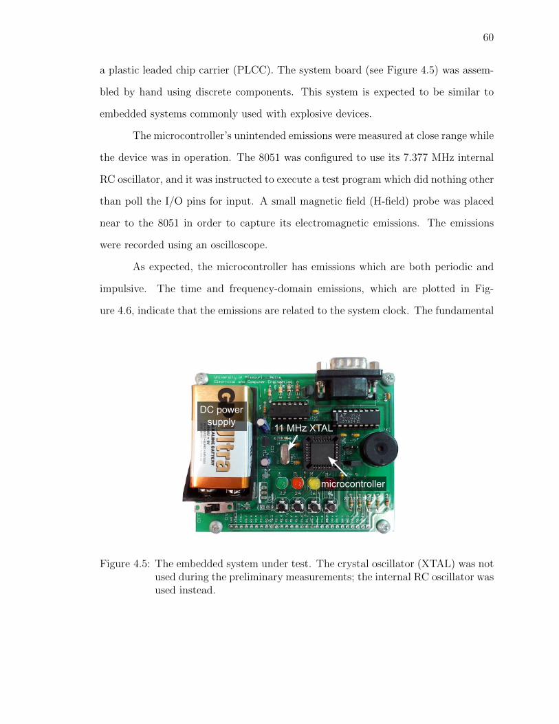
60
a plastic leaded chip carrier (PLCC). The system board (see Figure 4.5) was assem-
bled by hand using discrete components. This system is expected to be similar to
embedded systems commonly used with explosive devices.
The microcontroller’s unintended emissions were measured at close range while
the device was in operation. The 8051 was configured to use its 7.377 MHz internal
RC oscillator, and it was instructed to execute a test program which did nothing other
than poll the I/O pins for input. A small magnetic field (H-field) probe was placed
near to the 8051 in order to capture its electromagnetic emissions. The emissions
were recorded using an oscilloscope.
As expected, the microcontroller has emissions which are both periodic and
impulsive. The time and frequency-domain emissions, which are plotted in Fig-
ure 4.6, indicate that the emissions are related to the system clock. The fundamental
DC powersupply
microcontroller
11 MHz XTAL
Figure 4.5: The embedded system under test. The crystal oscillator (XTAL) was notused during the preliminary measurements; the internal RC oscillator wasused instead.

61
-100
-90
-80
-70
-60
-50
-40
-30
0 10 20 30 40 50 60 70 80
Pow
er(d
Bm
)
Frequency (MHz)
8051 Emissions: Frequency Domain
-30
-20
-10
0
10
20
0 2 4 6 8 10
Vol
tage
(mV
)
Time (periods)
8051 Emissions: Time Domain
Figure 4.6: Time and frequency-domain views of an 8051 microcontroller’s emissions.The clock frequency is estimated at 7.45 MHz. As anticipated, the emis-sions are a periodic impulse train. The pulses are in the negative directiondue to the alignment of the magnetic field probe. Although the 11 MHzcrystal oscillator was not used as the clock source, its harmonics are alsovisible in the plots above.

62
frequency of the emissions is approximately f0 = 7.45 MHz, which is within the spec-
ified tolerance of the RC oscillator’s frequency. The emissions are a harmonic signal,
and the first ten harmonics (f0 through f9) are present.
Epoch folding was used to obtain an estimate of the pulse shape. Although
the fast folding algorithm can detect the presence of microcontroller emissions, it is
less useful for estimating the period: the FFA’s output typically contains spurious
peaks in the vicinity of the true period. Since the goal is to make a very fine estimate
of the pulse shape, the period was estimated directly in the frequency domain, and
ordinary epoch folding was performed.
A multi-taper power spectral density (MTPSD) estimate was used to estimate
the period of the emissions. The MTPSD is an unbiased spectral density estimator,
and it has favorable resolution properties for making very fine frequency estimates
[69]. To limit the effects of long-term oscillator drift, the epoch fold contained only
769 clock periods of data. The emissions were then resampled, using a polyphase
filter bank, to exactly 26 samples per period.
The re-sampled emissions were folded across two separate periods (2T sam-
ples). The results of the fold, which are plotted with error bars in Figure 4.7, indicate
that the double-exponential AR model is a suitable approximation for clock emissions.
The variance of the folding bins is less than 7% of their magnitudes, which indicates
a good fit for the periodic signal model. The smaller peaks visible in the figure occur
at the falling edge of the clock, where another substantial current draw occurs due
to switching within the clock tree.
In Figure 4.8, the same data is folded across a single period. Linear prediction
is used to fit an AR(2) model to the data, and a single clock pulse is generated using
the estimated system filter. Both signals are aligned in time and normalized to a
peak value of one. The result of this process indicates that the AR(2) model is a

63
good fit in the vicinity of the main peak but loses accuracy elsewhere. This loss of
accuracy is due to a secondary peak, visible at approximately 0.6T .
This secondary peak, which is located half a period away from the main peak,
is caused by additional transistor switching. This additional switching takes place at
the falling edge of the clock, whereupon the clock tree resets itself for the next cycle.
The presence of this second peak will not affect the harmonic techniques, as the signal
is still periodic with a period of T . It may, however, reduce the effectiveness of linear
prediction with real CMOS emissions.
Although the emissions appear visually to be a good fit for the AR(2) model,
goodness-of-fit can be determined mathematically. If the signal is more complex
than the AR(2) model presumes, a higher autoregressive model order would provide
a better representation—i.e., a lower residual power. The optimum autoregressive
-25
-20
-15
-10
-5
0
5
10
0 0.5 1 1.5 2
Vol
tage
(mV
)
Time (periods)
Epoch Folding of 8051 Emissions
Figure 4.7: Epoch folding of 8051 electromagnetic emissions. The folding includestwo separate clock periods and is plotted with standard deviation errorbars.

64
model length can be found using information theory criterion, such as the Minimum
Description Length (MDL).
As formulated in [65], the MDL finds the minimum model order that is required
to represent a signal. It is evaluated as:
MDL(i) = L log var(e) + i logL, (4.17)
where i is the linear prediction order and L is the length of the input vector x from
(4.5). The epoch-folded emissions from the 8051 system were tested using linear
predictors of various orders, i = 1 through i = 10.
The results of this computation, given in Figure 4.9, indicate that the MDL
reaches a local minimum value at i = 2. The global minimum occurs at i = 4, but
-0.4
-0.2
0
0.2
0.4
0.6
0.8
1
0 0.2 0.4 0.6 0.8 1
Vol
tage
(∆)
Time (periods)
Exponential Fit of Folded 8051 Emissions
EmissionsAR(2) Fit
RMSE 0.20
Figure 4.8: The epoch-folded 8051 emissions and the ideal CMOS pulse determinedby linear prediction. The epoch folding is plotted with a solid line, and theideal CMOS pulse is plotted with a dashed line. The second peak near0.6T occurs at the falling edge of the clock, where another substantialcurrent draw takes place.

65
the difference is not particularly significant. The AR(2) model is a good choice to
represent this data set.
4.2.2. Simulated Environment. Since the autoregressive model fits real
CMOS emissions, detection algorithms can be tested through simulation. As in Sec-
tion 2.3, a simulated environment allows for controlled conditions, such as signal-to-
noise ratio, which are difficult to replicate consistently in a real system. The CMOS
clock pulses from Figure 4.1 were used as a test signal. The simulator assumes that
the channel corrupts the signal with additive white Gaussian noise.
White Gaussian noise is often a poor approximation of a radio channel. Chan-
nels may exhibit Rayleigh fading [78], frequency-selective fading [79], multipath prop-
agation [53], correlated noise, or numerous sources of man-made interference. The
goal of these tests is not to simulate radio propagation, however, but to determine
the relative performance of the detectors. Remedies for non-ideal noise conditions
exist, and some of them are detailed in Section 4.3.1.
-132
-130
-128
-126
-124
-122
0 2 4 6 8 10
MD
L
LPC ORder
Min. Description Length of Folded 8051 Emissions
Figure 4.9: The minimum description length (MDL) statistic. The MDL indicatesthat the AR(2) model is an appropriate approximation of 8051 clockemissions.

66
The simulator generates two test vectors,
x = c+ ν (4.18)
n = ν, (4.19)
where c is the CMOS emissions and ν is white, zero mean Gaussian noise (see Fig-
ure 4.2). The power of the noise is used to control the signal-to-noise ratio. The
vectors x and n are normalized to unit variance and used, individually, to test the
algorithms. The test statistics from the linear prediction (4.7), harmogram (4.8),
HPS (4.9), harmogrant (4.12), and FFA (4.16) algorithms are evaluated on each of
these inputs, producing output vectors of true positives and true negatives.
These test statistic vectors are used to generate Receiver Operating Char-
acteristic (ROC) curves for each algorithm. The ROC curves are generated as in
Section 2.3.2. A threshold detector, with the threshold set to various values, classi-
fies each of the above test statistics as a “detection” or a “non-detection,” and the
true positive rates and false positive rates are determined through simulation. In
cases where the test statistic contains multiple values—i.e., the harmogram power at
various frequencies—only the maximum value is considered.
The area under the ROC curve (AUC) is a commonly-accepted measure of
performance. The area represents the probability that a randomly-chosen true posi-
tive will have a larger-valued test statistic than a randomly-chosen true negative [80].
If the AUC is 1.0, the test perfectly separates true and false positives with a definite
decision threshold in between. If the AUC is 0.5, the test yields no useful information
as a detector.
The algorithms included in this study are not just detectors—they have in-
herent estimation capability as well. Both linear prediction and FFA can estimate
the pulse shape, and the FFA and pitch estimators can estimate the fundamental

67
frequency. For the purposes of this test, the estimation capability is not tested: only
the algorithms’ performance as a detector is considered.
In addition to white Gaussian noise, sinusoidal interference is considered. Si-
nusoidal signals can occur as communications signals (or as components thereof) or as
unintended emissions from radio receivers [12]. Since sinusoidal signals are strongly
concentrated in the frequency domain, they are among the most likely signals to cause
false positives with the pitch estimation algorithms. They may also disrupt the linear
prediction algorithms, as sinusoids also have an autoregressive representation [64].
Two test cases, with a single interfering sinusoid, were considered. The period
of the sinusoid was 0.75T , placing it halfway between two harmonics. The power of
the sinusoid was fixed at +10 dB above the noise power for the first test. For the
second test, it was defined to be +10 dB above the signal power instead, making it
a stronger signal. The interfering sinusoid is part of the noise vector n, making it
present regardless of whether or not the signal includes CMOS emissions. The results
of this simulation procedure are discussed in the following section.
4.2.3. Simulation Results. The simulation program was executed using
the CMOS emissions given in Figure 4.1 as input. SNRs between −15 dB and −35 dB
were tested, with one hundred independently-generated noise vectors ν tested at each
SNR level. Thirty thousand periods, with thirty samples per period, were simulated.
The pitch estimation algorithms and the FFA were limited to search the same
range of periods: from 0.7T to 3.33T . This limitation was put in place to reduce
the noise found in FFA folds of low-frequency data. The pitch detection algorithms
used a minimum of N = 4 harmonics and a maximum of N = 5 harmonics. After
simulating, the area under the curve (AUC) was calculated for each test case. The
results are summarized below.
For white Gaussian noise, plotted in Figure 4.10, the harmogrant outperformed
all other algorithms under each tested SNR. The results were similar to the traditional

68
harmogram, however, and the additional selectivity from the multiplication operation
provides only modest improvements. Linear prediction was less effective, and did not
perform substantially better than any of the pitch estimators. All the techniques
perfectly separated true and false positives above an SNR of -15 dB. In this test
case, the harmogrant offers a 4 dB increase in noise performance over the fast folding
algorithm.
The strong and weak sinusoidal results are plotted in Figure 4.11. The weak
sinusoidal stimulation had only a minimal effect on the algorithms. Even the har-
mogram, which has no inherent resistance to pure tones, was able to suppress the
unwanted signal. The strong sinusoid, whose results are plotted in Figure 4.11, causes
problems, however.
The unmodified harmogram selected, without fail, the strong interfering sinu-
soid as the most significant (i.e., strongest) signal of interest. Due to normalization,
0.5
0.55
0.6
0.65
0.7
0.75
0.8
0.85
0.9
0.95
1
-35 -30 -25 -20 -15
Are
a
SNR (dB)
ROC Area of Detection Algorithms
LPH-gram
HPSH-grant
FFAHPS
H-grant
Figure 4.10: Simulation results for CMOS signal in white noise. The harmogrant(“H-grant”) offers superior performance in all test cases.

69
0.5
0.55
0.6
0.65
0.7
0.75
0.8
0.85
0.9
0.95
1
-35 -30 -25 -20 -15
Are
a
SNR (dB)
ROC Area of Detection Algorithms
LPH-gram
HPSH-grant
FFA
H-grant
HPS
0.5
0.55
0.6
0.65
0.7
0.75
0.8
0.85
0.9
0.95
1
-35 -30 -25 -20 -15
Are
a
SNR (dB)
ROC Area of Detection Algorithms
LPH-gram
HPSH-grant
FFA
FFA
HPS
Figure 4.11: Simulation results for the weak sinusoid and strong sinusoid. The weaksinusoid (top) had minimal impact on the results, while the strong si-nusoid (bottom) substantially reduced the noise performance of mostalgorithms. The Fast Folding Algorithm is essentially immune to inter-fering sinusoids.

70
the periodogram-estimated power of the interfering sinusoid was slightly lower in the
“signal + noise” case than it was in the noise-only case. This reversed the behavior
of the detector statistics, resulting in AUCs that were below 0.5. The harmogrant’s
performance was also degraded by the interference—though only slightly.
The linear prediction algorithm performed well in the strong sinusoidal in-
terference case—slightly better than it did for pure additive noise. Although the
sinusoidal signal is autoregressive, it has poles near the unit circle, and the pulse
signal results in much lower-energy residuals. Since linear prediction minimizes the
residuals, it converged preferentially to the CMOS pulses.
The FFA and HPS were, predictably, unaffected by sinusoidal interference of
any variety. The FFA’s detector is highly specific to impulses, and HPS imposes a
large penalty for missing harmonics, giving them almost complete immunity to these
narrowband interferers.
4.3. DISCUSSION
The pitch estimation results clearly demonstrate the trade-off between sensi-
tivity and selectivity. The harmonic product spectrum is too selective to have good
noise performance. Due to the low-pass fall-off of the CMOS clock pulses, noise tends
to make the higher-order harmonics undetectable, rendering HPS inoperative. The
harmogram offers better noise performance, but it is quite vulnerable to single-tone
sinusoids. The harmogrant, a combination of the two algorithms, performs better in
all of above test cases.
The time-domain algorithms—linear prediction and epoch folding—have poor
noise performance. Problems with the detector statistic limited the performance of
the FFA. Despite normalizing by the estimated noise in (4.16), the statistic exhibits
frequency-dependent behavior. Epoch folds of white noise have a much higher power

71
level near DC than they do in the higher frequencies. Further study may yield
a more robust noise estimator. Although the time-domain algorithms have poorer
noise-performance, they may be more effective at discarding spurious, high-power
signals in the high-SNR regime.
Although these results are promising, the simulated environment cannot accu-
rately model all of the behaviors of a CMOS device. Devices such as microcontrollers
may execute a different instruction each clock cycle, causing the magnitude—or per-
haps even the duration—of the current pulses to vary. The impact of antennas, and
the potential availability of near and far-field radiation, is also an important con-
sideration. These behaviors are best tested by measuring real CMOS devices in an
actual RF propagation environment.
A number of issues remain before these algorithms can be implemented in a
practical digital device detector, however. Two of these issues—noise estimation and
clock jitter—are addressed in the following sections.
4.3.1. Constant False Alarm Rate. An optimum Neyman-Pearson detec-
tor uses a threshold test to determine if a signal of interest is present. The value of
the threshold depends on the desired probability of false alarm, which is set by the
user. Correctly setting this threshold requires knowledge of the probability density
function (pdf) of the noise [81], but this pdf is rarely known in practice. In order to
have a fixed probability of false alarm, it is necessary to set the threshold from the
data itself.
This family of techniques is known as Constant False Alarm Rate (CFAR). In
a CFAR algorithm, the noise level is first estimated from the data. Bins which exceed
a certain threshold, compared to the noise level, will trigger a detection. Sometimes
this threshold is set assuming that the noise has a particular distribution [82,83], but
other approaches simply use a constant gain above the noise level. CFAR can be
applied to, and is frequently applied to, power spectral density estimators.

72
In periodograms, CFAR can estimate the noise level for each bin individu-
ally. This makes the periodogram more robust against frequency-selective fading.
Such fading can occur as the result of, for example, non-flat frequency response
in the receiver or multipath propagation. While equalization can remove most of
these channel effects, most equalizers depend on knowing the transmitted signal very
precisely—which is difficult in this application [84].
CFAR processors operate on the assumption that any frequency-selective ef-
fects are gradual—i.e., the channel’s gain varies slowly with respect to frequency.
This enables the detector to assume that bins which are nearby in frequency have
similar noise powers. For each bin, the noise level is estimated using the surrounding
bins. If the bin under test contains a signal, that signal may also leak or spread into
surrounding bins. Hence, the closest bins are excluded from the noise estimate. The
process is illustrated in Figure 4.12.
A number of different noise estimation techniques exist. Cell-averaging CFAR
(CA-CFAR) estimates noise using the mean average, while order-statistic CFAR (OS-
CFAR) uses an order statistic. Each method has its own set of advantages and
drawbacks, but OS-CFAR has been shown to outperform CA-CFAR in most cases
[85]. Regardless of the technique in use, a CFAR processor is indispensable for a
practical CMOS clock detector.
4.3.2. Jitter. Microcontroller oscillators can exhibit considerable drift, and
any period estimate may not be valid for long. Systems which do not have particularly
demanding real-time constraints can use low-cost RC oscillators, and these oscillators
may have substantial long and short-term drift. Even crystal oscillators, which offer
higher precision, are not immune to environmental conditions [86].
Some oscillators deliberately add jitter in order to reduce their apparent unin-
tended emissions. These oscillators, which are known as spread spectrum clock gener-
ators (SSCGs), are of particular interest since they add jitter deterministically—and

73
are thus simpler to model than random drift. They are also of interest because they
may be more difficult to detect than standard oscillators—with pitch estimators in
particular. It is worth noting that an SSCG does not actually reduce the radiated
power—it merely spreads the radiated power over a wider range of frequencies.
SSCGs add jitter by making the oscillator’s target frequency a function of some
other periodic function. Each period, the time until the next clock pulse is selected
using the output of this spreading function. The spreading function is typically
symmetric about the oscillator’s “true” period, making the oscillator an accurate
timekeeper, on average. Triangle waves are popular spreading functions and are used
in practical SSCG devices [87,88].
In order to simulate the effect of a jittery oscillator, a spread spectrum clock
generator was used in the simulation. The simulated SSCG used a triangle-wave
Cell under test
Guard bins
Noise estimation bins
Frequency
Pow
er
CFAR Processing
Figure 4.12: The CFAR algorithm estimates the noise level for each bin using thesurrounding bins. The bins closest to the bin under test are ignored(guard bins). This process is repeated for each and every periodogrambin. The bins used for estimation are sometimes referred to as trainingbins.

74
spreading function that was 263 clock periods long and resulted in a maximum de-
viation of ±1% of the oscillator’s true period. These values were taken from a real
SSCG documented in [87].
The simulation results, which are plotted in Figure 4.13, show the fast folding
algorithm is particularly sensitive to jitter. The sub-sample folding accuracy of FFA
is more harmful than helpful in this case, as the peaks from the clock pulses are spread
into many different bins. The pitch estimators, which use only 2049 bins to represent
the entire signal, are much less sensitive to jitter. A decimation process may make
the FFA more resistant to jitter, but the pitch estimators offer better performance
at lower computational complexity.
In future work, cyclostationarity analysis may yield a more sensitive detector
for SSCGs. Unlike a stationary process, which has time-invariant statistical prop-
erties, a cyclostationary process has statistical properties which vary cyclically (i.e.,
0.5
0.55
0.6
0.65
0.7
0.75
0.8
0.85
0.9
0.95
1
-35 -30 -25 -20 -15
Are
a
SNR (dB)
ROC Area of Detection Algorithms
LPH-gram
HPSH-grant
FFA
H-grant
FFA
Figure 4.13: Simulation results for a jittery CMOS signal. The Fast Folding Algo-rithm is particularly sensitive to jitter.

75
periodically) in time [89]. In this case, the power spectrum of SSCGs varies cyclically
with respect to the spreading function. Cyclostationarity analysis has been proven
to be effective at detecting chirp radar [90], and it may be useful for detecting these
triangle wave-spread pulse trains as well.
4.4. CONCLUSION
Simulations indicate that pitch estimation algorithms offer the best noise per-
formance for detecting digital devices. These algorithms operate in the frequency
domain using periodograms as input, which makes them simple to implement on any
real-time device which has an FFT library. Periodograms have behaviors and trade-
offs, such as time/frequency resolution and windowing, which are well-understood
[23, 47, 91]. The harmogram, harmogrant, and the harmonic product spectrum do
not substantially increase the computational complexity of the periodogram, which
is given in [68].
While all of the pitch estimation algorithms performed well, the harmogrant
provided the best sensitivity and selectivity for this application. The harmogrant,
which is a minor, heuristic modification to the harmogram, has proven to be robust
against sinusoidal interference, low SNR, and typical jitter. This pitch estimation
technique offers a 4 dB gain in noise performance over the fast folding algorithm.
These findings re-enforce the usefulness of the Welch periodogram, and its relatives,
for detecting periodic signals.
Although the pitch estimation methods offer the highest performance, the
time-domain techniques are also useful. With sufficient signal-to-noise ratio, linear
prediction and the fast-folding algorithm also function “perfectly” with a ROC area
of 1.0. The fast folding algorithm is the most selective technique available: it only

76
detects impulse train signals. This selectivity may prove essential in real-world sce-
narios, where unexpected interference signals are present. Additional refinements
may make the FFA more robust against noise and jitter.
Linear prediction offers no particular advantage over the other techniques,
but the autoregressive model it is based on is useful for modeling clock emissions.
Comparisons with real data, gathered from an 8051 microcontroller, indicate that a
second-order autoregressive model is a reasonable approximation of clock emissions.
The model holds even when the emissions are received via a loop probe, which uses
inductive coupling.
These findings, while preliminary, demonstrate the feasibility of building a
digital device detector. The harmogrant and fast folding algorithms have promising
simulated results and, in future work, could be tested in a real-time detector under
real propagation conditions. With additional measurements and testing, the methods
proposed herein could enable the rapid discovery of digital devices.

77
APPENDIX
Measuring stimulated emissions requires two vital radio frequency (RF) com-
ponents: a transmitter and a receiver. In prior research conducted in Seguin [92],
these measurements were conducted using traditional lab equipment: signal genera-
tors, spectrum analyzers, and oscilloscopes. This approach has a number of important
drawbacks, however. Most signal generators are strictly-analog systems which can
only perform analog modulations, such as AM and FM. This necessitates the use of
additional hardware, such as waveform generators, to produce the desired stimulation
signal.
The receiver side, depending on the exact configuration, was similarly compli-
cated. A variety of analog mixers and filters were used to lower the frequency of the
unintended emissions, allowing them to be sampled at lower rates. Digital sampling
was performed using oscilloscopes, which posed their own set of difficulties. Oscil-
loscopes have a finite memory space for digital samples, and the oscilloscopes used
in [92] could only capture several consecutive milliseconds of data before exhausting
this space.
Once the samples were obtained, they were transferred to a personal computer
(PC) for further processing. This step required the use of slow, low-throughput IEEE-
488 (GPIB) interfaces. As a result, the stimulated emissions system developed in [92]
could only sample intermittently, and the data transfer itself introduced over one
second of latency. The complete measurement setup consisted of numerous pieces of
bulky, fragile equipment, and it was not particularly portable. This system was built
as part of the preliminary investigation of the stimulated emissions approach, which
was successful, however more convenient solutions exist.

78
Software-defined radio (SDR) platforms replace purpose-built analog commu-
nications circuitry with high-speed digital signal processing (DSP). As its name im-
plies, most of the radio signal processing takes place in software: typically on a
standard PC. An SDR digitizes radio signals in much the same way that a sound
card digitizes audio, except that the process takes place at a much higher speed. The
components of an SDR system are illustrated in Figure 5.1
The hardware component of an SDR system, often referred to as the “front-
end,” is designed to be minimalist and flexible. An analog radio receiver—either
superheterodyne or direct-conversion—is used to select the desired frequency and
bandwidth. The signal is then sampled using high-speed analog to digital converters
(ADCs). A comprehensive overview of the digitization process can be found in [93].
Some ADCs operate fast enough that the analog front-end can be omitted entirely.
The limiting factor in an SDR system is, typically, the interconnect between
the front-end and the host computer. This interconnect, such as Universal Serial Bus
(USB) or PCI Express, has limited throughput—i.e., USB 2.0 has a maximum transfer
Tuning Down-conversion
Analog toDigital
HostInterface
AnalogHardware
Real-timeDigital System
HostComputer
Figure 5.1: A software-defined radio system. The hardware components, includingthe real-time digital system, are designed to be as minimalist as possible.This grants the host computer more flexible access to the radio signal andspectrum.

79
rate of about 32 MiB/s. In order to meet real-time deadlines, it is necessary to limit
the data rate to that of the interconnect. This is accomplished by discarding the
unnecessary portions of the radio signal: a process known as digital down-conversion.
Digital down-conversion is the digital equivalent of analog frequency trans-
lation. The signal is shifted in frequency until the band of interest is centered at
baseband. (Quadrature sampling is used to preserve the magnitude and phase of
the signal.) The signal is then band-limited, using digital filters, to the frequency
range of interest. Once it has been filtered, the sampling rate can be reduced without
distorting the signal. The reduction in sampling rate greatly decreases the amount
of data that must be transferred and processed.
Once the data is transferred to the host computer, application-specific signal
processing is performed. Typically, these tasks include demodulation and, for data
signals, framing. In stimulated emissions, the goal is to search the down-converted
radio signal for the presence of some known stimulation signal. The algorithms to do
so can be written in ordinary, general-purpose computer languages such as C++ and
Python.
The principal advantage of software-defined radio is flexibility. The same SDR
platform can perform many different tasks, often simultaneously. Changing the DSP
algorithm is as simple as altering the software. Computer systems have access to
advanced user interfaces, built-in debuggers, and nearly-unlimited storage, making
them an attractive alternative to dedicated hardware. It is no surprise that SDRs
are popular with research and other non-recurring engineering tasks [94].
The papers in Section 2 and Section 3 developed two major software-defined
radio projects, both for research and for demonstration purposes. These projects,
which are detailed in the next two sections, are intended to validate the effectiveness
of stimulated emissions. They also, by extension, demonstrate the usefulness of SDR
to research and academia.

80
MATCHED FILTER DETECTOR
Many different SDR platforms are available, ranging from hobbyist kits
($20 U.S. Dollars) to purpose-built computer systems for maximum sensitivity and
throughput ($7000 U.S. Dollars or more). The matched filter detector used in
Section 2 was built using the Ettus Research Universal Software Radio Peripheral
(USRP), which was selected due to its proven performance and wide range of avail-
able transceiver modules. The USRP’s companion software, GNU Radio, is designed
to support real-time designs. The DSP operations (i.e., functions) are described us-
ing the Python scripting language. When the system is started, these operations are
executed continuously on the incoming data from the SDR [21].
The matched filter detector is designed to detect superheterodyne receivers
using the method outlined earlier in this chapter. As per Figure 2.7, the system
detects radio receivers by transmitting a 5kHz linear FM chirp and searching for the
chirp on another, defined frequency using a matched filter. When the program is
started, it generates a baseband, complex-sampled chirp of a user-specified length.
The chirp’s matched filter, which is a finite impulse response (FIR) digital filter, is
then derived and stored. This detector is implemented entirely using the USRP’s
companion software, GNU Radio.
The program then instructs the USRP to transmit this chirp repetitively and
sample the radio spectrum at the up-mixing emissions frequency. The received signal
is then filtered through the matched filter. If a radio receiver is present, the matched
filter will output an impulse-like spike every chirp period. A threshold detector is
used to decide if a radio receiver has been detected: The power output of the matched
filter is compared with a fixed, user-specified threshold, and a detection is declared
if the power exceeds the threshold [81].

81
The matched filter detector includes a simple GUI, shown in Figure 5.2, for
setting and viewing the detector’s threshold. A visual and audible alarm are activated
if a radio receiver is detected. The detector operates in real-time, updating its display
continuously as new data is received. The complete hardware setup, as shown in
Figure 5.3, fits neatly on a tabletop and is easy to transport.
This real-time implementation offers substantial advantages over the sample-
then-process design used for initial investigations in Seguin. Long-duration chirps,
Figure 5.2: The simple GUI for the matched filter detector. The image of the radioreceiver indicates that a device has been detected.
Amp
USRP
Laptop
RX Ant
TX Ant
Figure 5.3: The assembled USRP test setup fits neatly on a table top. It can bedisassembled and stored in a small box for transport.

82
which exceed one second in length, can be used without difficulty. Troubleshooting
physical problems, such as antenna leakage or cross-coupling, is vastly simplified when
the detector statistic updates quickly. The matched filter detector program offers an
easy-to-understand demonstration of the stimulated emissions technique. Although
the hardware used in [92] was commonly available, and more than adequate for a
preliminary study, the SDR platform resulted in a much simpler, easy-to-use system.
SOFTWARE-DEFINED RADAR
Locating superheterodyne receivers using the time-of-arrival method, as dis-
cussed in Section 3, requires high-precision timing. The SDR must be capable of
accurately measuring the time difference between the transmission of the stimula-
tion and the reception of the emissions. For speed-of-light signals, a timing error of
just ten nanoseconds translates into one meter of range error. This is a strict real-
time synchronization demand which cannot be met using general-purpose computer
programs. Designing an SDR to meet these demands is a challenging task.
From [12], it is known that superheterodyne receivers are highly responsive
to linear FM chirps. Using a technique known as frequency-modulated continuous
wave (FMCW) radar, it is possible to use similar chirp signals for ranging in addition
to detection. In continuous-wave radar, the power of the transmitted stimulation is
kept constant. Constant-power signals perform well with systems that use solid-state,
low-noise amplifiers—as superheterodyne receivers typically do [40]. FMCW has a
computationally-efficient implementation which makes it ideal for SDR.
In [95], it is demonstrated that delaying a linear FM chirp in time is equivalent
to shifting it in frequency. In radar systems, the time-delayed return signal—in
this case, the emissions from the target device—appears to be slightly shifted in
frequency. This frequency shift, as shown in Figure 5.4, can be estimated by finding

83
the instantaneous difference in frequency between the transmitted stimulation and
the received emissions. This difference can be found using mixers.
In the mixer implementation, the received emissions are mixed with a time-
reversed version of the transmitted stimulation. The result is a low-frequency “beat”
signal which contains the range information. Traditional estimators of frequency,
such as the Fast Fourier Transform (FFT), can be used to estimate the beat signal’s
frequency—and thus the range. This design is ideal for use on software-defined radio
platforms: The mixing is a mathematically simple—but time-sensitive—operation,
whereas the frequency estimation can benefit from the processing power of a general-
purpose computer.
To fulfill the real-time requirement, an FMCW front-end was added to the
USRP. The front-end generates the linear FM chirps and performs a simultaneous
de-chirp of the received emissions. To guarantee a fixed delay, these operations were
Chirp
Time/Freq. Duality
Time
Fre
quen
cy
Freq. Shift
dt
df
T
F=
df
dt F
T
Figure 5.4: Delaying a linear FM chirp in time by some amount dt is equivalent toshifting it in frequency by some amount df . This relationship is easy tovisualize from the proportional triangles given above. By estimating thefrequency difference df , it is possible to estimate the time delay dt.

84
implemented in the USRP’s field-programmable gate array (FPGA). The FPGA typi-
cally performs the high-speed digital down-conversion (see Figure 5.1), but it supports
loading user-customized instruction sets as well. This customization is made possi-
ble, in part, by the USRP’s open-source design. After de-chirping, the resulting beat
signal is down-converted and sent to the host computer.
The host computer then estimates the frequency of the beat signal. A two-
dimensional FFT, as per [43], simultaneously estimates both the range to and Doppler
shift of a target. The entire software-defined radar system is depicted in Figure 5.5.
Since it was designed for stimulated emissions, this radar system has one additional
feature: it can transmit and receive on different, arbitrary frequencies. This enables
the radar system to receive and detect up-mixing emissions from superheterodyne
receivers.
This prototype system demonstrates the extensibility of software-defined ra-
dio platforms. Owing to their advanced computer software and re-programmable
circuitry (i.e., FPGAs), such platforms can be modified to function far beyond their
Transmitter
Front-end
RxAnt.
TxAnt.
Receiver
Front-end
Time
Fre
q
TargetDevice
?
Time
Fre
q
FFT2
Range-Doppler
Processor
Down-conversion
ChirpGenerator
De-chirp
AnalogHardware
Real-timeDigital System
HostComputer
USBPost-
processing
Figure 5.5: Block diagram of the software-defined radar. A chirp generator, anda synchronized de-chirp function, were added to the USRP’s FPGAfirmware. The range-doppler processing is carried out on the host PC.Adapted from [13], c© 2013, IEEE. Used with permission.

85
original design specifications. The system described above was successfully tested
in [13], where it accurately measured the range to various superheterodyne receivers.
While isolation problems between the transmitter and receiver substantially reduced
the system’s performance, these problems occurred in the analog front-end and are
not specific to SDR.
As this research demonstrates, software-defined radio products greatly increase
the accessibility of the radio spectrum to academic researchers. These devices can
facilitate the development of novel communications and signal processing techniques,
and it is worthwhile to consider them whenever rapid prototyping is desired.

86
BIBLIOGRAPHY
[1] Y. Fu, G. Burbui, and T. Hubing, “An improved model for representing cur-rent waveforms in CMOS circuits,” Clemson University Vehicular ElectronicsLaboratory, Tech. Rep. CVEL-06-001, Oct 2006.
[2] 110th United States Congress, “Department of homeland security appropriationsbill, 2009,” GPO, Washington D.C., Tech. Rep., June 2008.
[3] A. J. Davidson, S. Chellappa, Raja, D. M. Dattelbaum, and C.-S. Yoo, “Pres-sure induced isostructural metastable phase transition of ammonium nitrate,”J. Phys. Chem. A, vol. 115, no. 42, pp. 11 889–11 896, 2011.
[4] J. Dai, B. Clough, I.-C. Ho, X. Lu, J. Liu, and X.-C. Zhang, “Recent progresses interahertz wave air photonics,” IEEE Trans. Terahertz Science and Tech., vol. 1,no. 1, pp. 274–281, 2011.
[5] L. Pacheco-Londono, W. Ortiz-Rivera, O. Primera-Pedrozo, and S. Hernandez-Rivera, “Vibrational spectroscopy standoff detection of explosives,” Analyticaland Bioanalytical Chemistry, vol. 395, pp. 323–335, 2009.
[6] M. Nambayah and T. I. Quickenden, “A quantitative assessment of chemicaltechniques for detecting traces of explosives at counter-terrorist portals,” Ta-lanta, vol. 63, no. 2, pp. 461 – 467, 2004.
[7] C. Wilson, “Improvised explosive devices (IEDs) in Iraq: Effects and counter-measures,” Library of Congress, Washington D.C., Congressional Research Ser-vice Report RS22330, Feb 2006.
[8] C. Griffith, “Unmanned aerial vehicle-mounted high sensitivity rf receiver to de-tect improvised explosive devices,” Master’s thesis, Naval Postgraduate School,2007.
[9] H. Sekiguchi and S. Seto, “Proposal of an information signal measurementmethod in display image contained in electromagnetic noise emanated from apersonal computer,” in Proc. IEEE Instrum. and Measure. Tech. Conf., 2008,pp. 1859–1863.
[10] “Title 47–Telecommunication §15,” Code of Federal Regulations, FCC, Oct 1998.
[11] I. Smith and M. Coderre, “The continuing war against ieds,” WSTIAC Quar-terly, vol. 8, no. 2, pp. 3–6, April 2008.

87
[12] C. Stagner, A. Conrad, C. Osterwise, D. Beetner, and S. Grant, “A practicalsuperheterodyne-receiver detector using stimulated emissions,” IEEE Trans.Instrum. Meas., vol. 60, no. 4, pp. 1461–1468, 2011. [Online]. Available:http://dx.doi.org/10.1109/TIM.2010.2101330.
[13] C. Stagner, M. Halligan, C. Osterwise, D. Beetner, and S. Grant, “Locatingnoncooperative radio receivers using wideband stimulated emissions,” IEEETrans. Instrum. Measure., vol. 62, no. 3, pp. 667–674, 2013. [Online]. Available:http://dx.doi.org/10.1109/TIM.2012.2219141.
[14] D. Beetner, S. Seguin, and H. Hubing, “Electromagnetic emissions stimulationand detection system,” U.S. Patent 7 464 005, 2008.
[15] B. Wild and K. Ramchandran, “Detecting primary receivers for cognitive radioapplications,” in Proc. 1st IEEE Int’l Symp. DySPAN, Nov. 2005, pp. 124–130.
[16] A. Shaik, H. Weng, X. Dong, T. Hubing, and D. Beetner, “Matched filter detec-tion and identification of electronic circuits based on their unintentional radiatedemissions,” in Proc. IEEE ISEMC, vol. 3, 2006.
[17] S. Seguin, “Detection of low cost radio frequency receivers based on theirunintended electromagnetic emissions and an active stimulation,” Ph.D.dissertation, Missouri S&T, 2009. [Online]. Available: http://scholarsmine.mst.edu/thesis/pdf/Seguin 09007dcc80708216.pdf.
[18] R. Bracewell, The Fourier Transform and Its Applications, 3rd ed. McGraw-Hill, 1999, p. 108.
[19] T. Nguyen, S. Koppen, J. Ely, R. Williams, L. Smith, M. Salud, L. Martin, andV. Hampton, “Portable wireless LAN device and two-way radio threat assess-ment for aircraft VHF communication radio band,” NASA Langley Res. Center,NASA/TM-2004-213010, 2004.
[20] R. Oki and T. Ebisawa, “Double Superheterodyne Receiver,” U.S. Patent4 395 777, 1983.
[21] P. Ferrari, A. Flammini, and E. Sisinni, “Introducing the Wireless Ultra SmartSensor,” in Proc. IEEE I2MTC, 2009, pp. 1304–1308.
[22] “Title 47–Telecommunication §95a,” Code of Federal Regulations, FCC, Oct1998.
[23] H. So, Y. Chan, Q. Ma, and P. Ching, “Comparison of various periodograms forsinusoid detection and frequency estimation,” IEEE Trans. AES, vol. 35, no. 3,pp. 945–952, 2002.
[24] G. Turin, “An introduction to matched filters,” IRE Trans. Inf. Theory, vol. 6,no. 3, pp. 311–329, June 1960.
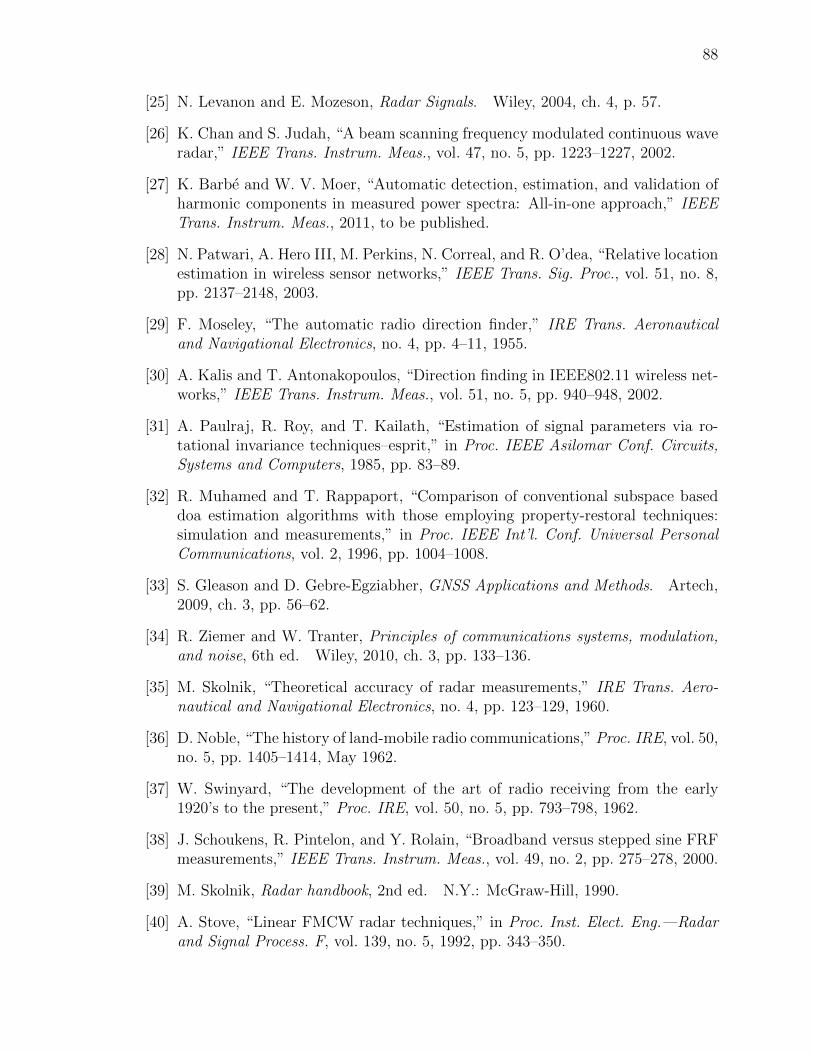
88
[25] N. Levanon and E. Mozeson, Radar Signals. Wiley, 2004, ch. 4, p. 57.
[26] K. Chan and S. Judah, “A beam scanning frequency modulated continuous waveradar,” IEEE Trans. Instrum. Meas., vol. 47, no. 5, pp. 1223–1227, 2002.
[27] K. Barbe and W. V. Moer, “Automatic detection, estimation, and validation ofharmonic components in measured power spectra: All-in-one approach,” IEEETrans. Instrum. Meas., 2011, to be published.
[28] N. Patwari, A. Hero III, M. Perkins, N. Correal, and R. O’dea, “Relative locationestimation in wireless sensor networks,” IEEE Trans. Sig. Proc., vol. 51, no. 8,pp. 2137–2148, 2003.
[29] F. Moseley, “The automatic radio direction finder,” IRE Trans. Aeronauticaland Navigational Electronics, no. 4, pp. 4–11, 1955.
[30] A. Kalis and T. Antonakopoulos, “Direction finding in IEEE802.11 wireless net-works,” IEEE Trans. Instrum. Meas., vol. 51, no. 5, pp. 940–948, 2002.
[31] A. Paulraj, R. Roy, and T. Kailath, “Estimation of signal parameters via ro-tational invariance techniques–esprit,” in Proc. IEEE Asilomar Conf. Circuits,Systems and Computers, 1985, pp. 83–89.
[32] R. Muhamed and T. Rappaport, “Comparison of conventional subspace baseddoa estimation algorithms with those employing property-restoral techniques:simulation and measurements,” in Proc. IEEE Int’l. Conf. Universal PersonalCommunications, vol. 2, 1996, pp. 1004–1008.
[33] S. Gleason and D. Gebre-Egziabher, GNSS Applications and Methods. Artech,2009, ch. 3, pp. 56–62.
[34] R. Ziemer and W. Tranter, Principles of communications systems, modulation,and noise, 6th ed. Wiley, 2010, ch. 3, pp. 133–136.
[35] M. Skolnik, “Theoretical accuracy of radar measurements,” IRE Trans. Aero-nautical and Navigational Electronics, no. 4, pp. 123–129, 1960.
[36] D. Noble, “The history of land-mobile radio communications,” Proc. IRE, vol. 50,no. 5, pp. 1405–1414, May 1962.
[37] W. Swinyard, “The development of the art of radio receiving from the early1920’s to the present,” Proc. IRE, vol. 50, no. 5, pp. 793–798, 1962.
[38] J. Schoukens, R. Pintelon, and Y. Rolain, “Broadband versus stepped sine FRFmeasurements,” IEEE Trans. Instrum. Meas., vol. 49, no. 2, pp. 275–278, 2000.
[39] M. Skolnik, Radar handbook, 2nd ed. N.Y.: McGraw-Hill, 1990.
[40] A. Stove, “Linear FMCW radar techniques,” in Proc. Inst. Elect. Eng.—Radarand Signal Process. F, vol. 139, no. 5, 1992, pp. 343–350.
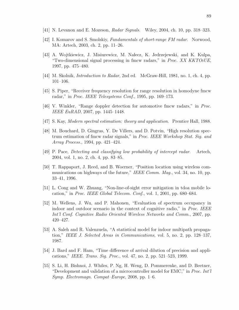
89
[41] N. Levanon and E. Mozeson, Radar Signals. Wiley, 2004, ch. 10, pp. 318–323.
[42] I. Komarov and S. Smolskiy, Fundamentals of short-range FM radar. Norwood,MA: Artech, 2003, ch. 2, pp. 11–26.
[43] A. Wojtkiewicz, J. Misiurewicz, M. Na lecz, K. Jedrzejewski, and K. Kulpa,“Two-dimensional signal processing in fmcw radars,” in Proc. XX KKTOiUE,1997, pp. 475–480.
[44] M. Skolnik, Introduction to Radar, 2nd ed. McGraw-Hill, 1981, no. 1, ch. 4, pp.101–106.
[45] S. Piper, “Receiver frequency resolution for range resolution in homodyne fmcwradar,” in Proc. IEEE Telesystems Conf., 1995, pp. 169–173.
[46] V. Winkler, “Range doppler detection for automotive fmcw radars,” in Proc.IEEE EuRAD, 2007, pp. 1445–1448.
[47] S. Kay, Modern spectral estimation: theory and application. Prentice Hall, 1988.
[48] M. Bouchard, D. Gingras, Y. De Villers, and D. Potvin, “High resolution spec-trum estimation of fmcw radar signals,” in Proc. IEEE Workshop Stat. Sig. andArray Process., 1994, pp. 421–424.
[49] P. Pace, Detecting and classifying low probability of intercept radar. Artech,2004, vol. 1, no. 2, ch. 4, pp. 83–85.
[50] T. Rappaport, J. Reed, and B. Woerner, “Position location using wireless com-munications on highways of the future,” IEEE Comm. Mag., vol. 34, no. 10, pp.33–41, 1996.
[51] L. Cong and W. Zhuang, “Non-line-of-sight error mitigation in tdoa mobile lo-cation,” in Proc. IEEE Global Telecom. Conf., vol. 1, 2001, pp. 680–684.
[52] M. Wellens, J. Wu, and P. Mahonen, “Evaluation of spectrum occupancy inindoor and outdoor scenario in the context of cognitive radio,” in Proc. IEEEInt’l Conf. Cognitive Radio Oriented Wireless Networks and Comm., 2007, pp.420–427.
[53] A. Saleh and R. Valenzuela, “A statistical model for indoor multipath propaga-tion,” IEEE J. Selected Areas in Communications, vol. 5, no. 2, pp. 128–137,1987.
[54] J. Bard and F. Ham, “Time difference of arrival dilution of precision and appli-cations,” IEEE. Trans. Sig. Proc., vol. 47, no. 2, pp. 521–523, 1999.
[55] S. Li, H. Bishnoi, J. Whiles, P. Ng, H. Weng, D. Pommerenke, and D. Beetner,“Development and validation of a microcontroller model for EMC,” in Proc. Int’lSymp. Electromagn. Compat–Europe, 2008, pp. 1–6.

90
[56] S. Orfanidis, Optimum signal processing: An introduction, 2nd ed. N.Y.:McGraw-Hill, 1988, ch. 6, pp. 248–259.
[57] N. Ravirala, “Device signal detection methods and time frequency analysis,”Master’s thesis, University of Missouri–Rolla, 2007. [Online]. Available:http://scholarsmine.mst.edu/thesis/pdf/Ravirala 09007dcc803fea67.pdf.
[58] R. Zelinski, “A microphone array with adaptive post-filtering for noise reductionin reverberant rooms,” in IEEE Int’l. Conf. Acoustics, Speech, and Sig. Proc.,vol. 5, apr 1988, pp. 2578 – 2581.
[59] I. Flintoft, A. Marvin, M. Robinson, K. Fischer, and A. Rowell, “The re-emissionspectrum of digital hardware subjected to emi,” IEEE Trans. ElectromagneticCompatibility, vol. 45, no. 4, pp. 576–585, 2003.
[60] K. Hu, H. Weng, D. Beetner, D. Pommerenke, J. Drewniak, K. Lavery, andJ. Whiles, “Application of chip-level emc in automotive product design,” inElectromagnetic Compatibility, 2006. EMC 2006. 2006 IEEE International Sym-posium on, vol. 3, 2006, pp. 842–848.
[61] D. Panyasak, G. Sicard, and M. Renaudin, “A current shaping methodology forlowering EM disturbances in asynchronous circuits,” Microelectronics journal,vol. 35, no. 6, pp. 531–540, 2004.
[62] Y. Fu, G. Burbui, and T. Hubing, “An improved model for representing cur-rent waveforms in cmos circuits,” in Proc. IEEE Int’l. Symp. ElectromagneticCompatibility, 2007, pp. 289–292.
[63] M. Schroeder and B. Atal, “Code-excited linear prediction (celp): High-qualityspeech at very low bit rates,” in IEEE Int’l Conf. Acoustics, Speech, and Sig.Proc., vol. 10, 1985, pp. 937–940.
[64] D. Percival and A. Walden, Spectral analysis for physical applications. Cam-bridge University Press, 1993, ch. 9, pp. 391–455.
[65] M. H. Hansen and B. Yu, “Model selection and the principle of minimum de-scription length,” Journal of the American Statistical Association, vol. 96, no.454, pp. 746–774, 2001.
[66] A. N. Iyer, M. Gleiter, B. Y. Smolenski, and R. E. Yantorno, “Structural usablespeech measure using lpc residual,” in International Symposium on IntelligentSignal Processing and Communication Systems, vol. 2, no. 3, 2003, pp. 236–240.
[67] D. Percival and A. Walden, Spectral analysis for physical applications. Cam-bridge University Press, 1993, ch. 3, pp. 56–125.
[68] P. Welch, “The use of fast fourier transform for the estimation of power spectra:a method based on time averaging over short, modified periodograms,” IEEETrans. Audio and Electroacoustics, vol. 15, no. 2, pp. 70–73, 1967.

91
[69] D. Percival and A. Walden, Spectral analysis for physical applications. Cam-bridge University Press, 1993, ch. 7, pp. 331–377.
[70] A. De Cheveigne and H. Kawahara, “Yin, a fundamental frequency estimatorfor speech and music,” J. of Acoustical Society of America, vol. 111, p. 1917,2002.
[71] T. Shimamura and H. Kobayashi, “Weighted autocorrelation for pitch extractionof noisy speech,” IEEE Trans. Speech and Audio Processing, vol. 9, no. 7, pp.727–730, 2001.
[72] M. Hinich, “Detecting a hidden periodic signal when its period is unknown,”IEEE Trans. Acoustics, Speech and Sig. Proc., vol. 30, no. 5, pp. 747–750, 1982.
[73] M. Noll, “Pitch determination of human speech by the harmonic product spec-trum, the harmonic sum spectrum, and a maximum likelihood estimate,” inProc. Symposium on Computer Processing Communications, 1969, pp. 779–797.
[74] D. Staelin, “Fast folding algorithm for detection of periodic pulse trains,” Proc.IEEE, vol. 57, no. 4, pp. 724–725, 1969.
[75] V. Kondratiev, M. McLaughlin, D. Lorimer, M. Burgay, A. Possenti, R. Turolla,S. Popov, and S. Zane, “New limits on radio emission from x-ray dim isolatedneutron stars,” The Astrophysical Journal, vol. 702, no. 1, p. 692, 2009.
[76] S. Davies, “An improved test for periodicity,” Monthly Notices of the RoyalAstronomical Society, vol. 244, pp. 93–95, 1990.
[77] S. Larsson, “Parameter estimation in epoch folding analysis,” Astronomy andAstrophysics Supplement Series, vol. 117, no. 1, pp. 197–201, 1996.
[78] C. S. Patel, G. L. Stuber, and T. G. Pratt, “Comparative analysis of statisti-cal models for the simulation of rayleigh faded cellular channels,” IEEE Trans.Commun., vol. 53, no. 6, pp. 1017–1026, 2005.
[79] J. G. Proakis and D. G. Manolakis, Digital communications, 5th ed. McGraw-hill, 2008, ch. 13, pp. 869–884.
[80] M. H. Zweig and G. Campbell, “Receiver-operating characteristic (roc) plots:a fundamental evaluation tool in clinical medicine.” Clinical chemistry, vol. 39,no. 4, pp. 561–577, 1993.
[81] H. L. Van Trees, Detection, estimation, and modulation theory. Wiley, 2001,ch. 2, pp. 23–46.
[82] M. Xiangwei, G. Jian, and W. Xinzheng, “Order statistics for negative exponen-tial distribution and its applications,” in Proc. IEEE Int’l. Conf. Neural Net.and Sig. Proc., vol. 1, 2003, pp. 720–722.
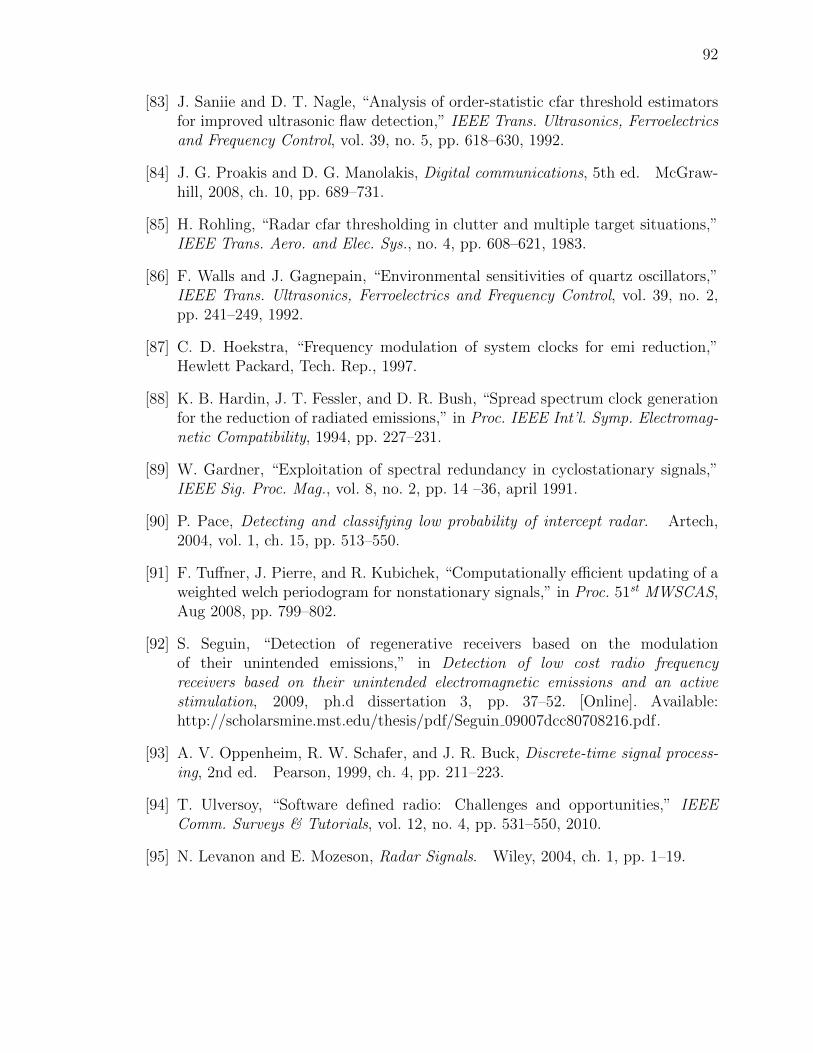
92
[83] J. Saniie and D. T. Nagle, “Analysis of order-statistic cfar threshold estimatorsfor improved ultrasonic flaw detection,” IEEE Trans. Ultrasonics, Ferroelectricsand Frequency Control, vol. 39, no. 5, pp. 618–630, 1992.
[84] J. G. Proakis and D. G. Manolakis, Digital communications, 5th ed. McGraw-hill, 2008, ch. 10, pp. 689–731.
[85] H. Rohling, “Radar cfar thresholding in clutter and multiple target situations,”IEEE Trans. Aero. and Elec. Sys., no. 4, pp. 608–621, 1983.
[86] F. Walls and J. Gagnepain, “Environmental sensitivities of quartz oscillators,”IEEE Trans. Ultrasonics, Ferroelectrics and Frequency Control, vol. 39, no. 2,pp. 241–249, 1992.
[87] C. D. Hoekstra, “Frequency modulation of system clocks for emi reduction,”Hewlett Packard, Tech. Rep., 1997.
[88] K. B. Hardin, J. T. Fessler, and D. R. Bush, “Spread spectrum clock generationfor the reduction of radiated emissions,” in Proc. IEEE Int’l. Symp. Electromag-netic Compatibility, 1994, pp. 227–231.
[89] W. Gardner, “Exploitation of spectral redundancy in cyclostationary signals,”IEEE Sig. Proc. Mag., vol. 8, no. 2, pp. 14 –36, april 1991.
[90] P. Pace, Detecting and classifying low probability of intercept radar. Artech,2004, vol. 1, ch. 15, pp. 513–550.
[91] F. Tuffner, J. Pierre, and R. Kubichek, “Computationally efficient updating of aweighted welch periodogram for nonstationary signals,” in Proc. 51st MWSCAS,Aug 2008, pp. 799–802.
[92] S. Seguin, “Detection of regenerative receivers based on the modulationof their unintended emissions,” in Detection of low cost radio frequencyreceivers based on their unintended electromagnetic emissions and an activestimulation, 2009, ph.d dissertation 3, pp. 37–52. [Online]. Available:http://scholarsmine.mst.edu/thesis/pdf/Seguin 09007dcc80708216.pdf.
[93] A. V. Oppenheim, R. W. Schafer, and J. R. Buck, Discrete-time signal process-ing, 2nd ed. Pearson, 1999, ch. 4, pp. 211–223.
[94] T. Ulversoy, “Software defined radio: Challenges and opportunities,” IEEEComm. Surveys & Tutorials, vol. 12, no. 4, pp. 531–550, 2010.
[95] N. Levanon and E. Mozeson, Radar Signals. Wiley, 2004, ch. 1, pp. 1–19.

93
VITA
Colin Blake Stagner, better known to his friends and colleagues as “Chibi,”
was born in mid-1986 in a small college town. At a young age, Colin taught himself
programming, graph theory, and networking protocols by writing automatic game-
playing scripts for bulletin board system games. Before graduating from high school,
he had written his first database-driven website, which saw active use for many years
thereafter.
As an undergraduate, Colin contributed to university research both directly,
through the Computer Science department, and indirectly as a circulation staff mem-
ber at the Curtis Laws Wilson library. He also served as an officer of the Society of
Women Engineers for three consecutive years. Colin was awarded a Bachelor of Sci-
ence degree in 2008 by the University of Missouri–Rolla, which is now known as the
Missouri University of Science and Technology (S&T). He graduated summa cum
laude with a degree in Computer Science.
Soon after graduation, Colin returned to his alma mater to begin work on his
doctorate degree. He changed majors after accepting a Graduate Research Assistant
position from Dr. Steve Grant in the Electrical Engineering department. There,
he studied digital signal processing—a discipline which melds computer and electric
systems with the physical world. His principal contribution to the field was a software-
defined radar system for locating radio receivers. As part of a class project, he also
developed a digital communications receiver for amateur radio, which he uses to
receive transmissions from the International Space Station. He became Dr. Colin
Stagner in December 2013 when he was awarded a Ph.D. from S&T.