Embed Size (px)
Citation preview

Detecting Abnormalities in
Aircraft Flight Data and Ranking
their Impact on the Flight
Edward Smart
Institute of Industrial Research
University of Portsmouth
A thesis submitted for the degree of
Doctor of Philosophy
20th April 2011
brought to you by COREView metadata, citation and similar papers at core.ac.uk
provided by OpenGrey Repository

Whilst registered as a candidate for the above degree, I have not
been registered for any other research award. The results and
conclusions embodied in this thesis are the work of the named
candidate and have not been submitted for any other academic
award.

I would like to dedicate this thesis to my family, Martin, Ruth,
Bryony, Adrian and also to my girlfriend, Kelly.

Acknowledgements
Completing this PhD has given me immense satisfaction. It is one
of my greatest achievements in terms of difficulty and endurance and
only my history A-level is comparable. Whilst it has sometimes been
an immense source of frustration, the thrill of making a new discovery
or finding a way to overcome a difficult problem always outshone the
difficult times.
Firstly, I wish to thank my supervisor David Brown for his patience
and encouragement. He always had an open door and made time for
me to talk about my work. Furthermore he gave me the freedom to
pursue my own research whilst asking the right questions so that I
could achieve my full potential. Thank you very much for the many
trips to Cafe Parisien!
I also wish to thank Flight Data Services Ltd for their eager partici-
pation in this project. Every time I have visited their offices I have al-
ways been made to feel welcome and part of the team. Biggest thanks
goes to Dave Jesse, the CEO, who happily agreed to give me access to
the flight data and the freedom of his offices to do my research. Warm
thanks goes to Chris Jesse who was my mentor at Flight Data Ser-
vices during the early part of the project. It was especially daunting
for me as I had very little knowledge of flight data or the process of
monitoring it but Chris was always happy to explain how to use the
company systems and answer any questions I might have, especially
the silly ones! Special thanks goes to members of the Engine Room.
The banter was and remains first class and it was an absolute plea-
sure to be considered a part of that group. Particular thanks must

go to John Denman and Roger Rowlands who willingly and patiently
explained to me the finer points of descending an aircraft.
Warmest thanks goes to members of the Institute of Industrial Re-
search who were my companions for much of this thesis. Farshad, Xin,
Medhi, Jiantao, and Zhaojie, thank you for making my time here en-
joyable and for your helpful insights when the research appeared to
stagnate.
The author would like to thank the EPSRC for funding this work
which was supported by EPSRC Industrial CASE Voucher Number
06001600.

Abstract
To the best of the author’s knowledge, this is one of the first times that
a large quantity of flight data has been studied in order to improve
safety.
A two phase novelty detection approach to locating abnormalities in
the descent phase of aircraft flight data is presented. It has the ability
to model normal time series data by analysing snapshots at chosen
heights in the descent, weight individual abnormalities and quanti-
tatively assess the overall level of abnormality of a flight during the
descent. The approach expands on a recommendation by the UK
Air Accident Investigation Branch to the UK Civil Aviation Author-
ity. The first phase identifies and quantifies abnormalities at certain
heights in a flight. The second phase ranks all flights to identify the
most abnormal; each phase using a one class classifier. For both the
first and second phases, the Support Vector Machine (SVM), the Mix-
ture of Gaussians and the K-means one class classifiers are compared.
The method is tested using a dataset containing manually labelled
abnormal flights. The results show that the SVM provides the best
detection rates and that the approach identifies unseen abnormali-
ties with a high rate of accuracy. Furthermore, the method outper-
forms the event based approach currently in use. The feature selection
tool F-score is used to identify differences between the abnormal and
normal datasets. It identifies the heights where the discrimination
between the two sets is largest and the aircraft parameters most re-
sponsible for these variations.

Contents
Glossary xii
1 Introduction 1
1.1 Background . . . . . . . . . . . . . . . . . . . . . . . . . . . . . . 1
1.2 Problem Formulation . . . . . . . . . . . . . . . . . . . . . . . . . 3
1.3 Aims and Objectives . . . . . . . . . . . . . . . . . . . . . . . . . 4
1.4 Outline of Thesis . . . . . . . . . . . . . . . . . . . . . . . . . . . 5
2 Flight Safety 6
2.1 Introduction . . . . . . . . . . . . . . . . . . . . . . . . . . . . . . 6
2.2 History of Flight Safety . . . . . . . . . . . . . . . . . . . . . . . . 6
2.2.1 History of Flight Data Recorders . . . . . . . . . . . . . . 6
2.2.2 History of Flight Data Monitoring . . . . . . . . . . . . . . 8
2.3 Flight Data Monitoring Programmes . . . . . . . . . . . . . . . . 8
2.3.1 Features of a Typical Flight Data Monitoring Program . . 9
2.3.2 Methodology of a Typical Flight Data Monitoring Program 10
2.4 Literature Review of Flight Safety . . . . . . . . . . . . . . . . . . 11
2.5 Event System . . . . . . . . . . . . . . . . . . . . . . . . . . . . . 16
2.5.1 Advantages and Disadvantages of the Event Based System 19
2.5.1.1 Advantages . . . . . . . . . . . . . . . . . . . . . 19
2.5.1.2 Disadvantages . . . . . . . . . . . . . . . . . . . . 20
2.6 Principles of the Descent . . . . . . . . . . . . . . . . . . . . . . . 21
2.7 How the Airline fly the descent . . . . . . . . . . . . . . . . . . . 25
2.8 Conclusion . . . . . . . . . . . . . . . . . . . . . . . . . . . . . . . 26
vi

CONTENTS
3 Novelty Detection 28
3.1 Introduction . . . . . . . . . . . . . . . . . . . . . . . . . . . . . . 28
3.2 Novelty Detection Methods . . . . . . . . . . . . . . . . . . . . . 29
3.3 One Class Classification . . . . . . . . . . . . . . . . . . . . . . . 30
3.3.1 Definition and Description . . . . . . . . . . . . . . . . . . 30
3.3.2 Theory . . . . . . . . . . . . . . . . . . . . . . . . . . . . . 31
3.3.3 Choosing a Suitable Classifier . . . . . . . . . . . . . . . . 37
3.3.4 Density Methods . . . . . . . . . . . . . . . . . . . . . . . 38
3.3.4.1 Gaussian Model . . . . . . . . . . . . . . . . . . . 38
3.3.4.2 Mixture of Gaussians Standard . . . . . . . . . . 41
3.3.4.3 Mixture of Gaussians . . . . . . . . . . . . . . . . 42
3.3.4.4 Parzen Windows Density Estimation . . . . . . . 43
3.3.5 Boundary Methods . . . . . . . . . . . . . . . . . . . . . . 45
3.3.5.1 One Class Support Vector Machine . . . . . . . . 45
3.3.5.2 Support Vector Data Description (SVDD) . . . . 51
3.3.6 Reconstruction Methods . . . . . . . . . . . . . . . . . . . 54
3.3.6.1 K-means . . . . . . . . . . . . . . . . . . . . . . . 55
3.3.6.2 Learning Vector Quantisation (LVQ) . . . . . . . 55
3.3.6.3 Principal Component Analysis (PCA) . . . . . . 55
3.3.6.4 Auto-encoders and Diablo Networks . . . . . . . 56
3.3.7 Method Analysis . . . . . . . . . . . . . . . . . . . . . . . 57
3.3.8 Classifier Choices . . . . . . . . . . . . . . . . . . . . . . . 58
3.4 Ranking Systems . . . . . . . . . . . . . . . . . . . . . . . . . . . 61
3.5 Conclusion . . . . . . . . . . . . . . . . . . . . . . . . . . . . . . . 64
4 Method 66
4.1 Introduction . . . . . . . . . . . . . . . . . . . . . . . . . . . . . . 66
4.2 Data Preparation and Dataset Creation . . . . . . . . . . . . . . . 66
4.2.1 Dataset Selection . . . . . . . . . . . . . . . . . . . . . . . 66
4.2.2 Heights Chosen . . . . . . . . . . . . . . . . . . . . . . . . 67
4.2.3 Feature Choice . . . . . . . . . . . . . . . . . . . . . . . . 68
4.2.4 Pre-processing . . . . . . . . . . . . . . . . . . . . . . . . . 68
4.2.5 Scaling . . . . . . . . . . . . . . . . . . . . . . . . . . . . . 68
vii

CONTENTS
4.2.6 Example Snapshot Data . . . . . . . . . . . . . . . . . . . 71
4.3 Framework . . . . . . . . . . . . . . . . . . . . . . . . . . . . . . . 72
4.3.1 Framework . . . . . . . . . . . . . . . . . . . . . . . . . . 72
4.3.2 1st Phase Method . . . . . . . . . . . . . . . . . . . . . . . 72
4.3.2.1 Method Details . . . . . . . . . . . . . . . . . . . 73
4.3.2.2 DAP Comments . . . . . . . . . . . . . . . . . . 73
4.3.3 Parameter Selection . . . . . . . . . . . . . . . . . . . . . . 74
4.3.3.1 Support Vector Machine Parameter choice . . . . 74
4.3.3.2 K-Means Data Description Parameter choice . . . 75
4.3.3.3 Mixture of Gaussians Parameter choice . . . . . . 76
4.4 Abnormal Test Set . . . . . . . . . . . . . . . . . . . . . . . . . . 77
5 Results 78
5.1 Introduction . . . . . . . . . . . . . . . . . . . . . . . . . . . . . . 78
5.2 1st Phase Results . . . . . . . . . . . . . . . . . . . . . . . . . . . 79
5.2.1 Descent Abnormality Profiles . . . . . . . . . . . . . . . . 79
5.2.1.1 Flight 329601 - Late capture of the ILS. . . . . . 80
5.2.1.2 Flight 418404 - Early deployment of landing gear
and flaps. . . . . . . . . . . . . . . . . . . . . . . 80
5.2.1.3 Flight 421357 - Unstable Approach. No events
but the data shows otherwise. . . . . . . . . . . . 84
5.2.1.4 Flight 524055 - Very steep descent. . . . . . . . . 85
5.2.1.5 Flight 619605 - High speed event . . . . . . . . . 88
5.2.1.6 Flight 312013 - Normal descent . . . . . . . . . . 89
5.3 2nd Phase Results . . . . . . . . . . . . . . . . . . . . . . . . . . 91
5.3.1 Ranking Decents . . . . . . . . . . . . . . . . . . . . . . . 91
5.3.1.1 Raw-Value . . . . . . . . . . . . . . . . . . . . . 92
5.3.1.2 Combination Rule . . . . . . . . . . . . . . . . . 92
5.4 Performance Metrics and F-score . . . . . . . . . . . . . . . . . . 94
5.4.1 Performance Metrics . . . . . . . . . . . . . . . . . . . . . 94
5.4.2 A Basic Analysis of the Performance of the 2nd Phase Clas-
sifiers . . . . . . . . . . . . . . . . . . . . . . . . . . . . . . 95
viii

CONTENTS
5.4.3 Ranking Analysis of the Performance of the 2nd Phase
Classifiers . . . . . . . . . . . . . . . . . . . . . . . . . . . 96
5.4.4 An Analysis of False Positives . . . . . . . . . . . . . . . . 99
5.4.4.1 False Positives Analysis for SVM . . . . . . . . . 100
5.4.4.2 An Analysis of the SVM Performance on the Ab-
normal Test Set . . . . . . . . . . . . . . . . . . . 100
5.4.5 F-score . . . . . . . . . . . . . . . . . . . . . . . . . . . . . 105
5.4.6 Using F-score to Analyse the Data . . . . . . . . . . . . . 106
5.5 Visualisation . . . . . . . . . . . . . . . . . . . . . . . . . . . . . . 108
5.5.1 Introduction . . . . . . . . . . . . . . . . . . . . . . . . . . 108
5.5.2 Theory . . . . . . . . . . . . . . . . . . . . . . . . . . . . . 108
5.5.3 Results . . . . . . . . . . . . . . . . . . . . . . . . . . . . . 109
6 Conclusions 113
6.1 Introduction . . . . . . . . . . . . . . . . . . . . . . . . . . . . . . 113
6.2 What has been achieved? . . . . . . . . . . . . . . . . . . . . . . . 113
6.3 Main Contributions . . . . . . . . . . . . . . . . . . . . . . . . . . 117
6.4 Future Work . . . . . . . . . . . . . . . . . . . . . . . . . . . . . . 118
A Published Papers 120
References 130
ix

List of Figures
2.1 Example Flight Data with an Event. . . . . . . . . . . . . . . . . 18
2.2 Example Flight Data - High Speed Approach with Events. . . . . 19
2.3 Example Flight Data - Steep Descent. . . . . . . . . . . . . . . . . 20
2.4 Event Percentages by Flight Phase. . . . . . . . . . . . . . . . . . 21
3.1 The tradeoff between the bias and variance contributions. . . . . . 34
4.1 Block Diagram illustrating proposed method. . . . . . . . . . . . . 73
5.1 Training Flight DAP using SVM. . . . . . . . . . . . . . . . . . . 79
5.2 Flight 329601 DAP using SVM. . . . . . . . . . . . . . . . . . . . 82
5.3 Flight 329601 DAP using K-means. . . . . . . . . . . . . . . . . . 82
5.4 Flight 329601 DAP using MoG. . . . . . . . . . . . . . . . . . . . 82
5.5 Flight 418404 DAP using SVM. . . . . . . . . . . . . . . . . . . . 83
5.6 Flight 418404 DAP using K-means. . . . . . . . . . . . . . . . . . 84
5.7 Flight 418404 DAP using MoG. . . . . . . . . . . . . . . . . . . . 84
5.8 Flight 421357 DAP using SVM. . . . . . . . . . . . . . . . . . . . 85
5.9 Flight 421357 DAP using K-means. . . . . . . . . . . . . . . . . . 86
5.10 Flight 421357 DAP using MoG. . . . . . . . . . . . . . . . . . . . 86
5.11 Flight 524055 DAP using SVM. . . . . . . . . . . . . . . . . . . . 87
5.12 Flight 524055 DAP using K-means. . . . . . . . . . . . . . . . . . 88
5.13 Flight 524055 DAP using MoG. . . . . . . . . . . . . . . . . . . . 88
5.14 Flight 619605 DAP using SVM. . . . . . . . . . . . . . . . . . . . 89
5.15 Flight 619605 DAP using K-means. . . . . . . . . . . . . . . . . . 90
5.16 Flight 619605 DAP using MoG. . . . . . . . . . . . . . . . . . . . 90
5.17 Flight 312013 DAP using SVM. . . . . . . . . . . . . . . . . . . . 90
x

LIST OF FIGURES
5.18 Flight 312013 DAP using K-means. . . . . . . . . . . . . . . . . . 91
5.19 Flight 312013 DAP using MoG. . . . . . . . . . . . . . . . . . . . 91
5.20 Testing Flight DAP with a spurious level 3 Go Around event using
SVM. . . . . . . . . . . . . . . . . . . . . . . . . . . . . . . . . . . 99
5.21 Flight 420301 DAP using SVM Optimised for CR. . . . . . . . . . 103
5.22 Flight 420301 DAP using SVM Optimised for RV . . . . . . . . . 103
5.23 Flight 377538 DAP using SVM Optimised for CR. . . . . . . . . . 104
5.24 Flight 377538 DAP using SVM Optimised for RV . . . . . . . . . 104
5.25 Flight 603345 DAP using SVM Optimised for CR. . . . . . . . . . 104
5.26 Flight 603345 DAP using SVM Optimised for RV . . . . . . . . . 105
5.27 F-score values for 1st Phase Novelty Scores. . . . . . . . . . . . . 107
5.28 F-score values for a selection of 1st Phase Features. . . . . . . . . 107
5.29 Neuroscale Visualisation for Combination Rule Phase 2 Results. . 110
5.30 Neuroscale Visualisation for Raw Value Phase 2 Results. . . . . . 111
xi

Glossary
AAIB Air Accident and Investigations Branch24, 27, 114,116
AGL Above Ground Level. Height above the arrival air-port.
26
AIS Artificial Immune System.30
ALAR Approach and Landing Accident Reduction (taskforce)
24, 27, 114
APMS Aviation Performance Measuring System13
AUC Area Under the Receiver Operator CharacteristicCurve
78, 96, 97
BER Balanced Error Rate78, 94, 96,97
CAA Civil Aviation Authority8, 9, 24,114
DAP Descent Abnormality Profile5, 72, 73,78–80, 82–85, 87–92,103–105,116, 117
EVT Extreme Value Theory.29
xii

Glossary
FDM Flight Data Monitoring1, 2, 6, 8–10, 12, 16,26
flap A device on the aircraft wing to increase lift at lowairspeeds.
11
FN False Negatives78, 94
FN True Negatives94
FN True Positives94
FP False Positives78, 94
fpm feet per minute25
ft Feet22, 23, 25,26
Go Around A procedure for making a second attempt at landingafter the first was aborted, possibly for being unstable
97
GPWS Ground Proximity Warning System12, 97, 99,104
HMM Hidden Markov Models.29, 30
IATA International Air Transport Association.68
ICAO International Civil Aviation Organisation7
ILS Instrument Landing System24, 25, 79,80, 89
kts Knots22, 25, 26
MoG Mixture of Gaussians.41, 42, 58,64, 76, 80,83, 84, 87,90, 95–97,115
xiii

Glossary
NATS National Air Traffic Service.68
NM Nautical Miles22, 25
PCA Principle Component Analysis15
QAR Quick Access Recorder8
RBF Radial Basis Function47, 48, 50,52, 53, 109
SOP Standard Operating Procedure9–12, 25,27, 86, 100,115, 117,118
SVDD Support Vector Data Description51, 53, 58
SVM Support Vector Machine.45, 47–50,58, 61, 64,74, 78, 80,82–85, 87,89, 95–97,99, 111,115, 116
Vref30 This is the reference speed used during the final ap-proach. It is 1.3 times the minimum speed needed tokeep the aircraft from stalling.
25, 26
xiv

Chapter 1
Introduction
1.1 Background
Flight safety is an important issue, ever since the first flights over a hundred
years ago. Air accidents are almost always major headlines and can affect large
numbers of people. Accidents can be particularly tragic due to a significant loss
of life on the aircraft and possibly to civilians on the ground. Significant financial
losses occur when the aircraft is damaged or written off, leading to the cost of
replacement and the loss of revenue that the aircraft would have made had the
accident not occurred.
The black box recorder is a very well protected device in the aircraft that
records certain parameters and is designed to withstand a major crash. They
are located as soon as possible after an accident so that investigators can try to
identify the reasons behind it. Deducing why the aircraft crashed can take as long
as 12 months due to the complexity of the aircraft’s systems or if the accident
occurred in a remote area that is mostly inaccessible. Once they have discovered
the reasons behind the accident, they are then made known to the airlines and
sometimes to the manufacturer so they can learn from it.
Given the fact that air accidents can be disastrous in terms of loss of life, prop-
erty and revenue, research has been undertaken to try to identify any precursors
to accidents or incidents. The first Flight Data Monitoring (FDM) programmes
were created in order to routinely analyse data from all or most of the aircraft
in a fleet. One of their aims is to identity any possible signs of damage to the
1

1.1 Background
aircraft or any instances where the aircraft is being flown outside of the airlines
recommended procedures.
FDM programmes are an example of fault detection methodologies. If a
recorded flight parameter exceeds a pre-specified threshold for a pre-specified
time period then an exceedance or ’fault’ has occurred and flight safety offi-
cers can investigate it. Traditionally fault detection has been seen as a purely
engineering discipline. However, in the past 10 years or so, it has become a
multi-disciplinary approach, in particular utilising Artificial Intelligence (AI). AI
techniques, combined with a robust understanding of the problem domain (in this
case how aircraft are flown) have had success in not only detecting faults but also
in predicting them. Fault detection approaches usually split into two areas.
• Online Fault Detection: This usually consists of sampling, preprocessing
and analysing the data in real time or with a very minimal delay. This can
be very valuable in alerting operators instantly to possible faults. Efficien-
cies must be made on the method of sampling and computation in order
that the algorithm operates in real time.
• Offline Fault Detection: This usually consists of sampling, preprocessing
and analysing the data sometime afterwards. For this approach, time is not
as important, which can allow more computationally difficult algorithms to
be utilised. However, it will not alert the operator to faults until after they
have happened.
AI can be useful for both forms of fault detection, however this thesis is
only concerned with offline fault detection. In simple terms, flight data is sent
from aircraft, processed by software at Flight Data Services Ltd and can then
be viewed in graphical or table form. The condition of the aircraft at a given
height can be thought of as a function of ’useful’ recorded parameters at that
height. By considering a large sample of flights that have been flown within the
airlines Standard Operating Procedures, it is possible to create a profile of how
the aircraft should be flown. Deviations from this profile can thus be regarded as
abnormal and hopefully be detected and the airline alerted.
2

1.2 Problem Formulation
1.2 Problem Formulation
Fault detection is a very important part of modern civil and military systems.
It is often such that fault detection is just as important as the system itself,
particularly if a fault could be very dangerous. Whilst many fault detection
systems are built into the system in question, some are retrofitted, perhaps in
light of new information about possible faults or for reasons of cost.
Flight safety has been an important topic ever since the first aircraft flew.
Accidents as far as possible were fully investigated and their lessons distributed to
the relevant bodies. Modern aircraft have two backup systems for each of the main
systems on board so that even if a main system and a backup fails, the remaining
backup system should still be able to help fly the aircraft. Whilst these measures
will help reduce the chance of mechanical failures, a lot of information on the state
of the aircraft is available from the data recorded by the flight data recorders.
Modern aircraft can record upwards of 600 parameters of frequencies between
0.25Hz and 8Hz. A 2 hour flight could therefore provide around 100Mbs worth
of data. An event based system will utilise a small amount of these parameters
and will notify the analyst if a parameter exceeds a given limit over a given time
period. Furthermore, only events with the highest severity level (level 3) are
looked at by analysts. and flight safety officers and so a large amount of data is
not being inspected. A concern is that there may be unseen events or anomalies
that the event based system has not detected. Using the raw values, it might be
possible to identify any increasing trends; for example, airspeeds getting closer
and closer to the level 3 limit on a particular phase of flight. This information
could be passed onto the airline so that they can take remedial action before
a problem actually happens. Furthermore, a system should be able to provide
greater insight as to why level 3 events occur and provide a better understanding
as to how their pilots are flying the aircraft.
The problem is therefore to explore ways to utilise more of the data, from all
or part of a flight, in order to investigate if there are any unseen abnormalities
and assess their relative impact on the flight. The data is in the form of a time
series consisting of all recorded parameters over the period of the flight. To the
3

1.3 Aims and Objectives
best of the author’s knowledge, this is one of the first times that a large quantity
of flight data has been studied in order to improve safety.
1.3 Aims and Objectives
The dissertation intends to address the following aims.
1. To analyse individual flights and their parameters and identify which pa-
rameters are useful in understanding the state of the aircraft at a given
point in time.
2. To identify what, if any, new information on trends or anomalies can be
found from using more data than the event based system uses.
3. To create a system that is able to identify and assess the impact of anomalies
of a flight and compare that flight to other such flights.
In order to achieve these aims, the followings objectives will be undertaken.
• Understand the existing event system, how limits are chosen and how events
are triggered.
• Study which events are most common and why.
• Understand what parameters are available for analysis and their meaning
relative to the state of the aircraft.
• Understand how an aircraft flies and the reasons for the standard operation
procedures by which they are meant to be flown.
• Study the principles behind fault detection and one class classification.
• Investigate the available literature on flight safety.
• Investigate methods for ranking flights in terms of abnormalities and their
impact.
4

1.4 Outline of Thesis
1.4 Outline of Thesis
Chapter 2 contains a brief history of flight data recorders and flight safety in
general. It looks at flight data monitoring programs and their key components.
A literary review of research in the field of flight data analysis is conducted and
in particular, the event based system is analysed to determine its advantages and
disadvantages. Finally, the descent is analysed with reference to general descent
principles and instructions from the airline in question.
Chapter 3 contains a study on one class classification methods. It explores the
theory behind the methods, looks at each method and also identifies key papers
that have used a given method successfully. It also identifies properties that a
good classifier should have in order to potentially achieve good results. Finally,
there is a review of ranking systems and some of their applications.
Chapter 4 explains the method used. It explains how the method was chosen,
selection of the dataset, preprocessing, scaling, experimental methodology, pa-
rameter choice and the creation of the abnormal test set. Chapter 5 presents the
results of the thesis and it has been split into two parts. The first part looks at
a Descent Abnormality Profile (DAP) for each flight and how representative the
DAPs are to the actual flight data and whether they highlight points of interest.
The second section looks at how the overall effect of the abnormalities on a flight
can be assessed and shows the results of ranking the abnormal test set against the
normal data. The F-score algorithm is detailed and it highlights which heights
are most useful in identifying the differences between the abnormal and normal
data. Furthermore, it is also used to identify which parameters are responsible
for this.
Chapter 6 presents the conclusions, the main contributions of the thesis and
future work.
5

Chapter 2
Flight Safety
2.1 Introduction
When aircraft are involved in a major incident such as a mid air collision or loss
of control resulting in a crash, the event almost always makes the front page of
newspapers and is often the main story on national news. For these reasons, flight
safety is of critical importance. An airline with a poor safety record will find it
much harder to attract customers, hire the best crews and insure its operation.
In this chapter, a brief history of flight data recorders and their impact on
flight safety can be found in section 2.2. Section 2.3.1 looks at the main features
of a typical FDM program. Section 2.4 provides a literary review of methods of
flight data analysis. Section 2.5 details the event based system and its advantages
and disadvantages. Section 2.6 describes how to fly the descent and lists stablised
approach criteria. Section 2.7 describes how the descent is flown by the airline
whose data is used in this thesis. Section 2.8 concludes the chapter.
2.2 History of Flight Safety
2.2.1 History of Flight Data Recorders
In 1908, five years after the first flight, Orville Wright was demonstrating his
flyer aircraft to the United States military in the hope of securing a contract with
them to provide them with a military aeroplane [Howard, 1998; Prendergast, 2004;
6

2.2 History of Flight Safety
Rosenberg, 2010]. The first two demonstration flights were successful. However,
on the third, ’two big thumps’ were heard and the machine started shaking.
Despite desperate attempts to regain control, from a height of 75ft, the aircraft
plunged into the ground, badly injuring Orville Wright and eventually killing his
passenger. On analysis of the wreckage, Wright determined that the accident was
caused by a stress crack in the propeller which caused it to fall off. The Wrights
were able to make design changes to the aircraft using this analysis to try and
reduce the chances of another such accident. Whilst in this case it was possible
to discover the cause of the accident from the wreckage, there have been several
accidents where either the wreckage is in a remote area or the wreckage provided
no indication of the cause of the accident. Further knowledge could be obtained
if a device was created that was attached to the aircraft and able to record data
such as airspeed, rate of descent and altitude.
There is some doubt as to when the first flight data recorder was produced.
In 1939, the first proven recorder was created by Francois Hussenot and Paul
Beaudouin at the Marignane flight test centre in France [Fayer, 2001]. It was a
photograph-based flight recorder. The image on the photographic film was made
by a thin ray of light deviated by a tilted mirror according to the magnitude of
the data to record.
In 1953, an Australian engineer, Dr David Warren created a device that would
not only record the instrument readings but also any cockpit voices, providing
further information as to the causes of any accident [Williamson, 2010]. A series of
fatal accidents, for which there were neither witnesses or survivors led to growing
interest in the device. Dr Warren was allocated an engineering team to help
create a working design. The device was also placed in a fire proof and shock
proof case. Australia then became the first country in the world to make cockpit
voice recording compulsory.
Today, flight data recorders are governed by international standards. Rec-
ommended practices concerning flight data recorders are found in International
Civil Aviation Organisation (ICAO) Annex 6 [ICAO, 2010]. It specifies that the
recorder should be able to withstand high accelerations, extreme temperatures,
high pressures and fluid immersions. They should also be able to record at least
7

2.3 Flight Data Monitoring Programmes
a minimum set of parameters, usually between 1 and 8Hz. Most recorders are
capable of recording around 17-25 hours of continuous data.
2.2.2 History of Flight Data Monitoring
The development of ’black box’ flight data recorders was a significant advance
and allowed investigators to look at the raw data at the time of an accident to
try and understand what happened. However, the device was only intended to be
analysed at the time of an accident and so was little use for accident prevention.
From the 1960’s and 70’s, some airlines found it beneficial to replay crash recorder
data to assist with aircraft maintenance. However, multiple replays tended to
reduce their lifespan and so the Quick Access Recorder (QAR) was introduced
to record data in parallel with the crash recorder. Increases in the size of data
storage devices made it became possible to store data from one or multiple flights.
The introduction of this technology led to the first FDM programs. The Civil
Aviation Authority (CAA) defines FDM as “the systematic, pro-active and non-
punitive use of digital flight data from routine operations to improve aviation
safety.” The success of such programs are such that ICAO recommend that
all aircraft over 27 tonnes should be monitored by such a program. The UK,
applying this recommendation, has made it a legal requirement since 1st January
2005 [CAA, 2003].
2.3 Flight Data Monitoring Programmes
There are a wide variety of aircraft in service with the world’s airlines today. Some
are very modern such as the Boeing 787 Dreamliner [Boeing, 2010] (first flight
December 2009) and some are very old such as the Tupolev Tu-154 [Airliners,
2010] (first flight October 1968). Not all these aircraft were designed for the easy
fitting of the QAR and furthermore there is a big difference as to what parameters
the aircraft can record. Thus it is such that there is no standard FDM program
but that one should be tailored to the aircraft in the fleet and the structure of
the airline.
8

2.3 Flight Data Monitoring Programmes
2.3.1 Features of a Typical Flight Data Monitoring Pro-
gram
According to CAA recommendations as found in [CAA, 2003], a typical FDM
program should include...
• The ability to identify areas of current risk and identify quantifiable safety
margins - Flight data analysis could be used to identify deviations from
the airlines Standard Operating Procedure (SOP) or other areas of risk.
Examples might include the frequency of rejected take offs or hard landings.
• Identify and quantify changing operational risks by highlighting when non-
standard, unusual or unsafe circumstances occur. - Flight data analysis
can identify any deviations from the baseline but it should also be able to
identify when any unusual or potentially unsafe changes occur. Examples
could include an increase in the number of unstable approaches.
• To use the FDM information on the frequency of occurrence, combined with
an estimation of the level of severity, to assess the risks and to determine
which may become unacceptable if the discovered trend continues - By
analysing the frequency of occurrence and by estimating the level of risk
involved, it can be determined if it poses an unacceptable level of risk to
either the aircraft or the fleet. It should also be able to identify if there is
a trend towards unacceptable levels of risk.
• To put in place appropriate risk mitigation techniques to provide remedial
action once an unacceptable risk, either actually present or predicted by
trending, has been identified - Having identified the unacceptable level of
risk, systems should be in place to undertake effective remedial action. For
example, high rates of descent could be reduced by altering the SOP so that
better control of the optimum rates of descent is possible.
• Confirm the effectiveness of any remedial action by continued monitoring -
The FDM program should be able to identify that the trend in high rates
of descent, for example, is reducing for the airfields in question.
9

2.3 Flight Data Monitoring Programmes
Captain Holtom of British Airways [Holtom, 2006] states that from a flight
operations perspective, an FDM program should identify
• Non-compliance and divergence from Standard Operating Procedures.
• An inadequate SOP and inadequate published procedures.
• Ineffective training and briefing, and inadequate handling and command
skills from pilots and flight crew.
• Fuel inefficiencies and environmental un-friendliness.
From a maintenance perspective he states they should identify
• Aerodynamic inefficiency.
• Powerplant deterioration.
• System deficiencies.
Holtom highlights the value of FDM by including a quote from Flight In-
ternational: “Knowledge of risk is the key to flight safety. Until recently that
knowledge had been almost entirely confined to that gained retrospectively from
the study of accident and serious incidents. A far better system, involving a
diagnostic preventative approach, has been available since the mid-1970s.”
2.3.2 Methodology of a Typical Flight Data Monitoring
Program
1. Acquisition of Aircraft Data - Data is sent to the airline either wirelessly or
by removing the tape/disk and uploading it via the Internet to the airline.
2. Validation of Aircraft Data - The binary data is processed into engineering
units and validated to in order to ensure the data is reliable and that aircraft
parameters are within ranges listed by the aircraft manufacturer.
3. Processing of the Data - The data is replayed against a set of events to look
for exceedances and deviations from the SOP.
10

2.4 Literature Review of Flight Safety
4. Interpretation of the Data - All events are analysed automatically and
checked by analysts. Maintenance events are immediately sent to the main-
tenance department so that aircraft can be checked for any stresses or other
damage. Operational events are then analysed and possible crew contacts
initiated. Statistics of trends by time period, aircraft type, event type, etc
can be created.
5. Remedial Action - Training procedures or SOPs can be modified to reduce
the identified risk.
This thesis is concerned only with interpreting the data.
2.4 Literature Review of Flight Safety
A common analysis technique is one that is event driven [FDS, 2010]. Software
such as Sagem’s Analysis Ground Station [SAGEM, 2008] can process the raw
data that the airlines have sent and then tabulate the parameters and display
them on graphs. Airlines choose which events they would like detected and the
limits that they should be triggered at. There are two main types of events:
operational and maintenance. Operational events are concerned with the way in
which the aircraft is flown and how that flying deviates (if at all) from the air-
line’s SOP. Maintenance events are concerned with the physical condition of the
aircraft, in particular the engines, hard landings and flying too fast on a certain
flap setting. When maintenance events occur, the maintenance department of
the airline in question is immediately notified so that if there is any damage, they
can repair it. Events are created based on parameter exceedances and the greater
the exceedance, the higher the severity level. Level 3 events are the most severe
and are always reported to the airline’s flight safety officer. From this, statistics
can be produced to see which flights have the most events, which airline has the
best event rate, which events are the most common, etc. Furthermore, each level
3 is validated by an analyst with experience in the field of flight safety to ensure
that the airlines only see valid events and that any statistics produced contain
valid events.
11

2.4 Literature Review of Flight Safety
There are several providers of FDM in the current market. Whilst all use
an event based approach, there are subtle differences in their implementation.
This thesis is not interested in providing an overview of the market’s solutions
for FDM but an overview of how they use their event and snapshot data to
identify abnormal flights. Aerobytes Ltd produced a fully automated solution in
which events are validated automatically [Aerobytes, 2010a]. This will greatly
reduce the workload for any analyst but it may prove difficult to configure the
machine such that almost all of the events are valid. They use histograms to
display information for a particular parameter from which the user can select
thresholds and identify the percentage of flights for which that threshold was
exceeded. Such an approach allows the user to gain a better understanding of
how their aircraft are actually flying and whether the event limits are reasonable.
They also utilise a risk matrix which consists of the state of the aircraft in the
columns (air, ground, landing and approach, take off and climb) and event type
(acceleration, configuration, height, etc) on the rows [Aerobytes, 2010b]. Each
event is described by a number from 0 to 100 which rates the severity of the event
with 100 being the most severe and 0 being normal. Severity appears to be based
on the main event parameter so a Ground Proximity Warning System (GPWS)
warning on the final approach at 400 feet radio altitude would be regarded as
more severe than one at 800 feet radio altitude. A similar system is also used at
British Airways [Holtom, 2006]. In this way, flight safety officers can focus on the
events which have the higher severity ratings. The system has several advantages
in that by attempting to measure event severity, flight safety officers can focus
on the more abnormal flights. However, it is impossible to assess if the severity
scale accurate reflects the impact of the event or if the automated system is able
to display only valid events. The author has not had access to this system and
this review is based on advertised capabilities.
In addition to event based analysis, British Airways uses histograms to show
the distribution of the maximum value of a selected parameter during a given
time period such as the maximum pitch during takeoff [Holtom, 2006]. These
charts can help explain if certain types of events are occurring because crews are
not adhering to the SOP. They can also identify if a problem is common to one
or two individuals or if it is occurring across the whole fleet. This information
12

2.4 Literature Review of Flight Safety
can be passed on to the training department. Then the individual in question or
all the pilots might benefit from extra training.
The airlines can see that an event has occurred but what they cannot see is
why it occurred. Notification is very useful but it is just as important to identify
any preliminary signs. Furthermore, the events are usually based on one or two
parameters, describing only part of the situation at a single point in time.
Van Es and the work of the National Aerospace Laboratory [van Es, 2002]
looks at the event based approach and extends it by making more use of the
available data. Rather than just focussing on parameter exceedances, he con-
siders data trends and looks at possible precursors to events. In other words,
he analyses the ’normal’ data and uses standard statistical significance testing
to identify whether trends are significant or just part of normal data variability.
A hard landing is one where the maximum recorded value of the acceleration
due to gravity of the aircraft at touchdown is higher than usual. He provides
examples such as the likelihood of a hard landing into certain airports and uses
the Kolmogorov-Smirnoff test to show that the landings for two different airports
are statistically different. This is deduced by comparing the cumulative frequency
charts showing the maximum recorded acceleration due to gravity of each aircraft
landing at these airfields and using the test to identify differences between the
charts. This is of great use to the airline.
This approach is extended further in [Amidan and Ferryman, 2005]. Amidan
and Ferryman have been involved in the creation of the analysis software Avionics
Performance Measuring System (APMS) [NASA, 2007]. It analyses data using
three phases. In the first phase, the individual flight is split into flight phases
(such as take off) and then into sub-phases. For each sub-phase, a mathematical
signature is created which stores the mean, the standard deviation, the minimum
and the maximum of each variable, thus reducing the storage cost for each flight.
The user then selects the characteristics of the flights to be studied and then
K-means clustering is applied to it to locate atypical flights. The mathematical
signatures are derived as follows. Each flight is split into the following flight
phases;
1. Taxi Out
13

2.4 Literature Review of Flight Safety
2. Take off
3. Low Speed Climb
4. High Speed Climb
5. Cruise
6. High Speed Descent
7. Low Speed Descent
8. Final Approach
9. Landing
10. Taxi In
Each of these phases is then split into subphases. The parameters are then
summarised in different ways, depending on if they are continuous or discrete.
For continuous parameters, the first second of a phase is taken as well as five
seconds either side, creating an eleven second window. A centred quadratic least
squares model
y = a+ bt+ ct2 + e (2.1)
is fitted where e is the error term. The error is the difference between the
actual value and the predicted value. This is summarised by
d =
[
∑ e2
n− 3
]1/2
(2.2)
This is repeated for each second of the flight phase so if there were 10,000
seconds in the flight phase, a total of 10,000 sets of coefficients, a,b,c,d, would be
computed. Then for each flight phase, the mean, standard deviation, maximum
and minimum of each coefficient. Furthermore, the value of the parameter at the
start and at the end of the phase is included. So if n flights are considered with
p parameters then a data matrix can be formed with n rows and 18p columns.
14

2.4 Literature Review of Flight Safety
The discrete parameters are calculated differently. A transition matrix shows
the number of times the value of a parameter changes and how long it remains
in that change. It also contains counts of time periods during the phase. This is
converted into a related matrix by dividing the off diagonal counts by the total
number of counts for the phase so that the off diagonal shows the percentage
of time the parameter was recorded at each value. The diagonal of this matrix
consists of the count of the number of times the parameter changed value. If there
are q possible states for the parameter then the matrix is a q by q matrix. This
is then vectorised into a vector with q2 elements which is added to the signature
matrix.
Phase 2 consists of clustering the signatures of the selected flights using K-
means clustering and the computation of the atypicality score which is detailed
below.
Each flight is given an atypicality score which is computed in the following
way. Principal Component Analysis (PCA) is performed on the flight signatures
keeping 90 percent of the variance. Using the formula below
Ai =n∑
j=1
PCA(j)2i/
λi(2.3)
where i is the flight (row) from which the score is computed, A is the atypical-
ity score, PCA(j) is the jth PCA component vector of the ith flight and λj is the
associated eigenvalue. A score close to zero indicates a high degree of normality.
This is useful for comparing many flights to see which ones had a problem but
it is not very useful if one wishes to compare a certain flight phase of multiple
flights. To do this, they note that a gamma distribution is suitable for modelling
the atypicalities. A cluster membership score using K-means is computed via
cmsi =ni
N(2.4)
where cmsi is the cluster membership score for flight phase I, ni is the number
of flights in flight phase I’s cluster and N is the number of flights in that analysis.
Then a global atypicality score is computed via
Gi = − log(pi)− log(cmsi). (2.5)
15

2.5 Event System
where Gi is the global atypicality score for flight/flight phase i, pi is the p-
value for flight/flight phase i and cmsi is the cluster membership score in equation
2.4. The negative values ensure the overall result is positive”, with small values
indicating a higher degree of normality. The atypicalities are all computed and
the top 1% of the results are regarded as level 3 atypicalities, the next 4% level
3, the next 15% level 1 and the rest as typical flights.
The key benefits of this approach are that flights and flight phases can be
compared for abnormality and a measure of the degree of abnormality can be
computed. Parameters over eleven second periods in the flight phases are mod-
elled by a quadratic. However, it may not have the flexibility to model the
parameter accurately. For example, the parameter vertical g is computed every
8Hz and varies a large amount, too much for a quadratic curve to model accu-
rately. Furthermore, the method requires a good selection of flights from which
to make comparisons and also a lot of domain knowledge. For example, if an air-
line suddenly changes its procedure for an approach into a certain airport, those
flights would be detected as abnormal initially even though they are regarded
as normal. The atypicality computation depends on modelling the atypicality
scores via a gamma distribution and on clustering. It is not known how suitable
a gamma distribution is for such modelling, i.e. how many flights are needed to
approximate the distribution to a certain degree of accuracy?
Furthermore there is no attempt to conduct experiments to identify how well
the method is able to detect abnormal flights and there is no mention of how the
authors define an abnormal flight. No figures are given for the numbers of flights
used or whether for example the data came from different aircraft types. There
appears to have been no attempt to compare their method to any other currently
used to analyse flight data. These reasons make it nearly impossible to assess the
validity of this method for identifying abnormal flights.
2.5 Event System
Events in FDM terminology are exceedances of one or more parameters at a spe-
cific height or between a specific height range. They are designed to identify
typical threats to an aircraft and are separated into two groups; operation and
16

2.5 Event System
Table 2.1: A Sample of Flight Data Monitoring Events.
Event Type Description Level 1
Limit
Level 2
Limit
Level 3
Limit
Attitude Pitch high at take off 10 deg 11 deg 12 deg
Attitude Roll exceedance between
100ft and 20ft for 2 seconds
6 deg 10 deg 14 deg
Speed Speed high during the ap-
proach from 1000ft to 500ft
Vref30 + 35
for 5 sec-
onds
Vref30 + 45
for 5 sec-
onds
Vref30 + 55
for 5 sec-
onds
Speed Speed low during the ap-
proach from 1000ft to 500ft
Vref30 + 5
for 5 sec-
onds
Vref30 for 5
seconds
Vref30 - 5
for 5 sec-
onds
Descent High rate of descent during
the approach from 1000ft to
500ft
-1200ft/min
for 5 sec-
onds
-1500ft/min
for 5 sec-
onds
-1800ft/min
for 5 sec-
onds
Configuration Use of Speedbrakes in the fi-
nal approach
n/a n/a above 50ft
Engine Han-
dling
Low power on the approach
under 500ft
50% 45% 40%
maintenance. Maintenance events concern threats to the structural integrity of
the aircraft such as hard landings, flap over-speeds and engine temperature ex-
ceedances after take-off. These events are usually sent immediately to the airline
so they can check the aircraft for any damage. Operations events look at how
the pilots fly the aircraft and such events are triggered when the aircraft deviates
substantially from parameter limits given in the aircraft’s event specification.
Example events can be found in table 2.1.
Airlines are usually only interested in level 3 events, the most severe ex-
ceedance as these could be potentially hazardous to the aircraft, its crew and its
passengers. Statistics can be generated to show which event occurs most often.
Event rate is a common way of showing how often the events occur. See figure
2.1 for an example of some flight data with an event.
Figure 2.4 shows the number of events that occur in each flight phase. To
assist the reader in understanding the figure, table 2.2 gives a description of each
of the flight phases. The flight phases concerned with the take off and climb are
’take off’, ’initial climb and ’climb’ and they contribute 18.51% of the total events.
17

2.5 Event System
Figure 2.1: Example Flight Data with an Event.
However, the flight phases ’descent’, ’approach’, ’final approach’, ’go-around’ and
’landing’ encompass the act of ’descending’ the aircraft from the cruise phase and
these phases account for 72.17%, nearly three quarters of all events. It is likely
that precursors to these events can also be found in these flight phases. Given
that the majority of events are generated from the act of descending the aircraft,
the research will focus on analysing flight data in the descent.
A further point to note is that while there are benefits for considering the
flight as a whole, the vast majority of the level three events occur around the
start and the end of a flight. In fact nearly 70% of level three events occur in the
descent, approach, final approach and landing phases and 21% of events in the
takeoff, initial climb and climb phases (see figure 2.4).
18

2.5 Event System
Figure 2.2: Example Flight Data - High Speed Approach with Events.
2.5.1 Advantages and Disadvantages of the Event Based
System
The event based system is very popular because it allows comparisons with other
airlines provided they have similar events and it provides a good overview of
the airline’s operation. Whilst there are many advantages to this approach (see
section 2.5.1.1), there are several significant disadvantages (see section 2.5.1.2).
2.5.1.1 Advantages
• New events can be created as the need arises. Furthermore, they can be
created to include as little or as many triggers as required.
• The airline chooses the event limits and they can be changed as required.
• Event occurrences lend themselves to a variety of useful statistics for an
airline. A count of the number of events can show which events are causing
the most problems. The event rate can show which events occur the most
19

2.5 Event System
Figure 2.3: Example Flight Data - Steep Descent.
frequently. Furthermore, one can compute the event rate per arrival airfield,
per month, per aircraft type, per dataframe, etc.
• The system is so widely adopted that airlines can be compared with each
other to identify any generic problems.
2.5.1.2 Disadvantages
• If an airline changes the event limits often, it becomes increasingly difficult
to identify any real changes in the parameter(s).
• If an event does not exist then a problem in a specific area may go unnoticed
which could lead to a significant incident.
• Only level 3 events are validated by analysts to check if the event has
triggered correctly in that instance. Whilst this is useful to the airline in
that it only sees real events, it is also such that level 3 events occur on
around 5% of flights so the vast majority of flights are unseen.
20

2.6 Principles of the Descent
Figure 2.4: Event Percentages by Flight Phase.
Operational Event Percentage by Flight Phase
ENG. STOP ( 0.00 % )PREFLIGHT ( 0.02 % )
TOUCH + GO ( 0.17 % )ENG. START ( 0.19 % )
CRUISE ( 1.81 % )
CLIMB ( 2.57 % )
TAXI IN ( 3.21 % )
TAXI OUT ( 3.92 % )
INI. CLIMB ( 5.66 % )GO AROUND ( 6.58 % )
APPROACH ( 8.79 % )
TAKE OFF ( 10.28 % )
DESCENT ( 10.56 % )
LANDING ( 10.71 % )
FIN APPRCH ( 35.53 % )
Flight Phase Number of Events
FIN APPRCH 36669
LANDING 11056
DESCENT 10897
TAKE OFF 10613
APPROACH 9070
GO AROUND 6789
INI. CLIMB 5838
TAXI OUT 4050
TAXI IN 3313
CLIMB 2649
CRUISE 1863
ENG. START 197
TOUCH + GO 173
PREFLIGHT 24
ENG. STOP 3
Flight Phase
Number of Events
PREFLIGHT
24
ENG. START
197
TAXI OUT
4050
TAKE OFF
10613
INI. CLIMB
5838
CLIMB
2649
CRUISE
1863
DESCENT
10897
APPROACH
9070
FIN APPRCH
36669
GO AROUND
6789
LANDING
11056
TOUCH + GO
173
TAXI IN
3313
ENG. STOP
3
• The system implies that one level 3 event is more serious than any combi-
nation of level 1 or 2 events in that flights with just level 1 and 2 events
will never be investigated. It is certainly feasible that a flight with 10 level
2 events in the descent is more concerning than a flight with just 1 level 3
event.
• The system has value in alerting airlines to events that have already hap-
pened, i.e. level 3 events. However it makes little attempt to identify
precursors to these events. A key aspect of flight safety is to try and un-
derstand risks and their causes. Identifying precursors to events would be
very useful in this regard.
2.6 Principles of the Descent
Whilst in the cruise and approaching the destination, the flight crew plan the
descent based on information provided pre-flight, on updates received in flight,
21

2.6 Principles of the Descent
Table 2.2: An explanation of flight phases.
Flight Phase Description
Pre-flight Fuel is flowing above a certain rate.
Engine Start Pre-flight phase has occurred and an engine has started.
Taxi Out Aircraft is moving and the heading changed are occurring.
Take Off Indicated airspeed is greater than 50 knots for more than 2 seconds.
Initial Climb Aircraft is climbing between 35 feet and 1500 feet.
Climb Aircraft height is greater than 1500 feet and there is a positive rate of
climb.
Cruise Aircraft height is above 10000 feet and there are no large positive or
negative rates of climb.
Descent Aircraft rate of descent is negative and remains negative.
Approach Height is less than 3000 feet or flaps are set greater than 0.
Final Approach Height is less than 1000 feet or landing flaps selected.
Go-Around Aircraft was in final approach or approach and initiated a climb.
Landing Aircraft landing gear is on the ground.
Touch and Go Aircraft lands momentarily and initiates climb.
Taxi In Aircraft has landed, height remains constant and heading changes are
occurring.
Engine Stop Aircraft has landed and engine prop speed is below a certain value.
existing conditions and on the pilot’s experience of a particular route, time of
day, season etc. They aim for a continuous descent with the engines at idle
power from the start of the descent until a predetermined point relative to the
arrival runway. A continuous descent provides the best compromise between fuel
consumption and time in the descent. It also minimises the noise footprint of
the aircraft. Rules of thumb are used in the planning stage. For example if H is
the altitude to be lost and D is the distance needed to descend and decelerate to
250kts then the following is used:
D = 3.5H + 3. (2.6)
Different aircraft types will have different descent profiles detailed in the Flight
Crew Manuals for that particular aircraft type based on manufacturers training
notes. The Boeing 757 for example should be 40NM from the airport at 250kts
as the aircraft passes 10000ft in the descent.
Traffic density, national Air Traffic requirements and weather can all be planned
22

2.6 Principles of the Descent
for. However, during the descent, these and many other factors can cause the
pilots to revise their plan. For example when conflicting traffic leads to the pi-
lot having to level the aircraft at an unplanned intermediate altitude. The pilot
needs to compensate for the extra distance travelled whilst level once the descent
resumes by either by descending faster in the remaining distance to the arrival
runway or by maintaining the planned rate of descent but extending the distance
over the ground or a combination of both.
All major airports have predetermined approach procedures - horizontal and
vertical profiles- that should be followed to maximise traffic flow and minimise
disruption to sensitive areas beneath the flight path. These can be viewed on
approach plates, often called Jeppeson Plates. At times when traffic is light the
restrictions detailed in these procedures can be removed, often at short notice; an
aircraft cleared for a direct visual approach rather than an instrument approach.
Whether the disruption to the planned descent happens at an intermediate
altitude or in the approach to the runway, the pilot has limited means to adjust
his airspeed and/or height. Slowing down is often achieved by decreasing rate of
descent and increasing rate of descent to meet a height restriction often causes
an increase in airspeed. Devices such as speedbrakes are used to minimise the
effects of speed/height changes but there are limits on their use e.g. speedbrakes
cannot be used with flaps extended beyond 25. In some cases, the pilots may
decide to extend the landing gear which increases the drag of the aircraft and
therefore its rate of descent. However this method is usually only used during
special circumstances.
Once in the approach phase the options available to slow down/lose height are
more limited. The aircraft should be ”stabilized” at a set point in the approach.
The airline in this thesis has an industry typical criteria for a stabilized approach
where the aircraft should be stabilized at 1000ft and must be stabilized at 500ft
above the runway. Stabilized is defined as: -
• On the correct flight path
• Only small changes in heading/pitch required to maintain the correct flight
path
23

2.6 Principles of the Descent
• Airspeed is +20/-0kts on the reference speed
• Flaps and landing gear are correctly configured
• Rate of descent is no greater than 1000 feet per minute
• Engine power should be appropriate for the aircraft configuration
• All briefings and checklists completed
• For an ILS approach the maximum deviation is 1 dot
Approaches that are not stabilized are frequently referred to as ”rushed” or
unstablized approaches. The Approach and Landing Accident Reduction (ALAR)
task force, set up by the Flight Safety Foundation, state that “Unstablized ap-
proaches cause ALAs (Approach and Landing Accidents)” [FSF, 2000]. Pilots
are trained to recognise a rushed approach and are required to follow the air-
line’s instructions which is to abandon the approach and make a second, more
timely approach. The roots of a rushed approach can often be traced back to the
planning stage of the descent, with disruption in the actual descent highlighting
the planning deficiencies. Identifying the early signs of a rushed approach sooner
rather than later in the descent, and giving the crew a clear warning of the danger
ahead will be a positive step in accident prevention.
The Air Accident and Investigation Branch (AAIB) is a body in the UK
that investigates and reports on air accidents in order to determine their causes.
In 2004, they made a recommendation to the CAA [Foundation, 2004] that they
should consider “methods for quantifying the severity of landings based on aircraft
parameters recorded at touchdown” to help the flight crew determine if a hard
landing inspection was required. This recommendation is significant because it
understands that the state of the aircraft at touchdown can be better represented
by several parameters rather than one or two. Limits for a typical hard landing
event are thresholds on the parameter measuring the force exerted due to gravity
by the aircraft at touchdown. Other parameters such as the rate of descent are
useful in determining if a hard landing has taken place. However, to understand
why it happened, it is useful to consider how the aircraft was flown in the final
approach. Parameters such as airspeed, groundspeed, pitch and rate of descent
24

2.7 How the Airline fly the descent
can also be useful in determining the state of the aircraft at various points above
the runway. By somehow quantifying how the state of the aircraft changes, it
might be possible to identify the points in the descent which could make a hard
landing more likely. Furthermore, it might be possible to apply this method to
analysing the severity of the whole descent.
2.7 How the Airline fly the descent
Section 2.6 explains the general principles behind flying the descent. In this
thesis, the data used in the experiments in chapter is taken from the approach
into the same airport, the same runway and by the same airline. The SOP for
this airline follows the general descent principles but includes some extra advice
and conditions to reflect the capabilities of their aircraft.
The flight crew training manual advises that the aircraft should reach a point
40NM from the airfield at a height of 10000ft above the runway with a speed of
250kts. In terms of the descent, it also states that “The distance required for
the descent is approximately 3.5NM/1000ft altitude for no wind conditions using
ECON (economy) speed.”Typical rates of descent for this aircraft at a speed of
250kts are 1500fpm or 2000fpmwith the speedbrakes deployed. Once the aircraft’s
speed reaches Vref30 + 80kts then typical rates of descent are 1200fpm rising to
1600fpm if the speedbrakes are open. It also advises that speedbrakes should
not be used with flap settings higher than 5 and that they should not be used
under 1000ft. It makes the point that if the rate of descent needs to be increased
then the speedbrakes should normally be used. The landing gear can also have
the same effect but it is not recommended as it reduces the life expectancy of
the landing gear door. It also recommends that the aircraft should satisfy the
stablised approach criteria as detailed in section 2.6. Furthermore, for a typical
3 degree ILS glidepath and flaps 30 in ideal landing conditions, the pitch angle
of the aircraft should be about 2.2 degrees. For a 2.5 degree glidepath, the pitch
angle should be around 2.7 degrees.
Whilst the use of speedbrakes in the descent below 10000ft is permitted, the
flight crew training manual advises that speedbrakes should not be used with
flaps greater than 5 selected. This is to avoid buffeting. However if circumstances
25

2.8 Conclusion
dictate that such a course of action is necessary, high sink rates should be avoided.
Furthermore, speedbrakes should be retracted before reaching 1000ft AGL.
When the aircraft reaches approximately 20ft above the runway, the flare
should be initiated by increasing pitch altitude by around 2-3 degrees to slow
the rate of descent. The thrust levers should be smoothly set to idle and small
adjustments in pitch made to control the rate of descent. Ideally, the main gear
should touch down on the runway as the thrust levers reach idle. Touchdown
speed should be between Vref30 and Vref30 -5 kts. Pitch attitude should be
monitored carefully as a tailstrike will occur if the pitch attitude is 12.3 degrees
or greater. Touching down with thrust above idle should be avoided since this
may establish an aircraft nose up pitch tendency and increased landing role.
2.8 Conclusion
This chapter has looked at a history of flight safety and flight data recorders, a
typical FDM program, a literature review of flight data analysis methods and the
principles used in descending an aircraft.
The brief study of the history of flight data recorders and how they led to
the introduction of flight data monitoring programs illustrates the significant
progress made in terms of being able to better recreate the state of the aircraft
during flight. Furthermore, with the great increase in the number of parameters
available and the frequency of which they are recorded, it is possible to perform
a very thorough analysis of the condition of the aircraft. However, with the
large number of parameters, the frequency of which they are recorded and the
length of a typical flight, the quantity of flight data extracted from a single
flight can be very large. Around 60,000 parameters can be recorded on a typical
Boeing 777 and even if just 2,000 parameters are recorded then a single aircraft
can produce as much as 50 Mb of data a day [Holtom, 2006]. Furthermore the
engineering department at British Airways analyses 5 Gb of data each day! With
so much data, it can be very hard to detect abnormalities in flights or instigate a
comparison of many flights. Therefore the problem at hand should be simplified
and reduced in complexity.
26

2.8 Conclusion
A typical flight data monitoring program was introduced and described briefly.
A key feature of the program is its emphasis on interpretation of the data and
remedial action. Whilst it is very valuable to produce charts and tables of events,
the most important thing is to understand why these events took place. The
events themselves tell the operator that deviances from the SOP have taken place
but they rarely provide any information on precursors that might explain why
the event(s) took place. If it is not clear to the airline why certain events have
occurred then it makes it very difficult to instigate changes to their procedures
to try and reduce the event rates.
Section 2.5 describes how the event based system works and in figure 2.4,
the distribution of events by flight phase is shown. The most significant point is
that nearly three quarters of events occur in the descent phases of flight, a level
of threat clearly recognised by the ALAR task force [FSF, 2000] at the Flight
Safety Foundation. By concentrating on understanding the descent, it is hoped
that greater insight can be achieved into why certain events occur.
Section 2.6 describes the general principles behind the descent. It suggests
that 1000ft above the runway on the approach is a good point to assess the state
of the aircraft given that there are a set of recommended conditions for this
height. Furthermore, recommendations made by the AAIB [Foundation, 2004]
suggest that assessing the severity of hard landings would be useful in determining
whether a full inspection of the aircraft is required. From their recommendation
it was considered that it might be possible to assess the severity of not just the
landing but the whole descent. In Chapter 3, methods for achieving are detailed
and analysed.
27

Chapter 3
Novelty Detection
3.1 Introduction
A common problem in the area of machine learning is fault detection. In industry
today, there are two types of maintenance; preventative and corrective. Correc-
tive maintenance occurs when a machine, or part of a machine, is not working as
designed. Often, the response is to shut the machine down and repair it, costing
money for repair teams, replacement parts and loss of productivity. Preventative
maintenance occurs when the machine is monitored and any abnormalities are
spotted. Thus, potential problems can be corrected before they become danger-
ous.
A key challenge however is to define ’abnormality’. The Chambers dictionary
defines it as ”not normal” and more importantly ”different from what is expected
or usual” [Chambers, 2010]. This is imprecise and dependent on the situation in
question. Abnormality for a jet engine might include a temperature exceedence,
or a vibration exceedence. These might be events which have been seen before, or
they may not. The complexity of the problem is increased as a classifier therefore
has to detect possibly unseen errors.
A general multi-class classification problem can be reduced to a simpler two
class classification problem [Fukunaga, 1990], for example using the ’one versus
many’ method. The problem is thus reduced to separating the two classes of
data. A key point to note is that there are many examples of both classes and so
a decision boundary can be drawn using information from both classes. However
28

3.2 Novelty Detection Methods
for novelty detection, this is not possible because one will have many examples of
the ’normal’ class but zero, or close to zero, of the abnormal class. Usually, there
will be a lot of examples of the normal class and the aim is to describe the normal
class so well that outliers can be identified as outliers [Tax, 2001]. In this chapter,
the topics of general novelty detection and one class classification are introduced
along with some general principles and an overview of some of the more popular
methods. In section 3.2, novelty detection methods are reviewed and analysed.
In section 3.3.1 one class classification is introduced and compared to the more
common two class classification problem. In section 3.3.2 common classification
terms are defined and the theory underpinning one class classification is analysed.
In section 3.3.3 key points in section 3.3.2 are highlighted in order to introduce
important considerations when selecting a one class classifier for a given problem.
The main types of one class classification methods are reviewed in sections 3.3.4,
3.3.5 and 3.3.6. Section 3.3.4 reviews density methods, section 3.3.5 reviews
boundary methods and section 3.3.6 reviews reconstruction methods. A literary
review is in these three sections on methods to highlight how they have been
used for novelty detection problems. Section 3.3.7 looks at all the methods listed
and assesses their properties with reference to section 3.3.3. Section 3.3.8 states
which classifiers were chosen for the experiments in this thesis. Section 3.4 looks
at a literature review of ranking systems.
3.2 Novelty Detection Methods
Novelty detection has been an important part of the topic of classification for at
least the last 20 years. Markou and Singh [Markou and Singh, 2003a,b] present
a thorough review of novelty detection methods by analysing the main methods.
Extreme Value Theory (EVT) [Roberts, 2002] studies abnormally high or low
values in the tails of a distribution and has been used with some success to identify
tremors in the hands of patients and also the detection of epileptic fits. They
use a Gaussian Mixture Model to train the data. However, this method can be
affected by the presence of abnormalities in the dataset.
Hidden Markov Models (HMM) [Duda and Hart, 1973] are stochastic models
for sequential data. A HMM contains a finite number of hidden states and tran-
29

3.3 One Class Classification
sitions between such states take place using a stochastic process to form Markov
chains. State dependant events can occur for each state. The probability of these
events occurring is determined by a specific probability distribution for each state.
Usually an expectation-maximisation (EM) algorithm is used to determine the
parameters of the HMM. Thresholds can be applied for novelty detection. [Ye-
ung and Ding, 2003] use HMMs to detect intrusions in computer networks and
they show that dynamic model HMMs outperform static models. However, they
require that the dataset only contains normal data which could be difficult for
other applications where there are unknown faults.
Artificial Immune Systems (AIS) have inspired new methods for novelty detec-
tion. An overview of their development since the 1990s can be found in [Stepney
et al., 2004] and [Dasgupta, 2007]. In humans, novelty detection (detecting un-
known proteins) is carried out by T-cells. Should such an object be found, it
can be destroyed by the T-cells. [Dasgupta et al., 2004] use a negative selection
algorithm to analyse aircraft behaviour using a flight simulator and achieves a
high detection rate for minimal false positives. [Bradley and Tyrrell, 2000] use
artificial immune systems to detect hardware faults in machines and demonstrate
its ability to recognise invalid transitions as well error detection and recovery.
Section 3.3 is about one class classification, its principles and methods and
why it is useful for novelty detection.
3.3 One Class Classification
3.3.1 Definition and Description
In a typical two class classification problem, well sampled data is available for
both classes and the classification algorithm attempts to separate the two classes
accordingly and assigns a new object to either class. The success of the classifier
depends on many factors, such as the degree of representation of each class in the
training set and also the features used to differentiate between objects of both
classes. The classifier’s decision making process is thus aided by the fact that
well sampled data is available from BOTH classes [Tax, 2001].
30

3.3 One Class Classification
The term ’one class classification’ appears to have originated from [Moya
et al., 1993]. One class classification differs in one essential regard to the two
classification problem. It assumes that data from only one class, the target class
is available. This means that the training set only consists of objects from the
target class and a decision boundary must be estimated without the benefit of a
well sampled outlier class or in fact any outlier objects at all. Such a situation
could arise when outlier objects are hard to obtain; either because of the rarity
of the event or the costs involved in generating such data.
In the literature, one class classification can be referred to as ’outlier detec-
tion’[Aggarwal and Yu, 2001; Hodge and Austin, 2004], ’abnormality detection’
[Davy et al., 2006; Duong et al., 2005] and ’novelty detection’ [Japkowicz et al.,
1995; Ma and Perkins, 2003]. These terms refer to the different applications that
one class classification can be applied to.
Several reviews of novelty detection methods have been carried out, for ex-
ample [Juszczak, 2006; Markou and Singh, 2003a,b; Tax, 2001]. This chapter
will not contain an exhaustive review of each and every such method but it will
highlight the principle methods and explain the author’s choice of classifiers used
in Chapter 4.
3.3.2 Theory
Let X = {xi} denote the dataset where each object x is represented in d dimen-
sional space by the feature vector xi = (xi1, xi2, xi3, ..., xip). For each object xi a
label yi is attached where yi ∈ {−1, 1}. In order to the perform the classification,
a function f must be derived from the training set and should be such that
f : Rd → {−1, 1}f(x) = y
(3.1)
Usually the class of functions and the associated parameters are determined
beforehand, denoted by f(x;w) where w denotes the parameters. To find the
optimal parameters w for f on the training set Xtr, an error function must
be defined. Assuming that the objects in the training set are independently
31

3.3 One Class Classification
distributed, the total error function is given as
ε(f,w, Xtr) =1
N
∑
i
ε(f(xi;w), yi) (3.2)
The error function is the 0-1 loss function, given by
ε0−1(f(xi;w), yi) =0 if f(xi;w) = yi1 otherwise.
Thus by minimising the error ε on the training set, it is hoped that a good
classification can be achieved. However, this is unlikely if the training set is
unrepresentative of real data or it contains too few data points. Furthermore,
there can sometimes be no way of knowing if the distribution of points in the
training set is even representative of real life data. In this case, it is often such
that the larger the training set, the more representative it is of real life because
the characteristics of the data can be determined with greater clarity. However,
even if a training set which characterises real life data and is of a good size is
available, the number of possible functions that approximate the data can be very
large, even infinite. The main aim therefore is to choose a classification function
that has a good generalisation ability, in that it is able to classify new and unseen
data points successfully.
The ’true’ error is defined by
εtrue(f,w, X) =
∫
ε(f(x;w), y)p(x, y)dxdy (3.3)
where the integration is carried out over the whole of the ’true’ distribution
p(x, y).
A good classification function is not only one that has very low classification
error on the training set but also one with low error on an unseen independent
testing set. The best such function is the Bayes rule ([Duda and Hart, 1973]),
given by
fBayes(x) =
{
1 if p(wa|x) ≥ p(wb|x)−1 if p(wa|x) < p(wb|x) (3.4)
where p(wa|x is the posterior probability of class wa and p(wb|x is the posterior
probability of class wb for a given x. The Bayes rule is the theoretical optimum
32

3.3 One Class Classification
rule and assuming all erroneously classified objects are weighted equally, it has
the best classification performance over all classifiers [Bishop, 1995a]. It is very
difficult to apply this rule in practise because it requires the true posterior prob-
abilities of all classes for all data points. Similarly, it is almost impossible to be
able to compute the true error (see equation 3.3). It is approximated by an error
term known as the empirical error, given by
εemp(f,w, Xtr) =1
N
∑
i
ε(f(xi;w), yi). (3.5)
When the sample size is large and the training data is distributed like the
real life data, εemp is a close approximation to εtrue. However, a low value for
εemp on the training set can still lead to a large true error (see equation 3.3) on
an independent testing set and this situation is referred to as overfitting. This
is possible when a sufficiently flexible function f(x;w) fits all the data perfectly
including any noise. A function that is sufficiently flexible can always be found to
fit the training data perfectly and thus give zero empirical error. The overfitting
problem can become much worse as the number of features used increases. This
is because the volume needed to be described increases exponentially. This is
known as the curse of dimensionality [Duda and Hart, 1973]. Equally if the
function is not complex enough to describe all the characteristics of the data,
the phenomenon known as underfitting occurs. As the complexity of the model
increases, the bias component of the error decreases but the variance component
increases as see in figure 3.1. The best model is therefore one which minimises the
total error, that is, one that represents a tradeoff between the bias and variance
contributions [Geman et al., 1992].
Fortunately the bias-variance problem can be reduced by adding prior knowl-
edge into the design of the function f(x|w). An example of this is the number of
clusters in the K-means method. However, if no such prior knowledge is available,
an extra error term εstruct(f,w) is added to the empirical error 3.5 to make the
total error εtot, given by
εtot(f,w, Xtr) = εemp(f,w, Xtr) + λεstruct(f,w) (3.6)
33

3.3 One Class Classification
Figure 3.1: The tradeoff between the bias and variance contributions.
The error term εstruct adds extra complexity to the total error and λ is the
regularisation parameter, the size of which measures the impact of the structural
term. To simplify the problem the structural error term is modelled on the conti-
nuity assumption, that two objects close to each other in the feature space closely
resemble the other in real life, imposing a degree of smoothness on the function.
Thus the smoother the function the lower the complexity. The main point is that
that the minimisation of the structural error should suppress high complexity
solutions for f(x,w). It has been shown that if the complexity constraints are
enforced, then the true error closely approaches the empirical error and it is more
likely that f(x,w) can classify new objects with greater accuracy [Smolensky
et al., 1996].
One way to try and design smoother functions f is to minimise the curvature
of the function. Therefore large fluctuations are discouraged. Regularisation
theory [Girosi et al., 1995] is suited to designing such functions; for example the
34

3.3 One Class Classification
Table 3.1: Classification possibilities in one class classification
Target Object Outlier Object
Classified as a Target Ob-
ject
True Positive, f(T+) False Positive (εII),
f(O−)
Classified as a Outlier Ob-
ject
False Negative (εI),
f(T−)
True Negative, f(O+)
Tikhonov stabilizer:
εstruct =K∑
k=0
∫ x1
x0
∥
∥
∥
∥
∂k
∂xkf(x;w)
∥
∥
∥
∥
2
µkdx (3.7)
where µk is a weighting function which is non-negative for 0 ≤ k ≤ K−1 and
strictly positive for k = K which indicates how smooth the kth derivative is of
f(x,w) ([Bishop, 1995a]).
When applying this theory to the one class classification problem, the imme-
diate issue is that there is only data from the target class which makes finding the
best separation between the target and outlier classes much harder. In order to
compute εtrue, the complete probability density p(x, y) should be known. How-
ever for one class classification, only p(x|wT ) is known where wT is the probability
density of the target class. Thus only those target objects not accepted, the false
negatives, can be minimised. This is referred to as an error of the first kind εI .
Unfortunately this can be easily satisfied by including all target objects in the
description. If there are no outlier objects available, or it is impossible to esti-
mate their probability density p(x|wO), then it is clearly impossible to estimate
the number of outlier objects accepted by the classifier. The number of outlier
objects accepted, or the false positives, is an error of the second kind εII
Table 3.1 shows the classification space, the space of all possible outcomes.
Note that f(T+) + f(T−) = 1 and f(O+) + f(O−) = 1. The main difficulty thus is
that whilst f(T+) and f(T−) can be estimated, nothing at all is known about f(O−)
or f(O+). Furthermore without example outliers, εemp can only be defined on the
target data. There should also be extra constraints on the structural error εstruct
so that smoothness can be enforced and conditions set in order to enclose the
target data in all directions.
35

3.3 One Class Classification
Several different models have been proposed for one class classification. The
simplest models involve the generation of artificial outlier data around a target
set. A classifier is then trained on such data to separate target and outlier data
[Roberts et al., 1994]. However, the method scales very poorly in high dimensions.
Another possible approach is to use density methods. They directly estimate
the density of the target objects p(x|wO) [Barnett and Lewis, 1994]. These meth-
ods assume a uniform outlier distribution and by application of the Bayes rule
(see equation 3.4), they are able to model the target distribution. Such methods
work best when they are able to produce a density estimate in the complete fea-
ture space. However, this often requires a large amount of data. In fact, if the
feature space is high dimensional, it can require an extremely large amount of
data. Furthermore, it also requires the data to be a typical sample from the true
data distribution and if the true data distribution is not known beforehand, this
can affect the performance of the model. However, it is often such that when a
large amount of typical data is available the method should work well. Exam-
ples of density models include a Parzen windows estimator [Bishop, 1994] and a
Gaussian estimator [Parra et al., 1996].
If prior knowledge is available, it is possible to take advantage of it by using
reconstruction methods. In these methods, an object x is encoded in the model
and measurements can be reconstructed from this encoded object. The recon-
struction error is a measure of how well the object fits the model. It is assumed
that the lower the error, the better the fit. The advantages of such methods
include their incorporation of prior knowledge into the model and also that they
can work well with a low sample size. However, if the model does not fit the data
well, then biases can severely weaken its ability to classify.
In cases where only small amounts of data are available, it can prove very
difficult to obtain an accurate density model. Boundary methods avoid estimating
the complete density of the data and seek to identify a boundary between the
target and outlier data samples. Therefore in training such methods, they are
only interested in data near the boundary so the data need not be completely
representative of the feature space. However, it is not immediately obvious how
to choose the boundary around the target class. Such methods generally depend
on distances, usually Euclidean, between objects x and the training set Xtr. The
36

3.3 One Class Classification
feature space must therefore permit well defined distances and the data should
also be scaled so one feature does not dominate the others.
3.3.3 Choosing a Suitable Classifier
There are many considerations to take into account when designing a one class
classifier. There are two key elements that all methods contain. The first element
is a measure of distance d(z) or probability p(z) of an object z to the training
class X. The second element is a threshold θ on this distance or probability.
Thus new objects are accepted when the distance to the training set is less than
θd:
f(z) = I(d(z) < θd) (3.8)
or when the probability is larger than θp:
f(z) = I(p(z) > θp) (3.9)
where I is an indicator function. The difference between the classification meth-
ods is in how d(z) and p(z) are defined, how these variables are optimised and
also how the thresholds are chosen.
Another important feature is the trade off between the fraction of the training
set that is accepted,f(T+), and the fraction of outliers that is rejected, f(O−); in
other words, a trade off between an error of the first kind, εI , and an error of
the second kind, εII . The f(T+) can easily be measured on an independent test
set drawn from the same distribution as the training class. The f(O−) are more
difficult to measure. It is usually assumed that outliers are drawn from a bounded
normal distribution.
There are several good characteristics that a one class classifier should exhibit.
Outlier Robustness: It is assumed that the training set is representative of
the modelled class and that it contains no outliers. However sometimes this is
not the case. A good classifier will be able to interpret these objects as outliers;
otherwise they are assumed to be normal objects and their inclusion will skew
the supposed distribution of the training data.
Outlier Incorporation: If there are labelled outliers in the training set then a
good method will be able to use them to make a better definition of the training
37

3.3 One Class Classification
data distribution. There should be a parameter that can manage the balance
between test set acceptance and outlier rejection.
Magic Parameters: Magic parameters are parameters that have a large impact
in the classifier performance but there are no clear methods of how to choose them.
A good method will be intuitive and there will be details of the impact certain
parameter settings will have. If there are many parameters to be set, it can be
very hard to find the optimum configuration for the problem at hand.
Computation Time/Storage: Such requirements of course depend on the prob-
lem. If the training class changes often, for example, aircraft have different oper-
ating abilities in different environments, then it would be desirable if the training
time was relatively fast.
There are four main approaches, yielding a variety of methods, for creating a
one class classifier and they are detailed below.
3.3.4 Density Methods
The most straightforward approach is to estimate the density of the training data
and then set a threshold on this density to determine outliers [Tarassenko et al.,
1995]. The simplest method is the Gaussian model.
3.3.4.1 Gaussian Model
The Central Limit Theorem [Ullman, 1978] says that when it is assumed that
objects from one class originate from one prototype and are additively disturbed
by a large number of small independent disturbances, then the model is valid.
The probability distribution for a d-dimensional object x is given by
P (z;µ,Σ) =1
(2π)d/2 |Σ|
1/2exp
{
−1
2(z− µ)TΣ−1(z− µ)
}
(3.10)
where µ is the mean and Σ is the covariance matrix. This method imposes a strict
uni-modal and convex density model on the data. The number of free parameters
in the model is given by
N = d+1
2d(d− 1). (3.11)
38

3.3 One Class Classification
The main computational effort is on the computation of the inverse of Σ. Prob-
lems may arise if the data is badly scaled as the inverse may not exist. In such
cases the pseudo inverse should be used,∑+ =
∑T(
∑∑T)−1
[Strang, 1980] or
the matrix should be modified using a regularisation parameter∑∗ =
∑
+λI.
If the data is truly normally distributed, it is possible to compute the opti-
mum threshold depending on the percentage of true positives desired. If there
are d independent normally distributed random variables xi, the new variable
x∑
i (xi − µi)2/σi is distributed with a X2
d distribution. Using the squared Ma-
hanalobis distance, the variable
∆2 = (x− µ)TΣ−1(x− µ) (3.12)
should also be distributed like X2d. The threshold θ on ∆2 should be set at
θ :
∫ FT+
0
X2d(∆
2)d(∆2) = F(T+) (3.13)
where FT+ is the required true positive rate. In practice however, the data is
rarely perfectly normally distributed and so it is not used.
In general, the distribution will not be known; that is, µ,Σ2 will need to be
estimated. A method for doing this is the maximum likelihood method. Given a
normal distribution N(µ, σ2) with probability distribution function (pdf)
f(x|µ, σ2) =1√2πσ
exp
(
−(x− µ)2
2σ2
)
, (3.14)
the likelihood function is defined as
f(x1, x2, ..., xn|µ, σ2) =n∏
i=1
f(xi|µ, σ2) (3.15)
=
(
1
2πσ2
)n/2
exp
(
−∑n
i=1 (xi − µ)2
2σ2
)
(3.16)
=
(
1
2πσ2
)n/2
exp
(
−∑n
i=1 (xi − x)2 + n(x− µ)2
2σ2
)
(3.17)
(3.18)
39

3.3 One Class Classification
Let the likelihood function for this distribution be defined as L(µ, σ2). This is
maximised over both parameters. Thus we have
0 =∂
∂µlog
(
1
2πσ2
)n/2
exp
(
−∑n
i=1 (xi − x)2 + n(x− µ)2
2σ2
)
(3.19)
=∂
∂µ
log
(
1
2πσ2
)n/2
−∑n
i=1 (xi − x)2 + n(x− µ)2
2σ2
(3.20)
=2n(x− µ)
2σ2(3.21)
=n(x− µ)
σ2. (3.22)
(3.23)
Therefore∧µ = x =
1
n
n∑
i=1
xi. (3.24)
The expectation value is E[
∧µ]
= µ. This is a maximum as it is a unique solution
and the second derivative is negative. Also, it follows that
0 =∂
∂σlog
(
1
2πσ2
)n/2
exp
−
n∑
i=1
(xi − x)2 + n(x− µ)2
2σ2
(3.25)
=∂
∂σ
n
2log
(
1
2πσ2
)
−
n∑
i=1
(xi − x)2 + n(x− µ)2
2σ2
(3.26)
=n(x− µ)
σ2. (3.27)
(3.28)
Therefore∧
σ2 =
∑n
i=1 (xi −∧
µ2)
n. (3.29)
Thus the maximum likelihood estimator is given by
(
∧µ,
∧
σ2
)
. This provides an
estimator for the distribution and so one can locate abnormalities by defining
outlier percentages.
40

3.3 One Class Classification
This method is very useful if it is known beforehand that the data is normally
distributed. The main computational burden is in computing Σ−1. If the data
is badly scaled then the inverse might be impossible to compute. To overcome
this difficulty a regularization parameter is needed which must be chosen by the
user. Furthermore, the estimators for the mean and the covariance matrix are
not robust against outliers. To overcome this, a common approach is to use the
Minimum Covariance Determinant method [Rousseeuw and Van Driessen, 1999].
The user specifies a fraction of training data to be fitted with a Gaussian. The
subset that results in the smallest determinant of the covariance matrix is used
for training. This ensures robustness even if there are a high fraction of outliers
in the training data.
The difficulty in using this method is that there are very few situations where
a univariate Gaussian model will accurately represent the target distribution,
except in artificial cases.
3.3.4.2 Mixture of Gaussians Standard
The assumption that the data is uni-modal and convex is rarely true for most
data sets. To overcome this problem, a Mixture of Gaussians MoG can be used.
The method uses a linear combination of normal distributions [Bishop, 1995b].
The model looks like:
f(x) =K∑
i=1
Pi exp
(
−(x− µi)T∑
i
−1(x− µi)
)
. (3.30)
The classifier is defined as:
h(x) =
{
target if f(x) ≥ θoutlier otherwise f(x) < θ
The parameters Pi, µi and Σi are optimised using the expectation minimisa-
tion algorithm.
The MoG classifier has been used on a number of occasions for novelty de-
tection. [Hansen et al., 2002] used it to identify education related documents
from the CMU WebKB repository with a good degree of success. They also used
the classifier to identify a “miscellaneous” set drawn from the same repository
41

3.3 One Class Classification
as novel, of which 40% were identified as novel. There is no mention of error
rates on this set so it is difficult to judge how successful the classifier was. The
MoG method has been used before to detect motor faults [Parra et al., 1996] by
transforming the data via symplectic mappings to take the form of a Gaussian
distribution. The resulting classification error is comparable or better to multi-
layered Perceptrons, hyperspherical clustering and nearest neighbour. [Morgan
et al., 2010] compares a Gaussian and a MoG classifier against an existing fixed
limit method for detecting faults in marine engines. The sensitivity for all engines
was at least 65% and the resulting ROC curve was superior to that of the fixed
limit method.
3.3.4.3 Mixture of Gaussians
The MoG classifier has not been designed to handle the presence of outliers in
the training set and as such, any abnormal descents could negatively affect per-
formance. The classifier can be modified [Tax, 2009] to use outlier objects for
training. Individual mixtures of Gaussians are fitted to both target and outlier
data (having Kt and Ko Gaussians respectively). Objects are then assigned to
the class with the highest probability. Since this method allows outlier objects
in training, the decision boundary around the target class is not closed. This is
achieved by adding one extra outlier cluster with a very wide covariance matrix.
This cluster is fixed and although it is not adapted by the expectation minimi-
sation algorithm ([Bishop, 1995b]) in training, it is used in the computation of
probability density, resulting in the following model
f(x) =K t∑
i=1
Pi exp(
−(x− µi)TΣ−1
i (x− µi))
(3.31)
− P∗ exp(
−(x− µi)TΣ−1
∗ (x− µi))
(3.32)
−K o∑
j=1
Pj exp(
−(x− µj)TΣ−1
i (x− µj))
. (3.33)
In this model, µ is the mean of the complete dataset and Σ∗ is taken as 10Σ,
where Σ is the covariance matrix of the complete dataset. The P∗ is optimised
in the expectation minimisation procedure such that P∗ + ΣjPj = 1.
42
3.3 One Class Classification
Furthermore, to ensure that the covariance matrix is invertible, Principal
Component Analysis is performed on each of the training sets, retaining 90% of
the variance.
3.3.4.4 Parzen Windows Density Estimation
A probability density function (pdf) p(x) is a continuous real valued function
such that
1.
P (a < x < b) =
b∫
a
p(x)dx
2.
p(x) ≥ 0 for all real x
3.∞∫
−∞
p(x)dx = 1.
Given n data samples x1,x2, ...xn, an estimate to p(x) is sought. Two formulae are
derived. The probability that a vector x lies in region R is given by P =∫
R
p(x)dx.
Assume that R is small enough such that p(x) varies a tiny amount. Then the
following holds
P =
∫
R
p(x)dx ≈ p(x)
∫
R
dx ≈ p(x)VR (3.34)
where VR is the volume of R. Now suppose that n data samples x1,x2, ...xn are
independently drawn according to p(x) and that k out of n samples lie in region
R. Thus P = knand so p(x) = k
nVR
. Let R be an d-dimensional hypercube and
let h be the length of its edge so that VR = hd. Position the hypercube so that it
is centred on the vector x. Define φ such that
φ
(
xi − x
h
)
=
{
1 if |xik−xk|h
≤ 12k = 1, 2, ..., d
0 otherwise.
43

3.3 One Class Classification
In other words, the function is non-zero if xi is in the hypercube. Thus when k
samples fall in the hypercube, k can be written as
k =n∑
i=1
φ
(
xi − x
h
)
. (3.35)
Thus the Parzen window density estimator [Parzen, 1962] can be written as
p(x) =k
nVR
=1
n
n∑
i=1
1
hdφ
(
xi − x
h
)
. (3.36)
A common choice for φ is the Gaussian function and so the estimator becomes
p(x) =k
nVR
=1
n
∑ 1√
(2π)n ||Σexp
(
−1
2(x− µ)TΣ−1(x− µ)
)
. (3.37)
This method is an extension on the mixture of Gaussians model. The density
estimated is a mixture of usually Gaussian kernels centred on the individual
training objects with (often) diagonal covariance matrices∑
i = hI. It takes the
form
pp(x) =1
N
∑
i
pN(x;xi, hI). (3.38)
The equal width h in each feature direction means that the Parzen density
estimator assumes equally weighted features and so will be sensitive to scaling.
The free parameter h is optimised using the maximum likelihood solution. Since
there is just one parameter, the data model is very weak and so success depends
entirely on a representative training set. The training time is very small but
the testing time is rather expensive, especially with large feature sets in high
dimensional spaces. This is because all the training objects have to be stored and
during testing, distances to all the training objects must be computed and then
sorted.
[Yeung and Chow, 2002] uses Parzen windows to detect network intrusion
attacks. They compare their method to the method with the best results in
the KDD cup for 1999 [ACM, 2010]. The results are comparable to the method
used by the winners which is an ensemble of decision trees with bagged boosting.
However the Parzen windows has more success in detecting some of the rarer
attacks such as U2R (user to root) with a success rate of around 93% compared
44

3.3 One Class Classification
to only 26%. [Stibor et al., 2005] use it in experiments on the same dataset used by
Yeung. Although the focus of their paper was introducing a real valued positive
selection algorithm based on artificial immune systems, they also compare their
method to parzen windows and the one class SVM. Whilst their method has the
best results, it is only marginally superior in performance to the parzen windows
and the one class SVM. [Tarassenko et al., 1995] used it to identify abnormalities
in mammograms and has a good degree of success though the method is not
available to discriminate between benign and cancerous tumours.
3.3.5 Boundary Methods
[Vapnik, 2000] argued that when there is just a limited amount of data, one
should avoid solving a more general problem as an intermediate step to solving
the original simpler problem. This is because more data might be needed to
solve the general problem than the intermediate problem so any answer produced
might be rather weak. In this case, the general problem is estimating a complete
data density for the one class classifier. Furthermore, it is only necessary to
find the optimised data boundary for the training set. Such methods rely on
distances from objects and thus are sensitive to scaling. Furthermore it should
not be assumed that the output of boundary methods can be interpreted as a
probability; in fact it cannot. Suppose that a method is trained such that a
fraction r of the data is rejected. There is now a threshold Tf for this rejection
rate based on the choice for d (which is a replacement for p(x)). Changing r might
require the retraining of the method as decreasing Tf does not guarantee that the
high density areas are captured.
3.3.5.1 One Class Support Vector Machine
The one class SVM [Scholkopf et al., 2000] is a useful novelty detection method
based on the support vector machine. To formalise the problem, a dataset is
drawn from a probability distribution P and a small subset S of the input space
is estimated such that the probability of a test point from P lying outside of S
equals some pre-specified v ∈ (0, 1). In other words, a function f that is positive
on S but negative on its complement is to be estimated.
45

3.3 One Class Classification
As before, consider training data x1, x2, ..., xl ∈ X ⊆ Rn. Let φ be the map-
ping φ : X → F into some feature dot product space F with a kernel given by
k(x, y) = (φ(x), φ(y)). The data is separated from the origin using the maximum
margin method.
The following quadratic programming problem is solved;
minw∈F,ξ∈Rl,ρ∈R
12‖w‖2 + 1
vl
l∑
i=1
ξi − ρ,
subject to (w · φ(xi)) ≥ ρ− ξi,ξi ≥ 0.
(3.39)
Using Lagrangian multipliers, it is such that
L(w, ρ, ξ,αi, βi) =1
2‖w‖2 + 1
vl
l∑
i=1
ξi − ρ−l∑
i=1
αi(ξi − ρ− (w · φ(xi)))−l∑
i=1
βiξi.
(3.40)
The derivatives of L w.r.t. the primal variables are zero so it follows that
∂L
∂w= 0 ⇒ w =
l∑
i=1
αiφ(xi), (3.41)
∂L
∂ρ= 0 ⇒
l∑
i=1
αi = 1, (3.42)
∂L
∂ξi= 0 ⇒ αi + βi =
1
vl. (3.43)
The dual problem is formulated to give
minα∈Rl
l∑
i,j=1
αiαjk(xi, xj),
subject tol∑
i=1
αi = 1,
0 ≤ αi ≤ 1vl.
(3.44)
The support vectors are w =l∑
i=1
αiφ(xi) when 0 ≤ αi ≤ 1vl. Solutions for the
dual problem yield parameters w0, ρ0 where
w0 =Ns∑
i=1
αiφ(si), (3.45)
ρ0 =1
Ns
Ns∑
j=1
Ns∑
i=1
αik(si, x). (3.46)
46
3.3 One Class Classification
Here, Ns is the number of support vectors and si denotes a support vector. The
decision function is given by
f(x) = sgn(w · φ(x)− ρ0) = sgn
(
Ns∑
i=1
αik(si, x)− ρ0
)
. (3.47)
The ’abnormality’ detection function is then given by
g(x) = ρ0 −Ns∑
i=1
αik(si, x). (3.48)
The user has to choose the appropriate kernel, with its associated parameters,
for the problem. However, rather than choosing an error penalty C as via the
classical SVM method, one chooses a value for ν which is the fraction of outliers
to be misclassified.
In training an SVM, there are several parameters to consider and they are as
follows;
• Choice of Kernel - The choice of kernel for the SVM is limited to Mercer
kernels. Common choices are the linear kernel K(x,y) = xT ·y, RBF kernel
K(x,y) = e−‖x−y‖2/2σ2
, the polynomial kernel K(x,y) = (γx · y + r)p and
the sigmoid kernel K(x,y) = tanh(κx · y − δ).
The choice of kernel is an active research topic and there is no method for
choosing a kernel given a specific dataset. It has been proven by [Keerthi
and Lin, 2003] that under certain conditions, the linear kernel is essentially
a special case of the RBF kernel. The polynomial kernel has more parame-
ters than the RBF kernel and so increases the complexity of the model by
increasing the number of parameters that need to be optimised. Further-
more, the RBF kernel has fewer numerical issues. To illustrate this, it is
noted that 0 ≤ Ki,j ≤ 1 for RBF kernels. However for polynomial kernels,
if the degree is large, values may approach infinity when γx · y + r > 1 or
zero when γx · y+ r < 1. Furthermore, the RBF kernel is able to suppress
growing distances in larger feature spaces [Tax and Duin, 1999a]. The sig-
moid kernel is in general not the best choice as it is not positive definite for
all choices of κ and δ [Lin and Lin, 2003]. [Lin and Lin, 2003] also show
47

3.3 One Class Classification
that for certain values of κ and δ the sigmoid kernel behaves in a similar
fashion to the RBF kernel, in part due to the fact that the tanh function
can be written in terms of exponentials. They conclude that in general the
RBF kernel is the better choice. Therefore for the research contained in
this thesis, the RBF kernel is used.
• RBF Kernel Parameters - The RBF kernel parameters are the kernel width
σ and the fraction of the training set to be rejected ν. In addition, [Keerthi
and Lin, 2003] studied the asymptotic behaviour of the parameters σ and
C for the two class SVM and deduced several relations regarding σ and C.
– Severe Underfitting - This occurs if σ2 is fixed and C → 0, σ2 → 0 and
C is fixed sufficiently small and if σ2 → ∞ and C is fixed.
– Severe Overfitting - This occurs when σ2 → 0 and C is fixed sufficiently
large.
[Chen et al., 2005] showed that there is a connection between ν-SVM and C-
SVM and suggests that for admissible ν, where ν is increasing, C decreases.
This suggests that the problems of overfitting and underfitting could be
avoided if σ2 is not extremely large or small and ν is not extremely close to
0 or 1.
[Clifton et al., 2006] use the one class SVM to detect combustion instability.
Combustion occurs in 3 channels and a one class SVM is trained on each channel
to identify any instability. They identify the first sign of combustion instability
and note the data index where it occurred. The mean, maximum, minimum and
product of these data indices are computed in order to assess which rule is best
at detecting the first sign of combustion instability based on information from all
three combustion channels.
The maximum combination rule is given by
g(x) =R
maxi=1
gi(x) (3.49)
48

3.3 One Class Classification
The minimum combination rule is given by
g(x) =R
mini=1
gi(x) (3.50)
The mean combination rule is given by
g(x) =1
R
R∑
i=1
gi(x) (3.51)
The product combination rule is given by
g(x) =
∏R
i=1 gi(x)∏R
i=1 gi(x) +∏R
i=1 (1− gi(x))(3.52)
where gi(x) is the novelty score generated from the ith classifier and R is the
total number of classifiers.
They note that
R
R
mini=1
gi(x) ≤1
R
R∑
i=1
gi(x) ≤R
maxi=1
gi(x)
i=1
(3.53)
and so the maximum and the minimum serve as upper and lower bounds for
the mean rule.
They conclude that pre-cursors to combustion instability are detected via the
mean rule whereas the product rule gives little variability in novelty scores during
stable combustion, thus allowing a more sensitive novelty threshold to be applied.
The minimum rule provides little early warning whereas the maximum rule gives
optimum results. Their method therefore shows some success in detecting pre-
cursors for a defined abnormal event.
[Cohen et al., 2004] use the one class SVM to detect nosocomial infections.
Data consisted of 688 patient records (of which 11% had infections) and 83 vari-
ables. They sought the advice of experts in nosocomial infections to reduce the
number of variables and whilst they could detect around 92% of infections, just
over 1 in 4 patients with no infection were classified wrongly. However, some of
this imbalance could result from an apparent lack of scaling.
49

3.3 One Class Classification
[Gardner et al., 2006] use the one class SVM for seizure analysis in intercranial
EEGs. Their results outperform the benchmark results which were also produced
from the same dataset. The low false positive rate is attributed to the fact
that the non-parametric one class SVM is better at modelling the data than the
benchmark detector. Whilst results are a little worse than others reported in the
field, the key benefits of Gardner’s method are that it does not need to be trained
on seizures and nor is it patient specific.
[Hayton et al., 2000] use the one class SVM for novelty detection in jet engine
vibration spectra. The results show a clear difference between the cumulative
novelty scores of the training data (all normal engines) and the scores of the test
data (the abnormal engines).
[Manevitz and Yousef, 2002] uses the one class SVM for document classifica-
tion. They also compare the one class SVM with a modified version and also with
a compression neural network, prototype algorithm, naive Bayes and the near-
est neighbour classifier. The results for the one class SVM and the compression
neural network are comparable and the modified one class SVM is slightly worse.
The results for the other classifiers are much worse.
[Shin et al., 2005] use the one class SVM for machine fault detection. They
compare the one class SVM (using the four main kernels) and a multi-layered per-
ceptron. The results for each of the kernels and the neural network are compara-
ble though when the training set is increased in size, the RBF kernel consistently
produces the best results.
[Spinosa and de Carvalho, 2005] use the one class SVM for novel class detection
in bioinformatics. Results are presented for rates of Leukemia and Lymphoma
detection and whilst the accuracy rates for these novel data sets are high, the
percentage of false positives is between 30 and 60% which is rather high.
[Wang et al., 2005] use the one class SVM with different kernels for intrusion
detection. They compare the polynomial kernel, the RBF kernel, the STIDE
kernel and the Markov kernel. The STIDE and Markov kernels provided the best
results, although the RBF kernel was close behind. A disadvantage of the STIDE
and Markov kernels is that they can only be trained on normal data.
50

3.3 One Class Classification
3.3.5.2 Support Vector Data Description (SVDD)
Support Vector Data Description (SVDD) [Tax and Duin, 1999b] is based on sup-
port vector machines [Vapnik, 2000]. It seeks to enclose the data in the smallest
possible hypersphere, so that outliers are outside this hypersphere. Furthermore,
it utilizes kernels for difficult problems.
SVDD seeks to describe a class of objects, to be able to distinguish it from all
the others. A common approach is to estimate the probability density function
of the data distribution but if the data is not bountiful, this can be difficult and
often inaccurate.
The data set consists of N data objects {xi|i = 1, ...N}. A sphere of centre
a and radius R is to be computed so that it encloses all or almost all of the
data objects. Because of the difficulty in deciding which objects are outliers,
discrepancies are allowed for by introducing slack variables and constraints are
obtained below
(xi − a)(xi − a)T ≤ R2 + ξi, (3.54)
ξi ≥ 0. (3.55)
R is minimised and the size of the slack variables
F (R, a, ξi) = R2 + CN∑
i=1
ξi (3.56)
for a given constant C which balances the volume of the sphere against the size
of the slack variables. To solve this problem with the above constraints, the
following Lagrangian is constructed
L(R, a, ξi, αi, βi) = R2 + C
N∑
i=1
ξi −N∑
i=1
αi(R2 + ξi − x2
i + 2axi − a2)−N∑
i=1
βiξi .
(3.57)
51

3.3 One Class Classification
It is such that
∂L
∂R= 0 ⇒ 2R− 2R
N∑
i=1
αi = 0 (3.58)
⇒N∑
i=1
αi = 1 (3.59)
∂L
∂a= 0 ⇒ 2a
N∑
i=1
αi − 2N∑
i=1
αixi = 0 (3.60)
⇒ a =N∑
i=1
αixi (3.61)
∂L
∂ξi= 0 ⇒ C − αi − βi = 0 (3.62)
⇒ 0 ≤ αi ≤ C. (3.63)
Thus L is maximised w.r.t. αi where L is given by
L =N∑
i=1
αi(xi · xi)−N∑
i,j=1
αiαj(xi · xj) (3.64)
with constraints
N∑
i=1
αi = 1, (3.65)
a =N∑
i=1
αixi, (3.66)
0 ≤ αi ≤ C. (3.67)
If there is an unknown data object z then z is accepted if it is such that
(z − a)(z − a)T = (z · z)− 2N∑
i=1
αiK(z · xi) +N∑
i,j=1
αiαjK(xi · xj) ≤ R2 (3.68)
for some Mercer kernel K. As with support vector machines, popular kernel
choices are the polynomial and the radial basis function kernel. The RBF kernel
is given by
K(xi, xj) = exp(−(xi − xj)2/σ2). (3.69)
52

3.3 One Class Classification
Since K(xi, xi) = 1, the acceptance rule becomes
(z − a)(z − a)T = 1− 2N∑
i=1
αiK(z · xi) +N∑
i,j=1,i 6=j
αiαjK(xi · xj) ≤ R2. (3.70)
A number of observations about the RBF kernel in this formulation can be made.
When σ is very small, K(xi, xj) ≈ 0, i 6= j and L is maximised when αi = 1/N .
This is similar to the Parzen density estimation where each object supports a
kernel. For very large σ, K(xi, xj) ≈ 1 and L is maximised when exactly one and
all the others are zero. We note that
1
N≤ C ≤ 1. (3.71)
This is so because if 1N
≥ C thenN∑
i=1
αi = 1 cannot be satisfied.
To use this method, one only needs to supply FT−, the fraction of training
examples that should lie outside the hypersphere.
[Lai et al., 2002] uses this method to identify images. The images used are
texture images and the features extracted from a bank of filters applied to the
database of images. Weighting is applied so that no one feature is able to dom-
inate the others. Images are represented either by feature vectors (the average
of the filter response over the whole image), or by a cloud of points consisting of
multiple feature vectors representing different patches of the image. The SVDD
is fitted around the cloud of points and images are regarded as very similar if
the number of outliers is small. They also experiment with multiple classifiers
because performance could suffer from a large overlap between individual clouds
of points. The query image Q of a classifier profile is defined as
S(Q) = [S1(Q), S2(Q), ..., SN (Q)] (3.72)
They propose to compare the query profile with those of the images in the
database. To make this comparison, different dissimilarity measures are proposed
such as the Euclidean distance
DE(Q, Ii) = ‖S(Q)− S(Ii)‖ , i = 1, ..., N (3.73)
53

3.3 One Class Classification
or the cosine distance
Dcos =1
2(1− Sim(S(Q),S(Ii))) (3.74)
where Sim is defined by
Sim(Q, Ii) =xTQxIi
∥
∥xTQ
∥
∥ ‖xIi‖(3.75)
where xTQ and xIi are vector representations of the query and image respec-
tively using the L2 norm. The larger the value the more similar the images. The
images most similar to the query image are found by ranking DE(Q, Ii), similar
to a method used by [Kuncheva and Jain, 2000].
The experiments consist of comparing each image against those in the training
set. The best results are obtained by combining the classifiers using the Euclidean
distance and the cosine distance. The ranking method was less promising, in part
because the outcome is only based on pairs of clouds which can suffer from large
cloud overlap.
The experiment does suggest that combinations of classifiers can help improve
performance.
3.3.6 Reconstruction Methods
These methods are not usually used for one-class classification problems but for
data modelling. By using prior knowledge about the data and making certain
assumptions, one can generate a model to fit the data. New objects can then be
described in terms of the model. Many of these methods make assumptions about
the clustering characteristics of the data or their distribution in subspaces. A set
of prototypes or subspaces is defined and a reconstruction error is minimised.
It is assumed that outliers are objects that do not satisfy assumptions about
the target distribution. The outliers should be represented worse than the true
objects and their reconstruction error should be high. The reconstruction error
of a test object by these data compression methods is used as a distance to the
target set. The empirical threshold has to be obtained using the training set.
54

3.3 One Class Classification
3.3.6.1 K-means
The simplest method is the k-means clustering technique [Bishop, 1995b]. Tar-
get objects are represented by the nearest prototype vector measured by the
Euclidean distance. The placing of prototypes is optimised by minimising the
following error:
ε =∑
i
(
mink
‖xi − µk‖2)
. (3.76)
In the k-means method, the distances to the prototypes of all objects are averaged.
This means that the method is more robust against remote outliers, more so than
the k-centers method. The distance d of an object z to the target set is defined
as the squared distance of that object to the nearest prototype:
d(z) = mink
‖z − µk‖2 . (3.77)
3.3.6.2 Learning Vector Quantisation (LVQ)
The LVQ algorithm [Carpenter et al., 1991] is a supervised version of the k-means
clustering method. For each training object xi, a label yi indicates which cluster
it belongs to. The LVQ is trained as a conventional neural network, with the
exception that each hidden unit is a prototype, where for each prototype µk, a
class label yk is defined. The training algorithm is such that it only updates the
prototype nearest to the training object xi.
∆µk =
{
+η(xi − µk) if yi = yk−η(xi − µk) otherwise.
(3.78)
where η is the learning rate. This update rule is iterated over all training objects
until convergence is reached. In this algorithm, the µ have to be estimated so we
have kd free parameters. Also, the user needs to supply the learning rate.
3.3.6.3 Principal Component Analysis (PCA)
This method is useful for data distributed in a linear subspace. The PCA mapping
[Bishop, 1995b] finds the orthonormal subspace which captures the variance in the
data as best as possible (using the squared error). The simplest procedure uses
eigenvalue decomposition to compute the eigenvectors of the target covariance
55

3.3 One Class Classification
matrix. The eigenvectors with the largest eigenvalues are the principal axis of
the d-dimensional data and point in the direction of the largest variance. These
vectors are basis vectors for the mapped data. The number of basis vectors M is
optimised to explain a certain user defined fraction of the variance of the data.
The basis vectors W become a d ×M matrix. Since these form an orthonormal
basis, the number of free parameters is
(
d− 1M
)
. It is often assumed that the
data has a mean of zero. The reconstruction error of an object z is now defined
as the squared distance from the original object and its mapped version:
d(z) =∥
∥z − (W (W TW )−1W T )z∥
∥
2(3.79)
=∥
∥z − (WW T )z∥
∥
2. (3.80)
3.3.6.4 Auto-encoders and Diablo Networks
Auto-encoders [Bregler and Omohundro, 1994] and diablo networks [Schwenk,
1998] use neural networks in order to learn a representation of the data. They
are such that if trained successfully, the input patterns should be reproduced at
the output layer.
The main difference between auto-encoders and diablo networks is the number
and size of the hidden layers. Often, auto-encoders have very few hidden layers
but many units in these layers. Diablo networks have more hidden layers but
fewer units. The middle such layer is referred to as the bottle neck layer on
account of it having fewer units. In this section, the auto-encoder will have one
hidden layer and the diablo network will have three, with the middle layer being
the bottleneck layer.
They are both trained by minimising the mean square error
εMSE(f(xi;w), yi) = (f(xi;w)− yi)2 (3.81)
using terminology from section 3.3.2. It is intended that the target data is
reconstructed with a smaller error than the outlier data.
Given an object z, its distance to the training set is given by
dautoen(z) = ‖f(z;w)− z‖2ddiablo(z) = ‖f(z;w)− z‖2 (3.82)
56

3.3 One Class Classification
If just one hidden layer is used in the auto-encoder then the data description is
similar to a PCA data description. A small number of neurons in the bottleneck
layer of a diablo network compresses information. Best results are obtained (the
smallest reconstruction error) when the subspace coded by these neurons matches
the subspace of the original data. In fact, outliers can be perfectly rejected.
However, results can be very poor when the this subspace is as large as the
original feature space.
Both neural networks have a large number of parameters to be optimised.
The number of input and output neurons for both networks is given by the di-
mensionality of the data (d). Let hauto denote the number of hidden units in the
auto-encoder. Then the total number of weights in the network including bias
terms is
nauto = d× hauto + hauto + hauto × d+ d = (2d+ 1)hauto + d (3.83)
For the diablo network, let there be hdiab units in the bottleneck layer and
2hdiab in the other hidden layers. Then the number of parameters to be optimised
is
ndiab = d× 2hdiab + 2hdiab(hdiab + 1) + hdiab(hdiab + 1) + 2hdiab(d+ 1) + d(3.84)
= hdiab(4d+ 4hdiab + 5) + d (3.85)
Whilst the networks in principle can be very effective, the number of parame-
ters to be optimised is very large. Furthermore they require the use to supply the
stopping criterion and the learning rates. Although they can be very powerful
when implemented correctly, this can be difficult for a non-expert user.
3.3.7 Method Analysis
In this chapter, many one class classification methods have been introduced and
their advantages and disadvantages have been mentioned. Robustness is an im-
portant factor in choosing a classifier. For extremely large amounts of target data
57

3.3 One Class Classification
it can be very difficult to identify any outliers in the training set, particularly if
they have been mislabelled or the outlier represents an unknown fault. Table 3.2
lists the classifiers compared in this chapter and whether they are resistant or
vulnerable to unlabelled or labelled outliers. For the full version of this table, see
section 3.6 of [Tax, 2001]. Whilst all methods are set to reject a certain fraction of
the training set, some methods are still vulnerable to outliers in the training set.
For example the estimation of the Gaussian covariance matrix will be impaired
if outliers are in the training set. The K-means and the Parzen windows can
model the density around the outlier and it will not have too much effect on the
classifier. The SVDD and the one class SVM are largely insensitive to outliers.
The classifiers used in the experiments in Chapter 4 will be training in prin-
ciple on normal data however, given the large amount of data and the possibility
of unidentified abnormalities in the training set, the classifiers will possibly en-
counter unlabelled outliers in training.
Another important consideration when choosing a classifier is the number
of parameters to optimise in order to achieve the best classification. Table 3.3
shows the number of free parameters and the number of user defined parameters.
It is adapted from a table in section 3.7 of [Tax, 2001]. Methods such as the
auto-encoder and the diabolo networks have a large number of parameters to
optimise which, if successful, can lead to very good results but a non-expert may
struggle. Classifiers such as Parzen windows have no free parameters to optimise
and so require little expert input. However, they are totally dependent on a
representative training set which may be hard to obtain or indeed verify that it
is representative.
3.3.8 Classifier Choices
The classifiers presented all have a variety of strengths and weaknesses. The
classifiers chosen for the experiments of Chapter 4 are the MoG classifier, the
K-means classifier and the one class SVM classifier. The Mixture of Gaussians
method has been adapted in order to model the presence of outliers in the training
set. This is considered to be a very valuable property, given the dataset contains
outliers, some of which are difficult to identify by experts. The K-means classifier
58

3.3 One Class Classification
Table 3.2: This table compares the robustness of one class classification methods. The ’+’
indicates the method is resistant to outliers and the ’-’ indicates the method is vulnerable to
outliers.Method Unlabelled Outliers in Training Labelled Outliers in Training
Gaussian - Estimation of the covariance
matrix is impaired
- Outlier density should be mod-
elled on a few examples.
Mixture of
Gaussians
Standard
- Estimation of the covariance
matrix is impaired
- Outlier density should be mod-
elled on a few examples.
Mixture
of Gaus-
sians with
Outliers
- Estimation of the covariance
matrix is impaired
+ Outlier density can be mod-
elled.
Parzen
Windows
+ Density is estimated locally + Outlier density should be mod-
elled.
One Class
SVM
+ User can reject a given fraction + Outliers can be forced outside
the hyperplane
SVDD + User can reject a given fraction + Outliers can be forced outside
the sphere
K-Means - Outliers will influence proto-
type position
- Cannot repel from outliers
LVQ - Outliers influence prototype
position
+ Outliers are repelled
59

3.3 One Class Classification
Table 3.3: This table compares the robustness of one class classification methods. The ’+’
indicates the method is sensitive to scaling. In this table d denotes the dimensionality of the
data, N denotes the number of training objects, k denotes the number of clusters, M denotes
the dimensionality of the subspaces and h denotes the number of hidden units.
Method Scaling
Sensitivity
Number of Free Parameters Number of User Defined Pa-
rameters
Gaussian - d+ d(d+ 1)/2 Regularisation λ
Mixture of
Gaussians
Standard
+ (d+ 2)NMoG NMoG, number of iterations
Mixture of
Gaussians
+ (d+ 2)NMoG NMoG, number of iterations
Parzen
Windows
+/- 1 0
SVDD + N kernel parameters
OCSVM + N kernel parameters
K-means + kd K, number of iterations
PCA -
(
d− 1
M
)
Fraction of preserved variance
Auto-
encoder
- (2d+ 1)hauto + d Number of hidden units
Diabolo
network
- hdiab(4d+ 4hdiab + 5) + d Number of hidden units and di-
mension subspace size
60

3.4 Ranking Systems
can be improved by scaling the data and with a suitable number of clusters can be
very powerful. The one class SVM is insensitive to outliers and it is guaranteed
to find the global minimum. Whilst there is no general method for choosing the
kernel, plenty of research has been done in this area.
3.4 Ranking Systems
There has been very little research into ranking systems. Often for a mechanical
system such as a machine, the focus is on accurately detecting faults rather than
assessing the severity of the faults. For many systems, the means to rank the
fault is not as important because all or many of the faults are regarded with equal
importance in the sense that the presence of such a fault can cause mechanical
failure [Nandi and Toliyat, 1999, 2002].
In many cases the faults are well defined and although they may be poorly
sampled due to the cost of obtaining them. For many mechanical systems, there
exists methods that have a high degree of success in detecting faults. However,
for some systems, the impact of a fault occurring can be disastrous and the safety
systems seek to measure how close the current state of the system is to an unsafe
state.
When driving along motorways and roads, it is quite likely that one will see
a sign on the back of a heavy goods vehicle with words similar to “How am I
driving?” and then an invitation to call a given number if the driving appears
poor (or good for that matter). Such an action is dependant on subjective opinion
and the person’s ability to correctly identify good or bad driving.
For a haulage firm, the knowledge of how its drivers are performing could be
very valuable. Drivers that were driving outside normal ranges often could be
interviewed about it or perhaps asked to take some more training and practise
to improve their skills. The firm may be able to identify a particular route that
causes even experienced drivers problems. They could then decide to choose
another route or look to provide extra training and advice about the difficulties
the current route poses. For a haulage firm, an accident can result in the loss of
the vehicle, the driver, nearby civilians and the loss of the goods being carried.
It leads to bad publicity for the firm and may make customers more reluctant to
61

3.4 Ranking Systems
let the firm transport their goods. All of this assumes of course that accurate
and reliable information can be provided about the state of the vehicle and the
current level of driving.
A lot of the research done in this area is aimed at assessing the risks and their
severities for a given application or field. Coding errors in computer programs
are an important area of research. It is very important for software development
teams to deliver software to customers that is on time and which satisfies the
agreed specification. Pieces of software can contains millions of lines of code
and numerous classes and so it can be very difficult to spot errors in the design
and testing stages of development. To this end, fault prediction models based
on object orientated design metrics have been developed [Gyimothy et al., 2005;
Subramanyam and Krishnan, 2003; Thwin and Quah, 2005; Zhou and Leung,
2006]. Software faults vary in their degree of severity, ranging from low severity
(a cosmetic fault for example) to high severity faults which could have potentially
catastrophic consequences. [Zhou and Leung, 2006] compares various object ori-
entated design metrics. The research is important because whilst previous studies
had looked at predicting classes that were more fault-prone than others, no re-
search had been undertaken to study what type of faults occurred (high or low
severity) and the impact they had on a piece of software. The research concluded
that the object orientated design metrics considered were better able to predict
low severity faults than high severity faults in fault-prone classes.
[Gomes et al., 2002] looks at fault simulation in large mixed signal circuits.
A novel feature of this work is their attempt to rank the faults according to
their severity. They study the effect of a parameter deviation at a local level on
the system level specification for the general circuit. They show a strong linear
correlation between the true rank and expected rank for gain specification faults
and total harmonic distortion faults. An advantage of their study is that the true
rank of the faults is known already and it is clearly defined.
Ranking systems play an important role in sport. [Huang et al., 2006] con-
siders ranking methods for identifying the best performing partnerships in the
game of bridge. They make the point that sometimes it can be difficult to assess
the performance of an individual in a team sport because a rating often does not
take into account the abilities of his or her opponents. They consider two convex
62

3.4 Ranking Systems
minimisation formulas with efficient solutions in order to rank individual perfor-
mance. They minimise a regularised least squares formula and a log-likelihood
method. Results are assessed by computing the correlation between the rank-
ing methods but mainly by considering an order relation on partnerships. Let
r = (r1, r2) be the ranks of two bridge partnerships. They define an order rela-
tionship on two groups r = (r1, r2) and r = (r1, r2) by
r better than r if max(r1, r2) < min(r1, r2). (3.86)
That is, if the weakest partnership from r is better than the strongest part-
nership from r then the group r should be superior to r. From this, in order to
assess the performance, they use the ratio
number of violations
number of hits(3.87)
where a violation occurs if r is better than r but r beats r and a hit occurs
if r is better than r and r beats r. The maximum likelihood method provides
the best results. This situation is not very similar to detecting abnormalities in
aircraft flight data because the relations between partnership performance (the
match results) are known beforehand whereas whether one flight is ’safer’ than
another is a matter of opinion. However, the methods in this paper show that
good rankings can be obtained using models that are convex (and so have a
guaranteed global minimum).
Wang et al. [Wang and Li, 2004] use rough set theory to rank faults occurring
on a bump machine which is used for energy transformation. Accelerometers
measure vibration signals which are then the attributes used to create the rule
base. The system is only capable of detecting the four known faults that can
affect the machine. An order on the faults is created and whilst this is not a
measure of severity, it is a measure on the likelihood of each fault. Thus in the
event of a machine breakdown, the maintenance engineer can reduce downtime
for that machine by checking for the most likely faults first.
Ranking systems and fault severity are topics that appear in aviation. [Za-
krajsek and Bissonette, 2005] use information about bird strikes on aircraft to
create a ranking system in order to identify which bird poses the greatest threat
63

3.5 Conclusion
to the aircraft. Bird strikes can potentially be very dangerous as they can break
the windscreen in the cockpit or damage the engines if they are ingested inside.
Bird strikes are rated by the level of damage they cause to the aircraft. A class A
strike is most serious which usually involves loss of multiple lives and/or loss of
the aircraft. Class B strikes cause major damage to the aircraft and/or perma-
nent disability to a passenger or crew and a class C strike leads to minor damage
to the aircraft and passengers. The ranking system is based on the mean num-
bers of strikes per class each year and weighting constants for each class reflecting
the mean value of damage caused. Whilst the proposed method utilised low di-
mension inputs to create the ranking, it does show that there is good value in
assessing threats to aircraft. The ranking of blackbirds and starlings at number
4 was considered unusual given their relatively small size so ranking systems can
help identify threats that appear to be minor but on closer inspection are in fact
much more significant.
3.5 Conclusion
In this chapter, the field of novelty detection and one class classification has been
reviewed and analysed for their abilities to detect abnormalities. When construct-
ing the dataset and analysing flight data, it was clear that whilst events provided
information about a specific point or interval in the flight, there was no clear
method for identifying whether a descent was abnormal or not. This meant that
a training set could contain abnormal data and therefore it was important to
choose classifiers that would be able handle abnormal data in the training phase.
The classifiers chosen (SVM, MoG and K-means) were all able to accommodate
abnormal data in the training set. Furthermore, given the vastly differing nu-
merical ranges of some of the parameters (see table 4.3), scaling the data was
necessary and the classifiers chosen benefit from scaling.
Ranking systems were reviewed in this chapter and it was found that there is
very little research on ranking datasets with large numbers of features. However
Clifton et al [Clifton et al., 2006] has success in detecting precursors for combus-
tion instability. The ability to combine several channels of information via the
combination rules to make a conclusion about the combined state could be very
64

3.5 Conclusion
valuable for a flight data monitoring approach. By extracting information from
different heights, it might be possible to say something about the whole descent.
This idea is explored more thoroughly in chapter 4.
65

Chapter 4
Method
4.1 Introduction
In this chapter a two phase method is proposed for detecting abnormalities and
ranking flights based on these abnormalities. Section 4.2 details how the dataset
was chosen, the heights and features used, how it was pre-processed and also some
example data. Section 4.3.1 details the proposed method and how the parameter
ranges for the classifiers were selected so that the valid results could be achieved.
Section 4.4 details the abnormal test set and how it was constructed.
The first section details the proposed method and gives explanations for the
design. The next section introduces an abnormal test set. As stated before, whilst
events provide a good analysis of the state of a flight at a given point in time,
there is no formal system for assessing a larger section of the flight. The abnormal
test set therefore represents the opinions of experts at Flight Data Services who
analysed flights based on the principles with which the pilots descend the aircraft.
4.2 Data Preparation and Dataset Creation
4.2.1 Dataset Selection
The dataset consists of 1,518 flights into the same airport in the United Kingdom.
The flights are all by Boeing 757-200 aircraft. This is important as whilst the
approach into an airport is the same for large jet aircraft, airlines may have
66

4.2 Data Preparation and Dataset Creation
Table 4.1: Heights used in the training and testing sets.
10000 9000 8000 7000
6000 5000 4000 3500
3000 2500 2000 1500
1000 750 500 400
300 200 150 100
75 50 25 0
variations in their operating procedures for different aircraft types which could
confuse the model of normality. The time period was from May 2007 to June
2008. This time period covers both summer and winter flying variations and so
allows a better model of normality to be created.
4.2.2 Heights Chosen
When trying to analyse time series data for anomalies, it is useful to have some
idea about which anomalies are likely to be encountered for they can help de-
termine how often the data should be sampled. On the descent, height is very
important as the higher the aircraft, the more time it has to correct any possible
problems. Therefore anomalies affecting aircraft closer to the ground are likely
to be more serious than those higher up.
The events used for the 757-200 aircraft focus on heights mostly below 2000ft.
The purpose of these events in general is to detect a possible unstable approach by
monitoring parameters such as airspeed, rate of descent and flap setting. However,
as stated before, there are few events analysing heights higher up. Therefore, the
proposed system, whilst looking at heights below 2000ft, will also analyse heights
up to 10000ft. The upper height of 10000ft was chosen as it is the height at which
the pilots are not meant to engage in non-essential communication. Snapshot data
was extracted from the descent at the heights found in table 4.1.
Of these 24 heights, 14 are at or below 2000ft and the remaining 10 are between
10000ft and 2500ft. The benefit of having more heights at lower altitudes is that
a detailed analysis can be made of any abnormalities and the impact they have
on the flights. For example, it would be possible to identify if the same event on
one flight has a greater or lesser impact than the same event on another flight.
67

4.2 Data Preparation and Dataset Creation
Having extra heights above 2000ft should allow the system to spot abnormalities
or unusual behaviour that could help to explain events at lower altitudes.
4.2.3 Feature Choice
Feature selection is an active research topic [Polat and Guenes, 2009; Weston
et al., 2001] and has been shown to improve classifier performance [Chen and
Lin, 2006]. However for the purposes of creating this dataset, features were
selected on the advice of former pilots, navigators, aeronautical engineers and
air traffic controllers. In order to create an accurate model of the descent, these
experts were interviewed in order to understand how pilots of jet aircraft control
the aircraft and which parameters are important at which heights.
The features selected were chosen after extensive consultation with former
pilots, navigators, flight engineers and air traffic controllers with a combined
experience of over 150 years. Their experience includes time spent in the Royal
Air Force, the International Air Traffic Association (IATA), National Air Traffic
Control(NATS) and several UK airlines. The features can be found in table 4.2.
Features included at a given height are marked with Y and those which are not
are marked by N.
4.2.4 Pre-processing
Pre-processing is an important step in preparing a dataset for classification. Erro-
neous values can reduce the accuracy of the classification and distort the model of
normality which is trying to describe the data. From an operational perspective,
aircraft parameters are usually within a pre-defined range and so meaningless
values can be filtered out. For the dataset, only flights that had snapshot data
for all the 24 heights were used. Typical ranges for the parameters used can be
found in table 4.3.
4.2.5 Scaling
When a dataset contains features whose values occur in very different ranges,
scaling is used so that one feature does not dominate the others. In this thesis,
68

4.2 Data Preparation and Dataset Creation
Table 4.2: Features chosen (see table 4.3 for parameter meanings)
Height CASC V-Vref IVV Pitch GS Loc Flap LDG SPD
BRK
N1 DIST
RAT
ROD
DIFF
10000 Y N Y N N N Y Y N N Y N
9000 Y N Y N N N Y Y N N Y N
8000 Y N Y N N N Y Y N N Y N
7000 Y N Y N N N Y Y N N Y N
6000 Y N Y N N N Y Y N N Y N
5000 Y N Y N N N Y Y N N Y N
4000 Y N Y N N N Y Y N N Y N
3500 Y N Y N N N Y Y N N Y N
3000 Y N Y N N N Y Y N N Y N
2500 Y N Y N N N Y Y Y N Y N
2000 Y N Y N Y Y Y Y Y Y Y N
1500 Y N Y N Y Y Y Y Y Y N N
1000 N Y Y Y Y Y Y Y Y Y N Y
750 N Y Y Y Y Y Y Y Y Y N Y
500 N Y Y Y Y Y Y Y Y Y N Y
400 N Y Y Y Y Y Y Y Y Y N Y
300 N Y Y Y Y Y Y Y Y Y N Y
200 N Y Y Y Y Y Y Y Y Y N Y
150 N Y Y Y Y Y Y Y Y Y N Y
100 N Y Y Y Y Y Y Y Y Y N N
75 N Y Y Y N N Y Y Y Y N N
50 N Y Y Y N N Y Y Y Y N N
25 N Y Y Y N N Y Y Y Y N N
0 N Y Y Y N N Y Y Y Y N N
69

4.2 Data Preparation and Dataset Creation
Table 4.3: Typical Ranges for Dataset Parameters (all heights).
Parameter Description Units Typical
Range
Ratio of height to
distance to landing
Height divided by track miles to landing Feet/NM 200 to 400
Flap Flap setting No Units 0 to 30
Glideslope Devia-
tion
Deviation in the vertical from optimum
landing path
Dots -3 to 3
IAS Indicated Airspeed Knots 110 to 300
IVV Rate of Descent Feet/Min -4000 to 0
Landing Gear Landing gear deployment No Units 0 or 1
Localiser Deviation Deviation in the horizontal from opti-
mum landing path
Dots -3 to 3
Engine Speed Percentage of nominal maximum speed No Units 30 to 70
Pitch Angle of aircraft relative to the horizon Degrees -2 to 5
Difference between
IVV and Recom-
mended Rate of De-
scent (ROD)
Difference between actual descent rate
and recommended descent rate
Feet/Min -300 to 300
Speedbrake Speedbrake deployment No Units 0 or 1
V-Vref Difference between indicated airspeed
and reference landing speed
Knots -5 to 50
70

4.2 Data Preparation and Dataset Creation
Table 4.4: Example Data from the Training and Testing Set at 1000ft
Data
Set
V-Vref IVV Pitch GS Loc Flap LDG SPD
BRK
N1 ROD
DIFF
Train 5.85 -728 2.3 0.031 0.003 30 1 0 56.3 21.0
Train 15.20 -622 0.7 0.009 -0.030 30 1 0 41.4 6.0
Train 10.52 -699 0.9 0.027 0.023 30 1 0 39.4 55.5
Train 13.77 -724 1.2 -0.031 -0.008 30 1 0 46.0 8.5
Train 12.40 -608 1.8 0.076 -0.043 30 1 0 62.0 25.5
Test 42.84 -1067 -0.2 1.295 0.320 20 1 0 38.1 -81.5
Test 48.88 -1202 -3.5 0.134 0.023 20 0 0 30.6 -370.5
Test 20.29 -896 -1.6 0.027 -0.010 30 1 0 38.1 -42.5
Test 5.65 -682 2.6 0.027 0.013 30 1 0 52.3 -21.0
Test 64.60 -1210 0.4 -0.063 -0.038 20 1 1 38.3 -296.0
range scaling and normalisation are compared. Range scaling linearly maps the
data onto a chosen range, commonly [0 1]. Range scaling preserves the distance
between features of different data points.
Let X = {xi|i = 1, ..., n} denote the training set and Y = {yi|i = 1, ...,m}denote the testing set. Then the range scaled training and testing sets XR and
YR are given by
XR =
{
xi − xmin
xmax − xmin
|i = 1, ..., n
}
(4.1)
YR =
{
yi − xmin
xmax − xmin
|i = 1, ...,m
}
(4.2)
respectively where xmin and xmax are the smallest and largest elements of X.
4.2.6 Example Snapshot Data
Table 4.4 contains an example of some of the snapshot data from the dataset
used in this thesis. It is taken from 1000ft and shows the values of each of the
features that are most useful at this height (see table 4.2).
71

4.3 Framework
4.3 Framework
4.3.1 Framework
In this section, the 2 phase method framework is introduced. Steps 1 to 3 consist
of selecting the data and partitioning it into the appropriate steps. Steps 4 to 5
represent Phase 1 of the method from which a DAP can be produced from. Steps
6 to 9 detail Phase 2 of the method.
1. Select flights to form training and testing sets in an 80%:20% ratio.
2. Extract snapshot data from training and testing flights at heights given in
table 4.1. The features used for each height can be found in table 4.2.
3. Form training and testing sets containing snapshot data at each of the given
heights.
4. Train a classifier on each of the training sets and test on the testing set
containing data at the same height.
5. For each data point at each height, compute the distance between the data
point and the threshold chosen by the classifier.
6. For each flight, form a feature vector containing distances to the thresholds
at each height.
7. Train a classifier on feature vectors from flights in the original training set
and test on those from the testing set.
8. Compute the distance of the data point to the threshold for each data point.
9. Sort the values in ascending order.
4.3.2 1st Phase Method
This subsection details the 1st Phase Method and how they produce the DAP.
72

4.3 Framework
Figure 4.1: Block Diagram illustrating proposed method.
0Ft 25Ft 50Ft 10000Ft
0Ft
Classifier
25Ft
Classifier
50Ft
Classifier
10000Ft
Classifier
24 Height Testing
Sets
0Ft 25Ft 50Ft 10000Ft
24 Height Training
Sets
1st
Phase Classifiers
2nd
Phase Training Set
2nd
Phase Testing Set
2nd
Phase Classfier
Ranked
Output
1st
Phase Classification 2nd
Phase Classification
4.3.2.1 Method Details
For the 1st phase, snapshot data from the dataset is extracted from the 24 heights
and then split into training and testing sets for each height such that for a given
descent, its snapshots are either all in the training set or the testing set. The
classifiers will be trained on the training set over their parameter space and then
tested on the testing set. Training is done by snapshot height so for example the
snapshot training set containing data from 50ft is trained upon and then tested
on the snapshot testing set also containing data from 50ft.
A block diagram of the method can be found in figure 4.1. For a given descent,
the distance from the classifier threshold is taken for each of the heights which is
then plotted against height. Such a chart is known as a DAP.
4.3.2.2 DAP Comments
A key point to note is that at each height, different numbers of features are
used (see section 4.2) to create the classifier model. If the number of features
used varies widely (by orders of magnitude) then it will become very difficult to
compare distances to thresholds at different heights (though abnormalities can
still be detected). This is because the volume of region enclosed by the classifier
threshold in the feature space increases if the numbers of features increase [Duda
and Hart, 1973]. However, because the numbers of features used for each height
varies between 5 and 10, the impact of this will be negligible.
73

4.3 Framework
4.3.3 Parameter Selection
As already stated, the number of possible modes of abnormality for an aircraft is
large and ill defined. This makes the task of identifying the optimum parameter
set much harder because a framework needs to be established. As indicated, the
method for identifying abnormalities consists of two phases. The first tries to
identify abnormalities on individual flights and the second compares individual
flights to identify the most abnormal flights overall (given the abnormalities scores
computed for each of the heights).
To this end, in consultation with experts at Flight Data Services, an abnormal
test set was created which contains flights that would be of interest to the safety
departments of most airlines. The engine room at Flight Data Services has over
150 years combined experience in flight safety so the test set is based on expert
opinion. However, some airlines may have differing requirements regarding flight
safety so whilst the abnormal test set cannot be regarded as comprehensive, it
should be regarded as a solid basis by which the proposed method can be judged.
Details of the abnormal test set, which contains 63 flights, are found in section
4.4.
The parameters selected for each classifier are those which rank the highest
number of flights in the abnormal test set in the top 63 positions, such that
parameter choices conform as far as possible to best practise in current research.
For each of the three classifiers used, the following subsections explain how
the parameters were chosen.
4.3.3.1 Support Vector Machine Parameter choice
The SVM has the following parameters:
• 1st Phase Kernel Width σP1
• 1st Phase Fraction Rejected νP1
• 2nd Phase Kernel Width σP2
• 2nd Phase Fraction Rejected νP2
74

4.3 Framework
Whilst there is no known method for choosing the optimum values for a given
training set, many studies have analysed the parameter space to see what impact
it has on generic classification. It is known that too large or too small values
for σ can result in under or over-fitting of the training set. If the training set is
under-fitted, the decision function may not be complex enough to describe the
data adequately whilst if over-fitting occurs, data points in the training set can be
given too much importance leading to a loss of generalization on the testing set.
A more detailed explanation can be found in Chapter 3. It has also been shown
that choosing σ as the reciprocal of the number of features in the dataset can
lead to good results. Thus a solution that contains too few or too many support
vectors should be rejected. Given that training sets in the 1st phase contain
between 5 and 13 features, σ = 0.1 would seem a good choice. The parameter ν
is an upper bound on the proportion of outliers and also a lower bound on the
number of support vectors. Common values for ν are 1%, 5% and 10%.
The ranges for the parameters are given below:
σP1, σP2 ∈{
10i|i = −4,−3,−2,−1, 0, 1, 2}
(4.3)
ν1, ν2 ∈ {0.01, 0.05, 0.1, 0.15, 0.2, 0.3, 0.4, 0.5, 0.6, 0.7, 0.8, 0.9, 1}. (4.4)
4.3.3.2 K-Means Data Description Parameter choice
The K-Means has the following parameters:
• 1st Phase Number of Clusters CP1
• 1st Phase Fraction Rejected νP1
• 2nd Phase Number of Clusters CP2
• 2nd Phase Fraction Rejected νP2
For this classifier, there is no optimum method for selecting suitable parame-
ters for a given training set. Therefore all possible parameter combinations will
75

4.3 Framework
be analysed and averaged over 10 runs. The parameters are chosen from the
following ranges:
CP1, CP2 ∈ {1, 2, ..., 20} (4.5)
νP1, νP2 ∈ {0.01, 0.05, 0.1, 0.15, 0.2, 0.3, 0.4, 0.5, 0.6, 0.7, 0.8, 0.9, 1}. (4.6)
4.3.3.3 Mixture of Gaussians Parameter choice
The MoG has the following parameters:
• 1st Phase Fraction Rejected νP1
• 1st Phase Number of Training Gaussians TP1
• 1st Phase Number of Outlier Gaussians OP1
• 2nd Phase Fraction Rejected νP2
• 2nd Phase Number of Training Gaussians TP2
• 2nd Phase Number of Outlier Gaussians OP2
A brute force approach was used based on parameters chosen from these
ranges
νP1, νP2 ∈ {0.01, 0.05, 0.1, 0.15, 0.2, 0.3, 0.4, 0.5, 0.6, 0.7, 0.8, 0.9, 1} (4.7)
TP1, OP1, TP2, OP2 ∈ {1, 2, ..., 20} . (4.8)
76

4.4 Abnormal Test Set
Table 4.5: Severity level distribution in the Abnormal Test Set
Maximum
Severity
Level
Quantity
3 20
2 15
1 21
0 7
4.4 Abnormal Test Set
The abnormal test set contains 63 flights. Whilst there are several flights with
level 3 events in this set, there are also many flights with events whose maximum
severity level is 1 or 2. Furthermore there are also a few flights with no events
whatsoever. Table 4.5 shows the numbers of flights in the abnormal test that
have events where the maximum severity level is between 0 and 3. Note that a
flight with a maximum severity level of 0 indicates the flight has no events at all.
On investigation, it was found that the number of events and their severity
level bore little relation to the ranked position of the flight after 2nd Phase classi-
fication. This is not particularly surprising given that events mostly focus on the
state of the aircraft below 2,000ft whereas the method considers the descent from
10,000ft. Furthermore, an event is noted as having happened and the numerical
exceedance is not used for compiling airline statistics. Another key point to note
is that an event is representative of the state of one or perhaps two parameters
whereas the method in question looks at all relevant parameters for that height.
In order to compare how accurate the ranking was, the data was inspected by
hand and, after consultation with experts at Flight Data Services, a special test
set was created which contains flights that most flight safety departments would
like to know about. This set will be called the Abnormal Test Set throughout
the rest of the thesis.
77

Chapter 5
Results
5.1 Introduction
This chapter presents the main results of the thesis. The results split into 2
phases, contained in sections 5.2 and 5.3. Section 5.2 contains DAPs of some
flights in the test and training sets and shows that flights that have no level 3
events in the descent can have large negative regions on their DAPs. It also shows
how negative regions on the DAPs compare with the actual parameter values at
those heights. Section 5.3 presents the raw-value and combination rule methods
for phase 2. Section 5.4 explains the performance metrics used to evaluate the
results and also introduces the feature selection tool F-score. Section 5.4.2 details
a simple method which is used in comparison with the 2nd phase methods to
validate them. Section 5.4.3 shows the results of the 2nd phase rankings for all
classifiers and compares the Balanced Error Rate (BER), Area Under the Curve
(AUC), False Positives (FP), False Negatives (FN), number of abnormal flights
in the top 63 and the average ranking of flights with level 3 events. Section
5.4.4 contains an analysis of the false positives for the SVM via the raw-value
and combination rule methods. Section 5.4.6 presents the details of the F-score
algorithm. It also details how F-score was used to analyse which heights were most
significant in identifying differences between the training set and the abnormal
test set. Section 5.5 introduces the concept of visualisation and demonstrates
how it can provide added value to flight safety officers and how it can identify
unusual flights in the training set.
78

5.2 1st Phase Results
Figure 5.1: Training Flight DAP using SVM.
5.2 1st Phase Results
5.2.1 Descent Abnormality Profiles
Results of the first phase of classification are represented by Descent Abnormality
Profiles (DAPs). These are charts with the height on the x-axis and the abnor-
mality value produced by the classifier on the y-axis. In this thesis, negative
abnormality values indicate a deviation from normal parameter configurations
and positive values indicate normal parameter configurations. They provide a
clear visual representation of the behaviour of a particular flight during the de-
scent and allows the flight safety officer to quickly identify which heights, if any,
are of interest.
Figure 5.1 shows an example DAP. The line is always above the x-axis,
indicating that the vast majority of parameters for all heights are within the
expected ranges.
Note: The DAPs are created using the optimum settings that produce the
highest average number of abnormal flights in the top 63, whether from the raw-
value method or the combination rule method. More details can be found in
section 5.4.
In this subsection, a selection of flights are presented and their DAPs are
analysed. For each flight, the resulting DAPs from the 3 classifiers are looked at
and their similarities and differences studied. The flights presented are as follows.
• Flight 329601: Late capture of ILS
• Flight 418404: Early deployment of landing gear and flaps
79

5.2 1st Phase Results
• Flight 421357: Unstable Approach. No events but the data shows otherwise
• Flight 524055: Very steep descent
• Flight 619605: High speed event
• Flight 312013: Normal descent
5.2.1.1 Flight 329601 - Late capture of the ILS.
The main point of interest is the failure to capture the localiser until around
500ft. Usually capture occurs from around 2000ft to 1500ft but it is almost
always captured by 1000ft. The events for this flight are found in table 5.2.
Table 5.1 shows various parameters at various heights on this descent and
compares them to the averages for those parameters at those heights in the train-
ing set. On the SVM and the K-means DAP (see figures 5.2 and 5.3), the data
points at 2000ft and 1500ft are close to zero. However, at 1000ft and 750ft, there
are large negative values indicating strong abnormalities. This is because almost
every flight is established on the ILS at these heights so it is very unusual to see
one that is not. However, because this flight has no level 3 events, it has not
been seen by a flight safety officer; thus highlighting the value of this method
in detecting abnormal flights over the event based system. The MoG DAP (see
figure 5.4) is very different to the others and it indicates regions of abnormalities
where the line is a little below or on the x-axis. Furthermore, regions from 7000ft
to 5000ft and 2500ft to 2000ft have similarly low values from which one could
draw the conclusion that such regions had a similar level of abnormality, which
is not the case.
5.2.1.2 Flight 418404 - Early deployment of landing gear and flaps.
This flight is notable more for the unusual descent rather than any safety issues.
The descent is rather late, 26.4NM at 10000ft and 20.5NM at 8000ft, a rate of
descent of nearly 400ft per NM, steeper than the 1 in 3 rule. At 8000ft, the
aircraft deployed the landing gear in order to increase the rate of descent. Flap
1 is selected which is very unusual. Flap 5 is selected around 5000ft and flap
20 at around 4000ft. The aircraft is stable at 1000ft and the final approach is
80

5.2 1st Phase Results
Table 5.1: Points of Interest Flight 329601.
Height Parameter Parameter
Value
Parameter
Percentile
Average Parameter
Value
6000 IAS 199 2 235
2000 LOC 3.997 96 0.223
2000 GS 0.893 99 -0.412
1500 LOC 3.763 99 0.261
1500 GS 0.987 99 0.024
1000 LOC 4.688 100 -0.003
1000 GS 0.277 98 0.021
750 LOC 1.820 100 -0.067
750 GS -0.161 6 -0.001
Table 5.2: Event List Flight 329601.
Event Name Severity Level Height
Late Heading Change 2 42
Localiser Deviation Below
1000ft
2 990
Speed Low during Approach
1000-500ft
1 763
Speed Low during Approach
500-50ft
1 495
81

5.2 1st Phase Results
Figure 5.2: Flight 329601 DAP using SVM.
Figure 5.3: Flight 329601 DAP using K-means.
Figure 5.4: Flight 329601 DAP using MoG.
normal, hence the lack of events. However, since this flight has no level 3 events, a
flight safety officer would not have seen it. Whilst the aircraft managed the steep
descent well, it is not recommended practise and the airline would be interested
to see if this type of descent happens often. See table 5.4 for a list of events.
Table 5.3 shows some of the heights and parameters of interest for this flight.
The SVM and the K-means DAPs (see figures 5.5 and 5.6) show a large region of
abnormality from around 9000ft to 3000-2500ft, resulting from the steep descent,
82

5.2 1st Phase Results
Table 5.3: A Sample of Points of Interest Flight 418404.
Height Parameter Parameter
Value
Parameter
Percentile
Average Parameter
Value
9000 IAS 225 3 260
9000 DISTRAT 23.58 99 36.07
8000 IAS 192 0 252
8000 Flap 1 99 0.01
8000 LDG 1 99 0
8000 DISTRAT 20.49 1 32.22
5000 Flap 5 99 0.08
4000 Flap 20 100 0.63
Table 5.4: Event List Flight 418404.
Event Name Severity Level Height
No Events n/a n/a
Figure 5.5: Flight 418404 DAP using SVM.
the low airspeeds and the high flap settings. At 8000ft and 4000ft there is a clear
’spike’ on both charts, resulting from flap 1 and the landing gear being selected
at around 8000ft and from flap 20 being selected at around 4000ft. The MoG
DAP (see figure 5.7) positions the line approximately on the x-axis from 10000ft
to 1500ft and also from 300-200ft and 75-0ft. The SVM and the K-means DAPs
show slight dips in the line at these heights. This is due to slightly lower than
average power settings at these heights and a slightly higher than recommended
rate of descent; neither of which are significant.
83

5.2 1st Phase Results
Figure 5.6: Flight 418404 DAP using K-means.
Figure 5.7: Flight 418404 DAP using MoG.
5.2.1.3 Flight 421357 - Unstable Approach. No events but the data
shows otherwise.
On the surface it might seem that the DAPs for this flight should contain mostly
positive regions due to the fact it apparently contains no events. However, after
around 2000ft, there is a large negative region and upon closer inspection of the
data, this flight should contain several events and does. The flight had been
incorrectly labelled and table 5.6 shows the events that were detected. This was
spotted during initial experimentation and it highlights the ability of the method
to detect abnormal flights however they are labelled.
Table 5.5 shows some of the heights of interest for this flight. The K-means
and the SVM DAP (see figures 5.8 and 5.9) both show a large region of negativ-
ity extending from around 1500ft down to around 25ft with the largest trough
at 750ft and 500ft. The unstable approach is clearly highlighted and it provides
an immediate visual indication to the flight safety officer that this unstable ap-
proach continued all the way to the ground. The MoG DAP (see figure 5.10) also
84

5.2 1st Phase Results
Table 5.5: A Sample of Points of Interest Flight 421357.
Height Parameter Parameter
Value
Parameter
Percentile
Average Parameter
Value
2000 GS 1.174 99 -0.419
2000 LOC 1.754 93 0.223
1500 GS 1.326 99 0.024
1500 LOC 1.719 99 0.026
1000 GS 1.295 100 0.021
1000 LOC 0.32 99 -0.003
1000 V-Vref 43.84 99 12.46
1000 Flap 20 0 29.22
750 GS 2.402 100 -0.001
750 Flap 25 1 29.87
750 ROD -339.4 0 5.4
750 V-Vref 29.08 99 8.69
500 GS 1.915 100 0.001
Figure 5.8: Flight 421357 DAP using SVM.
illustrates this fact also via a line approximately on the x-axis. However, it gives
no indication of differing abnormalities during this phase, unlike the SVM and
the K-means DAPs.
5.2.1.4 Flight 524055 - Very steep descent.
Although the DAPs for flight 524055 show a large negative region, the flight
has no level 3 events and so therefore will not have been seen by a flight safety
officer. The large negative region is caused by the very steep descent of the
aircraft. At 10000ft, the aircraft has just 24NM track miles to go compared to
the average value of 40NM. This leads to high rates of descent, high airspeeds
85

5.2 1st Phase Results
Table 5.6: Event List Flight 421357.
Event Name Severity Level Height
Low Power on Approach be-
low 500ft
3 199
Glideslope Deviation Below
1000ft
3 855
Glideslope Deviation Below
500ft
2 430
High Speed 500-50ft 2 494
Pitch Low on Final Ap-
proach
1 679
Late Flap on Approach 1 560
Figure 5.9: Flight 421357 DAP using K-means.
Figure 5.10: Flight 421357 DAP using MoG.
and heavy speedbrake usage. Furthermore, at 2500ft and 2000ft, the aircraft
has the speedbrakes deployed but with more than 10 degrees of flap set, which is
prohibited in the airline’s SOP. However, the aircraft manages the descent well as
seen by the largely positive region of flight after 1000ft. This is an example where
a potentially unsafe approach has been corrected and the lack of high severity
86

5.2 1st Phase Results
Table 5.7: A Sample of Points of Interest Flight 524055.
Height Parameter Parameter
Value
Parameter
Percentile
Average Parameter
Value
10000 DISTRAT 23.75 0 40.05
9000 DISTRAT 20.36 0 36.07
8000 DISTRAT 18.03 0 32.22
7000 DISTRAT 15.54 0 27.22
6000 DISTRAT 13.03 0 22.71
3000 IVV -3002 0 -973.36
2500 IVV -2368 1 -875.33
2000 IVV -1926 1 -798.40
1500 IVV -1507 1 -823.33
Table 5.8: Event List Flight 524055.
Event Name Severity Level Height
High Descent Rate >2000ft 1 2935
High Speed 500-50ft 1 286
Figure 5.11: Flight 524055 DAP using SVM.
level events shows this. Nonetheless a flight safety officer would be interested in
this descent as it may indicate a wider problem. See table 5.8 for a list of events.
Table 5.7 shows some of the heights of interest for this flight. The SVM and
the K-means DAPs (see figures 5.11 and 5.12) are fairly similar from 10000ft
down to around 3000ft. However the K-means DAP is almost always negative
throughout the whole flight as is the MoG DAP (see figure 5.13) bar the region
1000ft to 750ft.
87

5.2 1st Phase Results
Figure 5.12: Flight 524055 DAP using K-means.
Figure 5.13: Flight 524055 DAP using MoG.
5.2.1.5 Flight 619605 - High speed event
At 10000ft the aircraft is 60NM from the runway at an airspeed of 207kts. The
average track miles to landing is 40NM and the average indicated airspeed is
275kts. From the available evidence the aircraft chose a shallow descent, because
of high winds. Once the aircraft reaches a height of around 750ft, the airspeed
begins to increase and the pitch angle becomes negative. See table 5.10 for a list
of events.
Table 5.9 shows some of the heights of interest for this flight. The slightly
negative region shown on all DAPs (see figures 5.14, 5.15 and 5.16) resulted from
the aircraft descending earlier than usual and at a slower than average indicated
airspeed. Whilst this is not unsafe, it is unusual. However, the main point of
interest is after 500ft. At 1000ft the aircraft satisfies the criteria for a stable
approach but from 500ft, the airspeed has increased rapidly and the pitch angle
is negative. The impact of these parameters is visible on all DAPs.
88

5.2 1st Phase Results
Table 5.9: A Sample of Points of Interest Flight 619605.
Height Parameter Parameter
Value
Parameter
Percentile
Average Parameter
Value
500 V-Vref 30.16 100 8.336
500 RODDIFF -139.9 5 4.87
500 Pitch -2.1 0 1.871
400 V-Vref 27.16 99 8.239
400 Pitch -2.5 0 2.002
300 V-Vref 27.16 100 7.914
300 RODDIFF -229.2 1 2.87
300 Pitch -0.7 1 2.073
Table 5.10: Event List Flight 619605.
Event Name Severity Level Height
Pitch Low 1000-100ft 1 568
High Speed 500-50ft 3 284
Low Pitch at Touchdown 3 20
G Landing 1 0
Figure 5.14: Flight 619605 DAP using SVM.
5.2.1.6 Flight 312013 - Normal descent
This descent is smooth with airspeed and rate of descent typical for this approach.
Landing gear and flaps are deployed at typical heights and by 1500ft, the aircraft
is established on the ILS with good speed. By 1000ft, the aircraft’s airspeed is
around vref + 8 kts with a rate of descent appropriate for its groundspeed. The
approach power is set and flap 30 (landing flap) has been chosen.
Table 5.11 shows some of the heights of interest for this flight. The SVM and
the K-means DAP (see figures 5.17 and 5.18) present a roughly similar profile.
89

5.2 1st Phase Results
Figure 5.15: Flight 619605 DAP using K-means.
Figure 5.16: Flight 619605 DAP using MoG.
Figure 5.17: Flight 312013 DAP using SVM.
All data points are positive. The MoG DAP (see figure 5.19) however appears
to regard some heights as negative, for example at 2000ft and 1500ft where there
are some abnormal parameter values (see table 5.11). These are not enough to
regard the descent as abnormal.
90

5.3 2nd Phase Results
Table 5.11: A Sample of Points of Interest Flight 312013.
Height Parameter Parameter
Value
Parameter
Percentile
Average Parameter
Value
2000 IAS 145 1 172
2000 Flap 25 98 8.52
1500 IAS 130 2 156
Figure 5.18: Flight 312013 DAP using K-means.
Figure 5.19: Flight 312013 DAP using MoG.
5.3 2nd Phase Results
5.3.1 Ranking Decents
The DAPs provide a clear visual method for identifying abnormalities on a descent
and the heights at which they occur at. In section 1.3, it was stated that it would
be a highly valuable feature to be able to compare flights and identify those
descents with the most abnormalities and those with the largest abnormalities.
To reiterate the task, the system needs to compare the abnormality scores at each
of the heights for individual descents and somehow rank them so that the descents
91

5.3 2nd Phase Results
with large regions of abnormalities are ranked at the top and descents with mostly
positive regions are ranked near the bottom. It should not be assumed however
that a descent with only positive novelty scores has a lower ranking than a descent
with a few abnormalities. For example, a descent whose snapshot data took the
values at the centroid of each hypersphere for each height could be described as
”perfect” and hence rather unusual in the sense that there is no such thing as the
perfect descent. Therefore it would be ranked higher than a descent with a few
small abnormalities as this is more common. Two methods are compared here to
create a set of ranked descents.
5.3.1.1 Raw-Value
Each descent can now be represented by a feature vector of the 24 novelty values
(one from each of the 24 heights). The training and testing sets for this method
consists of those descents that formed the training and testing sets respectively in
the first phase. The output is the distance of each data point from the classifier
threshold. These are then sorted in ascending order so that the descents with the
most significant abnormalities are ranked at the top.
5.3.1.2 Combination Rule
The number of heights for which snapshot data could be taken from is quite large.
For example, if snapshot data was taken at 50ft intervals from 10000ft to 100ft
and also taken from 100ft to 0ft in 25ft intervals, there would be a total of 203
heights. Using the raw value method could result in noise from heights where
there is little abnormality. The combination rule method seeks to alleviate this
pitfall by extracting information about the shape and content of the DAPs. The
following set of statistics are generated:
For novelty values (x1, x2, ..., x24), we compute
1. StDev σ =
√
124
24∑
i=1
(xi − µ)2,
2. Max Ma =24
max(xi)i=1
,
92

5.3 2nd Phase Results
3. Min Mi =24
mini=1
(xi),
4. NumNeg =
(
24∑
i=1
i
)
wherexi < 0,
5. SumNeg∑− =
(
24∑
i=1
xi
)
wherexi < 0,
6. SumPos∑+ =
(
24∑
i=1
xi
)
wherexi ≥ 0,
7. Ratio Pos/Neg = ln∣
∣
∣
∑+ +1
∑− −1
∣
∣
∣.
The standard deviation of the abnormality values was selected because an ab-
normal descent could alternate between positive and negative abnormality values,
whereas a normal descent would have mostly positive values, suggesting that for
an abnormal descent, the standard deviation might be larger.
The maximum abnormality value was chosen because if an abnormal descent
has mostly negative values, it might well have a low maximum. However, it is
also possible that an abnormal descent could have regions of heights where the
descent is largely normal and thus also have a large maximum. It is anticipated
that this feature may not be as useful as some of the others.
The minimum abnormality value was chosen because highly negative abnor-
mality values should indicate regions of flight where the aircraft data has deviated
from the norm. A very high negative value could indicate a level 3 event or an
unseen serious event.
The number of negative values was chosen because a large number could
indicate significant regions of abnormality which a flight safety officer would like
to know about. In contrast, for a normal descent, the value should be very low
or perhaps zero.
The sum of the negative values should have a large absolute value if the descent
has many negative abnormality values. For a normal descent, the absolute value
of this sum should be small or zero.
The sum of the positive values was chosen because a large value should indicate
a normal descent, though conversely a small value may not indicate an abnormal
descent as they can also have normal regions.
93

5.4 Performance Metrics and F-score
Rather than a simple ratio of positive and negative sums, plus one is added
to the numerator and plus one is subtracted from the denominator (to ensure
neither becomes zero), and the natural log of the absolute value is taken. It is
anticipated that ratios less than one (giving negative natural logs) should be a
strong indicator of an abnormal descent.
5.4 Performance Metrics and F-score
5.4.1 Performance Metrics
To assess the performance of the classifiers in this paper, the standard confusion
matrix will be utilised, where True Positive (FN) denotes the percentage of cor-
rectly identified normal descents, True Negative (FN) denotes the percentage of
correctly identified abnormal descents, False Positive (FP) denotes the percent-
age of incorrectly identified normal descents and False Negative (FN) denotes the
percentage of incorrectly identified abnormal descents.
The Balanced Error Rate (BER) is given by BER = (FP + FN)/2. It is a very
useful error metric in one class classification problems where there is an imbalance
between positive and negative examples. Consider an example with 90 positive
examples and 10 negative examples and a classifier that predicts all examples are
positive. The accuracy is 90% and the error is only 10%, which appears high.
The BER however is 50%, highlighting the fact that the classifier is very poor at
detecting negative examples.
The other metric used is the number of abnormal descents appearing in the
top 63 ranked descents. Given that these descents have been analysed by hand
as the most abnormal, they should appear at the top so this metric should be a
good indicator of classifier performance. Note that the top 63 ranked positions
are considered because there are 63 descents in the abnormal test set
94

5.4 Performance Metrics and F-score
5.4.2 A Basic Analysis of the Performance of the 2nd
Phase Classifiers
With flights numbering in the tens of thousands, it is not practical in terms of
time and man power to analyse each flight by hand and check that all ’abnormal’
descents are detected. A quick way of analysing this is by considering the average
number of standard deviations a datapoint is from the mean vector of all the
features in the training set and then taking the average over all heights used. This
simple approach provides a basic measure of detecting the level of abnormality
and may help to identify possible descents that have not been included in the
abnormal test set.
Let the training sets be given by {Xk|1 ≤ k ≤ 24} and an individual training
set be represented byXk = {xij|1 ≤ i ≤ 1215, 1 ≤ j ≤ ak} where ak is the number
of columns in Xk
Let the vector of column-wise averages of parameters for height training set
Xk be given by xk.
Then the matrix of novelty scores for Xk is given by
Sk =
√
√
√
√
24∑
k=1
(xjk − xk)2|1 ≤ k ≤ 24
(5.1)
The overall novelty score for an individual descent yj is sj =
√
24∑
k=1
S2k(j).
A novelty score of 0 for a descent is such that all parameters at all heights
are equal to their relevant averages. It implies the descent is, by this definition,
’perfect’. The higher the value, the larger the absolute distance between the pa-
rameters and their averages and thus the greater the overall abnormality. Sorting
these values in descending order provides a list of descents that are comparable
to the ranking systems already introduced.
Table 5.12 shows the average ranking positions of level 3 flights for all classi-
fiers and all methods are presented and it is seen that the Norm method is 5th out
of 7 and outperforms the MoG classifier. Furthermore, in the top 63 ranked po-
sitions, there are 44 abnormal descents which is comparable to the performances
of the SVM and K-means classifiers.
95

5.4 Performance Metrics and F-score
Table 5.12: Average ranking position for descents with level 3 events for all methods.
Classifier Highest Event Level Average Ranking Position Method
SVM 3 49 Combination Rule
K-means 3 53 Combination Rule
SVM 3 55 Raw Value
K-means 3 62 Raw Value
Norm 3 79 N/A
MoG 3 88 Combination Rule
MoG 3 194 Raw Value
Table 5.13: Average Best BER using raw value method.
Method Best Parameters Best Average BER (Standard
Deviation)
SVM σP 1=1, νP 1=0.05, σP 2=0.1, νP 2=0.05 0.029 (0.005)
K-means νP 1=0.3, CP 1=3, νP 2=0.05, CP 2=1 0.034 (0.007)
MoG νP 1=0.1, TP 1=1, OP 1=1, νP 2=0.05,
TP 2=1, OP 2=1
0.296 (0.055)
The norm method is included as an added check to illustrate the validity of
the proposed method since abnormalities in general are defined as a larger than
usual distance from the average.
5.4.3 Ranking Analysis of the Performance of the 2nd
Phase Classifiers
Table 5.13 shows the average best BER using the raw-value method. Whilst
the SVM and the K-means classifier are very similar, the MoG classifier is much
worse. Table 5.14 shows the corresponding averages for the false positives and
false negatives. False positives of nearly 5% and 6% for the K-means and SVM
classifiers may be seen as a little high. However, given the nature of the problem
and the lack of defined abnormalities, it may well be that some of these apparent
false positives are also of interest. Table 5.15 shows the AUC values for the best
BER values and whilst the SVM AUC and the K-means AUC are very similar,
the MoG AUC is very poor in comparison.
Tables 5.16 and 5.17 show the average best BERs and accompanying false
positives and negatives. The best average BER is a little higher than the best
96

5.4 Performance Metrics and F-score
Table 5.14: Average Best BER using raw value method.
Method Average FP for Best
BER (SD)
Average FN for Best
BER (SD)
Best Average BER
(SD)
SVM 0.058 (3.929) 0.000 (0.000) 0.029 (0.005)
K-means 0.048 (3.778) 0.019 (1.135) 0.034 (0.007)
MoG 0.363 (3.400) 0.229 (2.591) 0.296 (0.055)
Table 5.15: Average Best BER using raw value method.
Method AUC for Best Average BER Best Average BER (Standard
Deviation)
SVM 0.9896 0.029 (0.005)
K-means 0.9893 0.034 (0.007)
MoG 0.6802 0.296 (0.055)
BER for the raw-value method but only marginally. What is of interest is the
far better performance of the MoG classifier with a average best BER of 0.084,
although it is still higher than the other classifiers. Table 5.18 compares the AUC
values for each of the best BERs. The MoG AUC is much higher for the method
compared to the raw-value method but it is still a little way behind the AUCs of
the SVM and the K-means classifiers.
Tables 5.19 and 5.20 show the average number of abnormal descents in the
top positions of the second phase ranking for the raw-value and the combination
rule methods. For the top 63 positions, for all classifiers, the combination rule
method does better with on average 5 more abnormal descents (for the SVM
classifier) in the top 63 than the raw-value method.
Tables 5.21 and 5.22 show the average ranked position of a descent with at
least one level 3 event. The SVM and K-means classifiers give similar perfor-
mances with the MoG classifier giving a worse performance, particularly using
the raw-value method.
In producing the data found in tables 5.21 and 5.22, two descents with level 3
events were excluded. One of these descents (see figure 5.20) triggered a Ground
Proximity Warning System (GPWS) event and the other triggered a Go Around.
Both of these descents had a very low novelty ranking and on further inspection, it
was found that the go around was spurious and whilst the GPWS alert appeared
valid, there was no appreciable effect on the flight data, hence the low novelty
97

5.4 Performance Metrics and F-score
Table 5.16: Average Best BER using combination rule method.
Method Best Parameters Best Average BER (Standard
Deviation)
SVM σP1=1, νP 1=0.01, σP 2=0.1, νP 2=0.05 0.044 (0.005)
K-means νP 1=0.05, CP 1=6, νP 2=0.05, CP 2=1 0.035 (0.005)
MoG νP 1=0.05, TP 1=1, OP 1=1, νP 2=0.1,
TP 2=3, OP 2=2
0.084 (0.010)
Table 5.17: Average Best BER using combination rule method.
Method Average FP for Best
BER (SD)
Average FN for Best
BER (SD)
Best Average BER
(SD)
SVM 0.055 (4.248) 0.037 (0.675) 0.044 (0.005)
K-means 0.048 (2.367) 0.022 (0.516) 0.035 (0.005)
MoG 0.108 (5.238) 0.060 (1.135) 0.084 (0.010)
Table 5.18: Average Best BER using combination rule method.
Method AUC for Best Average BER Best Average BER (Standard
Deviation)
SVM 0.9865 0.044 (0.005)
K-means 0.9878 0.035 (0.005)
MoG 0.9154 0.084 (0.010)
Table 5.19: Average Position of Abnormal descents for best BER using raw value method.
Method Top 63 (Standard
Deviation)
Top 100 (Standard
Deviation)
Top Outlier (Standard Deviation)
SVM 48.2 (0.95) 60.1 (1.49) 63.0 (0.79)
K-means 46.3 (1.34) 58.2 (0.63) 61.8 (1.14)
MoG 23.5 (7.38) 31.6 (7.34) 48.6 (3.34)
Table 5.20: Average Position of Abnormal descents for best BER using combination rule
method.Method Top 63 (Standard
Deviation)
Top 100 (Standard
Deviation)
Top Outlier (Standard Deviation)
SVM 53.2 (4.60) 60.0 (0.00) 60.7 (4.28)
K-means 47.3 (1.06) 57.6 (1.17) 61.6 (0.52)
MoG 41.9 (1.29) 49.6 (0.97) 59.2 (1.14)
98

5.4 Performance Metrics and F-score
Table 5.21: Average ranking and overall novelty score for descents with level 3 events using
raw value method.Method Highest Event Level Average Ranking Position
SVM 3 55
K-means 3 62
MoG 3 194
Table 5.22: Average ranking and overall novelty score for descents with level 3 events using
combination rule method.Method Highest Event Level Average Ranking Position
SVM 3 49
K-means 3 53
MoG 3 88
Figure 5.20: Testing Flight DAP with a spurious level 3 Go Around event using
SVM.
ranking. It is possible that the GPWS system on this aircraft has developed a
fault.
5.4.4 An Analysis of False Positives
There will always be a degree of opinion in ranking the descents as different
airlines will have differing opinions as to what constitutes an unsafe or an unusual
descent. Hence some of these false positives, in the opinions of some flight safety
officers, could be regarded as true negatives. This section analyses the false
positives for the SVM raw-value and combination rule methods.
99
5.4 Performance Metrics and F-score
5.4.4.1 False Positives Analysis for SVM
Table 5.23 shows the ranking positions of the false positives in the top 63 ranked
descents for both methods. Of immediate interest are the top 3 descents ranked 2,
3 and 4 for the raw-value method and 3, 6 and 5 for the combination rule method
respectively. In all three descents, the speedbrake is deployed somewhere between
4000ft and 2000ft and left open all the way to the ground. This is prohibited by
the airline’s SOP because it could lead much higher rates of descent that are
very hard to control. These descents were not included in the abnormal test set
because it was known that the speedbrake parameter for those flights developed
a fault and the data from it was incorrect. However, the algorithm only uses the
parameters as listed in table 4.2 and so based on this information, it was correct
to flag these descents as having a high degree of abnormality. The majority of the
other false positives are descents where the flaps and/or the landing gear were
deployed earlier than usual. These descents are more unusual than unsafe so it
depends on the airline whether they might be interested.
Whilst the rankings from the two methods are largely similar, there are a few
descents which show a large difference. Flight 420301 is ranked in the top 63 by
the raw-value method (see figure 5.22) whereas the combination rule method (see
figure 5.21) ranks it nearly bottom. The main region of abnormality (see figure
5.22 is between 3500ft and 2500ft. By 3500ft, the aircraft has deployed the landing
gear, which is highly unusual given only 8 of the 1455 descents have deployed it
by this height. Furthermore the Distance Ratio value is in the 97% percentile
and the IVV is in the 13% percentile. There was only one negative height on
the combination rule DAP and so this abnormality had very little impact in the
ranking. However, for the raw-value method, the large negative value at this
height (3500ft) had a much greater impact, leading it to be ranked in the top 63
positions. Similar reasons explain the difference in rankings for flight 418817.
5.4.4.2 An Analysis of the SVM Performance on the Abnormal Test
Set
In this subsection the performance of the glsSVM (Raw-Value and Combination
Rule) on the abnormal test set is analysed. Table 5.25 shows how many descents
100

5.4 Performance Metrics and F-score
Table 5.23: Details of False Positives for the SVM Raw-Value and Combination Rule MethodsRV Ranking CR Ranking Identifier Event(s) of Significance
2 3 571049 Deployment of speedbrake from 2000ft to 0ft
3 6 388151 Deployment of speedbrake from 4000ft to 0ft
4 5 262228 Deployment of speedbrake from 4000ft to 0ft
17 20 390195 Early flap deployment
32 32 620240 Very early descent
35 80 419162 Early deployment of landing gear and flap 15
with speedbrake open
38 78 380257 Flap 5 and landing gear deployed early
39 79 420378 Flap 1 at high speeds and high altitudes
41 81 420157 Flap 1 at high speeds and high altitudes
48 69 394803 Flap 5 at 6000ft and 5000ft
55 1504 420301 Landing gear deployed early
60 70 510140 Low on glideslope on final approach with high
descent rates
61 1272 418817 Flap 15 and landing gear deployed at 3500ft
62 227 559258 Low pitch and high rates of descent after
1000ft
63 62 591773 Late final flap choice and lower power after
1000ft
71 60 503351 Flap 1 at 9000ft with 276kts airspeed and
then at 7000ft with 243kts airspeed
76 53 586293 High on GS from 400ft and vref+20 from
100ft-50ft
88 51 563111 Low power from 100ft-25ft and high pitch at
landing
102 63 525252 Distance out from 10000ft to 6000ft goes from
86.5NM to 70NM
101

5.4 Performance Metrics and F-score
Table 5.24: Details of False Negatives for the SVMRaw-Value and Combination Rule Methods
RV Ranking CR Ranking Identifier Event(s) of Significance
42 70 391496 At 3000ft and 2500ft, flap 20 and speedbrakes
deployed. High IVV at 500ft.
47 71 522692 At 3000ft, the distance-height ratio is 405. At
2500ft and 2000ft, flap 15 and speedbrakes
open. From 150ft to 50ft, low power and high
IVV.
64 50 619615 High speeds and low power at 500ft and 400ft.
Very high rate of descent at 25ft.
66 57 421096 From 750ft, high rates of descent and some
low power.
68 84 348979 Maintains high speeds to 2000ft but has the
distance to slow down. High rates of descent
after 1000ft.
70 66 545063 Large localiser deviation at 200ft.
74 64 306479 At 750ft, high speed, low IVV, flap 20 and
slightly off on the ILS.
77 87 617014 High speeds and low pitches from 1000ft to
0ft.
79 43 398831 High speeds from 1000ft to 0ft and low pitch.
80 55 418007 Very high speeds from 1500ft to 750ft with
low power.
86 54 269542 At 1000ft, high speeds, high rates of descent,
flap 20 and speedbrake deployed.
91 49 282311 At 50ft, 80% power and pitch angle is 6.3 de-
grees.
93 76 497945 High speeds after 1000ft and low pitch angles.
Low pitch at touchdown.
95 34 345603 High rates of descent and high speeds from
150ft to 75ft.
99 85 414736 High speeds from 400ft to 200ft. High rates
of descent from 75ft.
114 203 377538 High speed descent to 2000ft.
126 343 603345 Low pitch at touchdown.
102
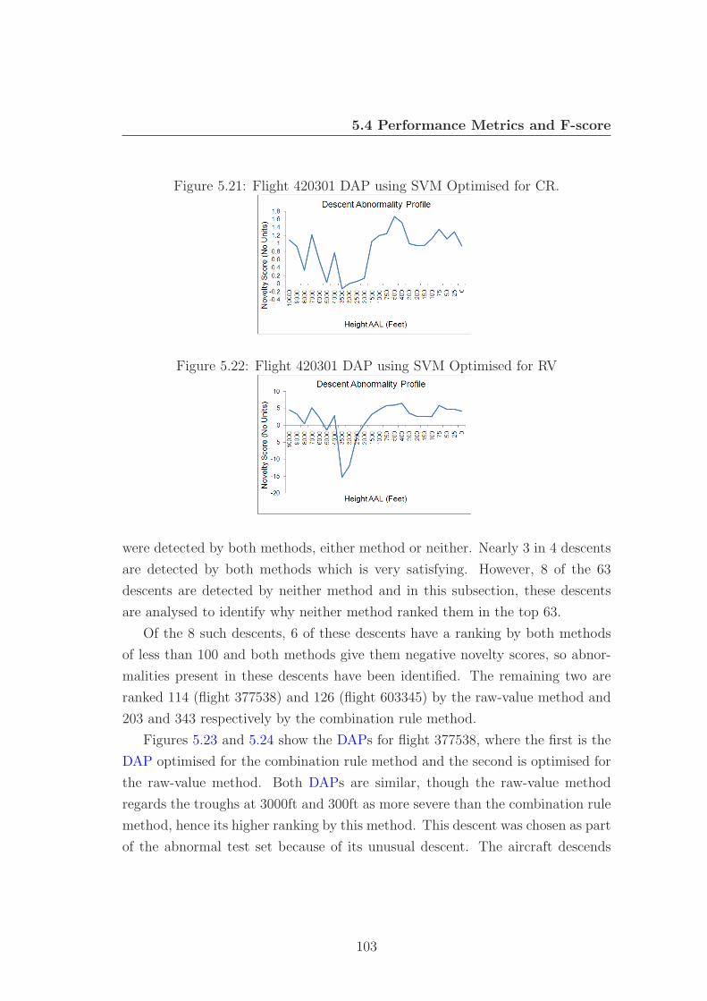
5.4 Performance Metrics and F-score
Figure 5.21: Flight 420301 DAP using SVM Optimised for CR.
Figure 5.22: Flight 420301 DAP using SVM Optimised for RV
were detected by both methods, either method or neither. Nearly 3 in 4 descents
are detected by both methods which is very satisfying. However, 8 of the 63
descents are detected by neither method and in this subsection, these descents
are analysed to identify why neither method ranked them in the top 63.
Of the 8 such descents, 6 of these descents have a ranking by both methods
of less than 100 and both methods give them negative novelty scores, so abnor-
malities present in these descents have been identified. The remaining two are
ranked 114 (flight 377538) and 126 (flight 603345) by the raw-value method and
203 and 343 respectively by the combination rule method.
Figures 5.23 and 5.24 show the DAPs for flight 377538, where the first is the
DAP optimised for the combination rule method and the second is optimised for
the raw-value method. Both DAPs are similar, though the raw-value method
regards the troughs at 3000ft and 300ft as more severe than the combination rule
method, hence its higher ranking by this method. This descent was chosen as part
of the abnormal test set because of its unusual descent. The aircraft descends
103

5.4 Performance Metrics and F-score
Figure 5.23: Flight 377538 DAP using SVM Optimised for CR.
Figure 5.24: Flight 377538 DAP using SVM Optimised for RV
Figure 5.25: Flight 603345 DAP using SVM Optimised for CR.
quickly from 7000ft to 3000ft and maintains at least 250kts to 2000ft. It has the
distance to lose this speed and does so which satisfies the stable approach criteria
by 1000ft. The trough at 300ft results from the airspeed falling below Vref and
the pitch rising to 5.4 degrees. This descent has a valid GPWS warning on it,
occurring at 363ft. Whilst the descent has some abnormality, the DAP is mostly
positive for both methods during the final approach (from 1000ft to 0ft).
Figures 5.25 and 5.26 show the DAPs produced for flight 603345 optimised for
104

5.4 Performance Metrics and F-score
Figure 5.26: Flight 603345 DAP using SVM Optimised for RV
Table 5.25: Details of False Negatives for the SVM Combination Rule Method
Method Ranked Results in the Top
63 (%)
Both 46 (73%)
None 8 (13%)
CR Only 7 (11%)
RV Only 2 (3%)
the combination rule and the raw-value methods respectively. The main abnor-
mality on this descent is a very low pitch angle at touchdown. This can be serious
if the aircraft’s nosewheel, rather than the back wheels, touched down first, as
the nosewheel was not designed to support such weight and can therefore buckle.
The DAPs for both methods are very similar, both identifying this abnormality
at 25ft and at 0ft. However the DAP for the raw-value method regards the de-
scent from 400ft to 0ft as more negative than the combination rule method. This
is because whilst both methods are using the same kernel width, the raw-value
method is set to reject 5% of the training set rather than 1%.
5.4.5 F-score
The classification in Phase 2 provides a method with which to rank descents.
Whilst it is very useful to know that a descent has a high ranking, it is also
beneficial to a flight safety officer to compare sets of descents to identify any
common trends. It would be useful to identify the heights which show the greatest
differences in novelty score and the features which cause these differences. F-score
[Chen and Lin, 2006] is a method which measures the discrimination between two
105

5.4 Performance Metrics and F-score
sets of real numbers. Consider our data set (xi)n++n
−
i=1 where n+ and n− denote
the number of positive and negative examples respectively. The F-score of the
ith feature is denoted by
F (i) ≡
(
x(+)i − xi
)2
+(
x(−)i − xi
)2
1n+−1
n+∑
k=1
(
x(+)k,i − x
(+)i
)2
+ 1n−−1
n−
∑
k=1
(
x(−)k,i − x
(−)i
)2(5.2)
where xi, x(+)i , x
(−)i are the average of the ith feature of the whole, positive,
and negative data sets, respectively; x(+)k,i is the ith feature of the kth positive
instance, and x(−)k,i is the ith feature of the kth negative instance. The numerator
provides a measure of the discrimination between the positive and negative sets.
The denominator provides a measure of the discrimination within each of the two
sets. Thus the larger the F-score value, the more likely that feature will be useful
in separating the positive from the negative examples. A disadvantage of F-score
is its inability to reveal mutual information among features.
5.4.6 Using F-score to Analyse the Data
All the descents can be represented by a feature vector of the 24 novelty values
as has already been seen. A flight safety officer might well be interested if there
are specific heights that affect the 2nd phase classification the most. Figure 5.27
shows the F-score values for each height. The two sets involved in the F-score
generation for this figure is the set of all 1455 normal descents and the set of the
63 abnormal descents (Abnormal Test Set). There are two peaks in this figure.
The first is around 6000ft to 4000ft and the second is around 500ft to 25ft. The
second peak is expected in that if the descent shows abnormalities and has made
an unstable approach, evidence of this will be seen in the final approach, perhaps
in the form of high airspeeds or low engine power settings. The first peak is more
unusual and suggests that early signs of an unstable approach may be visible at
higher altitudes.
For each height, F-score can analyse which features are most discriminative.
Figure 5.28 shows the F-scores for a selection of individual features over all the
heights. In the previous section, two peaks were noted whilst looking at the
106

5.4 Performance Metrics and F-score
Figure 5.27: F-score values for 1st Phase Novelty Scores.
0.25F-score Values 1st Phase
0.2
0.25
s (
No
Units)
F-score Values 1st Phase
0.15
0.2
0.25
alu
es (
No
Units)
F-score Values 1st Phase
0.1
0.15
0.2
0.25
ore
Va
lue
s (
No
Units)
F-score Values 1st Phase
0.05
0.1
0.15
0.2
0.25
score
Va
lue
s (
No
Units)
F-score Values 1st Phase
0
0.05
0.1
0.15
0.2
0.25
F-s
core
Va
lue
s (
No
Units)
F-score Values 1st Phase
0
0.05
0.1
0.15
0.2
0.25
10
000
90
00
80
00
70
00
60
00
50
00
40
00
35
00
30
00
25
00
20
00
15
00
10
00
750
500
400
300
200
150
100
75
50
25 0
F-s
core
Va
lue
s (
No
Units)
Height (Feet)
F-score Values 1st Phase
0
0.05
0.1
0.15
0.2
0.25
10
000
90
00
80
00
70
00
60
00
50
00
40
00
35
00
30
00
25
00
20
00
15
00
10
00
750
500
400
300
200
150
100
75
50
25 0
F-s
core
Va
lue
s (
No
Units)
Height (Feet)
F-score Values 1st Phase
0
0.05
0.1
0.15
0.2
0.25
10
000
90
00
80
00
70
00
60
00
50
00
40
00
35
00
30
00
25
00
20
00
15
00
10
00
750
500
400
300
200
150
100
75
50
25 0
F-s
core
Va
lue
s (
No
Units)
Height (Feet)
F-score Values 1st Phase
0
0.05
0.1
0.15
0.2
0.25
10
000
90
00
80
00
70
00
60
00
50
00
40
00
35
00
30
00
25
00
20
00
15
00
10
00
750
500
400
300
200
150
100
75
50
25 0
F-s
core
Va
lue
s (
No
Units)
Height (Feet)
F-score Values 1st Phase
0
0.05
0.1
0.15
0.2
0.25
10
000
90
00
80
00
70
00
60
00
50
00
40
00
35
00
30
00
25
00
20
00
15
00
10
00
750
500
400
300
200
150
100
75
50
25 0
F-s
core
Va
lue
s (
No
Units)
Height (Feet)
F-score Values 1st Phase
0
0.05
0.1
0.15
0.2
0.25
10
000
90
00
80
00
70
00
60
00
50
00
40
00
35
00
30
00
25
00
20
00
15
00
10
00
750
500
400
300
200
150
100
75
50
25 0
F-s
core
Va
lue
s (
No
Units)
Height (Feet)
F-score Values 1st Phase
0
0.05
0.1
0.15
0.2
0.25
10
000
90
00
80
00
70
00
60
00
50
00
40
00
35
00
30
00
25
00
20
00
15
00
10
00
750
500
400
300
200
150
100
75
50
25 0
F-s
core
Va
lue
s (
No
Units)
Height (Feet)
F-score Values 1st Phase
0
0.05
0.1
0.15
0.2
0.25
10
000
90
00
80
00
70
00
60
00
50
00
40
00
35
00
30
00
25
00
20
00
15
00
10
00
750
500
400
300
200
150
100
75
50
25 0
F-s
core
Va
lue
s (
No
Units)
Height (Feet)
F-score Values 1st Phase
Figure 5.28: F-score values for a selection of 1st Phase Features.
0.1F-score 1st Phase Feature Analysis
0.07
0.08
0.09
0.1
o U
nits)
F-score 1st Phase Feature Analysis
0.05
0.06
0.07
0.08
0.09
0.1
re (
No
Un
its)
F-score 1st Phase Feature Analysis
0.04
0.05
0.06
0.07
0.08
0.09
0.1
score
(N
o U
nits)
F-score 1st Phase Feature Analysis
V-VREF
0.02
0.03
0.04
0.05
0.06
0.07
0.08
0.09
0.1
F-s
core
(N
o U
nits)
F-score 1st Phase Feature Analysis
V-VREF
Pitch
0
0.01
0.02
0.03
0.04
0.05
0.06
0.07
0.08
0.09
0.1
F-s
core
(N
o U
nits)
F-score 1st Phase Feature Analysis
V-VREF
Pitch
Flap
Landing Gear0
0.01
0.02
0.03
0.04
0.05
0.06
0.07
0.08
0.09
0.1
100
00
900
0
800
0
700
0
600
0
500
0
400
0
350
0
300
0
250
0
200
0
150
0
100
0
75
0
50
0
40
0
30
0
20
0
15
0
10
0
75
50
25 0
F-s
core
(N
o U
nits)
Height (Feet)
F-score 1st Phase Feature Analysis
V-VREF
Pitch
Flap
Landing Gear0
0.01
0.02
0.03
0.04
0.05
0.06
0.07
0.08
0.09
0.1
100
00
900
0
800
0
700
0
600
0
500
0
400
0
350
0
300
0
250
0
200
0
150
0
100
0
75
0
50
0
40
0
30
0
20
0
15
0
10
0
75
50
25 0
F-s
core
(N
o U
nits)
Height (Feet)
F-score 1st Phase Feature Analysis
V-VREF
Pitch
Flap
Landing Gear0
0.01
0.02
0.03
0.04
0.05
0.06
0.07
0.08
0.09
0.1
100
00
900
0
800
0
700
0
600
0
500
0
400
0
350
0
300
0
250
0
200
0
150
0
100
0
75
0
50
0
40
0
30
0
20
0
15
0
10
0
75
50
25 0
F-s
core
(N
o U
nits)
Height (Feet)
F-score 1st Phase Feature Analysis
V-VREF
Pitch
Flap
Landing Gear0
0.01
0.02
0.03
0.04
0.05
0.06
0.07
0.08
0.09
0.1
100
00
900
0
800
0
700
0
600
0
500
0
400
0
350
0
300
0
250
0
200
0
150
0
100
0
75
0
50
0
40
0
30
0
20
0
15
0
10
0
75
50
25 0
F-s
core
(N
o U
nits)
Height (Feet)
F-score 1st Phase Feature Analysis
V-VREF
Pitch
Flap
Landing Gear0
0.01
0.02
0.03
0.04
0.05
0.06
0.07
0.08
0.09
0.1
100
00
900
0
800
0
700
0
600
0
500
0
400
0
350
0
300
0
250
0
200
0
150
0
100
0
75
0
50
0
40
0
30
0
20
0
15
0
10
0
75
50
25 0
F-s
core
(N
o U
nits)
Height (Feet)
F-score 1st Phase Feature Analysis
V-VREF
Pitch
Flap
Landing Gear0
0.01
0.02
0.03
0.04
0.05
0.06
0.07
0.08
0.09
0.1
100
00
900
0
800
0
700
0
600
0
500
0
400
0
350
0
300
0
250
0
200
0
150
0
100
0
75
0
50
0
40
0
30
0
20
0
15
0
10
0
75
50
25 0
F-s
core
(N
o U
nits)
Height (Feet)
F-score 1st Phase Feature Analysis
V-VREF
Pitch
Flap
Landing Gear0
0.01
0.02
0.03
0.04
0.05
0.06
0.07
0.08
0.09
0.1
100
00
900
0
800
0
700
0
600
0
500
0
400
0
350
0
300
0
250
0
200
0
150
0
100
0
75
0
50
0
40
0
30
0
20
0
15
0
10
0
75
50
25 0
F-s
core
(N
o U
nits)
Height (Feet)
F-score 1st Phase Feature Analysis
V-VREF
Pitch
Flap
Landing Gear0
0.01
0.02
0.03
0.04
0.05
0.06
0.07
0.08
0.09
0.1
100
00
900
0
800
0
700
0
600
0
500
0
400
0
350
0
300
0
250
0
200
0
150
0
100
0
75
0
50
0
40
0
30
0
20
0
15
0
10
0
75
50
25 0
F-s
core
(N
o U
nits)
Height (Feet)
F-score 1st Phase Feature Analysis
V-VREF
Pitch
Flap
Landing Gear
F-score values over all the heights. The second of the two peaks, at the lower
altitudes is most influenced by V-Vref and pitch, which is not surprising given
the majority of the abnormal descents have higher than average speeds on the
final approach. The first peak, at the higher altitudes, is most influenced by
flap settings and landing gear deployment. In some descents, the landing gear
is deployed in order to make the aircraft descend faster, perhaps because the
descent was later than planned. High flap settings at higher altitudes are not
usually regarded as unsafe but it is often a sign that the aircraft is making a
vectored approach and is thus able to configure the aircraft for landing at a much
higher altitude than usual.
107

5.5 Visualisation
5.5 Visualisation
5.5.1 Introduction
With great advances in processing power and ever larger data storage devices, it
is becoming increasingly possible to collect extremely large datasets. The dataset
in this thesis is a good size (1518 descents) and as such, it is possible to gain a
broad familiarity with individual descents. However, when the dataset(s) consists
of many millions of data points, it becomes virtually impossible to gain any deep
familiarity with the data unless the dataset is of a trivial nature.
Datasets containing particularly high dimensional data can be very hard to
interpret and comprehend, especially for those who do not have great experience
in data modelling. There are a variety of data visualisation tools such as clustering
or dendograms, principle component analysis, the Sammon map, Independent
Component Analysis and minimal spanning trees.
Recent innovations in visualisation algorithm development have tried to focus
on preserving the structural integrity of the original data. This implies the visu-
alisation space should be topographic in some sense. The very recent methods
have tried to extend the Sammon mapping so it is generalisable.
5.5.2 Theory
The Neuroscale algorithm [Lowe and Tipping, 1996] is an example of such a
method and is used in this section to visualise the data. The Neuroscale model
is a dimensionality reduction algorithm which uses the Sammon mapping [Sam-
mon Jr, 1969] to provide a transformation of data points from N to P dimensions
where N is greater than P . It attempts to preserve the structure of the data space
(original high-dimensional space) and retain it in the lower dimensional space. It
does this by attempting to keep the Euclidean distance between any two data
vectors as close as possible in the data space and in the latent space. The trans-
formation is generated by minimising the error function known as the Sammon
108

5.5 Visualisation
Stress Metric, given by
E =N∑
i
N∑
j>i
(d∗ij − dij)2 (5.3)
and
dij = ‖yi − yj‖ , (5.4)
d∗ij = ‖xi − xj‖ (5.5)
where d∗ij and dij represent the distance between vectors in the high dimen-
sional space the lower dimensional space respectively. A RBF neural network
is used to learn the transformation. The number of hidden nodes should be an
order of magnitude lower than the number of training vectors [Tarassenko et al.,
2008].
Throughout the rest of this thesis, Neuroscale mappings will be trained on
the normal descents and tested on the abnormal descents. Given there are 1455
normal descents and that 140 is approximately a tenth of 1455, the number of
hidden centres used will be 140.
5.5.3 Results
In this subsection, the results of the visualisation are analysed. Figure 5.29 shows
the Neuroscale visualisation of the vectors for each descent produced from the
combination rules. There is a good level of separation between the normal and
abnormal datasets and if the Euclidean distance between each datapoint and
the origin is computed, 54 of the top 63 values are from the abnormal dataset.
Furthermore, it illustrates that although there is a good level of separation be-
tween the two datasets, there are some descents in the training set that should
be regarded as abnormal.
Figure 5.30 shows the Neuroscale visualisation of the vectors for each descent
produced from the raw values from Phase 1 classification. The degree of separa-
tion is also fairly good, though if the euclidean distance between the datapoints
109

5.5 Visualisation
Figure 5.29: Neuroscale Visualisation for Combination Rule Phase 2 Results.
and origin is computed, only 45 of the top 63 values are from the abnormal
dataset.
The correlation can be computed between the Euclidean distances of the Neu-
roscale visualisations and the respective Phase 2 novelty scores. Let the Euclidean
distances be denoted by X = {xi|1 ≤ i ≤ 1518} and the Phase 2 novelty scores
be denoted by Y = {yi|1 ≤ i ≤ 1518}. Then the linear correlation between the
two variables is given by
Correl(X, Y ) =
1518∑
i=1
(xi − x) (yi − y)
√
1518∑
i=1
(xi − x)2
√
1518∑
i=1
(yi − y)2(5.6)
Table 5.26 shows the level of correlation between the Euclidean distances of the
Neuroscale visualisation and novelty scores for Phase 2 of the proposed method
110

5.5 Visualisation
Figure 5.30: Neuroscale Visualisation for Raw Value Phase 2 Results.
when both use the same SVM parameters optimised for the raw-value method
or the combination rule method. It shows there is strong negative correlation in
both cases.
111

5.5 Visualisation
Table 5.26: Correlation coefficients between the Visualisation and the Proposed Method
Method Correlation
Coefficients
Optimised for Raw-Value Method -0.867
Optimised for Combination Rule Method -0.940
112

Chapter 6
Conclusions
6.1 Introduction
This thesis has provided a solution to the difficult problem of improving flight
safety during the descent for large jet aircraft. The field of flight safety and its
existing methods was introduced in Chapter 2. In Chapter 3 novelty detection
and one class classification methods were introduced with the aim of identifying
which methods were best for the type of data at hand. The proposed method
was introduced in Chapter 4 and was described in detail. In Chapter 5 the 1st
phase results were presented along with the 2nd phase method, results, F-score
analysis and visualisation of the data.
6.2 What has been achieved?
In reviewing current flight safety methods it became clear that there are a number
of issues.
There is very little literature concerning flight data analysis and there are
a number of reasons why this is so. It could be that it has not received much
academic interest, due to the fact that real world data is likely to be confidential
and not publicly available. Therefore if research has taken place in this field, it
is likely that the vast majority was confidential and undertaken by airlines able
to afford researchers or a research department. Statistics show (Board [2010])
113

6.2 What has been achieved?
that for American airlines between 1990 and 2009, the accident rate per 200,000
departures was less than one for every year bar one. Hence it could be argued
that airlines did not feel the need to improve flight data analysis methods when
the accident rates were so low. Furthermore, current methods such as Amidan
and Ferryman [2005], are almost impossible to assess because there are no details
about the numbers of flights used, the detection rates or what they consider to
be an abnormal flight.
The event based method appears to be the most common and whilst it has
some good advantages, there are a significant number of disadvantages. It is
unable to detect exceedances if there are no events created for them. Further-
more, it is difficult to determine if there are any precursors in order to try and
explain the event and perhaps reduce its frequency which is part of the guidelines
recommended by the CAA (see section 2.3.1).
Given that airlines such as British Airways can analyse as much as 5 Giga-
bytes a day, it becomes very difficult to provide a thorough analysis of the flights,
identifying all abnormalities and their precursors (if they exist). A flight in crude
terms can be divided up into ’take off and climb’, ’cruise’ and ’descent and land-
ing’. The analysis of the event based system shows that over 70% of events occur
whilst the aircraft is in the act of descending (see section 2.5). Therefore it was
decided to focus on this region of flight as it appears to have a significant number
of abnormalities to be identified. Given that for each airport there are a set of
approaches that should be followed under normal circumstances and that ALAR
recommends that the aircraft satisfy certain conditions at 1000ft 2.6, it was con-
sidered that modelling the approach to an airfield and identifying any deviations
from the prescribed approach could be very valuable to an airline. A key mo-
tivator for this approach was the discovery that the AAIB had already made a
similar suggestion (Foundation [2004]).
Having decided on analysing the descent from considerations found in Chapter
2, it was necessary to consider what methods could be used to model an approach
to an airport. The overall goal is to detect abnormal descents and the branch
of machine learning concerned with this problem is known as ’novelty’ detection
or one class classification. The target class represents the normal flights and the
outlier class represents the abnormal flights. Chapter 3 looks at novelty detection
114

6.2 What has been achieved?
methods and one class classification methods. Perhaps the biggest difficulty in
terms of classification was the fact that identifying descents had not been, to the
best of the author’s knowledge, attempted before. Whilst the analysts at Flight
Data Services have over 150 years experience in the field of aviation and are well
versed in analysing events, they have not routinely compared individual descents.
Therefore, whilst the Abnormal Test Set contains descents with abnormalities,
it is possible that the training set (which should contain normal descents only)
may contain some abnormal descents. Therefore the classifiers used should not
be negatively impaired by the presence of abnormal descents in the training set.
Furthermore, given that the parameters occupy different numerical ranges (see
table 4.2), scaling becomes necessary so that one feature does not dominate all
the others. Therefore the classifiers should not have their performance impaired
by scaling. With these attributes in mind, the classifiers chosen were the one class
SVM, the MoG that accepts outliers in training and K-means. Furthermore, the
number of parameters to be optimised for each method is small, thus reducing
the risk of overtraining.
Section 3.4 looks at ranking systems and their applications in modern day
problems; for example, ranking bridge players and the most ’harmful’ birds to be
ingested into aircraft engines. It is clear that ranking systems are often problem
specific and rely heavily on domain knowledge. It is felt that none of these
systems are applicable to this research but it is noted that such systems can have
value. For example, it was considered surprising that blackbirds and starlings
were ranked at number 4 in terms of the risk posed to aircraft engines.
Chapter 4 and Chapter 5 introduce the method proposed in this thesis for
analysing flight data and the corresponding results. The selection of suitable
features was achieved using expert advice as to which parameters the pilots would
be monitoring during the descent. In this way it was hoped that deviations from
the airline’s SOP could be captured. The abnormal test set was also created with
advice from the staff at Flight Data Services. The test set is most unusual in its
composition (see table 4.5) give that only 32% of the descents have class 3 events.
Perhaps the most surprising feature was that it included some flights that had
no events at all. It illustrates the fact that the event system is not detecting all
abnormalities during the descent.
115

6.2 What has been achieved?
Classifiers are trained at each of the heights (see table 4.1). The output can
be plotted and the corresponding graph is known as a DAP which provides the
1st phase results. This method provides a clear visual aid to the flight safety
officer or the flight data analyst as to how the descent was flown. Regions of
abnormality are clearly highlighted and open to investigation. Furthermore, the
impact of events can usually be seen on the DAP (see figures 5.2, 5.8 and 5.14).
Key influences for phase 2 and to a lesser extent, phase 1, were the rec-
ommendation by the AAIB in Foundation [2004] and a paper by Clifton et al.
[2006] which details an intriguing method for combining information from sev-
eral combustion channels in order to determine the first early signs that unstable
combustion was taking place. Given the large numbers of flights processed, flight
safety officers and flight data analysts are clearly unable to analyse every DAP
for abnormalities. Therefore it was considered valuable to attempt to rank the
descents in order of severity and details of this approach are found in section
5.3.1. Section 5.4.3 presents the main 2nd phase results and shows that the SVM
classifier ranks the most flights from the Abnormal Test Set in the top 63 ranking
positions. It also demonstrates that the combination rule method outperforms
the raw-value method which is not too surprising given that the combination rule
method is less vulnerable to very large or very small abnormality values for a
given height.
Section 5.4.6 details the use of the feature selection tool F-score. Firstly, it is
able to identify the heights where there are the greatest differences between the
training set and the Abnormal Test Set and secondly, it is able to analyse these
heights to identify the most significant features that are causing these differences.
It was not surprising to see that features pitch and V-Vref are the most significant
at altitudes of less than 1000ft given that high speeds are a common feature of
an unstable approach. What is more unusual is that flap selection and landing
gear deployment are most significant at higher altitudes. This suggest that some
aircraft have decelerated early and are flying the approach with lower speeds and
a low flap setting in order to maintain lift. The early use of the landing gear for
some flights indicates that some aircraft are using it to descend faster because
they were a little high, or that some flights were configured ready for landing at
higher altitudes than usual.
116

6.3 Main Contributions
Section 5.5 introduces the Neuroscale visualisation algorithm which is used
to provide a visual representation of the phase 2 results. It is immediately seen
that some flights in the training set are plotted away from the main cluster of
flights centred on the origin. Section 5.4.4.1 looks at the false positives and shows
that 3 flights from the training set are ranked in positions 2, 3 and 4. The data
shows that all 3 flights had their speedbrakes deployed at altitudes under 1000ft
which is prohibited by the SOP. On further investigation it was found that
there was a fault with that parameter and the speedbrake was not deployed this
low. However, if the parameter was functioning normally, the ranking system
performed as hoped because such an event is a serious deviation from the SOP
and should be ranked highly.
6.3 Main Contributions
• The thesis highlights the apparent lack of academic research in the field of
flight data analysis and it is hoped that other researchers will be motivated
to expand and improve upon these results and conclusions.
• A new method has been introduced that identifies abnormalities and their
impact during the descent and furthermore, allows descents to be ranked
so that the descents with the most significant abnormalities are ranked in
the top positions.
• The DAP is an innovative way of showing an overview of the level of abnor-
mality during the descent. Negative regions can be clearly identified and
further studied to gain a greater understanding of that approach.
• The ranking approach has successfully identified up to 84% of the flights in
the Abnormal Test Set in the top 63 ranking positions and illustrates the
value of the combination rules.
• The proposed method is able to detect abnormalities during descents that
the event based system has not. In the Abnormal Test Set, less than a third
of the flights have level 3 events. Furthermore, some descents that had class
117

6.4 Future Work
3 events were ranked very low (see section 5.4.3), indicating that they had
no appreciable effect on the main parameters used during the descent.
• Visualisation is a valuable tool to provide a visual analysis of the rankings
produced by phase 2 and unusual descents in the training set are easily
identifiable.
• The main work of identifying a suitable model and appropriate features has
been achieved and this knowledge can be used to create models for different
aircraft types at different runways. This will enable an airline to assess how
their aircraft handle descents to different runways, take remedial actions
where required and identify any improvements in the second phase novelty
scores.
6.4 Future Work
To the best of the author’s knowledge, this is one of the first times that a large
quantity of flight data has been studied in order to improve safety. As a result,
there remains many avenues for further study.
• The study can be expanded to see how well the method performs on different
airfields.
• The method could also be applied to study the take off and climb phases
of flight to look for abnormalities.
• Different airlines flying the same aircraft type into the same airport can be
analysed and compared. Furthermore, with the agreement of all parties,
deidentified data could be shared to enable one or both airlines to improve
their SOP should it be necessary.
• The nature of flying an approach to the same airport is such that the aircraft
must fly through the same heights each time. Therefore the method can be
applied to any situation where there are a large number of repetitive actions.
For example, during a 100 metre sprint in athletics, all runners start at 0m,
118

6.4 Future Work
then pass through 10m, 20m etc and all pass through 100m. The method
could be applied to analyse how the performance of one sprinter or many
sprinters change over time. Of course, this assumes that it is possible to
extract relevant features.
119

Appendix A
Published Papers
Smart, E., Liu, H., Jesse, C. and Brown, D. (2009). Qualitative classification of
descent phases in commercial flight data. International Journal of Computational
Intelligence Studies, 1, 3749. 124
Smart, E. and Brown, D. (2009). Using novelty detection methods to identify
abnormalities in aircraft flight data. In: Proceedings of the UK Workshop on
Computational Intelligence (UKCI 2009), Nottingham, UK: University of Not-
tingham.
Smart, E. and Brown, D. (2010). Using One Class Classifiers to Diagnose
Abnormalities in Aircraft Flight Data. Intelligent Transportation Systems, IEEE
transactions on, Submitted.
120

References
ACM. Acm kdd cup - acm special interest group on knowledge discovery and
data mining, October 2010. URL http://tinyurl.com/356u4m5. Accessed on
13th August 2010. Available at http://tinyurl.com/356u4m5. 44
Aerobytes. Aerobytes fdm, 2010a. URL http://tinyurl.com/2vakxvd. Last
Accessed on 10th November 2010. Available at http://tinyurl.com/2vakxvd.
12
Aerobytes. Aerobytes foqa, 2010b. URL http://tinyurl.com/369htay. Last
Accessed on 11th November 2010. Available at http://tinyurl.com/369htay. 12
C.C. Aggarwal and P.S. Yu. Outlier detection for high dimensional data. In Pro-
ceedings of the 2001 ACM SIGMOD international conference on Management
of data, page 46. ACM, 2001. 31
Airliners. The tupolev tu-154, 2010. URL
http://www.airliners.net/aircraft-data/stats.main?id=376. Last
Accessed on 14th November 2010. 8
B.G. Amidan and T.A. Ferryman. Atypical event and typical pattern detection
within complex systems. Aerospace Conference, 2005 IEEE, pages 3620–3631,
March 2005. doi: 10.1109/AERO.2005.1559667. 13, 114
V. Barnett and T. Lewis. Outliers in statistical data. Wiley, 1994. 36
C. M. Bishop. Neural Networks for Pattern Recognition. Clarendon Press, Oxford,
1995a. 33, 35
121

REFERENCES
C.M. Bishop. Novelty detection and neural network validation. IEEE Proceedings-
Vision, Image and Signal processing, 141(4):217–222, 1994. 36
C.M. Bishop. Neural Networks for Pattern Recognition. Oxford University Press,
USA, 1995b. 41, 42, 55
National Transportation Safety Board. Aviation, 2010. URL
http://www.ntsb.gov/aviation/Table5.htm. Last Accessed on 12th
August 2010. Available from http://www.ntsb.gov/aviation/Table5.htm. 113
Boeing. 787 dreamliner, 2010. URL http://tinyurl.com/kouly. Last Accessed
on 16th November 2010. 8
D. Bradley and A. Tyrrell. Immunotronics: Hardware fault tolerance inspired
by the immune system. Evolvable Systems: From Biology to Hardware, pages
11–20, 2000. 30
C. Bregler and S.M. Omohundro. Surface learning with applications to lipreading.
Advances in neural information processing systems, pages 43–43, 1994. ISSN
1049-5258. 56
CAA. Cap 739 flight data monitoring, August 2003. URL
http://tinyurl.com/3zxtp7w. Last Accessed on 15th November 2010.
8, 9
G.A. Carpenter, S. Grossberg, and D.B. Rosen. Art 2-a: An adaptive resonance
algorithm for rapid category learning and recognition. Neural Networks, 4(4):
493–504, 1991. 55
Chambers. Abnormality. Hodder Educational Group, August 2010. URL
http://tinyurl.com/36psds4. Accessed on 12th August 2010. Available at
http://tinyurl.com/36psds4. 28
P.H. Chen, C.J. Lin, and B. Sch
”olkopf. A tutorial on ν-support vector machines. Applied Stochastic Models
in Business and Industry, 21(2):111–136, 2005. ISSN 1526-4025. 48
122

REFERENCES
Y.W. Chen and C.J. Lin. Combining svms with various feature selection strate-
gies. Studies in Fuzziness and Soft Computing, 207:315, 2006. 68, 105
L.A. Clifton, H. Yin, and Y. Zhang. Support vector machine in novelty detection
for multi-channel combustion data. Lecture Notes in Computer Science, 3973:
836, 2006. 48, 64, 116
G. Cohen, M. Hilario, H. Sax, S. Hugonnet, C. Pellegrini, and A. Geissbuhler.
An application of one-class support vector machine to nosocomial infection
detection. Studies in health technology and informatics, 107(Pt 1):716, 2004.
49
D. Dasgupta. Advances in artificial immune systems. Computational Intelligence
Magazine, IEEE, 1(4):40–49, 2007. ISSN 1556-603X. 30
D. Dasgupta, K. KrishnaKumar, D. Wong, and M. Berry. Negative selection
algorithm for aircraft fault detection. Artificial Immune Systems, pages 1–13,
2004. 30
M. Davy, F. Desobry, A. Gretton, and C. Doncarli. An online support vector
machine for abnormal events detection. Signal processing, 86(8):2009–2025,
2006. 31
R.O. Duda and P.E. Hart. Pattern classification and scene analysis. Wiley, New
York, 1973. 29, 32, 33, 73
T.V. Duong, H.H. Bui, D.Q. Phung, and S. Venkatesh. Activity recognition
and abnormality detection with the switching hidden semi-markov model. In
Computer Vision and Pattern Recognition, 2005. CVPR 2005. IEEE Computer
Society Conference on, volume 1, pages 838–845. IEEE, 2005. 31
J.C. Fayer. Vols d’essais: le Centre d’essais en vol de 1945 a 1960. E-T-A-I,
2001. ISBN 9782726885345. 7
FDS. A guide to flight data monitoring. Flight Data Services Ltd, 2010. Accessed
on 26/01/2010. Available at http://www.flightdataservices.com. 11
123

REFERENCES
Flight Safety Foundation. Stabilized approach and flare are key to
avoiding hard landings. Flight Safety Digest, August 2004. URL
http://flightsafety.org/fsd/fsd_aug04.pdf. Accessed on 4th April 2008.
Available at http://flightsafety.org/fsd/fsd aug04.pdf. 24, 27, 114, 116
FSF. Alar - approach and landing accident reduc-
tion. Flight Safety Digest, August-November 2000. URL
http://flightsafety.org/fsd/fsd_aug-nov00.pdf. 24, 27
K. Fukunaga. Introduction to Statistical Pattern Recognition. Academic Press,
1990. 28
A.B. Gardner, A.M. Krieger, G. Vachtsevanos, and B. Litt. One-class novelty
detection for seizure analysis from intracranial eeg. The Journal of Machine
Learning Research, 7:1025–1044, 2006. 50
S. Geman, E. Bienenstock, and R. Doursat. Neural networks and the
bias/variance dilemma. Neural computation, 4(1):1–58, 1992. 33
F. Girosi, M. Jones, and T. Poggio. Regularization theory and neural networks
architectures. Neural computation, 7(2):219–269, 1995. 34
A.V. Gomes, R. Voorakaranam, and A. Chatterjee. Modular fault simulation of
mixed signal circuits with fault ranking by severity. In Defect and Fault Tol-
erance in VLSI Systems, 1998. Proceedings., 1998 IEEE International Sympo-
sium on, pages 341–348. IEEE, 2002. ISBN 0818688327. 62
T. Gyimothy, R. Ferenc, and I. Siket. Empirical validation of object-oriented
metrics on open source software for fault prediction. Software Engineering,
IEEE Transactions on, 31(10):897–910, 2005. ISSN 0098-5589. 62
L.K. Hansen, S. Sigurdsson, T. Kolenda, F.A. Nielsen, U. Kjems, and J. Larsen.
Modeling text with generalizable gaussian mixtures. In Acoustics, Speech, and
Signal Processing, 2000. ICASSP’00. Proceedings. 2000 IEEE International
Conference on, volume 6, pages 3494–3497. IEEE, 2002. 41
124

REFERENCES
Paul Hayton, Bernhard Sch Olkopf, Lionel Tarassenko, and Paul Anuzis. Support
vector novelty detection applied to jet engine vibration spectra. In Advances in
Neural Information Processing Systems 13, pages 946–952. MIT Press, 2000.
50
V. Hodge and J. Austin. A survey of outlier detection methodologies. Artificial
Intelligence Review, 22(2):85–126, 2004. 31
Mike Holtom. Foqa - flight data analysis of aircraft for
flight safety. The Airline Pilots, January 2006. URL
http://tinyurl.com/3n97vy8. Accessed on 13th March 2010. Avail-
able at http://www.theairlinepilots.com/flight/foqaflightdataanalysis.htm. 10,
12, 26
F. Howard. Wilbur and Orville: A Biography of the Wright Brothers. Dover
Pubns, 1998. ISBN 0486402975. 6
T.K. Huang, C.J. Lin, and R.C. Weng. Ranking individuals by group compar-
isons. In Proceedings of the 23rd international conference on Machine learning,
pages 425–432. ACM, 2006. ISBN 1595933832. 62
ICAO. Flight safety section (fls), 2010. URL
http://www.icao.int/anb/FLS/flsannex.html. Accessed on 15th November
2010. 7
N. Japkowicz, C. Myers, and M. Gluck. A novelty detection approach to classifi-
cation. In International Joint Conference on Artificial Intelligence, volume 14,
pages 518–523. Lawrence Erlbaum Associates LTD, 1995. 31
P-. Juszczak. Learning to recognise. A study on one-class classification and
active learning. PhD thesis, Delft University of Technology, 2006. URL
http://tinyurl.com/3bfgonm. 31
S.S. Keerthi and C.J. Lin. Asymptotic behaviors of support vector machines with
Gaussian kernel. Neural computation, 15(7):1667–1689, 2003. ISSN 0899-7667.
47, 48
125

REFERENCES
L.I. Kuncheva and L.C. Jain. Designing classifier fusion systems by genetic algo-
rithms. IEEE Transactions on Evolutionary Computation, 4(4):327–336, 2000.
54
C. Lai, D.M.J. Tax, R.P.W. Duin, E. Pekalska, and P. Paclık. On combining
one-class classifiers for image database retrieval. In Proceedings of the Third In-
ternational Workshop on Multiple Classifier Systems, pages 212–221. Springer-
Verlag, 2002. 53
H. T. Lin and C. J. Lin. A study on sigmoid kernels for svm and the training
of non-psd kernels by smo-type methods. Technical report, Department of
Computer Science and Information Engineering, National Taiwan University,
2003. Available at: http://www.csie.ntu.edu.tw/ cjlin/papers/tanh.pdf. 47
D. Lowe and M. Tipping. Feed-forward neural networks and topographic map-
pings for exploratory data analysis. Neural Computing & Applications, 4(2):
83–95, 1996. ISSN 0941-0643. 108
J. Ma and S. Perkins. Time-series novelty detection using one-class support vec-
tor machines. In Proceedings of the International Joint Conference on Neural
Networks, 2003, volume 3, 2003. 31
L.M. Manevitz and M. Yousef. One-class svms for document classification. The
Journal of Machine Learning Research, 2:154, 2002. 50
M. Markou and S. Singh. Novelty detection: a reviewpart 1: statistical ap-
proaches. Signal Processing, 83(12):2481–2497, 2003a. 29, 31
M. Markou and S. Singh. Novelty detection: a reviewpart 2: neural network
based approaches. Signal Processing, 83(12):2499–2521, 2003b. 29, 31
I. Morgan, H. Liu, B. Tormos, and A. Sala. Detection and Diagnosis of Incipient
Faults in Heavy-Duty Diesel Engines. Industrial Electronics, IEEE Transac-
tions on, 57(10):3522–3532, 2010. 42
MM Moya, MW Koch, and LD Hostetler. One-class classifier networks for tar-
get recognition applications. NASA STI/Recon Technical Report N, 93:24043,
1993. 31
126

REFERENCES
S. Nandi and H.A. Toliyat. Condition monitoring and fault diagnosis of electrical
machines-a review. In Industry Applications Conference, 1999. Thirty-Fourth
IAS Annual Meeting. Conference Record of the 1999 IEEE, volume 1, pages
197–204. IEEE, 1999. ISBN 078035589X. 61
S. Nandi and H.A. Toliyat. Novel frequency-domain-based technique to detect
stator interturn faults in induction machines using stator-induced voltages after
switch-off. Industry Applications, IEEE Transactions on, 38(1):101–109, 2002.
ISSN 0093-9994. 61
NASA. Apms - aviation performance measuring system, March 2007. Accessed
on 28/08/2008. Available at http://apms.arc.nasa.gov/. 13
L. Parra, G. Deco, and S. Miesbach. Statistical independence and novelty detec-
tion with information preserving nonlinear maps. Neural Computation, 8(2):
260–269, 1996. 36, 42
E. Parzen. On estimation of a probability density function and mode. The Annals
of Mathematical Statistics, 33(3):1065–1076, 1962. 44
K. Polat and S. Guenes. A new feature selection method on classification of medi-
cal datasets: Kernel f-score feature selection. Expert Systems with Applications,
36(7):10367–10373, 2009. 68
C. Prendergast. The First Aviators. The epic of flight. Time-Life, 2004. ISBN
9781844470372. 6
S. Roberts, L. Tarassenko, J. Pardey, and D. Siegwart. A validation index for
artificial neural networks. In In Proceedings of Int. Conference on Neural Net-
works and Expert Systems in Medicine and Healthcare, page pages 2330., 1994.
36
S.J. Roberts. Novelty detection using extreme value statistics. In Vision, Image
and Signal Processing, IEE Proceedings-, volume 146, pages 124–129. IET,
2002. 29
127

REFERENCES
Jennifer Rosenberg. The first airplane crash, 2010. URL
http://tinyurl.com/4y9dssv. Last accessed 17th November 2010. 7
P.J. Rousseeuw and K. Van Driessen. A fast algorithm for the minimum co-
variance determinant estimator. Technometrics, 41(3):212–223, 1999. ISSN
0040-1706. 41
SAGEM. Analysis ground station. Sagem Dfense Securit, September 2008.
URL http://www.sagem-ds.com/ags/en/site.php?spage=00000000.
Accessed on 21/09/08. Available at http://www.sagem-
ds.com/ags/en/site.php?spage=00000000. 11
J.W. Sammon Jr. A nonlinear mapping for data structure analysis. Computers,
IEEE Transactions on, 100(5):401–409, 1969. ISSN 0018-9340. 108
B. Scholkopf, R. C. Williamson, A. J. Smola, J. Shawe-Taylor, and J. C. Platt.
Support vector method for novelty detection. In S. A. Solla, T. K. Leen, and
K.-R. Muller, editors, Advances in Neural Information Processing Systems 12,
pages 582–588, Cambridge, MA, 2000. MIT Press. 45
H. Schwenk. The diabolo classifier. Neural computation, 10(8):2175–2200, 1998.
ISSN 0899-7667. 56
H.J. Shin, D.H. Eom, and S.S. Kim. One-class support vector machines–an ap-
plication in machine fault detection and classification. Computers & Industrial
Engineering, 48(2):395–408, 2005. 50
P. Smolensky, M.C. Mozer, and D.E. Rumelhart. Mathematical perspectives on
neural networks. Lawrence Erlbaum, 1996. 34
E.J. Spinosa and A.C. de Carvalho. Support vector machines for novel class
detection in bioinformatics. Genet. Mol. Res, 4(3):608–615, 2005. 50
S. Stepney, R.E. Smith, J. Timmis, and A.M. Tyrrell. Towards a conceptual
framework for artificial immune systems. Artificial Immune Systems, pages
53–64, 2004. 30
128

REFERENCES
T. Stibor, J. Timmis, and C. Eckert. A comparative study of real-valued neg-
ative selection to statistical anomaly detection techniques. Artificial Immune
Systems, pages 262–275, 2005. 45
G. Strang. Linear algebra and its applications. New York-San Francisco-London:
Academic Press (A Subsidiary of Harcourt Brace Jovanovich, Publishers), 1980.
39
R. Subramanyam and M.S. Krishnan. Empirical analysis of ck metrics for object-
oriented design complexity: Implications for software defects. IEEE Transac-
tions on Software Engineering, pages 297–310, 2003. ISSN 0098-5589. 62
L. Tarassenko, P. Hayton, N. Cerneaz, and M. Brady. Novelty detection for the
identification of masses in mammograms. In Artificial Neural Networks, 1995.,
Fourth International Conference on, pages 442–447, 1995. 38, 45
L. Tarassenko, D.A. Clifton, P.R. Bannister, S. King, and D. King. Novelty
Detection. John Wiley and Sons, New York, 2008. 109
D.M.J. Tax. One-class classification. PhD thesis, Delft University of Technology,
http://ict.ewi.tudelft.nl/ davidt/thesis.pdf, June 2001. 29, 30, 31, 58
D.M.J. Tax. Ddtools, the data description toolbox for matlab, Dec 2009. version
1.7.3. 42
D.M.J. Tax and R.P.W Duin. Data domain description using support vectors.
In M. Verleysen, editor, Proceedings of the European Symposium on Artificial
Neural Networks 1999, pages 251–256. D.Facto, Brussel, April 1999a. 47
D.M.J. Tax and R.P.W Duin. Support vector domain description. Pattern Recog-
nition Letters, 20(11-13):1191–1199, December 1999b. 51
M.M.T. Thwin and T.S. Quah. Application of neural networks for software quality
prediction using object-oriented metrics. Journal of Systems and Software, 76
(2):147–156, 2005. ISSN 0164-1212. 62
N.R. Ullman. Elementary Statistics: An Applied Approach. Wiley, 1978. 38
129

REFERENCES
GWH van Es. Advanced Flight Data Analysis. National Aerospace Laboratory
NLR, 2002. 13
V.N. Vapnik. The Nature of Statistical Learning Theory. Springer Verlag, 2000.
45, 51
Q.H. Wang and J.R. Li. A rough set-based fault ranking prototype system for
fault diagnosis. Engineering applications of artificial intelligence, 17(8):909–
917, 2004. ISSN 0952-1976. 63
Y. Wang, J. Wong, and A. Miner. Anomaly intrusion detection using one class
svm. In Information Assurance Workshop, 2004. Proceedings from the Fifth
Annual IEEE SMC, pages 358–364. IEEE, 2005. 50
J. Weston, S. Mukherjee, O. Chapelle, M. Pontil, T. Poggio, and V. Vapnik.
Feature selection for svms. Advances in neural information processing systems,
pages 668–674, 2001. 68
Marcus Williamson. David warren: Inventor and developer of the ’black box’
flight data recorder, 2010. URL Availableathttp://tinyurl.com/3gpqake.
Last accessed 15th November 2010. 7
D.Y. Yeung and C. Chow. Parzen-window network intrusion detectors. Pattern
Recognition, 4:40385, 2002. 44
D.Y. Yeung and Y. Ding. Host-based intrusion detection using dynamic and static
behavioral models. Pattern Recognition, 36(1):229–243, 2003. ISSN 0031-3203.
30
E.J. Zakrajsek and J.A. Bissonette. Ranking the risk of wildlife species hazardous
to military aircraft. Wildlife Society Bulletin, 33(1):258–264, 2005. ISSN 0091-
7648. 63
Y. Zhou and H. Leung. Empirical analysis of object-oriented design metrics for
predicting high and low severity faults. Software Engineering, IEEE Transac-
tions on, 32(10):771–789, 2006. ISSN 0098-5589. 62
130