Embed Size (px)
Citation preview

DETAILED ANALYSIS OF PRESSURE DROP IN A LARGE DIAMETER VERTICAL
PIPE
A
THESISPRESENTED TO THE DEPARTMENT OF
PETROLEUM ENGINEERING
AFRICAN UNIVERSITY OF SCIENCE AND TECHNOLOGY
IN PARTIAL FULFILLMENT OF THE REQUIREMENTS
FOR THE DEGREE OF
MASTER OF SCIENCE
By
NWACHUKWU KIZITO CHIBUIKE, B.Eng.(Hons.)
Abuja, Nigeria
December 2014
DETAILED ANALYSIS OF PRESSURE DROP IN A LARGE DIAMETER VERTICAL
PIPE
By
NWACHUKWU KIZITO CHIBUIKE, B.Eng.(Hons.)
A THESIS APPROVED BY THE PETROLEUM ENGINNERING DEPARTMENT

RECOMMENDED: …………………………………………
Supervisor, Dr. Mukhtar Abdulkadir
…………………………………………..
Head, Department of Petroleum Engineering
APPROVED: ……………………………………….....
Chief Academic Officer
…………………………….
Date
ABSTRACT
With the ever increasing need to optimize production, the accurate understanding of the
mechanics of multi-phase flow and its effect on the pressure drop along the oil-well flow
string is becoming more pertinent. The efficient design of gas-lift pump, electric submersible
pumps, separators, flow strings and other production equipment depends on the accurate
prediction of the pressure drop along the flow pipe. Pressure is the energy of the
2

reservoir/well and it is crucial to understand how a change in fluid properties, flow conditions
and pipe geometric properties affect this important parameter in the oil and gas industry.
Extensive work on this subject has been done by numerous investigators albeit in small
diameter pipes. Reliance on the empirical correlations from this investigators has been
somewhat misleading in modelling pressure drop in large diameter pipes (usually >100 mm)
because of the limitations imposed by the diameter at which they were developed and the
range of data and conditions used in deriving them.
In this work, experimental data from the experimental study by Dr. Mukhtar Abdulkadir was
used as the data source. The gas velocities, liquid velocities, film fraction, gas and liquid
properties and the pipe geometric properties from the above mentioned experiment were used
to model the frictional and total pressure drop from six correlations. Results were analyzed
and compared with the experimental results.
ACKNOWLEDGEMENT
I would like to thank in a special way my sister and mentor Engr. Angela Nwachukwu,
without her I won’t be here. She has shown more than a sister’s love to me and I will be
forever indebted to her. I appreciate my dearest mum Mrs. Rose Nwachukwu and all my
siblings for being there for me always.
I want to use this opportunity to express my gratitude to Dr. Mukhtar Abdulkadir for his
continuous support and motivation throughout this work. His guidance was invaluable to the
3

success of this work. My appreciations also goes to all the lecturers for helping me in one way
or the other in acquiring the bank of knowledge and information required in accomplishing
this task.
I appreciate the support from all AUST students, all the masters and PhD students. Special
mention goes to Azeko Salifu Tahiru who assisted me in using the statistical software,
Minitab-16, used in some of my analysis and Bruno S. Dandogbessi for his numerous advices.
The friendship and support I got from all of you kept me going.
DEDICATIONThis work is dedicated to the almighty God without whom nothing is possible. I also dedicate
this to my lovely family for their support and encouragement.
4

TABLE OF CONTENTS
1.1 General introduction.....................................................................................................9
1.2 Problem statement.......................................................................................................12
1.3 Aims and Objectives...................................................................................................12
1.3.1 Aim..................................................................................................................12
1.32 Objective..........................................................................................................12
1.4 Structure of the thesis......................................................................................................13
2.1 Introduction.................................................................................................................15
2.2 Void Fraction and Liquid Holdup................................................................................24
2.3 Flow Regimes.............................................................................................................25
Figure (2.31): A typical flow pattern map for vertical upward gas-oil flow....26
Figure (2.341): Flow patterns in vertical upward flow....................................29
2.4 Flow pattern maps.......................................................................................................29
5

Figure (2.42): Flow regime map showing the different flow regimes.............31
Figure (2.43): Flow evolution of a multiphase fluid along a flow string........32
2.5 Pressure Drop determination.......................................................................................33
3.1 Large Scale Two-phase Flow Closed Loop.................................................................36
Table (3.1): Properties of the fluids at a pressure of 3 bar (absolute) and at the operating temperature of 20oC............................................................37
3.2 Pressure Drop Measurement.......................................................................................40
3.3 Visual studies..............................................................................................................41
3.4 Experimental conditions.............................................................................................42
4.1 Introduction.................................................................................................................44
4.2 Time-varying pressure drop........................................................................................45
Figure (4.30): Total pressure drop as a function of gas superficial velocity. . .50
Figure (4.31): Total pressure drop as a function of mixture superficial velocities.. .52
Figure (4.32): Total pressure drop as a function of gas mass flux (Gg)..........52
Figure (4.33): Pressure drop as a function of liquid film fraction...................53
4.4 Measured frictional pressure drop...............................................................................54
Figure (4.40): Measured frictional pressure drop as a function of gas superficial velocity.............................................................................................................55
4.5 sensitivity analysis on the effect of diameter on the frictional pressure drop.............55
Figure 4.50: Effect of pipe diameter on frictional pressure drop for Friedel (1979) correlation........................................................................................................56
Figure 4.51: Effect of pipe diameter on frictional pressure drop for Beggs and Brill (1973) correlation............................................................................................57
Figure 4.52: Effect of pipe diameter on frictional pressure drop for Poettmann and Carpenter (1952) correlation............................................................................57
Figure 4.54: Effect of pipe diameter on frictional pressure drop for Modified Hagedorn and Brown (1964) correlation.........................................................58
Figure 4.55: Effect of pipe diameter on frictional pressure drop for Baxendel and Thomas (1961) correlation..............................................................................59
4.6 Comparison between measured and calculated frictional pressure drop....................59
4.7 Comparison of experimental total pressure drop with results from empirical correlations........................................................................................................................61
Figure (4.711): Cross plot of pressure drop for all the selected correlations...63
4.8 Regression analysis using minitab-16 statistical software..........................................65
Figure (4.81): Regression analysis of experimental and calculated results.....65
Figure (4.82): Diagnostic report of measured and calculated results..............66
Table (4.2): Descriptive statistics report of measured and calculated results....67
6

Figure (4.84): Comparison of experimental and calculated pressure drop result.....68
5.1 Conclusion..................................................................................................................69
5.2 Recommendation........................................................................................................70
5.3 Future work.................................................................................................................70
Figure A1: Friction factor chat for different empirical correlations................81
Table B1: Fluid and Pipe geometric properties...................................82Table B1: Friedel pressure drop modelling procedure........................83.............................................................................................................84
.............................................................................................................85Table B2: Beggs and Brill pressure drop modelling procedure..........85.............................................................................................................86Table B3: Poettmann and Carpenter modelling procedure..................86Table B4: Chisholm modelling procedure...........................................87Table B5: Modified Hagedorn and Brown modelling procedure........88Table B6: Baxendel and Thomas modelling procedure......................90
CHAPTER ONE
INTRODUCTION
1.1 General introduction
Profitable production of oil and gas fields relies on accurate prediction of the multi-phase well
flow. The determination of flowing bottom-hole pressure (BHP) in oil wells is very important
to petroleum engineers. It helps in designing production tubing, determination of artificial lift
requirements and in many other production engineering aspects such as avoiding producing a
well below its bubble point in the sand-face to maintain completion stability around the
7

wellbore (Ahmed, 2011). Well fluids above bubble point pressure exist as a single phase as it
is being produced from the reservoir. However, as they navigate their way through the
network of interconnected pores in the reservoir to the wellbore, there is a continuous
reduction in pressure as overburden stress is gradually reduced. This phenomenon leads to the
liberation of the entrained gas. As the single-phase fluid rises in the tubing, a critical point is
reached where some of the gases begin to come out of solution along the length of the pipe. In
other words, it changes from single-phase flow to multi-phase flow.
This leads to some level of complexity as regards to the identification of the physical
properties of the individual phases, the flow pattern, the relative volume occupied by the
separate phases inside the pipe, and most importantly the implication of the phase separation
on the pressure drop along the well tubing string.
Although most if not all calculations for flow lines in multiphase production systems have
been and continue to be based on empirical correlations, there is now a strong tendency to
introduce more physically based (so called mechanistic) approaches to supplement if not
replace correlations. This is because the latter are well known for their unreliability when
applied to systems operating under conditions different to those from which the correlations
are derived; such conditions encompass: pressure, temperature, fluid properties and pipe
diameter. Furthermore, correlations exist for limited geometrical configurations (i.e. vertical
or horizontal pipes) and simple physical phenomena (no mass transfer between phases,
constant temperature, etc.). With the advent of more complex production systems involving
deviated wells as well as the move to exploit gas condensate resources the production of
which will inevitably involve strong mass transfer effects, calculation methods will be
required to account for such complexities. The use or extension of existing correlations to
8

such systems will therefore be fraught with uncertainties if at all possible (Issa and Tang,
1991).
Petroleum Engineers need to predict pressure drops in oil and gas wells for the following
reasons:
1) To construct "lift-curves", which are tables or plots of flow-rate versus bottom hole-
pressure, used to predict well flow-rates.
2) To select the appropriate tubing size. If the tubing diameter is too large, the well acts as a
gas-liquid separator and a flow conduit, and the excessive slippage results in needlessly high
bottom hole pressures. However, tubing which is too small will cause excessive frictional
pressure drops.
3) To design artificial lift completions such as electric submersible pumps, jet pumps or gas
lift.
(Pucknel- et al, 1993).
Pressure drop along the vertical tubing comes in two main components:
Frictional drop and
Hydrostatic drop
The acceleration component of the pressure drop is usually negligible in adiabatic flows, and
hence would not be considered in this work.
In the lower portion of the flow string pressure drop due to gravity is much more
predominant, meanwhile frictional pressure drop accounts for most of the total pressure drop
9

a column of multiphase fluid experiences along any flow conduit in the annular flow regime.
Though this is particularly valid for small diameter pipes.
The ability to predict the variation of pressure with elevation along the length of tubing for
known conditions of flow would provide a means of evaluating the effects of tubing size, flow
rates and a host of other variables on flowing wells and would be particularly useful in
designing gas-lift installations (Poettmann & Carpenter, 1952).
Considerable work has been done on the laws governing the multiphase flow of liquid and gas
mixtures in vertical pipes but no satisfactory solution has been found applicable to flowing oil
wells and gas-lift wells. There has been a lot of investigation on small diameter pipes but
there exist a lack of experimental data in large diameter vertical pipes, i.e., in pipe sizes
similar or close to those typical of industry applications and especially on important
parameters such as pressure drop which is known as a key design parameter. Many empirical
correlations have been developed in the past from the experimental data for predicting two-
phase pressure gradient which differ in the manner used to calculate these three components
above of the total pressure drop (Hewitt, 1982a, Brill and Beggs, 1991 and Azzopardi, 2006).
It is worth mentioning that even with many empirical correlations and models that are
available in literature they appear not to be valid over a very wide range of gas and liquid
flow rates, physical properties and pipe diameters. Therefore researchers normally test the
performance of these methods of prediction with the experimental data that are available to
them.
1.2 Problem statement
10

With a plethora of correlations trying to model the two-phase flow of oil and gas wells
through a conduit, it is pertinent to know the ones that come close to the actual physical
measurements. The main drive in this work is to:
Analyze the data on the experiment carried out by Mukhtar Abdulkadir which
comprises of total pressure drop, liquid film fraction and gas and liquid superficial
velocities.
Compare the total pressure drop extracted from this experimental data with the
frictional pressure drop calculated from selected empirical correlations.
1.3 Aims and Objectives
1.3.1 AimThe aim of the study is to carry out a detailed analysis of pressure drop in a large diameter
vertical pipe.
1.32 ObjectiveTo achieve this aim, the following objectives will be met:
11

To obtain raw experimental data concerned with total pressure drop on churn-annular
flows in 127 mm diameter, 11 m length vertical pipe over a wide range of gas and
liquid superficial velocities. This will be achieved by processing raw data obtained
from an experiment conducted by Dr. Mukhtar Abdulkadir.
To compare the data obtained with those available in the literature for smaller pipes so
as to investigate the effect of pipe diameter on total pressure drop.
To analyses the frictional pressure drops correlations of various investigators. The
correlations chosen for the analysis include Poettmann and Carpenter (1952), Beggs
and Brill (1973), Friedel (1979), modified Hagedorn and Brown (1964), Baxendel and
Thomas (1961) and Chisholm (1973) frictional pressure drop correlations.
To make a comparison between the predicted pressure drop and that obtained from
experimental observation (measured pressure drop) using various statistical analysis
techniques.
1.4 Structure of the thesis
Chapter provides the introduction, the aims and objectives of this work
Chapter two of this thesis provides a review of some important literatures on this
topic. It provides the methods and procedure in which different authors and
investigators looked at flow dynamics in vertical multi-phase flow as regards to
pressure drop prediction.
12

Chapter three focuses on the experimental/design techniques carried out based on the
experiment carried out by Dr. Mukhtar Abdulkadir on 127mm (0.127m) diameter, 11
m vertical pipe. It shows the procedure that was taken in deriving the total pressure
drop, the void fraction (film fraction) for each liquid and gas flow-rates. Finally, in
chapter three pressure drop using different correlations were determined as an
alternative to experimental technique. This is important for comparative purposes and
to determine the best correlation that would fit the conditions at which the experiment
was carried out.
Chapter four shows all the analysis carried out to compare the pressure drop derived
from experiment with the pressure drop from selected pressure drop correlations.
Various forms of statistical analysis techniques were used to compare and contrast the
pressure drop correlations in order to determine the best out of the lot.
Chapter five is conclusion and recommendation.
CHAPTER TWO
LITERATURE REVIEW
2.1 Introduction
The prediction of pressure drop in two-phase flow in vertical tubing has received numerous
attention from several investigators. Most of the correlations developed, unfortunately, are
limited in their application due to the range of data used in deriving them. And currently there
is scarcity of correlations in literature on pipes with diameter greater than 100 mm but a look
13
at the correlations on smaller diameter pipes can give us a hint on the effect of pipe diameter
on two-phase pressure drop in vertical pipes.
Aziz et al (2001), developed a sound mechanistically-based prediction method for the flow
pattern encountered in oil wells- those where the oil is the continuous phase, i.e., the single
phase, the bubble and slug flow patterns. They argued that all methods for the prediction of
the relationship between the pressure gradient, the flow rates, the fluid properties and the
geometry of the flow duct involve one form or another of the mechanical energy equation. For
a small elevation change, ΔZ, the equation maybe written as equation (2.111).
They developed a calculation method with the concept described. The proposed method,
based on mechanical considerations, permit ready identification of the flow pattern, and the
calculation of the in-situ void fraction of the gas phase and the pressure gradient.
The predicted pressure drop compares favorably with measured values in 44 of the 48 wells
for which adequate data are reported.
14

Hagedorn and Brown (1964) method is based on data obtained from a 1500 feet deep
vertical experimental well. Air was the gas phase and four different liquids were used: water
and crude oil of viscosities of about 10, 30 and 110 cP. Tubing of about 1.0, 1.25 and 1.5 in.
nominal diameters were used. However, Hagedorn and Brown (1964) did not measure liquid
hold-up, rather they developed a pressure gradient equation that, after assuming a friction-
factor correlation permitted the calculation of pseudo liquid hold-up values for each test to
match measured pressure gradients.
Hagedorn and Brown developed a pressure gradient for vertical multi-phase flow using
equation (2.115).
Gray (1978) developed a method to determine pressure gradient in a vertical well that also
produces condensate fluids or water. A total of 108 well-test data were used to develop the
empirical correlation. Of these sets, 88 were obtained on wells reportedly producing free
liquids.
Gray proposed equation (2.115) to predict pressure gradient for two-phase flow in a vertical
gas well.
Fancher et al (1963) developed a correlation which is based on Poettmann and Carpenter
(1952)’s method. An energy balance between any two points in the flow string in which the
flowing fluid was treated as a single homogeneous fluid was developed as a basis for their
correlation. The irreversible energy losses were incorporated in a Fanning-type friction factor
term. A correlation was developed by back-calculating the friction term from field data and
plotting it against the numerator of the Reynolds number. Viscosity effects were not included
15

in their correlation due to the high degree of turbulence of both phases. Viscous shear is
negligible if both phases are in high degree of turbulence.
In their work, the original Poettmann and Carpenter (1952) correlation was extended to
cover the lower density ranges (in particular less than 10 lb. /cu-Ft. for 2-inch tubing), which
Poettmann stated was outside the range of their original data. This lower density range was
further correlated by using the producing gas-liquid-ratio as an additional parameter.
The irreversible energy loss term was evaluated by calculation using field data to determine
the pressure gradient from equation (2.117)
They plotted the fanning-type friction factor against the numerator of the Reynolds number.
The scattering of points in this correlation shows that an important parameter(s) was/were
neglected. They then employed the gas-liquid-ratio as an additional parameter, and a
correlation was developed between the Fanning friction factor and the numerator of the
Reynolds number for three ranges of gas-liquid-ratios.
In comparing their correlation to that of Poettmann and Carpenter (1952), they concluded that
Poettmann and Carpenter correlation shows excellent agreement at high flow rates, but results
in large deviation at low flow rates and low density ranges.
Chierici et al (1974) examined the pressure drop and flow regimes in a vertical flowing oil
well. Starting from the mechanical energy balance equation, they expressed the elementary
pressure drop, dp, in a vertical well as follows:
By making some approximations in evaluating the acceleration gradient, VdV, which is
almost negligible, equation (2.119) was obtained:
16
They grouped the various ways a gas-liquid mixture can flow in a vertical pipe into three
main flow regimes; that is, bubble-plug flow, slug-froth flow, and mist flow. A transition flow
exists between the last two flow regimes.
The frictional loss gradient, is calculated according to the classical equation;
Where the friction factor, f, is obtained by entering the Moody diagram with the appropriate
NRe and ε/dh values. What density, velocity and Reynolds number are to be used depends on
the flow regime mentioned above.
In their paper, Hasan and Kabir (1988) examined the void fractions for different flow
regimes (bubbly, slug, churn and annular flow regimes), the transition criteria and the pressure
gradient predictions. The void fraction and pressure gradient predictions of the theory
presented in their paper for vertical up-flow of two-phase fluids are compared with published
data from diverse sources. The predictions of the proposed theory were plotted against the
void fraction data of Beggs and Brill (1973) for vertical systems. Beggs and Brill’s data were
gathered with air/water in 1.5- and 1-in. (3.8- and 2.5-cm) pipes at 4- to 7-atm (405- to 709-
kPa) pressures and 50 to 1000F (10 to 380F) temperatures. The agreement between the data
and the prediction were excellent for all flow regimes except churn flow. Their theory appears
to over-estimate void fraction during churn flow slightly, suggesting a somewhat higher value
of C1 than is usually used. However, they also observed that the highly fluctuating nature of
churn flow makes accurate data gathering difficult.
Their study presents a model for predicting flow behavior of two-phase gas/oil mixtures in
vertical oil wells. The major advantage of the proposed method is that it is based on the
physical behavior of the flow and therefore is more reliable than available correlation under
17

diverse production conditions. They used data from various sources to verify the accuracy of
the model.
Specifically the model is capable of predicting flow regime, void fraction, and pressure drop
at any point in the flow string.
Pucknell et al (1993) evaluated two of a number of published mechanistic models – one by
Ansari (1994) and the other by Hasan and Kabir (1988).
The objective of their work was to compare the Ansari and the Hasan & Kabir methods
against the traditional multi-phase correlations. The following performance measures were
used, based on the practical application of these models:
1) When predicted pressure drops are compared with measurements made in oil and gas
fields, the multiphase model should give accurate results across the full range of producing
conditions.
2) In combination with other information, the method should accurately predict when a well
will cease to flow stably. In some cases, the requirements for "kicking off', adding artificial
lift or recompleting with smaller tubing later in the well's life can be very important.
3) The method should not contain any discontinuities which result in sudden changes in
pressure as a result of small changes in flow-rate or some other parameter.
4) The model should not be prone to numerical convergence problems.
With the oil flow-rate, water-cut, gas-oil-ratio and pressure at the wellhead readily available,
they obtained a bottom-hole pressure through well-tests (just prior to pressure buildup) and
production logging. The two sources of data were used in their study.
18

246 measurements of bottom hole flowing pressure were obtained, together with the required
ancillary data, from 8 producing fields. Virtually all the data were from deviated wells with
tubing of between 3 1/2" and 7".
None of these measurements was available during the development of any of the multiphase
models considered, so their use represents a completely independent test.
In the result, no model gives the best results for all fields. The variability in performance can
be extreme. For example, Duns and Ros (1963) gives good results in oilfield B with absolute
errors of under
3%, however the same method gives an error of119% in gas field A. The results support the
accepted practice of determining which correlation gives the most accurate predictions of
bottom-hole pressure in each field. That method is then used to predict future field
performance.
Despite the development of new mechanistic models, no single method gives accurate
predictions of bottom hole flowing pressures in all fields.
Takacs (2001) examined the problem of predicting multiphase pressure drops in oil wells by
analyzing the findings of all previously published evaluations. Based on these, the following
main conclusions can be drawn:
None of the available vertical multiphase pressure drop calculation models is generally
applicable because their prediction errors may considerably vary in the different
ranges of the flow parameters.
There is no “over-all best” calculation method, and all efforts to find one are deemed
to fail.
19

In spite of the claims found in the literature, the introduction of mechanistic models did not
deliver a breakthrough yet because their accuracy does not substantially exceed that of the
empirical ones.
Based on a sufficiently great number of experimental data from the oilfield considered, one
can determine the optimum pressure drop prediction method for that field.
Reinicke et al (1987) investigated more than 15 correlations and combinations of correlations
in order to identify the best method for prediction of pressure loss in deep, high-water-cut gas
wells. These correlations are categorized into four groups: single-phase correlations, two-
phase correlations based on the assumption that gas and liquid phases travel at the same
velocity (no-slip, no-flow-regime consideration), two-phase correlations that consider
slippage between the phases but no-flow regimes, and two-phase correlations that consider
both slip and flow regimes.
A main program was written and the various pressure prediction methods and fluid-property
correlations incorporated as subroutines. These routines were taken from published sources
whenever possible (e.g., Brill and Beggs, 1973) and supplemented by routines developed in-
house only where necessary. The program allows calculations from either top to bottom or
bottom to top. The total length of the wellbore can be sectioned to handle changes in
tubing/casing size, wellbore deviation, and pipe roughness. Each of these sections can be
divided further into increments in which the pressure-gradient equation is solved for either
pressure or length.
Khasanov et al (2007) developed an analytical void fraction expressions for each of the flow
regime considered and used in well optimization cycle. Such expressions enable explicit
20

pressure versus depth dependence to be developed as soon as the proper simplifying
assumption on PVT properties are made (for example, the linear dependence for solution gas-
oil-ratio on pressure). The evaluation of the proposed model was performed by comparing the
predicted pressure drop to the measured one according to the wells from TUFFP databank for
four mechanistic models. The models involved in comparison are: Ansari mechanistic model,
Unified mechanistic model, Hasan and Kabir (1988). The pressure drop was calculated with
the use of the above three mechanistic model plus the proposed model. A new model for void
fraction and pressure gradient prediction for vertical and slightly deviated wells was
developed based on drift-flux approach. The model was evaluated using TUFFP databank as
well as Rosneft field data. Evaluation showed that in comparison with mechanistic models,
the proposed model enables the calculation of pressure with comparable accuracy, and less
calculation resources required. Due to simplicity of void fraction expression provided by drift-
flux approach, this approach allows calculating pressure gradient for a great number of wells
simultaneously which is essential in production optimization.
Poettmann and (1952) in their classic paper described a method of predicting the pressure
transverse of flowing oil wells and gas-lift wells. The method is based on a field data from a
large number of flowing and gas-lift wells operating over a wide range of conditions. As in
any correlation, there are definite limitations and range of operations to which the correlation
can be applied. The correlation is based on 2-, 2 ½-, and 3-in. diameter nominal size tubing;
gas-liquid ratios of up to 5,000 cu-ft. of gas per barrel of liquid; liquid rates from 60 bbl. to
1,500 total liquid per day; water-oil ratio of 56 bbl. of water per bbl. of oil; oil gravities from
30 API to 56 API; and well depths to 11,000 ft.
21

The procedure developed permits the calculation of the bottom-hole pressure of flowing
knowing only surface data; and, in the case of gas-lift wells, it permits calculation of the depth
at which to inject the gas, the pressure at which to inject the gas, the rate at which to inject the
gas, the ideal horsepower requirements necessary to lift the oil, and the effect of production
rate and tubing size on these quantities.
In order to establish an idea of the reliability of the correlation, they compared the overall
pressure gradients with field-measured gradients. The agreement between observed and
calculated results was good. The algebraic average deviation for all the data was +1.8 percent
and the standard deviation from the algebraic average was 8.3 percent.
2.2 Void Fraction and Liquid Holdup
In the flow of oil well fluids from the reservoir, there is a gradual decrease in the pressure
acting on the fluid. Phase separation gradually occurs as the confining pressure is gradually
removed. When we have multiple phases passing through a cross-section of the pipe, each
phase can obviously not cover more than a fraction of the area. If, for instance, a fourth of the
cross-section is occupied by gas, we say the gas area fraction (or the volume fraction, since
volume corresponds to area if the length of that volume is infinitely small) or simply the void
fraction is 0.25. If the remaining area is occupied by liquid, the liquid hold-up (liquid fraction)
has to be 1 - 0.25 = 0.75. The void fraction and liquid holdup is a function of the relative
liquid and gas velocities and flow rates.
22

The void fraction along the length of the pipe varies from zero when the fluid is still in single
phase to over 0.9 in annular flow. This has a significant effect on the pressure drop along the
vertical flow string.
There are different correlations used in estimating void fractions
Where: Equation (2.21) clearly suggests that accurate estimation of the gas void fraction is
essential to the hydrostatic head computation that accounts for most of the pressure drop -
greater than 90 % at low flow rates.
2.3 Flow Regimes
When a gas and a liquid are forced to flow together inside a pipe, there are at least 7 different
geometrical configurations, or flow regimes that are observed to occur. These spatial
configurations of the gas and liquid phases affect the pressure losses along the flow string in
one way or the other. The flow regime depends on the fluid properties, the size of the conduit
and the flow rates of each of the phases. The flow regime can also depend on the
configuration of the inlet; the flow regime may take some distance to develop and it can
change with distance as (perhaps) the pressure, which affects the gas density, changes. For
fixed fluid properties and conduit, the flow rates are the independent variables that when
adjusted will often lead to changes in the flow regime. There is no sharp changes in the flow
regime, hence there exists flow regime transitions (McQuillen et al).
The boundaries between the various flow patterns in a flow pattern map occur because a
regime becomes unstable as the boundary is approached and growth of this instability causes
transition to another flow pattern. Like the laminar-to-turbulent transition in single phase flow,
these multiphase transitions can be rather unpredictable since they may depend on otherwise
23

minor features of the flow, such as the roughness of the walls or the entrance conditions.
Hence, the flow pattern boundaries are not distinctive lines but more poorly defined transition
zones (www.cco.caltech.edu/~brennen/multiph/chap7.pdf). Figure (2.31) shows the vertical
flow regime map of Hewitt and Roberts (1969) for flow in a 3.2cm diameter tube, validated
for both air/water flow at atmospheric pressure and steam/water flow at high pressure.
Figure (2.31): A typical flow pattern map for vertical upward gas-oil flow.
2.3.1 Bubbly flow: At low gas-fractions, the liquid is continuous and the gas exists as
individual bubbles. In the bubble flow pattern, the liquid phase almost completely fills the
pipe and the gas is present in the liquid as small bubbles and is randomly distributed. The
diameters of the bubbles vary randomly. Also the velocities of the bubbles are different
24

because of the respective diameters. This type of flow occurs at low turbulence and also at
relatively low liquid rates. Some authors make the distinction between homogeneous (or
dispersed) and heterogeneous (or discrete) bubbly flow. Homogeneous flow occurs at low
voidages, where the bubble size distribution (BSD) is narrow and there exists little interaction
between bubbles, while with increasing gas-fraction the distribution broadens and bubble
coalescence and break-up begin to occur. The boundary between homogeneous and
heterogeneous bubbly flow is not well defined.
2.3.2 Slug flow: Slug flow is characterized by series of slug units. Each unit is composed of
gas pocket called a Taylor bubble, a plug of liquid called a slug, and a film of liquid around
the Taylor bubble flowing downward relative to the Taylor bubble. The Taylor bubble is an
axially symmetrical, bullet-shaped gas pocket that occupies almost the pipe’s entire cross-
section. As the gas-fraction increases, bubble coalescence becomes more prolific and the
mean bubble size increases until slugs form which approach the diameter of the column.
2.3.3 Churn flow: Churn flow is the chaotic flow of gas and liquid in which the shape of both
the Taylor bubble and the liquid slugs are distorted. It results from the instability of the Taylor
bubbles caused by increased void fraction and gas velocity. Neither phases appear to be
continuous. The continuity of the liquid in the slug is represented by a high local gas
concentration. An oscillatory or alternating direction of motion in the liquid phase is typical of
churn flow. Churn flow with its characteristic oscillations is an important pattern and, often
covering a fairly wide range of gas flow rate. At its higher range of gas velocity, the liquid
consists mainly of a thick film on the pipe wall covered with large waves. Therefore, in that
25
sense the term semi-annular can be used for this flow pattern. However, researchers, e. g.,
Hewitt and Hall-Taylor (1970), prefer the more general term "churn" to cover the whole
region.
2.3.4 Annular flow: Annular flow is characterized by axial continuity of the gas phase in a
central core with the liquid flowing upwards, both as thin film along the pipe wall and as
dispersed droplets in the core. At high gas flow rates more liquid become dispersed in the
core, leaving a very thin liquid film flowing along the wall. According to Costigan and
Whalley (1997), the annular type flow in vertical pipes occurs at gas void fractions above 0.8.
The interfacial shear stress acting at the core/film interphase and the amount of entrained
liquid in the core are important parameters in annular flow.
Fig (2.341) represents the geometrical configuration of the different flow regions encountered
in a poly-phasic flow.
26

Figure (2.341): Flow patterns in vertical upward flow
2.4 Flow pattern maps
Flow pattern map is one of the most important things to consider in two-phase flow design
problems. For some of the simpler flows, such as those in vertical or horizontal pipes, a
substantial number of investigations have been conducted to determine the dependence of the
flow pattern on component volume fluxes, (JA, JB), on volume fraction and on the fluid
properties such as density, viscosity, and surface tension. The results are often displayed in the
form of a flow pattern map that identifies the flow patterns occurring in various parts of a
parameter space defined by the component flow rates. The flow rates used may be the volume
fluxes, mass fluxes, momentum fluxes, or other similar quantities depending on the
investigator. Summaries of these flow pattern studies and the various empirical laws extracted
from them are a common feature in reviews of multiphase flow.
One of the basic fluid mechanical problems is that these maps are often dimensional and
therefore apply only to the specific pipe sizes and fluids employed by the investigator. A
number of investigators (for example Baker 1954, Schicht 1969 or Weisman and Kang 1981)
have attempted to find generalized coordinates that would allow the map to cover different
fluids and pipes of different sizes. However, such generalizations can only have limited value
because several transitions are represented in most flow pattern maps and the corresponding
instabilities are governed by different sets of fluid properties. Even for the simplest duct
geometries, there exist no universal, dimensionless flow pattern maps that incorporate the full,
parametric dependence of the boundaries on the fluid characteristics. Moreover, the implicit
27

assumption is often made that there exists a unique flow pattern for given fluids with given
flow rate.
In summary, there remain many challenges associated with a fundamental understanding of
flow patterns in multiphase flow and considerable research is necessary before reliable design
tools become available. Figure (2.41) and figure (2.42) depicts how the various flow regimes
are represented in a flow pattern maps.
Figure (2.41): Flow Pattern Map showing boundary and transition of flow regime.
(Source: http:// www.google.com/imgres?q=flow+pattern+map&hl)
Figure (2.42): Flow regime map showing the different flow regimes.
28

Most general two-phase flow correlations and models suffer from a lack of physically-sound
flow regime models because characterization of the different hydrodynamic properties is a
highly complex task. Therefore, the flow regimes form the bed rock of many of the proposed
two-phase flow models. “Parametric relationships are developed, valid for a limited range of
flow patterns, to describe the dependence of the predicted/measured flow properties on the
consequent flow conditions. It is wholly assumed that the flow regime present is either clearly
recognizable or known a priori” Abdulkadir (2011). Figure (2.43) shows the flow evolution
as a single phase flow changes to multi-phase flow as the fluid confining pressure is reduced
along the flow string.
Figure (2.43): Flow evolution of a multiphase fluid along a flow string. (authors.library.caltech.edu/25021/1/chap7.pdf)
29

2.5 Pressure Drop determination
The fundamental equation for a pressure gradient in a single-phase flow is derived from mass-
and momentum conservation equations and is usually stated as (Brill and Mukherjee 1999).
The first, second and third terms in equation (2.51) describe gravitation, friction, and
acceleration components of pressure gradients, respectively (Khasanov et al, 2009). In a
homogenous fluid model, the fluid is characterized by an effective fluid that has suitably
average properties of the liquid and gas phases.
The pressure-drop component caused by friction losses requires evaluation of a two-phase
friction factor. The pressure drop caused by elevation change depends on the density of the
two-phase mixture which is usually calculated with equation (2.52):
Equation (2.53) is used in the case of churn/annular flow, where liquid holdup is replaced by
liquid film fraction. The later equation will be used in this work since the consideration is
annular flow.
For high velocity churn/annular flow, most of the pressure drop in vertical flow is caused by
frictional pressure drop component. This is due mainly to the high shear stress between the
fast moving gas core against the liquid film along the pipe body. The pressure-drop
component caused by acceleration is normally negligible and is normally neglected in vertical
multi-phase flow pressure drop calculations.
Many methods have been developed to predict two-phase, flowing-pressure gradients. They
differ in the manner used to calculate pressure drops. Few will be used in this work to test
their performance against the experimental data used in this work. They include; Beggs and
30

Brill, Friedel et al, Poettmann and Carpenter, modified Hagedorn and Brown, Baxendel and
Thomas, and Chisholm empirical correlations.
The following chapter will present the experimental facilities, designs procedures employed
in deriving the void fraction and total pressure drop data used in the analysis.
31

CHAPTER THREE
EXPERIMENTAL DESIGN
The main objective of the current study as presented in Chapter 1 is to obtain experimental
data for parameters necessary for design such as pressure drop and in two phase flow for
vertical pipes with inner diameters similar or close to those typical of oil field applications.
Therefore, the two phase flow experiments in this work were carried out on the large scale
closed loop facility in the Department of Chemical and Environmental Engineering at
Nottingham University. A number of experimental campaigns were performed in this study to
measure total pressure drop using different measurement techniques. This is in addition to a
visualization campaign using a high speed video camera. The results of each campaign are
presented in the following chapters. In all the experimental runs air and water were used as
the test fluids at ambient temperature and a pressure of 3 bar (absolute). During the selection
of the gas and liquid superficial velocity ranges the attention has been paid to the erosion
velocities those for oil and gas production applications. In this chapter, namely in Section 3.1
the major components of the large scaled two phase flow closed loop test facility are outlined,
followed by the Sections 3.2 which describe the measurement techniques employed in the
present study. The visualization study arrangement and experimental conditions are presented
in sections 3.7 and 3.8 respectively.
32

3.1 Large Scale Two-phase Flow Closed Loop
The large scale closed loop test facility was used previously by Omebere-lyari (2006) in part
of his work. A data schematic flow diagram of the rig is shown in Figure 3.1 and the major
components of the test facility are illustrated in Figure 3.2.
The test facility consists of an 11 in. riser with 127 mm inner diameter. The water stored in the
bottom of the separator is used as the liquid phase and was delivered to the riser base by a
centrifugal pump (ABB IEC 60034-1) with a volumetric flow rate up to 68 m3/hr. The
separator is a cylindrical stainless steel vessel of 1 in. in diameter and 4 in. height with a
capacity of 1600 liters. The separator is the source of the liquid phase to the system.
Therefore, it must be filled partially with water before the start of the experiments. Air was
used as the gas phase. The fluid properties used are as shown in Table 3.1. Two liquid ring
pumps with 55 kW motors were employed to compress and deliver the air to the riser base.
The gas flow rate was regulated by varying the speed of the motors (up to 1500 rpm) and by
operating valves VFla and VF3a. The gas and liquid phases come together in the mixing unit
at the riser base. The mixing device consisted of 105 mm diameter tube placed at the center of
the test section (127 mm). The gas passed up this tube and the liquid phase entered in the
annular space between this tube and the test section wall (Figure3.2e).
Downstream of the mixer; the gas and the liquid both travel together through the riser to the
measurement section. The measurement device used was pressure tapings. The locations of
these techniques are given below:
Two pressure tapping holes were drilled in the test section at 6.69 m and 8.33 m from the
mixer (i.e., 52.7 and 65.6 pipe diameters respectively) for measurement of time-varying,
pressure difference over 1.64 m (12.9 pipe diameters).
33
Beyond the riser the two phase flow travels along 2.34 m of horizontal pipe and then 9.6m
downward in a vertical pipe before the flow is directed horizontally for 1.47 in to the
separator, where the gas and the liquid separated and directed back to the compressors and the
pump respectively, so creating the closed loop.
Air from the main supply is used to pressurize the system before the start of the experiments.
For the present work the system pressure set at 3 bar. Several valves were used to regulate the
flow of the gas and the liquid, namely valves VFla and VF3a for the gas and VF2a and VF4a
for the liquid. The liquid and the gas flow rates were monitored using calibrated vortex and
turbine meters respectively. The temperature and the pressure of the system were monitored,
close to the liquid and the gas flow meters and at the riser base. Before using this facility the
operator was made familiar with all the safety features and the operating instructions.
Table (3.1): Properties of the fluids at a pressure of 3 bar (absolute) and at the operating temperature of 20oC
Fluid Density (kgm-3)
Viscosity (kgm-1s-1)
Surface tension (Nm-1)
Air 3.55 0.000018
Water 998 0.00089 0.072
34

35

36

3.2 Pressure Drop Measurement
Pressure drop is the driving force for the flow and is therefore an important design parameter.
In all the two phase experimental campaigns presented in this study, time-varying, averaged
total pressure drop has been measured simultaneously with the other parameters and as a
result a bank of experimental data of two phase pressure gradient were obtained. An electronic
differential pressure transmitter (Rosemount 1151 smart model) with a range of 0- 37.4 kPa
37

and an output voltage from 1 to 5V was employed to measure the two phase pressure drop
across the test section and over an axial distance of 1.64 m (i. e., 12.9 pipe diameters).
3.3 Visual studies
A high speed video camera (Phantom V7, 1000 fps) has been used to visualize the complex
structure of air-water flow in the riser. The images were taken in the transparent section of the
test section between 7.65 m and 7.85 m (i. e., 60.2 and 61.8 pipe diameters respectively) from
the mixer. To reduce the pipe optical curvature the test section was enclosed with a cubic and
transparent box filled with water (Figure 3.3). The picture quality was improved by covering
the rear of the pipe with a black plastic sheet as a background and a light source was
employed for the clarity of the images. The high speed camera system shown in Figure 3.18.
38

3.4 Experimental conditions
The experiments presented in this study was performed on a large diameter vertical pipe at
various gas and liquid superficial velocities ranging from 3.45-16.05 m/s and 0.08-0.2m/s
respectively. Experimental data on total pressure drop were obtained in systematically
planned campaigns which are summarized below:
In the first stage a total of 119 runs were performed to measure the total time-varying and
averaged pressure drop along the riser using a Differential Pressure Transducer (DP cell) at
seven (7) different liquid velocities but four of those liquid velocities were chosen for the
analysis in this study. The liquid velocities of 0.08-, 0.02-, 0.1-, and 0.2 m/s were selected
because it captures an adequate range for a satisfactory pressure drop analysis.
In the experiment, a specific liquid superficial velocity was kept constant and the superficial
gas velocity was varied seventeen times. This resulted in changes in geometrical configuration
of the fluid flow and hence different pressure drops. the In the experimental analysis, four
superficial liquid velocities were chosen; 0.02 m/s, 0.08 m/s, 0.1 m/s and 0.2 m/s. The
extremes of 0.02 m/s and 0.2 m/s were chosen in order to capture the total pressure drop at a
wider range.
Each liquid superficial velocity corresponds to seventeen (17) superficial gas velocities, and
for each of these superficial gas velocity there is a corresponding pressure drop. Nine out of
the seventeen average pressure drops that corresponds to each superficial gas velocity at a
particular liquid superficial velocity were chosen to get a plot of the time series against the
corresponding total pressure drop.
Pressure drop correlations of Friedel (1979), Modified Hagedorn and Brown (1964), Baxendel
and Thomas (1961), Poettmann and Carpenter (1952), Beggs and Brill (1973), and Chisholm
39

(1973) correlations were used to determine the pressure drop using the data from the
experiment conducted by Dr. Mukhtar Abdulkadir. The procedure and calculation steps are
presented in appendix A.
40

CHAPTER FOUR
RESULTS AND DISCUSSION
4.1 Introduction
Although pressure drop measurements are very common in two-phase flow due to its
importance, there is still a lack of clear experimental data on this parameter in large diameter
vertical pipes, i.e., the range of those obtainable in the oil and gas industry. In this study, a
data bank of 119 experimental runs were carried out measuring total pressure drop and liquid
holdup in a 127 mm diameter pipe for a range of liquid superficial velocities from 0.02m/s to
0.2m/s and the gas superficial velocities from 3.45 m/s to 16.05m/s. The system pressure
during experiments was set at 2 bar(g). The frictional pressure drop data was obtained from
the measured total pressure drop and the liquid hold up by computing the static pressure loss
using equation (4.11) then subtracting the value from the total pressure drop (equation 4.12).
Frictional pressure drops for liquid velocities of 0.02 m/s, 0.08 m/s, 0.1 m/s and 0.2 m/s were
calculated using the above method based on the data from the experiment.
Due to the lack of experimental data in large diameter pipes it will not surprising if there is no
specific correlation derived based on experimental data in such pipe sizes. This being the case,
in this Chapter some of the commonly used correlations and models for total pressure drop are
examined against experimental data. The data obtained from the experiment were analyzed in
different ways and the results are presented in this chapter.
41

4.2 Time-varying pressure drop
The total pressure drop data in the literature are mainly presented in the form of mean values.
This does not always show the additional information available in the time-varying data. Here
we present some representative time series of pressure drop to highlight trends in the data. In
this study, data on total pressure drop as a function of time were obtained directly from the
Differential Pressure transducers (DP cell).
Time-averaged total pressure drop for the ranges 0.02-0.2 m/s of liquid superficial velocity
and 3.45-16.05 m/s of gas superficial velocity are presented in the subsequent sections.
Firstly, the total pressure drop profile with time are examined, then the effect of liquid and gas
superficial velocity on time-averaged total pressure drop for the present work are discussed.
42

Figure (4.21): A plot of total pressure drop at different gas and liquid velocities against
time.
From Figure (4.21 A), it can be observed that the gas superficial velocity of 16.05 m/s has the
lowest pressure drop followed by the lower values. The pressure drop for gas superficial
velocities of 6.17 and 8.65 m/s vary in a sinusoidal manner with time and distance along the
pipe wall. This could be attributed to the presence of waves on the liquid film. When the
waves are no longer present, the pressure drop for gas velocities of 10.31-, 11.83-, 13.25-,
13.97-, 14.63-, 15.31-, and 16.05 m/s are fairly constant with time and distance along the pipe
length. Thus, at a higher gas velocity the pressure drop stabilizes with time.
It can be observed from Figure (4.21 B) that at the highest gas superficial velocity, Usg of
15.22 m/s, the lowest pressure drop is seen and the profile again is sinusoidal. It can be
43

observed from the plot that as the gas superficial velocity increases the total pressure drop
approaches a constant value.
From Figure (4.21 C), the variation in total pressure drop with time also increases with
decrease in gas superficial velocity, with the lower values of gas superficial velocities having
a more erratic profile than the higher ones. The erratic behavior can be explained in terms of
the prevailing flow pattern, which in this case is churn flow.
On the other hand, Figure (4.21 D) depicts the behavior of total pressure drop with time for
the different gas superficial velocities investigated. The results show that the trend is fairly
uniform except for the lower values of gas superficial velocities which is more erratic than
others.
It can be concluded therefore that:
Total pressure drop increases with increase in liquid superficial velocity for a constant
gas velocity.
As the gas superficial velocity increases at constant liquid superficial velocity, the total
pressure drop profile becomes less erratic (approaches a constant value) with time
along the pipe length. In other words, the extent of fluctuation in the pressure drop
grows as the gas flow-rates are reduced as a consequence of a change in flow pattern
from annular to churn flow.
The variation in total pressure drop with time increases as liquid superficial velocity
increases for a constant velocity. This can be seen more clearly in Figure (4.23).
This fluctuating nature in the time series of total pressure drop has been linked to the
characteristic of flow patterns by some researchers, for instance Hernandez-Perez (2008) has
44

attributed that to the occurrence of slugs. From similar perspective the fluctuation observed in
the time series of total pressure drop in the present study especially for low liquid flow rate
can be linked to the transition from churn to churn-annular or annular flow regime as the
variation of total pressure drop with time becomes less disturbed as the gas superficial
velocity rises to a certain value.
According to Hernandez-Perez et al (2010) the unsteady character in the time varying total
pressure drop can lead to the conclusion that the average value of pressure drop might not be
accurate enough for design purposes as the critical pressure drop can get bigger than that and
instead the standard deviation in the relative form can be used which is taking the size of the
fluctuations into account with respect to the mean value of the pressure drop. (Zangana 2011)
45
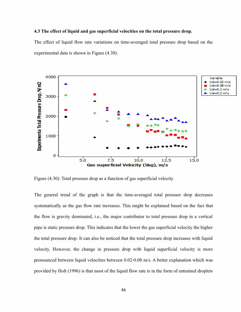
4.3 The effect of liquid and gas superficial velocities on the total pressure drop.
The effect of liquid flow rate variations on time-averaged total pressure drop based on the
experimental data is shown in Figure (4.30).
Figure (4.30): Total pressure drop as a function of gas superficial velocity
The general trend of the graph is that the time-averaged total pressure drop decreases
systematically as the gas flow rate increases. This might be explained based on the fact that
the flow is gravity dominated, i.e., the major contributor to total pressure drop in a vertical
pipe is static pressure drop. This indicates that the lower the gas superficial velocity the higher
the total pressure drop. It can also be noticed that the total pressure drop increases with liquid
velocity. However, the change in pressure drop with liquid superficial velocity is more
pronounced between liquid velocities between 0.02-0.08 m/s. A better explanation which was
provided by Holt (1996) is that most of the liquid flow rate is in the form of entrained droplets
46

and that any further increase in it will only serve to increase the entrained liquid flow rate. As
a result the film flow rate and the film thickness will not change significantly and hence the
limited influence of the liquid flow rate on the two-phase total pressure drop. The effect of the
liquid film fraction on the total pressure drop is depicted in Figure (4.33).
It can be seen that over the range of gas superficial velocities studied, two major regions of
total pressure drop can be identified as a result of gas flow rate variations; the first area being
at low gas velocities between 3.45-9.42m/s, where the total pressure rapidly drops as the gas
superficial velocity increases before the trend is changed to a gradual decrease in the total
pressure drop at higher gas superficial velocities. It is suggested that the change of the slope
linked to a transition of flow regime from churn to annular flow.
It can be concluded therefore that the liquid and gas superficial velocities has a significant
effect on the total pressure drop.
The effect of liquid and gas flow rate on total pressure drop can also be presented by plotting
the total pressure drop as function of mixture superficial velocities (Usg+ Usl) as shown in
Figure (4.41) or gas mass flux (ρg.Usg). Similar forms are reported by researchers, e. g., Kaji et
al (2007), Kaji and Azzopardi (2010), Sawai et al (2004), Holt (1996), and Govan (1990). It is
worth mentioning that in using gas mass flux the effect of gas density is taken into account.
However the differences in the plots for the present work will not change significantly from
what have been discussed earlier and this can be justified based on the fact that Usl << Usg
and ρl remained constant for the data presented. Therefore using mixture velocity or gas mass
flux terms instead of gas superficial velocity will not change the trend of the graph
significantly. However they can remain as a very useful alternative form to present such
experimental data.
47

Figure (4.31): Total pressure drop as a function of mixture superficial velocities.
Figure (4.32): Total pressure drop as a function of gas mass flux (Gg).
48

Figure (4.33): Pressure drop as a function of liquid film fraction.
The total pressure drop is related strongly to the liquid film properties such as the shear stress
on the pipe wall and on the interface between the gas and the liquid phase this is in addition to
the thickness of the film. As can be seen from Figure (4.33), the total pressure drop generally
increases with increasing liquid film fraction but at a liquid superficial velocity of 0.02 m/s,
the total pressure drop was almost constant except for the last value. It can also be observed
that the maximum pressure drop was encountered at the highest liquid superficial velocity.
The reason for this might not be unconnected with the very high liquid density which resulted
in a higher mixture density.
49

4.4 Measured frictional pressure drop.
What is noticeable in Figure (4.40) is that the frictional pressure drop for liquid superficial
velocity of 0.02 m/s is fluctuating between negative and positive values, this was an
unexpected behavior especially for high gas superficial velocities. At such condition, the
liquid film is expected to become unidirectional and flow upward on the wall of the pipe
according to the typical definition of annular flow in vertical pipe by researchers, e.g.,
Azzopardi (2006), and Hewitt and Taylor (1970).
The Kutateladze number (Kug) which is given by equation (4.41).
The average Kutateladze number for liquid superficial velocity of 0.02 m/s and gas superficial
velocity from 6.17 m/s to 16.05 m/s is 4.615. This is greater than the usually quoted transition
value of 3.1 and accordingly the annular flow pattern was expected.
50

Figure (4.40): Measured frictional pressure drop as a function of gas superficial velocity.
However the behavior of frictional pressure drop mentioned above and illustrated in Figure
(4.40), lead to an alternative explanation that the direction of the flow still changing. That is,
the flow pattern is affected by the diameter of the pipe. Therefore, the Kutateladze number
might not be suitable to indicate the churn-annular transition in such diameter pipe, as it does
not contain pipe diameter.
4.5 sensitivity analysis on the effect of diameter on the frictional pressure drop
As stated earlier almost all the available empirical correlations and mechanistic models were
developed with small diameter pipes due to lack of data on large diameter pipes. This is a
major limitation to the universality of its usage to predicting multi-phase pressure drop.
Another limitation is the range of data and the conditions at which these correlations were
developed. The frictional pressure drop from the experiment data used in this work were
under-predicted by all the models. The reason is not farfetched. The range of data at which the
correlations used in this work were developed falls between 1” to 1.5”, which 3.33 to 5 times
less than the diameter used in carrying out the experiment for this work (5” or 0.127 m). This
analysis were carried out for gas velocity of 0.02 m/s and liquid velocity from 6.17 m/s to
16.05 m/s.
Figures (4.80) through to Figure (4.85) show clearly the effect of pipe diameter on the
frictional pressure drop. Pipe diameters of 0.127 m (5”- experimental condition), 0.1016 (4”),
0.0762 (3”) and 0.0381 m (1.5”) were chosen to carry out this sensitivity analysis.
51
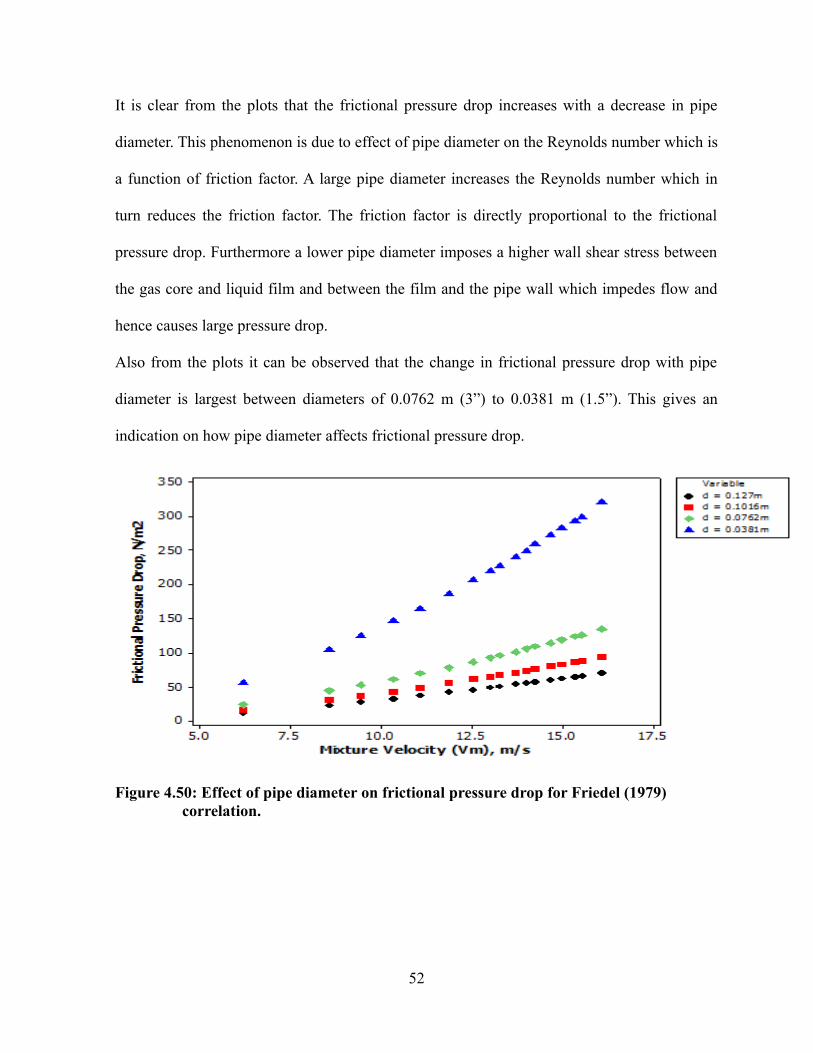
It is clear from the plots that the frictional pressure drop increases with a decrease in pipe
diameter. This phenomenon is due to effect of pipe diameter on the Reynolds number which is
a function of friction factor. A large pipe diameter increases the Reynolds number which in
turn reduces the friction factor. The friction factor is directly proportional to the frictional
pressure drop. Furthermore a lower pipe diameter imposes a higher wall shear stress between
the gas core and liquid film and between the film and the pipe wall which impedes flow and
hence causes large pressure drop.
Also from the plots it can be observed that the change in frictional pressure drop with pipe
diameter is largest between diameters of 0.0762 m (3”) to 0.0381 m (1.5”). This gives an
indication on how pipe diameter affects frictional pressure drop.
Figure 4.50: Effect of pipe diameter on frictional pressure drop for Friedel (1979) correlation.
52
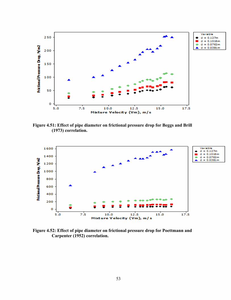
Figure 4.51: Effect of pipe diameter on frictional pressure drop for Beggs and Brill (1973) correlation.
Figure 4.52: Effect of pipe diameter on frictional pressure drop for Poettmann and Carpenter (1952) correlation.
53

Figure 4.53: Effect of pipe diameter on frictional pressure drop for Chisholm (1973)
correlation.
Figure 4.54: Effect of pipe diameter on frictional pressure drop for Modified Hagedorn and Brown (1964) correlation.
54

Figure 4.55: Effect of pipe diameter on frictional pressure drop for Baxendel and Thomas (1961) correlation.
From the above analysis, it can be concluded that the empirical correlations used in this work
are not good enough to predict frictional pressure drop in a large diameter pipe used in this
work. Lists of the known works on the topic can be found in the literature, e. g., Spedding et
al (1998), Kaji and Azzopardi (2010), who reported a noticeable effect of pipe diameter on
two-phase pressure drop in the range of small diameter pipes, i.e., up to 50 mm. This being
the case comparison between present work and the data from different sources in literature
and for different diameter pipes can provide very useful information on the flow behavior as
the effect of such diameter pipes.
55

4.6 Comparison between measured and calculated frictional pressure drop.
There are two components of total pressure drop in vertical multi-phase flow, namely the
frictional pressure drop and the hydrostatic pressure drop. The hydrostatic component of the
experimental pressure drop was calculated using the mixture densities of the experimental
fluids (air and water). The calculated hydrostatic pressure drop was subtracted from the total
pressure drop to obtain the frictional pressure drop.
There is an unsavory trend in the frictional pressure drop of the experimental data. The values
of the experimental frictional pressure drop is decreasing with an increase in void fraction (or
decrease in film fraction). This is a highly unexpected behavior because as flow evolves along
the flow string gas increasingly occupies the pipe area more than the liquid thereby
contributing more to the shear stress and hence frictional drop.
There is an explanation to this unexpected behavior. It could certainly be that most of the
liquid film fraction is over-estimated. This is as a result of an assumption in the experimental
data that the sum of the void fraction and liquid film fraction is equal to unity. During annular
flow regime this assumption can lead to a considerable error in pressure drop prediction. The
entrainment of this liquid fraction increase as the gas and liquid superficial velocity increases.
This is because a portion of the liquid is entrained as droplets in the central gas core due to
turbulence. This liquid fraction does not contribute to the frictional pressure drop. This lead to
an under-estimation of the frictional pressure drop and the degree of under-estimation
increases as flow evolves. This made the experimental frictional drop and the calculated ones
incompatible for an effective comparison, though the values of the calculated frictional
pressure drops falls short of the measured values regardless.
56

4.7 Comparison of experimental total pressure drop with results from empirical correlations.
Several empirical correlations on two-phase gas and liquid flow was investigated to check
their performance and validity in characterizing frictional, and hence total pressure drop for
the conditions studied in this work (for large diameter air-water flow in a vertical pipe). There
has been little experimental data on multi-phase pressure drop in vertical pipe, hence there is
no known correlation on this subject on large diameter pipes (>100 mm). The empirical
correlations in literature are mainly based on small diameter pipes and this puts a limitation on
their usage to characterize multi-phase flow in pipes diameters in the range of those
commonly used in the oil and gas industry.
The motive of this work is to compare the pressure drop derived from those empirical
correlations to the actual pressure drop from experimental study. This would give us an idea
on how each of these empirical correlations perform as compared to the actual results, and
more importantly it would give us an information on the effect of pipe diameter on the
pressure drop.
The correlations chosen for this study include; Friedel et al (1979), Beggs and Brill (1973),
Poettmann and Carpenter (1952), Chisholm (1973), Modified Hagedorn and Brown (1964)
and then Baxendel and Thomas (1961) correlations. Each of these correlations were used to
calculate the pressure drop using the same set of data derived from the experimental study.
The calculation steps and excel model are provided in appendix A.
Table (4.1) show the results of the pressure drop of selected empirical correlations against the
results of the pressure drops calculated from six different empirical correlations. The pressure
57

drop values were derived from a liquid superficial velocity of 0.02 m/s and gas superficial
velocity ranging from 6.17 m/s to 16.05 m/s.
Table (4.1): Comparison of calculated total pressure drop with experimental results.
4.71 Cross plot comparison
Cross plots were used to compare the performance of all the selected models. A 45° straight
line between the calculated pressure drop values versus measured pressure drop values is
plotted which represents a perfect correlation line. When the values go closer to the line, it
indicates better agreement between the measured and the estimated values. When the values
are well above or below the 45° line, it indicates over-prediction and under-prediction
respectively
58

Figure (4.711): Cross plot of pressure drop for all the selected correlations.
Figure (4.711) present cross-plots of estimated pressure drop versus measured pressure drop
for all the investigated methods. It has been noticed that all the six methods presented over-
estimated the pressure drop by some degree but some are closer to experimental value than
others.
The common obstacle for using a pressure drop method whether it is an empirical correlation,
a mechanistic model or an artificial neural network model is that most of these models are
applicable for specific range of data and conditions in order to predict the pressured drop
accurately. However, in some cases, it can work well also in some actual filed data with
acceptable prediction error. (Musaab and Mohammed, 2007)
59

To analyze and compare the effectiveness of each correlation or model, the values of both
measured and predicted pressure drop are recorded. All the selected correlations and models
are evaluated using actual filed data where the predicted pressure drop is compared to the
measured one.
It is worthy to mention that there are still many empirical correlations and mechanistic models
in the literature which have not been evaluated in this study and may have more or less
accurate results when predicting pressure drop in vertical wells. However, the methods were
selected based on the authors’ perspective. Therefore, all the conclusions and
recommendations were based on the selected methods.
60

4.8 Regression analysis using minitab-16 statistical software
Figure (4.81): Regression analysis of experimental and calculated results.
61

Cubic regression was chosen as against linear or quadratic regression because it better
captures the relationship between the experimental results and that of the various empirical
correlations.
Figure 4.82 depicts side by side the closeness or otherwise of the results of the various
empirical correlation to the experimental results.
Figure (4.82): Diagnostic report of measured and calculated results.
62

From Figure (4.96) it can be seen that the results from the empirical correlations follows a
similar trend to the experimental total pressure drop results. All the correlations slightly over-
predict the total pressure drop with the results of Chisholm (1973) having the highest over-
prediction with a mean pressure drop of 621.11 N/m2 as compared to the mean pressure drop
of 550.23 N/m2 for the experimental result. The modified Hagedorn and Brown (1964) came
closest to the experimental result with a mean pressure drop of 564.47 N/m2. This can be seen
more clearly in Figure (4.97).
Table (4.2): Descriptive statistics report of measured and calculated results.
Figure (4.84) mirrors the comparison of the experimental result as against the results of the
six empirical correlations chosen for this work. All the correlations followed the same trend as
the experimental results.
63
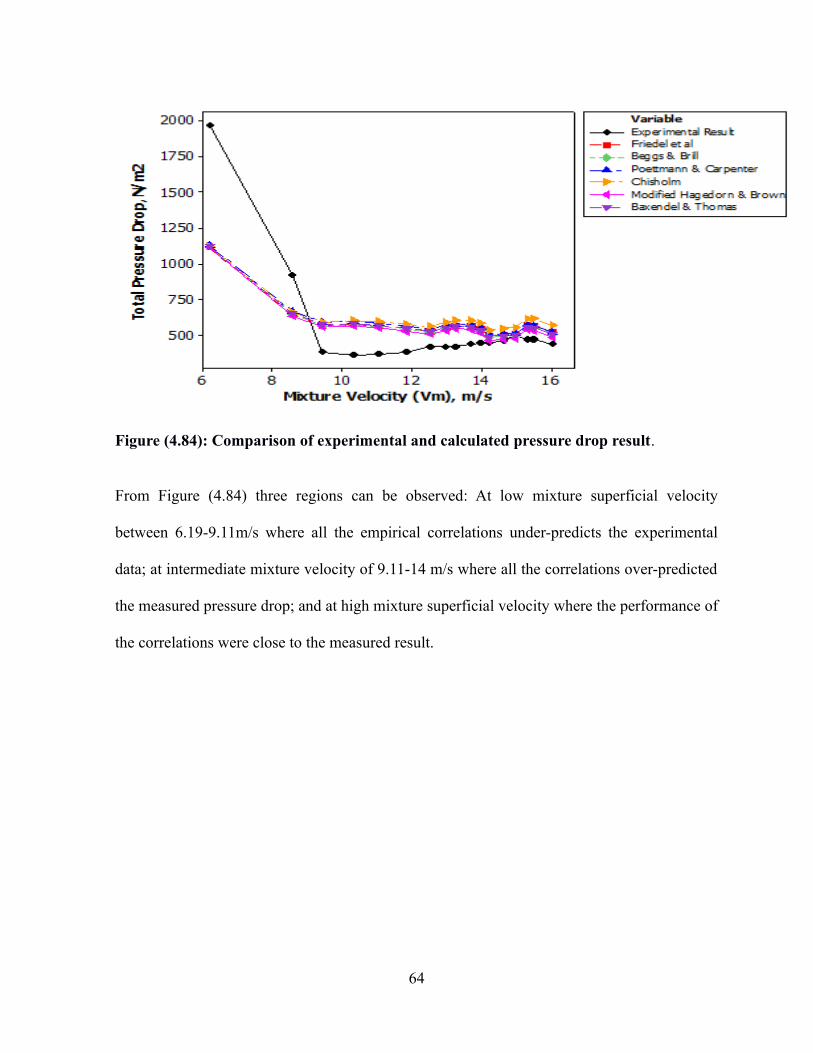
Figure (4.84): Comparison of experimental and calculated pressure drop result.
From Figure (4.84) three regions can be observed: At low mixture superficial velocity
between 6.19-9.11m/s where all the empirical correlations under-predicts the experimental
data; at intermediate mixture velocity of 9.11-14 m/s where all the correlations over-predicted
the measured pressure drop; and at high mixture superficial velocity where the performance of
the correlations were close to the measured result.
64

CHAPTER FIVE
CONCLUSION/RECOMMENDATION/FUTURE WORK
5.1 ConclusionThe main points and conclusion to be drawn from this can be summarized as follows:
The effect of gas superficial velocity on the time-averaged pressure drop in the range
of conditions studied in this work can be identified in two distinct regions, namely the
lower gas superficial velocity region and the upper gas superficial velocity region. In
the lower region between 3.45 m/s to 7 m/s the time-averaged pressure drop decreases
sharply with an increase in gas superficial velocity whilst at higher gas superficial
velocities the decrease is more gradual. On the other hand, the time-averaged pressure
drop increases with an increase in liquid superficial velocity.
The total pressure drop profile becomes less erratic (approaches a constant value) with
time along the pipe length as the gas superficial velocity increases at constant liquid
superficial velocity. In other words, the extent of fluctuation in the pressure drop
grows as the gas flow-rates are reduced.
There is a considerable effect of pipe diameter on frictional pressure drop. From the
sensitivity analysis carried out, it can be noticed that the effect of pipe diameter on
frictional pressure drop is more pronounced at a low diameter range between 0.0762
mm (3”) and 0.0381 mm (1”) especially for Poettmann and Carpenter (1952)
correlation where the sensitivity is quite large. Hence diameter consideration should
play an important role in flow design and optimization.
Total pressure drop increases with an increase in liquid film fraction.
65

The measured total pressure drop and the calculated total pressure drop follow the
same trend. But all the six empirical correlations selected slightly over-predicted the
total pressure drop. The modified Hagedorn and Brown (1964) correlation came
closest to the experimental result while the largest over-prediction was observed with
Chisholm (1973) correlation.
5.2 RecommendationFrom the analysis carried out and the conclusion thereof, the modified Hagedorn and Brown
(1964) is recommended to predict two-phase vertical pressure drop in the absence of an
experimental work.
5.3 Future workThere are still a lot of work to be done in this complex area of research especially in large
diameter pipes. From the results of this work the following areas of research for further work
are recommended:
Extend this work using fluids closer in terms of physical properties to those used in the
oil and gas industry.
Employing wider range of gas and liquid velocities in order to model exactly what
happens in annular flow.
66

REFERENCE
Mohammed Zangana, (2011), “Film Behavior of Vertical Gas-Liquid Flow in a Large
Diameter Pipe”. Department of Chemical and Environmental Engineering, University of
Nottingham, UK.
M.Zangana, G.P. Van der Meulen and B.J.Azzopardi (2010), “The Effect of Gas and
Liquid Velocities on Frictional Pressure Drop in Two Phase Flow for Large Diameter Vertical
Pipe”. Process and Environmental Engineering Research Division, Faculty of Engineering,
University of Nottingham, UK.
Gabor Takacs, (2001), “Considerations on the Selection of an Optimum Vertical Multiphase
Pressure Drop Prediction Model for Oil Wells”. University of Miskolc, Hungary.
Mars Khasanov, Rinat Khabibullin, Vitaly Krasnov, Alexander Pashali, and Slava Guk,
(2007), “A Simple Mechanistic Model for Void Fraction and Pressure Gradient Prediction in
Vertical and Inclined Gas/Liquid Flow”. Rosneft Oil Company.
Poettmann and Carpenter (1952), “The Multi-phase Flow of Gas, Oil, and Water through
Vertical Flow String with Application to the Design of Gas-lift Installations” Philips
Company, Okla.
James P. Brill (University of Tulsa) and Hemanta Mukherjee (Shlumberger Oilfields,
West and South Africa), (1999), “Multi-phase Flow in Wells”
G.J. Zabaras (1994), “Physical Modelling of Vertical Multiphase Flow Prediction of
Pressure Gradients in Oil and Gas Wells” Shell Development Co. Texas, USA.
Khalid Aziz (University of Calgary, Alberta), George W. Govier (Alberta Energy Resources
Conservation Board), Maria Fogarasi (University of Calgary Alberta), “Pressure Drop in
Wells Producing Oil and Gas” (1972), Calgary Alberta.
67

George H. Fancher, Jr. and Kermit E. Brown (1963) “Prediction of Pressure Gradients for
Multiphase Flow in Tubing” University of Texas, USA.
Alton R. Hagedorn and Kermit E. Brown (1965) “Experimental Study of Pressure
Gradients Occurring During Continuous Two-Phase Flow in Small-Diameter Vertical
Conduits”. University of Texas, USA.
G. L. Chienci, G. M. Ciucci, and G. Sclocchi (1974), “Two-Phase Vertical Flow in Oil
Wells– Prediction of Pressure Drop”, AGIP Exploration & Production.
Peter Griffith, Chun Woon Lau, Pou Cheong Hon, and John F. Pearson, (1973),” Two
Phase Pressure Drop in Inclined and Vertical Oil Wells”, Department of Mechanical
Engineering, M.I.T. ,Cambridge, Mass., U.S.A.
K.M. Reinicke, R. J. Remer and G. Hueni, (1987) “Comparison of Measured and Predicted
Pressure Drops in Tubing for High-Water-Cut Gas Wells”, SPE Production Engineering.
A. Rashid Hasan, (SPE, U. of North Dakota), C. Shah Kabir, (SPE, Schlumberger Overseas
S.A), (1988), “A Study of Multiphase Flow Behavior in Vertical Wells”
R.I. Issa and Z.F. Tang, (1991) “Prediction of Pressure Drop and Hold-Up in Gas/Liquid
Flow in Pipes Using the Two-Fluid Model”. Mineral Resources Engineering, Imperial
College, London, U.K.
J.K. Pucknell, J.N.E. Mason, and E.G. Vervest (1993) “An Evaluation of Recent
Mechanistic Models of Multiphase Flow for Predicting Pressure Drops in Oil and Gas Wells”.
BP Exploration.
Musaab M. Ahmed and Mohammed A. Ayoub, (2004), “A Comprehensive Study on the
Current Pressure Drop Calculation in Multiphase Vertical Wells; Current Trends and Future
68

Prospective”, Petroleum Engineering Department, Faculty of Geosciences and Petroleum
Engineering, Universiti Teknologi PETRONAS, Bandar Seri Iskandar, Malaysia.
G. J. Zabaras, “Physical Modelling of Vertical Multi-phase Flow: Prediction of Pressure
Gradients in Oil and Gas Wells”. Shell Development Company.
Kaji, R., Omebere-Iyari, N. K., Hernandez-Perez, V., and Azzopardi, B. J., (2007), "The
Effect of Pipe Diameter on Flow Pattern in Vertical Up-flow", 6th Int. Conf Multiphase Flow,
Leipzig, Germany.
Two Phase Flow Regimes in Reduced Gravity, NASA Lewis Research Center Motion Picture
Directory 1704. By J. B. McQuillen, R. Vernon and A. E. Dukler.
www3.nd.edu/~mjm/flow.regimes.html
69

NOMENCLATURE
Symbol Description UnitA Cross sectional area m2
D, d, do Diameter of pipe mdL, dz Change in length mΔPf Frictional Pressure drop N/ m2
f/fn Friction factor/ two phase friction factor Dimensionlessg Gravitational acceleration m/sKug Kutateladze number DimensionlessNRe Reynolds Number Dimensionlessp Pressure N/m2
qg Gas flow rate m3/sqL Liquid flow rate m3/sGL Liquid mass flux Kg/ m2sGG Gas mass flux Kg/ m2s UM ,Vm Mixture superficial velocity m/sUSG , Vsg Gas superficial velocity m/sUSL , Vsl Liquid superficial velocity m/sx Liquid quality, dimensionlessM Mass flow rate Kg/sE,F,H,Fr, and We Friedel’s factors dimensionless/ Фch Friedel’s/Chisholm’s two-phase multiplier dimensionless
R/r Pipe radius m
Nd, NL, NLV, and Ngv Duns and Ros dimensionless group
GREEK SYMBOLS
λL Liquid film fraction, dimensionlessε Gas void fraction dimensionless
70

µg Gas viscosity cPµ, µL Liquid viscosity Kg/m.sµm Mixture viscosity Kg/m.s
ρl Liquid density Kg/m3
ρg Gas density Kg/m3
ρm ,ρn Density of the gas-liquid mixture Kg/m3
σ Surface tension N/m
ᵠ Factor to correct film fraction for
pipe inclination
Dimensionless
C Beggs and Brill dimensionless
parameterτ Wall shear stress N/m2
71

SUBSCRIPTS/SUPERSCRIPTS
H
Hydrostatic
f, Fr
Frictional
a,b, and c
Correlations for horizontal liquid
holdup
e,f,g, and h
Correlation for C
Lo Liquid
only/Liquid phase
Go Gas
only/Gas phase
G, g Gas phase
72

73

APPENDIX A
CALCULATION PROCEDURES FOR SELECTED MODELS
Friedel Correlation:
The correlation method for Friedel (1979) utilizes a two-phase multiplier. The following steps
were used in estimating the frictional pressure drop through Friedel correlation:
The dimensionless factors, We Fr, E, F and H are as follows:
Friedel’s two-phase multiplier is:
Chisholm Correlation:
Chisholm’s parameter B = 4.8 for mas flux G< 500 kg/m2s
For Re > 2000
Chisholm’s two-phase multiplier is calculated as:
Where n is the exponent from the frictional factor expression of Blasius (n = 0.25)
Beggs and Brill correlation:
The first step to calculating the pressure drop due to friction is to calculate the empirical parameter S. The value of S is governed by the following conditions:
Where are correlation constants for horizontal liquid hold-up (a, b and c are respectively
0.845, 0.5351 and 0.0173)
The factor to correct λL for the effect of pipe inclination is given by
Where e, f, g and h are correlations for C. The values of e, f, g and h are respectively 0.011,
-3.768, 3.539 and -1.614.
since y < 1
Where is the normalizing friction factor which is derived from Drew et al equation given by
And f is the two phase friction factor
74

Modified Hagedorn and Brown
Equations for Duns and Ros dimensionless group
The pipe is assumed hydraulically smooth and the frictional factor is given by
Poettmann and Carpenter and Baxendel and Thomas
The values of were calculated and the following graph of frictional factor against was
digitized used a digitizing software and the values of the corresponding frictional factor for
every was derived.
75

Figure A1: Friction factor chat for different empirical correlations.
APPENDIX B
76
Table B1: Fluid and Pipe geometric properties.

77

78

79

80

81

82


![Cyclone - Progepi · b. Cyclone diameter [from 0.01 to 3 m] c. Cut diameter [from 0.2 to 20 μm] d. Cyclone efficiency [from 0 to 100%] e. Pressure drop [from 10 to 1 000 Pa] - Cyclone](https://img.dokumen.tips/doc/110x75/5f557a33485e9871c8370958/cyclone-progepi-b-cyclone-diameter-from-001-to-3-m-c-cut-diameter-from-02.jpg)