Embed Size (px)
Citation preview


DESTRUCTION NOTICE
FOR CLASSIFIED DOCUMENTS, FOLLOW THE PROCEDURES IN DoD 5200.22-M, INDUSTRIAL SECURITY MANUAL, SECTION 11-19 OR DoD 5200.1-R, INFORMATION SECURITY PROGRAM REGULATION, CHAPTER IX. FOR UNCLASSIFIED, LIMITED DOCUMENTS, DESTROY BY ANY METHOD THAT WILL PREVENT DISCLOSURE OF CONTENTS OR RECONSTRUCTION OF THE DOCUMENT. DISCLAIMER THE FINDINGS IN THIS REPORT ARE NOT TO BE CONSTRUED AS AN OFFICIAL DEPARTMENT OF THE ARMY POSITION UNLESS SO DESIGNATED BY OTHER AUTHORIZED DOCUMENTS. TRADE NAMES USE OF TRADE NAMES OR MANUFACTURERS IN THIS REPORT DOES NOT CONSTITUTE AN OFFICIAL ENDORSEMENT OR APPROVAL OF THE USE OF SUCH COMMERCIAL HARDWARE OR SOFTWARE.

i
REPORT DOCUMENTATION PAGE Form Approved OMB No. 074-0188
Public reporting burden for this collection of information is estimated to average 1 hour per response, including the time for reviewing instructions, searching existing data sources, gathering and maintaining the data needed, and completing and reviewing this collection of information. Send comments regarding this burden estimate or any other aspect of this collection of information, including suggestions for reducing this burden to Washington Headquarters Services, Directorate for Information Operations and Reports, 1215 Jefferson Davis Highway, Suite 1204, Arlington, VA 22202-4302, and to the Office of Management and Budget, Paperwork Reduction Project (0704-0188), Washington, DC 20503
1.AGENCY USE ONLY
2. REPORT DATE August 2007
3. REPORT TYPE AND DATES COVERED Final
4. TITLE AND SUBTITLE Mini-Rocket User Guide
5. FUNDING NUMBERS
6. AUTHOR(S)
George A. Sanders, III and Ray Sells
7. PERFORMING ORGANIZATION NAME(S) AND ADDRESS(ES)
8. PERFORMING ORGANIZATION REPORT NUMBER
TR-AMR-SS-07-27
9. SPONSORING / MONITORING AGENCY NAME(S) AND ADDRESS(ES) 10. SPONSORING / MONITORING AGENCY REPORT NUMBER
11. SUPPLEMENTARY NOTES 12a. DISTRIBUTION / AVAILABILITY STATEMENT
Approved for public release; distribution is unlimited. 12b. DISTRIBUTION CODE A
13. ABSTRACT (Maximum 200 Words) This document describes the use of a missile/rocket fly-out model that represents a significant advance in efficiency for these type of simulations given its modest requirements for complexity and runtime efficiency. The model is useful for generating trajectories and associated flight parameters for multi-stage powered missiles flying over a rotating, spherical earth. The model uses a unique osculating plane formulation that preserves relatively high fidelity while maintaining run-time efficiency and simplicity of input. This formulation provides for user-specified flight guidance options including ballistic flight and profiles for acceleration, flight path angle rate, and flight path angle. This model was designed to expedite many of the same analyses conducted with the old industry-standard ROCKET code – hence the name “Mini-Rocket.” See page ii 14. SUBJECT TERMS
15. NUMBER OF PAGES 70
16. PRICE CODE
17. SECURITY CLASSIFICATION OF REPORT
UNCLASSIFIED
18. SECURITY CLASSIFICATION OF THIS PAGE
UNCLASSIFIED
19. SECURITY CLASSIFICATION OF ABSTRACT
UNCLASSIFIED
20. LIMITATION OF ABSTRACT
SAR NSN 7540-01-280-5500 Standard Form 298 (Rev. 2-89)
Prescribed by ANSI Std. Z39-18 298-102
Commander, U.S. Army Research, Development, and Engineering Command ATTN: AMSRD-AMR-SS-AE Redstone Arsenal, AL 35898
C++, Object-Oriented, Missile Simulation, 6 Degree-of-Freedom, Mini-Rocket

ii
ABSTRACT (CONTINUED
While this manual documents the use of a standalone, executable version of Mini-Rocket, it also provides enough information to configure the Mini-Rocket source code as an embedded model and/or to modify it for a specific application.
Mini-Rocket was built with C++ Model Developer (CMD). CMD is a highly-refined C++ source code environment for building missile simulations such as this one. CMD provides a common platform for building a wide range of missile simulations ranging from simple fly-out models to high-fidelity six Degree-of-Freedom (DOF) simulations. The benefit is a clearly structured architecture that makes it easy to maintain and discern model source code. However, no C++ knowledge is needed to use Mini-Rocket.

Mini-Rocket User Guide
iii
EXECUTIVE SUMMARY
Mini-Rocket is a very easy-to-configure, multiple Degree-of-Freedom (DOF) missile and rocket fly-out model that accurately generates trajectories in three-dimensional space, including maneuver characteristics. It features an advanced algorithm that accurately models missile dynamics at a fraction of the computational cost of conventional 6-DOF simulations while maintaining a significant amount of the fidelity. The program is ideal for those analyses requiring trajectory modeling without the necessity of detailed modeling of the onboard missile subsystems.
Program features include quick generation of trajectories and associated flight parameters for multi-staged rockets and missiles flying over a spherical, rotating earth. In addition to simple ballistic flight, user-selectable guidance options include user-specified profiles for acceleration, flight path angle rate, and flight path angle.
For maximum flexibility, the program is configured as a simple console application that retrieves data from an input data file at runtime. The program is written in standard C++ so that it can be readily compiled and ran on a wide range of computer operating systems. Mini-Rocket provides a viable alternative to 6-DOF simulation for many cases where 3-DOF simulation is inadequate and represents a significant advance in utility for these type of simulations given its modest requirements for complexity and runtime efficiency.

Mini-Rocket User Guide
iv
PREFACE
The Advanced Experimentation Branch of the System Simulation and Development Directorate (SSDD-AE), Aviation and Missile Research, Development, and Engineering Center (AMRDEC) has as one of its missions the task of developing and/or discovering resources that specifically aid the simulation design and analysis process. The technology initiative that is primarily responsible for this effort is the Aviation and Missile Collaborative Design Environment (AMCODE). The AMCODE is a toolbox that contains resources specifically tailored to optimize the work flow process associated with the digital simulation task. One of the cornerstone resources in the AMCODE tool box is the Mini-Rocket simulation. This tool is uniquely suited for a majority of simulation tasks performed by the SSDD and other AMRDEC directorates. It can be easily coupled with other AMCODE resources, such as a genetic algorithm, to provide powerful and fast turnaround analyses of Army systems. The Mini-Rocket simulation has evolved over the past 20 years and, as this report shows, has been extensively proven effective and accurate by numerous users on a wide variety of missile and rocket programs. The Mini-Rocket is a logical choice for AMCODE. It currently supports the design trade studies for Advanced Technology Objective (ATO) programs within the AMRDEC and other Army labs. It is also the backbone architecture for effectors (guns, missiles, lasers) in the AMRDEC Missile Server Executable Code (ICD Version 2.3).
George A. Sanders, III
“Don’t put another ‘six-dof’ into our ‘six-dof’,” our lead simulationist said (or really commanded) as I was given instructions to upgrade the target model in our interceptor missile 6 Degree-of-Freedom (6-DOF) simulation. The modeling requirement was somewhat unique: we needed to model the sudden in-and-out-of-plane, “jinking” motion of a postulated maneuvering re-entry vehicle. This new target was beyond the capability of the existing point-mass target model (3-DOF) that heretofore had served us well. On the other hand, the complexity of upgrading the model to a full 6-DOF representation was clearly overkill given the fidelity required for this target. The timeframe was 1985. Little did I know at the time that my response to this model requirement would begin an over 20-year model legacy whose wide range of application I could then never have imagined.
A simple, but powerful, equations-of-motion formulation was arrived at after seemingly endless trials and explorations into the arcane aspects of rigid body dynamics modeling. The search ended with the discovery of a unique way to apply an osculating plane to describe the motion. This resulted in a computationally efficient, intuitive algorithm that was first mechanized in a FORTRAN subroutine. It allowed the modeling of a wide variety of trajectory motions in three-dimensional space, but at much less the cost and complexity of a full 6-DOF representation. The subroutine quickly proved itself capable of simulating a wide variety of target trajectory behaviors for objects flying in the atmosphere. But was the model only confined to unpowered flight trajectories? What if a longitudinal force was added to emulate an axial thrust component?
With the addition of an axial force, the subroutine rapidly evolved into a standalone rocket and missile model where the trajectory could begin from a stationary launch point. This efficient trajectory generator quickly found application for a number of modeling tasks. Depending on analysis needs and the advance of programming language maturity (mine as well as advance in state-of-the-art), it was coded in many dialects of Basic, Pascal, C, Ada, and many others. It was

Mini-Rocket User Guide
v
used by myself and a growing list of users from things as simple as the motion of a piece of debris, to endo- and exo- interceptor missiles, to intercontinental ballistic missiles, to theater and tactical missiles and targets, and even to ground-test, sled-launched test articles. Versions of the model were also coded to be embedded as missile model representations in larger battlefield simulations1. There are doubtless many other applications that I am unaware of. Every now-and-then, someone unexpectedly informs me that they are using the model or they have seen it used (in many cases, they had no indication of the origin but saw my name in the source code!). The model representations have proved their worthiness by providing efficient analysis results in the many cases where the overhead and resources of a full-up 6-DOF were not required. Over time, the domain for requiring trajectory modeling above that of a 3-DOF but not needing those of a 6-DOF proved to be vast and the model fit. It fit very well.
Its widening use dictated that it be called something, so the name Mini-Rocket was adopted and seemed to “stick.” Many users had previously used the industry-standard ROCKET2 code that was very capable, but had become somewhat antiquated by the advance of programming language technology. “Mini” implied that tools developed from the algorithms had much of the functionality of ROCKET but that the code was more streamlined and easier to use. Using “ROCKET” in the name conveyed functionality to a community that was already aware of the very successful legacy of ROCKET (but recognizing that Mini-Rocket was developed completely independently from ROCKET).
The formulation and publication of the C++ Model Developer3 (CMD) provided an ideal medium for a formalized mechanization of the Mini-Rocket model. CMD was expressly designed for building simulations of dynamical systems and has a well-defined and mature architecture. CMD’s concise architecture was a natural complement for the simple but powerful algorithms in the Mini-Rocket equations of motion. The CMD-implementation of Mini-Rocket continues and expands on the successful original Mini-Rocket legacy of a powerful tool for trajectory analysis. The CMD-based Mini-Rocket is currently being used for a wide variety of missile modeling applications by a diverse community within the U.S. Army’s AMRDEC and elsewhere.
What began as a FORTRAN subroutine has grown into a versatile and widely-used tool for trajectory modeling and will certainly continue to proliferate. The malleability and simplicity of the algorithms makes it easily tailorable for many applications. This guide aims to continue and encourage this proliferation by undergirding the tool with formalized implementation and documentation.
Ray Sells May 24, 2007
1 Extended Air Defense Simulation (EADSIM) Methodology Manual, Section 5.9, “Interceptor Missile Flight.” Teledyne Brown Engineering, Huntsville, AL, 1995. 2 Boehm, Barry W. Rocket: Rand's Omnibus Calculator of the Kinematics of Earth Trajectories. Prentice Hall, (1964). 3 Sells, H.R., Sanders, G.A., Snyder, G., Hester, J.W., and Painter, L. 2005. “C++ Model Developer (CMD) User Guide.” U.S. Army Technical Report AMR-SG-05-12, April 2005.

Mini-Rocket User Guide
vi
TABLE OF CONTENTS
Page
1. INTRODUCTION ................................................................................................... 1
2. INSTALLATION..................................................................................................... 3
3. INPUT DATA FILE ................................................................................................ 4
3.1 Data Formating ................................................................................................... 4 3.2 Scenario and Control Data.................................................................................. 5 3.3 Stage Section Data.............................................................................................. 8
4. MATHEMATICAL DESCRIPTION.................................................................... 15
5. REAL WORLD COMPARISON........................................................................... 25
5.1 Initial Benchmark Comparison for Accuracy (1993).................................... 25
5.2 A Trial of Successful Comparisons ................................................................. 28
5.2.1 Integrated System Test Capability ........................................................... 28 5.2.2 Anti Satellite Mission Scenario Analysis ................................................ 30 5.2.3 EADSIM .................................................................................................. 32
5.3 A Legacy of Successful Comparisons Continues........................................... 32
5.3.1 Extended Air Protection and Survivability Program (EAPS).................. 32 5.3.2 Interactive Distributed Engineering Evaluation and Analysis Simulation (IDEAAS).............................................................................. 35
5.4 Conclusion ......................................................................................................... 37
6. HOW MINI-ROCKET WAS BUILT.................................................................... 38
7. SUMMARY.............................................................................................................. 40
REFERENCES ........................................................................................................ 41
ACRONYMS............................................................................................................ 42
APPENDIX 1 MAKING PLOTS .......................................................................... A-1
1.1 Installing the Plotter ............................................................... A-1 1.2 Basic Usage .............................................................................. A-1 1.3 Scaling ...................................................................................... A-3 1.4 Exporting Plots for Publication ............................................. A-3
APPENDIX 2 EXAMPLE CASE.......................................................................... A-2
Mini-Rocket User Guide
vii
LIST OF ILLUSTRATIONS
Figure Title Page
1. Mini-Rocket Coordinate Frame Definition........................................................... 13
2. Missile Body Coordinate Frame............................................................................. 17
3. Guidance Steering Reference Frame ..................................................................... 19
4. Airframe Response Feedback Loop....................................................................... 20
5. Commanded Acceleration Constraints.................................................................. 21
6. Missile Free-Body Diagram .................................................................................... 21
7. Aries Simulation Comparisons............................................................................... 26
8. ISTC Simulation Comparisons............................................................................... 29
9. STARS Simulation Comparisons ........................................................................... 31
10. EAPS Side-by-Side Simulation Comparisons (6-DOF and Mini Robot)............ 33
11. Ground-to-Ground Missile Simulation Comparison ........................................... 35
12. Prime Contractor Simulation Depiction of Complex “Loop-Back” Maneuver.................................................................................................................. 36
13. Mini-Rocket Replication of “Loop-Back” Maneuver .......................................... 37
14. Object-Oriented Simulation Architecture and Simulation Construction Hierarchy.................................................................................................................. 38
15. OSK Train-of-Objects ............................................................................................. 39

Mini-Rocket User Guide
viii
LIST OF TABLES
Table Title Page
1. Scenario and Control Data Descriptions ............................................................... 6
2. Stage Section Data Descriptions............................................................................. 9

Mini-Rocket User Guide INTRODUCTION
1
1 INTRODUCTION
Mini-Rocket provides the capability to model realistic trajectories associated with the boost and fly-out of a multi-stage missile flying over a rotating, spherical earth. Multi-stage missiles are modeled using flight sections to represent the missile's properties. Each flight section consists of a separate specification for the aerodynamic, propulsion, and guidance parameters. Within a flight section, any combination or sequence of guidance modes can be selected including ballistic, prescribed acceleration, prescribed flight path angle rate or prescribed flight path angle. This flexible combination of guidance options makes it possible to replicate virtually any missile steering behavior, both in-plane and out-of-plane in three-dimensional coordinate space. A unique osculating plane representation keeps prescribed maneuvers clearly discernable in either pure pitch or yaw even though the missile motion itself may be complex.
The flight trajectories during boost and fly-out are realistically constrained with aerodynamic and structural capabilities. Lateral acceleration for steering is aerodynamically limited according to a user-specified angle-of-attack. Also a "hard" limit is placed on lateral steering acceleration representing maximum g-loading structural capabilities.
This missile model was formulated with particular attention to the speed of execution. A unique point-mass model with wind-axes is used to include the variation of drag with angle-of-attack as the missile maneuvers without resorting to the computational burden associated with a full 6 Degree-of-Freedom (DOF) rigid body for the missile. Trajectories generated with this modified point-mass model have been shown to closely match those generated by a very high fidelity 6-DOF simulation (within the resolution of time-history plots).
Mini-Rocket was built with C++ Model Developer (CMD)[1]. CMD is a highly-refined C++ source code environment for building missile simulations such as this one. CMD provides a common platform for building a wide range of missile simulations ranging from simple fly-out models to high-fidelity 6-DOF simulations. The benefit is a clearly structured architecture that makes it easy to maintain and discern model source code. However, no C++ knowledge is needed to use Mini-Rocket.
This manual is organized to equip the user to get Mini-Rocket “up and running” as quickly as possible. Following this objective, the following section describes installation which is easily accomplished since Mini-Rocket runs from a command-line interface. The contents of the input data file are then described in a narrative tied to an example set of input parameters. Although not required for operation, an in-depth mathematical description is then presented to give additional insight into the model and how it can be extended. Perhaps the most important question about any modeling tool is how well it represents what is being simulated. Mini-Rocket has been rigorously compared to other accepted models and has obtained the confidence of a wide variety of users for its ability to accurately model trajectories. A variety of example cases supporting this claim are shown in Section 5. Section 6 gives a brief description of Mini-Rocket’s implementation in code using the aforementioned CMD. This section is a starting point for consulting the source code and CMD documentation [1] to understand the code mechanization behind Mini-Rocket. Appendix 1 describes operation of a convenient plotting tool (included with Mini-Rocket) for visualizing output. Appendix 2 builds on the input data

Mini-Rocket User Guide INTRODUCTION
2
description in Section 3 showing a step-by-step example of using Mini-Rocket to generate a trajectory.
While a standalone, executable version of Mini-Rocket is documented in this manual, the underlying code that comprises Mini-Rocket is far more flexible than a simple standalone program. Due to its modular, object-oriented coding structure, the source code is easily configured for a broad range of applications including use as an embedded model in more broadly-scoped simulations or modifications to add additional functionality. Thus, this manual also serves the dual purpose as an introduction and starting point to configure the Mini-Rocket source code for custom-tailored applications.

Mini-Rocket User Guide INSTALLATION
3
2 INSTALLATION
Mini-Rocket is a single executable Windows file that is compatible with any MS Windows machine that has a DOS prompt1. In addition to the single executable file, a data file is also required. Make sure the data file is in the same directory as the executable.
The program is most conveniently executed by typing minirock at the DOS prompt in a console window followed by a file name with the input data.
For example: C:>minirock rocket.dat
If you do not include a file name with the minirock command, you are prompted for a filename:
Mini-Rocket v1.01 by Ray Sells, DESE Research, Inc.
Input file: _
Output is printed directly to the screen after the data file is entered. Normal DOS file commands can be used to redirect output for storage, as needed. Mini-Rocket also automatically pipes data to an output file for post-processing (plotting, for instance). Instructions for this automatic output are in the following section.
1 While the instructions for installing and running Mini-Rocket in this guide are directed at the Windows operating system, installation and running the program will proceed similarly for Unix/Linux operating systems since the program is operated from a command line interface.

Mini-Rocket User Guide INPUT DATA FILE
4
3 INPUT DATA FILE
This section illustrates by example how to configure an input data file to be used by the Mini-Rocket missile fly-out model. The model can be used very effectively by making changes only to the input data file. The input data file specifies the missile's properties, its flight guidance instructions, and data reporting.
The missile fly-out is described by the use of multiple flight sections. Each flight section consists of a separate specification of aerodynamic, propulsion, and mass properties as well as guidance steering commands. Describing the missile as a series of flight sections provides the capability to model virtually any missile. Normally the flight section will correspond to a stage but this does not necessarily have to be the case. The mathematical formulation for each section is identical. Each section consists of specification for
• vacuum thrust profile • specific impulse • nozzle exit area • initial mass • aerodynamic reference area • aerodynamic tables for lift and drag • guidance instructions
Within a section, guidance instructions consist of a table specifying periods of operation (by means of sequentially listed start times) for any combination of four guidance phases:
• ballistic • follow a commanded acceleration profile in the y and z channels • follow a commanded flight path angle rate profile • follow a commanded flight path angle profile
3.1 Data Formatting
Owing to CMD’s input/output system, format restrictions on the input data are very relaxed since all numeric parameters are tagged to an identifier. The only rule on input is that the parameter name must appear followed by its value on a single line. An optional equals sign can be used between the name and value. The data can be specified in any order and there are no spacing or column restrictions on how or where the data can appear. Comments can be freely interspersed throughout the input data file.
Example: The data in the input file can appear as:
tmax = 50. v0 = 100. h0 = 200.

Mini-Rocket User Guide INPUT DATA FILE
5
The model also uses one- and two-dimensional tables in the data file. CMD also provides a very flexible format for specifying tables. The exact format is apparent in the table descriptions that follow.
3.2 Scenario and Control Data
Input data is divided into two sets. The first set (Scenario and Control Data) describes the fly-out scenario and initial conditions as well as execution model options. The second set describes the physical characteristics of each stage including aerodynamics, mass properties, and propulsion. This section describes the first set of data for the scenario and initial conditions.
The following parameters describe the fly-out scenario and model execution instructions.
**** rocket **** tmax = 100. echo = 1 lon0_d = 45. lat0_d = 38.708 v0 = 0.01 h0 = 0.0 az0_d = -70. el0_d = 90.0 xrail=1000.0 nstages = 3 rotating_earth = 1
These parameters are described in Table .
The tag **** rocket **** must appear in the data file before any of the parameters. This provides maximum flexibility to place the parameters anywhere in the file.

Mini-Rocket User Guide INPUT DATA FILE
6
Table 1. Scenario and Control Data Descriptions
Name Description tmax Simulation termination time. Missile launch is at time = 0. The simulation
will also terminate if the missile's altitude is less than zero.
echo echo = 1 to echo contents of data file to screen as they are read. echo = 0 for no printout. It is good practice to echo output while configuring the data file. That way, if the simulation crashes for some reason while reading the input data, you can see the last data item successfully read.
lon0_d Launch point longitude on a spherical earth (deg). lat0_d Launch point latitude on a spherical earth (deg). v0 The velocity of the missile when it is launched relative to the earth's surface
(m/sec). This parameter provides the flexibility of starting the simulation at some time after the missile is actually launched or simulating an object with an initial impulse applied (such as a bullet or an air-launched missile).
h0 Launch point altitude above the spherical earth’s surface (m). az0_d Launch direction azimuth (deg). el0_d Launch elevation (deg). xrail The distance from the launch point over which the missile's gravity turn (or
pitchover) is constrained to zero (m). As its name implies, this parameter can be used to include the effect of a launch rail if the missile is launched non-vertically. The majority of missiles fail to build up enough instantaneous axial acceleration at launch to prevent excessive pitching over (due to gravity) when launched at an angle. Thus a launch rail is used to point the missile immediately after launch, giving it time to accelerate to sufficient velocity to develop lift. This parameter does not necessarily have to correspond to the launch rail's length (if one is used). As an alternative to formulating the guidance commands to make the missile travel a straight line after launch, much larger values of this length can be used (on the order of hundreds of meters or more) to prevent the missile from pitching over due to gravity.
nstages Number of stages. The missile fly-out sequence is divided into discrete stages. Stages are numbered sequentially 1..nstages. Independent properties are specified for each stage. As a special case, two or more stages in this model can be used to describe a single physical stage on the missile whose properties change during flight for some reason. For example, the homing stage may have a protective shroud covering its seeker window in which case its aerodynamic properties would be different for the shrouded versus the unshrouded vehicle. In this case, two stages in this model could be used to describe the two sets of aerodynamic (and mass) properties for this single stage.
rotating_earth A boolean parameter indicating whether or not earth rotation is turned on. rotating_earth = 1 sets the earth rotation rate to 7.292115(10)-5 rad/sec. rotating_earth = 0 sets the earth rotation rate to zero.

Mini-Rocket User Guide INPUT DATA FILE
7
The following parameters specify output instructions to a data file and the screen.
Output fname = OutputRun0.dat pt = 0.01 pt_console = 1.0
These parameters are provided to designate output to the screen and to the output file designated with fname. The tag Output must precede these parameters and designates where in the file for the CMD parser to start looking for the parameters. The output data to the screen and file output are identical. pt and pt_console are the output time increments for the output file and console, respectively.
The parameters specified for output are as they appear in the source code with a p_ prefix. 0 or 1 designates whether or not the variable is output (0-no, 1-yes). For convenience, a description of each parameter is included in the input data owing to the flexible nature of the CMD file parser.
p_range = 1 Ground range over spherical earth surfa ce (m). p_h = 1 Altitude above spherical earth (m). p_vel = 1 Velocity (m/sec). p_mach = 0 Mach number. p_q = 0 Dynamic pressure (N/m2). p_p = 0 Local atmospheric pressure (N/m2). p_vs = 0 Local velocity of sound (m/sec). p_rho = 0 Local atmospheric density (kg/m3). p_gamma_d = 1 Flight path angle, with respect to ho rizontal (deg). p_alph = 1 Total angle-of-attack (deg). p_mass = 0 Mass (kg). p_xstage = 0 Identifier for current stage. p_txv = 0 Vacuum thrust (N). p_tx = 0 Delivered thrust (N). p_amax_alph = 0 Max. acceleration at max.-specified angle-of-attack (m/sec2). p_range_slant = 0 Slant range (m). p_ay = 0 y-acceleration, in velocity axex coordinat e system (m/sec2) p_az = 0 z-acceleration, in velocity axex coordinat e system (m/sec2) p_ax = 0 x-acceleration, in velocity axex coordinat e system (m/sec2) p_xmode = 0 Current guidance mode. p_ay_cmd = 0 Commanded y-acceleration (m/sec2). p_az_cmd = 0 Commanded z-acceleration (m/sec2). p_lat_d = 0 Current latitude (deg). p_lon_d = 0 Current longitude (deg). p_azimuth_d = 0 Current azimuth of velocity vector (deg). p_ca = 0 Axial force coefficient. p_cd = 0 Equivalent drag coefficient. p_cna = 0 Linearized normal force coefficient (/deg ). p_cla = 0 Linearized equivalent lift coefficient (/ deg).
These parameters may appear anywhere in the file; they need not be preceded by a tag.
Mini-Rocket User Guide INPUT DATA FILE
8
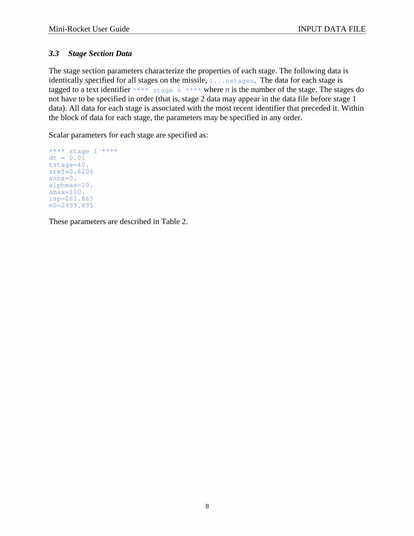
3.3 Stage Section Data
The stage section parameters characterize the properties of each stage. The following data is identically specified for all stages on the missile, 1...nstages . The data for each stage is tagged to a text identifier **** stage n **** where n is the number of the stage. The stages do not have to be specified in order (that is, stage 2 data may appear in the data file before stage 1 data). All data for each stage is associated with the most recent identifier that preceded it. Within the block of data for each stage, the parameters may be specified in any order.
Scalar parameters for each stage are specified as:
**** stage 1 **** dt = 0.01 tstage=40. sref=0.6206 anoz=0. alphmax=20. amax=100. isp=261.865 m0=2499.895
These parameters are described in Table 2.

Mini-Rocket User Guide INPUT DATA FILE
9
Table 2. Stage Section Data Descriptions
Name Description dt Integrating time step (sec). 4th order Runge-Kutta is used for integration.
Note that you can use multiple time steps per stage by simply having two flight sections with identical properties, but with different time steps.
tstage Time to transition to next stage (sec). This time is referenced from the starting time of the current stage (and NOT the current time).
sref Aerodynamic reference area (m2). This parameter is used in conjunction with aerodynamic coefficients to compute lift and drag.
anoz The exit area of the nozzle used for axial propulsion (m2). This exit area is used to adjust the vacuum thrust for atmospheric pressure. The local atmospheric pressure reduces the delivered thrust by the product of the exit area and the local ambient pressure.
alphmax The maximum total allowable angle-of-attack for maneuvering (deg). To enforce realistic aerodynamic maneuvering, the lateral acceleration of a section is limited using the angle-of-attack. The lateral force acting on the vehicle is constrained using the product of the angle-of-attack, the linearized normal force coefficient, the aerodynamic reference area, and the local dynamic pressure. The maximum angle-of-attack for missiles is normally around 20 deg, beyond which the aerodynamics become highly nonlinear and less predictable.
amax An absolute hard limit on how much acceleration the missile can generate for steering (m/sec2). This constraint is intended to reflect the structural limits of the missile. This parameter typically varies 10 - 30 g's for long, slender and short, stubby missiles, respectively. Homing stages or kill vehicles can sometimes tolerate 50 or more g's. The acceleration is also constrained by maximum angle-of-attack depending on the atmospheric regime the missile is operating in.
isp Boost propulsion parameter describing the unit thrust per rate of expenditure of propellant (fuel and oxidizer) (sec) in a vacuum. The thrust per unit rate of propellant expenditure is this parameter multiplied by gravity, g, which yields units of N per kg/sec. This quantity is typically in the range of 250 sec for solid rocket motors at sea level.
m0 The initial mass for each section (kg). Mass is reduced during missile section operation by propellant usage (if any) according to the specific impulse.
Tabular parameters for each stage are specified as follows. The tables can appear in any order; the only caveat is that they should appear after the appropriate stage tag identifier (the CMD parser first finds the stage tag identifier and then looks for the table tag).
The txv_table specifies the axial thrust profile.
txv_table 4 t txv 0.0 119484.02 40.0 119484.02 40.01 0.0 100. 0.0

Mini-Rocket User Guide INPUT DATA FILE
10
This table is the vacuum propulsive thrust acting along the vehicle's longitudinal axis (N). Normally this is the thrust profile during boost. The thrust at any time is linearly interpolated from this table. The delivered thrust is the vacuum thrust minus the product of the nozzle exit area and the local ambient pressure.
The first entry is the table tag which must be txv_table . The number of table entries, 4, follows. The column labels, t and txv , are followed by their entries.
These ca_off and ca_on tables specify the axial-force coefficient data when the axial thrust if off and on, respectively.
ca_off 10 2 amach .2 .9 1.0 1.5 2. 3. 5. 7. 9. 10. alpha 0. 10. ca .223 .223 .415 .409 .466 .460 .369 .383 .304 .307 .233 .261 .188 .214 .177 .201 .177 .200 .178 .200 ca_on 10 2 amach .2 .9 1.0 1.5 2. 3. 5. 7. 9. 10. alpha 0. 10. ca .201 .201 .374 .368 .419 .414 .332 .345 .274 .276 .210 .235 .169 .193 .159 .181 .159 .180 .160 .180 This coefficient is used to calculate the missile's drag along the velocity vector. The drag force is the product of this coefficient converted to wind-axes, the aerodynamic reference area, and the local dynamic pressure. A linear two-dimensional interpolation is used to compute this coefficient as a function of angle-of-attack and Mach number. Two sets of data are provided for the drag coefficient since the drag varies significantly depending on whether the section's axial propulsion is on or off. The exiting plume of the motor's exhaust reduces the drag.
The first entry is the table identifier. The next row of data is the number of Mach # entries and angle-of-attack entries. The specific Mach #’s (rows of data that follow) and angles-of-attack (column of data that follow) are specified as shown. The ca data itself follows.
Mini-Rocket User Guide INPUT DATA FILE
11
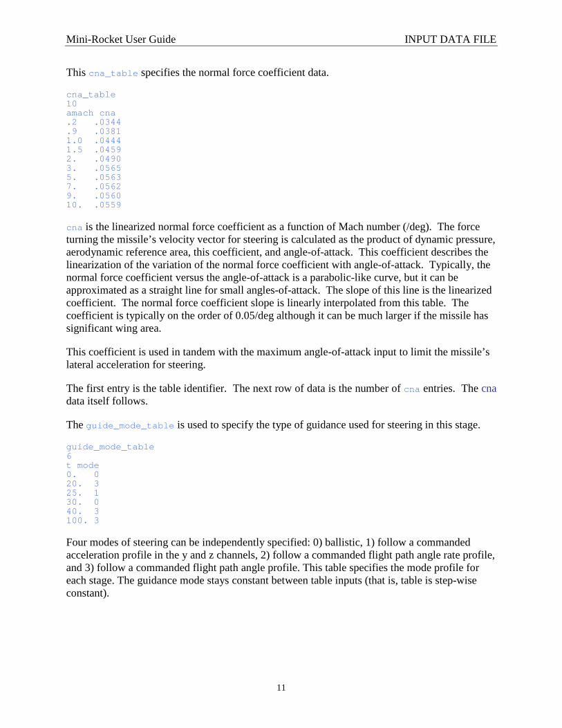
This cna_table specifies the normal force coefficient data.
cna_table 10 amach cna .2 .0344 .9 .0381 1.0 .0444 1.5 .0459 2. .0490 3. .0565 5. .0563 7. .0562 9. .0560 10. .0559
cna is the linearized normal force coefficient as a function of Mach number (/deg). The force turning the missile’s velocity vector for steering is calculated as the product of dynamic pressure, aerodynamic reference area, this coefficient, and angle-of-attack. This coefficient describes the linearization of the variation of the normal force coefficient with angle-of-attack. Typically, the normal force coefficient versus the angle-of-attack is a parabolic-like curve, but it can be approximated as a straight line for small angles-of-attack. The slope of this line is the linearized coefficient. The normal force coefficient slope is linearly interpolated from this table. The coefficient is typically on the order of 0.05/deg although it can be much larger if the missile has significant wing area.
This coefficient is used in tandem with the maximum angle-of-attack input to limit the missile’s lateral acceleration for steering.
The first entry is the table identifier. The next row of data is the number of cna entries. The cna data itself follows.
The guide_mode_table is used to specify the type of guidance used for steering in this stage.
guide_mode_table 6 t mode 0. 0 20. 3 25. 1 30. 0 40. 3 100. 3
Four modes of steering can be independently specified: 0) ballistic, 1) follow a commanded acceleration profile in the y and z channels, 2) follow a commanded flight path angle rate profile, and 3) follow a commanded flight path angle profile. This table specifies the mode profile for each stage. The guidance mode stays constant between table inputs (that is, table is step-wise constant).

Mini-Rocket User Guide INPUT DATA FILE
12
This method of guidance selection provides maximum flexibility in specifying how the missile flies. Any order or sequence of flight modes can be prescribed using a mode or modes more than once, if desired. Note that the commanded flight path mode, when active, always follows the commands in the associated table at that time. Thus only one commanded flight path angle table is needed even though this mode may be specified multiple times at different times in the flight.
Ballistic (mode = 0) is flight with no steering. The forces acting on the missile are only drag, gravity, and axial thrust, if any.
Depending on the flight modes selected, the following tables may be used. They must appear for each stage whether used or not. Linear interpolation is used on all the tables. The last value is used if the current time (independent variable) is greater than the last entry.
The missile can be commanded to follow a pre-specified lateral acceleration steering profile using ay_table and az_table (mode 1).
ay_table 3 t ay 0. 0.0 10. 9.0 40. 9.0 az_table 3 t az 0. -999.0 10. -999.0 100. -999.0 The units are m/sec2. Mini-Rocket uses an osculating plane formulation which greatly simplifies this process. As shown in Figure 1, an orthogonal triad is composed of the missile’s velocity axis (x), an axis perpendicular to the x-axis and tangent to the earth’s surface (y), and a final axis that is the cross-product of the x and y axes (z). Thus the x-z plane is always the pitch plane (up-down) and the x-y plane is the yaw plane (right-left). This makes it very intuitive to prescribe the missile’s motion since +/- z is always up/down and +/- y is always left/right. In other words, the az_table controls pitch and ay_table controls yaw. Contrast this simplicity with having to ascertain what these directions are if a missile body coordinate frame (which rolls) was used to describe the motion.

Mini-Rocket User Guide INPUT DATA FILE
13
tangent toearth's surface
velo
city
vec
tor
position vector
Xbodyv
Ybodyv
Zbodyv
ecix
eciy
eciz
missilepYX
YX
Z
Y
X
bodybody
bodybodybody
relativemissile
relativemissilebody
relative
relativebody
vv
vvv
vp
vpv
v
vv
××
=
××=
=
Figure 1. Mini-Rocket Coordinate Frame Definition

Mini-Rocket User Guide INPUT DATA FILE
14
The missile can be commanded to follow a pre-specified flight path angle rate steering profile in the pitch channel using the gammad_table (mode = 2).
gammad_table 3 t gammad 0. 0.0 10. 0.1 100. 0.1
Units for this table are degree/second. The flight path angle is the angle between the missile's velocity vector and the local earth's surface. In this guidance mode, steering occurs only in the missile's pitch channel; the acceleration to change the heading is zero. Positive gamma_d pitches the missile up.
The missile can be commanded to follow a pre-specified flight path angle steering profile in the pitch channel with the gamma_table (mode = 3).
gamma_table 3 t gamma 0. 0.0 10. 80.0 100. 80.0
Units for this table are degrees. A simple feedback controller is used to command a pitch acceleration based on the difference between the commanded flight path angle and the current flight path angle. The dynamics of this feedback process, along with the gain of the feedback loop, result in a lag corresponding to a first order system with a 1.0 second time constant. In this guidance mode, steering occurs only in the missile's pitch channel; the acceleration to change the heading is zero.
Data for succeeding stages is input in an identical manner. Simply precede the data with ****
stage 2 ****, **** stage 3 ****, and so forth.

Mini-Rocket User Guide MATHEMATICAL DESCRIPTION
15
4 MATHEMATICAL DESCRIPTION
This section describes the mathematical formulation of the missile fly-out model and is intended to give more insight into operation of the program. The following calculations are updated each integrating time step starting at launch. The equations are the same for each stage on a multiple stage missile; stages are defined by specifying different properties for each stage.
The vector magnitude of the missile’s position vector is calculated in Earth-Centered Inertial (ECI) coordinates:
222
ZYX missilemissilemissilemissile pppp ++= (1)
where
=
Z
Y
X
missile
missile
missile
missile
p
p
p
p = missile position vector, ECI
The ECI position vector of the missile’s launch point is calculated by
+++++
=)sin()(
)sin()cos()(
)cos()cos()(
0
00
00
0
0
0
late
elonlate
elonlate
launch
hr
thr
thr
p
θωθθωθθ
(2)
where
launchp = launch point position vector, ECI coordinates
er = earth’s radius, 6371008.7714 m ( mean radius of semi-axes in WGS84 Ellipsoid)
0h = launch point altitude above spherical earth’s surface
0latθ = launch point latitude
0lonθ = launch point longitude
eω = earth’s rotation rate, 7.292115(10)-5 rad/sec
t = elapsed time since missile launch
The earth’s rotation rate can optionally be set to zero.
The component of the missile’s velocity (in the ECI) frame due to the earth’s rotation is calculated as
−=
−−−
=×=0
X
Y
XY
ZX
YZ
missilee
missilee
missileymissilex
missilexmissilez
missilezmissiley
missileearthearth p
p
pp
pp
pp
pv ωω
ωωωωωω
ω (3)

Mini-Rocket User Guide MATHEMATICAL DESCRIPTION
16
where
earthv = local velocity due to earth’s rotation
=
=
ez
y
x
earth
ωωωω
ω 0
0
= earth rotation rate vector, ECI
The missile’s velocity relative to the earth at the current missile’s position is
222
ZYX relativerelativerelativerelative
earthmissilerelative
vvvv
vvv
++=
−= (4)
where
relativev = missile’s velocity relative to earth
missilev = missile’s velocity referenced to fixed ECI coordinates
Unit vectors for a missile “body” coordinate frame are defined in Figure 2.

Mini-Rocket User Guide MATHEMATICAL DESCRIPTION
17
tangent toearth's surface
velo
city
vec
tor
position vector
Xbodyv
Ybodyv
Zbodyv
ecix
eciy
eciz
missilepYX
YX
Z
Y
X
bodybody
bodybodybody
relativemissile
relativemissilebody
relative
relativebody
vv
vvv
vp
vpv
v
vv
××
=
××=
=
Figure 2. Missile Body Coordinate Frame
The cross product relativemissile vp × is 0 for a vertical launch leaving the axis Ybodyv undefined. In
this special case, the launch elevation angle is adjusted to 1 ,2
<<− εεπ so that the cross product
is nonzero.
The flight path angle is calculated
⋅−= −
relativemissile
relativemissile
vp
vp1cos2
πγ (5)
The altitude above the spherical earth’s surface is
emissile rph −= (6)

Mini-Rocket User Guide MATHEMATICAL DESCRIPTION
18
The dynamic pressure and Mach number are
sound
relative
relative
v
vM
vq
=
= 2
2
1 ρ (7)
where
ρ = atmospheric density at current altitude, h
soundv = speed of sound at current altitude, h
A 1962 standard atmosphere model is used to define the atmospheric properties.
The vacuum thrust, vacuumT , is linearly interpolated from a table of vacuumT vs. time.
The delivered thrust, deliveredT , is calculated:
PaTT nozzlevacuumdelivered −= (8)
where
nozzlea = Nozzle exit area
P = atmospheric pressure at current altitude, h
The delivered thrust, deliveredT , is zero if 0 <− PaT nozzlevacuum .
The change in mass with propellant consumption is calculated:
dtI
Tm
sp
vacuum ∫−=& (9)
where
spI = Motor specific impulse
Guidance steering is accomplished by defining components of lateral acceleration along the body y and z axes as shown in Figure 3.

Mini-Rocket User Guide MATHEMATICAL DESCRIPTION
19
Zbodyv
Xbodyv
Ybodyvya
za
Figure 3. Guidance Steering Reference Frame
The applied lateral accelerations, ya an za , turn the velocity vector, Xbodyv . Each lateral
acceleration vector, normal to Xbodyv , forms an osculating plane where the turning of
Xbodyv is
described by
γ&va = (10)
where
a = applied acceleration normal to v (these two vectors comprise an osculating plane) γ& = turning rate of v
The velocity, v, is tangent to the instantaneous direction of flight and the acceleration, a, is normal to the flight path. Two osculating planes are formed in the y- and z- channels to independently maneuver in each direction. These vectors for the two channels are defined as described earlier (
Ybodyv and Zbodyv ). This maneuver axis convention (z is up/down and y is
left/right), in tandem with the osculating plane formulation, provide a very intuitive basis for specifying the steering commands. Thus, a wide variety of maneuvers in three-dimensional space can be programmed by manipulating ya and za .
Based on this osculating plane formulation, four guidance options are provided to specify ya and
za and, hence, turn Xbodyv :
0) Coast (ballistic) 1) Follow commanded acceleration profile 2) Follow commanded flight path angle rate profile 3) Follow commanded flight path angle profile
These can be used in any combination and sequence during the flight.
For ballistic flight, the commanded accelerations are
0
0
=
=
Z
Y
cmd
cmd
a
a (11)

Mini-Rocket User Guide MATHEMATICAL DESCRIPTION
20
To follow a commanded acceleration profile, the acceleration commands are linearly interpolated as a function of time from a one-dimensional table
)(
)(
taa
taa
ZZ
YY
cmdcmd
cmdcmd
=
= (12)
To follow a commanded flight path angle rate profile, the flight path angle rate command in the z-direction (which controls pitch) is first linearly interpolated as a function of time from a one-dimensional table
)(
0
tZZ
Y
cmdcmd
cmd
γγγ
&&
&
=
= (13)
The acceleration commands are then calculated
γγ cosgva
ZZ cmdrelativecmd += & (14)
where
g = local acceleration of gravity at missile’s altitude
Local gravity is added to the command to compensate for the missile’s natural gravity turn downward. The local gravity is calculated as
2
missilepg
µ= (15)
where
=µ earth gravitational constant = 3986005.0e8 2
3
sec
m
A simple feedback loop is implemented to emulate closed-loop airframe response to follow a flight path angle as shown in Figure 4.
)(tZZ cmdcmd γγ =
K
γ
Zcmda+
-
Figure 4. Airframe Response Feedback Loop

Mini-Rocket User Guide MATHEMATICAL DESCRIPTION
21
The commanded flight path angle, Zcmdγ , is linearly interpolated as a function of time from a
one-dimensional table. The commanded flight path angle is compared to the current flight path angle, γ , and multiplied by a gain, K, to compute the commanded acceleration in the z-direction,
Zcmda . The gain, K, is calculated
τ
relativevK = (16)
where
τ = time constant for a closed-loop first-order system = 1.0 sec.
The commanded acceleration is compensated for the missile’s natural gravity turn downward:
γcosgaaZZ cmdcmd += (17)
The commanded acceleration in the y-direction, Ycmda , is set to zero.
The commanded acceleration is subject to a number of constraints reflecting actual flight conditions and hardware limits as illustrated in Figure 5.
αmaxa
αmaxa−
hardamax
hardamax−
Angle-of-Attack Limit Hard Limit
On Rail?yes
no
ZcmdaYcmda
0
0
=
=
z
y
a
a
Z
Y
cmdz
cmdy
aa
aa
=
=
Figure 5. Commanded Acceleration Constraints
The acceleration is first constrained by a user-specified angle-of-attack limit. The angle-of-attack limit is based upon the free-body diagram in Figure 6.
ααα
α
cos
sin
delivereddrefdrag
deliveredlrefaero
TCqSF
TCqSF
+−=
+=
αV
aeroF
dragF
Figure 6. Missile Free-Body Diagram

Mini-Rocket User Guide MATHEMATICAL DESCRIPTION
22
where
aeroF = aerodynamic lift force
dragF = aerodynamic drag force
refS = aerodynamic reference area
αlC = linearized lift force coefficient
α = angle-of-attack
dC = drag coefficient
The equation for lift can be simplified with the approximation
ααααα
)(sin deliveredlrefdeliveredlrefaero TCqSTCqSF +=+= (18)
where
αα ≈sin
From this, a maximum lift force, maxaeroF , and corresponding maximum acceleration, amax, can be
defined based on the maximum angle-of-attack, maxα
m
Fa
TCqSF
aero
deliveredlrefaero
max
max
max
max)(
=
+= αα
(19)
The linearized force lift coefficient is linearly interpolated as a function of Mach number from a one-dimensional table.
The commanded accelerations are also subject to hard limits which might reflect the missile’s structural limit, for instance. Finally, just after launch, the acceleration is subject to a “launch rail” constraint. In this case, the steering accelerations, ya and za , are simply set to zero so that
the missile is not allowed to turn. This constraint is imposed as long as the magnitude of the vector, launchmissile pp − , is less than a user-specified limit (that is, the missile is still on the “rail”).
This option is useful for simulating non-vertical launches where time must be allowed for the missile to generate enough lift to avoid pitching down and falling into the ground.
The total angle-of-attack can now be calculated subject to the steering acceleration limits by rearranging the equation for lift:
deliveredlref
zy
TCqS
aam
++
=α
α22
(20)

Mini-Rocket User Guide MATHEMATICAL DESCRIPTION
23
The acceleration due to drag is calculated using the expression for dragF in the free-body diagram
(Figure 6) and including gravity
γα
sincos
gm
TCqSa delivereddref
x −+−
= (21)
The drag force coefficient is linearly interpolated as a function of Mach number, angle-of-attack, and power on/off from a three-dimensional table. Power is defined as on if 0>deliveredT .
The missile accelerations, in the missile body frame, are converted to ECI coordinates with the previously defined unit vectors that define the body frame
[ ]
=
=′
z
y
x
bodybodybody
ECI
ECI
ECI
ECI
a
a
a
vvv
a
a
a
aZYX
Z
Y
X
|| (22)
Centripetal and coriolis accelerations must be added since ECIa′ is in a rotating frame:
coriolislcentripetaECIECI aaaa ++′= (23)
where
( )missileecoriolis
missileeelcentripeta
va
pa
×=
××=
ωωω
2
The acceleration of the missile is successively integrated in the ECI frame to velocity, then to position
∫
∫=
=
dtvp
dtav
missilemissile
ECImissile (24)
The missile’s surface range from the launch point is calculated
⋅= −
launchmissile
launchmissilee pp
pprr 1cos (25)

Mini-Rocket User Guide MATHEMATICAL DESCRIPTION
24
The missile’s longitude and latitude are calculated
22
1
1
tan
tan
YX
Z
X
Y
missilemissile
missilelat
emissile
missilelon
pp
p
tp
p
+=
−=
−
−
θ
ωθ
(26)
where lonθ is calculated in the correct quadrant depending on the signs of Xmissilep and
Ymissilep .

Mini-Rocket User Guide REAL-WORLD COMPARISON
25
5 REAL-WORLD COMPARISON
Perhaps the most important question about any modeling tool is how well it represents what is being simulated. This is certainly a pertinent question that should be addressed for Mini-Rocket since it has been, and will continue to be, used for predictions that have significant impact on the tasks and programs where it is applied.
Mini-Rocket has been rigorously compared to other accepted models and has obtained the confidence of a wide variety of users for its ability to accurately model trajectories. Conventionally, a formal Independent Verification and Validation (IV&V) process is used to certify the accuracy of a tool. In this vein, Mini-Rocket has not been through a formal IV&V process and, as such, the words “verification” and “validation” are not used in this section (nor the title) since the authors recognize that the term IV&V conveys a specific meaning in the formal software engineering terminology. More significantly, Mini-Rocket has been subjected to perhaps more extensive external scrutiny (than a formal IV&V) by its widespread application over a large number of tasks and users. In the end, the process used to establish accuracy is not the central aim but, instead, how well the simulation represents the real-world process that is being studied. The number of users and applications, which in a sense reflects confidence in the tool’s accuracy, is a good metric for measuring a tool’s credibility. Most analysts are skeptics by nature and will not use a tool until they convince themselves that it is accurate subject to their own internal tests and processes.
This section provides a brief summary and illustration of cases where Mini-Rocket performance predictions have been compared to other models and data over a period of the last 15 years. The initial benchmark comparison to another simulation demonstrated that Mini-Rocket could be a surrogate for higher-fidelity simulation. The Mini-Rocket credibility trail-of-record is then extended with discussion of its application to more complex modeling tasks than the initial benchmark. The section concludes with a discussion of recent and on-going Mini-Rocket application where traceability to trusted external models is critical.
5.1 Initial Benchmark Comparison for Accuracy (1993)
The Aries is a ballistic missile defense testing target vehicle derived from the Minuteman. It was used or planned to support ERIS, GBI, LEAP, and Brilliant Pebbles tests. An accredited 6-DOF model was built for the Kinetic Energy Weapon Digital Emulation Center (KDEC) that was successfully benchmarked to flight telemetry. An Aries representation was constructed in Mini-Rocket to demonstrate that simpler models (than 6-DOF) could be an effective surrogate when only the trajectory characteristics themselves are desired. Trajectory kinematic predictions from the KDEC simulation were successfully compared for two cases: 1) Ballistic flight from a non-vertical launch and 2) Guided flight with a pitchover maneuver after vertical launch [2].
Results from the comparison are shown in Figure 7.

Mini-Rocket User Guide REAL-WORLD COMPARISON
26
a. Altitude Comparison
b. Velocity Comparison
Figure 7. Aries Simulation Comparisons

Mini-Rocket User Guide REAL-WORLD COMPARISON
27
c. Flight Path Angle Comparison
d. Axial Acceleration Comparison
Figure 7. Aries Simulation Comparisons (Concluded)
A significant, but fortuitous, difficulty was encountered in the course of the comparison. The Mini-Rocket results so closely matched those from the 6-DOF that they were virtually indistiguishable from each other when plotted together! To overcome this, the difference between the two curves are also plotted and read from the right scale. As is clearly seen, the Mini-Rocket predictions very closely match the 6-DOF predictions. As a result of this comparison, Mini-Rocket was successfully used to supply trajectory parameter data requests and, in the process, satisfy those data requests much more quickly than could be accomplished using the 6-DOF simulation.

Mini-Rocket User Guide REAL-WORLD COMPARISON
28
5.2 A Trail of Successful Comparisons
The initial Aries representation and comparison set the stage for widespread Mini-Rocket application. Some of the more prominent programs are summarized here.
5.2.1 Integrated System Test Capability
The Integrated System Test Capability was a key hardware-in-the-loop component of the system-of-systems testing conducted by the then U.S. Army Space and Strategic Defense Command. A trajectory model for an exoatmospheric interceptor was needed to “stimulate” other models, including radar, for a key experiment. The model was complicated by the feature that the interceptor performed a Generalized Energy Management Steering (GEMS) maneuver during fly-out to meet intercept point geometry requirements. The GEMS maneuver could require attitude changes up to nearly 180-degree angle-of-attack during boost — a complicated phenomenom to simulate, even in a 6-DOF simulation.
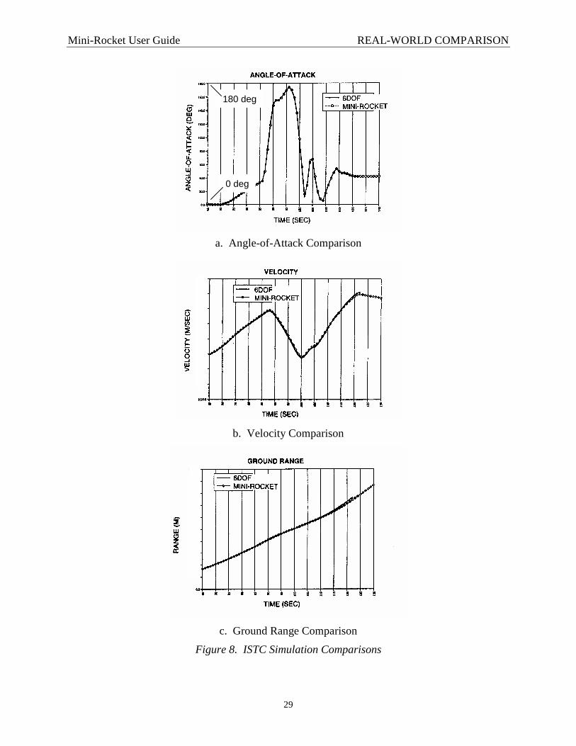
The GEMS maneuver was implemented in Mini-Rocket and the trajectories were successfully anchored to those generated by the engineering-level 6-DOF simulation used by the missile developer [3]. A comparison of simulation results is shown in Figure 8.
Mini-Rocket User Guide REAL-WORLD COMPARISON
29
180 deg
0 deg
a. Angle-of-Attack Comparison
b. Velocity Comparison
c. Ground Range Comparison
Figure 8. ISTC Simulation Comparisons

Mini-Rocket User Guide REAL-WORLD COMPARISON
30
In particular, note the very high angle-of-attack, which in effect, produced a negative thrust vector. This effective reverse thrust “wastes” energy to minimize and shape the velocity for this particular intercept. The agreement between Mini-Rocket and the 6-DOF simulation is remarkable for this complex maneuver, even though Mini-Rocket does not directly model the missile rigid body dynamics.
The ISTC subsequently used Mini-Rocket as a driver to stimulate other models and as a risk-reduction until a contractor-developed model was delivered.
5.2.2 Anti-Satellite Mission Scenario Analysis
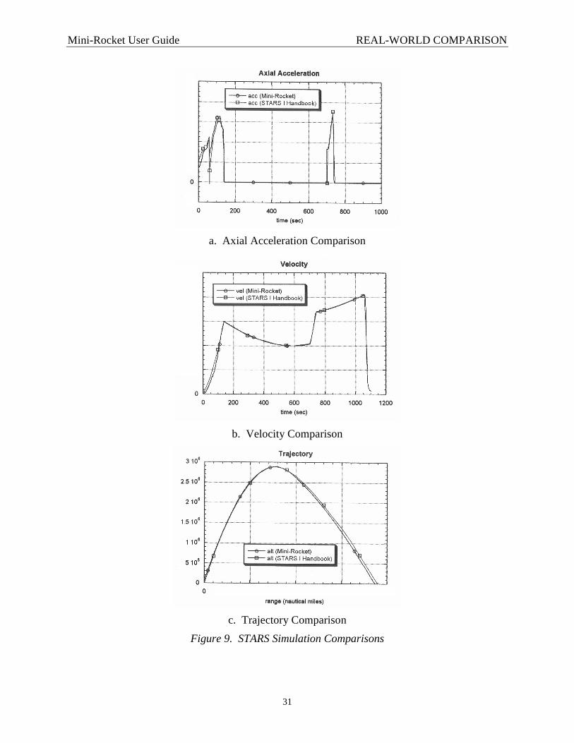
The Strategic Target System (STARS) was selected as the carrier vehicle for kinetic energy anti-satellite (ASAT) interceptor testing. In addition to being the simulation used to screen different candidate booster systems, Mini-Rocket was used to study and establish test flight scenarios. A number of constraints made configuring the scenario somewhat complicated. The ASAT kill vehicle was to be launched from the Pacific Missile Range (Hawaii) for intercepts in the vicinity of the Kwajelein Missile Range. A dog-leg maneuver had to be performed just after launch to satisfy range safety requirements. A pitch-up maneuver, late into boost, had to be performed to replicate geometry aspects of a satellite intercept. Although, Sandia National Laboratories, the STARS developer, had overall simulation responsibility with their in-house 6-DOF simulation, another simulation was needed to perform the large number of trajectory trades that were required to fully develop mission scenarios. As a first step in establishing Mini-Rocket credibility to satisfy this need, a Mini-Rocket STARS characterization was developed and compared to trajectory data in the STARS Payload Designer Handbook [4]. Results of the comparison are shown in Figure 9.
Mini-Rocket User Guide REAL-WORLD COMPARISON
31
a. Axial Acceleration Comparison
b. Velocity Comparison
c. Trajectory Comparison
Figure 9. STARS Simulation Comparisons
Mini-Rocket User Guide REAL-WORLD COMPARISON
32
The successful comparison demonstrated Mini-Rocket’s viability to rapidly screen large sets of potential trajectories that could be explored in more detail with the Sandia National Laboratory 6-DOF simulation. In addition to being successfully used for the ASAT mission trajectory studies, Mini-Rocket came to be used as a trusted simulation to address other ASAT studies, including trajectory dispersion and preliminary range safety studies.
5.2.3 EADSIM
Early versions of Extended Air Defense Simulation (EADSIM) (version 4.0 and before) did not have a simulation-based missile model per se; instead, interceptor missile trajectories were represented by table look-ups. The data in the tables were generated by external simulations. User requests for increased fidelity dictated that a missile flight model be directly incorporated into EADSIM. Speed-of-execution was a key requirement and thus precluded use of a 6-DOF representation. An embedded version of Mini-Rocket fit the requirement perfectly and was integrated into EADSIM [5]. The Mini-Rocket model augmented EADSIM with the capability to directly characterize the trajectory dynamics of interceptor missiles homing and engaging a target. In essence, each new incorporation of a missile into the EADSIM fly-out model represents another successful comparison since the performance of the Mini-Rocket-based EADSIM model is checked against external trajectory predictions in the normal course of confirming successful model installation.
5.3 A Legacy of Successful Comparisons Continues
Mini-Rocket builds on a successful legacy of accurately depicting trajectories for diverse rocket and missile applications and has established itself within the AMRDEC as the tool of choice for characterizing missile systems. As of the time of writing for this report, Mini-Rocket is being actively exploited on two key programs within the AMRDEC.
5.3.1 Extended Air Protection and Survivability Program (EAPS)
The EAPS program is developing a missile concept to protect against short-range rockets, artillery, and mortars. A key feature of the development, conducted in-house by the AMRDEC, was to prototype a design based on simulation collaboration by the missile subject matter experts. An evolving simulation, whose fidelity was consistent with the maturity of the design, was used as the central collaboration tool to document the design. The strategy was to begin the top-level aspects of the design with a reduced fidelity simulation and then mature it to a full 6-DOF as design of the missile’s subsystems progressed.
The object-oriented architecture of the CMD (described in a later section in this manual) was selected as the ideal coding platform to execute the simulation development process. Mini-Rocket, which is hosted in the CMD architecture, was used to study and assess candidate designs due to its unique combination of relatively high-fidelity (compared to conventional 3-DOF) and modest coding complexity and runtime efficiency (compared to 6-DOF). A baseline design was arrived at after extensive trade studies with Mini-Rocket and the resulting design was remodeled from a Mini-Rocket implementation to a full-up 6-DOF representation (all within the same CMD code kernel). This presented the unique opportunity to simultaneously run the Mini-Rocket-
Mini-Rocket User Guide REAL-WORLD COMPARISON
33
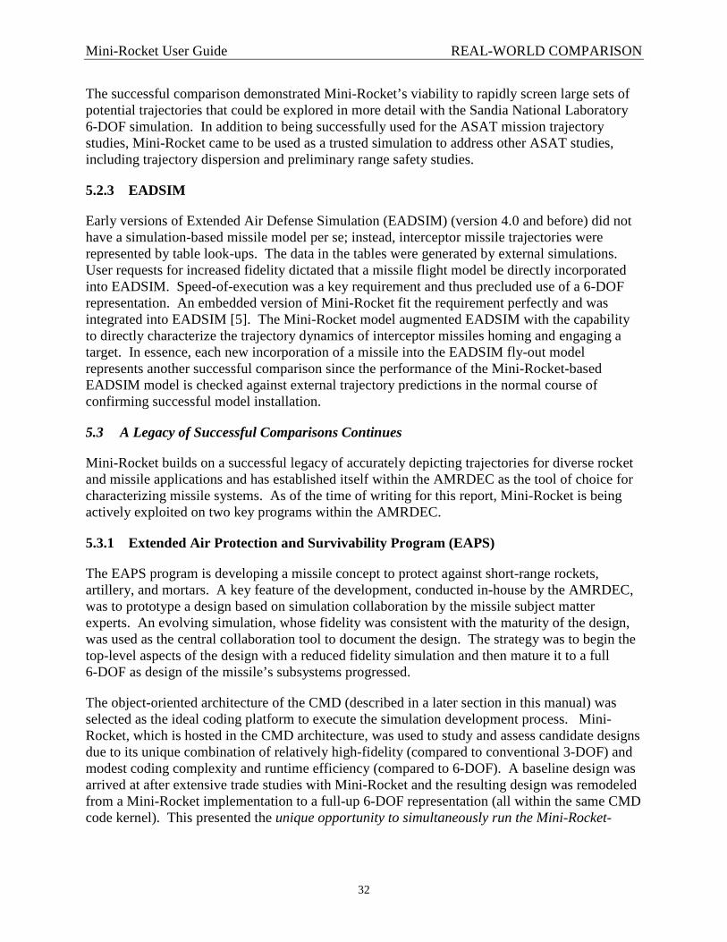
based EAPS missile in the same physical simulation as the 6-DOF-based EAPS missile (that is, they are launched at the same time and fly out simultaneously) [6].
Figure 10 shows excerpts from an animation constructed from the simultaneous simulations. Both a Mini-Rocket-based EAPS and a 6-DOF EAPS are shown flying out side-by-side, starting from launchers that are slightly offset from each other.
6DOF5DOF
a. Just After Launch
6DOF 5DOF
b) Initial Pitchover
Figure 10. EAPS Side-by-Side Simulation Comparisons (6-DOF and Mini Rocket)
Mini-Rocket User Guide REAL-WORLD COMPARISON
34
6DOF 5DOF
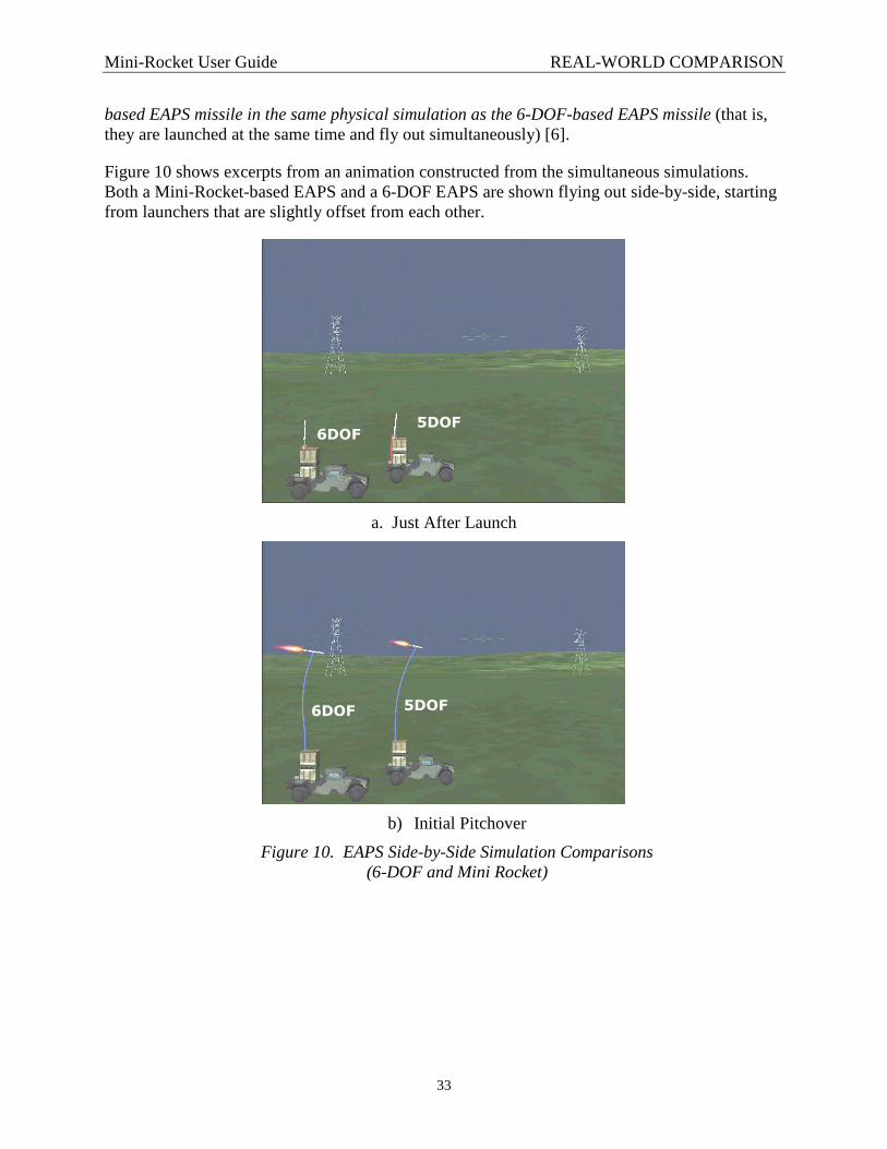
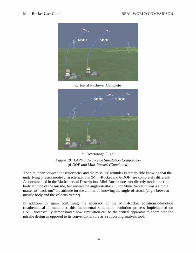
c. Initial Pitchover Complete
6DOF 5DOF
d. Downrange Flight
Figure 10. EAPS Side-by-Side Simulation Comparison (6-DOF and Mini-Rocket) (Concluded)
The similarity between the trajectories and the missiles’ attitudes is remarkable knowing that the underlying physics model characterizations (Mini-Rocket and 6-DOF) are completely different. As documented in the Mathematical Description, Mini-Rocket does not directly model the rigid body attitude of the missile, but instead the angle-of-attack. For Mini-Rocket, it was a simple matter to “back-out” the attitude for the animation knowing the angle-of-attack (angle between missile body and the velocity vector).
In addition to again confirming the accuracy of the Mini-Rocket equations-of-motion (mathematical formulation), this incremental simulation evolution process implemented on EAPS successfully demonstrated how simulation can be the central apparatus to coordinate the missile design as opposed to its conventional role as a supporting analysis tool.

Mini-Rocket User Guide REAL-WORLD COMPARISON
35
5.3.2 Interactive Distributed Engineering Evaluation and Analysis Simulation (IDEAAS)
IDEEAS is a tactical missile constructive simulation that incorporates interactive models of all the tactical battlefield elements including shooters (missiles), surveillance and fire control radar, and battle management. A key component of IDEEAS is a missile server that generates, on-demand, tactical missile representations. It was not important for this missile-server to simulate the onboard missile subsystems; the key IDEEAS requirement for a missile model is to accurately depict trajectories that, in turn, stimulate or drive the other battlefield elements. Mini-Rocket’s level of fidelity was ideal for this requirement, providing runtime efficiency without undue complexity, In addition, Mini-Rocket, with its underlying CMD object-oriented kernel could be readily embedded into IDEEAS. Because IDEEAS is Java-based, the Mini-Rocket model algorithms were refactored in Java, with an identical architecture as the C++ model. The object-oriented simulation kernel in CMD is programming language independent and was already coded in Java (as well as other languages) so it was a straightforward exercise to convert the model to Java. The Java-based Mini-Rocket was easily wrapped with a simple, but powerful, interface that could be called by the IDEEAS executive to instantiate (create) a missile object [7]. The exact missile being simulated is specified via the conventional Mini-Rocket input file described in this manual.
A Mini-Rocket-based missile model must have traceability to the original design before its missile server representation can be used in IDEEAS. One of the more challenging models successfully implemented in IDEEAS was a vertically-launched ground-to-ground missile. For long-range intercepts, the trajectory is “lofted” so that lift can sustain a relatively long flight. Successful comparison to the originating design activity’s 6-DOF simulation is shown in Figure 11 for this scenario.
Figure 11. Ground-to-Ground Missile Simulation Comparison

Mini-Rocket User Guide REAL-WORLD COMPARISON
36
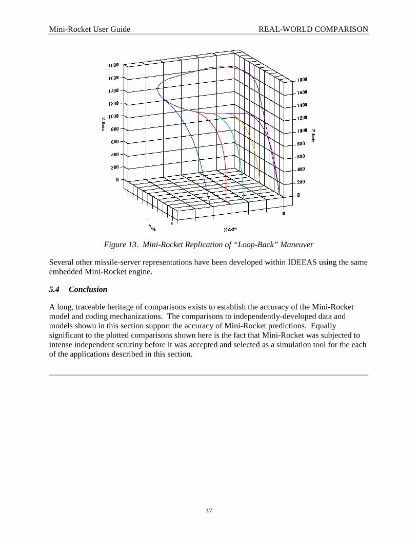
Much more stressing from a modeling view are short-range trajectories. The missile is capable of accomplishing very short range intercepts by flying out and “looping” back. A simulation-generated example from the prime contractor developer is shown in Figure 12. Normally, this would be very difficult to simulate given the complexity of the commands to execute the maneuver.
Figure 12. Prime Contractor Simulation Depiction of Complex “Loop-Back” Maneuver
The unique osculating plane formulation behind Mini-Rocket made it relatively simple to replicate the trajectory since a left/right and up/down frame-of-reference is used to specify steering in the input data. Example Mini-Rocket-generated results are shown in Figure 13 which very closely replicated the missile’s performance.
Mini-Rocket User Guide REAL-WORLD COMPARISON
37
Figure 13. Mini-Rocket Replication of “Loop-Back” Maneuver
Several other missile-server representations have been developed within IDEEAS using the same embedded Mini-Rocket engine.
5.4 Conclusion
A long, traceable heritage of comparisons exists to establish the accuracy of the Mini-Rocket model and coding mechanizations. The comparisons to independently-developed data and models shown in this section support the accuracy of Mini-Rocket predictions. Equally significant to the plotted comparisons shown here is the fact that Mini-Rocket was subjected to intense independent scrutiny before it was accepted and selected as a simulation tool for the each of the applications described in this section.

Mini-Rocket User Guide HOW MINI-ROCKET WAS BUILT
38
6 HOW MINI-ROCKET WAS BUILT
Mini-Rocket was built with C++ Model Developer . CMD is an open-source C++ source code based environment for building simulations of systems described by time-based differential equations. The principal design objective behind CMD is to provide a tool to go from mathematical representation to working, extensible C++ code with a minimum amount of effort.
The heart of CMD is a powerful Object-Oriented Simulation Kernel (OSK) that represents significant technology advances in the application of object-oriented principles to simulation development and design [8]. The OSK architecture is language-independent and can serve as the basis for recreating Mini-Rocket in other computer languages as shown in Figure . In fact, Mini-Rocket as described in this User Guide has been replicated in Java and Python. Standalone programs in these languages use the same identical input data file as the CMD-based executable version.
Object-Oriented Simulation Kernel• Train-of-objects• Seamless mixing of hybrid models
C++ Model Developer JavaPython
Mini-RocketMini-Rocket Mini-Rocket
EAPS Concept 6DOF
Architecture• Language Independent
Coding Mechanism• Model Independent
ModelsCKEM 6DOFMLRS 6DOF IDEEASAMCODE
Figure 14. Object-Oriented Simulation Architecture and Simulation Construction Hierarchy
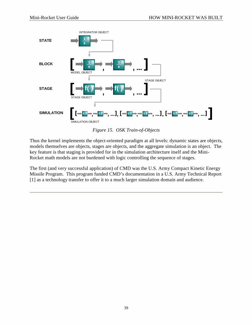
A key feature and state-of-the art advance of the OSK is the train-of-objects architecture depicted in Figure . The OSK’s unique train-of-objects architecture is well suited for the multiple stage modeling required by Mini-Rocket. The organization of the entities used by the kernel is shown in Figure . At a micro-level, each state (that is each individual integrator) is a C++ object (STATE in the figure). One or more states are combined, connected by algorithms for their derivatives, into a block (or model). Several models are combined into a stage. Finally, a series of stages are combined in a list. A simulation class in the kernel then decomposes this “list-of-lists-of-lists” to execute the models in the desired order (specified by their order in the lists) and, within each model, the appropriate methods described in the previous section.
Mini-Rocket User Guide HOW MINI-ROCKET WAS BUILT
39
1s1s1s
STATE
1s
1s, , ...[ ]1
s1s
1s1s, , ...[ ]
, , ...[ ]f( ) f( ), , ...[ ]f( ) f( )
, , ...[ ]f( ) f( ) , , ...[ ]f( ) f( ) , , ...[ ]f( ) f( ), ,[ ], , ...[ ]f( ) f( ) , , ...[ ]f( ) f( ) , , ...[ ]f( ) f( ), ,[ ]
BLOCK
STAGE
SIMULATION
INTEGRATOR OBJECT
MODEL OBJECT
STAGE OBJECT
STAGE OBJECT
SIMULATION OBJECT
Figure 15. OSK Train-of-Objects
Thus the kernel implements the object-oriented paradigm at all levels: dynamic states are objects, models themselves are objects, stages are objects, and the aggregate simulation is an object. The key feature is that staging is provided for in the simulation architecture itself and the Mini-Rocket math models are not burdened with logic controlling the sequence of stages.
The first (and very successful application) of CMD was the U.S. Army Compact Kinetic Energy Missile Program. This program funded CMD’s documentation in a U.S. Army Technical Report [1] as a technology transfer to offer it to a much larger simulation domain and audience.

Mini-Rocket User Guide SUMMARY
40
7 SUMMARY
Mini-Rocket fills an important simulation niche as shown by the vast number of applications and tasks where it has been utilized over a number of years. In these analyses, the fidelity requirements are not satisfied with a 3-DOF simulation, but the complexity, and associated resource requirements, of a 6-DOF far exceed what is required to satisfy analysis needs. With the progressive advent of faster and faster computing power, the difficulty with using a 6-DOF (over a 3-DOF) is not any longer computer runtime but, instead, the far greater complexity of configuring input for the 6-DOF owing to the detail of its underlying subsystem models. Mini-Rocket resolves this issue, effectively having a broad subset of the fidelity of a 6-DOF simulation, but with the resource requirements (runtime and input complexity) of a 3-DOF.
An integral part of the Mini-Rocket application success story is its malleability to be easily modified and augmented. This report documents a packaged, standalone version of the algorithms that comprise Mini-Rocket and this packaged tool has been, and will continue to be, used by a wide audience. But, perhaps more importantly, a broader application arena for Mini-Rocket is its flexibility to be molded and configured to address specific analysis and modeling situations. The algorithm code is relatively short, concise, and readily understood, which makes it very easy to modify for a broad domain of needs. The inherent modular nature of the object-oriented simulation kernel behind CMD was a great medium for exploiting the power of the algorithms behind Mini-Rocket. It is anticipated that Mini-Rocket will continue to morph into even more application areas and coding mediums in the future.
In summary, Mini-Rocket is a versatile tool having the distinguishing characteristics of a high degree of fidelity given its very modest complexity (the unique mathematical formulation), a long legacy of successful application to establish credibility, and a flexible code structure that enables it to be rapidly configured or modified for a wide variety of custom applications.

Mini-Rocket User Guide REFERENCES
41
REFERENCES
1. Sells, H.R., Sanders, G.A., Snyder, G., Hester, J.W., and Painter, L. 2005. “C++ Model Developer (CMD) User Guide.” U.S. Army Technical Report AMR-SG-05-12, April 2005.
2. Sells, H.R., “Comparison of KDEC Aries Test Article Trajectories to Off-Line Model,” Teledyne Brown Engineering technical letter SSDCSY-93-61AB01-1533100801-0573 to Ms. Jackie Steele, U.S. Army Space and Strategic Defense Command, 10 August 1993.
3. Sells, H.R., “Mini-Rocket GEMS Implementation,” report delivered to Mr. Dan Bowman, Teledyne Brown Engineering, 1995.
4. Sells, H.R., and Cupples, M., “ASAT Test Mission Scenario Analysis – Trajectory Studies,” report for U.S. Army Space and Strategic Defense Command, contract DASG60-97-C-0054, 21 January 1998.
5. Extended Air Defense Simulation (EADSIM) Methodology Manual, Section 5.9, “Interceptor Missile Flight.” Teledyne Brown Engineering, Huntsville, AL, 1995.
6. Sells, H.R., and Leopard, P., “EAPS Simulation Build 6 – 6-DOF Simulation Description and Delivery,” report delivered at EAPS Simulation Working Group #27 to Mr. George Sanders, AMRDEC, 1 March 2007.
7. Sells, H.R., “Java Mini-Rocket Live Code Demo,” report and model delivery to Mr. Ron Saylor, AMRDEC, 9 December 2005.
8. Sells, H.R., Sanders, G., and Saylor, R., “An Object-Oriented Simulation Kernel for a Large Spectrum of Simulations,” Summer Computer Simulation Conference, Society for Computer Simulation, 2006, Calgary, Alberta.
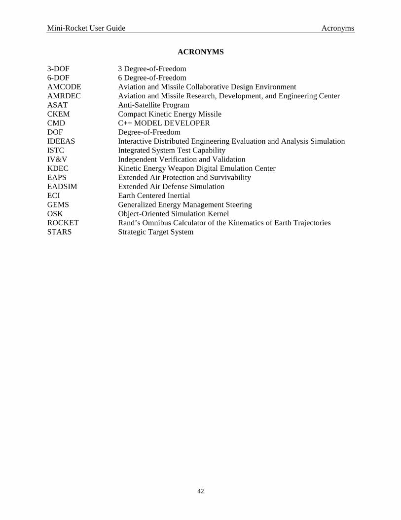
Mini-Rocket User Guide Acronyms
42
ACRONYMS
3-DOF 3 Degree-of-Freedom 6-DOF 6 Degree-of-Freedom AMCODE Aviation and Missile Collaborative Design Environment AMRDEC Aviation and Missile Research, Development, and Engineering Center ASAT Anti-Satellite Program CKEM Compact Kinetic Energy Missile CMD C++ MODEL DEVELOPER DOF Degree-of-Freedom IDEEAS Interactive Distributed Engineering Evaluation and Analysis Simulation ISTC Integrated System Test Capability IV&V Independent Verification and Validation KDEC Kinetic Energy Weapon Digital Emulation Center EAPS Extended Air Protection and Survivability EADSIM Extended Air Defense Simulation ECI Earth Centered Inertial GEMS Generalized Energy Management Steering OSK Object-Oriented Simulation Kernel ROCKET Rand’s Omnibus Calculator of the Kinematics of Earth Trajectories STARS Strategic Target System

Mini-Rocket User Guide APPENDIX 1: MAKING PLOTS
APPENDIX 1 MAKING PLOTS

Mini-Rocket User Guide APPENDIX 1 – MAKING PLOTS
A-1
APPENDIX 1 – MAKING PLOTS
Although not a part of Mini-Rocket itself, a simple-to-use plotter is provided that is compatible with the output files generated at runtime. The name of the plotter is wxpp. wxpp is a quick-and-easy interactive, scriptable 2-d x-y plotting tool. It is primarily designed to expedite the rapid visualization of simulation results as quickly as possible without the necessity of navigating selection menus or other options. wxpp is fully scriptable since it is command-line driven with options specified in an ASCII-text configuration file. Plots can be totally configured and generated from simple scripts. wxpp produces production-quality, high-resolution plots suitable for direct incorporation into reports or briefings. Some of its most basic capabilities are briefly described here and should be adequate for use with Mini-Rocket.
1.1 Installing the Plotter wxpp is a single standalone Windows “.exe” file so it can easily be installed and used. Make sure the file “wxpp.txt” is also in the same directory.
1.2 Basic Usage The most fundamental way to use wxpp is from the command line to generate plots lightening fast. The environmental variable DATAFILE specifies the filename of the data to be plotted. This can be set from the command line as: C:> set DATAFILE=OutputRun0.dat Within the data file, data to be plotted is formatted as 0 t rng h mach gammad v tx alph 0.000 0.00 0.00 0.00 40.00 0.01 0.0 0.00 0.770 450.99 372.96 5.40 39.50 1828.42 0.0 0.00 1.000 775.35 640.11 5.41 39.45 1828.69 1259.0 0.00 The contents of the first line is ignored and can contain any text (maybe some information about the file’s contents for instance). The second line contains the names of the fields that can be plotted. Each name corresponds to a column of data in the subsequent line. The remaining lines of the file contain rows of data for each field. The available fields for plotting can be queried by C:> wxpp
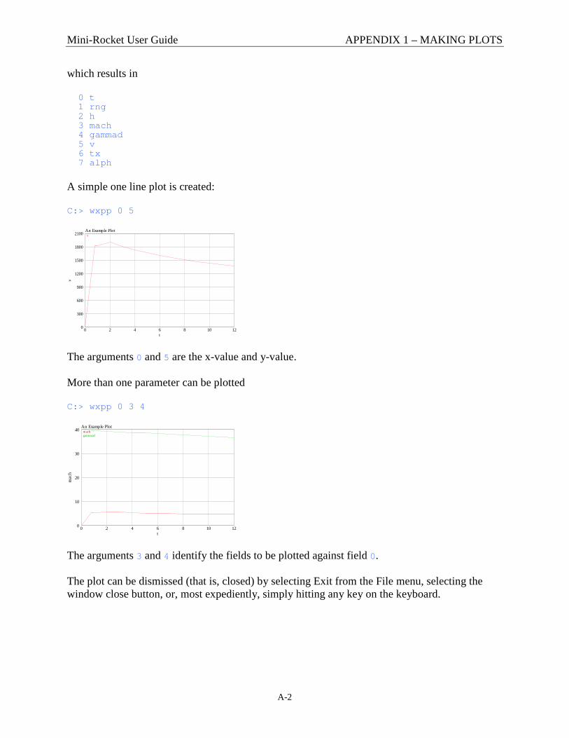
Mini-Rocket User Guide APPENDIX 1 – MAKING PLOTS
A-2
which results in 0 t 1 rng 2 h 3 mach 4 gammad 5 v 6 tx 7 alph A simple one line plot is created: C:> wxpp 0 5
An Example Plot
0 2 4 6 8 10 12t
0
300
600
900
1200
1500
1800
2100
v
v
The arguments 0 and 5 are the x-value and y-value. More than one parameter can be plotted C:> wxpp 0 3 4
An Example Plot
0 2 4 6 8 10 12t
0
10
20
30
40
ma
ch
machgammad
The arguments 3 and 4 identify the fields to be plotted against field 0. The plot can be dismissed (that is, closed) by selecting Exit from the File menu, selecting the window close button, or, most expediently, simply hitting any key on the keyboard.
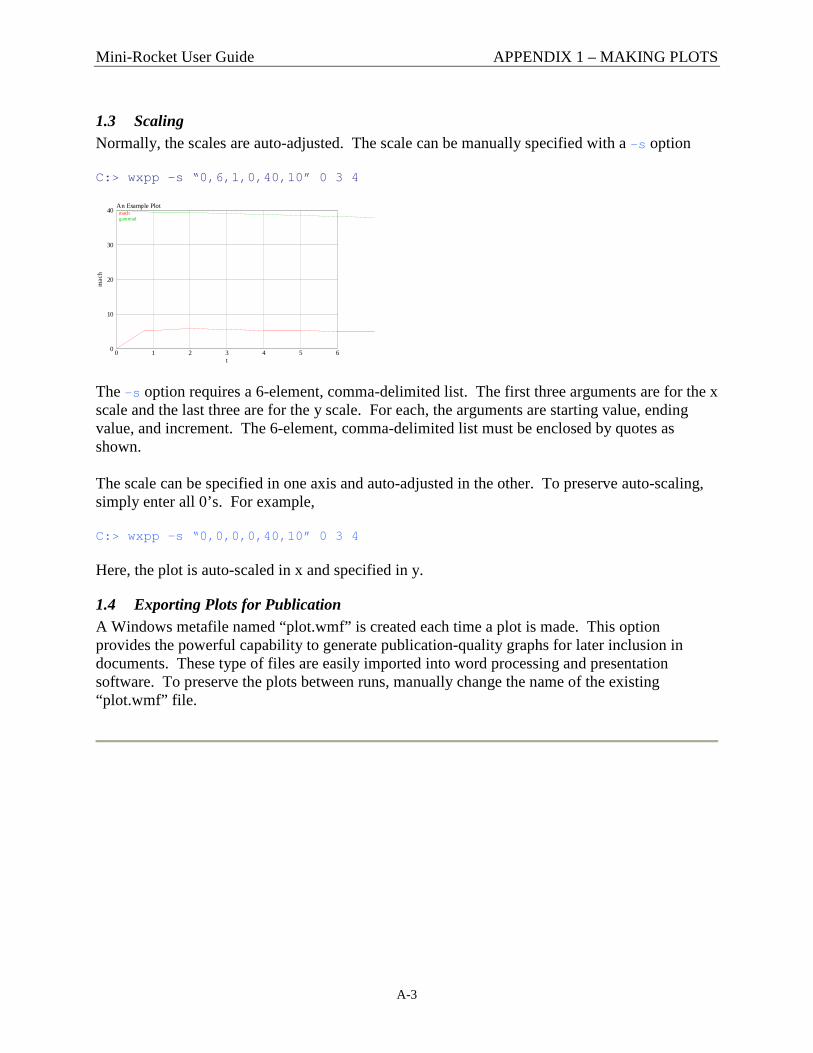
Mini-Rocket User Guide APPENDIX 1 – MAKING PLOTS
A-3
1.3 Scaling Normally, the scales are auto-adjusted. The scale can be manually specified with a -s option C:> wxpp -s “0,6,1,0,40,10” 0 3 4
An Example Plot
0 1 2 3 4 5 6t
0
10
20
30
40
ma
ch
machgammad
The -s option requires a 6-element, comma-delimited list. The first three arguments are for the x scale and the last three are for the y scale. For each, the arguments are starting value, ending value, and increment. The 6-element, comma-delimited list must be enclosed by quotes as shown. The scale can be specified in one axis and auto-adjusted in the other. To preserve auto-scaling, simply enter all 0’s. For example, C:> wxpp -s “0,0,0,0,40,10” 0 3 4 Here, the plot is auto-scaled in x and specified in y.
1.4 Exporting Plots for Publication A Windows metafile named “plot.wmf” is created each time a plot is made. This option provides the powerful capability to generate publication-quality graphs for later inclusion in documents. These type of files are easily imported into word processing and presentation software. To preserve the plots between runs, manually change the name of the existing “plot.wmf” file.
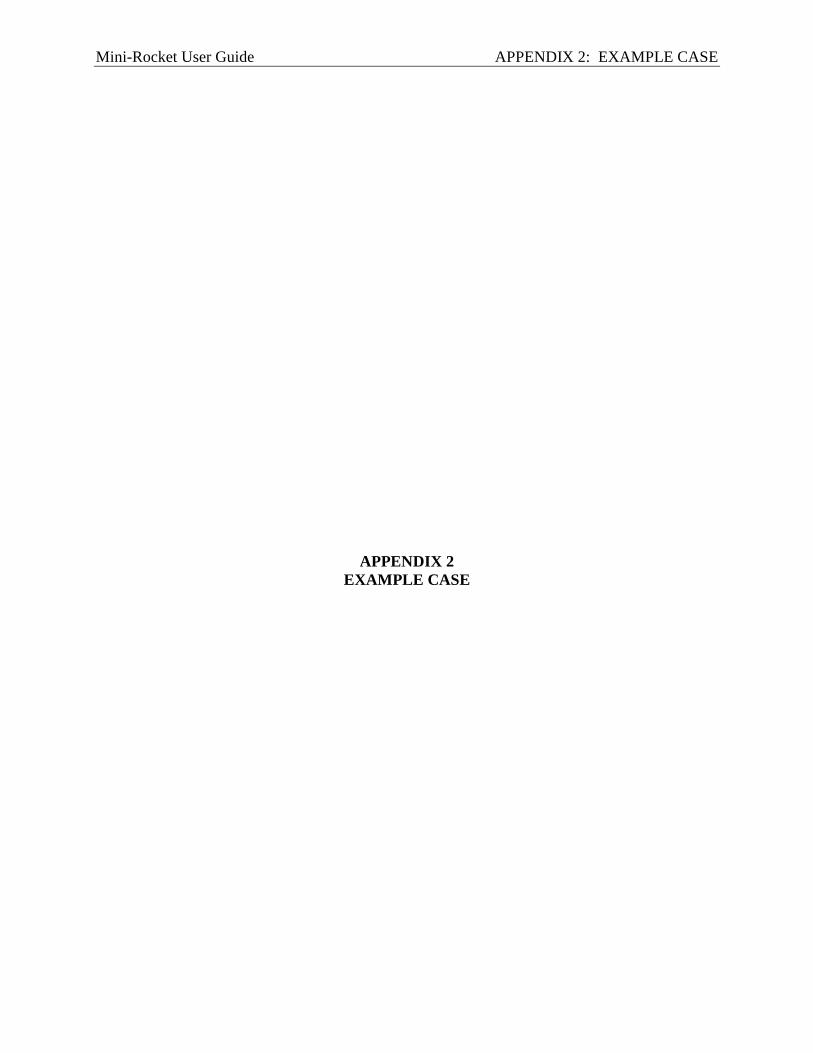
Mini-Rocket User Guide APPENDIX 2: EXAMPLE CASE
APPENDIX 2 EXAMPLE CASE

Mini-Rocket User Guide APPENDIX 2 – EXAMPLE CASE
B-1
APPENDIX 2 - EXAMPLE CASE
An example case is shown here to acquaint the user with typical output and to illustrate Mini-Rocket functionality. The input for this example is exactly that used to describe the input in the previous “Input Data File” section of this report. The missile being simulated is a hypothetical three-stage exo-atmospheric missile vertically launched from the ground. Program operation in a Windows environment is shown here. Of course, Mini-Rocket is cross-platform since it is written in standard C++ and is operated from a simple console interface. Operation proceeds as described in section “Installation.”
The input file, rocket.dat, is the same as described earlier.
First, the contents of the input data file are echoed (after the standard program output banner).

Mini-Rocket User Guide APPENDIX 2 – EXAMPLE CASE
B-2
Computed program output to the console consists of those parameters specified for output in the input data file in columnar format. Each row begins with the time followed by parameter values at that time.

Mini-Rocket User Guide APPENDIX 2 – EXAMPLE CASE
B-3
In this case, time is followed by range, altitude, velocity, flight path angle, and angle-of-attack. A message is printed at stage separation (section change) events. Console output is merely a convenience to see that the program ran and to quickly observe, in a coarse sense, key flight parameters. Beyond that, it is difficult to discern much more from the console output. The primary output record is constrained in a separate output text file. This file is ASCII-text and can be opened with any simple text editor. The name of the file is that specified with the identifier fname in the input data file. An excerpt from the data file is as shown.
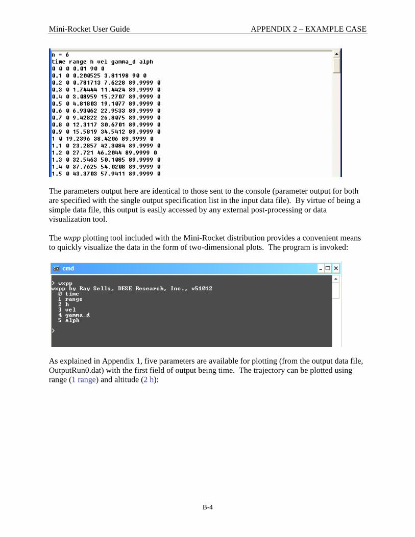
Mini-Rocket User Guide APPENDIX 2 – EXAMPLE CASE
B-4
The parameters output here are identical to those sent to the console (parameter output for both are specified with the single output specification list in the input data file). By virtue of being a simple data file, this output is easily accessed by any external post-processing or data visualization tool. The wxpp plotting tool included with the Mini-Rocket distribution provides a convenient means to quickly visualize the data in the form of two-dimensional plots. The program is invoked:
As explained in Appendix 1, five parameters are available for plotting (from the output data file, OutputRun0.dat) with the first field of output being time. The trajectory can be plotted using range (1 range) and altitude (2 h):

Mini-Rocket User Guide APPENDIX 2 – EXAMPLE CASE
B-5
The resulting plot is:
The action of the three stages can easily be discerned in the velocity vs. time plot (wxpp 0 3):
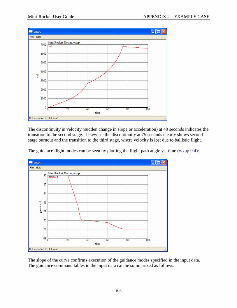
Mini-Rocket User Guide APPENDIX 2 – EXAMPLE CASE
B-6
The discontinuity in velocity (sudden change in slope or acceleration) at 40 seconds indicates the transition to the second stage. Likewise, the discontinuity at 75 seconds clearly shows second stage burnout and the transition to the third stage, where velocity is lost due to ballistic flight. The guidance flight modes can be seen by plotting the flight path angle vs. time (wxpp 0 4):
The slope of the curve confirms execution of the guidance modes specified in the input data. The guidance command tables in the input data can be summarized as follows:

Mini-Rocket User Guide APPENDIX 2 – EXAMPLE CASE
B-7
time (sec) stage guidance mode
0-20 1 vertical launch, ballistic flight 20-30 1 pitch over at 1 deg/sec 30-40 1 pitch over to 75 deg flight path angle 40-60 2 fly ballistically 60-75 2 accelerate down (-z direction) at 11 m/sec2 75-100 3 fly ballistically
The maneuvers are verified by reconciling the entries in the table to the behavior of the plot. The flight path stays constant at 90 degrees from vertical launch (0 to 20 seconds). The 1 degree/second pitch down is clearly seen as the flight angle goes from 90 to 80 degrees (change of 10 degrees) in 10 seconds (20 to 30 seconds). Consistent with an equivalent time constant of 1 second, the flight path angle quickly changes to 75 and holds there (30 to 40 seconds). The flight path angle slowly decreases as the missile flies ballistically and slowly pitches down due to gravity (40 to 60 seconds). A downward acceleration is clearly observed in response to the acceleration guidance command (60 to 75 seconds). Again, the downward pull of gravity is seen by the slowly decreasing flight angle during the final ballistic flight segment (75 to 100 seconds). It is usually a good “sanity” check to confirm that the vehicle’s motion was “well-behaved” – that is, the vehicle was not tumbling! An easy way to check this is to plot the Angle-of-Attack (AOA):
It is quickly seen that the AOA stayed within a reasonable limit for the entire flight. Again, the behavior in the table can be reconciled to the plot. The AOA was zero after launch until the missile began to pitch over (0 to 20 seconds). The AOA becomes non-zero for the 1 degree/second pitchover (20 to 30 seconds). Notably, the AOA saturates (that is, reaches its

Mini-Rocket User Guide APPENDIX 2 – EXAMPLE CASE
B-8
specified maximum limit of 9 degrees, alphmax in the data file) to fully accomplish the 75-degree flight path angle (30 to 40 seconds). Again the AOA is zero while the missile flies ballistically (40 to 60 seconds). The AOA becomes non-zero for the downward acceleration maneuver (60 to 75 seconds). Finally, the AOA is zero for the ballistic duration of the flight (75 to 100 seconds). Of course, the parameters that can be plotted are not limited to those shown here; a full range of other parameters can be specified for plotting via selection in the input data. As shown by this example, Mini-Rocket in tandem with quick turnaround plotting tool (like wxpp) form a potent analysis tool to quickly determine missile performance and play “what-ifs” by perturbing the parameters that characterize the missile. A myriad of analyses can be performed using the cycle of steps shown in this example.

Mini-Rocket User Guide APPENDIX 2 – EXAMPLE CASE
B-9
THIS PAGE LEFT INTENTIONALLY BLANK
Dist-1
INITIAL DISTRIBUTION LIST
Copies Weapon Systems Technology Information Electronic Analysis Center Ms. Vakare Valaitis 1901 N. Beauregard Street, Suite 400 [email protected] Alexandria, VA 22311-1720 Defense Technical Information Center Jack Rike Electronic 8725 John J. Kingman Rd., Suite 9044 [email protected] Fort Belvoir, VA 220060-6218 Aviation Advanced Design Team Dr. Nancy M. Bucher Electronic U.S. Army Aviation and Command (AMCOM) [email protected] Aeroflightdynamics Directorate (AFDD) Ames Research Center, M/S 219-3 Moffett Field, CA 94035-1000 Commander, U.S. Army ARDEC Dan Ericson Electronic ATTN: AMSRD-AR-AIS-SA [email protected] Picatinny Arsenal, NJ 07806-5000 DESE Research, Inc. Mr. Ray Sells Electronic 315 Wynn Drive [email protected] Huntsville, AL 35805 Mr. Michael Fennell [email protected] George C. Marshall Space Flight Center Jim McCarter Electronic Aerospace Engineer [email protected] Mail Code EV42 Marshall Space Flight Center, AL 35812 Professor, Aerospace Engineering Dr. Roy J. Hartfield, Jr. Electronic 328 Aerospace Engineering Building [email protected] Auburn University, AL 35849-5338 Sensors Integration and Test and Evaluation George W. Snyder, Director Electronic Directorate [email protected] SMDC-RDTC-TE Building 5220 U.S. Army Space and Missile Defense Command USASMDC/ARSTRAT Redstone Arsenal, AL 35898

Dist-2
INITIAL DISTRIBUTION LIST (CONTINUED) Copies University of Alabama in Huntsville Dr. Robert A. Frederick Electronic Propulsion Research Center [email protected] 5000 Technology Drive, TH S231 [email protected] Huntsville, AL 35899 University of Alabama in Huntsville Dr. D. Brian Landrum Electronic Propulsion Research Center [email protected] 5000 Technology Drive, S234 Huntsville, AL 35899 University of Alabama in Huntsville Dr. Nathan J. Slegers Electronic Propulsion Research Center [email protected] 5000 Technology Drive, N266 Huntsville, AL 35899 AMSRD-AMR Dr. William McCorkle Electronic [email protected] AMSRD-AMR-AS-TI Mr. Ron Schmalbach Electronic [email protected] AMSRD-AMR-CS-IC Electronic AMSRD-AMR-PS Mr. C. Steven Cornelius Electronic [email protected] AMSRD-AMR-PS-PT Dr. Jay Lilley Electronic [email protected] Mr. Scott Michaels Electronic [email protected] AMSRD-AMR-SG Dr. Robin B. Buckelew Electronic [email protected]

Dist-3
INITIAL DISTRIBUTION LIST (CONTINUED) Copies AMSRD-AMR-SG-RF Mr. Michael Christian Electronic [email protected] Mr. Chris Hamner Electronic [email protected] Mr. Jim Mullins Electronic [email protected] Ms. Janice C. Rock Electronic [email protected] Dr. Brian Smith Electronic [email protected] AMSRD-AMR-SG-SD Dr. James Bauman Electronic [email protected] Mr. Jeffrey W. Hester Electronic [email protected] Mr. Phillip N. Jenkins Electronic [email protected] Mr. Bill Nourse Electronic [email protected] Ms. Loretta Painter Electronic [email protected] Mr. Heniz Sage Electronic [email protected] Mr. Alfred Wright Electronic [email protected] AMSRD-AMR-SS Mr. Richard Kretzschmar Electronic [email protected] Mr. Greg B. Tackett Electronic [email protected] AMSRD-AMR-SS-AE Mr. Charlie Derrick Electronic [email protected] Ms. Laurie Fraser Electronic [email protected] Mr. Tim McKelvy Electronic [email protected] Mr. George A. Sanders Electronic [email protected] Mr. Ron Saylor Electronic [email protected]

Dist-4
INITIAL DISTRIBUTION LIST (CONTINUED) Copies AMSRD-AMR-SS-AT Mr. Lamar Auman Electronic [email protected] Mr. Don Ferguson Electronic [email protected] Ms. Amanda Horton Electronic [email protected] Dr. James Keenan Electronic [email protected] Ms. Melissa McDaniel Electronic [email protected] Mr. David B. Riddle Electronic [email protected] Mr. Clark B. Roberts Electronic [email protected] Mr. Brett Wilks Electronic [email protected] AMSRD-AMR-SS-AV Mr. Steve Low Electronic [email protected] AMSRD-AMR-SS-EG Mr. Brian M. Harrison Electronic [email protected] Ms. Ann Kissell Electronic [email protected] AMSRD-AMR-SS-MD Mr. Tim Carroll Electronic [email protected] Mr. Mark Horton Electronic [email protected] AMSRD-AMR-SS-TM Mr. Keith Jadus Electronic [email protected] Mr. Blake Haynes Electronic [email protected] Mr. Scott Speigle Electronic [email protected] Mr. George Wiggs Electronic [email protected] AMSRD-L-G-I Ms. Anne Lanteigne Electronic [email protected]