DESINGNING GROUP ACCEPTANCE SAMPLING … · DESIGNING GROUP ACCEPTANCE SAMPLING PLANS FORTHE WEIBULL AND GAMMA DISTRIBUTION USING MINIMUM ANGLE METHOD Dr. A. R. Sudamani Ramaswamy

International Journal of Mathematics and Statistics Studies

Vol.1, No. 4, pp.23-36, December 2013

Published by European Centre for Research Training and Development UK (www.ea-journals.org)

23

DESIGNING GROUP ACCEPTANCE SAMPLING PLANS FORTHE WEIBULL AND

GAMMA DISTRIBUTION USING MINIMUM ANGLE METHOD

Dr. A. R. Sudamani Ramaswamy

Associate professor, Department of Mathematics, Avinashilingam University,

Coimbatore – 641043(T.N), India..

R. Sutharani

Assistant professor of Mathematics, Coimbatore Institute of Technology,

Coimbatore-641014(T.N),India

ABSTRACT: In this paper, minimum angle method is introduced to find the parameters of a

group acceptance sampling plan in which the truncated lifetimes follows a Weibull and gamma

distribution. The values of operating ratio corresponding to the producer’s risk and consumer’s

risk are calculated and using minimum angle method and the minimum angle θ is found. Tables

are constructed and examples are provided.

KEYWORDS : Weibull and gamma distribution, Group acceptance sampling: producer’s risk,

Operating characteristics, Producer’s risk, Minimum angle method.

INTRODUCTION

The sampling procedure is turned out to be a life testing, when the quality characteristics are

related to product lifetime. It is very often not to observe a failure for a highly reliable product

within available experimental time duration.

The ordinary acceptance sampling plan for different distributions have been developed by many

researchers including, Kantam et al, [1].Baklizi [2], Balakrishnan et al, [3] and Lio et al. [4] and

[5]. However, it requires more cost time and observation to collect the sample items for making a

decision of either accepting or rejecting the lot of products. An acceptance sampling plan

involves quality contracting on product orders between the producers and consumers. . In order

to fix the acceptance number in a sampling plan is very difficult. By the minimum angle criteria

the optimum value of the acceptance number was designed. In this paper designing group

acceptance sampling plan under weibull and gamma distribution using minimum angle method

is presented. GASP plans having minimum angle by keeping the producer’s risk below 5%

and consumer’s risk below 10% for specified AQL and LQL were presented.

WEIBULL AND GAMMA DISTRIBUTION

Weibull Distribution:

The cumulative distribution function (cdf) of the weibull distribution is given by

http://www.ea-journals.org/




24

F ( t, ) = 1 - (1)

Where is the scale parameter and m is the shape parameter and it is equal to 2

GAMMA DISTRIBUTION: The cumulative distribution function (cdf) of the exponential distribution is given by

!/1),(

1

0

j

jt

jt

etF (2)

It is further observed that the weibull and gamma distribution can be used quite effectively in

many circumstances, in place of lognormal or generalized Rayleigh distribution also. The

closeness properties with other distributions, Statistical inferences, order statistics, have been

discussed by several authors. The readers are referred to the recent review article by Gupta and

Kundu [6] for a current account on the generalized exponential distribution.

Operating Characteristics Function:

The probability of acceptance can be regarded as a function of the deviation of the

specified value 0 of the mean from its true value . This function is called Operating

Characteristic (OC) function of the sampling plan. When the sample size n = rg is known,

we can able to find the probability of acceptance of a lot when the quality of the product is

sufficiently good. Using the probability of acceptance the corresponding to producer’s risk

and consumer’s risk the values are tabulated to calculate the minimum angle method.

Notation:

g - Number of groups

r - Number of items in a group

n - Sample size

c - Acceptance number

t0 - Termination time

a - Test termination time multiplier

m - Shape parameters

β - Consumer’s risk

P - Failure probability

L (p) - Probability of acceptance

- Mean life

0 - Specified life

θ - Minimum angle

δ - Shape parameter

Group Acceptance Sampling (Gasp) Under Weibull And Gamma Distribution:

A product is considered as good and acceptable for consumer’s use, if the true value which is

the median of the lifetime distribution of a product is not smaller than the specified median value





25

0. If the actual value is smaller than value 0. The following GASP is proposed based on the

truncated life test:

1. Select the number of groups g and allocate predefined r items to each group so that the sample

size for a lot will be n = g. r.

2. Select the acceptance number c for a group and the experiment time t0.

3. Perform the experiment for the g groups simultaneously and record the number of failures for

each group.

4. Accept the lot if atmost c failures occur in each of all groups.

5. Terminate the experiment if more than c failures occur in any group and reject the lot.

The probability of rejecting a good lot is called the producer’s risk, whereas it is represented as

α. The probability of accepting a bad lot is known as the consumer’s risk, which is represented as

β. We will determine the number of groups g in the proposed sampling plan so that the

consumer’s risk does not exceed the value β = 0.10 since the lot size is large enough; we

can use the binomial distribution to develop the GASP. According to the GASP the lot of

products is accepted only if there are atmost c failures observed in each of the g groups. The

probability of acceptance of GASP is given by

L ( p ) ----------------(3)

Where p is the probability that an item in a group fails before the termination time

to = ao.

MINIMUM ANGLE METHOD

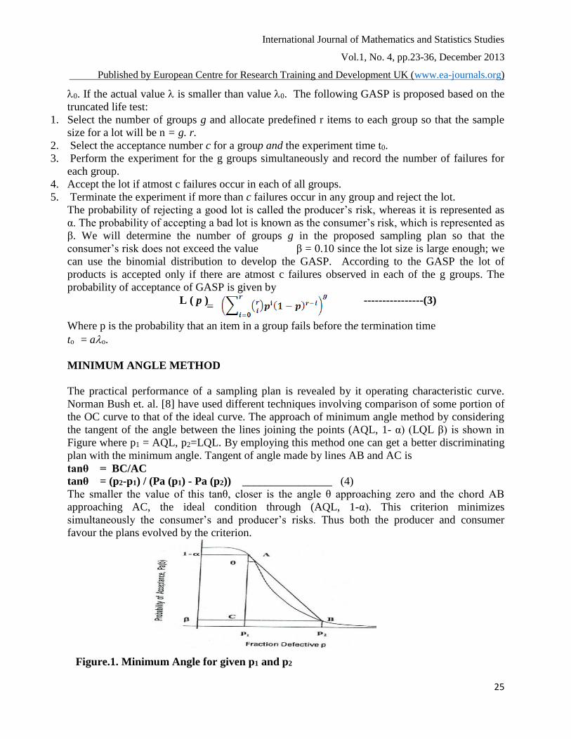
The practical performance of a sampling plan is revealed by it operating characteristic curve.

Norman Bush et. al. [8] have used different techniques involving comparison of some portion of

the OC curve to that of the ideal curve. The approach of minimum angle method by considering

the tangent of the angle between the lines joining the points (AQL, 1- α) (LQL β) is shown in

Figure where p1 = AQL, p2=LQL. By employing this method one can get a better discriminating

plan with the minimum angle. Tangent of angle made by lines AB and AC is

tanθ = BC/AC

tanθ = (p2-p1) / (Pa (p1) - Pa (p2)) ________________ (4)

The smaller the value of this tanθ, closer is the angle θ approaching zero and the chord AB

approaching AC, the ideal condition through (AQL, 1-α). This criterion minimizes

simultaneously the consumer’s and producer’s risks. Thus both the producer and consumer

favour the plans evolved by the criterion.

Figure.1. Minimum Angle for given p1 and p2





26

DESIGNING GASP FOR THE WEIBULL AND GAMMA DISTRIBUTION USING

MINIMUM ANGLE METHOD.

First calculate the mean ratio /0 corresponding to d1 and d2, Where the mean ratio, d1 =

1/0 , be the acceptable reliability level (ARL) at the producer’s risk and the mean ratio, d2 =

2/0 which is equal to 1, be the lot tolerance reliability level (LTRL) at the consumer’s risk.

Select the values for termination ratio a, r for given shape parameter δ = 2.

Locate the value of mean ratio corresponding to the probability of acceptance of GASP

along with producer’s and consumer’s risk.

Find tanθ from the table.

Calculate the value θ = tan-1(tanθ)

Select the parameter of the sampling plan corresponding to the smallest value of θ.

.

Construction of Tables:

The Tables are constructed using OC function for GASP plans the probability of failure

under weibull and gamma distribution is given by the equation (1 to 3). Using the above

values the minimum angle tanθ is calculated using the equation (4) Tables 1 and 4 give the

proposed values of tanθ for various values c and g corresponding to the mean ratio and α

below 5% and β below 10% for the given p1 and p2 . Numerical value in these tables

reveals the following facts.

The parameter n= rg and θ can be obtained from the selected table corresponding to µ/µ0 a, r

and g along with producer’s risk and consumer’s risk.

Example 1: Suppose one want to design GASP under Weibull distribution for given α =

.005, β = .002, /0 = 4, and a = .7 r = 6 among the various values of θ the Minimum angle

corresponds to c = 2 and g = 11 the value θ = 19.798190 Thus, the desired sampling plan has

parameters as (4,.6, 2, 11 ) as mean ratio, Number of items, Acceptance number, Number of

groups respectively

Example 2: Suppose one want to design GASP under Gamma distribution for given α =

.003, β = .08, /0 = 4, and a = .7 r = 9 among the various values of θ the Minimum angle

corresponds to c = 2 and g = 15 the value θ = 8.8328660 Thus, the desired sampling plan has

parameters as (4,.9, 2, 15 ) as mean ratio, Number of items, Acceptance number, Number of

groups respectively.

From the above values we come to know that Minimum angle plan of GASP under Weibull &

the minimum occurs at gamma distribution is given by (4, 9, 2, 15) corresponding to (/0, r, c,

g). Thus we design the Group sampling plan with weibull and gamma distribution for the given

values termination ratio a and the number of testers r corresponding to the groups using

minimum angle method. Moreover, the operating characteristics function increases

disproportionately when the Group sampling plan can be used to test multiple number of

items, which would be beneficial in terms of test time and test cost.





27

CONCLUSION

The procedure and necessary tables for the selection of GASP under weibull and gamma

distribution is presented for the given acceptable quality. This plan reduces time cost and cost of

the tester. This criterion minimizes simultaneously the consumer’s and producer’s risk. This

minimum angle plan provides better discrimination of accepting good lots among minimum

number of groups.

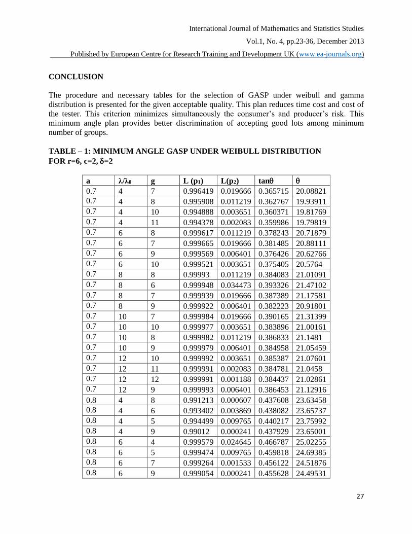
TABLE – 1: MINIMUM ANGLE GASP UNDER WEIBULL DISTRIBUTION

FOR r=6, c=2, =2

a λ/λ0 g L (p1) L(p2) tan

0.7 4 7 0.996419 0.019666 0.365715 20.08821

0.7 4 8 0.995908 0.011219 0.362767 19.93911

0.7 4 10 0.994888 0.003651 0.360371 19.81769

0.7 4 11 0.994378 0.002083 0.359986 19.79819

0.7 6 8 0.999617 0.011219 0.378243 20.71879

0.7 6 7 0.999665 0.019666 0.381485 20.88111

0.7 6 9 0.999569 0.006401 0.376426 20.62766

0.7 6 10 0.999521 0.003651 0.375405 20.5764

0.7 8 8 0.99993 0.011219 0.384083 21.01091

0.7 8 6 0.999948 0.034473 0.393326 21.47102

0.7 8 7 0.999939 0.019666 0.387389 21.17581

0.7 8 9 0.999922 0.006401 0.382223 20.91801

0.7 10 7 0.999984 0.019666 0.390165 21.31399

0.7 10 10 0.999977 0.003651 0.383896 21.00161

0.7 10 8 0.999982 0.011219 0.386833 21.1481

0.7 10 9 0.999979 0.006401 0.384958 21.05459

0.7 12 10 0.999992 0.003651 0.385387 21.07601

0.7 12 11 0.999991 0.002083 0.384781 21.0458

0.7 12 12 0.999991 0.001188 0.384437 21.02861

0.7 12 9 0.999993 0.006401 0.386453 21.12916

0.8 4 8 0.991213 0.000607 0.437608 23.63458

0.8 4 6 0.993402 0.003869 0.438082 23.65737

0.8 4 5 0.994499 0.009765 0.440217 23.75992

0.8 4 9 0.99012 0.000241 0.437929 23.65001

0.8 6 4 0.999579 0.024645 0.466787 25.02255

0.8 6 5 0.999474 0.009765 0.459818 24.69385

0.8 6 7 0.999264 0.001533 0.456122 24.51876

0.8 6 9 0.999054 0.000241 0.455628 24.49531





28

0.8 8 8 0.999846 0.000607 0.46311 24.84933

0.8 8 6 0.999884 0.003869 0.464609 24.91999

0.8 8 5 0.999904 0.009765 0.467366 25.04979

0.8 8 4 0.999923 0.024645 0.474487 25.38375

0.8 10 6 0.999969 0.003869 0.468154 25.08681

0.8 10 7 0.999964 0.001533 0.467061 25.03543

0.8 10 5 0.999974 0.009765 0.470939 25.21755

0.8 10 8 0.999959 0.000607 0.466631 25.01519

0.8 12 5 0.999991 0.009765 0.472895 25.30922

0.8 12 9 0.999984 0.000241 0.468393 25.09806

0.8 12 8 0.999986 0.000607 0.468564 25.1061

0.8 12 6 0.99999 0.003869 0.470097 25.17806

0.9 4 8 0.982936 0.000138 0.514565 27.22875

0.9 4 6 0.987174 0.000226 0.512466 27.13358

0.9 4 5 0.9893 0.000916 0.511721 27.09978

0.9 4 9 0.980823 0.000134 0.515668 27.27869

0.9 6 4 0.999163 0.003712 0.535328 28.16141

0.9 6 5 0.998953 0.000916 0.533941 28.0996

0.9 6 7 0.998535 0.000128 0.533705 28.08906

0.9 6 9 0.998117 0.000134 0.5339 28.09778

0.9 8 8 0.999691 0.000124 0.542741 28.49049

0.9 8 6 0.999768 0.000226 0.542814 28.49373

0.9 8 5 0.999807 0.000916 0.543168 28.5094

0.9 8 4 0.999845 0.003712 0.544671 28.57586

0.9 10 6 0.999938 0.000226 0.547232 28.6889

0.9 10 7 0.999928 0.000125 0.547145 28.68504

0.9 10 5 0.999948 0.000916 0.547605 28.70531

0.9 10 8 0.999918 0.000138 0.547127 28.68427

0.9 12 5 0.999983 0.000916 0.550046 28.81283

0.9 12 9 0.999969 0.000134 0.549552 28.79108

0.9 12 8 0.999972 0.000138 0.549556 28.79124

0.9 12 6 0.999979 0.000226 0.549669 28.79621

1.2 4 3 0.968982 0.000130 0.698697 34.94188

1.2 4 2 0.979213 0.000968 0.69206 34.68554

1.2 4 5 0.948839 0.000129 0.713507 35.50813

1.2 4 4 0.958858 0.000138 0.706053 35.22411

1.2 6 4 0.995597 0.000137 0.727064 36.01954

1.2 6 5 0.994499 0.000192 0.727866 36.04959

1.2 6 2 0.997796 0.000968 0.726165 35.98585

1.2 6 3 0.996696 0.000134 0.726283 35.99028





29

1.2 8 2 0.999581 0.000968 0.741853 36.56996

1.2 8 2 0.999581 0.000968 0.741853 36.56996

1.2 8 5 0.998953 0.000192 0.7416 36.56062

1.2 8 4 0.999163 0.000137 0.741445 36.55491

1.2 10 3 0.99983 0.000102 0.748925 36.83046

1.2 10 2 0.999887 0.000968 0.749586 36.85472

1.2 10 5 0.999717 0.000137 0.748987 36.83275

1.2 10 2 0.999887 0.000968 0.749586 36.85472

1.2 12 5 0.999904 0.000129 0.753195 36.98686

1.2 12 2 0.999961 0.000968 0.753881 37.01195

1.2 12 3 0.999942 0.000134 0.753188 36.98663

1.2 12 4 0.999923 0.000138 0.753181 36.98636

1.5 4 1 0.966827 0.001553 0.790879 38.33975

1.5 6 1 0.996129 0.001553 0.838562 39.9819

1.5 6 3 0.988433 0.000174 0.843774 40.15679

1.5 6 2 0.992274 0.000142 0.84051 40.04738

1.5 6 3 0.988433 0.000137 0.843774 40.15679

1.5 8 2 0.998476 0.000241 0.86137 40.74062

1.5 8 1 0.999238 0.001553 0.862051 40.76301

1.5 8 1 0.999238 0.001553 0.862051 40.76301

1.5 8 2 0.998476 0.000241 0.86137 40.74062

1.5 10 3 0.999372 0.000137 0.8729 41.11772

1.5 10 2 0.999581 0.000124 0.87272 41.11184

1.5 10 1 0.999791 0.001553 0.873892 41.14995

1.5 10 2 0.999581 0.000127 0.87272 41.11184

1.5 12 3 0.999784 0.000174 0.879287 41.32475

1.5 12 3 0.999784 0.000137 0.879287 41.32475

1.5 12 2 0.999856 0.000124 0.879226 41.32277

1.5 12 2 0.999856 0.000141 0.879226 41.32277





30

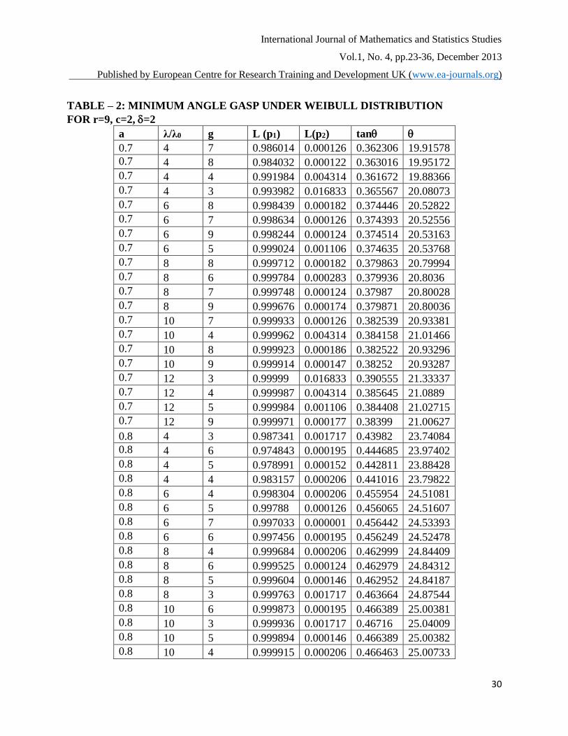
TABLE – 2: MINIMUM ANGLE GASP UNDER WEIBULL DISTRIBUTION

FOR r=9, c=2, =2


0.7 4 7 0.986014 0.000126 0.362306 19.91578

0.7 4 8 0.984032 0.000122 0.363016 19.95172

0.7 4 4 0.991984 0.004314 0.361672 19.88366

0.7 4 3 0.993982 0.016833 0.365567 20.08073

0.7 6 8 0.998439 0.000182 0.374446 20.52822

0.7 6 7 0.998634 0.000126 0.374393 20.52556

0.7 6 9 0.998244 0.000124 0.374514 20.53163

0.7 6 5 0.999024 0.001106 0.374635 20.53768

0.7 8 8 0.999712 0.000182 0.379863 20.79994

0.7 8 6 0.999784 0.000283 0.379936 20.8036

0.7 8 7 0.999748 0.000124 0.37987 20.80028

0.7 8 9 0.999676 0.000174 0.379871 20.80036

0.7 10 7 0.999933 0.000126 0.382539 20.93381

0.7 10 4 0.999962 0.004314 0.384158 21.01466

0.7 10 8 0.999923 0.000186 0.382522 20.93296

0.7 10 9 0.999914 0.000147 0.38252 20.93287

0.7 12 3 0.99999 0.016833 0.390555 21.33337

0.7 12 4 0.999987 0.004314 0.385645 21.0889

0.7 12 5 0.999984 0.001106 0.384408 21.02715

0.7 12 9 0.999971 0.000177 0.38399 21.00627

0.8 4 3 0.987341 0.001717 0.43982 23.74084

0.8 4 6 0.974843 0.000195 0.444685 23.97402

0.8 4 5 0.978991 0.000152 0.442811 23.88428

0.8 4 4 0.983157 0.000206 0.441016 23.79822

0.8 6 4 0.998304 0.000206 0.455954 24.51081

0.8 6 5 0.99788 0.000126 0.456065 24.51607

0.8 6 7 0.997033 0.000001 0.456442 24.53393

0.8 6 6 0.997456 0.000195 0.456249 24.52478

0.8 8 4 0.999684 0.000206 0.462999 24.84409

0.8 8 6 0.999525 0.000124 0.462979 24.84312

0.8 8 5 0.999604 0.000146 0.462952 24.84187

0.8 8 3 0.999763 0.001717 0.463664 24.87544

0.8 10 6 0.999873 0.000195 0.466389 25.00381

0.8 10 3 0.999936 0.001717 0.46716 25.04009

0.8 10 5 0.999894 0.000146 0.466389 25.00382

0.8 10 4 0.999915 0.000206 0.466463 25.00733





31

0.8 12 5 0.999964 0.000126 0.468301 25.09376

0.8 12 3 0.999978 0.001717 0.469089 25.13073

0.8 12 2 0.999986 0.014339 0.475092 25.41202

0.8 12 6 0.999957 0.000195 0.468295 25.09344

0.9 4 4 0.968108 0.000171 0.522441 27.58441

0.9 4 2 0.983925 0.002171 0.515177 27.25649

0.9 4 3 0.975985 0.000101 0.518276 27.39663

0.9 6 4 0.996658 0.000171 0.534683 28.13264

0.9 6 3 0.997493 0.000101 0.534287 28.11501

0.9 6 5 0.995824 0.000001 0.535128 28.15249

0.9 6 2 0.998328 0.002171 0.534949 28.14453

0.9 8 3 0.999526 0.000101 0.542877 28.49654

0.9 8 2 0.999684 0.002171 0.543918 28.54258

0.9 8 5 0.999211 0.00001 0.542999 28.50193

0.9 8 4 0.999369 0.000171 0.542911 28.49801

0.9 10 4 0.99983 0.000176 0.54717 28.68617

0.9 10 3 0.999872 0.000101 0.5472 28.68747

0.9 10 2 0.999915 0.002171 0.548312 28.73648

0.9 10 5 0.999787 0.00001 0.547196 28.68732

0.9 12 4 0.999942 0.000171 0.549567 28.79175

0.9 12 3 0.999957 0.000101 0.549612 28.79373

0.9 12 2 0.999971 0.002171 0.550745 28.84353

0.9 12 5 0.999928 0.00001 0.549578 28.79222

1.2 4 1 0.963939 0.000001 0.702331 35.08156

1.2 6 1 0.995762 0.000949 0.727636 36.04097

1.2 6 3 0.987341 0.0001 0.733217 36.24949

1.2 6 2 0.991543 0.000101 0.730036 36.1308

1.2 8 2 0.998328 0.000101 0.742065 36.57782

1.2 8 1 0.999163 0.000949 0.742149 36.58091

1.2 8 3 0.997493 0.0001 0.74276 36.60349

1.2 10 1 0.99977 0.000949 0.749659 36.85741

1.2 10 2 0.99954 0.000124 0.749121 36.83765

1.2 10 3 0.99931 0.00001 0.7493 36.84422

1.2 12 1 0.999921 0.000949 0.753897 37.01254

1.2 12 2 0.999842 0.000127 0.753242 36.98859

1.2 12 3 0.999763 0.0001 0.753376 36.9935

1.5 6 1 0.985834 0.000129 0.846002 40.23127

1.5 6 2 0.97187 0.000001 0.858155 40.63471

1.5 8 1 0.99704 0.000129 0.862613 40.78147

1.5 8 2 0.994088 0.000001 0.865171 40.86542





32

1.5 10 1 0.999163 0.000145 0.873086 41.12376

1.5 10 2 0.998328 0.00001 0.873822 41.14768

1.5 12 1 0.999708 0.000126 0.879358 41.32703

1.5 12 2 0.999416 0.000001 0.879611 41.33523

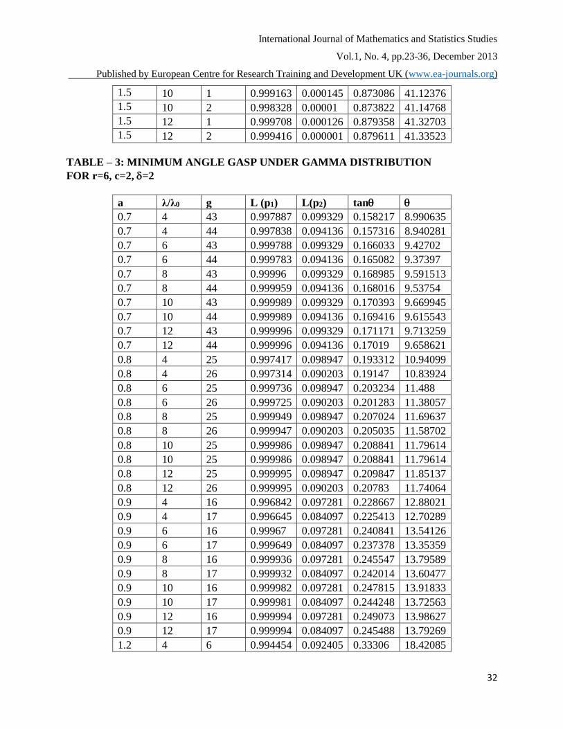
TABLE – 3: MINIMUM ANGLE GASP UNDER GAMMA DISTRIBUTION

FOR r=6, c=2, =2


0.7 4 43 0.997887 0.099329 0.158217 8.990635

0.7 4 44 0.997838 0.094136 0.157316 8.940281

0.7 6 43 0.999788 0.099329 0.166033 9.42702

0.7 6 44 0.999783 0.094136 0.165082 9.37397

0.7 8 43 0.99996 0.099329 0.168985 9.591513

0.7 8 44 0.999959 0.094136 0.168016 9.53754

0.7 10 43 0.999989 0.099329 0.170393 9.669945

0.7 10 44 0.999989 0.094136 0.169416 9.615543

0.7 12 43 0.999996 0.099329 0.171171 9.713259

0.7 12 44 0.999996 0.094136 0.17019 9.658621

0.8 4 25 0.997417 0.098947 0.193312 10.94099

0.8 4 26 0.997314 0.090203 0.19147 10.83924

0.8 6 25 0.999736 0.098947 0.203234 11.488

0.8 6 26 0.999725 0.090203 0.201283 11.38057

0.8 8 25 0.999949 0.098947 0.207024 11.69637

0.8 8 26 0.999947 0.090203 0.205035 11.58702

0.8 10 25 0.999986 0.098947 0.208841 11.79614

0.8 10 25 0.999986 0.098947 0.208841 11.79614

0.8 12 25 0.999995 0.098947 0.209847 11.85137

0.8 12 26 0.999995 0.090203 0.20783 11.74064

0.9 4 16 0.996842 0.097281 0.228667 12.88021

0.9 4 17 0.996645 0.084097 0.225413 12.70289

0.9 6 16 0.99967 0.097281 0.240841 13.54126

0.9 6 17 0.999649 0.084097 0.237378 13.35359

0.9 8 16 0.999936 0.097281 0.245547 13.79589

0.9 8 17 0.999932 0.084097 0.242014 13.60477

0.9 10 16 0.999982 0.097281 0.247815 13.91833

0.9 10 17 0.999981 0.084097 0.244248 13.72563

0.9 12 16 0.999994 0.097281 0.249073 13.98627

0.9 12 17 0.999994 0.084097 0.245488 13.79269

1.2 4 6 0.994454 0.092405 0.33306 18.42085





33

1.2 4 7 0.993532 0.062131 0.322564 17.87783

1.2 6 6 0.99938 0.092405 0.352655 19.42548

1.2 6 7 0.999276 0.062131 0.341302 18.84488

1.2 8 6 0.999876 0.092405 0.360548 19.82666

1.2 8 7 0.999855 0.062131 0.348916 19.23469

1.2 10 6 0.999965 0.092405 0.364409 20.02222

1.2 10 7 0.999959 0.062131 0.352648 19.42512

1.2 12 6 0.999988 0.092405 0.366571 20.13148

1.2 12 7 0.999986 0.062131 0.354739 19.5316

1.5 4 3 0.991235 0.095692 0.43236 23.38174

1.5 4 4 0.988331 0.043769 0.409923 22.28984

1.5 6 3 0.998949 0.095692 0.460196 24.71172

1.5 6 4 0.998599 0.043769 0.43534 23.52542

1.5 8 3 0.999783 0.095692 0.471907 25.26294

1.5 8 4 0.999711 0.043769 0.44631 24.0517

1.5 10 3 0.999938 0.095692 0.477734 25.53538

1.5 10 4 0.999917 0.043769 0.451801 24.3135

1.5 12 3 0.999978 0.095692 0.481024 25.68869

1.5 12 4 0.999971 0.043769 0.454908 24.46116

1.8 4 2 0.985622 0.076674 0.507976 26.92949

1.8 4 3 0.97851 0.021231 0.48233 25.74939

1.8 6 2 0.998148 0.076674 0.542855 28.49555

1.8 6 3 0.997223 0.021231 0.512532 27.13658

1.8 8 2 0.999605 0.076674 0.558379 29.17809

1.8 8 3 0.999407 0.021231 0.526843 27.7822

1.8 10 2 0.999885 0.076674 0.566265 29.52136

1.8 10 3 0.999827 0.021231 0.534216 28.11186

1.8 12 2 0.999959 0.076674 0.570764 29.71615

1.8 12 3 0.999938 0.021231 0.538442 28.2999





34

TABLE – 4: MINIMUM ANGLE GASP UNDER GAMMA DISTRIBUTION

FOR r=9, c=2, =2


0.7 4 14 0.997199 0.097019 0.157932 8.974696

0.7 4 15 0.996999 0.082128 0.155396 8.832866

0.7 6 14 0.999714 0.097019 0.165622 9.404079

0.7 6 15 0.999694 0.082128 0.162938 9.254326

0.7 8 14 0.999945 0.097019 0.168555 9.567573

0.7 8 15 0.999942 0.082128 0.165821 9.415183

0.7 10 14 0.999985 0.097019 0.169958 9.645709

0.7 10 15 0.999984 0.082128 0.167201 9.492098

0.7 12 14 0.999995 0.097019 0.170734 9.688892

0.7 12 15 0.999995 0.082128 0.167964 9.534614

0.8 4 9 0.996248 0.085758 0.19076 10.79997

0.8 4 10 0.995832 0.065276 0.186646 10.57239

0.8 6 9 0.999607 0.085758 0.20033 11.32809

0.8 6 10 0.999564 0.065276 0.195947 11.08647

0.8 8 9 0.999924 0.085758 0.204043 11.53249

0.8 8 10 0.999916 0.065276 0.199573 11.28641

0.8 10 9 0.999979 0.000001 0.188178 10.65716

0.8 10 10 0.999977 0.065276 0.201319 11.38261

0.8 12 9 0.999993 0.085758 0.20682 11.68516

0.8 12 10 0.999992 0.065276 0.202288 11.43593

0.9 4 6 0.995267 0.085293 0.22605 12.73765

0.9 4 7 0.99448 0.056589 0.219322 12.37035

0.9 6 6 0.999491 0.085293 0.237729 13.37266

0.9 6 7 0.999407 0.056589 0.230513 12.98068

0.9 8 6 0.999901 0.085293 0.242339 13.62236

0.9 8 7 0.999884 0.000001 0.221671 12.49869

0.9 10 6 0.999972 0.085293 0.244569 13.74302

0.9 10 7 0.999968 0.056589 0.237129 13.3401

0.9 12 6 0.99999 0.085293 0.24581 13.81008

0.9 12 7 0.999989 0.056589 0.238331 13.40531

1.2 4 4 0.98576 0.018202 0.31051 17.2501

1.2 4 5 0.982231 0.006686 0.307968 17.11714

1.2 6 4 0.998331 0.018202 0.326334 18.07329

1.2 6 5 0.997914 0.006686 0.32268 17.88386

1.2 8 4 0.999661 0.018202 0.333368 18.43674

1.2 8 5 0.999576 0.006686 0.32953 18.23859





35

1.2 8 4 0.999661 0.018202 0.333368 18.43674

1.2 10 5 0.99988 0.006686 0.33299 18.41724

1.2 10 4 0.999904 0.018202 0.336888 18.61806

1.2 12 4 0.999966 0.018202 0.338874 18.72016

1.2 12 5 0.999958 0.006686 0.334947 18.51814

1.5 4 2 0.978393 0.025869 0.406496 22.12154

1.5 4 3 0.967766 0.004161 0.401822 21.89132

1.5 6 2 0.997229 0.025869 0.427931 23.1676

1.5 6 3 0.995847 0.004161 0.41916 22.7415

1.5 8 2 0.999414 0.025869 0.43824 23.66497

1.5 8 3 0.999121 0.00001 0.427026 23.12376

1.5 10 2 0.99983 0.025869 0.443538 23.91909

1.5 10 3 0.999746 0.004161 0.433904 23.45624

1.5 12 2 0.99994 0.025869 0.446563 24.06375

1.5 12 3 0.999909 0.004161 0.436841 23.59767

1.8 6 1 0.996421 0.058417 0.533289 28.0705

1.8 6 2 0.992854 0.003413 0.505565 26.81955

1.8 8 1 0.99921 0.058417 0.547778 28.71296

1.8 8 2 0.99842 0.003413 0.517931 27.38106

1.8 10 1 0.999766 0.058417 0.555354 29.04579

1.8 10 2 0.999532 0.003413 0.524819 27.69133

1.8 12 1 0.999915 0.058417 0.559722 29.2367

1.8 12 2 0.99983 0.003413 0.528872 27.8731

REFERENCES:

R. R. L. Kantam, K. Rosaiah and G. S. Rao (2001), Acceptance sampling plans from truncated

life tests based on the Birnbaum-saunders distribution for Percentilies, Communications

in Statistics – Simulation and Computation, 39, 119 – 136.

A. Baklizi (2003). Acceptance sampling based on truncated life tests in the Pareto distribution of

the second kind, Advances and Applications in statistics, 3, 33-48.

N. Balakrishnan, V. Leiva and J. Lopez (2007). Acceptance sampling plans from truncated life

tests based on the generalized Birnbaum-Saunders distribution, Communications in

Statistics - Simulation and Computation, 36, 643-656.

Y. L. Lio, T. R. Tsai and S. J Wu (2010). Acceptance sampling plans from truncated life tests

based on the

Birnbaum-Saunders distribution for Percentiles, Communications in Statistics – Simulation and

Computation, 39, 119-136.

Y.L. Lio, T – R. Tsai and S – J. Wu (2010). Acceptance sampling plans from truncated life tests

based on Burr type XII percentiles, Journal fo the Chinese institute of Industrial

Engineers, 27, 270 – 280.





36

R.D. Gupta and D. Kundu, Generalized exponential distribution: existing methods and recent

developments, J. Statistics, Plannnnnning Inference 137 (2007) pp. 3537 – 3547.

G. Srinivasa Rao, (2009), A Group Acceptance Sampling Plans for Lifetimes .Following a

Generalized Exponential Distribution. 1, 75 – 85.

Bush N. Leonard E.J., and Merchant M.Q.M.Jr.,(1953) A Method of Single and Double Sampling

OC curves Utilizing the Tangent of the Point of the Inflexion, (ENASR), No, PR-7, 1-

77.


Documents

DESINGNING GROUP ACCEPTANCE SAMPLING … · DESIGNING GROUP ACCEPTANCE SAMPLING PLANS FORTHE WEIBULL AND GAMMA DISTRIBUTION USING MINIMUM ANGLE METHOD Dr. A. R. Sudamani Ramaswamy