Designing verbal autopsy studies - Gary King - Harvard University

RESEARCH Open Access

Designing verbal autopsy studiesGary King1*, Ying Lu2, Kenji Shibuya3

Abstract

Background: Verbal autopsy analyses are widely used for estimating cause-specific mortality rates (CSMR) in thevast majority of the world without high-quality medical death registration. Verbal autopsies – survey interviewswith the caretakers of imminent decedents – stand in for medical examinations or physical autopsies, which areinfeasible or culturally prohibited.

Methods and Findings: We introduce methods, simulations, and interpretations that can improve the design ofautomated, data-derived estimates of CSMRs, building on a new approach by King and Lu (2008). Our resultsgenerate advice for choosing symptom questions and sample sizes that is easier to satisfy than existing practices.For example, most prior effort has been devoted to searching for symptoms with high sensitivity and specificity,which has rarely if ever succeeded with multiple causes of death. In contrast, our approach makes this searchirrelevant because it can produce unbiased estimates even with symptoms that have very low sensitivity andspecificity. In addition, the new method is optimized for survey questions caretakers can easily answer rather thanquestions physicians would ask themselves. We also offer an automated method of weeding out biased symptomquestions and advice on how to choose the number of causes of death, symptom questions to ask, andobservations to collect, among others.

Conclusions: With the advice offered here, researchers should be able to design verbal autopsy surveys andconduct analyses with greatly reduced statistical biases and research costs.

IntroductionEstimates of cause-specific morality rates (CSMRs) areurgently needed for many research and public policygoals, but high quality death registration data exists inonly 23 of 192 countries [1]. Indeed, more than two-thirds of deaths worldwide occur without any medicaldeath certification [2]. In response, researchers areincreasingly turning to verbal autopsy analyses, a techni-que “growing in importance” [3]. Verbal autopsy studiesare now widely used in the developing world to estimateCSMRs, disease surveillance, and sample registration[4-6], as well as risk factors, infectious disease outbreaks,and the effects of public health interventions [7-9].The idea of verbal autopsy analyses is to ask (usually

around 10-100) questions about symptoms (includingsome signs and other indicators) of the caretakers ofrandomly selected decedents and to infer from theanswers the cause of death. Three approaches have beenused to draw these inferences. We focus on the fourth

and newest approach, by King and Lu, which requiresmany fewer assumptions [10]. We begin by summarizingthe main existing approaches. We then discuss our maincontribution, which is in the radical new (and mucheasier) ways of writing symptom questions, weeding outbiased symptoms empirically, and choosing valid samplesizes.The first is physician review, where a panel of (usually

three) physicians study the reported symptoms andassign each death to a cause, and then researchers totalup the CSMR estimates [11]. This method tends to beexpensive, time- consuming, unreliable (in the sensethat physicians disagree over a disturbingly large percen-tage of the deaths), and incomparable across populations(due to differing views of local physicians); in addition,the reported performance of this approach is often exag-gerated by including information from medical recordsand death certificates among the symptom questions,which is unavailable in real applications [12]. The sec-ond approach is expert systems, where a decision tree isconstructed by hand to formalize the best physicians’* Correspondence: [email protected]

1Institute for Quantitative Social Science, Harvard University, Cambridge MA02138, USA

King et al. Population Health Metrics 2010, 8:19http://www.pophealthmetrics.com/content/8/1/19

© 2010 King et al; licensee BioMed Central Ltd. This is an Open Access article distributed under the terms of the Creative CommonsAttribution License (http://creativecommons.org/licenses/by/2.0), which permits unrestricted use, distribution, and reproduction inany medium, provided the original work is properly cited.

mailto:[email protected]

http://creativecommons.org/licenses/by/2.0

judgments. The result is reliable but can be highly inac-curate with symptoms measured with error [13,14].The third approach is statistical classification and

requires an additional sample of deaths from a medicalfacility where each cause is known and symptoms arecollected from relatives. Then a parametric statisticalclassification method (e.g., multinomial logit, neural net-works, or support vector machines) is trained on thehospital data and used to predict the cause of eachdeath in the community [15]. These methods areunbiased only if one of two conditions hold. The first isthat the symptoms have 100% sensitivity and specificity.This rarely holds because of the inevitable measurementerror in survey questions and the fact that symptomsresult from rather than (as the predictive methodsassume) generate the causes that lead to death. A sec-ond condition is that the symptoms represent all predic-tive information and also that everything aboutsymptoms and the cause of death is the same in thehospital and community (technically, the symptomsspan the space all predictors of the cause of death andthe joint distribution of causes and symptoms are thesame in both samples [16]). This condition is also highlyunlikely to be satisfied in practice.Like statistical classification, the King-Lu method [10]

is data-derived and so requires less qualitative judgment;it also requires hospital and community samples, butmakes the much less restrictive assumption that onlythe distribution of symptoms for a given cause of deathis the same in the hospital and community. That is,when diseases present to relatives or caregivers in simi-lar ways in the hospital and community, then themethod will give accurate estimates of the CSMR. Thisis true even when the symptom questions chosen havevery low (but nonzero) sensitivity and specificity, whenthese questions have random measurement error, whenthe prevalence of different symptoms and the CSMR dif-fer dramatically between the hospital and community, orif the data from the hospital are selected via case-controlmethods. Case-control selection, where the same num-ber of deaths are selected in the hospital for each cause,can save considerable resources in conducting the sur-vey, especially in the presence of rare causes of death inthe community. The analysis (with open source and freesoftware) is easy and can be run on standard desktopcomputers. In addition, so long as the symptoms thatoccur with each cause of death do not change dramati-cally over time (even if the prevalence of different causesdo change), the hospital sample can be built up overtime, further reducing the costs.Conceptually, the King-Lu method involves four main

advances (see Appendix A for a technical summary).First, King-Lu estimates the CSMR, which is the mainquantity of interest in the field, rather than the correct

classification of any individual death. The method gener-ates unbiased estimates of the CSMR even when thepercent of individual deaths that can be accurately clas-sified is very low. (The method also offers a better wayto classify individual deaths, when that is of interest; seeAppendix A and [[10], Section 8].) Second is a generali-zation to multiple causes of the standard “back calcula-tion” epidemiological correction for estimating theCSMR with less than perfect sensitivity and specificity[17,18]. The third switches “causes” and “effects” and soit properly treats the symptoms as consequences ratherthan causes of the injuries and diseases that lead todeath. Since symptoms are now the outcome variables,it easily accommodates random measurement error insurvey responses. The final advance of this method isdropping all parametric modeling assumptions andswitching to a fully nonparametric approach. The resultis that we merely need to tabulate the prevalence of dif-ferent symptom profiles in the community and the pre-valence of different symptom profiles for each cause ofdeath in the hospital. No modeling assumptions, notmuch statistical expertise, and very little tweaking andtesting are required to use the method.Building on [10], we now develop methods that mini-

mize statistical bias in Section and inefficiency in Sec-tion 0.4 by appropriately choosing symptom questions,defining causes of death, deciding how many interviewsto conduct in the hospital and community, and adjust-ing for known differences between samples. Software toestimate this model is available at http://gking.harvard.edu/va.

Avoiding Bias[10] indicates how to avoid bias from a statistical per-spective. Here, we turn these results and our extensionsof them into specific, practical suggestions for choosingsurvey questions. We do this first via specific adviceabout designing questions (Section 0.1), then in a sec-tion that demonstrates the near irrelevance of sensitivityand specificity, which most previous analyses havefocused on (Section 0.2), and finally via a specificmethod that automates the process of weeding outquestions that violate our key assumption (Section 0.3).

0.1 Question ChoiceThe key to avoiding bias is ensuring that patients whodie in a hospital present their symptoms in the verbalautopsy survey instrument (as recorded by relatives andcaregivers) in the same way as do those in the commu-nity (or in other words that the assumption in Equation3 holds). As such, it may seem like the analyst is at themercy of the real world: either diseases present thesame way in the two locations or they do not. In fact,this is not the case, as the analyst has in the choice of


Page 2 of 12

http://gking.harvard.edu/va


symptom questions a powerful tool to reduce bias. Inother words, how the patient presents symptoms to rela-tives and caregivers is only relevant inasmuch as theanalyst asks about them. That means that avoiding biasonly requires not posing symptom questions likely toappear different to those in the two samples (amongthose who cared for people dying of the same cause).For an example of a violation of this assumption, con-

sider that relatives of those who died in a medical facil-ity would be much more likely than their counterpartsin the community to know if the patient under theircare suffered from high blood pressure or anemia, sincerelatives could more easily learn these facts only frommedical personnel in a hospital than in the communitywithout proper ways of measuring these quantities.Avoiding questions like these can greatly increase theaccuracy of estimates. In contrast, the respondent notingwhether they observed the patient bleeding from thenose would be unlikely to be affected by a visit to a hos-pital, even under instruction from medical personnel.This fundamental point suggests avoiding any symp-

tom questions about concepts more likely to be knownby physicians and shared with patients or taught tocaregivers than known by those in the community whowere unlikely to have been in contact with medical per-sonnel. We should therefore be wary of more sophisti-cated, complicated, or specialized questions likely to beanswerable only by those who have learned them frommedical personnel. The questions a relative is even likelyto understand and answer accurately are not thosewhich a physician might determine from a direct physi-cal examination. Trying to approximate the questionsphysicians ask themselves is thus likely to lead to bias. Incontrast, finding questions respondents are easily able toanswer, and likely to give the same answers despite theirexperience in a medical facility, is best.It is important to understand how substantially differ-

ent these recommendations are from the way most havegone about selecting verbal autopsy survey questions.Most studies now choose questions intended to havethe highest possible sensitivity and specificity. At best,this emphasis does not help much, because they are notrequired for accurate CSMR inferences, a point wedemonstrate in the next section. However, this emphasiscan also lead to huge biases when symptom questionswith highest sensitivity and specificity are those that areclosest to questions physicians would ask themselves,medical tests, or other facts which relatives of thedeceased learn about about when in contact with medi-cal personnel. (A related practical suggestion for redu-cing bias is to select a hospital as similar as possible tothe community population. In most cases, physicalproximity to large portions of the community will behelpful, but the main goal should be selecting a medical

facility which has patients that present their symptomsin similar ways in hospital as in the community for eachcause of death.)

0.2 The Near Irrelevance of Sensitivity and SpecificityVerbal autopsy researchers regularly emphasize selectingsymptom questions based on their degree of sensitivityand specificity. It is hard to identify a study that hasselected symptom questions in any other way, and manycriticize verbal autopsy instruments for their low or vari-able levels of sensitivity and specificity across data setsand countries. This emphasis may be appropriate forapproaches that use statistical classification methods, asthey require 100% sensitivity and specificity, but suchstringent and unachievable requirements are not neededwith the King-Lu approach. We now provide evidenceof this result.We begin by generating data sets with 3,000 sampled

deaths in the community and the same number in anearby hospital (our conclusions do not depend on thesample size). The data consist of answers to 50 symp-tom questions – which we use in subsets of 20, 30, and50 – and 10 causes of death. Because we generated thedata, we know both the answers to the symptom ques-tions and the cause of death for everyone in both sam-ples; however, we set aside the causes of death for thosein the community, which we ordinarily would not know,and use them only for evaluation after running eachanalysis.We first generate a “high sensitivity” symptom, which

we shall study the effect of. It has 100% sensitivity forthe first cause of death and 0% for predicting any othercause of death (i.e., it also has high specificity). (Theprevalence of this first cause of death is 20% overall.)Every other symptom has a maximum of 30% sensitivityfor any cause of death. For each of 20, 30, and 50 symp-toms, we generate 80 data sets with and without thishigh sensitivity symptom (each with 3,000 samples fromthe hospital and 3,000 from the community). In eachdata set, we estimate the CSMR. We then average overthe 80 results for each combination of symptoms andcompare the average of these estimates to the truth.This averaging is the standard way of setting aside thenatural sampling variability and focusing on systematicpatterns.The results appear in Table 1, with different numbers

of symptoms given in separate columns. The first tworows of the table give the difference in the proportion ofdeaths estimated to be in the first category with (for thefirst row) and without (for the second) the high sensitiv-ity symptom. Clearly the difference between the num-bers in the first two rows is trivial, indicating the nearirrelevance of including this symptom. The second pairof rows in the table give the absolute error in estimating


Page 3 of 12

the effects for all causes of death. Again, the resultsshow the irrelevance of including this high sensitivitysymptom. (The numbers in the tables are proportions,so that 0.0128 represents a 1.28 percentage point differ-ence between the estimate and the truth.)Searching for high sensitivity symptoms is thus at best

a waste of time. The essential statistical reason for thisis that symptoms do not cause the diseases and injuriesthat result in death. Instead, the symptoms are conse-quences of these diseases and injuries. As such, asses-sing whether the symptoms have high sensitivity andspecificity for predicting something they do not predict(or cause) in the real world, and are not needed to pre-dict with the method, is indeed irrelevant.The King-Lu method works by appropriately treating

symptoms as consequences of the disease or injury thatcaused death. Even if they were available, having symp-toms that approximate highly predictive bioassays isneither necessary nor even very helpful. Any symptomwhich is a consequence of one or more of the causes ofdeath can be used to improve CSMR estimates, even ifit has random measurement error. So long as a symp-tom has some, possibly low-level, relationship to thecauses of death, it can be productively used. Even appar-ently tertiary, behavioral, or non-medical symptoms thathappen to be consequences of the illness can be used solong as they are likely to be reported in the same wayregardless of whether the death occurred in a hospitalor the community.

0.3 Detecting Biased Symptom QuestionsSuppose we follow the advice offered on selecting symp-tom questions in Section 0.1, but we make a mistakeand include a question which unbeknownst to usinduces bias. An example would be a symptom which,for a given cause of death, is overreported in the hospi-tal vs the community. Appendix B shows that in somecircumstances it’s possible to detect this biased symp-tom question, in which case we can remove it and rerunthe analysis without the offending question. Since many

verbal autopsy instruments include a large number ofquestions, this procedure could be used to eliminatequestions without much cost. In this section, we presentanalyses in simulated and real data that demonstrate theeffectiveness of this simple procedure.We thus conduct a simulations where different num-

bers of symptom questions are “misreported” – that is,reported with different frequencies in the hospital andcommunity samples for given causes of death. We gen-erate two sets of data, one with 3,000 deaths in each ofthe hospital and community samples and the other with500 deaths in each; both have 10 different causes ofdeath, with distribution D = (0.2, 0.2, 0.2, 0.1, 0.05, 0.05,0.05, 0.05, 0.05, 0.05). The CSMF distribution of D inthe hospital is uniform (0.1 for each cause) and in thecommunity is D = (0.2, 0.2,..., 0.2, 0.05). Table 2 sum-marizes the pattern of misreporting we chose. In thistable, the first row indicates which symptom number isto be set up as misreported when applicable. The sec-ond row gives the extent of the violation of the keyassumption of the King-Lu method (in Equation 3) –the percentage point difference between the symptom’smarginal distribution in the community and hospitalsamples. For example, where three symptoms are misre-ported, we generate data using the first three columnsof Table 2 and so the marginal prevalence of the first,fifth, and 10th symptoms in the community sample areset to be different from the hospital according to thefirst three elements of the second column. When fivesymptoms are misreported, the distribution of the first,fifth, 10th, 11th and 15th symptoms will be set to be dif-ferent in the degree as indicated, etc.We first give our large sample and small sample

results and then give a graphic illustration of the bias-efficiency trade-offs involved in symptom selection.Larger Sample SizeFor the large (n = 3, 000) simulation, Table 3 sum-marizes the results of symptom selection for each differ-ent simulation. The first two columns indicate,respectively, the total number of symptoms and thenumber of biased symptoms included in the communitysample. The third column indicates the number ofsymptoms flagged (at the 5% significance level), usingthe selection procedure proposed in Appendix B. Thefinal column indicates the number of biased symptomsthat are correctly identified.Table 3 indicates that our symptom selection proce-

dure is highly accurate. Except the first simulation,which has disproportionately many misreported

Table 1 Absolute error rates with and without asymptom that has very high sensitivity for the first causeof death

Number of Symptoms

20 30 50

Absolute Error for First Cause of Death

With high sensitivity symptom 0.0128 0.0120 0.0123

Without high sensitivity symptom 0.0128 0.0124 0.0124

Mean Absolute Error

With high sensitivity symptom 0.0090 0.0081 0.0084

Without high sensitivity symptom 0.0092 0.0082 0.0085

The first and second row of each pair are very similar, which illustrates theirrelevance of finding symptoms with high sensitivity.

Table 2 List of Misreported Symptoms

Symptom 1 5 10 11 15 20 21 25 30 31

Misreport 30% -30% -50% 30% -30% 30% -30% -50% 30% -30%


Page 4 of 12

symptoms (three out of 10), our proposed method cor-rectly selects nearly all the biased symptoms. There isonly one false positive case, but if we were to changethe joint significance level to 0.01, this symptom wouldno longer being incorrectly selected.Smaller Sample SizeOur smaller (n = 500) simulation necessarily results inlarger CSMR variances. This, in turn, affects the powerof the method described in Appendix B to detect biasedsymptoms. And at the same time it makes it more costlyto discard unbiased symptoms. As shown in Table 4, wemiss some symptoms at the 5% level. If we relax thetype I error rate to 10%, more biased symptoms aredetected. The table also conveys the additional variationin our methods due to the smaller sample size.Bias-Efficiency Trade-offsAlthough these results are encouraging, in real-worlddata, a trade-off always exists between choosing a lowersignificance level to ensure that all biased symptoms areselected at a cost of increasing the false positive rate, vs.choosing a higher significance level to reduce the falsepositive rate at the cost of missing some biased symp-toms. In this section, we illustrate how different samplesizes can affect the decision about the significance levelin practice.We now choose “large” (3, 000), “medium” (1, 000),

and “small” (500) samples for each of the community

and hospital samples. In each, 10 of 50 symptoms arebiased. We then successively remove symptoms all theway up to the 50% signficance level criterion (to see thefull consequence of dropping too many symptoms).Figure 1 gives the results in a graph for each samplesize separately, (large, medium, and small sample sizesfrom left to right). Each graph then displays the meansquare error (MSE) between the true and estimatedcause-of-death distribution for each run of the modelvertically, removing more and more symptoms as fromthe left to the right along the horizontal axis of eachgraph. (In real applications, we would never be able tocompute the MSE, because we do not observe the truecause of death, but we can do it here for validationbecause the data are simulated.) That is, all symptomsare included for the first point on the left, and eachsubsequent point represents a model estimated with anadditional symptom dropped, as selected by our proce-dure. Circles are plotted for models where a biasedsymptom was selected and solid disks are plotted forunbiased symptoms.Three key results can be seen in this figure. First, for

all three sample sizes and corresponding graphs, allbiased symptoms are selected before any unbiasedsymptoms are selected, without a single false positive(which can be seen because all circles appear to the leftof all solid disks).Second, all three figures are distinctly U-shaped. The

reason can be seen beginning at the left of each graphwith a sample that includes biased symptoms. As ourselection procedure detects and deletes these biasedsymptoms one at a time, the MSE drops due to thereduction in bias of the estimate of the CSMR. Drop-ping additional symptoms after all biased ones aredropped, which can occur if the wrong significance levelis chosen, will induce no bias in our results but canreduce efficiency. If few unbiased symptoms are deleted,little harm is done since most verbal autopsy data setshave many symptoms and so enough efficiency to coverthe loss. However, if many more unbiased symptoms aredropped, the MSE starts to increase because of ineffi-ciency, which explains the rest of the U-shape.Finally, in addition to choosing the order in which

symptoms should be dropped, our automated selectionprocedure also suggests a stopping rule based on theuser-choice of a significance level. The 5% and 10% sig-nificance level stopping rules appear on the graphs assolid and dashed lines. These do not appear exactly atthe bottom of the U-shape, cleanly distinguishing biasedfrom unbiased symptoms, but for all three sample sizesthe results are very good. In all cases, using this stop-ping rule would greatly improve the MSE of the ulti-mate estimator. Our procedure thus seems to do workreasonably well.

Table 3 Performance of the Symptom Selection Methodwith n = 3, 000

symptoms biased flagged correct

10 3 0 0

20 3 3 3

30 3 3 3

50 3 3 3

20 5 5 5

30 5 5 5

50 5 6 5

50 10 10 10

Table 4 Performance of the Symptom Selection Methodwith n = 500

5% error rate 10% error rate

symptoms biased flagged correct flagged correct

10 3 0 0 1 1

20 3 3 3 3 3

30 3 2 2 5 3

50 3 3 3 5 3

20 5 2 2 3 3

30 5 3 3 4 4

50 5 4 4 4 4

50 10 6 3 6 3


Page 5 of 12

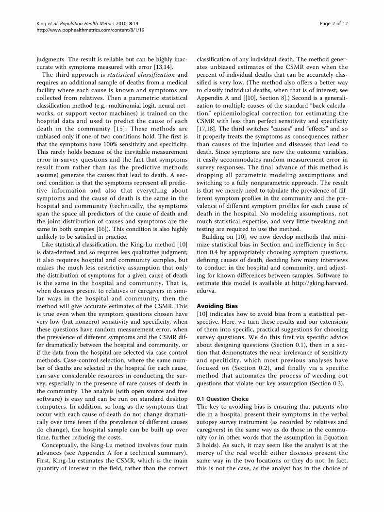
Empirical Evidence from TanzaniaFinally, we apply the proposed validation method to areal data example where we happen to observe the truecauses of death in both samples [19]. These data fromTanzania have 12 causes of death and 51 symptomsquestions but a small sample of only 282 deaths in thecommunity sample and 1,261 in the hospital. Applyingour symptom selection method, at the 5% level, foursymptoms would be deleted, which in fact correspondsto the smallest MSE along the iterative model selectionprocess. Figure 2 gives these results.To illustrate this example in more details, Table 5 shows

how the mean square error changes when specific symp-toms were sequentially selected, And in Table 6 we present

the change in each cause-specific mortality fraction esti-mate as these four symptoms are sequentially removed.The first three symptoms which were sequentially

dropped – fever, pale, and confused – are so non-speci-fic that they were almost unable to distinguish all of the12 causes clinically, with the possible exception ofdeaths from injuries. Although high levels of specificityare not necessary for our method, we do require that itis above zero. Wheezing is a distinctive clinical symp-tom of an airway obstruction, typically observed inpatients with asthma or bronchitis, and would be usefulto identify deaths from such causes. However, ourmethod suggests that it was highly biased. In fact,

Figure 1 For sample sizes of 3,000 (left graph), 1,000 (middle), and 500 (right), the figure gives the mean square error as symptomsare removed using our detection diagnostic. The mean square error first declines, as bad symptoms are removed and bias drops, and thenincreases, as unbiased symptoms are dropped and variance increases. The procedure selects all biased symptoms (open circles) before unbiasedsymptoms (solid disks). The vertical line indicates where our automated procedure would indicate that we should stop.

Figure 2 Validation of Mean Square Error in Tanzania, wherethe true cause of death is known in both samples.

Table 5 List of symptoms that are sequentially removedfrom the analysis

prevalence

symptoms hospital community mean square error

- - - 0.0016

fever 72.6 45.4 0.0013

pale 33.1 17.4 0.0018

confused 30.8 14.5 0.0012

wheezing 8.3 21.3 0.0012

vomit 49.0 35.5 0.0015

difficult-swallow 18.9 7.4 0.0015

diarrhoea 29.8 20.9 0.0014

chest-pain 43.9 33.0 0.0017

pins-feet 14.6 8.5 0.0015

many-urine 8.4 5.3 0.0016

breathless-flat 28.2 35.5 0.0015

pain-swallow 15.5 6.7 0.0015

mouth-sores 22.7 13.8 0.0018

cough 50.0 38.7 0.0020

body-stiffness 6.9 2.5 0.0021

puffiness-face 11.7 11.3 0.0025

breathless-light 34.9 33.3 0.0027


Page 6 of 12

Table 5 indicates that there was a substantial differencein the prevalence of wheezing between community andhospital deaths (8.3% and 21.3%, respectively). Thiswould mean that the wheezing observed in the commu-nity may be highly biased due to the respondents’ diffi-culty in understanding the symptom correctly. Othersymptoms which can be considered unbiased, such asvomiting, difficulty in swallowing, and chest pain, are allclinically useful in distinguishing the 12 causes of death,and the difference in prevalence between communityand hospital deaths was much smaller.

0.4 Adjusting for Sample DifferencesSuppose the key assumption of the King-Lu method isviolated because of known differences in the hospitaland community samples. For example, it may be thatthrough outreach efforts of hospital personnel, orbecause of sampling choices of the investigators, chil-dren are overrepresented in the hospital sample. Even ifthe key assumption applies within each age group, dis-eases will present differently on average in the two sam-ples because of the different age compositions. When itis not feasible to avoid this problem by desiging aproper sampling strategy, we can still adjust ex post toavoid bias, assuming the sample is large enough. Theprocedure is to estimate the distribution of symptomsfor each cause of death within each age group sepa-rately, instead of once overall, and then to weight theresults by the age distribution in the community.

As Appendix A shows in more detail, this procedurecan also be applied to any other variables with knowndistributions in the community, such as sex or educa-tion. Since variables like these are routinely collected inverbal autopsy interviews, this adjustment should beeasy and inexpensive, and can be powerful.

Reducing InefficienciesWe now suppose that the analyst has chosen symptomquestions as best as possible to minimize bias, and studywhat can be done to improve statistical efficiency. Effi-ciency translates directly into our uncertainty estimatesabout the CSMR, such as the standard error or confi-dence interval, and improving efficiency translatesdirectly into research costs saved. We study efficiencyby simulating a large number of data sets from a fixedpopulation and measure how much estimates vary. Wethen study how efficiency responds to changes in thenumber of symptom questions (10, 20, 30, and 50), sizeof the hospital sample (500, 1,000, 2,000, 3,000, and5,000), size of the community sample (1,000, 2,000,3,000, 5,000, and 10,000), and number of chosen causesof death (5, 10, and 15). Causes of death in the hospitalare assumed to be constructed via a case-control meth-ods, with uniform CSMR across causes. The CSMR inthe community for each cause of death has some preva-lent causes and some rarer causes.For each combination of symptoms, hospital and com-

munity samples, and number of causes of death, we ran-domly draw 80 data sets. For each, we compute theabsolute error between the King-Lu estimate and thetruth per cause of death, and finally average over the 80simulations. This mean absolute error appears on thevertical axis of the three graphs (for 5, 10, and 15 causesof death reading from left to right) in Figure 3. The hor-izontal axis codes both the hospital sample size and,within categories of hospital sample size, the communitysample size. Each of the top four lines represent differ-ent numbers of symptoms.The lower line, labeled “direct sampling,” is based on

an infeasible baseline estimator, where the cause of eachrandomly sampled community death is directly ascer-tained and the results are tabulated. The error for thisdirect sampling approach is solely due to samplingvariability and so serves as a useful lower error boundto our method, which includes both sampling variabilityand error due to extrapolation between the hospital andpopulation samples. No method with the same amountof available information could ever be expected to dobetter than this baseline.Figure 3 illustrates five key results. First, the mean abso-

lute error of the King-Lu method is never very large. Evenin the top left corner of the figures, with 500 deaths in thehospital, 1,000 in the community, and only 10 symptom

Table 6 Cause-specific mortality fraction estimates whenthe first four symptoms are removed

sequentially removed

cause ofdeath

all 51symptoms

fever pale confused wheezing true

HIV 0.146 0.177 0.164 0.185 0.190 0.227

Malaria 0.073 0.082 0.084 0.091 0.101 0.089

Tuberculosis 0.063 0.071 0.086 0.073 0.077 0.035

Infectiousdiseases

0.058 0.047 0.050 0.044 0.044 0.028

Circulatorydiseases

0.225 0.215 0.159 0.163 0.160 0.163

Maternaldiseases

0.035 0.026 0.030 0.033 0.032 0.035

Cancer 0.042 0.033 0.033 0.039 0.041 0.092

Respiratorydiseases

0.070 0.079 0.070 0.073 0.053 0.046

Injuries 0.039 0.034 0.028 0.023 0.031 0.050

Diabetes 0.113 0.108 0.150 0.133 0.139 0.053

Otherdiseases I*

0.023 0.031 0.030 0.027 0.027 0.032

Otherdiseases II

0.170 0.164 0.173 0.159 0.162 0.149

*Note: “other disease I” includes diseases in residual category that are relatedto internal organs


Page 7 of 12

questions, the average absolute error in the cause-of-deathcategories is only about 2 percentage points, and of this0.86, of a percentage point is due to pure irreducible sam-pling variability (see the direct sampling line).Second, increasing the number of symptom questions,

regardless of the hospital and community sample sizes,reduces the mean absolute error. So more questions arebetter. However, the advantage in asking more thanabout 20 questions is fairly minor. Asking five timesmore questions (going from 10 to 50) reduces the meanabsolute error only by between 15% and 50%. Our simu-lation is using symptom questions that are statisticallyindependent, and so more questions would be needed ifdifferent symptoms are closely related; however, addi-tional benefit from more symptoms would remain small.Third, the mean absolute error drops with the number

of deaths observed in the community, and can be seenfor each panel separated by vertical dotted lines in eachgraph. Within each panel, the slope of each line dropsat first and then continues to drop but at a slower rate.This pattern reflects the diminishing returns of collect-ing more community observations, so increasing from5,000 to 10,000 deaths does not help as much asincreasing the sample size from 1,000 to 3,000.Fourth, mean absolute error is also reduced by

increasing the hospital sample size. Assuming since datacollection costs will usually keep the community samplelarger than the hospital sample, increasing the hospitalsample size will always help reduce bias. Moreover,within these constraints, the error reduction for collect-ing an extra hospital death is greater than that in thecommunity. The reason for this is that the method esti-mates only the marginal distribution of symptom profileprevalences from the community data, whereas it esti-mates this distribution within each category of deaths inthe hospital data. It is also true that the marginal gainin the community sample is constrained to a degree bythe sample size in the hospital; the reason is that combi-nations of symptoms in the community can only be ana-lyzed if examples of them are found in the hospital.

And finally, looking across the three graphs in Figure3, we see that the mean absolute error per cause dropsslightly or stays the same as we increase the number ofcauses of death. Of course, this also means that withmore causes, the total error is increasing as the numberof causes increase. This is as it should be because esti-mating more causes is a more difficult inferential task.The results in this section provide detailed informa-

tion on how to design verbal autopsy studies to reduceerror. Researchers can now pick an acceptable thresholdlevel for the mean absolute error rate (which willdepend on the needs of their study and what they wantto know) and then choose a set of values for the designfeatures that meets this level. Since the figure indicatesthat different combinations of design features can pro-duce the same mean absolute error level, researchershave leeway to choose from among these based on con-venience and cost-effectiveness. For example, althoughthe advantage of asking many more symptom questionsis modest, it may be that in some areas extra time spentwith a respondent is less costly than locating and travel-ing to another family for more interviews, in which caseit may be more cost-effective to ask 50 or more symp-tom questions and instead reduce the number of inter-views. Figure 3 provides many other possibilities foroptimizing scarce resources.

DiscussionDespite some earlier attempts at promoting standardtools [20], which have now been adopted by varioususers including demographic surveillance sites under theINDEPTH Network [19,21,22], little consensus existedfor some time on core verbal autopsy questions andmethods. In order to derive a set of standards and toachieve a high degree of consistency and comparabilityacross VA data sets, a recent WHO-led expert grouprecently systematically reviewed, debated, and condensedthe accumulated experience and evidence from the mostwidely-used and validated procedures. This processresulted in somewhat more standardized tools, which

Figure 3 Simulation Results for 5 (left graph), 10 (middle), and 15 (right) causes of death.


Page 8 of 12

are now adopted by various users, including demo-graphic surveillance sites.Verbal autopsy methodologies are still evolving: sev-

eral key areas of active and important research remain.A research priority must be to carry out state-of-the-artvalidation studies of the new survey instruments in mul-tiple countries with varying mortality burden profiles,using the methods discussed and proposed here. Such avalidation process would contribute to the other areasof research, including further optimization of itemsincluded in questionnaires; replicable and valid auto-mated methods for assigning causes of death from VAthat remove human bias from the cause-of-death assign-ment process; and such important operational issues assampling methods and sizes for implementing VA toolsin research demographic surveillance sites, sample orsentinel registration, censuses, and household surveys.With the advice we offer here for writing symptom

questions, weeding out biased questions, and choosingappropriate hospital and community sample sizes,researchers should be able to greatly improve their ana-lyses, reducing bias and research costs. We encourageother researchers and practitioners to use these toolsand methods, to refine them, and to develop others.With time, this guidance and experience ought to betterinform the VA users, and enhance the quality, compar-ability, and consistency of causespecific mortality ratesthroughout the developing world.

Appendix AThe King-Lu Method and ExtensionsWe describe here the method of estimating the CSMRoffered in [10]. We give some notation, the quantities ofinterest, a simple decomposition of the data, the estima-tion strategy, and a procedure for making individualclassifications when useful.NotationHospital deaths may be selected randomly, but themethod also works without modification if they areselected via case-control methods whereby, for eachcause, a fixed number of deaths are chosen. Case-con-trol selection can greatly increase the efficiency of datacollection. Deaths in the community need to be chosenrandomly or in some representative fashion. Define anindex i (i = 1,..., n) for each death in a hospital and ℓ

(ℓ =1,..., L) for each death in the community. Thendefine a set of mutually exclusive and exhaustive causesof death, 1,..., J, and denote Dℓ as the observed cause fora death in the hospital and Di as the unobserved causefor a death in the community. The verbal autopsy sur-vey instrument typically includes a set of K symptomquestions with dichotomous (0/1) responses, which wesummarize for each decedent in the hospital as a K × 1

vector Si = {Si1,..., SiK} and in the community as Sℓ ={Sℓ1,..., SℓK}.Quantity of InterestFor most public health purposes, primary interest liesnot in the cause of any individual death in the commu-nity but rather the aggregate proportion of communitydeaths that fall into each category: P(D) = {P(D = 1),...,P(D = J)}, where P(D) is a J × 1 vector and each elementof which is a proportion: P D j D jL

L( ) ( )= = ==∑1

11

,where 1(a) = 1 if a is true and 0 otherwise. This is animportant distinction because King-Lu gives approxi-mately unbiased estimates of P(D) even if the percent ofindividual deaths correctly classified is very low. (Wealso describe below how to use this method to produceindividual classifications, which may of course be ofinterest to clinicians.)DecompositionFor any death, the symptom questions contain 2K possi-ble responses, each of which we call a symptom profile.We stack up each of these profiles as the 2K × 1 vectorS and write P(S) as the probability of each profileoccurring (e.g., with K = 3 questions P(S) would containthe probabilities of each of these (23 = 8) patternsoccurring in the survey responses: 000, 001, 010, 011,100, 101, 110, and 111). P(S|D) as the probability ofeach of the symptom profiles occurring within for agiven cause of death D (columns of P(S|D) correspond-ing to values of D). Then, by the law of total probabil-ity, we write

P s P s D j P D jj

J

( ) ( | ) ( ).S S= = = = ==

∑1

(1)

and, to simplify, we rewrite Equation 1 as an equiva-lent matrix expression:

P P P DK K J J( ) ( ) ( ).S S

2 1 2 1× × ×= | D (2)

where P(D) is a J × 1 vector of the proportion of com-munity deaths in each category, our quantity of interest.Equations 1 and 2 hold exactly, without approximations.EstimationTo estimate P(D) in Equation 2, we only need to esti-mate the other two factors and then solve algebraically.We can estimate P(S) without modeling assumptions bydirect tabulation of deaths in the community (using theproportion of deaths observed to have each symptomprofile). The key issue then is estimating P(S|D), whichis unobserved in the community. We do this by assum-ing it is the same as in the hospital sample, Ph(S|D):

P D P Dh( | ) ( | ).S S= (3)


Page 9 of 12

This assumption is considerably less demanding thanother data-derived methods, which require the full jointdistribution of symptoms and death proportions to bethe same: Ph(S, D) = P(S, D). In particular, if either thesymptom profiles (how illnesses that lead to death pre-sent to caregivers) or the prevalence of the causes ofdeath differ between the hospital and community – Ph

(S) ≠ P(S) or Ph(D) ≠ P(D)– then other dataderivedmethods will fail, but this method can still yieldunbiased estimates. Of course, if Equation 3 is wrong,estimates from the King-Lu method can be biased, andso finding ways of validating it can be crucial, which isthe motivation for the methods offered in the text. (Sev-eral technical estimation issues are also resolved in [10]:Because 2K can be very large, they use the fact that (2)also holds for subsets of symptoms to draw multiplerandom subsets, solve (2) in each, and average. Theyalso solve (2) for P(D) by constrained least squares toensure that the death proportions are constrained to thesimplex.)Adjusting for Known Differences Between Hospital andCommunityLet a be an exogneous variable measured in both sam-ples, such as age or sex. To adjust for differences in abetween the two samples, we replace our usual estimateof Ph(S|D) with a weighted average of the same estima-tor applied within unique values of a, Ph(Sa|Da), timesthe community distribution, f a P S D P D f aa

h haa a( ) : ( | ) ( | ) ( )= ∑ S ,

and where the summation is over all possible valuesof a.Individual ClassificationAlthough the quantity of primary interest in verbalautopsy studies is the CSMR, researchers are ofteninterested in classifications of some individual deaths.As shown in [[10], Section 8], this can be done with anapplication of Bayes theorem, if one makes an additionalassumption not necessary for estimating the CSMR.Thus, if the goal is P(Dℓ = j|Sℓ = s), the probability thatindividual ℓ died of cause j given that he or she sufferedfrom symptom profile s, we can calculate it by filling inthe three quantities on the right side of this expression:

P D jP D j P D j

P( | )

( | ) ( )( )

.

= = = = = =

=S s

S sS s

(4)

First is P(Dℓ = j), the optimal estimate of the CSMR,given by the basic King-Lu procedure. The quantityP(Sℓ = s|Dℓ = j) can be estimated from the training set,usually with the addition of a conditional independenceassumption, and P(Sℓ = sℓ) may be computed withoutassumptions from the test set by direct tabulation.(Bayes theorem has also been used in this field for othercreative purposes [23].)

A Reaggregation EstimatorA recent article [12] attempts to build on King-Lu byestimating the CSMR with a particular interpretation ofEquation 4 to produce individual classifications whichthey then reaggregate back into a “corrected” CSMRestimate. Unfortunately, the proposed correction is ingeneral biased, since it requires two unnecessary andsubstantively untenable statistical assumptions. First, ituses the conditional independence assumption for esti-mating P(Sℓ = s|Dℓ = j) –useful for individual classifica-tion but unnecessary for estimating the CSMR. Andsecond, it estimates P(Sℓ = s) from the training set andso must assume that it is the same as that in the testset, an assumption which is verifiably false and unneces-sary since it can be computed directly from the test setwithout error [[10], Section 8]. To avoid the bias in thisreaggregation procedure to estimate the CSMR, one canuse the original King-Lu estimator described above.Reaggregation of appropriate individual classificationswill reproduce the same aggregate estimates.

Appendix BA Test for Detecting Biased SymptomsIf symptom k, Sk, is overreported in the community rela-tive to the hospital for a given cause of death, then weshould expect the predicted prevalence P Sk

∧( ) – which

can be produced by but is not needed in the King-Luprocedure–to be lower than the observed prevalence P(Sk). Thus, we can view P(Sk) as data point in regressionanalysis and the misreported prevalence of the kthsymptom, P(Sk) as an outlier. This means that we candetect symptoms that might bias the analysis by examin-ing model fit. We describe this procedure here and thengive evidence and examples.Test ProcedureLet P D

∧( ) be the estimated community CSMRs via the

King-Lu procedure, and then fit the marginal prevalenceof the kth symptom in the community P Sk

∧( ) (calcu-

lated as P S P S D P Dkh

k j jj

∧ ∧= ∑( ) ( | ) ( ) ; see Appendix

A). Then define the prediction error as the residual in aregression as e P S P Sk k k≡ −

∧( ) ( ) .

Under King-Lu, P D∧( ) is unbiased, and each ek is

mean 0 with variance V e e e Kkk

K( ) ( ) / ( )= − −=∑ 2

11 .

Moreover,

tek e

ek e Kk = −

−∑ −( ) /2 1

is approximately t distributed with K - 1 degree free-dom. If, on the other hand, Ph(S|D) ≠ P(S|D), we wouldexpect tk will have an expected value that deviates fromzero.


Page 10 of 12

Based on above observation, we propose a simpleiterative symptom selection procedure. This procedureavoids the classic the “multiple testing problem” byapplying a Bonferroni adjustment to symptom selectionat each iteration. At the chosen significance level a, wecan then assess whether a calculated value of tk indicatesthat the kth symptom violates our key assumption andso is biased. Thus:

1. Begin with the set of all symptoms S = (S1,..., SK),and those to be deleted, B. Initialize B as the nullset, and the number of symptoms in the estimation,K0, as K0 = K.2. Estimate P(D) using the King-Lu method.3. For symptom k (k = 1,..., K0), estimate P Sk

∧( ) , and

calculate tk.4. Find the critical value associated with level aunder the t distribution with K0 - 1 degree free-dom, C B K[ /(#( ) )],( ) + −1 10

. To ensure that the overallsignificance of the all symptoms that belong to Bis less than a, use the Bonferroni adjustment forthe significance level (the set of tk test statisticsassociated with the symptoms in set B are stochas-tically independent of each other since the modelsare run sequentially). The number of the multipleindependent tests is counted as the number of ele-ments already in the set B plus the one that isbeing tested. (Since the maximum |tk| at each stepof symptom selection tends to decrease as more“bad” symptoms are removed, it is sufficient tocheck whether the maximum |tk| of the currentmodel is greater or less than the critical value,C B K /(#( ) ),( )+ −1 10

.)5. If the largest value of |tk|, namely |tk’|, is greaterthan the critical value C B K[ /(#( ) )], + −1 10

, remove thecorresponding k′ th symptom. Then set K0 = K0 - 1and add symptom k′ to set B.6. Repeat step 2-5 until no new symptoms aremoved from S to B.

AcknowledgementsOpen source software that implements all the methods described hereinis available at http://gking.harvard.edu/va. Our thanks to Alan Lopez andShanon Peter for data access. The Tanzania data was provided by theUniversity of Newcastle upon Tyne (UK) as an output of the AdultMorbidity and Mortality Project (AMMP). AMMP was a project of theTanzanian Ministry of Health, funded by the UK Department forInternational Development (DFID), and implemented in partnership withthe University of Newcastle upon Tyne. Additional funding for thepreparation of the data was provided through MEASURE Evaluation, Phase2, a USAID Cooperative Agreement (GPO-A-00-03-00003-00) implementedby the Carolina Population Center, University of North Carolina at ChapelHill. This publication was also supported by Grant P10462-109/9903GLOB-2,The Global Burden of Disease 2000 in Aging Populations (P01 AG17625-01), from the United States National Institutes of Health (NIH) NationalInstitute on Aging (NIA) and from the National Science Foundation (SES-0318275, IIS-9874747, DMS-0631652).

Author details1Institute for Quantitative Social Science, Harvard University, Cambridge MA02138, USA. 2Department of Humanities and Social Sciences in theProfessions, Steinhardt School of Culture, Education and HumanDevelopment, New York University, USA. 3Department of Global HealthPolicy, Graduate School of Medicine, University of Tokyo, Japan.

Authors’ contributionsGK, YL, and KS participated in the conception and design of the study andanalysis of the results. YL wrote the computer code and developed thestatistical test and simulations; GK drafted the paper. All authors read,contributed to, and approved the final manuscript.

Competing interestsThe authors declare that they have no competing interests.

Received: 8 January 2010 Accepted: 23 June 2010Published: 23 June 2010

References1. Mathers CD, Fat DM, Inoue M, Rao C, Lopez A: Counting the dead and

what they died from: an assessment of the global status of cause ofdeath data. Bulletin of the World Health Organization 2005, 83:171-177.

2. Lopez A, Ahmed O, Guillot M, Ferguson B, Salomon J, et al: WorldMortality in 2000: Life Tables for 191 Countries. Geneva: World HealthOrganization 2000.

3. Sibai A, Fletcher A, Hills M, Campbell O: Non-communicable diseasemortality rates using the verbal autopsy in a cohort of middle aged andolder populations in beirut during wartime, 1983-93. Journal ofEpidemiology and Community Health 2001, 55:271-276.

4. Setel PW, Sankoh O, Velkoff V, Mathers CYG, et al: Sample registration ofvital events with verbal autopsy: a renewed commitment to measuringand monitoring vital statistics. Bulletin of the World Health Organization2005, 83:611-617.

5. Soleman N, Chandramohan D, Shibuya K: WHO Technical Consultation onVerbal Autopsy Tools. Geneva 2005 [http://www.who.int/healthinfo/statistics/mort verbalautopsy.pdf].

6. Thatte N, Kalter HD, Baqui AH, Williams EM, Darmstadt GL: Ascertainingcauses of neonatal deaths using verbal autopsy: current methods andchallenges. Journal of Perinatology 2008, 1-8.

7. Anker M: Investigating Cause of Death During an Outbreak of EbolaVirus Haemorrhagic Fever: Draft Verbal Autopsy Instrument. Geneva:World Health Organization 2003.

8. Pacque-Margolis S, Pacque M, Dukuly Z, Boateng J, Taylor HR: Applicationof the verbal autopsy during a clinical trial. Social Science Medicine 1990,31:585-591.

9. Soleman N, Chandramohan D, Shibuya K: Verbal autopsy: currentpractices and challenges. Bulletin of the World Health Organization 2006,84:239-245.

10. King G, Lu Y: Verbal autopsy methods with multiple causes of death.Statistical Science 2008, 23:78-91 [http://gking.harvard.edu/files/abs/vamc-abs.shtml].

11. Todd J, Francisco AD, O’Dempsey T, Greenwood B: The limitations ofverbal autopsy in a malaria-endemic region. Annals of Tropical Paediatrics1994, 14:31-36.

12. Murray CJ, Lopez AD, Feean DM, Peter ST, Yang G: Validation of thesymptom pattern method for analyzing verbal autopsy data. PLOSMedicine 2007, 4:1739-1753.

13. Chandramohan D, Rodriques LC, Maude GH, Hayes R: The validy of verbalautopsies for assessing the causes of institutional maternal death.Studies in Family Planning 1998, 29:414-422.

14. Coldham C, Ross D, Quigley M, Segura Z, Chandramohan D: Prospectivevalidation of a standardized questionnaire for estimating childhoodmortality and morbidity due to pneumonia and diarrhoea. TropicalMedicine & International Health 2000, 5:134-144.

15. Quigley M, Schellenberg JA, Snow R: Algorithms for verbal autopsies: avalidation study in kenyan children. Bulletin of the World HealthOrganization 1996, 74:147-154.

16. Hand DJ: Classifier technology and the illusion of progress. StatisticalScience 2006, 21:1-14.


Page 11 of 12


http://www.ncbi.nlm.nih.gov/pubmed/15798840?dopt=Abstract









http://www.who.int/healthinfo/statistics/mort verbalautopsy.pdf

http://www.who.int/healthinfo/statistics/mort verbalautopsy.pdf





http://gking.harvard.edu/files/abs/vamc-abs.shtml

http://gking.harvard.edu/files/abs/vamc-abs.shtml








17. Kalter H: The validation of interviews for estimating morbidity. HealthPolicy and Planning 1992, 7:30-39.

18. Levy P, Kass EH: A three population model for sequential screening forbacteriuria. American Journal of Epidemiology 1970, 91:148-154.

19. Setel P, Rao C, Hemed Y, Whiting DYG, et al: Core verbal autopsyprocedures with comparative validation results from two countries. PLoSMedicine 2006, 3:e268, Doi:10.1371/journal.pmed.0030268.

20. World Health Organization: Verbal Autopsy Standards: Ascertaining andAttributing Causes of Death. Geneva: World Health Organization 2007.

21. Anker M, Black RE, Coldham C, Kalter HD, Quigley MA, et al: A standardverbal autopsy method for investigating causes of death in infants andchildren. World Health Organization, Department of communicable DiseaseSurveillance and Response 1999.

22. INDEPTH Network: Standardised verbal autopsy questionnaire 2003 [http://indepth-network.org].

23. Byass P, Fottrell E, Huong DL, Berhane Y, Corrah T, et al: (34) Refining aprobabilistic model for interpreting verbal autopsy data, volume 2006.Scandinavian Journal of Public Health 26-31.

doi:10.1186/1478-7954-8-19Cite this article as: King et al.: Designing verbal autopsy studies.Population Health Metrics 2010 8:19.

Submit your next manuscript to BioMed Centraland take full advantage of:

• Convenient online submission

• Thorough peer review

• No space constraints or color figure charges

• Immediate publication on acceptance

• Inclusion in PubMed, CAS, Scopus and Google Scholar

• Research which is freely available for redistribution

Submit your manuscript at www.biomedcentral.com/submit


Page 12 of 12






http://indepth-network.org

http://indepth-network.org

Documents

Designing verbal autopsy studies - Gary King - Harvard University