Designing Incentives for Renewable Energy Producers: Fixes v

POLICY BRIEF Minnesota House of Representatives Research Department 600 State Office Building St. Paul, MN 55155 Colbey Sullivan, Legislative Analyst 651-296-5047 January 2007

Designing Incentives for Renewable Energy Producers: Fixed v. Variable Subsidies

As existing technologies evolve and new, promising renewable energy opportunities emerge, lawmakers may find themselves developing and debating a new subsidy for the state’s renewable energy producers. This policy brief compares and contrasts two policy options—fixed and variable subsidies—and includes a basic process for choosing an appropriate policy from a list of available alternatives.

Contents

Executive Summary ......................................................................................... 2 Introduction ...................................................................................................... 2 Fixed Subsidies: Examples and Issues ............................................................. 3 Variable Subsidies: Examples and Proposals .................................................. 4 Case Study: Contrasting Fixed and Variable Ethanol Producer

Payments ..................................................................................................... 6 Designing a Flexible Subsidy Program: Caveats and Two Important

Factors ....................................................................................................... 12 A Four-Step Process for Identifying the Appropriate Subsidy Policy ........... 15 Conclusion ..................................................................................................... 16 Appendix A: Constructing the Hypothetical Ethanol Plant ........................... 17 Appendix B: Equations .................................................................................. 21 Appendix C: What Happens When the Plant Outgrows the Program? ......... 22 Appendix D: Other States’ Producer Incentives ............................................ 24

Copies of this publication may be obtained by calling 651-296-6753. This document can be made available in alternative formats for people with disabilities by calling 651-296-6753 or the Minnesota State Relay Service at 711 or 1-800-627-3529 (TTY). Many House Research Department publications are also available on the Internet at: www.house.mn/hrd/hrd.htm.

House Research

Sticky Note

This publication was reviewed by Colbey Sullivan and is current as of October 2014.

House Research Department January 2007 Designing Incentives for Renewable Energy Producers: Fixed v. Variable Subsidies Page 2

Executive Summary For more than 20 years, Minnesota policymakers have actively promoted renewable transportation fuels. As the challenges and opportunities facing existing industries evolve and new, promising technologies emerge, lawmakers may find themselves again debating how to assist renewable energy producers. To that end, this policy brief describes and contrasts two broad categories of assistance: fixed and variable subsidies. This publication does not address such subjective issues as the proper role of government in the private marketplace. Instead, the goal is to compare two options for designing an effective and cost-efficient policy should lawmakers determine that a subsidy is in order. The main findings are:

• Fixed subsidies offer a consistent level of financial support each period, while the level of support can vary from one period to the next with variable subsidies

• Examples of fixed subsidies for renewable energy include Minnesota’s ethanol producer payment program and the federal excise tax credit for ethanol-gasoline blends

• Variable subsidies are used in federal agriculture and energy policy, and in 2003, North Dakota became the first and only state to enact a variable, market-based subsidy for ethanol producers

• When the ethanol industry’s fortunes improved in recent years, fixed subsidies at the state and federal levels received renewed attention, criticism, and suggestions for reform

• If properly structured, variable subsidies may provide a financial safety net for Minnesota’s renewable energy producers—propping them up in times of financial need and phasing out when market conditions are more favorable

• Variable cash payments may achieve state policymakers’ goals at a lower cost than fixed payments

• Although flexible subsidies compare favorably to fixed, there are potential drawbacks lawmakers may want to consider

Introduction For more than 20 years, the state of Minnesota has actively promoted renewable transportation fuels like ethanol and biodiesel. Lawmakers have used a mixture of policies, including direct cash payments, to help instate producers gain a foothold in the energy marketplace.1 Minnesota legislators may again find themselves debating how best to financially support, or subsidize, the state’s renewable energy producers.

1 For more on Minnesota’s ethanol policies and programs, see The Ethanol Industry in Minnesota at www.house.leg.state.mn.us/hrd/issinfo/ssethnl.pdf.

House Research Department January 2007 Designing Incentives for Renewable Energy Producers: Fixed v. Variable Subsidies Page 3 Although reasonable people may disagree on the need for industrial subsidies, most would concur that if subsidies are offered, the appropriate policy should achieve the stated goal at the lowest cost to taxpayers. This publication outlines and contrasts two broad categories of industrial subsidies:

• Fixed: the level of subsidy is the same from one period to the next • Variable: the level of subsidy can vary from period to period based on specific, often

need-based, criteria The first two sections describe each subsidy regime and offer brief examples. The third section illustrates the difference between fixed and variable payments to ethanol producers, including the impact on per-gallon profits and total costs to the state. The fourth section lists some caveats and discusses two of the unique elements of a flexible subsidy program. Finally, the fifth section includes a basic, four-step process for identifying an appropriate subsidy regime from among the alternatives. Appendices go into more detail about the methodology used here and provide additional information. Fixed Subsidies: Examples and Issues By design, fixed subsidies provide recipients with a consistent level of government support. The subsidy amount per period is not designed to fluctuate in reaction to market conditions or other factors. While fixed subsidies are predictable and relatively easy to administer, they may become the target of criticism when the supported industry’s fortunes improve. An example of a fixed subsidy regime is the ethanol producer payment program (Minn. Stat. § 41A.09, subd. 3a). Since 1987, the state has paid the owners of certain ethanol plants per gallon of ethanol produced. The details have changed several times over the years, but in general the law authorizes payment to eligible ethanol producers of 20¢ per gallon of ethanol produced, up to a maximum of 15 million gallons per year, for a total of ten years.2 To be eligible, the plant must be located in Minnesota and producing ethanol before July 1, 2000. Because the payment is the same in each period, the producer payment can be classified as a fixed subsidy.3 A federal tax incentive that propels the ethanol industry is also fixed by design. The current federal excise tax credit—in place since 2004 but really a variant of a tax exemption for ethanol that began in 1978—encourages fuel blenders and distributors to purchase ethanol and other alcohol fuels. The credit is 51¢ per gallon of ethanol blended; the amount does not fluctuate based on economic conditions or other factors. This credit effectively lowers the after-tax price

2 A plant with initial production capacity of less than 15 million gallons that expands to produce 15 million gallons or more is eligible for ten years of payments on the incremental capacity added, up to 15 million gallons (Minn. Stat. § 41A.09, subd. 3a(c)).

3 Due to budgetary constraints, the legislature reduced the payment from 20¢ per gallon to 13¢ per gallon for fiscal years 2004 to 2007. This reduction was not due to program design.

House Research Department January 2007 Designing Incentives for Renewable Energy Producers: Fixed v. Variable Subsidies Page 4 of ethanol relative to pure gasoline and ethanol substitutes, or “oxygenates” produced from petroleum, natural gas, or coal and used to raise the octane level in gasoline. Profits in the ethanol industry have been volatile as of late, attracting criticism of current fixed subsidy policies. Though the ink has barely dried on media accounts of large ethanol profits and the infusion of Wall Street investment in rural America, the tide may be changing just as quickly. At least one market watcher, noting ethanol’s recent reputation as “liquid gold from golden corn,” has warned that a confluence of factors—including stagnate or falling ethanol prices and rising production costs—could drop ethanol margins well below the five-year average over the coming year.4 During the recent ethanol heyday, critics of Minnesota’s producer payment program, including some state lawmakers and citizens, questioned the wisdom of using scarce state resources to subsidize a profitable industry. Proponents countered that the state made a commitment that it ought to stand behind and volatile commodity markets can swing in the downward direction just as quickly, ushering in periods of sustained losses and putting the state’s substantial investment in its rural communities in jeopardy. Similarly, some, including U.S. Secretary of Agriculture Mike Johanns, have questioned the need for the federal excise tax exemption for ethanol. Due to the strong correlation between ethanol and gasoline prices, the secretary said ethanol should remain competitive in lieu of the federal tax credit as long as the price of oil doesn’t drop below $30 per barrel.5 Proponents say the credit is still needed and should be extended beyond its scheduled 2010 expiration date to provide long-term financial support for renewable energy producers and investors. Variable Subsidies: Examples and Proposals In contrast to fixed subsidies, variable subsidies can vary from period to period based on specific, pre-determined criteria. Variable subsidies are currently used in federal agriculture and energy policy. Even in the age of market-oriented agricultural policy, some federal farm programs still tie subsidies to the market price of covered crops.6 When the price farmers can get in the marketplace for specific crops falls below the target level, the federal government issues counter-cyclical and/or loan deficiency payments to ease their perceived financial distress. In energy policy, the size of the income tax credit available to certain producers of electricity from renewable sources also varies based on the price they can receive in the market.7 The credit available, if any, reflects the

4 Michael Swanson, Energy Markets – October 2006. Wells Fargo Economics, Wells Fargo & Co. 5 U.S. Dept. of Agriculture, Transcript of remarks by agriculture secretary Mike Johanns at the Renewable

Energy Conference – St. Louis, Missouri, Release No. 0410.06, Oct. 11, 2006. 6 Barry Flinchbaugh and Ron Knutson, “The Agricultural Policy Outlook: Looking Back Focuses the Road

Ahead,” Choices (American Agricultural Economics Association) 19(4) (4th Quarter 2004). 7 See the Internal Revenue Service, Form 8835, “Renewable Electricity, Refined Coal, and Indian Coal

Production Credit” (2005).

House Research Department January 2007 Designing Incentives for Renewable Energy Producers: Fixed v. Variable Subsidies Page 5 relationship between market prices for electricity from renewable sources and certain target or “threshold” prices. When the market price exceeds the pre-determined threshold price, the credit is gradually phased out. Due in part to the recent financial success of the ethanol industry, some have proposed introducing a variable element into the federal excise tax credit for ethanol. David Morris of the Institute for Local Self-Reliance would split the credit amount in half.8 Half of the credit would be indexed to the price of the feedstock (most ethanol is currently produced from corn) and the wholesale price of gasoline. Structured in this manner, the subsidy would kick in when rising corn prices and/or falling gasoline prices squeeze ethanol profits. The credit would phase out and eventually disappear completely when market conditions are more favorable. The other half of the credit would be transformed into a direct payment to majority farmer-owned plants. Similarly, analyst Martin Sullivan has proposed a targeted federal fuel tax credit for ethanol. His proposal gives preference to ethanol from certain feedstocks, rewards early producers of cellulosic ethanol, and phases out when the perceived financial need is no longer there due to high gasoline—and by extension, ethanol—prices.9 Wallace Tyner and Justin Quear of Purdue University proposed a variable federal fuel tax credit for ethanol that changes in quantity based on the market prices of ethanol and corn. They found that a variable subsidy reduced government costs and decreased risk for ethanol investors relative to the current fixed subsidy.10 Their method is similar to the one employed in the next section of this paper, with the main differences highlighted in the section “Designing a Flexible Subsidy Program.” Finally, in 2003 North Dakota became the first and only state to enact a variable ethanol producer subsidy. Like the policy proposed by Tyner and Quear, North Dakota’s “counter-cyclical” subsidy pays the owners of certain ethanol plants when ethanol profits are hit by rising corn costs and/or falling ethanol prices. For more detail, see Appendix D.

8 David Morris, “The New Ethanol Future Demands a New Public Policy,” Institute for Local Self-Reliance, June 21, 2006. On-line: http://www.ilsr.org/columns/2006/062106.html.

9 Martin Sullivan, “A Better Way to Subsidize Ethanol,” Tax Notes (Oct. 2, 2006): 16-56. 10 Wallace Tyner and Justin Quear, “Comparison of a Fixed and Variable Corn Ethanol Subsidy,” Choices

(American Agricultural Economics Association) 21(3) (3rd Quarter 2006).


Case Study: Contrasting Fixed and Variable Ethanol Producer Payments

Note to the Reader: Main Points of this Section The figures in this section illustrate how fixed and variable cash payment programs impact the profitability of a hypothetical ethanol plant.11 Readers pressed for time may want to read this summary and skip to the remaining sections. The main findings are:

• The model predicts that ethanol margins (i.e., profit/loss) were volatile over the period. This volatility was due to actual fluctuations in production costs and ethanol prices as well as assumed changes in plant size and operating efficiency.

• Fixed payments increase margins by 20¢ per gallon whether the plant is profitable or not, while variable payments are paid only when the plant is operating at a loss.

• In difficult years, variable payments act as a financial safety net. In heady years, no payments are made.

• Assuming the availability of accurate, current information on plant profitability, payments can be calibrated to overcome operating losses, keeping the ethanol plant solvent during bad years. See “Variable #2” in Figure 2.

• The model predicts that variable payments tied to profits would achieve policymakers’ goals at a lower cost to the state than a system of fixed payments.

This section demonstrates graphically how fixed and variable cash payments (subsidies) impact the financial viability of a hypothetical ethanol plant from 1987 to 2005. Although subsidies can take many forms—including tax breaks and loan guarantees—the examples in this section all use direct cash producer payments. The variable subsidy proposals and policy discussed in the previous section use a formula to determine the appropriate subsidy amount using prevailing market prices, be it corn, ethanol, gasoline, or some combination of the three. These approaches implicitly assume a quantifiable, consistent relationship between the prices of corn and ethanol/gasoline and profits per gallon from one period to the next. One slightly different approach is using the actual annual per-gallon profit/loss for the hypothetical plant as a measure of need. (The pros and cons of this “reported-

11 The net margin per gallon (i.e., profit/loss) figures in this section are estimates and do not depict the activity of any specific ethanol plant. Rather, a model of ethanol profitability factors created by Douglas Tiffany and Vernon Eidman of the University of Minnesota was used (Douglas G. Tiffany and Vernon R. Eidman, “Factors Associated with Success of Fuel Ethanol Producers” (staff paper series P03-7, Department of Applied Economics, College of Agricultural, Food, and Environmental Sciences, University of Minnesota, August 2003)). See Appendices A and B for information on the process and data used to derive profitability estimates for the hypothetical ethanol plant featured in this section.

House Research Department January 2007 Designing Incentives for Renewable Energy Producers: Fixed v. Variable Subsidies Page 7 profits-based” approach and a statistical or “formula-based” approach are discussed in the following section.) The logic is straightforward. If the plant is operating at a loss, it is assumed to be in financial distress and in need of government support. If it is operating at at least a break-even level, it is assumed to be financially solvent and no government aid is necessary. The subsidy, by design, acts as a financial safety net. All three examples below are built from a common set of elements, or parameters. These parameters resemble the basic components of the current ethanol producer payment program.

• The goal is to increase the amount of ethanol produced in the state. This is accomplished by virtually guaranteeing new plants and their owners have enough money to pay off their startup and construction loans.

• The subsidy takes the form of direct cash payments, paid by the state to the owners of eligible ethanol plants in Minnesota.

• Payments are linked to production and issued for each gallon of ethanol produced, up to a maximum of 15 million gallons per year.

• Payments began in 1987 and are paid through the end of 2005. • Participating plants submit annual, audited financial statements that detail total

gallons produced, expenses, revenues, and profit/loss for the year.12 • Only plants producing ethanol on or before June 30, 2000, are eligible.13

While all three programs share the basic features above, the size and timing of subsidy payments are different.

• Fixed Subsidy Program: Payments are 20¢ per gallon and paid each year. This is similar to the current producer payment program.

• Variable Subsidy Program #1: Payments are 20¢ per gallon but are paid only when the pre-subsidy net margin for the year is negative.

• Variable Subsidy Program #2: The payment level varies (x¢/gallon) and is paid only when the pre-subsidy net margin for the year is negative. The payment is set to the exact amount needed to lift the struggling plant to a break-even level of profitability on the first 15 million gallons (e.g., if the pre-subsidy net margin is -14¢ per gallon, payments under Variable Subsidy Program #2 are set at 14¢ per gallon. As a result, the plant’s net margin/gallon post-subsidy is 0¢ per gallon).14

12 This requirement of the producer payment program began in 2004 (Laws 2004, ch. 254, § 13). 13 There are at least two main differences between the programs in this section and the ethanol producer

payment program.

(1) Although plants are generally only eligible for ten years of producer payments, for illustrative purposes the figures assume fixed/variable payments are made in each of the 19 years.

(2) Although producer payments are made quarterly, for simplicity the figures show annual payments. 14 Some may argue that to encourage investment in new plants, a subsidy tied to profits should guarantee a

return on investment equal to the rate investors could receive by investing in other, comparable investment opportunities. However, the method employed here (i.e., ensuring only break-even profitability so the plant is able


($0.60)($0.40)($0.20)$0.00$0.20$0.40$0.60$0.80$1.00$1.20

1987

1989

1991

1993

1995

1997

1999

2001

2003

2005

$/ga

l.

Net margin/gal. Net margin/gal.+fixed subsidy Net margin/gal.+variable subsidy #1

Variable Subsidy Program #1 and Variable Subsidy Program #2 are just two of the many possible variants of a variable subsidy program. Variable Subsidy Program #1

Figure 1 shows the pre-subsidy net margin per gallon of the ethanol plant (“Net margin/gal.”), net margin per gallon plus fixed producer payments of 20¢ per gallon (“Net margin/gal. + fixed subsidy”), and net margin per gallon plus payments under the first variable subsidy program, (“Net margin/gal. + variable subsidy #1”). As indicated above, in the Variable Subsidy Program #1, owners are paid 20¢ per gallon for the first 15 million gallons produced each year—but only if the pre-subsidy net margin is negative (i.e., the plant is operating at a loss). To remove a layer of complexity and more clearly illustrate the effect of the Fixed and Variable #1 systems on profits per gallon, only the impact on the subsidized gallons—the first 15 million produced in a year—is shown in Figure 1.

Figure 1: Ethanol margin (profit/loss) per gallon before and after subsidy payments Note: See Appendices A and B for information on formulas used and data sources.

Figure 1 illustrates the volatility of ethanol profits and the contrast between the Fixed and Variable #1 programs. The main points are:

• The model predicts ethanol profits varied considerably over the 19-year period. This variation was due to changes in input (e.g., corn, natural gas, etc.) and output (e.g., ethanol and DDGS, a livestock feed coproduct of the dry-mill ethanol production process) prices, as well as increases in production efficiency and capacity. The plant

to make scheduled debt service payments even in bad years) is consistent with the notion that in the late 1980s it was a lack of private debt financing, and not investor hesitancy, that stood in the way of further ethanol production in Minnesota.


loses money in eight of the first nine years, then turns a profit for the rest of the period without subsidies. See line “Net margin/gal.”

• Under the Fixed Subsidy Program, the state makes payments each year. The payments increase margins by 20¢ per gallon whether the pre-subsidy margin (i.e., “Net margin/gal.”) is positive or negative. See line “Net margin/gal. + fixed subsidy.”

• Under Variable Subsidy Program #1, the state makes payments only in years where the pre-subsidy net margin per gallon is negative. As a result, payments are issued only when the plant is operating at a loss in the early years. No payments are made in 1992, or in the years 1996-2005. See line “Net margin/gal.—variable subsidy #1.

As the graph shows, the model predicted that profits were volatile but trending upward over the period. Net margin per gallon is negative for the first nine years of operation, then spikes into the positive before slipping in 2002 and rebounding again through the end of the period. This volatility reflects changes in revenues (mainly the prices received for ethanol and a coproduct sold as livestock feed), major production expenses (primarily corn and natural gas), production efficiency, and debt levels. Profitability is also affected by the significant plant expansion built into the model in 2001. This expansion timing reflects the actual experience of many of Minnesota’s older, smaller ethanol plants. The expansion effectively spreads fixed costs like overhead and debt service over more gallons, tending to increase net margins per gallon. For more on how the subsidy’s impact changes when production expands, see Appendix C. Producer payments under both the Fixed and Variable #1 systems are not enough to pull the plant into the black in the initial years of operation. Although the plant is losing money, owners of unprofitable ethanol plants may have used these operating losses and associated tax benefits to offset their income tax liability from other sources, even gaining a net positive return on their investment in the early years.15 As the pre-subsidy net margin hovers just under zero between 1990 and 1994, the 20¢ per gallon producer payment in both programs raises the after-subsidy net margin per gallon above the break-even level. The results for 1992 illustrate the main difference between the fixed payment structure and variable #1. Pre-subsidy net margin per gallon is positive for the first time in this year. While the fixed payment is still paid, the variable payment is not because pre-subsidy margins are already positive. Payments under variable #1 cease altogether after 1996. Variable Subsidy Program #2

Figure 2 illustrates the behavior of the second variable subsidy program. Like Variable #1, Variable Subsidy Program #2 payments are made only when the plant’s net margin for the period is negative. But unlike Variable #1, the actual payment level under Variable #2 varies from period to period and is set at the absolute value of the net loss per gallon. When combined with the loss per gallon in a given period, the variable producer payments bring the plant back to

15 U.S. General Accounting Office, Importance and Impact of Federal Alcohol Fuel Tax Incentives, GAO/RCED-84-1, June 6, 1984.


($0.60)($0.40)($0.20)$0.00$0.20$0.40$0.60$0.80$1.00$1.20

1987

1989

1991

1993

1995

1997

1999

2001

2003

2005

$/ga

l.

Net margin/gal. Net margin/gal.+fixed subsidy Net margin/gal.+variable subsidy #2

break-even profitability (i.e., $0/gal.). Because scheduled principal and interest expenses are included in the net margin calculation, a plant just breaking even is able to meet its debt service obligations. As in Figure 1, the impact on only the subsidized gallons—the first 15 million—is shown.

Figure 2: Ethanol margin (profit/loss) per gallon before and after subsidy payment Note: See Appendices A and B for information on formulas used and data sources. Figure 2 displays the contrast between the Fixed and Variable #2. The main points are:

• The figure tracks the profits of the same hypothetical plant over the period, so “Net margin/gal.” and “Net margin/gal. + fixed subsidy” lines are the same as in Figure 1.

• Variable Subsidy Program #2 is similar to Variable #1 in Figure 1, except the amount of payment per gallon can change each year and is set at the exact level required to overcome the per gallon loss, if any. See “Net margin/gal. + variable subsidy #2.” When “Net margin/gal.” is negative, “Net margin/gal. + variable subsidy #2” = $0/gallon because any loss is just offset by the subsidy payment. For example, in 1987, “Net margin/gal” is -39¢/gallon. The payment under Variable #2 is set at 39¢/gallon to just offset the loss, leaving “Net margin/gal. + variable subsidy #2” for 1987 at $0/gallon.

When the plant sustains large losses per gallon in the early years, payments under Variable #2 exactly cover the loss, leaving the plant at a break-even level of $0/gallon. When the losses are more modest, the payment is reduced until it just meets the need. Like Variable #1, the payments under Variable #2 disappear when the plant is profitable on its own. Table 1 compares total state costs under all three subsidy systems. Estimated payments to this plant are shown under two time-period scenarios; (a) the plant’s ten-year subsidy eligibility

House Research Department January 2007 Designing Incentives for Renewable Energy Producers: Fixed v. Variable Subsidies Page 11 period was 1987 to 1997, and (b) the plant enrolled just before producer payment eligibility ended in 2000 and is eligible for payments through and beyond 2005.16 As mentioned earlier, although for demonstration purposes the figures above display profits and the activity of the various subsidy systems over the entire 1987-2005 period, plants are generally only eligible for ten years of payments under the current producer payment program.

Table 1: Total Producer Payments Made to Hypothetical Plant

Payment Regime Description

1987-1997 (10-year

statutory max) (millions)

1999-2005 (just before eligibility ended to current)

(millions)

Fixed $0.20/gallon for first 15 million gallons $31.6 $18.8

Variable #1

Same as fixed, but only paid in years where net margin per gallon is negative

22.6 0

Variable #2

Payment per gallon set to bring plant to break-even and is only paid in years where net margin per gallon is negative

23.3 0

Table 1 displays the following major findings from the modeling exercise:

• Variable payments cost the state less than fixed payments in both periods. • During the 1987-1997 period, Variable Subsidy Program #1 had the lowest payout,

followed closely by Variable Subsidy Program #2, with Fixed Subsidy Program coming in a distant third.

• Variable #2 is more expensive in total than Variable #1. Although both programs make payments in the exact same years, the payment level is frequently higher in Variable #2, topping out at 40¢ per gallon in 1988 as the plant struggles financially in its early years.

• Although it pays out higher per-gallon payments during the plant’s initial years, Variable #2 has lower total outlays than Fixed because no Variable #2 payments are made during the profitable years of 1992, 1996, and 1997.

• If the plant were to enroll right at the end of the eligibility window (1999 in the chart), it would receive no payments under either of the variable payment regimes. The model predicts the plant would be profitable in these years without subsidy due of favorable market conditions.

16 The hypothetical ethanol plant is assumed to have began operations in 1987, so it’s a bit of a stretch to show total payments had it not started operating until 1999. However, six ethanol plants enrolled in the producer program in the last biennium of eligibility, FY98-99, and were producing at a level surpassing the 15-million gallon cap by the following two-year reporting period. The model used here arguably does not capture their initial “growing pains” in the first few years of operation, but it does reflect, at least post-2001 expansion, the profitability of a 40-million gallon plant, built with the latest technology and operating in a favorable economic environment for ethanol.


Designing a Flexible Subsidy Program: Caveats and Two Important Factors Although flexible subsidies appear to offer a superior safety net at a lower cost than fixed subsidies, there may be some drawbacks. In general, policymakers may want to consider the following caveats.

• Caveat #1: A cycle of rising costs. In theory, flexible payments that guarantee a minimum return on productive assets/investments may be “capitalized,” raising the value of the plant and surrounding land and touching off a vicious cycle. Rising values could lead to higher property taxes, which increases the plant’s operating expenses, which lowers profits, which increases flexible state subsidy payments, which may increase the property value further, and so on in an endless cycle.

• Caveat #2: The safety net works too well. By kicking in when losses occur, flexible subsidies may encourage renewable energy producers to operate inefficiently and/or take extra risks, knowing that the safety net will keep them afloat. This could also lead to a cycle of rising costs.

• Caveat #3: One size fits all? Although the examples in the previous section show subsidies tailored specifically to one plant’s operations, for practical purposes a flexible subsidy would probably be based on the average net margin for all recipient plants. As a result, some plants could receive “too little” or “too much” subsidy in a given period.

• Caveat #4: Administrative burden and uncertainty. Because they vary from period to period, flexible subsidies may be more difficult to administer than fixed subsidies. Similarly, total subsidy outlays in any period may be less predictable from an agency budgeting perspective.

• Caveat #5: Confusing for investors and lenders? Though a flexible subsidy policy may in fact provide a better safety net for renewable energy operations, investors and lenders may be more comfortable with the logic of a consistent, dependable fixed payment system.

Designing a flexible subsidy program is arguably more complex than designing a system of fixed subsidies. While fixed and flexible subsidies—like the producer payment examples in the previous section—may share some common characteristics (i.e., the basic questions of who, what, when, where), additional decisions are required for a flexible subsidy system. Two of these unique factors are: (1) determining the appropriate level of guaranteed investor return and (2) assessing financial need each payment period. These two factors are fleshed out in Table 2.


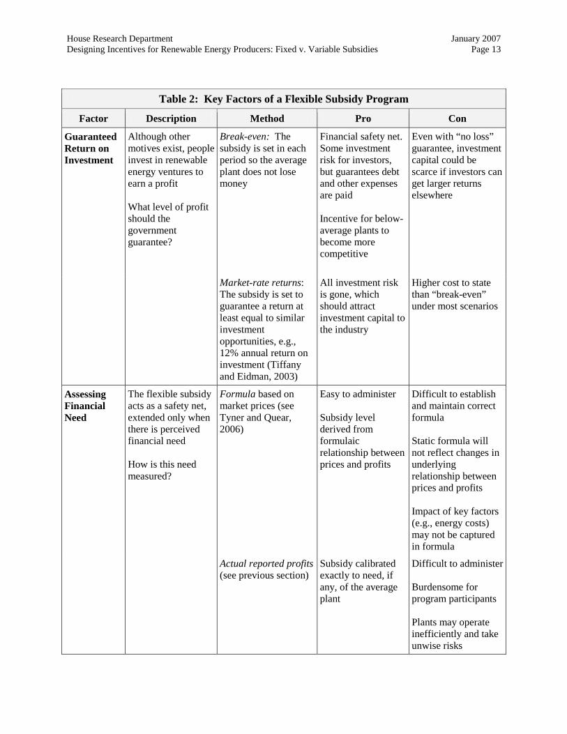
Table 2: Key Factors of a Flexible Subsidy Program

Factor Description Method Pro Con

Guaranteed Return on Investment

Although other motives exist, people invest in renewable energy ventures to earn a profit What level of profit should the government guarantee?

Break-even: The subsidy is set in each period so the average plant does not lose money

Financial safety net. Some investment risk for investors, but guarantees debt and other expenses are paid Incentive for below-average plants to become more competitive

Even with “no loss” guarantee, investment capital could be scarce if investors can get larger returns elsewhere

Market-rate returns: The subsidy is set to guarantee a return at least equal to similar investment opportunities, e.g., 12% annual return on investment (Tiffany and Eidman, 2003)

All investment risk is gone, which should attract investment capital to the industry

Higher cost to state than “break-even” under most scenarios

Assessing Financial Need

The flexible subsidy acts as a safety net, extended only when there is perceived financial need How is this need measured?

Formula based on market prices (see Tyner and Quear, 2006)

Easy to administer Subsidy level derived from formulaic relationship between prices and profits

Difficult to establish and maintain correct formula Static formula will not reflect changes in underlying relationship between prices and profits Impact of key factors (e.g., energy costs) may not be captured in formula

Actual reported profits (see previous section)

Subsidy calibrated exactly to need, if any, of the average plant

Difficult to administer Burdensome for program participants Plants may operate inefficiently and take unwise risks

House Research Department January 2007 Designing Incentives for Renewable Energy Producers: Fixed v. Variable Subsidies Page 14 One key parameter to set is the level of guaranteed return on investment in the renewable energy operation. Because variable subsidies provide a financial safety net, they effectively eliminate much of the investment risk for investors. But what is the proper level of return? Here are two options:

Break-even: With a break-even level of guaranteed return, subsidies are paid so that expenses just match revenues plus subsidies when the plant is losing money. No dividends are paid to investors. Basic economic theory implies that in the long run, rational people will only invest their money where they can receive a rate of return at least equal to the rate they could achieve from similar investment opportunities. Ethanol profits are volatile, and a market-rate return on investment may be required to obtain startup equity capital. However, it is believed that it was not an intolerable level of investment risk but a lack of lenders willing to loan money to inexperienced farmers that inhibited ethanol production in Minnesota prior to the advent of the producer payment program in 1987. If that is true, guaranteeing break-even profits in lean years—where principal and interest payments are included as expenses in the calculation of net margins—might be sufficient to propel the industry forward.

Market-rate returns: Subsidies could theoretically be calibrated to guarantee a minimum return on investment. By taking away the investment risk and guaranteeing a market-rate return, this approach should attract plenty of eager investors. However, under most scenarios, this approach will be more costly than the “break-even” approach. For instance, when the plant is operating at a modest profit, payments may still be made to lift the profit margin up to the guaranteed rate of return.

Setting the proper rate of return is further complicated under both methods by the fact that investors may gain positive returns even in “bad” years due to tax write-offs, etc. Under a flexible subsidy system, government aid is a safety net, extended only when there is perceived financial need. But measuring actual need could be difficult. Here are two possible approaches:

Formula-based approach: This approach requires a firm understanding of the impact of changing input and output prices on profits, as captured in a formula used to calculate the appropriate level of subsidy in each period. Producers are guaranteed a minimum return or profit, and the subsidy is set to achieve this profit given the current level of corn and ethanol prices. This approach is illustrated most clearly by Tyner and Quear. This method would be fairly easy to administer. Once the formula is established, the program administrator enters current information on corn and ethanol prices and the formula returns the appropriate level of subsidy, if any, required for owners to achieve the guaranteed per-gallon level of return.

However, creating and maintaining a proper formula could be difficult. The fundamental relationships imbedded in the formula are likely to hold over time (e.g., higher corn prices mean lower ethanol profits, holding all other factors constant). But differences in size between plants and changes in production capacity and other factors would alter the


true relationship between corn and ethanol prices and profits.17 More importantly, fluctuations in factors not captured in the formula could have a significant impact on profits. For instance, when corn and ethanol prices are favorable, the formula would prescribe low or no subsidy. However, a spike in natural gas costs—not reflected in the subsidy calculation—could put some renewable energy operations in financial peril.18

Actual reported profits-based approach: This approach requires current financial information from all participating plants in each payment period. As in the formula-based approach, producers are guaranteed a minimum level of return or profit, but the level of subsidy is tied to reported net margins, not the assumed relationship between the market price of corn and ethanol and ethanol profits. Once each plant submits its financial data, an average margin per gallon is calculated for all participating plants. While precise, this method could be burdensome for both the administrating agency and program participants. Determining the per-gallon payment rate would require aggregating current financial data on all plants and calculating an average net margin/gallon. Assuming payments are issued four times a year, recipients would be required to submit quarterly, audited financial statements—an expensive and time-consuming proposition. Also, as pointed out in the last section, this safety net may encourage inefficiency and unwise risk taking on the part of plant owners.

A Four-Step Process for Identifying the Appropriate Subsidy Policy Should lawmakers consider creating a new program to assist renewable energy producers, the following basic four-step process could be used to identify alternatives, evaluate options, and select the preferred policy. 1. Identify the goal(s) of the subsidy policy: Is the goal to overcome a perceived failure in

the private lending market? Or to provide a financial safety net, essentially guaranteeing solvency in early or all years of operation? Is a secondary goal to support the industry at the lowest cost to the state? Who should receive the subsidy and under what circumstances will they be eligible?

17 For example, Tyner and Quear also use Tiffany and Eidman’s 2003 snapshot of ethanol profitability factors to create their variable subsidy system. As a result, their formula reflects the relationship between corn and ethanol prices and per-gallon profits for the average 40-million-gallon Minnesota ethanol plant in 2002. For that 40-million-gallon plant, when corn prices rise from $2.20 per bushel to $2.40 per bushel, profits slip 2¢ per gallon, holding all other factors constant. However, if that plant should expand to compete with some of the newer, larger plants being constructed in South Dakota and Nebraska today, the relationship between corn prices and profits will change. According to the Tiffany/Eidman model, a 20¢-per bushel jump in corn prices, holding all else constant, results in only a 1.2¢-per-gallon dip in ethanol profits when the same plant is producing 120 million gallons a year.

18 Again using the Tiffany/Eidman model, profits are estimated to be 8¢ per gallon when corn prices are $2.20 per bushel, ethanol prices are $1.15 per gallon, and natural gas prices are $4.50 per decatherm. Leaving corn and ethanol prices the same and increasing natural gas prices to $8 per decatherm (well within the $1.50 to $9 per decatherm range reported by Tiffany and Eidman), margins per gallon are -4¢.


2. Identify multiple subsidy alternatives: Will achieving the goal(s) in step 1 require

fixed payments, or could a system of variable payments work? Are there similar programs in other states or at the federal level that could serve as a model? Does the industry face unique conditions or constraints that should be considered? What kind of information is needed to administer each alternative? (e.g., variable payments tied to actual profit/loss margins may require audited financial statements for each period before any subsidy payments are made.)

3. Model the impact of each alternative program: Using available modeling tools,

estimate the impact and cost of each program against a backdrop of participation and economic scenarios.

4. Rank the alternatives and select a program: While the primary factor would be

success in achieving the goal(s) of step 1, additional criteria may include: a. compatibility with existing programs; b. programmatic clarity and ease of administration; c. size and predictability of the budgetary impact; d. economic efficiency; and e. equity or fairness as defined by lawmakers and citizen stakeholders. Although this process is presented here in stepwise fashion, in practice it may be iterative. For instance, the findings in step 4 may lead to a return to step 2 and brainstorming additional program options. These new options are then modeled in step 3 before returning to step 4 for comparison against existing alternatives. Conclusion Minnesota is a forerunner in the promotion of renewable fuels, writing the ethanol producer payment program into law 20 years ago. As new sources of domestic, renewable energy emerge, Minnesota lawmakers may find themselves again debating whether subsidies are needed to overcome perceived failures in the private marketplace and propel a promising industry forward. Should lawmakers decide a subsidy is in order, the distinction between fixed and variable subsidies outlined in this paper may help inform the debate.


Appendix A: Constructing the Hypothetical Ethanol Plant To illustrate how volatile ethanol profits can be, the author modeled annual profit levels for an imaginary ethanol plant. A model is a simplified representation of an actual system that captures, as best as possible, the most important relationships in the system and depicts how these relationships influence a certain outcome or result. In this case, the system is an ethanol plant and the outcome is the level of profit per gallon, as influenced by fluctuations in expenses, revenues, and operating efficiency and size. The model used is an extension of the paper and spreadsheet (“BuGal”) created by Douglas Tiffany and Vernon Eidman of the University of Minnesota. The authors interviewed dozens of industry experts—including the owners and operators of Minnesota’s ethanol plants—and created a thorough and accurate snapshot of the dry-mill ethanol production process in Minnesota in 2002. In doing so, they created a spreadsheet that shows in detail all of the costs and revenues associated with turning corn into motor fuel. Through their further analysis, they ascertained the relative importance of each of these line items, settling on a handful of factors that have the greatest impact on ethanol profits. These five key factors are:

• corn prices; • ethanol prices; • natural gas prices; • the conversion factor (i.e., number of gallons of ethanol derived from a bushel of

corn); and • the capacity factor (i.e., percent of nameplate plant capacity produced each year).

Because their work depicts a modern, 40-million-gallon capacity dry-mill plant as of 2002, their spreadsheet was modified in several ways. The goal was to use the 2002 snapshot, as modified, to estimate the profitability of the same plant for the years 1987 to 2005. To do so, actual annual cost and revenue data, where available, were substituted for the first three key factors Tiffany and Eidman identified. Importantly, the “BuGal” was also modified to include payments of debt principal as an operating expense in the calculation of net margin per gallon. As a result, net margins of zero or greater should mean the owners could make scheduled debt payments, both principal and interest. Due to a circular reference error in Microsoft Excel, the author also eliminated Tiffany and Eidman’s arguably more realistic calculation of principal expenses including additional “sweep” payments (i.e., excess principal payments some lenders require plant owners to make in profitable years). A straight-line method was used to estimate annual principal payments instead. A list of other assumptions is included below. Any errors that result from modifying BuGal are the author’s.

House Research Department January 2007 Designing Incentives for Renewable Energy Producers: Fixed v. Variable Subsidies Page 18 Data Sources

The sources of the data substituted into the “BuGal” spreadsheet for each program year are depicted in Table A-1. All other data used to calculate net margins in “BuGal” (e.g., the price of propane, enzymes, labor, etc.) were left as they are and reflect prices in 2002. These items are considered of lesser importance to the profitability of an ethanol plant. For the data substituted, statewide averages were frequently used. The average annual price paid/received by an actual plant could vary significantly from the average statewide prices. When a full data series for the years 1987 to 2005 was not available, the missing data was estimated using a simple linear regression equation.

Table A-1: Data Sources and Linear Regression Equations Used

Price data (annual average)

Source Missing Years

Linear Regression Equation Unadjusted R2

Corn (bushel) USDA, NASS None N/A N/A

Wholesale/rack ethanol (gallon)*

Minnesota Department of Agriculture (MDA)

None N/A N/A

Natural gas (thousand cubic feet (tcf))

U.S. Energy Information Administration

1987-1996 yt = .9312xt – 1.2285 where yt = Minn. industrial price/tcf in year t x = Minn. commercial price/tcf in year t

0.9809

DDGS (ton) USDA, Feed Situation and Outlook Yearbook (2005), data for Lawrenceburg, Indiana

1987-1994 yt = 41.281xt + 6.512 where y = DDGS/ton (Lawrenceburg) in year t x = No. 2 yellow corn/bushel (Minneapolis) in year t

0.7929

*Note: following Tiffany and Eidman’s convention, the ethanol prices used are net of freight, storage, and commission costs of $0.10/gallon. The source for DDGS prices is the same used by Tiffany and Eidman in their “If the last decade’s price history were to replay...” exercise. The method used to estimate missing DDGS values is the same used by Paulson, Babcock, Hart, and Hayes.19 The estimate of the blended interest rate for initial plant construction (9 percent) follows a common lending convention

19 Nick D. Paulson, Bruce A. Babcock, Chad E. Hart, and Dermot J. Hayes, “Insuring Uncertainty in Value-added Agriculture: Ethanol Production” (working paper 04-WP 360, Center for Agricultural and Rural Development, Iowa State University, 2004).

House Research Department January 2007 Designing Incentives for Renewable Energy Producers: Fixed v. Variable Subsidies Page 19 uncovered by Tiffany and Eidman in 2002—setting the rate at prime plus 75 basis points. The source for the average prime rate in 1987 and 2001 is the Federal Reserve Board. Construction costs were assumed to be $3 per gallon of capacity during new construction in 1987 and $0.50 per gallon of capacity added during the 2001 expansion.20 Plant Operating Assumptions

Several assumptions were made regarding the efficiency and production capacity of the plant from 1987 to 2005. Changing any of these assumptions will have an impact on the model’s output—profit per gallon—in any given year. Assumption #1: The profitability model developed by Tiffany and Eidman for Minnesota ethanol plants in 2002, when modified in specific ways, can derive a reasonable estimate for profitability for plants operating as early as 1987. It is debatable how well the profitability model for modern ethanol plants in 2002 reflects the realities of ethanol production in earlier and later program years. Production processes have almost certainly changed since the late 1980s. To be clear, the researchers don’t clam their findings can be used in this way—they extrapolate their findings forward ten years to derive profitability estimates, but they do not use BuGal to estimate profits in earlier years. Therefore, the profitability estimates in this paper should be seen as rough, at best. Assumption #2: The plant begins production in 1987 with a maximum capacity of 15 million gallons per year and expands to 40 million gallons in 2001. Records of producer payment outlays in the program’s early years reveal that the original plants were very small compared to those of today. In fact, it appears it isn’t until the FY1992-1993 biennium that any single plant is hitting the 15-million-gallon-per-year producer payment ceiling. The expansion timing is consistent with Tiffany and Eidman’s finding that most of Minnesota’s smaller 15-million-gallon ethanol plants expanded in the early part of this decade. Assumption #3: The plant’s annual production is less than nameplate capacity in the early years but eventually exceeds nameplate production capacity in subsequent years. Tiffany and Eidman found that many ethanol plants operate beyond their bonded, warranted nameplate production capacity, but doing so is not a given. Operating beyond nameplate capacity requires top-notch engineering and excellent management. They found that Minnesota’s plants operate with a capacity factor in the range of 80 percent to 150 percent of nameplate capacity, settling on 120 percent as an approximate midpoint. The hypothetical plant begins production in 1987 with a nameplate capacity of 15 million gallons and a factor of nameplate capacity of 90 percent. A major assumption underlying the model is that the plant becomes more efficient and produces at a higher capacity over time due to a combination of management ingenuity and improvements in inputs like the enzymes used in fermentation. Assuming, for the sake of simplicity, that production capacity improvements over

20 U.S. GAO, 1984; Hosein Shapouri and Paul Gallagher, USDA’s 2002 Ethanol Cost-of-Production Survey, USDA, Agricultural Economic Report Number 841, 2005.

House Research Department January 2007 Designing Incentives for Renewable Energy Producers: Fixed v. Variable Subsidies Page 20 the life of the plant are constant, the factor of capacity was set to grow at a constant 2.5 percentage points a year, hitting a peak of 120 percent in 2002 and remaining at that level until 2005. Similarly, over time the plant is assumed to operate more efficiently, extracting more ethanol from a bushel of corn (i.e., the conversion factor). Increased production means fixed costs like overhead and debt service are spread out over a larger number of gallons. This tends to increase net margin/gallon, holding other factors constant. In reality, production improvements may be more “chunky,” with sizeable jumps taking place occasionally, followed by years of little or no improvement. To the extent that the model does not accurately reflect the way production processes and capacity change in a real plant, the model will tend to over- or under-estimate profitability. Assumption #4: The model plant does not cut back or suspend production in the face of adverse market conditions. The model does not allow the option of cutting back or stopping production when the net margin is negative. As a result, the plant amasses large losses in bad years, leading to large subsidy costs, especially in Variable Subsidy Program #2. Assumption #5: For simplicity, all other federal, state, and local subsidies available to plant owners are left out in calculating profit. To the extent that actual plants utilize additional subsidies that lower construction costs or property taxes, increase margins, etc., the model used in this paper will underestimate per-gallon profits. Assumption #6: The effective interest rate for initial construction is the private lending rate only. Participation in subsidized government loan programs could lower the blended rate paid on debt financing from all public and private sources, reducing interest expenses and increasing net margins.


Appendix B: Equations Equations for Figures 1 and 2

Net Margin/gal.: The annual estimates of net margin (i.e., profit/loss) per gallon before producer payments come directly from the profitability model described in Appendix A. Net margin/gal. + fixed subsidy: The annual estimates of profit/loss plus the fixed producer payment of 20¢ per gallon is straightforward and calculated as follows:

nmft = nmt + .20

where nmft = net margin/gallon after the fixed subsidy for year t nm = net margin/gallon pre-subsidy (“Net Margin/gal.”) for year t

t = a given year in the range of 1987 to 2005 Net margin/gal. + variable subsidy #1: The equation for the final net margin/gal. with variable producer payments under system #1 is essentially the same as the fixed equation, except the 20¢-per-gallon subsidy is paid only when “Net Margin/gal.” is negative.

nmv1 t = nm t + .20 where nm t < 0 and nmv1t = nm t where nm t ≥ 0

where nmv1 t = net margin/gallon after the variable subsidy Net margin/gal. + variable subsidy #2: The equation for net margin per gallon with variable producer payments under system #2 sets the producer payment exactly equal to the actual loss per gallon. The net result is that the net margin after subsidy is at the break-even level, or $0 per gallon.

nmv2 t = nm t + (0 – nm t) where nm t < 0 and nmdvt = nm t where nm t ≥ 0


($0.60)

($0.40)

($0.20)

$0.00

$0.20

$0.40

$0.60

$0.80

$1.00

1987

1989

1991

1993

1995

1997

1999

2001

2003

2005

$/ga

l.

0

10,000,000

20,000,000

30,000,000

40,000,000

50,000,000

60,000,000

Gal

lons

Net margin/gal. Net margin/gal.+ fixed subsidy Gallons produced

Appendix C: What Happens When the Plant Outgrows the Program? Figures 1 and 2 display the impact of per-gallon subsidies on the first 15 million gallons produced each year. Although many of the plants built in Minnesota in the mid-1990s had a maximum production capacity of 15 million gallons per year or less, most expanded to 40 million gallons or so in the early part of this decade.21 Larger plants are more competitive; newly constructed plants are almost always 40 million gallons or larger with many closer to 100 million gallons. What impact does a fixed per-gallon subsidy, capped at the first 15 million gallons, have on the per-gallon profits of these larger plants? Figure C-1 shows the net margin/gallon for all gallons produced each year, along with an additional line depicting the hypothetical plant’s annual production level. When the plant expands from 15-million to 40-million-gallon nameplate production capacity in 2001, the pre- and post-fixed subsidy22 net margin lines converge, illustrating that as production well surpasses the number of gallons eligible for subsidy, the payment predictably has a diminished effect on per-gallon profits. Figure C-1: Ethanol margin (profit/loss) per gallon before and after subsidy payment (All gallons) Note: See Appendices A and B for information on formulas used and data sources.

21 Tiffany and Eidman, 2003. 22 Because the pre-subsidy net margin is positive in the later years, no subsidy payments would be made under

either of the variable subsidy programs.

House Research Department January 2007 Designing Incentives for Renewable Energy Producers: Fixed v. Variable Subsidies Page 23 Figure C-1 displays margins for all gallons produced. Two main points:

• The hypothetical plant’s production capacity expands from 15 million to 40 million gallons in 2001, approximately reflecting the expansion timing of several of Minnesota’s older ethanol plants. See line “Gallons produced.”

• Although payments have a marked effect on margins when production capacity hovers around 15 million gallons, the impact on net margin is much less when (1) pre-subsidy profits are sizable, and (2) the 2001 plant expansion spreads the impact of the payments over more gallons. See the convergence between “Net margin/gal.” and “Net margin/gal. + fixed subsidy” after the 2001 capacity expansion.


Appendix D: Other States’ Producer Incentives Twenty-one states offer biofuel (mainly ethanol and biodiesel) producers incentives based on the number of gallons produced in a given period. Only North Dakota employs a flexible subsidy based on current market prices. The per-gallon subsidy level may vary in Montana as well, but the formula is based on the origin of the biomass feedstock (e.g., corn). State programs vary in size, scope, and expiration date. Of note, although the states below have authorized producer subsidies, in practice some may not be funded and/or administered as defined in law.

Table D-1: States with Flexible Per-Gallon Producer Subsidies State Incentive

Type Factor Description Citation

Montana Tax incentive/ payment

Origin of feedstock

Distributors/producers of fuel alcohol are eligible for “tax incentive payments” of $0.20/gallon if the alcohol is produced from 100% Montana products. The amount is reduced proportionately based on the percent of feedstock not sourced in Montana.

Montana Code Annotated

2005, §15-70-522

North Dakota

Payment Market prices

Owners of certain expanding ethanol plants are eligible for payments when the average price of corn exceeds $1.80/bushel and/or the average rack price of ethanol falls below $1.30/gallon.

North Dakota Century Code

2005, §4-14.1-08

Sources: U.S. Department of Energy, Alternative Fuels Data Center (accessed 12/21/06); and Doug Koplow, “Biofuels—At What Cost?”, The Global Studies Initiative, October 2006.

Table D-2: States with Fixed Per-Gallon Producer Subsidies (includes direct payments and tax credits)

Arkansas Kentucky Missouri Pennsylvania California Maine Montana South Dakota Hawaii Maryland Nebraska Texas Indiana Minnesota North Dakota Virginia Kansas Mississippi Oklahoma Wisconsin Wyoming Sources: U.S. Department of Energy, Alternative Fuels Data Center (accessed 12/21/06); and Doug Koplow, “Biofuels—At What Cost?”, The Global Studies Initiative, October 2006. Note: According to the sources cited, Montana and North Dakota have both fixed and flexible subsidy policies.

House Research Department January 2007 Designing Incentives for Renewable Energy Producers: Fixed v. Variable Subsidies Page 25 Many states, including some listed above as well as others that didn’t make the list, offer producer subsidies that are not tied to the number of gallons produced in a given period. Many states also provide biofuel-related incentives for fuel distributors/blenders and retailers that may indirectly benefit producers. For more information about ethanol, visit the agriculture area of our web site, www.house.mn/hrd/issinfo/agric.htm.

Documents

Designing Incentives for Renewable Energy Producers: Fixes v