© 2002 Eaton Corporation. All rights reserved.

Designing for System Reliability

Dave Loucks, P.E.Eaton Corporation

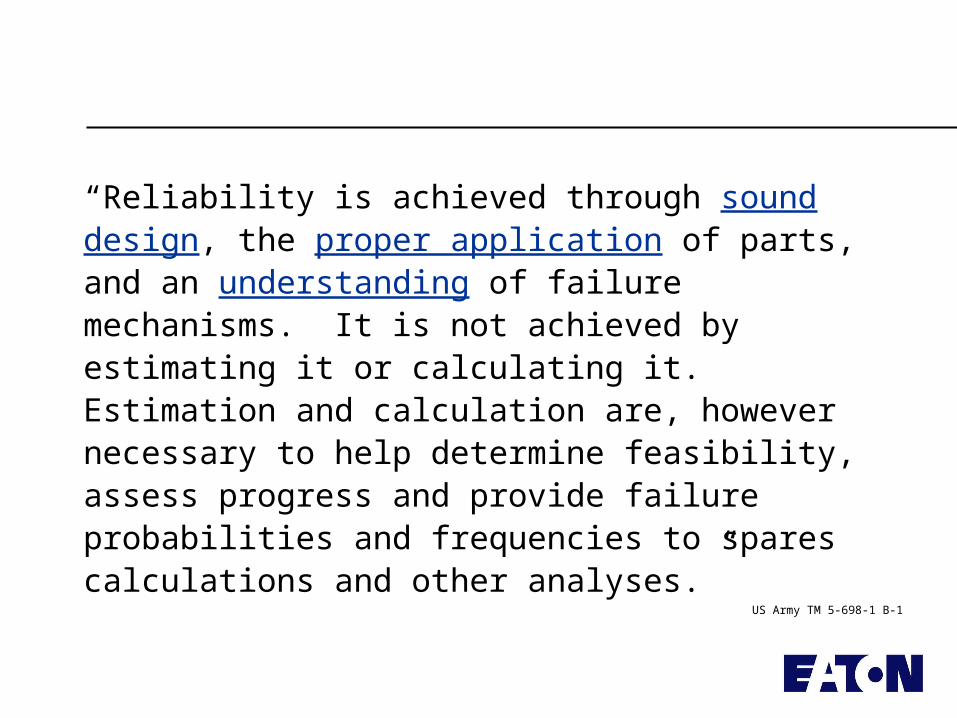
“Reliability is achieved through sound design, the proper application of parts, and an understanding of failure mechanisms. It is not achieved by estimating it or calculating it. Estimation and calculation are, however necessary to help determine feasibility, assess progress and provide failure probabilities and frequencies to spares calculations and other analyses.”

US Army TM 5-698-1 B-1

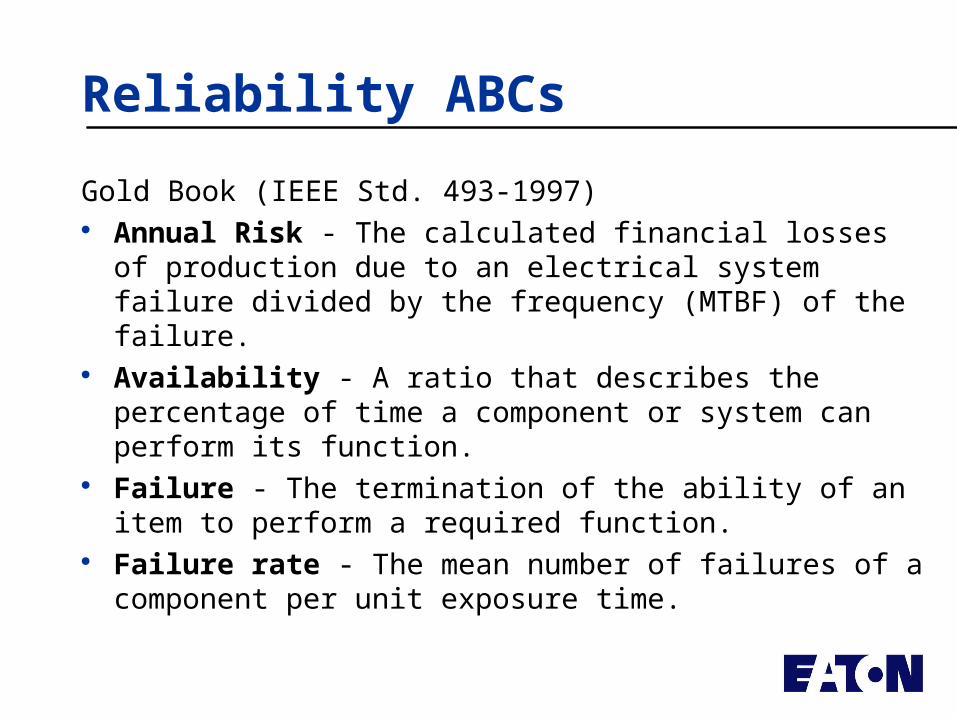
Reliability ABCs

Gold Book (IEEE Std. 493-1997) Annual Risk - The calculated financial losses of

production due to an electrical system failure divided by the frequency (MTBF) of the failure.

Availability - A ratio that describes the percentage of time a component or system can perform its function.

Failure - The termination of the ability of an item to perform a required function.

Failure rate - The mean number of failures of a component per unit exposure time.

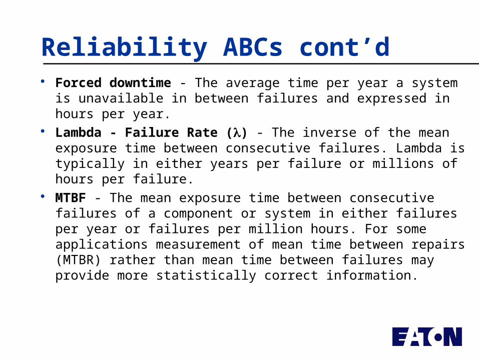
Reliability ABCs cont’d Forced downtime - The average time per year a system is

unavailable in between failures and expressed in hours per year. Lambda - Failure Rate () - The inverse of the mean exposure

time between consecutive failures. Lambda is typically in either years per failure or millions of hours per failure.

MTBF - The mean exposure time between consecutive failures of a component or system in either failures per year or failures per million hours. For some applications measurement of mean time between repairs (MTBR) rather than mean time between failures may provide more statistically correct information.

Designing for Reliability

Sound Design Proper Application of Parts (Components,

Systems) Understanding of Failure Mechanisms

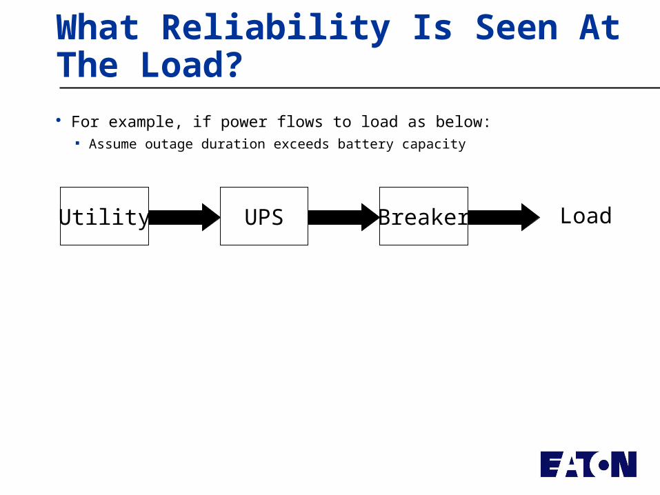
What Reliability Is Seen At The Load?

Utility UPS Breaker Load

For example, if power flows to load as below: Assume outage duration exceeds battery capacity

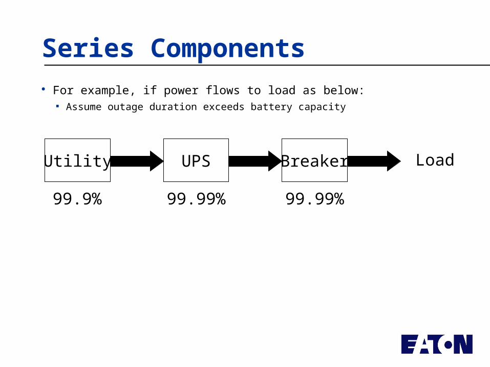
Series Components

Utility UPS Breaker Load

99.9% 99.99% 99.99%

For example, if power flows to load as below: Assume outage duration exceeds battery capacity

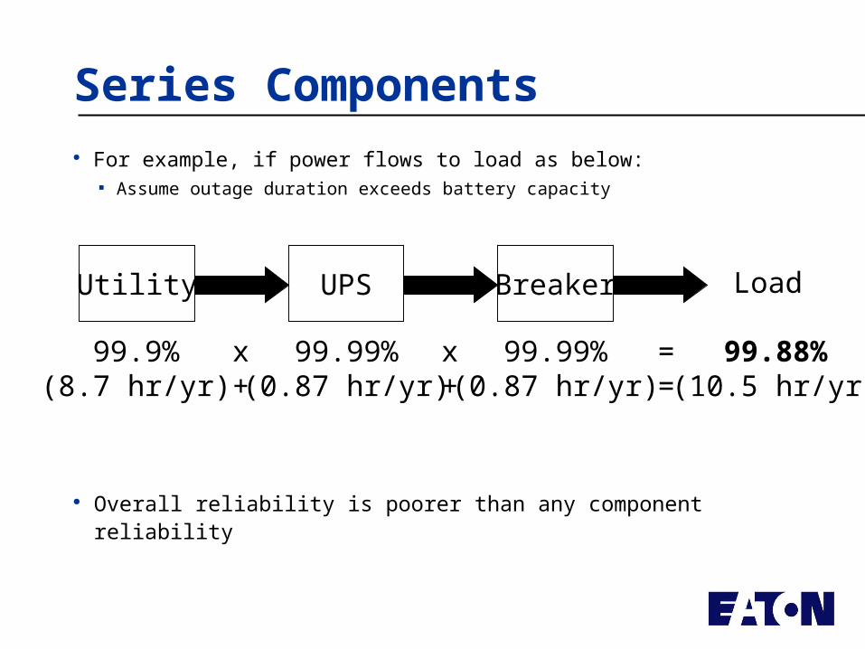
Series Components For example, if power flows to load as below:

Assume outage duration exceeds battery capacity

Utility UPS Breaker Load

99.9%(8.7 hr/yr)

99.99%(0.87 hr/yr)

99.99%(0.87 hr/yr)

x+

x+

==

99.88%(10.5 hr/yr)

Overall reliability is poorer than any component reliability

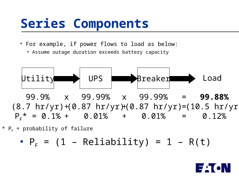
Series Components For example, if power flows to load as below:

Assume outage duration exceeds battery capacity

Utility UPS Breaker Load

99.9%(8.7 hr/yr)PF* = 0.1%

99.99%(0.87 hr/yr)

0.01%

99.99%(0.87 hr/yr)

0.01%

x++

x++

===

99.88%(10.5 hr/yr)

0.12%

PF = (1 – Reliability) = 1 – R(t)* PF = probability of failure

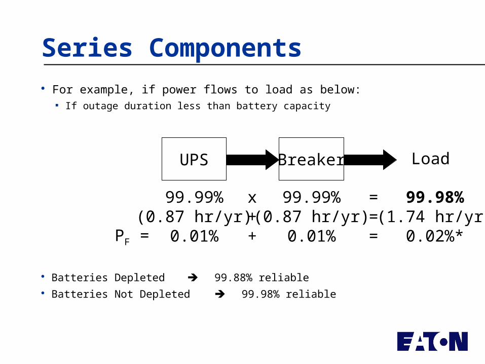
Series Components For example, if power flows to load as below:

If outage duration less than battery capacity

UPS Breaker Load

99.99%(0.87 hr/yr)

0.01%

99.99%(0.87 hr/yr)

0.01%

x++

===

99.98%(1.74 hr/yr)

0.02%*PF =

Batteries Depleted 99.88% reliable Batteries Not Depleted 99.98% reliable

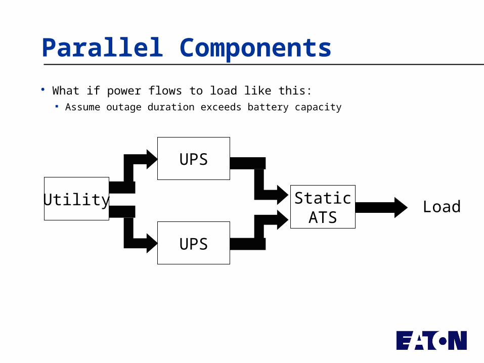
Parallel Components What if power flows to load like this:

Assume outage duration exceeds battery capacity

Utility

UPS

StaticATS

Load

UPS

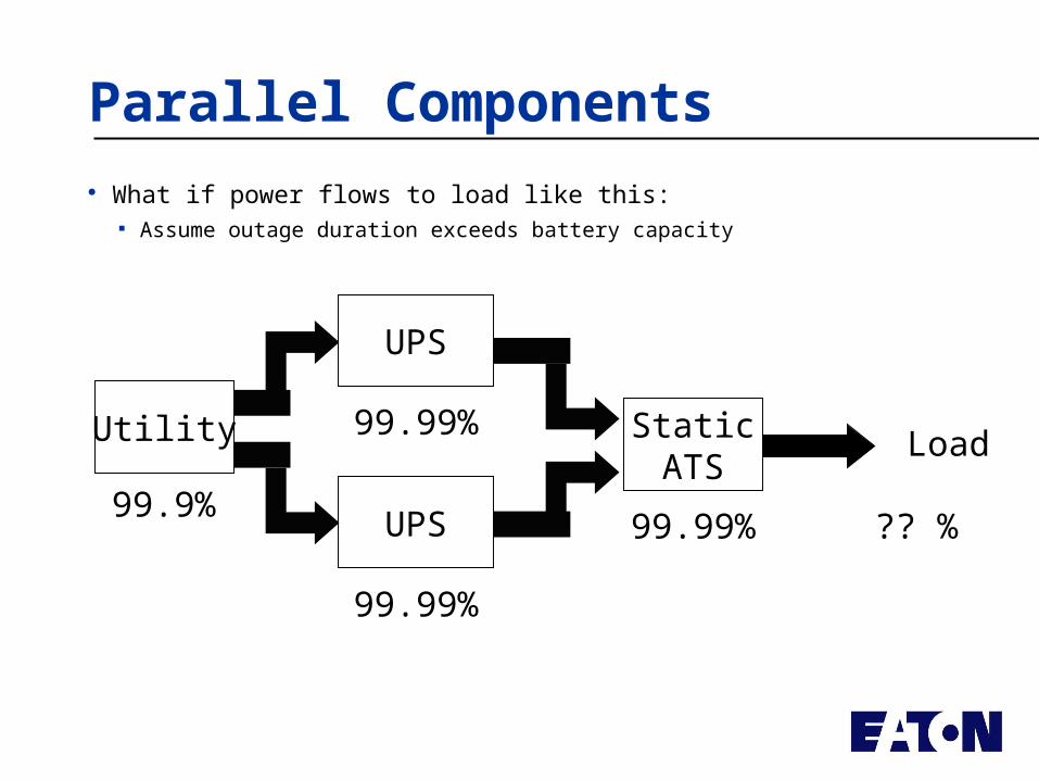
Parallel Components

Utility

UPS

StaticATS

Load

UPS99.9%

99.99%

99.99%

99.99%

?? %

What if power flows to load like this: Assume outage duration exceeds battery capacity

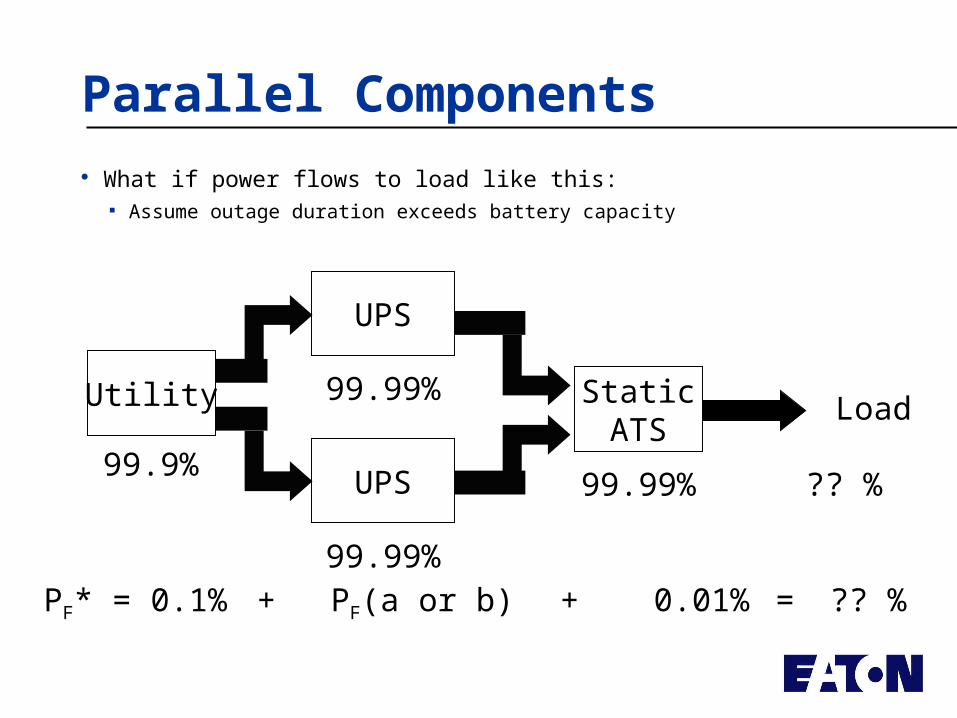
Parallel Components

Utility Load

99.9%

99.99%

99.99%

99.99%PF* = 0.1% PF(a or b)+ + = ?? %

?? %

UPS

StaticATS

UPS

0.01%

What if power flows to load like this: Assume outage duration exceeds battery capacity

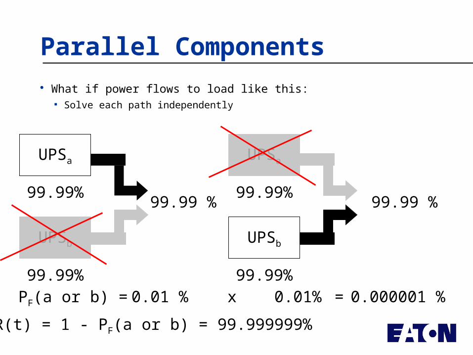
Parallel Components

99.99%

99.99%PF(a or b) = 0.01 % x = 0.000001 %

99.99 %

UPSa

UPSb

0.01%

What if power flows to load like this: Solve each path independently

99.99%

99.99%

UPSa

UPSb

99.99 %

R(t) = 1 - PF(a or b) = 99.999999%

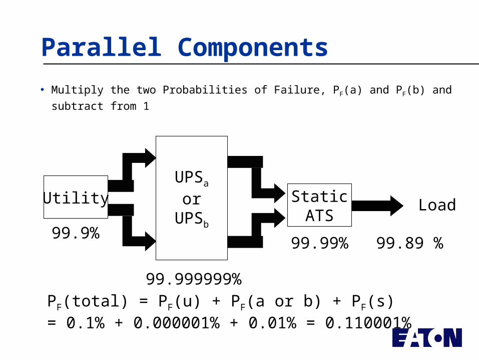
Parallel Components

Utility Load

99.9% 99.99%

99.999999%

99.89 %

UPSa

orUPSb

StaticATS

Multiply the two Probabilities of Failure, PF(a) and PF(b) and subtract from 1

PF(total) = PF(u) + PF(a or b) + PF(s)= 0.1% + 0.000001% + 0.01% = 0.110001%

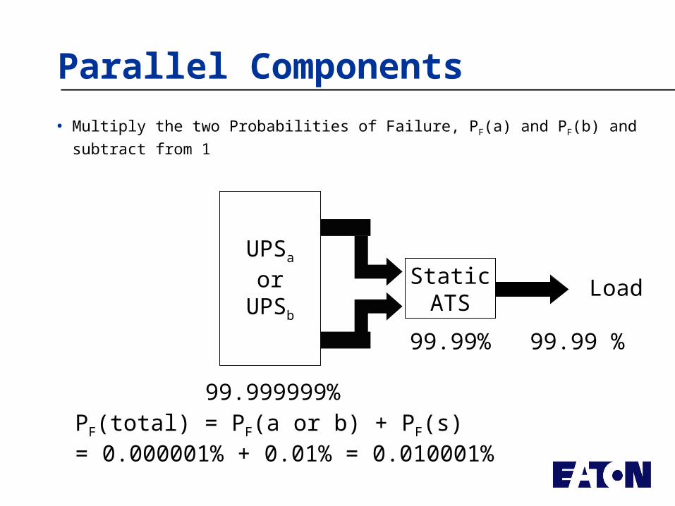
Parallel Components

Load

99.99%

99.999999%

99.99 %

UPSa

orUPSb

StaticATS

Multiply the two Probabilities of Failure, PF(a) and PF(b) and subtract from 1

PF(total) = PF(a or b) + PF(s)= 0.000001% + 0.01% = 0.010001%

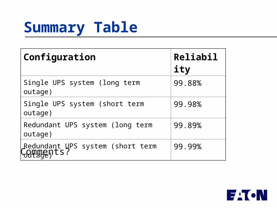
Summary Table

Configuration ReliabilitySingle UPS system (long term outage) 99.88%

Single UPS system (short term outage) 99.98%

Redundant UPS system (long term outage) 99.89%

Redundant UPS system (short term outage) 99.99%

Comments?

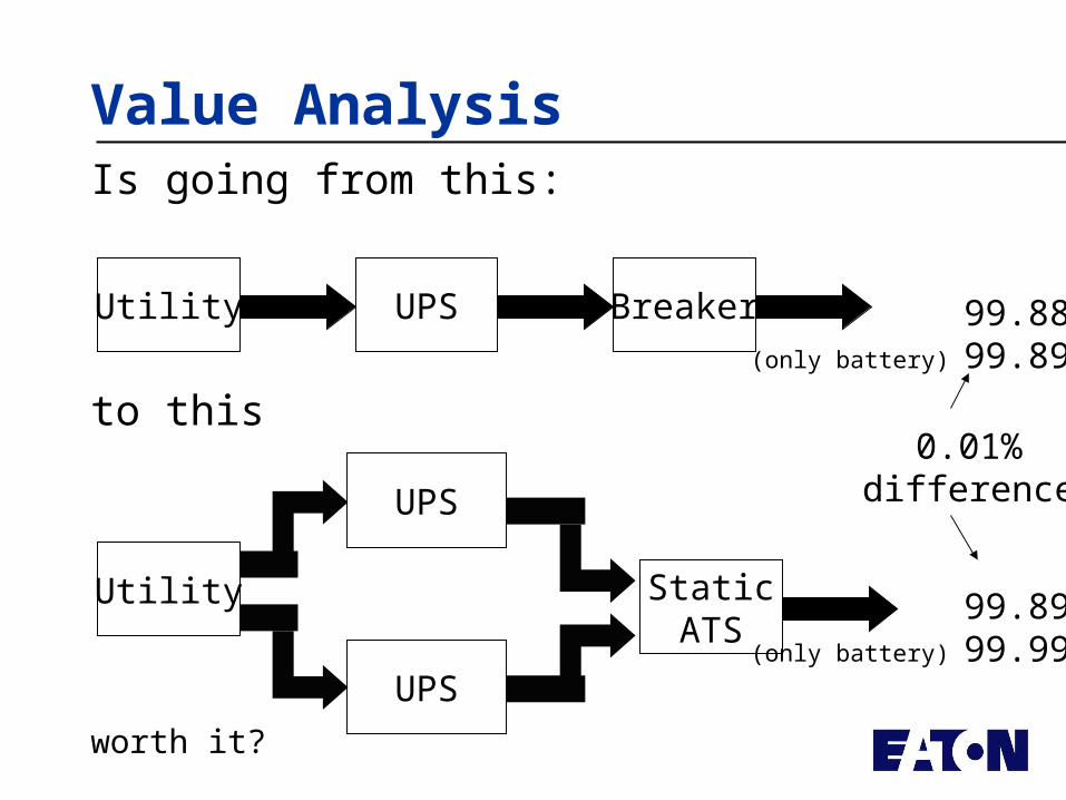
Value AnalysisIs going from this:

Utility UPS Breaker

Utility

UPS

StaticATS

99.89%(only battery) 99.99%

UPS

99.88%(only battery) 99.89%

to this

worth it?

0.01%difference

Value Analysis

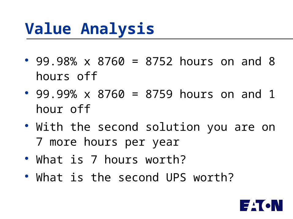
99.98% x 8760 = 8752 hours on and 8 hours off 99.99% x 8760 = 8759 hours on and 1 hour off With the second solution you are on 7 more

hours per year What is 7 hours worth? What is the second UPS worth?

Breakeven Analysis

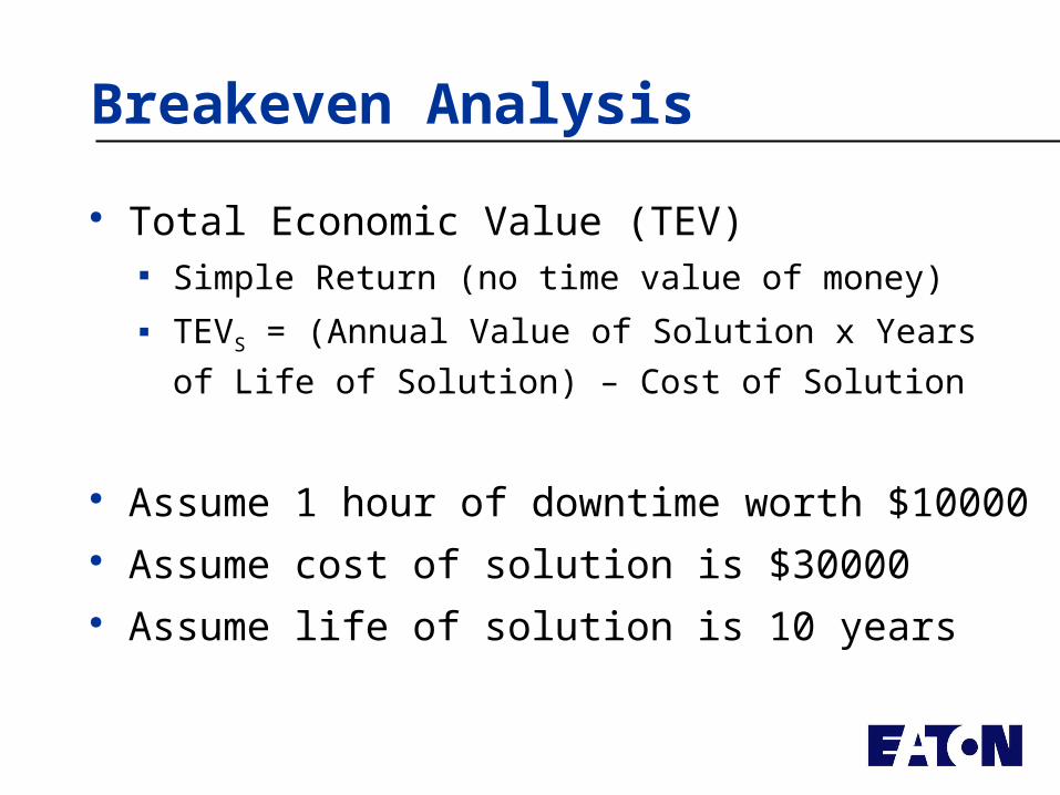
Total Economic Value (TEV) Simple Return (no time value of money) TEVS = (Annual Value of Solution x Years of Life of

Solution) – Cost of Solution

Assume 1 hour of downtime worth $10000 Assume cost of solution is $30000 Assume life of solution is 10 years

Breakeven Analysis

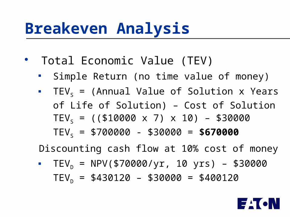
Total Economic Value (TEV) Simple Return (no time value of money) TEVS = (Annual Value of Solution x Years of Life of

Solution) – Cost of SolutionTEVS = (($10000 x 7) x 10) – $30000TEVS = $700000 - $30000 = $670000

Discounting cash flow at 10% cost of money TEVD = NPV($70000/yr, 10 yrs) – $30000

TEVD = $430120 – $30000 = $400120

Reliability Tools

Eaton Spreadsheet Tools IEEE PCIC Reliability Calculator Commercially Available Tools Financial Tools (web calculators)

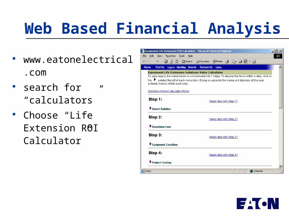
Web Based Financial Analysis www.eatonelectrical.com search for “calculators” Choose “Life Extension

ROI Calculator”

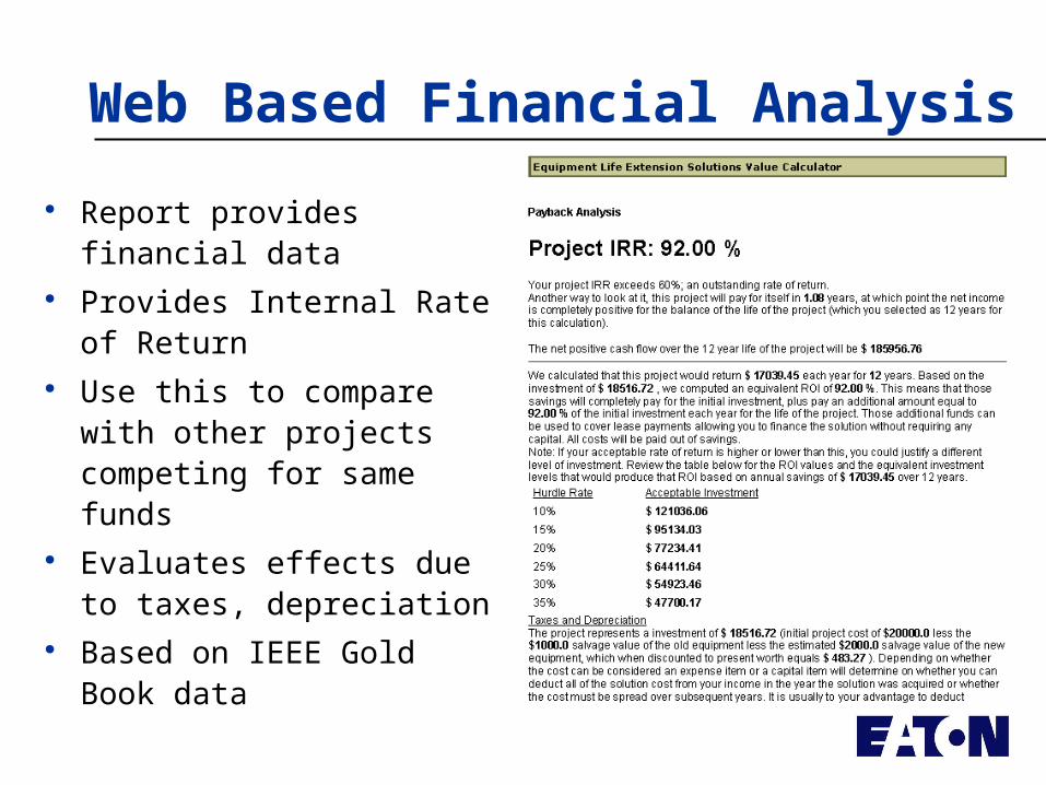
Web Based Financial Analysis Report provides financial

data Provides Internal Rate of

Return Use this to compare with

other projects competing for same funds

Evaluates effects due to taxes, depreciation

Based on IEEE Gold Book data

Uncertainty – Heart of Probability

Probability had origins in gambling What are the odds that …

We defined mathematics resulted based on: Events

• What are the possible outcomes? Probability

• In the long run, what is the relative frequency that an event will occur?

• “Random” events have an underlying probability function

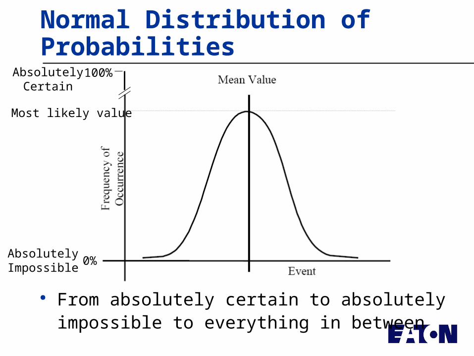
Normal Distribution of Probabilities

From absolutely certain to absolutely impossible to everything in between

AbsolutelyCertain

100%

0%AbsolutelyImpossible

Most likely value

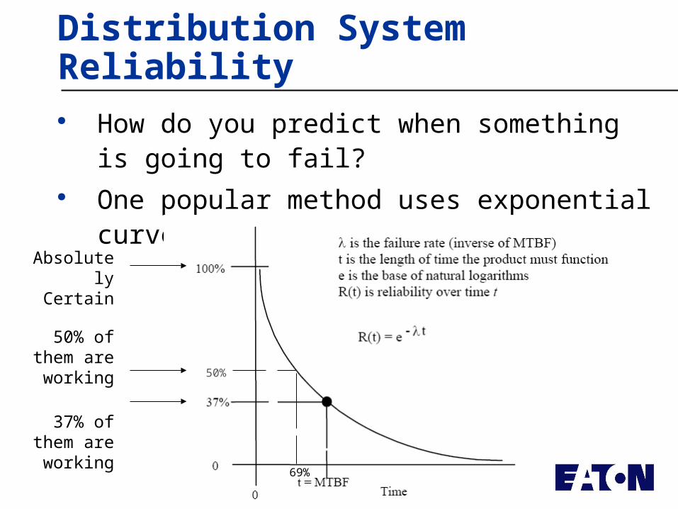
Distribution System Reliability How do you predict when something is going to

fail? One popular method uses exponential curve

AbsolutelyCertain

37% of them are working

50% of them are working

69%

50%

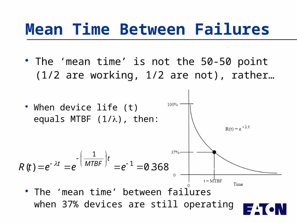
Mean Time Between Failures

The ‘mean time’ is not the 50-50 point (1/2 are working, 1/2 are not), rather…

When device life (t) equals MTBF (1/), then:

368011

.)(

eeetRt

MTBFt

The ‘mean time’ between failures when 37% devices are still operating

MTBF Review Remember, MTBF doesn’t say that when the

operating time equals the MTBF that 50% of the devices will still be operating, nor does it say that 0% of the devices will still be operating. It says 37% (e-1) of them will still be working.

Said another way; when present time of operation equals the mean (1/2 maximum life), the reliability is 37%

Exponential Probability

Assumes (1/MTBF) is constant with age For components that are not refurbished, we

know that isn’t true. Reliability decreases with age ( gets bigger)

However, for systems made up of many parts of varying ages and varying stages of refurbishment, exponential probability math works well.

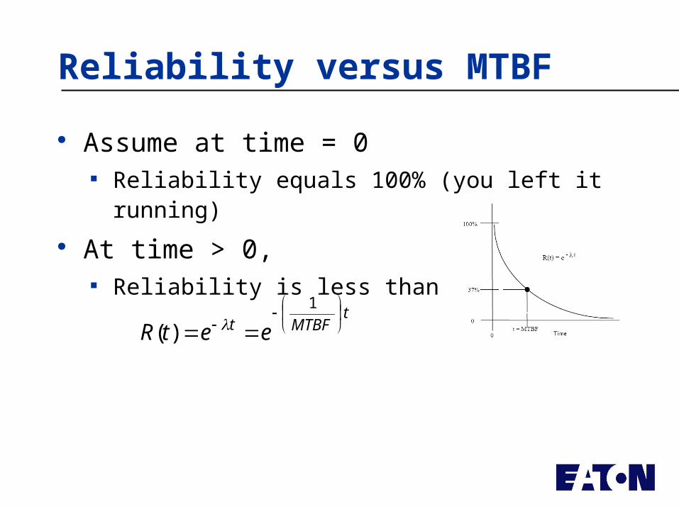
Reliability versus MTBF

Assume at time = 0 Reliability equals 100% (you left it running)

At time > 0, Reliability is less than 100%

tMTBFt eetR

1

)(

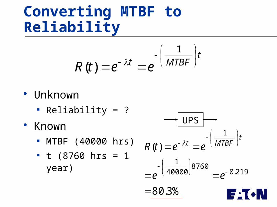
Converting MTBF to Reliability

Unknown Reliability = ?

Known MTBF (40000 hrs) t (8760 hrs = 1 year)

tMTBFt eetR

1

)(

UPS

%.

)(

.

380

21908760

400001

1

ee

eetRt

MTBFt

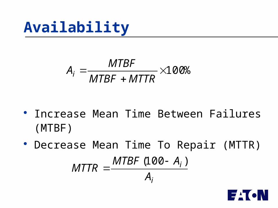
Availability

Increase Mean Time Between Failures (MTBF) Decrease Mean Time To Repair (MTTR)

%100

MTTRMTBF

MTBFAi

i

i

AAMTBF

MTTR)(

100

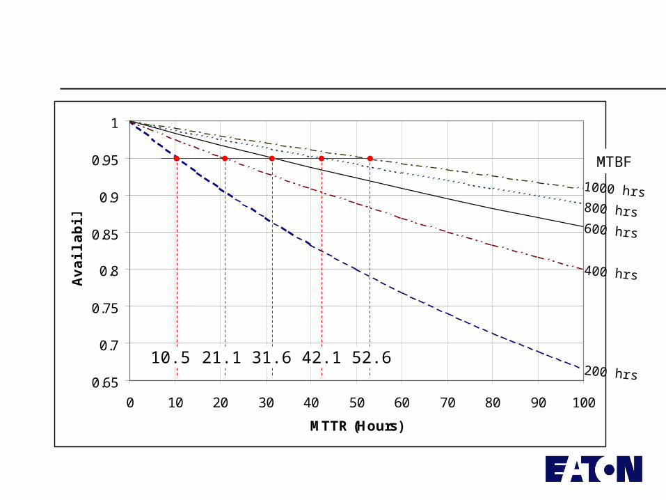
0.65

0.7

0.75

0.8

0.85

0.9

0.95

1

0 10 20 30 40 50 60 70 80 90 100

MTTR (Hours)

Avai

labi

lity

1000 hrs800 hrs600 hrs

400 hrs

200 hrs

MTBF

0.65

0.7

0.75

0.8

0.85

0.9

0.95

1

0 10 20 30 40 50 60 70 80 90 100

MTTR (Hours)

Avai

labi

lity

1000 hrs800 hrs600 hrs

400 hrs

200 hrs

MTBF

10.5 21.1 31.6 42.1 52.6