Designing and Implementation of Algorithms on MATLAB for ...Designing and Implementation of Algorithms on MATLAB for Adaptive Noise Cancellation from ECG Signal Hemant Kumar Gupta

International Journal of Computer Applications (0975 – 8887)

Volume 71– No.5, May 2013

1

Designing and Implementation of Algorithms on MATLAB for Adaptive Noise Cancellation from ECG

Signal

Hemant Kumar Gupta Ritu Vijay,Ph.D Neetu gupta JECRC UDML College of Engineering, Banasthali University, Rajasthan College of Engineering Jaipur, Rajasthan, India – 302022 Banasthali,Jaipur, Rajasthan, for Women , Jaipur, Rajasthan

ABSTRACT

The medical monitoring devices are more sensitive for the

biomedical signal recording and need more accurate results

for every diagnosis. The low frequency signal is destroyed by

power line interference of 50 Hz noise, this noise is also

source of interference for biomedical signal recording. The

frequency of power line interference 50 Hz is nearly equal to

the frequency of ECG, so this 50 Hz noise can destroyed the

output of ECG signal. One way to remove the noise is to filter

the signal with a notch filter at 50 Hz. However, due to slight

variations in the power supply to the hospital, the exact

frequency of the power supply might (hypothetically) wander

between 47 Hz and 53 Hz. A static filter would need to

remove all the frequencies between 47 and 53 Hz, which

could excessively degrade the quality of the ECG since the

heart beat would also likely have frequency components in the

rejected range. To circumvent this potential loss of

information, an adaptive filter has been used. The adaptive

filter would take input both from the patient and from the

power supply directly and would thus be able to track the

actual frequency of the noise as it fluctuates [2].

Keywords: Biomedical signals, Physiological, signal Processing, EMG

Signals, Diagnostic Instrumentation.

INTRODUCTION The electrocardiograph (ECG) is an instrument, which records

the electrical activity of the heart. ECG provides valuable

information about the wide range of the cardiac disorders such

as the presence of an inactive part or an enlargement of heart

muscle. ECG is used in characterization laboratory, coronary

care unit and for routing diagnostic application in cardiology.

Although the electric field generated by the heart can be best

characterized by vector quantity, its generally convenient to

directly measured only scalar quantity, a voltage difference of

mV order between the given point of the body. Most of the

electrophysiological signals have frequencies between dc (0

Hz) and 3000 Hz and amplitudes ranging between 10

microvolt‟s and 10 milli-volts [3][1] as shown in Table 1,

below.

Table 1 Electrophysiological Signals

Signal Biological

source

Average

amplitude

Frequency

Electrocardiogram

(ECG)

Heart 1-5 mV 0.05-100

Hz

Electroencephalogra

m (EEG)

Brain 10-50 V 0-150 Hz

Electromyogram

(EMG)

Muscles 0.1-1 mV 40-3000 Hz

Electrooculogram

(EOG)

Eyeball 0.05-3.5

mV

0-125 Hz

The amplifier and writing part should fatefully reproduce

signal in this range. A good low frequency response is

essential to ensure the stability of baseline. Due to their low

levels and their frequency spectra, these signals can be easily

swamped out by noise pick-ups from the power lines So

before these signals can be further processed to establish the

diagnostic values, their signal-to-noise ratio must be improved

by removing the contaminating 50 Hz interference from the

power line.

Since there is a spectral overlap between the desired signals

and interfering 50 Hz from electric power system, the removal

of power line interference must be such that the diagnostic

information in the frequency range around 50 Hz is less

affected.

Significant Features of ECG Waveform: A typical scalar

electrocardiographic lead is shown in Fig.1, where the

significant features of the waveform are the P, Q, R, S, and T

waves, the duration of each wave, and certain time intervals

such as the P-R, S-T, and Q-T intervals. ECG signal is

periodic with fundamental frequency determined by the

heartbeat. Each significant feature of ECG signal can be

represented by shifted and scaled versions one of these

waveforms as shown below [4].

QRS, Q and S portions of ECG signal can be represented

by triangular waveforms.

P, T and U portions can be represented by triangular

waveforms.

Once each of these portions generated, they can be added

finally to get the ECG signal. So the generated output ECG

signal by MATLAB is shown in Fig.2.

Fig.1 Typical one-cycle ECG signal



2

.

Fig.2 Typical ECG output waveform simulated in

MATLAB

Objective

This study mainly deals with the various aspects of Adaptive

Noise Cancellation and usage in different applications. The

major objectives of this thesis can be listed as follow:

• This task involves the study of the principle of Adaptive

Noise Cancellation and its Applications.

• Cancellation of Electric power noise (50 Hz) from ECG

signal by the designing and implementation of different

adaptive algorithms based upon FIR filters using

MATLAB software [6].

• The LMS algorithm can be easily modified to normalized

step-size version known as the normalized LMS

algorithm. NLMS, not only provides a potentially faster

adaptive algorithm, but also guarantee a more stable

convergence response to variation of input signal power

Basic Structure of an Adaptive Filter

An adaptive is essentially a digital filter with self adjustment

characteristics. It consist of two distinct part a digital filter

with adjustable coefficient, and an adaptive algorithm, which

is used to adjust or modify the coefficient of the filter as

shown in Fig 3 where two input signal d(n) and u(n) are

applied simultaneously to the adaptive filtering system. The

signal d(n) is measured signal obtained using some sensor

(also called desired signal) and it is contaminated signal

containing both the actual signal and noise and interference

signal, assumed uncorrelated with each other. The signal u(n)

is reference input signal and is also obtained using some

sensor and it provide a measure of the contaminating signal

which is correlated in some way with noise and interference in

the measured signal.

In most adaptive system, digital filter used is FIR because of

simplicity and guaranteed stability. Mostly FIR filter is

implemented using direct form structure. However, lattice

structure is preferred in some application like speech signal

processing. The filter coefficient at time n is given by vector

w (n) of length M, where M represents length of FIR filter. As

filter is M tap, we consider M sample of input u(n) at time n

as another vector u(n) of M.

We can write

W (n) = [w0 (n)w1(n)…..wM-1(n)]T (1)

u(n)=[u(n)u(n-1)…..u(n-M+1)] (2)

The output filter

1

0

( ) ( ) ( ) ( ) ( )M

T

i

i

y n w n u n i w n u n

(3)

Fig. 3 Block diagram of an adaptive filter

Adaptive Algorithm

Least Mean Square (LMS) Algorithm

The LMS is an approximation of the steepest descent

algorithm, which uses an instantaneous estimate of the

gradient vector. The estimate of the gradient is based on

sample values of the tap input vector and an error signal. The

algorithm iterates over each tap weight in the filter, moving it

in the direction of the approximated gradient. The idea behind

LMS filters is to use the method of steepest descent to find a

coefficient vector n w which minimizes a cost function

[8][23].

The LMS algorithm can be explain as

The output y (n) of FIR filter structure can be obtained from

1

0

( ) ( ) ( )N

m

y n w m u n m

(4)

Where n is no. of iteration

The error signal calculated by Eq. (5.5)

e (n) = d(n) - y(n) ( 5)

The filter weights are updated from the error signal e (n) and

input signal u(n) as in Eq. (5.6)

w(n+1) = w (n) +µe (n) u (n) (6)

where w(n) is the current weight value vector, w(n+1) is the

next weight value vector, u(n) is the input signal vector, e(n)

is the filter error vector and μ is the convergence factor which

determine the filter convergence speed and overall behavior

[11].

LMS Algorithm

In practical application of adaptive filtering, a fixed step size

Algorithm is required for

(i) Easier implementation

(ii) Single adjustable parameters µ for controlling the

convergence rate but slow convergence.

Normalized LMS (NLMS) Algorithm

Normalized Least Mean Square (NLMS) is actually derived

from Least Mean Square (LMS) algorithm. The need to derive

this NLMS algorithm is that the input signal power changes in

time and due to this change the step-size between two

adjacent coefficients of the filter will also change and also

affect the convergence rate. Due to small signals this

convergence rate will slow down and due to loud signals this

convergence rate will increase and give an error. So to

overcome this problem, try to adjust the step-size parameter

with respect to the input signal power. Therefore the step-size

parameter is said to be normalized. When design the LMS

adaptive filter, one difficulty we meet is the selection of the

step-size parameter μ. The main drawback of the pure LMS

0 0.5 1 1.5 2 2.5-4

-3

-2

-1

0

1

2

3

4

Time [sec]

Vol

tage

[mV

]ECG signal



3

algorithm is that it is sensitive to the scaling of its input u (n).

This makes it very hard to choose a learning rate μ that

guarantees stability of the algorithm [25].

When the convergence factor μ is large, the algorithm

experiences a gradient noise amplification problem. In order

to solve this difficulty, the NLMS (Normalized Least Mean

Square) algorithm is used. The correction applied to the

weight vector w(n) at iteration n+1 is “normalized” with

respect to the squared Euclidian norm of the input vector u(n)

at iteration n. We may view the NLMS algorithm as a time-

varying step-size algorithm, calculating the convergence

factor μ as in Eq.5.7

2

( )( )

µ nc u n

(7)

where α is the NLMS adaption constant, which optimize the

convergence rate of the algorithm and should satisfy the

condition 0<α<2, and c is the constant term for normalization

and is always less than 1. The Filter weights are updated by

the Eq. (8).

2( 1) ( ) ( ) ( )

( )w n w n e n u n

c u n

(8)

Normalization algorithm results in smaller step size values

than the conventional LMS algorithm. The normalized

algorithm usually converges faster than the LMS algorithm,

since it utilizes a variable convergence factor aiming at the

minimization of the instantaneous output error.

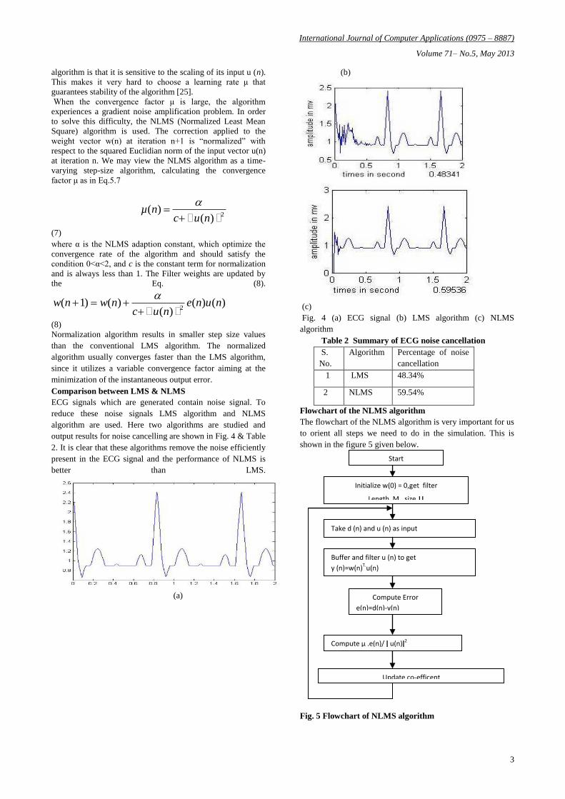
Comparison between LMS & NLMS

ECG signals which are generated contain noise signal. To

reduce these noise signals LMS algorithm and NLMS

algorithm are used. Here two algorithms are studied and

output results for noise cancelling are shown in Fig. 4 & Table

2. It is clear that these algorithms remove the noise efficiently

present in the ECG signal and the performance of NLMS is

better than LMS.

(a)

(b)

(c)

Fig. 4 (a) ECG signal (b) LMS algorithm (c) NLMS

algorithm

Table 2 Summary of ECG noise cancellation

S.

No.

Algorithm Percentage of noise

cancellation

1 LMS 48.34%

2 NLMS 59.54%

Flowchart of the NLMS algorithm

The flowchart of the NLMS algorithm is very important for us

to orient all steps we need to do in the simulation. This is

shown in the figure 5 given below.

Fig. 5 Flowchart of NLMS algorithm

Start

Initialize w(0) = 0,get filter

Length M, size μ

Compute Error

e(n)=d(n)-y(n)

Update co-efficent

w(n+1)=w(n)+ μe(n) /ǀ u(n) ǀ2

Compute μ .e(n)/ ǀ u(n)ǀ2

2

Take d (n) and u (n) as input

Buffer and filter u (n) to get

y (n)=w(n)T.u(n)



4

Adaptive Filter Algorithms

In these code segments, the purpose need to obtain is

processing and performing the LMS and NLMS algorithms.

The comparison below between the theories the simulation

parts (MATLAB code) may bring the better understanding

about not only the algorithm but the programming work.

The summary of the algorithms (LMS, NLMS) and the code

segments are demonstrated in the given below.

SIMULATION:

Implementations of LMS Algorithm:

Initialization: If prior knowledge of the tap weight

vector w(n) is available, use it to select an

appropriate value for w(n),otherwise, set w(0)=0.

Take,0<u<(1/M, Smax) Where: Smax=the maximum

value of PSD of the tap input u(n)

Data:

Give u (n) = M by 1 tap input vector at

time n,

d (n) = desired response at time n

To be computed: w (n) = estimate of tap-weight vector at

time n

Computation: y (n) = w (n).u(n)

e(n) = d(n) - y(n)

w (n+1) = w (n) +µ.e (n).u (n)

Table 3 Least Mean Square (LMS) algorithm

S.

No.

LMS algorithm

1 Initial Conditions

:

0< µ < 1

Length of Adaptive

filter=L

Input vector:

u[0,0,0…0]T

Wight vector:

w[0,0,0…0]T

For each instant

of time, n = 1,

2,…, compute:

= 1, 2, 3…, compute:

2 Output signal: y(n) = wT . u(n);

3 Estimation Error: e(n) = d(n)-y(n);

4 Tap-Weight

Adaptation:

w (n+1) = w + 2 µ

.e(n).u(n);

Implementations of NLMS Algorithm

In standard form of least mean square (LMS) filter in

adjustment applied to the tap weight vector of the filter at

iteration n consist of product of three terms:

(i) The step size parameter µ, which is under the

designer‟s control.

(ii) The tap input vector u(n),which is supplied by a

source of information.

(iii) The estimation error e(n),which is calculated at

iteration n.

The adjustment is directly proportional to the tap input vector

u(n). Therefore, when u(n) is large, the LMS filter suffer

from gradient noise amplification problem. Also, the

maximum step size u guarantee stability signal, u (n). One

important technique for optimizing speed of convergence

while maintaining the adjustment applied to tap weight vector

at iteration n+1 is „normalized‟ with respect to the squared

Euclidean norm of the tap –input vector u(n) at iteration n –

hence the term “normalized”. It can be briefly described as

follows:

Initialization: If prior knowledge of the tap weight

vector w(n) is available, use it to select an

appropriate value for w(0), otherwise set w(0)=0.

Take, 0<

<2(E[ǀ u (n) ǀ2 ]D (n)/E [ ǀ e (n) ǀ 2]);

where , E[ǀ u (n) ǀ2 ] = input signal power , E [ ǀ e (n)

ǀ 2] = error signal power , D (n) mean square

deviation of weight vector.

Data :

Given u (n) =M by 1 tap input vector at time n.

d (n) = desired response at time n.

To be computed

w(n) = estimate of tap-weight vector at time n.

Computation: y (n) = w (n)T. u (n)

e(n) = d(n) - y(n)

w (n+1) = w (n) +µ.e (n).u (n)/

u(n) 2

The algorithm required 2*M+1 addition and 2*M+1

multiplication at any iteration n where M is the tap length or

filter order. The computation complexity depends on the

order of the filter and it must be carefully chosen. The

following figure shown the flow chart to implement the

algorithm

Table 4 Normalized Least Mean Square (NLMS)

algorithm

S.No

NLMS

Al algorithm

1 Initial Conditions: 0< α < 2 and c is small constant.

Length of Adaptive filter=L

Input vector: u[0,0,0…0]T

Wight vector: w[0,0,0…0]T

For each instant of time, n = 1, 2,…, compute:

2 Output signal: y(n) = wT . u(n);

3 Estimation Error: e(n) = d(n)-y(n);

4 adaption step size: w(n)+[2 α/c+u(n)T.u(n)]e(n)u(n)

w (n+1) = w + 2 µ .e(n).u(n);



5

Results:

LMS algorithm: In this case µ =0.05, Filter length is 15, 20,

25 and 1400 iterations Fig. 6, 7, 8 given below.

Figure 6 LMS algorithm where µ=0.05, Filter length = 15

Fig.7 LMS algorithm where µ=0.05, Filter length=20

Fig. 8 LMS algorithm where µ=0.05, Filter length = 25

LMS algorithm: In this case µ =0.09, Filter length is 15, 20,

25, 35 and 1400 iterations Fig. 9, 10, 11 given below.

Fig. 9 LMS algorithm where µ=0.09, Filter length =

15

0 200 400 600 800 1000 1200 1400-1

0

1Input ECG Signal

0 200 400 600 800 1000 1200 1400-2

0

2 ECG signal+50 Hz noise

0 200 400 600 800 1000 1200 1400-2

0

2 Recover using LMS Filterd Output

0 200 400 600 800 1000 1200 1400-1

0

1Input ECG Signal

0 200 400 600 800 1000 1200 1400-2

0


0 200 400 600 800 1000 1200 1400-2

0


0 200 400 600 800 1000 1200 1400-1

0

1Input ECG Signal

0 200 400 600 800 1000 1200 1400-2

0


0 200 400 600 800 1000 1200 1400-2

0


0 200 400 600 800 1000 1200 1400-1

0

1Input ECG Signal

0 200 400 600 800 1000 1200 1400-2

0


0 200 400 600 800 1000 1200 1400-2

0




6

Fig. 10 LMS algorithm where µ=0.09, Filter length =

20

Fig. 11 LMS algorithm where µ=0.09, Filter length = 25

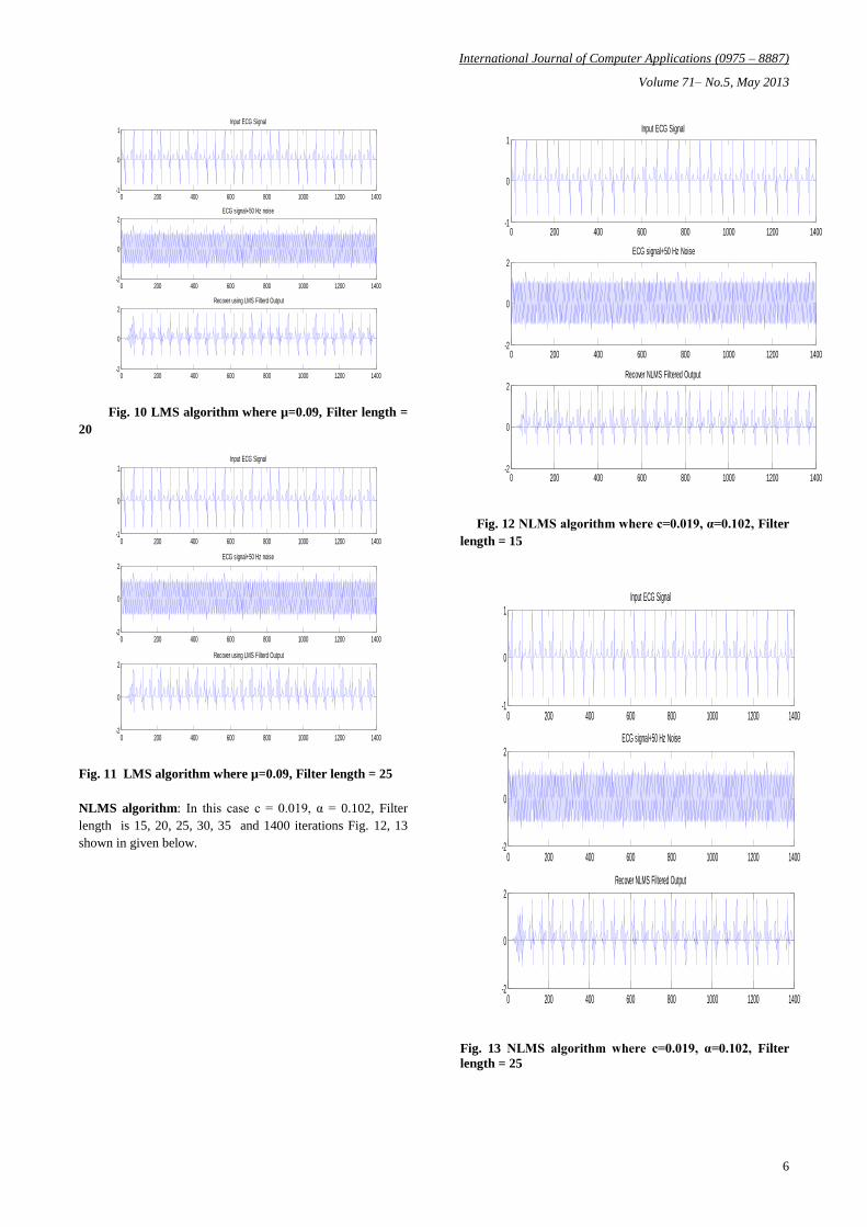
NLMS algorithm: In this case c = 0.019, α = 0.102, Filter

length is 15, 20, 25, 30, 35 and 1400 iterations Fig. 12, 13

shown in given below.

Fig. 12 NLMS algorithm where c=0.019, α=0.102, Filter

length = 15


length = 25

0 200 400 600 800 1000 1200 1400-1

0

1Input ECG Signal

0 200 400 600 800 1000 1200 1400-2

0


0 200 400 600 800 1000 1200 1400-2

0


0 200 400 600 800 1000 1200 1400-1

0

1Input ECG Signal

0 200 400 600 800 1000 1200 1400-2

0


0 200 400 600 800 1000 1200 1400-2

0


0 200 400 600 800 1000 1200 1400-1

0

1Input ECG Signal

0 200 400 600 800 1000 1200 1400-2

0

2 ECG signal+50 Hz Noise

0 200 400 600 800 1000 1200 1400-2

0

2Recover NLMS Filtered Output

0 200 400 600 800 1000 1200 1400-1

0

1Input ECG Signal

0 200 400 600 800 1000 1200 1400-2

0


0 200 400 600 800 1000 1200 1400-2

0




7

NLMS algorithm: In this case c= 0.019, α=0.102, Filter

length is 40 and 1400 iterations in Fig. 14 shown given

below.


length. = 40

The objective was to optimize different adaptive filter

algorithms so that we can reduce interference. In this work,

different Adaptive algorithms were analyzed and compared.

The parameter, LMS step size µ play important role in

determine the convergence speed and stability. Convergence

speed can be controlled by parameter step size µ. I have plot

LMS response for step size µ=0.05 and µ=0.09 with different

filter length 15, 20, 25, 30. I observed that with increased

filter order, accuracy increased and with increased step size

convergence rate took place fast.

These results shows that the LMS algorithm has slow

convergence but simple to implement and gives good results

if step size is chosen correctly and is suitable for stationary

environment. The merits of LMS algorithm is less

consumption of memory and amount of calculation.

The NLMS algorithm changes the step-size according to the

energy of input signals hence it is suitable for both stationary

as well as non-stationary environment. The implementation of

algorithms was successfully achieved for c = 0.019, α = 0.102,

filter length is 15, 20, 25, 40 and 1400 iterations.

The noise cancellation performance of NLMS was observed

consistently better when compared with LMS algorithm.

REFERENCES [1] R.S Khandpur “Biomedical instrumentation hand book),

11th reprint 2008 Tata McGraw –Hill publication

company Limited New Delhi. ISBN-13: 978-0-07-

0473355-3.

[2] Daniel Olguin, Frantz Bouchereau and Sergio Martinez;

“Adaptive notch filter for ECG signals based on the LMS

algorithm with variable step-size parameter” conference

on information sciences and systems, the John Hopkins

University; March 16 –18, 2005.

[3] Plonsey, R. (1996). Electronic Engineer Handbook -

Electrocardiography and Bio-potentials (4th edition),

McGraw-Hill, New York.

[4] M. K. Islam, A. N. M. M. Haque, G. Tangim, T.

Ahammad, and M. R. H. Khondokar , Member, IACSIT

“study and analysis of ecg signal using matlab & labview

as effective tools” International Journal of Computer

and Electrical Engineering, Vol. 4, No. 3, June 2012.

[5] Hon Wan, Rongshen Fu and Li Shi, “The elimination of

50Hz power line interference from ECG using a variable

step size LMS adaptive filtering algorithm”. Life Science

journal, Vol. 3, No. 4, pages 90 – 93. 2006.

[6] Stephen J. chapman “MATLAB programming for

engineers” 3rd Reprint Edition 2003 by Thomson asia Pte

Ltd., Singapore ISBN: 981-240-606-9.

[7] Malindi, P.(2002) “Cancelling power line interference in

electrophysiological signals”. ECT Research Journal, 2.

[8] Widrow B. and Hoff M.E. (1960), “Adaptive switching

circuits”, In IREWESCON Convention Record, pp. 96-

104, New York.

[9] Bernard. Widrow, “Adaptive Noise Cancelling: Principles

and Applications” Proceedings IEEE, vol. 63, pp. 1692-

1716.

[10] Martens S.M.M., Mischi M., Oei, S.G. and Bergmans

J.W.M. (2006), „An improved adaptive power line

interference canceller for electrocardiography‟, IEEE

Transaction on Biomedical Engineering, Vol. 53, pp.

2220-2231.

[11] Zhang Jiashu, Tai Heng-Ming, “Adaptive Noise

Cancellation Algorithm for Speech Processing”, IEEE

Transactions, pp 2489-2492, 2007.

[12] Jafar Ramadhan Mohammed, “A New Simple Adaptive

Noise Cancellation Scheme Based on ALE and NLMS

Filter”, IEEE Transactions, pp 657-662, 2007.

[13] Bertran Eduard, “A Fully Analog Adaptive-Disturbance

Canceller”, IEEE Transactions, pp 1605-1609, 2007.

[14] Bai Lin,Qinye Yin, “A Modified NLMS Algorithm for

Adaptive Noise Cancellation”, IEEE Transactions, pp

3726-3729, 2010.

[15] Mollaei Yaghoub, “Hardware Implementation of

Adaptive Filters”, IEEE Transactions.

[16] Thakor N.V. and Zhu Y.S. (1991), „Applications of

adaptive filtering to ECG analysis: noise cancellation and

arrhythmia detection‟ , IEEE Transaction on Biomedical

Engineering, Vol. 38, No. 8, pp. 785-794.

[17] Ban-Hoe Kwan, Kok-Meng Ong and Paramesran R.

(2005), „Noise removal of ECG signals using legendre

moments‟, 27th Annual International Conference on

Engineering in Medicine and Biology Society, pp. 5627-

5630.

[18] Hae-Jeong Park, Do-Un Jeong and Kwang- Suk Park

(2002), „Automated detection and elimination of periodic

ECG artifacts in EEG using the energy interval

histogram method‟, IEEE Transactions on Biomedical

Engineering, Vol. 49, No. 12, pp. 1526- 1533.

[19] Barbosa P.R.B., Barbosa-Filho J., De Sa C.A.M.,

Barbosa E.C. and Nadal J. (2003), „Reduction of

electromyographic noise in the signal-averaged

electrocardiogram by spectral decomposition‟, IEEE

Transactions on Biomedical Engineering, Vol. 50, No. 1,

pp. 114-117.

[20] G.K. Mithal, Ravi Mittal “Radio Engineering” 19th

Revised Edition Khanna publication company Limited

New Delhi.

[21] S.Salivanhannan, A Vallavaraj,C Gnanapryia , 23rd

reprint 2008, “ Digital signal processing” Tata McGraw

–Hill publication company Limited New Delhi.ISBN-

13:978-0-07-463996-2.

[22] Proakis, J.G. and Manolakis, D.G. (1996) Digital signal

processing 3rd Edition, Prentice Hall.

[23] Jigram H. Shah, Jay M. Joshi, “Digital signal processing”

University science press laxmi publication company

Limited New Delhi.

0 200 400 600 800 1000 1200 1400-1

0

1Input ECG Signal

0 200 400 600 800 1000 1200 1400-2

0


0 200 400 600 800 1000 1200 1400-2

0




8

[24] A. K. Ziarani and A. Konrad, “A nonlinear adaptive

method of elimination of power line interference in ECG

signals,” IEEE Trans. Biomed. Eng., vol. 49, no. 6, pp.

540–547, Jun. 2002.

[25] Suzanna M. M. Martens , Massimo Mischi, S. Guid Oei,

„An Improved Adaptive Power Line Interference

Canceller for Electrocardiography‟ IEEE transactions on

biomedical engineering, vol. 53, no. 11, November 2006.

[26] Syed Zahurul Islam, Syed Zahidul Islam, Razali Jidin,

Mohd. Alauddin Mohd. Ali, “Performance Study of

Adaptive Filtering Algorithms for Noise Cancellation of

ECG Signal”, IEEE 2009.

[27] Mohammad Zia Ur Rahman, Rafi Ahamed Shaik, D V

Rama Koti Reddy, ” Adaptive Noise Removal in the

ECG using the Block LMS Algorithm” IEEE-2009.

[28] Raj Kumar Thenua “Simulation and performance

Analysis of adaptive filter in Noise cancellation”

International Journal of Engineering Science and

Technology Vol. 2(9), 2010, 4373-4378.

[29] A. Srinivasan “Adaptive echo noise elimination for

speech Enhancement of Tamil letter „zha ” , International

Journal of Engineering and Technology Vol.1(3), 2009,

91-97.

[30] Wu Xin, Jeffrey S. Fu, “Side lobe Suppression Using

Adaptive Filtering Techniques”, IEEE Transactions, pp

788-791, 2001.

[31] Abdullah Halim,Yusof Mat lkram, Shah Rizam Mohd

Baki, “Adaptive Noise Cancellation: A Practical Study of

the Least-Mean Square over Recursive Least-Square

Algorithm”, IEEE transactions, pp 448-452, 2002.

[32] Egiazarian Karen and Georgi Iliev, “Adaptive System

for Noise Cancellation in Wireless Communications”,

IEEE Transactions, pp 273-276, 2004.

[33] Jardins T. D. (2002). Cardiopulmonary Anatomy

Physiology (4th ed.).

[34] R.H. Kwong and E.W. Johnston, “A variable step size

LMS algorithm,” IEEE Trans, pp. 1633-1642, 1992.

[35] Mihov, G. (2011) “Subtraction procedure for removing

power line interference from ECG: Dynamic threshold

linearity criterion for interference suppression”. The 4th

Interna- tional Conference on Biomedical Engineering

and Informatics (BMEI), Sofia, 15-17 October 2011.

[36] Aung Soe Khaing and Zaw Min Naing “Quantitative

Investigation of Digital Filters in Electrocardiogram with

Simulated Noises” International Journal of Information

and Electronics Engineering, Vol. 1, No. 3, November

2011.

[37] Aung Soe Khaing and Zaw Min Naing “Quantitative

Investigation of Digital Filters in Electrocardiogram with

Simulated Noises” International Journal of Information

and Electronics Engineering, Vol. 1, No. 3, November

2011.

IJCATM : www.ijcaonline.org

Documents

Designing and Implementation of Algorithms on MATLAB for ...Designing and Implementation of Algorithms on MATLAB for Adaptive Noise Cancellation from ECG Signal Hemant Kumar Gupta