Embed Size (px)
Citation preview

Design Storms
CE 365K Hydraulic Engineering Design
Spring 2015

2
3
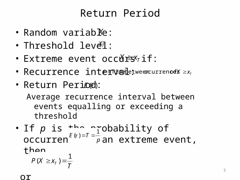
Return Period
• Random variable:• Threshold level:• Extreme event occurs if: • Recurrence interval: • Return Period:
Average recurrence interval between events equalling or exceeding a threshold
• If p is the probability of occurrence of an extreme event, then
or
TxX
Tx
X
TxX of ocurrencesbetween Time
)(E
pTE
1)(
TxXP T
1)(

4
More on return period
• If p is probability of success, then (1-p) is the probability of failure
• Find probability that (X ≥ xT) at least once in N years.
NN
T
TT
T
T
TpyearsNinonceleastatxXP
yearsNallxXPyearsNinonceleastatxXP
pxXP
xXPp
111)1(1)(
)(1)(
)1()(
)(

5
Example• Expected life of culvert = 10 yrs• Acceptable risk of 10 % for the culvert
capacity• Find the design return period
yrsT
T
TR
n
95
11110.0
111
10
What is the chance that the culvert designed for an event of 95 yr return period will have its capacity exceeded at least once in 50 yrs?
41.0
95
111
50
R
R
The chance that the capacity will not be exceeded during the next 50 yrs is 1-0.41 = 0.59

Design Storms
• Get Depth, Duration, Frequency Data for the required location
• Select a return period• Convert Depth-Duration data to a design
hyetograph.

Depth Duration Data to Rainfall Hyetograph

8
TP 40
• Hershfield (1961) developed isohyetal maps of design rainfall and published in TP 40.
• TP 40 – U. S. Weather Bureau technical paper no. 40. Also called precipitation frequency atlas maps or precipitation atlas of the United States.– 30mins to 24hr maps for T = 1 to 100
• Web resources for TP 40 and rainfall frequency maps– http://www.tucson.ars.ag.gov/agwa/rainfall_frequency.ht
ml– http://www.erh.noaa.gov/er/hq/Tp40s.htm– http://hdsc.nws.noaa.gov/hdsc/pfds/

9
2yr-60min precipitation GIS map

10
2yr-60min precipitation map
This map is from HYDRO 35 (another publication from NWS) which supersedes TP 40

An example of precipitation frequency estimates for a location in California
37.4349 N120.6062 W
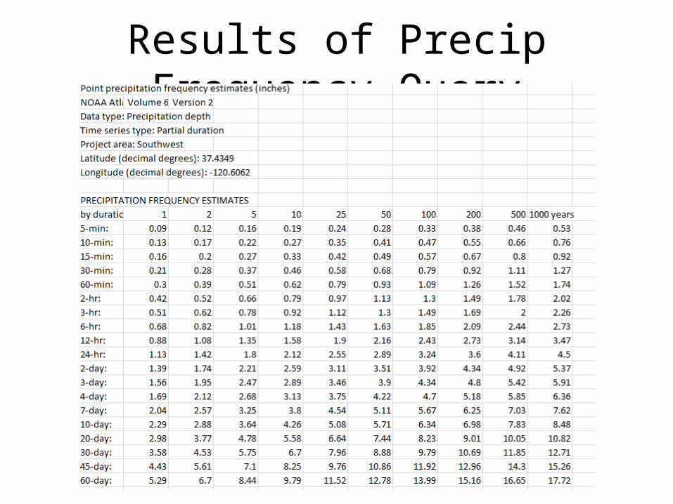
Results of Precip Frequency Query

14
Design areal precipitation
• Point precipitation estimates are extended to develop an average precipitation depth over an area
• Depth-area-duration analysis – Prepare isohyetal maps from point precipitation
for different durations– Determine area contained within each isohyet– Plot average precipitation depth vs. area for each
duration

Tropical Storm Allison

TS Allison

17
Depth-area curve
(World Meteorological Organization, 1983)

TS Allison
1 2 3 4 5 6 7 8 9 10 11 12 13 14 15 16 170
1
2
3
4
5
6
Time (Hours)
Rain
fall
(inch
es)
0 2 4 6 8 10 12 14 16 18 200
5
10
15
20
25
30
Cumulative Rainfall
19
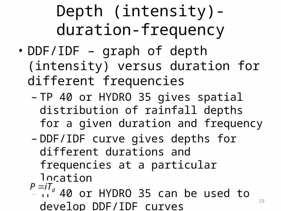
Depth (intensity)-duration-frequency
• DDF/IDF – graph of depth (intensity) versus duration for different frequencies– TP 40 or HYDRO 35 gives spatial distribution of
rainfall depths for a given duration and frequency– DDF/IDF curve gives depths for different durations
and frequencies at a particular location– TP 40 or HYDRO 35 can be used to develop
DDF/IDF curves
• Depth (P) = intensity (i) x duration (Td) diTP

20
IDF curves for Austin
cbt
ai
tscoefficien,,
stormofDuration
intensityrainfalldesign
cba
t
i
Storm Frequency a b c
2-year 106.29 16.81 0.9076
5-year 99.75 16.74 0.8327
10-year 96.84 15.88 0.7952
25-year 111.07 17.23 0.7815
50-year 119.51 17.32 0.7705
100-year 129.03 17.83 0.7625
500-year 160.57 19.64 0.7449
0
2
4
6
8
10
12
14
16
1 10 100 1000
Duration (min)
Inte
nsi
ty (
in/h
r)
2-yr
5-yr
10-yr
25-yr
50-yr
100-yr
500-yr
Source: City of Austin, Watershed Management Division

21
Design Precipitation Hyetographs
• Most often hydrologists are interested in precipitation hyetographs and not just the peak estimates.
• Techniques for developing design precipitation hyetographs
1. SCS method2. Triangular hyetograph method3. Using IDF relationships (Alternating block method)

TS Allison
1 2 3 4 5 6 7 8 9 10 11 12 13 14 15 16 170
1
2
3
4
5
6
Time (Hours)
Rain
fall
(inch
es)

23
SCS MethodSCS (1973) adopted method similar to DDF to develop dimensionless rainfall temporal patterns called type curves for four different regions in the US.SCS type curves are in the form of percentage mass (cumulative) curves based on 24-hr rainfall of the desired frequency.If a single precipitation depth of desired frequency is known, the SCS type curve is rescaled (multiplied by the known number) to get the time distribution. For durations less than 24 hr, the steepest part of the type curve for required duraction is used
24
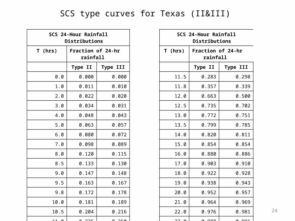
SCS type curves for Texas (II&III)
SCS 24-Hour Rainfall Distributions SCS 24-Hour Rainfall Distributions
T (hrs) Fraction of 24-hr rainfall T (hrs) Fraction of 24-hr rainfall
Type II Type III Type II Type III
0.0 0.000 0.000 11.5 0.283 0.298
1.0 0.011 0.010 11.8 0.357 0.339
2.0 0.022 0.020 12.0 0.663 0.500
3.0 0.034 0.031 12.5 0.735 0.702
4.0 0.048 0.043 13.0 0.772 0.751
5.0 0.063 0.057 13.5 0.799 0.785
6.0 0.080 0.072 14.0 0.820 0.811
7.0 0.098 0.089 15.0 0.854 0.854
8.0 0.120 0.115 16.0 0.880 0.886
8.5 0.133 0.130 17.0 0.903 0.910
9.0 0.147 0.148 18.0 0.922 0.928
9.5 0.163 0.167 19.0 0.938 0.943
9.8 0.172 0.178 20.0 0.952 0.957
10.0 0.181 0.189 21.0 0.964 0.969
10.5 0.204 0.216 22.0 0.976 0.981
11.0 0.235 0.250 23.0 0.988 0.991
24.0 1.000 1.000

25
Alternating block method• Given Td and T/frequency, develop a hyetograph in
Dt increments1. Using T, find i for Dt, 2Dt, 3Dt,…nDt using the IDF curve
for the specified location2. Using i compute P for Dt, 2Dt, 3Dt,…nDt. This gives
cumulative P.3. Compute incremental precipitation from cumulative P.4. Pick the highest incremental precipitation (maximum
block) and place it in the middle of the hyetograph. Pick the second highest block and place it to the right of the maximum block, pick the third highest block and place it to the left of the maximum block, pick the fourth highest block and place it to the right of the maximum block (after second block), and so on until the last block.

26
Cumulative Incremental Duration Intensity Depth Depth Time Precip (min) (in/hr) (in) (in) (min) (in) 10 4.158 0.693 0.693 0-10 0.024 20 3.002 1.001 0.308 10-20 0.033 30 2.357 1.178 0.178 20-30 0.050 40 1.943 1.296 0.117 30-40 0.084 50 1.655 1.379 0.084 40-50 0.178 60 1.443 1.443 0.063 50-60 0.693 70 1.279 1.492 0.050 60-70 0.308 80 1.149 1.533 0.040 70-80 0.117 90 1.044 1.566 0.033 80-90 0.063 100 0.956 1.594 0.028 90-100 0.040 110 0.883 1.618 0.024 100-110 0.028 120 0.820 1.639 0.021 110-120 0.021
Example: Alternating Block Method
90.13
6.9697.0
d
ed TfT
ci
tscoefficien,,
stormofDuration
intensityrainfalldesign
fec
T
i
d
0.0
0.1
0.2
0.3
0.4
0.5
0.6
0.7
0.8
0-10 10-20 20-30 30-40 40-50 50-60 60-70 70-80 80-90 90-100
100-110
110-120
Time (min)
Pre
cip
itat
ion
(in
)
Find: Design precipitation hyetograph for a 2-hour storm (in 10 minute increments) in Denver with a 10-year return period 10-minute