DESIGN, SETUP OF AN OPTICALLY ACCESSIBLE INTERNAL COMBUSTION ENGINE

FOR STUDY OF GASOLINE DIRECT INJECTION COMBUSTION

BY

ROBERT M. DONAHUE

THESIS

Submitted in partial fulfillment of the requirements

for the degree of Master of Science in Mechanical Engineering

in the Graduate College of the

University of Illinois at Urbana-Champaign, 2017

Urbana, Illinois

Adviser:

Professor Chia-fon F. Lee

ii

Abstract

Gasoline direct injection (GDI) engines are becoming attractive options for automobiles.

The precise control over fuel delivery increases the potential for better fuel efficiency and higher

performance. In this study, a single-cylinder optically-accessible engine was built to visualize

GDI combustion. The optical engine was originally designed and used as a compression ignition

engine for study of diesel combustion, but was extensively modified for GDI. The cylinder head

was modified to include a spark plug, and a new ignition system was designed. In addition, a

lowered compression ratio, new piston geometry, and new fuel injector were employed.

In the experiment, combustion of a 20 percent ethanol/80 percent pure 90-octane gasoline

fuel blend was studied. Experiments were conducted at 1200 rpm, and intake air and fuel were

independently controlled. A metal version of the optical piston was made, and preliminary tests

were conducted using the metal configuration. From these tests, engine performance, stability,

and emissions were measured. Following the metal engine testing, an optical study was

performed. Using a high-speed camera at 12,000 frames per second, images of fuel injector

spray as well as combustion were recorded. A 3-dimensional Mie scattering technique was used

to image the interaction of the fuel spray with the piston and cylinder walls, and natural flame

luminosity was used to capture combustion images.

From the experiments, it was concluded that in this configuration, a double injection with

a first injection timing of 180° BTDC and a 90 percent/10 percent first/second injection split

gave the best results with respect to engine stability and emissions. The combustion and spray

imaging paired with corresponding performance and emissions data provide a broad picture of

GDI combustion characteristics.

iii

Acknowledgements

Firstly, I would like to sincerely thank my research advisor, Professor Chia-fon Lee, for

the many opportunities that were provided to me as a graduate student at Illinois. The projects I

have worked on under his guidance have been of the most stimulating and challenging

engineering tasks I have faced in my life. The time I have spent here has made me a better

engineer and person.

I would like to thank my good friend and colleague, Karthik Nithyanandan, for being a

great partner in crime throughout my time in graduate school. He taught me everything I know

about IC engines and kept me sane during many late nights spent working in the lab. We have

made a great team.

A special thanks goes to Cliff Gulyash and everyone else in the MechSE Machine Shop.

They were able to take my wildest ideas and make them a reality. I would also like to thank

Laurie Macadam for constant help to keep my projects well supplied, always with a smile.

I would like to thank the Randys for making the last two years the best of my life.

Together, we managed to infuse so much fun and vitality into the daily grind.

I would like to give thanks to my loving family. My parents, Mike and Carol Donahue,

have guided me down a path of opportunity and always allowed and encouraged me to pursue

my passions. Finally, Rachel Mileski, my girlfriend of eight years, has provided endless love,

support, and encouragement through all of the ups and downs of life, for which I thank you.

iv

Table of Contents Page

Chapter 1: Introduction .............................................................................................................. 1

1.1 Background ...................................................................................................................... 1

1.2 Literature Review ............................................................................................................. 3

1.3 Tables & Figures .............................................................................................................. 6

Chapter 2: DIATA Optical Engine Setup .................................................................................. 9

2.1 Optical Engine Design ..................................................................................................... 9

2.2 Engine Modifications for GDI ....................................................................................... 12

2.3 Engine Subsystems ......................................................................................................... 16

2.4 Engine Controls .............................................................................................................. 20

2.5 Data Acquisition ............................................................................................................. 22

2.6 Tables & Figures ............................................................................................................ 28

Chapter 3: Experimental Procedure ......................................................................................... 42

3.1 Equipment Calibration ................................................................................................... 42

3.2 Metal Engine Operation ................................................................................................. 43

3.3 Optical Engine Operation ............................................................................................... 44

Chapter 4: Results & Discussion .............................................................................................. 47

4.1 Metal Engine Results ..................................................................................................... 47

4.2 Optical Engine Results ................................................................................................... 51

4.3 Tables & Figures ............................................................................................................ 55

Chapter 5: Conclusions ............................................................................................................ 72

References ..................................................................................................................................... 74

Appendix A: Troubleshooting ...................................................................................................... 76

Appendix B: Engine Startup Checklist ........................................................................................ 78

1

Chapter 1: Introduction

1.1 Background

Internal combustion (IC) engines are an integral part of the automotive and transportation

industries, and will continue to be for decades to come. In 2015, 98.1 percent of passenger cars

and light trucks in the United States were driven by either gasoline, diesel, or flex-fuel/ethanol

burning internal combustion engines. The U.S. Energy Information Agency predicts that by the

year 2050, that number will drop to 85.5 percent. However, the EIA predicts that the total

number of cars and light trucks on the road will increase by 23 percent from 240 million in 2015

to 295 million in 2050, so the number of IC engines on the road will actually increase by

approximately 17 million over the next three decades [1].

Several advantages of IC engines exist. Firstly, it is a technology that has been improved

and refined for over 200 years, so it provides reliable, low cost transportation to millions of

people. In addition, infrastructure in the United States and around the world is well established,

so keeping gasoline or diesel engines fueled and on the road has become second nature.

However, growing concerns regarding the environmental impact of IC engines have accelerated

the implementation of increasingly stringent emissions regulations. For that reason, significant

research is being conducted to try to improve IC engine performance, while lowering fuel

consumption and harmful emissions.

Over the past 25 years, fuel economy has increased significantly. In 1980, the average

fuel economy for a new passenger car was 24 mpg, and by 2014 it had increased by 50 percent to

36 mpg [2]. Standards for fuel economy, as well as particulate, soot, and CO emissions are only

accelerating, which is pushing advancement in the IC engine research community and industry

alike.

2

One rapidly growing strategy to increase the fuel efficiency for gasoline engines is using

gasoline direct injection (GDI). The first commercially available GDI powered vehicle was the

Mitsubishi Galant in 1996. In 2008, 2.3 percent of new vehicles used GDI, which had increased

to over 45 percent by 2015 [3]. GDI is a method in which a high-pressure fuel system injects

fuel directly into the combustion chamber during the intake or compression stroke. The

alternative, called port fuel injection (PFI), is a method in which gasoline is injected into the

intake port, and a premixed charge is drawn into the chamber through the intake valve. GDI has

several advantages over PFI. Firstly, GDI allows direct control of when and how much fuel is

injected. An earlier injection creates a more uniform premixed charge, similar to PFI, while a

later injection can create stratification. In addition, when the injected fuel vaporizes, the charge

is cooled, allowing higher compression ratios, which lead to greater work output from the

engine.

The main drawback to GDI engines is the cost of the fuel supply system. The injection

pressure for GDI must be significantly higher because the charge is injected into the chamber

when the intake air is already compressed, whereas PFI injectors must only overcome near-

atmospheric pressures. Also, with a more complex fuel delivery system comes increased need

for maintenance, however new injection systems are more reliable than ever.

In the present study, GDI combustion of a 20 percent ethanol 80 percent gasoline blend is

studied in an optically-accessible internal combustion engine. The fuel spray and combustion are

observed from below the combustion chamber through a transparent piston and from the side

through an optical window in the cylinder liner. Different injection strategies as well as lean

combustion are studied optically, and corresponding performance and emissions data are

gathered.

3

1.2 Literature Review

An optically accessible engine is a unique piece of diagnostic equipment for studying

combustion, as it can give an otherwise inaccessible look at the spray and combustion

characteristics inside of an IC engine. Several types of optical access are possible through side

windows, transparent cylinder liners, transparent pistons, and/or endoscopes. Typical optical

engine investigations study spray penetration and interactions, combustion evolution, or both.

Due to the unconventional nature of optical engines, they are typically one-off designs and can

have vastly different features. Optical engines are particularly useful for GDI research due to the

unique combustion effects from stratification and multiple injections.

In a study by Guo, et al. [4], a single-cylinder optically-accessible engine was used to

study flash boiling injector spray. This optical engine had a fully transparent cylinder liner as

well as a flat transparent piston top. A pneumatic configuration allowed for assembly and

disassembly of the transparent liner in order to easily clean the optical components. The

transparent liner allowed phase Doppler anemometry (PDA) to be used to analyze fuel droplet

size and velocity. In addition, a 45-degree mirror placed below the piston top allowed high

speed bottom-view photography of the injector spray using a high-speed camera and an LED

light source. A schematic of the setup is shown in Figure 1.1. GDI spray was studied at an

engine speed of 1200 rpm at different fuel temperatures to determine the effect on flash boiling

and spray evolution. It was found that as fuel temperature rose, the Sauter mean diameter (SMD)

of the spray droplets decreased steadily.

In a similar work by Song and Park [5], the effect of injection strategy on GDI injector

spray development was studied in a single-cylinder optical engine. This optical engine had a

quartz window in the cylinder to observe the side view of the injector spray. Spray images were

4

taken at 10 kHz using a high-speed camera and a metal halide lamp for illumination. A basic

schematic of the setup is shown in Figure 1.2. From this study, it was concluded that higher

injection pressures created smaller fuel droplets, allowing the intake flow to mix with the fuel

more easily, creating a more homogeneous mixture.

In addition to GDI spray investigation, several studies have been conducted to observe

GDI combustion using an optical engine. In one such study by Catapano et al. [6], the effect of

different ethanol blends on combustion and soot formation was studied using natural luminosity

imaging and spectroscopy. The single-cylinder optical engine was equipped with a flat sapphire

piston top, and the top section of the cylinder liner was a quartz ring. A hollow piston extension

with a 45° mirror was used to gain optical access from the bottom. A schematic of the setup is

shown in Figure 1.3. Two separate high speed cameras were used, and synchronized by the shaft

encoder. The first had a range in the visible spectrum and was used to capture natural flame

luminosity images. The second was an intensified charge coupled device (ICCD) with a 200 –

800 nm range that captured visible and UV emissions. From the study, it was observed that the

presumed soot radiance from the natural luminosity images agreed with the emission spectra

captured by the ICCD. These results were corroborated by the soot particle size distribution

captured in the exhaust. It was also found that at full load, soot quantity was reduced with

increasing ethanol percentage.

In a second study by Catapano et al. [7], a different GDI optical engine was used to study

combustion of ethanol blends. This turbocharged, four-cylinder engine was modified with piston

and cylinder extensions in which a 45-degree mirror was placed. The piston top was made from

transparent quartz. An endoscopic probe was inserted into the chamber through the cylinder

head, and was attached to an ICCD high-speed camera. The endoscope had a 70-degree field of

5

view that was angled 30 degrees below horizontal to capture a cross section of the combustion

chamber. A schematic of the setup can be seen in Figure 1.4. The camera was used to

photograph the spray evolution and combustion evolution. From this study, it was concluded

that increasing ethanol blend ratio improved IMEP and combustion stability. Spray structure

was found to change greatly with varying ethanol blend ratio due to effects of flash boiling.

A paper by Dahlander and Hemdal [8] studies the effect of different triple injection

strategies on GDI combustion in a single-cylinder optical engine. This engine is similar to the

one described in reference [6] with a quartz upper cylinder liner. The cylinder head has pentroof

construction, with triangular pentroof windows to observe the side view spray. In addition, there

is an optical window in the piston to visualize combustion from below. A picture of the optical

engine setup is shown in Figure 1.5. Two high speed cameras were used to simultaneously

capture the side and bottom view images. The side view camera was black and white, and it was

used to distinguish between bulk combustion, pool fires, and jet flames. The bottom view

camera was a color camera, and it was used to differentiate between emission species. Blue

flame is typically dominated by CH radicals, while the yellow flame is predominantly from soot

luminescence. In this study, many different triple injection strategies were tested. It was

concluded that when the bulk of the fuel was injected closer to spark timing, increased

stratification led to better combustion stability and performance, but higher soot formation.

Earlier injections led to less soot, but also decreased work output and increased penetration,

which led to cylinder wall impingement.

In the present study, a single-cylinder optical engine was built to further study GDI

combustion of ethanol blends. An extended optical piston as well as a quartz side view window

allow simultaneous side and bottom view combustion and spray visualization. A creative optics

6

setup allows both views to be captured using a single high speed camera. Corresponding

emissions and performance data help to further interpret the optical images and provide new

insights into GDI combustion regimes.

1.3 Tables & Figures

Figure 1.1: Single-cylinder optical engine with transparent liner and flat optical piston top [4]

7

Figure 1.2: Optical engine configuration (right) with transparent window for spray imaging [5]

Figure 1.3: Single-cylinder optical engine with transparent liner section and flat optical piston

top [6]

8

Figure 1.4: Four-cylinder optical engine with quartz piston and endoscope [7]

Figure 1.5: Single-cylinder optical engine with pentroof side windows and quartz piston [8]

9

Chapter 2: DIATA Optical Engine Setup

2.1 Optical Engine Design

The optical engine was built from a single-cylinder DIATA (Direct Injection Aluminum

Through-bolt Assembly) diesel research engine supplied by Ford Motor Company. Then engine

retains all of the original geometry of the ports and combustion chamber, except for a new piston

design. The piston geometry was optimized using computation specifically for gasoline direct

injection research. The engine has a displacement volume of 300 cubic centimeters. The

cylinder head is all aluminum, and the head and optical extension are built onto an FEV

crankcase. The cylinder head has a flat roof and contains four valves, two intake and two

exhaust. The valves are actuated by dual overhead camshafts. Roller-type cam follower rocker

arms sit atop hydraulic tappets to maintain zero valve clearance when the engine is operating.

General engine specifications are listed in Table 2.1.

For optical access, several modifications were made to the original DIATA prototype

engine. Firstly, to allow imaging from below the combustion chamber, an optical piston was

made using two-part construction. The piston top was made from Corning 7980 fused silica.

This material has high transmissivity into ultraviolet wavelengths, as well as having elevated

tensile and compressive strength compared to other types of silica. The fused silica piston top

was manufactured by Pacific Quartz. The silica piston top mounted into an Invar 36 metal

sleeve using a three-lobed locking ring and Duralco 4525 high temperature epoxy. The locking

ring was epoxied into a groove on the silica piston top, and the ring’s three lobes slid into three

corresponding grooves on the Invar sleeve. The piston and lock ring were then rotated, fixing

the piston in place. The Invar sleeve served as an adapter to bolt the silica piston to the

aluminum piston extension. It also provided grooves for the piston rings. Invar 36 is a 36

10

percent nickel-iron alloy, chosen because it has a low thermal expansion coefficient that close to

fused silica.

A metal piston of equivalent geometry was also made. The metal piston allowed greater

durability for testing the engine before the optical piston was installed. Like the optical piston,

the metal piston was made with two-part construction: an aluminum piston top fit into a stainless

steel piston sleeve. The piston top was machined from 2024-T4 aluminum because of its

relatively low thermal expansion coefficient. The piston was machined such that the mass was

the same as the optical piston, so no balancing issues occurred. The machined aluminum piston

top bolted into the stainless-steel piston sleeve, and the sleeve bolted to the extension. The two-

part design made it easier to experiment with the metal piston geometry without having to re-

machine the rings and mounting points each time, and the greater density of the stainless-steel

sleeve allowed the metal piston to be equally as heavy as its optical counterpart.

Special oil-less piston rings were used with the optical engine, as any lubrication on the

optical components would have caused images to become obstructed. There were two sealing

rings and one rider ring. The sealing rings were two-piece step-cut expanding rings, and were

used to seal the gases in the chamber. The rider ring was an angle cut ring that sat below the

sealing rings and was used to support the piston, not for sealing. The inner expander ring for the

sealing rings was made from stainless steel. Two different materials were used for the outer step

cut sealing rings. Originally, Vespel SP-21 was used, however when new rings were purchased,

TrueTech 3210 bronze powder-filled PTFE was used. Both of these materials have high wear

and temperature resistances. Vespel SP-21 is superior in both properties, however the TT3210 is

much less expensive for a slight decrease in temperature resistance. After testing both types of

rings in the engine, the Vespel SP-21 rings indeed showed less sign of wear, however the

11

TT3210 rings held up suitably for our needs. The rider ring was made from a carbon-filled

PTFE. All rings were manufactured by Cook Compression.

The piston sleeve was mounted atop a Bowditch-type piston extension, made from 2024-

T4 aluminum alloy, which mounted to the top of the original piston in the crankcase. This

extension was hollow with slots cut along two sides, allowing a 45-degree mirror to be installed

inside the piston extension, shown in Figure 2.1. This mirror allowed access for laser diagnostics

and images to be taken from below the piston. The cylinder head was raised above the crankcase

by four machined 304-stainless-steel rods.

Just below the cylinder head and above the drop-down cylinder liner was a machined

window spacer, made from 304 stainless steel. This spacer had four pockets that surround the

combustion chamber that could house either a fused silica window, or a 304-stainless-steel

window blank. The inside wall of the windows was rounded to match the contour of the cylinder

walls, shown in Figure 2.2. To seal the windows into the pockets, Momentive RTV60, a high-

temperature silicone compound, was used in conjunction with Momentive SS4004P primer. This

prevented leakage around the windows, as well as held the window in place. It is imperative to

use the primer, as the RTV does not adhere to the stainless steel or silica on its own, and

windows can be drawn into the cylinder on the intake stroke. If this happens, the piston will

collide with the window on the upward stroke and cause major damage to the engine.

Below the window spacer, a drop-down cylinder liner surrounded the piston and

extension, and could be lowered to allow easy access to clean the optical piston. The liner mated

with the window spacer, and proper alignment was ensured by angled mating surfaces. An O-

ring sealed the liner to prevent leakage, and the mating surfaces were pressed together using a

hydraulic system. The hydraulic system consisted of a lifter that was below the piston extension,

12

a hydraulic fluid reservoir, and pressurized nitrogen. The nitrogen was pressurized to 30 psi,

forcing the hydraulic fluid to press the liner against the window spacer. The engine must not be

run without the hydraulic system pressurized or it will be damaged. A full schematic of the

optical engine is shown in Figure 2.3, and the engine is shown in Figure 2.4. Further information

about this engine can be found in reference [9].

2.2 Engine Modifications for GDI

2.2.1 Cylinder Head Modification

The single-cylinder DIATA research engine was originally a compression ignition diesel

engine. In order to use this engine for GDI research, several modifications needed to be made,

most important of which was the addition of an ignition system. The obvious choice was to

introduce a spark plug into the cylinder head, however, space was quite limited. A three-

dimensional CAD model was created using the original engine drawings, allowing for easy

visualization of the internals of the cylinder head. Due to the existing coolant and oil passages,

as well as intake, exhaust, and fuel injector, there existed only one feasible region in the head for

the spark plug hole to be machined. It was determined that the hole would be between the

exhaust runner and the in-cylinder pressure transducer, at such an angle not to interfere with two

cooling passages and the hydraulic lifters.

A typical gasoline engine of this size generally uses a spark plug with an M10 thread, and

requires a 5/8" socket with an outer diameter of 7/8" (~22 mm) to install. The distance between

the valves where the plug would protrude into the cylinder was just 10 mm, and the maximum

diameter hole that could be safely drilled into the cylinder head without causing interference with

existing passages and leaving sufficient material was determined to be just 13 mm. As such, a

smaller spark plug solution was necessary. After much research, it was determined that the

13

smallest commercially available spark plug that could withstand the necessary temperatures and

provide sufficient energy was the NGK ER9EH plug. The ER9EH is a resistive copper core plug

with a heat range value of nine. The thread size was 8 mm, allowing it to fit just between the

valves in the cylinder head. However, the hex size was 13 mm, meaning it would not be possible

to use a socket to install the plug.

To counter this issue, the spark plug was modified to make installation possible. The

plug was put into a lathe, and the hex was turned down, leaving an outer diameter of 12 mm.

The plug was then placed into a mill vertically, and four slots were drilled into the body of the

plug. An installation tool was made with four prongs corresponding to the slots in the plug, and

an 11-mm hex was machined in the top of the tool so the plug could be tightened using a wrench.

The modified spark plug and installation tool are shown in Figure 2.5.

Since the engine was to be used for gasoline direct injection combustion, the precise

location of the plug was very important. For this engine design, it was important for the spark

plug to be as close to the fuel injector as possible, to protrude into the center bowl of the piston,

and not to interfere with any existing features. Using an iterative approach, the precise location

was determined within the specified region of the cylinder head. It was decided that the tip of

the spark plug would be halfway between the intake and exhaust valves on the exhaust side of

the cylinder head, and 11.5 mm from the fuel injector tip. The axis of the spark plug hole was

made to be at a compound angle. From the top view, the axis of the spark plug lay in a plane six

degrees off of perpendicular. Within that plane, the axis was 38 degrees off of vertical. Figure

2.6 shows the CAD model of the spark plug within the cylinder head. The spark plug hole was

milled in a three-axis Trak K3 milling machine by the University of Illinois Department of

Mechanical Science and Engineering machine shop. Specific tooling and very precise setup was

14

required to align the compound angle correctly. Figure 2.7 shows the cylinder head mounted in

the mill for machining. Figure 2.8 shows the spark plug installed into the cylinder head.

2.2.2 Spark Plug System

In addition to adding a spark plug, a system to fire the plug and properly time it with the

crankshaft was necessary to convert the engine from diesel to GDI. A spark circuit was designed

using a VB921ZVFI ignition coil driver. This chip is a monolithic integrated circuit that

combines vertical current flow with a coil current limiting circuit and collector voltage clamping.

It was specifically designed for high performance electronic vehicle ignition systems. It is

essentially an electronic method of emulating a points system. The circuit was originally

coupled with just an MSD Blaster 2 ignition coil, as shown in the circuit diagram in Figure 2.9.

However, after troubleshooting this setup, it was determined that while the spark fired

outside of the engine, the spark energy was not sufficient to arc under compression. To try to

solve this issue, two further iterations of the spark circuit were attempted. The first kept the

original circuit intact, and added an MSD Digital 6A Ignition Control box, shown in Figure 2.10.

This circuit greatly increased spark energy, and allowed the engine to fire. However, the

electromagnetic interference emitted by the box caused other parts of the data acquisition system

to malfunction. To try to solve this, a higher-grade spark plug wire and additional EMI shielding

were used, however the EMI remained an issue and it was decided to no longer use the MSD

box.

The third iteration of the spark circuit again retained the original VB921ZVFI circuit, and

added a new Dynatek DBR-1 ignition booster box that was specifically designed for an engine

with one ignition coil such as ours. This circuit proved to be the final solution, as it allowed the

15

engine to fire properly, and did not interfere with the data acquisition. It is shown in Figure 2.11.

The spark system is controlled using LabVIEW, and is further discussed in Section 2.4.2.

2.2.3 Piston & Compression Ratio Modification

Another significant modification to the DIATA engine was changing the piston and

compression ratio. The new piston geometry was a novel two-zone piston, which was designed

and optimized by the UIUC computational team. The original diesel engine had a compression

ratio of 19.1:1, however the target compression ratio for the new piston design was 16:1. To

properly adjust the compression ratio, it was necessary for the proper squish height to be set,

which could be changed by adding or removing material from the piston sleeve. To calculate

this height, the clearance volume was divided into three zones, Vcrevice, Vsquish, and Vbowl, shown in

Figure 2.12. The following equations outline the process for solving for the squish height, h.

The total clearance volume desired was determined by the compression ratio, using the following

formula and the desired compression ratio of 16:1.

The crevice volume was known from the diameter of the piston, D, the bore, B, and the height

between the piston top and first ring, R. The bowl volume was known from the CAD model of

the piston, and for the calculation, it included any irregularities in the flat roof of the cylinder

head. It was found that the appropriate squish height was 2.18 mm, and the piston sleeve was

modified accordingly.

16

2.2.4 Miscellaneous Modifications

A few other minor modifications were made to the DIATA engine in order to perform

gasoline direct injection research. The original diesel fuel injector fit into a threaded sleeve that

screwed into the cylinder head, allowing injector orientation to be rotated about its axis. The

injector slid into this sleeve, and was held in place by a rounded retaining ring. The new

injectors used for GDI combustion had slightly different geometry. A new sleeve was designed,

maintaining the geometry of the outer threads, so it could screw into the same hole in the

cylinder head. The inner diameter and height of the sleeve were changed to accommodate the

new injector geometry. The new injectors were then modified to incorporate a rectangular snap

ring groove to fit just below the sleeve, and a custom snap ring was machined from heat treated

spring steel. The injector and sleeve assembly is shown in Figure 2.13.

In addition, some repairs and improvements were made to the DIATA engine. The

tapped bolt holes in the cylinder head where the exhaust manifold mounted were stripped, so

Heli-Coil threaded inserts were added. The oil fittings supplying oil to the cylinder head and

valve train were a standard thread, sealed with a gasket, and the fittings were broken and leaky.

A new, NPT-type fitting was determined to be a better choice, so the head was modified to

incorporate the new oil lines. The original mount for the 45-degree mirror was no longer

available, so a new 45-degree mirror mount was designed and made to fit below the piston in the

optical engine.

2.3 Engine Subsystems

2.3.1 Fuel Supply

Fuel was supplied using a non-return loop system. A fuel reservoir canister was made

from 1 1/2" schedule-40 stainless-steel pipe, enclosed with stainless steel caps on each end.

17

Each cap contained a female NPT fitting to connect to the ¼" stainless steel tubing used as fuel

line. The fuel canister was pressurized using an S.J. Smith SJ6000 485 cubic foot, 6000 psi

nitrogen bottle. A 6000 psi Smith regulator was used to control fuel pressure up to 4000 psi.

Typical injection pressure was 2900 psi (200 bar). A Norman Filter Company 4323GG-10VN

high-pressure inline filter was used between the fuel canister and fuel injector. A separate

canister was used to capture excess fuel from the fuel return line. A schematic of the fuel supply

system is shown in Figure 2.14.

Two different fuel injectors were used for this research. The first was a prototype

injector designed by our computational team to work with the new piston bowl geometry. The

second was a commercially available Delphi GDI fuel injector. Both injectors were solenoid

actuated, and they were controlled using an in-house injector driver. The driver could provide up

to three injections per cycle. Further details of the driver and control system can be found in

Section 2.4.2. The fuels used in this study was a gasoline-ethanol blend comprised of 20 percent

ethanol and 80 percent pure gasoline. To prevent wear on the injectors, Stanadyne Diesel Fuel

Lubricity Additive was added to the blend at a ratio of 1 part additive to 1000 parts fuel.

2.3.2 Air Supply

A regulated supply of air was supplied to the DIATA intake manifold, and the pressure

could be set above or below atmospheric conditions to simulate boosted or throttled conditions.

The air originated from the building air supply, compressed by an Ingersoll Rand SSR XF650 to

pressures ranging from 90 to 100 psi. A heavy-duty regulator then reduced the pressure to 50

psi, and reduced the pressure fluctuations. Once in the lab, a Valtek Mark 1 pressure controller

was used to set the intake pressure between 10 and 40 psi with a maximum flow rate of 260

SCFM. The air then passed through an Ogden ACK5A air heater. In the GDI experiments, the

18

heater was not used, and air temperature was maintained at 23° C. After the heater, the air

entered a seven-gallon surge tank made by Brunner Engineering and Manufacturing. This

further reduced pressure fluctuations, as the volume of the surge tank was much larger than the

displacement volume of the engine. From the surge tank, the air flowed through two intake

runners, one for each intake valve. Each runner was fitted with a ball valve to control swirl

characteristics in the cylinder. The gases exited the chamber through two exhaust valves into a

single exhaust runner into the building exhaust.

Intake pressure was controlled using a separate computer with a PID LabView program.

The intake pressure was measured in the surge tank using a Setra 280E pressure transducer.

Based on the intake pressure measurement and the pressure set point, LabView provided an

output signal of 4 to 20 mA to the Valtek pressure controller.

The mass air flow into the chamber was measured through a Lambda Square orifice plate,

in conjunction with two pressure transducers. A Honeywell 142PC15D differential pressure

transducer measured the differential pressure across the orifice plate, and an Omega PX303-

100G5V pressure transducer measured the pressure on the high side of the orifice plate. Using

these three, as well as a thermocouple to measure air temperature, the mass flow rate was

calculated by a LabView program. A schematic of the air supply system can be found in Figure

2.15. Figure 2.15 through Figure 2.18 have been modified and adapted to reflect the current

engine systems, and the original figures can be found in the Master’s Thesis by Tien Mun Foong

[10].

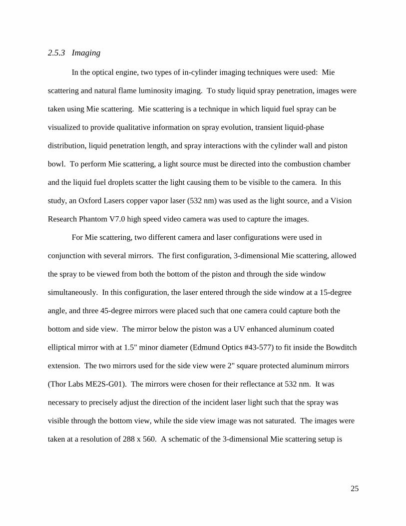
2.3.3 Cooling

To prevent all possible parasitic loads on the optical engine, the cooling and lubrication

systems were stand-alone systems driven by external electric pumps. The cooling system was a

19

closed-loop system consisting of a coolant reservoir, a water pump, and a tube-in-shell heat

exchanger. The coolant fluid used consisted primarily of building water, mixed with Caterpillar

SCA 3P-2044 coolant additive. The additive was mixed in at a ratio of 6% by volume, and it

prevented rust and scale deposits from forming in the cooling system. The coolant was kept in a

five-gallon stainless steel reservoir, which contained a Chromalox ARMTS-3305T2 coolant

heater that was submerged in the coolant. The coolant was circulated through the engine while it

was heated to 80° C to pre-heat the engine to operating conditions without having to run the

engine for an extended period of time. From the reservoir, an electric Leeson C6C34FK61A

pump pumped the coolant into the engine. The coolant flowed in parallel through three separate

loops in the engine. One loop was through the crank case, one through the cylinder liner, and

one through the cylinder head. After exiting the engine, the coolant flowed through a tube-in-

shell liquid-liquid heat exchanger that was cooled using building water. A Johnson Controls

T8000 thermostat valve was used to regulate the flow of building water. When the temperature

exceeded 80° C, the thermostat opened allowing cool water to flow into the shell of the heat

exchanger. From the heat exchanger, the coolant traveled back to the reservoir. There are two

thermocouples that monitored coolant temperature before and after the heat exchanger. A

detailed schematic of the cooling system can be found in Figure 2.16.

2.3.4 Lubrication

The lubrication system for the DIATA was a closed loop system similar to the cooling

system, consisting of an oil reservoir, an oil pump, a tube-in-shell heat exchanger, and an oil

sump pump. The oil typically used was synthetic SAE 15W-40 engine oil. Like the coolant, the

oil was kept in a five-gallon stainless steel reservoir, and was preheated using a Chromalox

ARMT0-2155T2 heater. The oil was circulated through the engine while it was preheated to 70°

20

C to simulate the operating oil temperature of an engine at steady state. The oil was pumped

from the reservoir using a Grundfos C-4J514565-P1-9825 pressure pump, passing through an in-

line HYDAC International 0160MA010P oil filter. From the filter, the oil passed through a tube-

in-shell heat exchanger that was controlled using a Johnson Controls T8000 thermostat in the

same way as the coolant heat exchanger. There are two thermocouples that monitored oil

temperature before and after the heat exchanger. The oil then entered the engine in several

different locations. The first was into the crank case where the main bearings and connecting

rods are lubricated. The next was through four separate passages into the cylinder head, where

the hydraulic lifters are pressurized. The final entry point was into the cam housing where the

cam bearings are lubricated. The oil from the cam housing and the cylinder head drained

through a common tube into the crank case. A Leeson C6C34FK36C sump pump then pumped

the oil from the crank case back into the oil reservoir. While the pressure pump ran

continuously, the sump pump only ran periodically when the oil needed to be drained from the

crank case. This was controlled by an oil level sensor in the reservoir, only turning on the sump

pump when the level dropped too low. Oil pressure was monitored using LabView in

conjunction with an Omega PX303 pressure transducer. A detailed schematic of the lubrication

system is shown in Figure 2.17.

2.4 Engine Controls

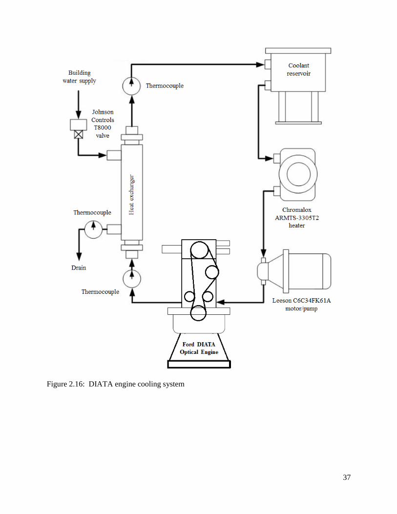
2.4.1 Starting & Motoring

Engine starting and motoring was performed by an air cooled General Electric DC Model

TLC-7.5 dynamometer, capable of providing 10 hp and absorbing 15 hp. The engine and

dynamometer were mounted to a steed bed plate, and connected by a drive shaft with a universal

joint on each end made by the Spicer Corporation.

21

A Dyne Systems DYNE-LOC IV dynamometer controller was used to operate the

dynamometer. The controller was located in the engine control room, and it provided a readout

of engine speed, torque, and power. It operated the engine at either a set rotational speed or at a

set torque. The engine torque was measured using an Omega LCCA-100 S-beam load cell at a

known distance from the axis of the dynamometer, and power was calculated based on speed and

torque. When motoring the engine, it is recommended to first bring the engine to 800 rpm and

let the speed and torque stabilize, then bring the engine to the desired speed. A detailed

schematic of the starting and motoring system can be found in Figure 2.18.

2.4.2 Fuel Injection & Spark

A master LabView program was used to control and monitor many aspects of the DIATA

engine data acquisition and controls system. Two main functions of this program were to supply

the signals that controlled the timing of fuel injection and spark. To properly time the injection

and spark, a BEI Motion Systems H25D shaft encoder provided crank angle information to

LabView.

The fuel injector was actuated using an in-house injector driver that used two voltage

doubling circuits to amplify a 12V source to 48V. A 5V TTL signal acted as a switch to drain

the voltage and actuate the injector solenoid. The injection duration was determined by the

duration of the TTL pulse, which was created using a Stanford Research Systems DG535 four

channel delay and pulse generator. A trigger signal sent by LabView determined the timing of

the first injection. If two injections were used, the Stanford box was used to set the delay time

between injections as well as the duration. In this situation, it was necessary to convert crank

angle degrees into time (dependent upon engine speed) to match the delay between pulses to the

desired number of degrees between injections.

22

The spark plug was fired using the circuitry described in Section 2.2.2. To actuate the

circuit, a 5V TTL pulse was generated in the master LabView program. The two important

parameters for controlling spark were dwell, or the time that the ignition coil charges, and the

spark timing. In a “points” style ignition system, dwell is determined by a cam lobe that closes

the circuit for a specified number of degrees. When the circuit was opened, the spark

discharged. Our system emulated this by sending the TTL signal with the duration equal to the

dwell time. The time was specified in LabView as a number of “ticks”, where a tick is defined

by the internal clock of the program and is equal to ¼ of a crank angle degree. The timing was

controlled such that the 5V TTL pulse ends at the desired spark discharge timing.

When running the DIATA engine, a “skip-fire” combustion pattern was used. The

engine combusted for three consecutive cycles, then motored for ten flushing cycles without

combustion. This reduced thermal loading on the optical components of the engine. During data

acquisition, the third combustion cycle was used for gathering pressure traces and imaging. This

allowed the engine to come to a quasi-steady state that yielded pressure traces and IMEP values

similar to continuous firing. It was found that firing only once followed by flushing cycles

generated much lower in-cylinder pressure and IMEP.

2.5 Data Acquisition

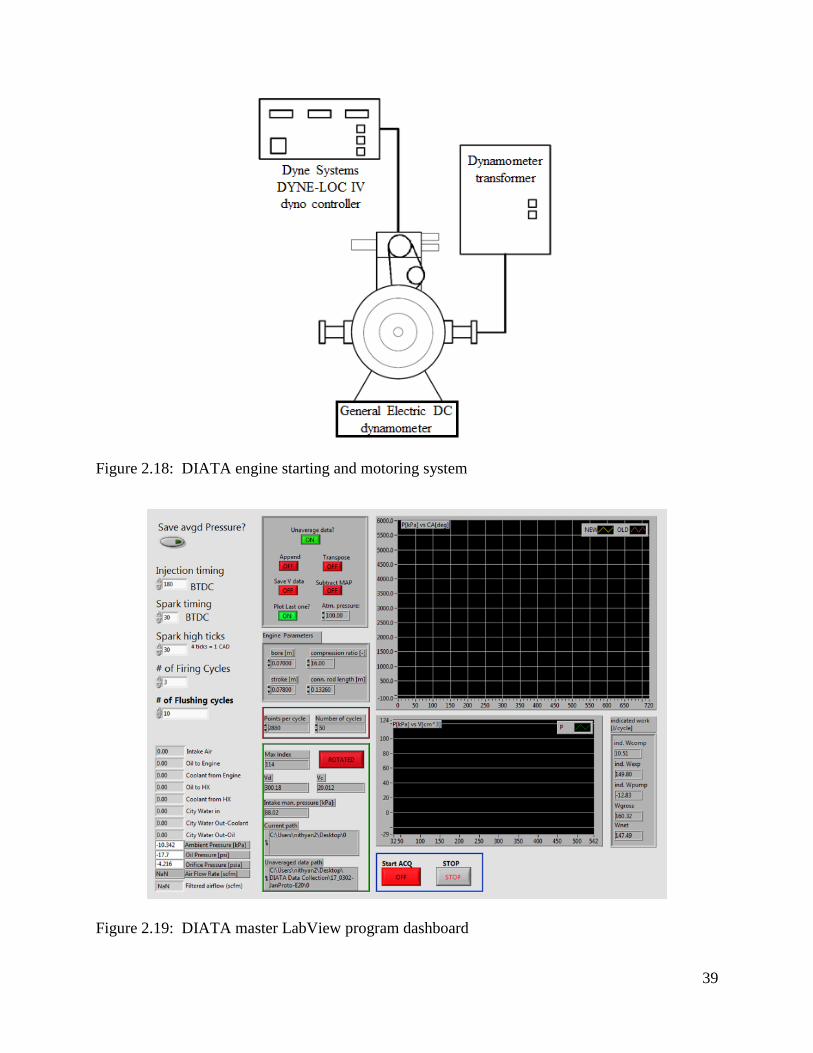
2.5.1 Engine Monitoring

The master LabView program that controlled fuel injection and spark was also

responsible for all engine monitoring in conjunction with several thermocouples and pressure

transducers. The program had a graphical user interface that acted as a dashboard for the engine,

shown in Figure 2.19. Ten thermocouples were used to monitor heat exchanger water

temperature, oil temperature, coolant temperature, and intake air temperature in several

23

locations. Several pressures were also measured including intake pressure, orifice pressure, and

oil pressure. In addition, intake mass air flow was calculated and displayed as described in

Section 2.3.2. Finally, a Kistler 6061B pressure transducer measured the in-cylinder pressure.

The transducer produced a small voltage signal that was amplified using a Kistler 5010 charge

amplifier. The amplifier sensitivity was set to 0.258 pC/MU and the scale was set to 2000

MU/Volt.

LabView recorded and saved the pressure traces for a specified number of cycles, then an

averaged pressure trace was displayed on the dashboard. When the engine was run in skip-fire

mode, an average of all pressure traces was not useful, as it would have included the flushing

(motoring) traces in the average pressure trace. A separate code was written using Excel VBA in

which each third combustion pressure trace could be averaged. Figure 2.20 shows the motoring

and combusting pressure traces for a particular run of data. The red pressure trace is the average

pressure of all of the combusting cycles. This code also plotted heat release rate and calculated

indicated mean effective pressure (IMEP), coefficient of variance (COV) of IMEP, and COV of

peak pressure.

2.5.2 Exhaust Gas Analysis

The engine exhaust gases were analyzed to study engine emissions, including unburned

hydrocarbons (UHC), carbon monoxide (CO), carbon dioxide (CO2), nitrogen oxides (NOx), and

soot. A Horiba MEXA-720 non-sampling type meter was used to measure NOx, as well as

equivalence ratio (λ) and percent O2 in the exhaust. A sensor was placed in the exhaust manifold

and the readings were transferred to the analyzer by a specialized cable. The measurement range

for NOx spanned from 0 to 3000 ppm by volume, with accuracies of ±30 ppm for 0-1000 ppm,

24

±3% for 1000-2000 ppm, and ±5% for 2000-3000 ppm. The analyzer averaged readings over a

60 second period to ensure reliable data collection.

UHC, CO, and CO2 were measured using a Horiba MEXA-554JU sampling type meter.

A fitting was added to the exhaust manifold from which a sampling tube was attached to carry a

continuous exhaust gas sample to the analyzer. This analyzer was a “dry” analyzer, meaning that

it was necessary for all water to be removed from the sample before analysis. To accomplish

this, the sampling tube was passed through an ice bath to condense the water from the exhaust

sample, and a trap in the line collected the liquid water. This exhaust analyzer had a

measurement range of 0-10,000 ppm for UHC, 0-20% by volume for CO2, and 0-10% by volume

for CO. Since the engine was skip-fired in a pattern of three firing cycles followed by 10

flushing cycles, UHC, CO, CO2, and NOx values were corrected by multiplying by a factor of

13/3.

Soot measurements were taken from the exhaust using a filter paper method. Raw

exhaust samples were drawn from the exhaust manifold through a fitting using a JB Industries

DV-142N 0.5 hp, 5 CFM vacuum pump. 7/8" round filter paper disks were cut from strips of

Grainger Industrial Supply 6T167 filter paper and placed into a collection housing taken from a

Bacharach True-Spot smoke meter. Exhaust gas was drawn through the filter paper for a

duration of 90 seconds while a flow meter monitored sampling flow rate. After being collected,

the blackening of the filter paper was recorded using a digital scanner, and filter smoke number

(FSN) was obtained using the method outlined in reference [11]. To correct FSN for skip-firing

conditions, the collection time was reduced by a factor of 3/13.

25

2.5.3 Imaging

In the optical engine, two types of in-cylinder imaging techniques were used: Mie

scattering and natural flame luminosity imaging. To study liquid spray penetration, images were

taken using Mie scattering. Mie scattering is a technique in which liquid fuel spray can be

visualized to provide qualitative information on spray evolution, transient liquid-phase

distribution, liquid penetration length, and spray interactions with the cylinder wall and piston

bowl. To perform Mie scattering, a light source must be directed into the combustion chamber

and the liquid fuel droplets scatter the light causing them to be visible to the camera. In this

study, an Oxford Lasers copper vapor laser (532 nm) was used as the light source, and a Vision

Research Phantom V7.0 high speed video camera was used to capture the images.

For Mie scattering, two different camera and laser configurations were used in

conjunction with several mirrors. The first configuration, 3-dimensional Mie scattering, allowed

the spray to be viewed from both the bottom of the piston and through the side window

simultaneously. In this configuration, the laser entered through the side window at a 15-degree

angle, and three 45-degree mirrors were placed such that one camera could capture both the

bottom and side view. The mirror below the piston was a UV enhanced aluminum coated

elliptical mirror with at 1.5" minor diameter (Edmund Optics #43-577) to fit inside the Bowditch

extension. The two mirrors used for the side view were 2" square protected aluminum mirrors

(Thor Labs ME2S-G01). The mirrors were chosen for their reflectance at 532 nm. It was

necessary to precisely adjust the direction of the incident laser light such that the spray was

visible through the bottom view, while the side view image was not saturated. The images were

taken at a resolution of 288 x 560. A schematic of the 3-dimensional Mie scattering setup is

26

shown in Figure 2.21. Figure 2.21 through Figure 2.23 are adapted from the Ph.D. thesis of

Tiegang Fang [12].

The second spray imaging configuration, 2-dimensional Mie scattering, took just side

view imaging through the side window. The camera was placed directly in line with the side

window, and the laser was directed through the bottom of the piston by way of the 45-degree

mirror. While 2-dimensional scattering does not provide a bottom view of the spray, it does have

a few distinct advantages over 3-dimensional Mie scattering. The first is that a higher resolution

image can be used for the side view, with a size of 464 x 336. There is a tradeoff between image

resolution and frame rate, so to increase image area to capture both views in the 3-dimensional

configuration while maintaining the same frame rate, the resolution must be decreased. The

second advantage is that illumination from below through the quartz piston provides a more even

illumination, and less glare on the piston and back cylinder wall. A schematic of the 2-

dimensional Mie scattering setup is shown in Figure 2.22.

For all spray imaging, the camera was set to record 12,000 frames per second, and the

camera was synced with the copper vapor laser. The camera exposure time was set to 1 μs, and

the laser provided one 25 ns pulse during each exposure. The camera aperture size (f-number)

was adjusted such that the spray was seen as brightly as possible without image saturation.

To study the combustion characteristics in the chamber, natural flame luminosity imaging

was used. In this technique, the natural luminosity of the combustion can be observed directly

using the camera, so no laser is needed. The imaging setup is nearly identical to the 3-

dimensional Mie scattering setup, except without the laser, and can be seen in Figure 2.23. The

camera was set to record 12,000 frames per second at a resolution of 288 x 560. All combustion

cases were taken at an exposure of 10 μs for comparison purposes, and some dimmer cases were

27

repeated at 30 μs for further investigation. For all combustion cases, the f-number was set to

f/4.5. The Phantom Vision software package that was provided with the camera was used to set

imaging parameters and view the raw image files.

28

2.6 Tables & Figures

Table 2.1: Specifications of the single-cylinder DIATA research engine

Displacement 300 cc

Compression ratio 16:1

Bore 70 mm

Stroke 78 mm

Number of valves 4 (2 intake, 2 exhaust)

Swirl ratio 2.5 (low); 4.0 (high)

Intake valve diameter 24 mm

Exhaust valve diameter 21 mm

Maximum valve lift 7.30 / 7.67 mm (Intake / Exhaust)

Valve timing (1 mm lift): IVO 13° ATDC

IVC 20° ABDC

EVO 33° BBDC

EVC 18° BTDC

Figure 2.1: 45-degree mirror seen mounted inside Bowditch extension (cylinder head and liner

removed)

29

Figure 2.2: Optical window and window blank

Figure 2.3: Schematic of optical section of DIATA engine

30

Figure 2.4: Picture of the DIATA optical engine

Figure 2.5: (a) NGK ER9HE spark plug before (right) and after (left) modification, (b) spark

plug tool mating with spark plug

31

Figure 2.6: Spark plug hole location in cylinder head CAD model

Figure 2.7: Cylinder head mounted in 3-axis mill for spark plug hole machining

32

Figure 2.8: Spark plug installed in cylinder head

Figure 2.9: Ignition circuit, first iteration

+12 VIgnition

Coil

VB921

ZVFI

5V TTL Pulse

From LabView

332 Ω

33

Figure 2.10: Ignition circuit, second iteration using MSD 6A spark booster

Figure 2.11: Ignition circuit, final iteration using Dynatek DBR-1 spark booster

+12 V

Ignition

Coil

VB921

ZVFI

5V TTL Pulse

From LabView

MSD 6A

Ign. Booster

332 Ω

+12 VIgnition

Coil

VB921

ZVFI

5V TTL Pulse

From LabView

Dynatek

DBR-1 Booster

332 Ω

34

Figure 2.12: Clearance volume calculation zones

Figure 2.13: Fuel injector and mounting sleeve assembly

35

Figure 2.14: DIATA engine fuel supply system

36

Figure 2.15: DIATA engine air supply system

37

Figure 2.16: DIATA engine cooling system

38

Figure 2.17: DIATA engine lubrication system

39

Figure 2.18: DIATA engine starting and motoring system

Figure 2.19: DIATA master LabView program dashboard

40

Figure 2.20: IMEP calculator Excel program, average pressure trace of combusting cycles

shown in red

Figure 2.21: 3-dimensional Mie scattering imaging setup

41

Figure 2.22: 2-dimensional Mie scattering imaging setup

Figure 2.23: 3-dimensional natural flame luminosity imaging setup

42

Chapter 3: Experimental Procedure

3.1 Equipment Calibration

3.1.1 Injection Mass Calibration

The injected mass of each injection of the fuel injector was controlled by the injection

pulse duration. To accurately control injected mass, the injected mass versus injection duration

was calibrated. To calibrate injection mass, the injector was set up outside of the engine, and the

fuel was pressurized. A collection bottle was placed over the injector nozzle, and fuel was

injected for 300 injection cycles at a specified injection duration. The collection bottle was

weighed before and after to a precision of .01 gram. The total mass was divided by 300 cycles to

obtain the mass per injection. This process was repeated for injection durations from the

minimum duration the injector would inject (0.2 ms) up to the maximum desired injection

duration of 1.8 ms in increments of 0.2 ms. A calibration curve was fit to these data points with

an R2 value of 0.9999. The calibration curve was then used to obtain the pulse duration for any

desired injection mass.

3.1.2 Pressure Transducer Calibration

Several pressure transducers were used in the DIATA optical engine experiments. The

transducers have a voltage output that is read by the LabView program. Over time the output

voltage can change, so the pressure transducers are calibrated yearly. To calibrate the

transducer, the transducer was attached to a calibration unit with pressurized gas and a precise

analog pressure gauge. The pressure was adjusted to several points over the operating range of

the pressure transducer, and the voltage was recorded. A linear fit was then assigned to correlate

voltage to pressure, and was input into the LabView code. This calibration is particularly

43

important for the transducers used to measure air flow rate, as the mass flow rate of air

determines the stoichiometric fuel mass.

3.2 Metal Engine Operation

3.2.1 Data Collection

The optical engine with all optical components removed and the metal piston and side

window blanks installed is referred to as the metal engine. The metal engine was used prior to

any optical study to assess the performance and emissions of each operating condition, as well as

to study the combustion stability, measured by COV IMEP and COV peak pressure. Any

conditions deemed too unstable (COVs greater than 10%) were not studied in the optical

configuration, and all conditions run in the optical engine were first tested on the metal engine.

When running the metal engine, all procedures used in the optical engine were followed

to ensure consistency of results between the two. First, the coolant and engine oil were

preheated, and when combusting, the same skip firing pattern was used. To operate the engine,

first they dynamometer was turned on to 800 rpm and allowed to stabilize. Then, the

dynamometer was brought to operating speed and allowed to stabilize. Once the engine was

stable at the desired operating speed, the power supply to the fuel injector was turned on. The

spark plug begins arcing as soon as the engine starts to rotate, so the fuel injector power switch

determined when the engine was combusting or motoring.

Once the engine was firing, it was allowed to run for one minute to reach steady state

before gathering data. After one minute, the soot collection vacuum pump was turned on, and a

ball valve between the exhaust manifold and the soot collection line was opened. Pressure traces

from 200 cycles were collected and saved. After 90 seconds, the soot collection valve was

closed and the vacuum pump turned off. NOx values were recorded from the Horiba MEXA-

44

720 analyzer, and UHC, CO, CO2, and O2 values were recorded from the Horiba MEXA-554JU

analyzer. Once the data was recorded, the fuel injector and dynamometer were turned off. The

soot sample was placed into a labeled compartment in a clean plastic sample box with dividers.

The engine was allowed to rest ten minutes between each run to return to the baseline operating

temperature, then the process was repeated for the next operating condition.

3.2.2 Data Processing

After 200 pressure cycles were recorded, the data was saved in a .txt file. That file was

imported into an Excel IMEP calculator program that was developed in-house, and each

individual trace was displayed. From the pressure data, the IMEP was calculated. The average

of the combustion pressure traces was then smoothed using a seven-point running average, and

from that the heat release rate was calculated and plotted. The program also plotted mass

fraction burned and calculated CA10, CA50, and CA90, the crank angles at which 10, 50 and 90

percent of the heat has been released, respectively. The ignition delay and combustion duration

were then calculated. In this study, ignition delay is defined as the crank angle degrees between

spark timing and CA10, and combustion duration is defined as the crank angle degrees between

CA10 and CA90. The emissions data were then corrected for the skip-firing conditions and the

soot samples were processed using the procedures described in Section 2.5.2.

3.3 Optical Engine Operation

3.3.1 Spray Imaging

To conduct spray imaging, the optics were first set up in the 2- or 3-dimensional

configuration, then the laser was turned on and adjusted for proper illumination. To begin

imaging, the engine was first brought to operating speed. Once engine speed stabilized, power to

the fuel injector was turned on. Injecting cycles used the same 3 fire, 10 flush skip-fire pattern as

45

combusting cycles, except the spark plug was disconnected so no combustion occurred.

Immediately after the injector was turned on the camera was activated, and the first fuel injection

provided the trigger to capture images. The subsequent two injecting cycles were fully captured

by the camera. It was important to synchronize turning on the injector with activating the

camera such that the first set of three injections were captured. If too many injection cycles

occur before the camera begins capturing images, a fuel film will form on the optical side

window and obstruct the images. Once the camera captured a set of injecting cycles, injector

power was turned off, and the dynamometer was shut down. Then, the images were viewed in

the Phantom Vision software, and the desired frames were selected and saved as .cine files.

After the images were saved, the process was repeated for the next operating condition.

3.3.2 Combustion Imaging

To conduct combustion imaging, the procedure was similar to spray imaging. Once the

camera and optics were set up, the engine was brought to operating speed. Once engine speed

had stabilized, the power to the injector was turned on. In this case, the spark plug was

connected, so as soon as the injector was turned on, combustion began to occur. The same skip-

firing mode was used. For the combustion imaging, rather than capturing images on the first set

of injecting cycles, the engine was allowed to run for ten sets of 3 fire-10 flush to allow

conditions to reach a quasi-steady state. After ten 3 fire-10 flush sets, the camera was activated

and the first injection triggered the camera to capture images. The camera fully captured the

subsequent two combusting cycles. Also, a set of three combustion pressure traces were

recorded corresponding to the imaged cycles. Once the camera captured a set of combusting

cycles, injector power was turned off, and the dynamometer was shut down. The frames from

the third combusting cycle were saved as a .cine file. The engine was allowed five minutes

46

between each run to return to the baseline operating temperature, then the process was repeated

for the next operating condition.

3.3.3 Image Processing

For spray and combustion imaging, the raw .cine files were processed using separate

Matlab programs that were developed in-house. For the spray imaging, the program took each

frame and stamped the crank angle (ATDC) as well as any other pertinent information including

injector and fuel used. A black mask was laid over each image such than only the views through

the side window and piston were visible, and the surrounding metal was covered. The program

also created an .avi video file of each injection. Images from each case were selected at even

crank angle increments to show the important features of the spray and laid out into figures.

For 2-dimensional Mie scattering, a background subtraction technique was employed. A

set of images was taken using the same optics configuration and camera settings, the only

difference being that no fuel was injected. The intensity of these pixels was subtracted from the

spray image pixels, eliminating most of the glare from the laser and making the background

completely black.

For natural flame luminosity imaging, a similar Matlab program was used. In addition to

the above steps, the images were overlaid with a color map to create the orange coloring from the

black and white image. For each frame, the spatially integrated natural luminosity (SINL) was

calculated by integrating the pixel intensity over the bottom view image from each frame, and

SINL was plotted with respect to crank angle. To quantify the natural luminosity of the entire

combustion cycle, the time integrated natural luminosity (TINL) was calculated by integrating

the SINL curve over time. In addition, for each imaging condition, the pressure traces recorded

were processed in the same way as the metal engine data.

47

Chapter 4: Results & Discussion

4.1 Metal Engine Results

Using the metal engine configuration, general combustion characteristics of the DIATA

engine were observed. As this engine had never been operated in the GDI mode using the new

injector and piston geometry, a broad range of operating conditions were tested to learn the basic

functionality of the new setup. Due to the high compression ratio, the baseline fuel used was a

blend of 80 percent 90-octane pure gasoline and 20 percent ethanol, referred to as E20. The fuel

injector used was the commercially available Delphi GDI fuel injector. A load sweep was

performed at stoichiometric conditions by adjusting intake pressure from 10 to 12 psi. A lean

equivalence ratio sweep was performed from stoichiometric down to Φ = 0.6 at an intake

pressure of 11 psi. In addition, at stoichiometric conditions and 11 psi intake pressure, an

injection split sweep, a first injection timing sweep, and a second injection timing sweep were

performed. For each of these sweeps, emissions (NOx, soot, CO, UHC), performance (IMEP,

indicated efficiency), stability (COV IMEP, COV peak pressure), and combustion characteristics

(ignition delay, CA50, combustion duration) were recorded.

4.1.1 Load Sweep

Figure 4.1 shows in-cylinder pressure and heat release rate for a 180° BTDC single

injection load sweep. Load was adjusted by adjusting intake pressure, while maintaining

stoichiometric conditions. With a single injection at 180° BTDC, the mixture was mostly

premixed by the start of combustion. From Figure 4.2 it was observed that as load decreased,

NOx and soot both decreased. NOx formation is highly dependent on temperature, and at higher

load, in-cylinder pressure was much higher, leading to higher temperatures and thus more NOx

formation. Since the overall mass of fuel and air decreases with lower load, and stoichiometric

48

premixed conditions were maintained, soot mass that was produced, and thus FSN, decreased

proportionally. Unburned hydrocarbons remained essentially the same, and CO emissions were

lowest at 10 psi intake pressure.

From Figure 4.3 it was observed IMEP decreased with decreasing load. This makes

sense as IMEP is often used as a measure of load, and is defined as the average pressure acting

on the piston through the combustion cycle. The indicated efficiency, on the other hand, was

highest at lowest load, meaning that decrease in IMEP was outweighed by the decrease in

injected fuel mass. In terms of stability, it was observed that 11 psi had the lowest COV IMEP,

and 10 psi had the lowest COV peak pressure, showing that lower load cases were more stable.

With respect to combustion phasing, changing load had a distinct effect. Figure 4.4 shows

that the ignition delay, that is the duration between spark and CA10, increased as load decreased.

This was likely due to lower temperature and pressure at lower load causing the mixture to be

slightly volatile. The CA50 values show that combustion phasing was also retarded at lower

load.

4.1.2 Injection Split Sweep

An injection split sweep was performed at stoichiometric conditions at 11 psi intake

pressure. For this sweep, the first injection was fixed at 180° BTDC and the second injection

was fixed at 35° BTDC. The sweep consisted of a single injection; a double injection with 90

percent of the fuel injected during the first injection, referred to as a 90/10 split; and a double

injection 80/20 split. Figure 4.5 shows the in-cylinder pressure and heat release rate for the three

conditions. From Figure 4.6 it was observed that the NOx and CO emissions were much lower

in the 90/10 split condition. In addition, the 90/10 spilt held a slight advantage for soot

49

emissions. The lowest UHC emissions were seen in the single injection case, since this case was

more premixed than the stratified double injection cases.

COV IMEP and COV peak pressure values in Figure 4.7 show that the stability is also

best using a 90/10 split. The penalty for using a 90/10 split over single injection was a 9% UHC

increase, however the 90/10 split consistently gave a 20% improvement in COV values. Due to

the lowered emissions and increased stability, a 90/10 split was chosen for all further double

injection cases. Figure 4.8 shows that phasing differences are very small between the three

cases.

4.1.3 Equivalence Ratio Sweep

Figure 4.9 shows the in-cylinder pressure and heat release rate for a double injection

equivalence ratio sweep from 1.0 to 0.6. Below an equivalence ratio of 0.6, the engine did not

fire. The first injection was at 180° BTDC and the second injection was at 35° BTDC.

Figure 4.10 shows emissions data for the equivalence ratio sweep. It can be seen that

NOx first increases as the mixture is leaned, then drops off starting at an equivalence ratio of 0.7.

The two main factors that influence NOx production are temperature, as well as the presence of

excess nitrogen and oxygen. Increasing NOx as the mixture became leaner from stoichiometric

was due to a greater excess of air, allowing more nitrogen and oxygen to form NOx. After an

equivalence ratio of 0.8, the NOx dropped off due to lower temperatures in the cylinder. Soot

decreased as the mixture became leaner. Soot formation occurs when rich pockets of fuel

undergo pyrolysis in the absence of oxygen, so with a leaner mixture, lower soot emissions are

expected. UHC emissions remained constant, except for at the leanest case they increased,

indicating less complete combustion at an equivalence ratio of 0.6 because the mixture was

approaching the flammability limit. CO emissions decreased as the mixture became leaner,

50

which is expected because an increased excess of oxygen helps CO oxidize completely to form

CO2.

Figure 4.11 shows that as the mixture was leaned, IMEP decreased. At first, the decrease

in IMEP was relatively small, and indicated efficiency increased due to less fuel input. There

was a drop in efficiency at the = 0.6 case due to the mixture being too lean to burn well, which

was also seen in the UHC trend. There was not a distinct trend with respect to stability, however

both COV IMEP and COV peak pressure showed that the stoichiometric case was the most

stable.

Figure 4.12 shows that as the mixture was leaned, combustion phasing became more

retarded. Ignition delay also increased as the mixture became leaner. No clear trend was

observed in the combustion duration except that the stoichiometric case had a distinctly shorter

combustion duration.

4.1.4 Injection Timing Sweeps

In addition to load, injection split, and equivalence ratio, injection timing was also

studied. A sweep of first injection timing was conducted with the second injection timing held

constant, and a sweep of second injection timing was conducted with the first injection timing

held constant. For the first injection timing sweep, the timing was swept from 200° BTDC to

160° BTDC, with second injection timing held at 35° BTDC. The range of the sweep was

chosen based on the range that the engine ran stably during preliminary testing.

Figure 4.13 shows the in-cylinder pressure and heat release rate for the first injection

timing sweep. Figure 4.14 shows emissions results for the sweep. It was observed that NOx and

UHC increased linearly as first injection timing was retarded. Soot and CO emissions, on the

other hand, decreased linearly with retarded timing. From Figure 4.15 it was observed that

51

IMEP increased with retarded first injection timing, however higher stability was seen in the

more advanced timings. Figure 4.16 shows that combustion phasing was retarded slightly as the

injection was retarded, but the effect of first injection timing on ignition delay and combustion

duration was very small.

Second injection timing was also swept. The first injection was held at 180° BTDC,

while the second injection was varied from 40° to 30° BTDC. Figure 4.17 shows the in-cylinder

pressure and heat release rate for the second injection timing sweep. From Figure 4.18 it can be

seen that NOx decreased with retarded second injection timing. Soot, on the other hand,

increased with retarded second injection timing. This is expected because retarding the injection

lowers the amount of time for the stratified charge to mix, leaving rich regions that cause soot

formation. Figure 4.19 shows that second injection timing had very little effect on engine

performance, likely due to the fact that the second injection consisted of only ten percent of the

energy input. Figure 4.20 shows that retarding the second injection timing very slightly retarded

combustion phasing, but ignition delay and combustion duration were affected very little.

4.2 Optical Engine Results

After metal engine testing was complete, the optical piston and an optical side window

were installed on the engine. Optical engine imaging was taken in two steps. First, Mie

scattering spray imaging was conducted for various operating conditions using the copper vapor

laser as illumination. Then, the laser was removed and natural flame luminosity combustion

imaging was conducted.

4.2.1 Spray Imaging

The effect of changing the double injection split was studied using Mie scattering spray

imaging. Side view images of first and second injections were taken for single injection, a 90/10

52

split, and an 80/20 split with a first injection timing of 180° BTDC and a second injection timing

of 35° BTDC. For the first injection, images are shown in Figure 4.21, displayed in in 2.4-

degree increments starting at 175.98° BTDC, and each image is stamped with the corresponding

crank angle. In the first three rows of images, the injection for all three cases looks the same.

Since fuel quantity was metered by injection duration, the difference between the cases is when

injection ends. The shortest first injection was the 80/20 split case, which had a duration of 10.3

degrees, stopping between the third and fourth row of images. The 90/10 case had a duration of

10.9 degrees and stopped just before the fourth image was captured. The single injection case

had a duration of 11.4 degrees, and was still injecting when the fourth row of images was

captured. Consequently, from the fourth row onward it can be seen that there is less fuel in the

chamber as the first injection is shortened.

The images show that the fuel was injected at a wide injection angle and the jets were

initially parallel to the cylinder head. Once the jets reached the wall, the fuel mist travelled

downward in an umbrella shape and some fuel was deposited on the cylinder walls. The smaller

the first injection, the less fuel travelled downward along the cylinder walls, which can be

observed in the last two rows of Figure 4.21.

Figure 4.22 shows the difference between the second injections from 90/10 and 80/20

splits. Even with adjusting laser and camera settings, the second injection in the 90/10 case was

very difficult to see. It was observed most clearly by viewing the images frame-by-frame in the

12,000 frame per second video, but even then, only several fuel droplets could be seen. For the

80/20 split, distinct jets can be seen. In the fourth and fifth row of images, it can be seen that the

jets began to impinge on the piston, creating a liquid fuel film.

53

A single injection timing sweep was also investigated using Mie scattering spray

imaging. Figure 4.23 shows a comparison of 2-dimensional background subtracted Mie

scattering images of injections at 220°, 180°, and 140° BTDC. Since the injections began at

different times, images from each case were aligned with respect to crank angle degrees after

start of injection (SOI). Due to the frame rate, it was not possible to perfectly align the images in

this respect, but they are aligned within 0.5 crank angle degrees after SOI. The images are

spaced in 2.4-degree increments.

In the DIATA engine, the intake valves close at 160° BTDC. In the earliest (220°

BTDC) injection case, it was observed that the intake valves were still fully open, and the wide

spray angle caused impingement on the valves. On the other hand, having the valves open

increased charge motion, and enhanced mixing. In the latest (140° BTDC) injection case, the

intake valves were fully closed, and it was observed that the spray was much more symmetrical.

However, charge motion during injection was lower due to the closed valves. The 180° BTDC

injection combined the best features of both of these injections. During the injection, intake

valves were closed partially, limiting valve impingement, yet charge motion was enhanced.

Figure 4.24 shows 3-dimensional Mie scattering images for the same comparison. Due to

the design of the piston extension, the 45-degree mirror is partially or fully blocked when the

piston is near bottom dead center. Because of this, the bottom view images for the 220° and

180° cases were not particularly useful. For the 140° case, the bottom view of the spray started

to become visible. 3-dimensional imaging was most useful after 120° BTDC where the bottom

view was fully visible.

54

4.2.2 Combustion Imaging

To study combustion, images were captured using 3-dimensional natural flame

luminosity imaging. Using single injection at 180° BTDC, a load sweep and an equivalence

ratio sweep were imaged. Images were captured in 6-degree increments, starting at 13.22°

BTDC. Figure 4.25 shows natural luminosity images for a single injection stoichiometric load

sweep at 12, 11, and 10 psi intake pressure. Because of a single early injection, the mixture is

mostly premixed. This can be observed from the images by the uniform luminosity during the

combustion duration. Figure 4.26 shows the SINL and TINL information from the images, and

can give further insights. Firstly, the phasing of the SINL curve is clearly retarded at lowest

load, which was also observed in the metal engine data. However, the SINL phasing for 11 and

12 psi was roughly the same. TINL data can be used as an indication of soot concentration over

the whole cycle [13]. The trend for TINL in Figure 4.26 shows that TINL increased with

increasing load, and the data matches the FSN data in Figure 4.2 almost identically.

Natural luminosity images were also taken for a single injection equivalence ratio sweep

from = 1 to = 0.7. Figure 4.27 shows 3-dimensional natural flame luminosity images for

each operating condition. The uniform luminosity from premixed combustion was also observed

in this sweep. Figure 4.28 shows SINL and TINL data for the equivalence ratio sweep. The

SINL curves show that combustion phasing was retarded as the mixture was leaned. This was

also seen in the metal engine data. While metal engine data was taken using double injection,

and the images were taken using single injection, the TINL and FSN trends also agree with

respect to equivalence ratio.

55

4.3 Tables & Figures

Figure 4.1: Single injection load sweep in-cylinder pressure and heat release rate

Figure 4.2: Single injection load sweep emissions

56

Figure 4.3: Single injection load sweep performance and stability

Figure 4.4: Single Injection load sweep combustion characteristics

57

Figure 4.5: Injection split sweep in-cylinder pressure and heat release rate

Figure 4.6: Injection split sweep emissions

58

Figure 4.7: Injection split sweep performance and stability

Figure 4.8: Injection split sweep combustion characteristics

59

Figure 4.9: Equivalence ratio sweep in-cylinder pressure and heat release rate

Figure 4.10: Equivalence ratio sweep emissions

60

Figure 4.11: Equivalence ratio sweep performance and stability

Figure 4.12: Equivalence ratio sweep combustion characteristics

61

Figure 4.13: First injection timing sweep in-cylinder pressure and heat release rate

Figure 4.14: First injection timing sweep emissions

62

Figure 4.15: First injection timing sweep performance and stability

Figure 4.16: First injection timing sweep combustion characteristics

63

Figure 4.17: Second injection timing sweep in-cylinder pressure and heat release rate

Figure 4.18: Second injection timing sweep emissions

64

Figure 4.19: Second injection timing sweep performance and stability

Figure 4.20: Second injection timing sweep combustion characteristics

65

Figure 4.21: Injection split sweep first injection 2-dimensional Mie scattering spray imaging

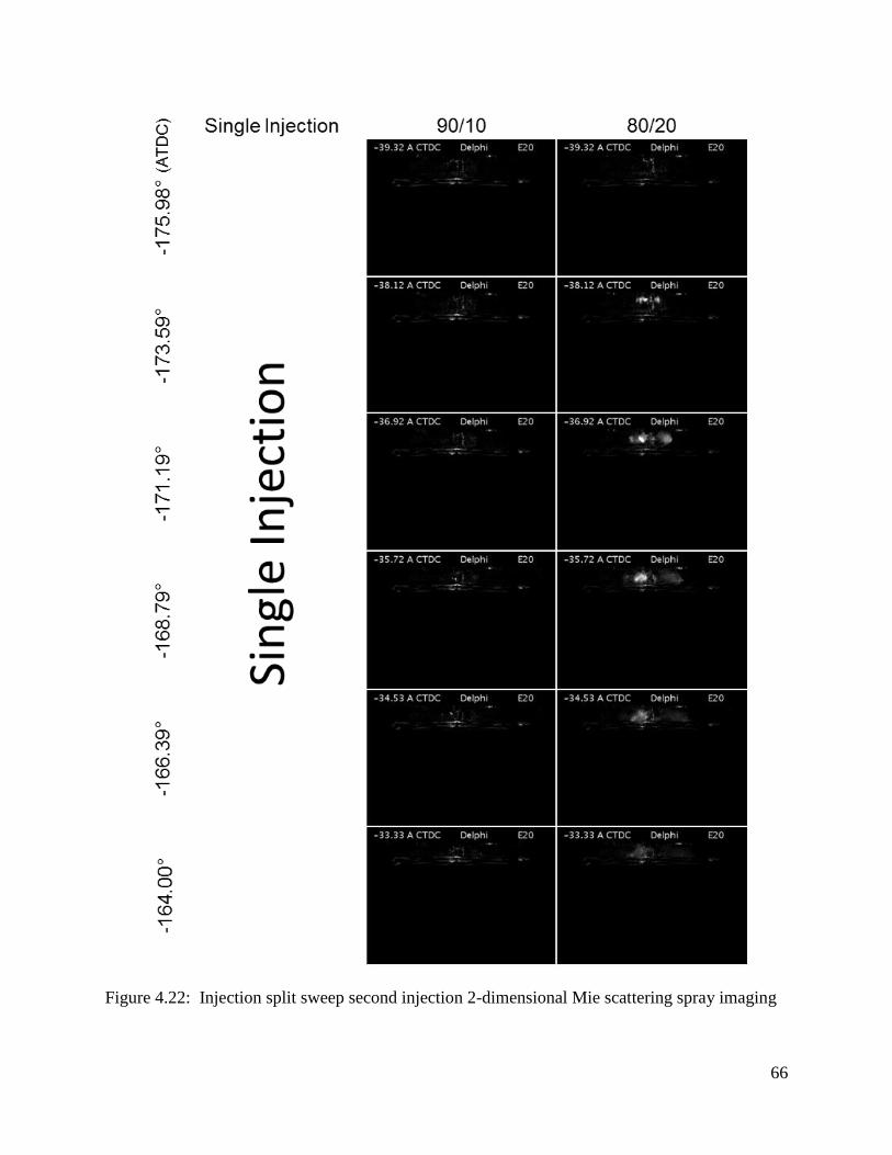
66

Figure 4.22: Injection split sweep second injection 2-dimensional Mie scattering spray imaging

67

Figure 4.23: Single injection timing sweep 2-dimensional Mie scattering spray imaging

68

Figure 4.24: Single injection timing sweep 3-dimensional Mie scattering spray imaging

69

Figure 4.25: Single injection load sweep 3-dimensional natural flame luminosity imaging

Figure 4.26: Single injection load sweep spatially and temporally integrated natural luminosity

70

Figure 4.27: Single injection equivalence ratio sweep 3-dimensional natural flame luminosity

imaging

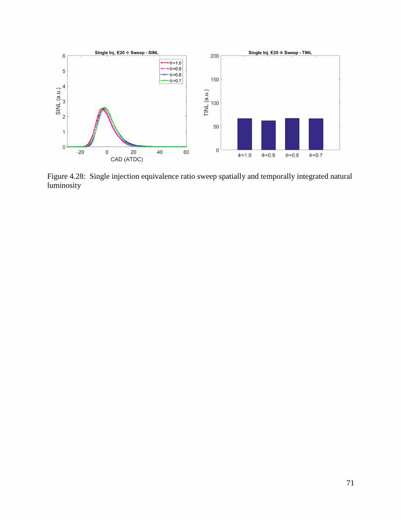
71

Figure 4.28: Single injection equivalence ratio sweep spatially and temporally integrated natural

luminosity

72

Chapter 5: Conclusions

In this study, a single-cylinder optically accessible engine was built to visualize gasoline

direct injection combustion. The engine was originally designed for compression ignition

combustion, but was modified to be fitted with a spark ignition system, as well as a new piston

geometry and fuel injector. When engine setup was complete, the study was broken into two

parts: metal engine testing and optical engine testing. In the metal engine configuration, the

optical components were swapped with metal replacements, and engine performance, stability,

and emissions were studied. In the optical configuration, Mie scattering and natural flame

luminosity imaging were used to study injector spray and combustion, respectively. Experiments

were run with a commercially available Delphi GDI fuel injector, using a 20 percent ethanol 80

percent pure gasoline blend as fuel. Conclusions from this study are as follows:

A single-cylinder, optically accessible research engine was converted from compression

ignition to gasoline direct injection.

A spark system was designed using a VB921 ignition coil driver in conjunction with

LabView and a Dynatek ignition booster box.

The cylinder head was modified to incorporate a custom spark plug and the piston and

compression ratio were changed for gasoline combustion.

A Phantom V7.0 high-speed camera was used to visualize fuel injector spray and

combustion characteristics within the combustion chamber.

Emissions and performance data were collected using a non-optical aluminum piston setup

to provide further information about the combustion.

73

It was found that a double injection with a 90 percent/10 percent first/second injection split

provided the lowest NOx, CO, and soot emissions, as well has lowest coefficient of

variation for IMEP and peak in-cylinder pressure.

It was found that a first injection timing of 180° BTDC was best for fuel mixing because

earlier injections impinge on the intake valves and later injections lack the charge motion

due to the intake valves being fully closed.

74

References

[1] Light Duty Vehicle Stock by Technology Type, Annual Energy Outlook, United States

Energy Information Administration, 2017.

[2] Average Fuel Efficiency of U.S. Light Duty Vehicles, National Transportation Statistics,

Bureau of Transportation Statistics, United States Department of Transportation, 2016.

[3] Draft Technical Assessment Report: Midterm Evaluation of Light-Duty Vehicle

Greenhouse Gas Emission Standards and Corporate Average Fuel Economy Standards for

Model Years 2022-2025, Office of Transportation and Air Quality, United States

Environmental Protection Agency, 2016.

[4] Guo, H., Ma, X., Li, Y., Liang, S., Wang, Z., Xu, H. and Wang, J., 2017. Effect of flash

boiling on microscopic and macroscopic spray characteristics in optical GDI engine.

Fuel, 190, pp.79-89.

[5] Song, J. and Park, S., 2015. Effect of injection strategy on the spray development process

in a single-cylinder optical GDI engine. Atomization and Sprays, 25(9).

[6] Catapano, F., Di Iorio, S., Lazzaro, M., Sementa, P. and Vaglieco, B.M., 2013.

Characterization of ethanol blends combustion processes and soot formation in a GDI

optical engine (No. 2013-01-1316). SAE Technical Paper.

[7] Catapano, F., Sementa, P. and Vaglieco, B.M., 2016. Air-fuel mixing and combustion

behavior of gasoline-ethanol blends in a GDI wall-guided turbocharged multi-cylinder

optical engine. Renewable Energy, 96, pp.319-332.

[8] Dahlander, P. and Hemdal, S., 2015. High-speed photography of stratified combustion in

an optical GDI engine for different triple injection strategies (No. 2015-01-0745). SAE

Technical Paper.

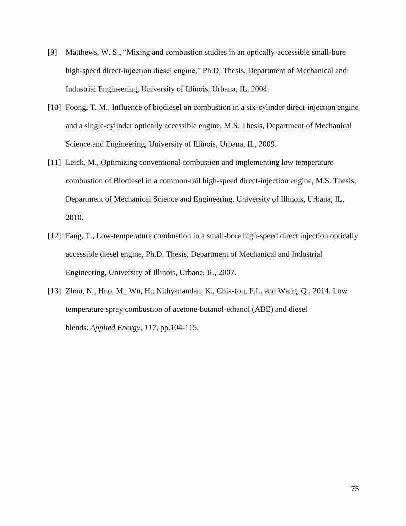
75

[9] Matthews, W. S., “Mixing and combustion studies in an optically-accessible small-bore

high-speed direct-injection diesel engine,” Ph.D. Thesis, Department of Mechanical and

Industrial Engineering, University of Illinois, Urbana, IL, 2004.

[10] Foong, T. M., Influence of biodiesel on combustion in a six-cylinder direct-injection engine

and a single-cylinder optically accessible engine, M.S. Thesis, Department of Mechanical

Science and Engineering, University of Illinois, Urbana, IL, 2009.

[11] Leick, M., Optimizing conventional combustion and implementing low temperature

combustion of Biodiesel in a common-rail high-speed direct-injection engine, M.S. Thesis,

Department of Mechanical Science and Engineering, University of Illinois, Urbana, IL,

2010.

[12] Fang, T., Low-temperature combustion in a small-bore high-speed direct injection optically

accessible diesel engine, Ph.D. Thesis, Department of Mechanical and Industrial

Engineering, University of Illinois, Urbana, IL, 2007.

[13] Zhou, N., Huo, M., Wu, H., Nithyanandan, K., Chia-fon, F.L. and Wang, Q., 2014. Low

temperature spray combustion of acetone-butanol-ethanol (ABE) and diesel

blends. Applied Energy, 117, pp.104-115.

76

Appendix A: Troubleshooting

Several common issues were faced when running the DIATA engine. Suggested

solutions are provided below.

Issue 1: The engine is not firing.

Check:

Is the injector injecting? (See Issue 2)

Is the spark plug arcing? (See Issue 4)

Issue 2: The injector is not injecting.

Check:

Is there fuel in the tank?

Is the fuel tank pressurized?

Is the injector actuating (clicking)? (See Issue 3)

Issue 3: Injector is not actuating (clicking).

Check:

Is the 12 V supply on?

Is the pulse generator turned on?

Is the fuse in the injector driver box good?

Is the LabView output set to the correct channel?

Issue 4: Spark plug not arcing.

Check:

Is the spark plug switch turned on?

Is the battery voltage high enough? (Should be greater than 12 V)

Are the spark “ticks” set to a high enough value?

77

Does the spark plug boot have any holes in it?

Is the LabView output set to the correct channel?

Issue 5: The dyno is not turning on.

Check:

Are the 20A fuses blown?

78

Appendix B: Engine Startup Checklist

Before turning on the dyno, there is a short list of important safety items that must be

checked every time the engine is run. They are listed below.

1. Is the nitrogen for the cylinder liner hydraulic system is pressurized?

2. Are both oil pumps are turned on?

3. Is the coolant pump is turned on?

4. Is the air supply is turned on and set to the desired intake pressure?

5. Is at least one intake runner ball valve is open.

If the answer to any of these questions is not yes, a major engine failure is likely.