Embed Size (px)
Citation preview

Alex De Deken
methods and DEM simulations
Design of rockfall protection metallic fences using similarity
Academic year 2015-2016
Faculty of Engineering and Architecture
Chair: Prof. dr. ir. Luc Taerwe
Department of Structural Engineering
Master of Science in de industriële wetenschappen: bouwkunde
Master's dissertation submitted in order to obtain the academic degree of
Supervisors: Prof. Patrick Ampe, Anthony Tetaert
Design of rockfall metallic fences
using similarity methods and
DEM simulations.
Master Thesis
A. De Deken
Supervisors of the Master Thesis : D. Bertrand (INSA Lyon) - I.
Olmedo and P. Robit (GTS)
June 25, 2016

This master dissertation contains confidential information and confiden-tial research results proprietary to INSA Lyon. It is strictly forbidden topublish, cite or make public in any way this master dissertation or any partthereof without the express written permission of INSA Lyon. Under no cir-cumstance this master dissertation may be communicated to or put at thedisposal of third parties. Photocopying or duplicating it in any other wayis strictly prohibited. Disregarding the confidential nature of this masterdissertation may cause irremediable damage to INSA Lyon.
1

Design of rockfall metallic fences
using similarity methods and
DEM simulations.
Master Thesis
A. De Deken
Supervisors of the Master Thesis : D. Bertrand (INSA Lyon) - I.
Olmedo and P. Robit (GTS)
June 25, 2016

Abstract
Due today’s expansion of infrastructure and housing in mountain-ous environments, they become more vulnerable to several naturalhazards such as rockfall. Placing of flexible metal nets provides a so-lution for protecting these areas. Testing needs to be done to optimisethe use of the flexible structures. The costs of these experiments arevery high, wherefore simulations offers a solution to this problem. Thispaper proposes an analysis for the development of scaling laws to ex-plore the potential behaviour of prototype structures used for rockfallprotection systems. Dimensional analysis will be the tool to achievesimilarity between the model and the prototype, mainly using dimen-sionless parameters. Experimental data will be provided by numericalmodulations, constructed with PFC and Matlab, to verify the scalinglaws. Dimensional analysis will first be performed on a simple system(cable), afterwards on more complex structures (stitch/mesh).

Acknowledgements
This master thesis gave me the chance to broaden my knowledgein the area of dimensional analysis. More specifically, the theoreti-cal and practical application of dimensional analysis on simple, andlater on, more complex structures. During this research I’ve receivedexcellent guidance from prof. D. Bertrand at INSA Lyon, who wasavailable every day to help me with certain problems that I occasion-ally came across. I also want to express my sincere gratitude to thepeople of GTS, more specifically I. Olmedo and P. Robit, for givinghelpful feedback and time to assist me in this research. I am grateful tothe University of Ghent for giving me the opportunity to do my masterthesis abroad and offering all necessary help with my application atINSA.

Contents
1 State of the art 91.1 Rockfall and mitigation systems . . . . . . . . . . . . . . . . . 9
1.1.1 Mitigation procedures: . . . . . . . . . . . . . . . . . . 91.1.2 Protection Systems: . . . . . . . . . . . . . . . . . . . . 10
1.1.2.1 Flexible Protection Systems: . . . . . . . . . . 131.1.2.2 Certification: . . . . . . . . . . . . . . . . . . 14
1.1.3 Conclusion . . . . . . . . . . . . . . . . . . . . . . . . . 141.2 Dimensional or similarity analysis . . . . . . . . . . . . . . . . 151.3 Similitary methods in dynamic engineering . . . . . . . . . . . 16
1.3.1 Model Law . . . . . . . . . . . . . . . . . . . . . . . . 161.3.1.1 Partial Differential Equations (PDE): . . . . . 181.3.1.2 π-Buckingham or Vaschy-Buckingham theorem 19
1.4 Similarity Applications . . . . . . . . . . . . . . . . . . . . . . 221.4.1 "Replica" modeling : . . . . . . . . . . . . . . . . . . . 221.4.2 "Dissimilar material" modeling : . . . . . . . . . . . . . 221.4.3 Example : Droptest . . . . . . . . . . . . . . . . . . . 23
2 Methodology 262.1 Introduction . . . . . . . . . . . . . . . . . . . . . . . . . . . . 262.2 Cable scale . . . . . . . . . . . . . . . . . . . . . . . . . . . . 27
2.2.1 Cable Structure . . . . . . . . . . . . . . . . . . . . . . 272.2.2 Quasi static . . . . . . . . . . . . . . . . . . . . . . . . 292.2.3 Dynamic . . . . . . . . . . . . . . . . . . . . . . . . . . 322.2.4 pi-terms derivation . . . . . . . . . . . . . . . . . . . . 34
2.3 Stitch scale . . . . . . . . . . . . . . . . . . . . . . . . . . . . 342.3.1 Stitch Structure . . . . . . . . . . . . . . . . . . . . . . 342.3.2 pi-terms derivation . . . . . . . . . . . . . . . . . . . . 36
3 Results 373.1 Validation . . . . . . . . . . . . . . . . . . . . . . . . . . . . . 37
3.1.1 Cable-Scale . . . . . . . . . . . . . . . . . . . . . . . . 373.1.1.1 Elastic (Quasi-static) . . . . . . . . . . . . . . 373.1.1.2 Elastic (Dynamic) . . . . . . . . . . . . . . . 393.1.1.3 Elasto-plastic (Quasi-static) . . . . . . . . . . 413.1.1.4 Elasto-plastic (Dynamic) . . . . . . . . . . . . 48
3.1.2 Stitch-Scale . . . . . . . . . . . . . . . . . . . . . . . . 49
3
3.1.2.1 Elastic (Quasi-static) . . . . . . . . . . . . . . 493.2 Dimensional Analysis . . . . . . . . . . . . . . . . . . . . . . . 50
3.2.1 Cable-Scale . . . . . . . . . . . . . . . . . . . . . . . . 503.2.1.1 Elastic (Quasi-Static) . . . . . . . . . . . . . 503.2.1.2 Elastic (Dynamic) . . . . . . . . . . . . . . . 533.2.1.3 Elasto-plastic(Dynamic) . . . . . . . . . . . . 55
3.2.2 Stitch-Scale . . . . . . . . . . . . . . . . . . . . . . . . 593.2.2.1 Elastic (Quasi-static) . . . . . . . . . . . . . . 59
4 Conclusion 64
5 Prospects 65
4
List of Figures
1 Rigid Barriers . . . . . . . . . . . . . . . . . . . . . . . . . . . 112 Flexible Barriers . . . . . . . . . . . . . . . . . . . . . . . . . 123 Catchments . . . . . . . . . . . . . . . . . . . . . . . . . . . . 124 Fence post . . . . . . . . . . . . . . . . . . . . . . . . . . . . . 135 SDOF-system . . . . . . . . . . . . . . . . . . . . . . . . . . . 176 Stress-Strain curves . . . . . . . . . . . . . . . . . . . . . . . . 227 Droptest . . . . . . . . . . . . . . . . . . . . . . . . . . . . . . 248 Deformed prototypes and models . . . . . . . . . . . . . . . . 259 Dimensional and non-dimensional results . . . . . . . . . . . . 2610 Elastic : Force-displacement graph . . . . . . . . . . . . . . . 2811 Elastic : Stress-Strain graph . . . . . . . . . . . . . . . . . . . 2812 Elastoplastic : Force-displacement graph . . . . . . . . . . . . 2913 Elastoplastic : Stress-Strain graph . . . . . . . . . . . . . . . . 2914 Scheme Quasi-Static condition . . . . . . . . . . . . . . . . . . 3015 Scheme Dynamic condition . . . . . . . . . . . . . . . . . . . . 3216 Stitch geometry . . . . . . . . . . . . . . . . . . . . . . . . . . 3517 Oscillation of model with different masses . . . . . . . . . . . 3818 Validation of QS-Elastic behaviour . . . . . . . . . . . . . . . 3919 Comparison PFC-SDOF movement . . . . . . . . . . . . . . . 4020 Validation of PFC model compared to SDOF-system . . . . . 4121 Force-Displacement . . . . . . . . . . . . . . . . . . . . . . . . 4222 QS-Dynamic Displacements in elastic region . . . . . . . . . . 4423 QS-Dynamic Displacements in elastic region . . . . . . . . . . 4524 QS Elastopl : Mass-Elongation . . . . . . . . . . . . . . . . . 4725 QS Elastopl : Force-Displacement . . . . . . . . . . . . . . . . 4826 Dynamic Elastopl : Validation . . . . . . . . . . . . . . . . . . 4927 QS-Elastic : Relation pi1-pi3 (pi2= cst) . . . . . . . . . . . . . 5228 QS-Elastic : Relation pi2-pi3 (pi1= cst) . . . . . . . . . . . . . 5329 Dynamic-Elastic : Relation pi-terms . . . . . . . . . . . . . . . 5430 Dynamic-Elastopl : Force-Displacement . . . . . . . . . . . . 5631 Dynamic-Elastopl : Relation pi-terms . . . . . . . . . . . . . . 5832 QS-Elastic : Relation pi-terms . . . . . . . . . . . . . . . . . . 6033 QS-Elastic : Zoom pi-relation . . . . . . . . . . . . . . . . . . 6134 QS-Elastic : Pi-relation using different sizes and displacements 6335 QS-Elastic : Force-Displacement using different sizes of stitch-
area . . . . . . . . . . . . . . . . . . . . . . . . . . . . . . . . 64
5

36 Stitch - Experiments . . . . . . . . . . . . . . . . . . . . . . . 65
6

List of Tables
1 Table of properties QS condition : Cable-Scale . . . . . . . . . 312 Table of properties Dynamic condition : Cable-Scale . . . . . . 333 Table of pi-terms : Cable-Scale . . . . . . . . . . . . . . . . . 344 Table of properties : Stitch-Scale . . . . . . . . . . . . . . . . 365 Table of pi-terms : Stitch-scale . . . . . . . . . . . . . . . . . . 376 Table used values QS-Elastic : Cable-Scale . . . . . . . . . . . 517 Table used values Dyn-Elastic : Cable-Scale . . . . . . . . . . 558 Table used values Dyn-Elastoplastic : Cable-Scale . . . . . . . 579 Table used values QS-Elastic : Stitch . . . . . . . . . . . . . . 62
7
1 State of the art
1.1 Rockfall and mitigation systems
The industry of protection systems for natural hazards, is rapidly growing.These natural hazards represent rockfall, unstable slopes and landslides. Dueto the fact that the world’s activities are expanding, human infrastructureis more likely to be damaged. Population growth is enormous, whereby theinfrastructure and the need for transportation grows with it.
Rockfall will be the main focus of this paper. It poses safety risks forpeople living in mountainous areas and can interfere with the purpose oftransportation facilities, which can even cause economic distress if access isrestricted to certain cities. This can generate serious problems along heavilyused highways which are located in a valley, bordered by mountain slopes.
Rockfall events are more likely to happen in a specific environment. Forinstance areas where there is a disintegration of weathered rock faces, erosionof block-in-matrix slopes, and wildlife activity. Freeze thaw events in the win-ter and spring or intense summertime precipitation events can also initiaterockfalls. When boulders de-thatch at these severe heights and travel downthe long slopes, they accelerate and fracture in multiple pieces with highvelocities and trigger more rockfall. A high number of rock pieces can comedown with huge energy and unpredictable trajectories. The rockfall protec-tion systems have to be able to absorb multiple impacts in close succession.Therefore, well-placed rockfall protection systems are becoming a necessityin mountainous regions where there is a lot of human activity. Protectionsystems can become very expensive if it is used to protect an entire slope.Therefore studies need to be made to analyse the chances of damage in aspecific mountain area.
Not only short term risks have to be avoided, it is also necessary to satisfythe needs of future generations in these areas and to preserve and protectthe natural landscape.
1.1.1 Mitigation procedures:
Rockfall mitigation procedures can be divided into four groups :Avoidance,Stabilization, Protection and Management.
Avoidance: Avoidance entails moving an existing or planned facility
8

away from a rockfall zone. The available alternatives require a shift in eitherhorizontal or vertical position. Avoidance measures rely on relocation, orrealignment of a road away from the rockfall source. Avoidance is always thebest solution but is by far the most expensive.
Examples : Tunnels, realignment, elevated structures
Stabilization: The goal of stabilization is to reduce the potential forrockfall by preventing material from dislodging at the source area. Stabiliza-tion measures include changes to the slope, or engineered features, to reducethe likelihood of occurrence of a rockfall. Stabilization generally has moremoderate costs, but, requires maintenance and has associated risks.
Examples : Removal, Reinforcement, Drainage
Protection : Control or mitigate rockfall after initiation. Protectiontechniques are used to control rockfall once the rocks destabilize. Thesesystems are less expensive, but have higher maintenance costs and increasedrisks.
Examples : Rigid, flexible, catchments
Management : Management includes warning signs, monitoring, androck patrols. Management has low costs, but the risk may be appreciablygreater.
1.1.2 Protection Systems:
This research will mainly focus on the ‘protection-group’. However, thereare a few difficulties that people have to keep in mind, while placing theseprotection systems. While placing these protection measures, people haveto keep the unpredictable trajectories of the rocks in consideration, whichmakes it possible to pass the structures. In addition, there isn’t alwaysenough space to construct a wall or fence. The systems can’t only be placedat the base of the slope, sometimes it’s more efficient to install the protectionmeasures higher up the slope to intercept rockfall. Maintenance is also a veryimportant factor, which can become very risky, impractical and expensive.At a certain point the systems need to be emptied, if a slope is too steep orunstable, this can become a very dangerous task. Last consideration will bethe lifespan of the structure.
Different kinds of protection systems are available : Rigid (barrier walls,
9

fences), Flexible(nets) protection systems and Catchments.
Rigid : Rigid barriers, which include timber and concrete lagging walls(Figure 1a), earthen berms, Jersey barrier (Figure 1b), . . . They are primar-ily used where rockfall and mudflows occur at the same location, and thereis zero tolerance for the mud passing through.
(a) Lagging wall(b) Combination earthern berm and Jer-sey barrier
Figure 1 – Rigid Barriers
Flexible : Draped Mesh slope protection : Hexagonal wire mesh, cablenets, or high-tensile- strength steel mesh placed on a slope face to slow ero-sion, control the descent of falling rocks, and restrict them to the catchmentarea (Figure 2a).
Anchored wire mesh/cable nets/ high tensile strength steel mesh: A freedraining, pinned/anchored-in-place net or mesh. Used to retain rocks on aslope(Figure 2b).
Suspended Systems (Attenuators): Wire or cable mesh draped by fenceposts or suspended across chutes. The fence (impact zone) intercepts and at-tenuates falling rocks initiating upslope, and directs them beneath the meshand into the roadside catchment area. The suspended systems will be ex-plained more elaborately in the next paragraph.
10

(a) Draped wire mesh (b) Anchored cable nets
Figure 2 – Flexible Barriers
Catchment : Properly dimensioned catchment ditches (Figure 3a) andberms are the most effective and maintainable rockfall mitigation measuresavailable. Rockfall sheds will also be used as catchment of falling boulders(Figure 3b). The orientation of the fore-slope has a dramatic influence onroll-out distances. The roll-out distance drops dramatically as the fore-slopeangle increases. A vertical fore-slope section effectively stops rolling rocks;however, it poses safety hazards to passing vehicles and is not applicable tomany roadway geometries. Catchment protection systems require space!
(a) Ditch (b) Rockfallshed
Figure 3 – Catchments
11
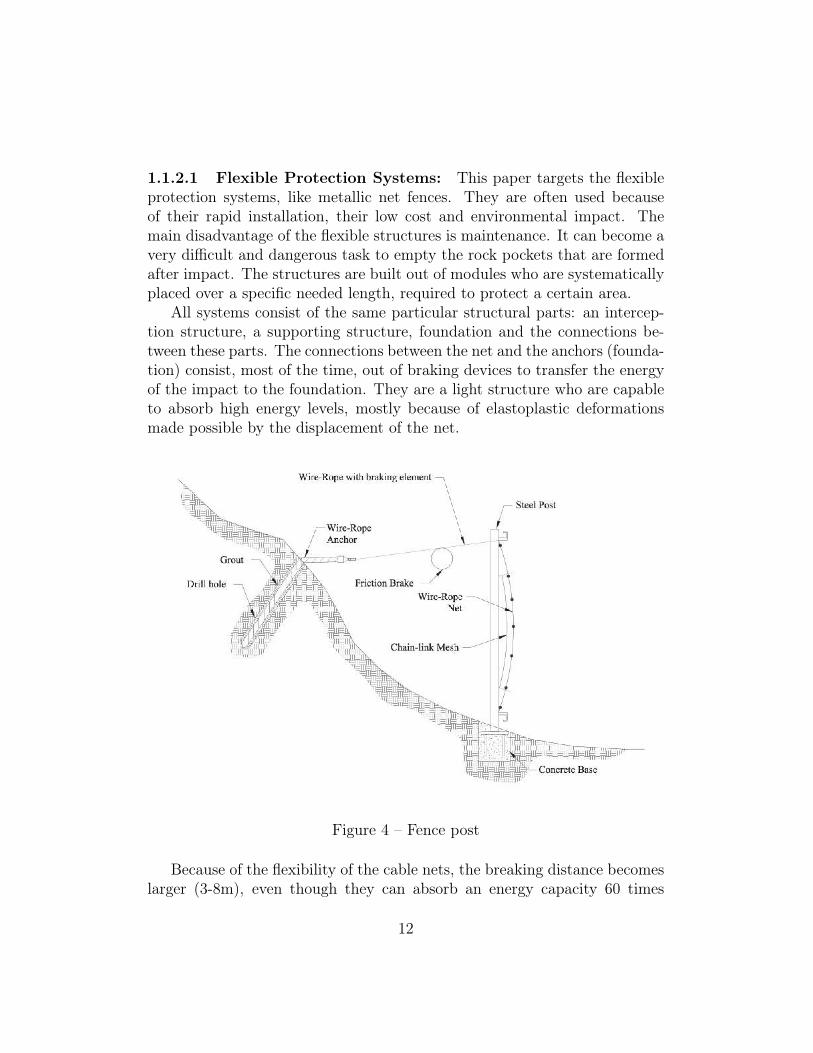
1.1.2.1 Flexible Protection Systems: This paper targets the flexibleprotection systems, like metallic net fences. They are often used becauseof their rapid installation, their low cost and environmental impact. Themain disadvantage of the flexible structures is maintenance. It can become avery difficult and dangerous task to empty the rock pockets that are formedafter impact. The structures are built out of modules who are systematicallyplaced over a specific needed length, required to protect a certain area.
All systems consist of the same particular structural parts: an intercep-tion structure, a supporting structure, foundation and the connections be-tween these parts. The connections between the net and the anchors (founda-tion) consist, most of the time, out of braking devices to transfer the energyof the impact to the foundation. They are a light structure who are capableto absorb high energy levels, mostly because of elastoplastic deformationsmade possible by the displacement of the net.
Figure 4 – Fence post
Because of the flexibility of the cable nets, the breaking distance becomeslarger (3-8m), even though they can absorb an energy capacity 60 times
12

bigger than with rigid barriers. Metallic nets are now capable of absorbing akinetic energy of 3000 kJ. With flexible systems, the boulder will be stoppedmore smoothly over a long breaking distance which leads to a reduction ofthe peak-loads in every component of the structure. The energy-absorbingcapacity has increased by a factor 10 over the last ten years due to all theresearch on this subject.
1.1.2.2 Certification: To know if metallic fences are fit for use, theymust comply with a European Technical Approval (ETA) if no correspond-ing standard exists. The ETA-document sets the basis for the certificationprocedure, which must be carried out by an approved body that has beenrecognized by the European Commission. Since no relevant standard ruleswere set for rockfall net fences, EOTA (European Organization for TechnicalApprovals) endorsed a new European Technical Approval Guideline (ETAG)called “Falling rock protection kits". In this guideline, a testing procedurefor CE-marking of net fences has been defined.
Standard fence testing guidelines test at two energy levels: Service EnergyLevel (SEL) and Maximum Energy Level (MEL). SEL represents the energycapacity (rating) a system can absorb after two impact tests and where nomaintenance is required. MEL represents the maximum energy capacity(rating) of a fence from a single impact where the sole purpose is to stopthe rock, regardless the condition of the fence. Standard testing proceduresrequire the MEL-value to be 3 times the SEL-value. When choosing a fence,consideration should be given to the frequency of the SEL and MEL rockfallimpacts as this will directly correspond to maintenance requirements andconstruction costs. For most typical highway rock cuts, designing for SEL issufficient.
This method of verification give engineers the ability to identify the rele-vant characteristics, identify the threshold of the values and define the rele-vant identification tests. The data obtained by these tests, can be combinedto achieve a robust design which includes the systematic use of partial safetyfactors. Because of the guideline, it is now possible to compare products onthe basis of the absorbed energy.
1.1.3 Conclusion
Because of the many advantages of metallic nets, the research for reliablemodels becomes a necessity. Due to the high costs of full-scale experiments,
13
numerical procedures are being developed and improved to provide low-cost-models of the net design. Simulations of the numerical models help to gaina better understanding of the dynamical behaviour of the protection systemand its components, during the impact of a boulder. Dimensional analysiswill be the tool to provide models that give an (almost) exact representa-tion of the necessary characteristics of the prototypes. Tests on these modelscontribute to valuable experimental data in a less expensive manner. Dimen-sional or similarity analysis defines the relation between model and prototype.
1.2 Dimensional or similarity analysis
Modelling : Reduces a complicated or complex structure, called a proto-type, to a significantly simpler structure without losing characteristics in thebehaviour.
Model (definition given by Murphy) : A model is a device which is sorelated to a physical system that observations on the model may be used topredict accurately the performance of a physical system in the desired respect.
Prototype (definition given by Murphy): The physical system for whichthe predictions are to be made is called the prototype.
As said in the definition of modelling, dimensional analysis providesa method to simplify a physical system (prototype) to a simpeler system(model) to obtain valid experimental data. Experiments applied on mod-els will reduce the number and costs of the experiments and give a betterunderstanding of the local and global behaviour of the system. In general,modelling is advisable when :
- The prototype is too small or too large
- The prototype is not accessible
- The magnitudes of variables on the prototype are too small or too largeto be measured
- Testing on the prototype would take too long or too short a time
14
Dimensional analysis provides a tool to reduce the number and complexityof experimental parameters that affect a given physical phenomenon. Eventhough it does not solve the problem, it suggests a strategy for choosing therelevant data for solving a problem and how it should be presented. If thevariables of a physical situation are identified, similarity analysis (same asdimensional analysis) makes it possible to form a relationship between them.When a valid model is successfully developed, it will be able to predict thebehaviour of a prototype under certain conditions.
Similarity: Two systems are similar if their corresponding variables areproportionally at corresponding locations and times. Requirements for sim-ilarity suggest that the nondimensional principle equations be the same andthat there is an equality of the nondimensional independent variables. In or-der to compare the results between model and prototype, physical similaritybetween the two must exist. Physical similarity can be divided into threetypes:
1. Geometrical Similarity:- Same shape- Linear dimensions on model and prototype correspond with constantscale factors
2. Kinematic Similarity:- Velocities at corresponding points on model are prototype differ onlyby a constant scale factor.
3. Dynamic Similarity:- Forces on model and prototype differ only by a constant scale factor.
1.3 Similitary methods in dynamic engineering
1.3.1 Model Law
Model laws provide a condition of similarity, were the relationship of differentvariables of prototype and model are equal. If the model law of a system isvalid, that means that prototype and model are similar. By definition: theModel Law is a relation, or a set of relations, among scale factors relevant toa particular modelling instance. A scale factor is the ratio of the magnitudesof that variable for the prototype and its model. Even though there may
15
be more than one relation among scale factors, there is only one ModelLaw. The Model Law is the principal tool in the design of a modellingexperiment. A Model Law can often be used to compare the behaviour andgeneral performance of existing, or even hypothetical, systems. In thesecases, of course, comparisons can be done without constructing a “model”or carrying out tests. The determination of a Model Law, or the relationbetween the scaling factors, are described in Baker et al in two differentways.
1. Application of Partial Differential Equations : the researcher must havea sufficient amount of knowledge about the physics of the problem tobe able to write down a set of differential equations. It gives a goodrepresentation of the physical meaning of the system.
2. Buckingham Pi-theorem : the relations between the variables are equalfor model and prototype and where no specific knowledge of the systemis necessary. This will be used for complex systems where the numberof parameters has to be reduced to simplify the system.
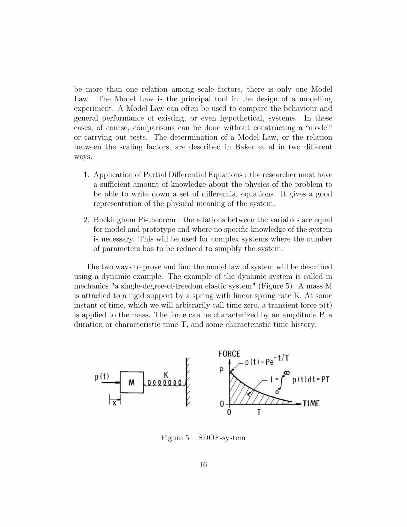
The two ways to prove and find the model law of system will be describedusing a dynamic example. The example of the dynamic system is called inmechanics "a single-degree-of-freedom elastic system" (Figure 5). A mass Mis attached to a rigid support by a spring with linear spring rate K. At someinstant of time, which we will arbitrarily call time zero, a transient force p(t)is applied to the mass. The force can be characterized by an amplitude P, aduration or characteristic time T, and some characteristic time history.
Figure 5 – SDOF-system
16
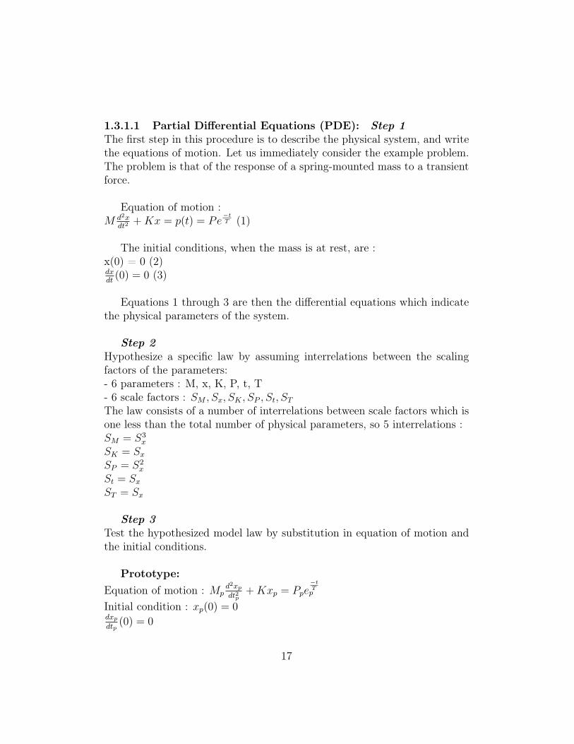
1.3.1.1 Partial Differential Equations (PDE): Step 1
The first step in this procedure is to describe the physical system, and writethe equations of motion. Let us immediately consider the example problem.The problem is that of the response of a spring-mounted mass to a transientforce.
Equation of motion :M d2x
dt2+Kx = p(t) = Pe
−tT (1)
The initial conditions, when the mass is at rest, are :x(0) = 0 (2)dxdt(0) = 0 (3)
Equations 1 through 3 are then the differential equations which indicatethe physical parameters of the system.
Step 2
Hypothesize a specific law by assuming interrelations between the scalingfactors of the parameters:- 6 parameters : M, x, K, P, t, T- 6 scale factors : SM , Sx, SK , SP , St, ST
The law consists of a number of interrelations between scale factors which isone less than the total number of physical parameters, so 5 interrelations :SM = S3
x
SK = Sx
SP = S2x
St = Sx
ST = Sx
Step 3
Test the hypothesized model law by substitution in equation of motion andthe initial conditions.
Prototype:
Equation of motion : Mpd2xp
dt2p+Kxp = Ppe
−tTp
Initial condition : xp(0) = 0dxp
dtp(0) = 0
17

Model:Equation of motion : Mm
d2xm
dt2m+Kxm = Pme
−tTm
Initial condition : xm(0) = 0dxm/dtm(0) = 0
Step 4
Prove or disprove the invariance of the substitution from previous step, byuse of the proposed model law.Here in this example : Sx = SMm = S3Mp
xm = Sxp
tm = StpTm = STp
Km = SKp
Pm = S2Pp
After substitution in the equation of motion of the model:
Model:Equation of motion : S3Mp(
Sd2xp
S2dt2p) + SKpSxp = S2Ppe
−Stp
STp
After cancellation of S : Mp( xp
dt2p+Kpxp = Ppe
−tp
Tp
Initial conditions :Sxp(0) = 0Sdxp
Sdtp(0) = 0
Cancellation of S:xp(0) = 0dxp
dtp(0) = 0
Equations 1 through 3 are invariant under the change of prototype tomodel, thus the model law is proven.
1.3.1.2 π-Buckingham or Vaschy-Buckingham theorem As explainedearlier, the Buckingham Pi-theorem is a tool used to find dimensionless prod-ucts of relevant parameters that allow to express a physical relationship be-
18

tween model and prototype. These dimensionless products will be calledpi-terms.
The behaviour of a physical system is defined by the complete set of di-mensionless variables formed by the relevant physical variables. This factsuggests that if two systems have the same numerical values for all dimen-sionless variables, then these two systems are dimensionally similar. Further,if model and prototype are dimensionally similar, there behaviour can beclosely correlated. This is the essence of dimensional modelling. Therefore,the first step in a model experiment is to construct the complete set of di-mensionless variables relevant to the system. The Buckingham Pi-theorem isthe most popular manner to find dimensionless variables and will be appliedin this project.
The theorem loosely states that if we have a physically meaningful equa-tion involving a certain number n, of physical variables, and these variablesare expressible in terms of k independent fundamental physical quantities.The original expression is equivalent to an equation involving a set of p (isequal to n - k) dimensionless parameters constructed from the original vari-ables.
To prove the model law we must first find the dimensionless parametersof the problem.The variables of the problem are : M, x, K, P, T (n)The primary dimensions are : M, T, L (k)This means that there will be n-k = 2 pi-terms (dimensionless parameters)The equation of dimensional homogeneity states:M0L0T0 = Xa1Ka2Ma3P a4T a5
Rewrite the variables in function of the primary dimensions:M0L0T0 = La1(M
T 2 )a2Ma3(ML
T 2 )a4T a5
M0L0T0 = La1+a4Ma2+a3+a4T−2a2−2a4+a5
Equate exponents to get zero :M : a2 + a3 + a4 = 0L : a1 + a4 = 0T : −2a2 − 2a4 + a5 = 0
In function of a1 and a5 :a2 =
1
2a5 + a1
a3 = −1
2a5
19

a4 = −a1
M0L0T0 = Xa1K1
2a5+a1M
−1
2a5P−a1T a5
M0L0T0 = (XKP
)a1(
√
K
MT )a5
The dimensionless parameters of this problem are:
π1 =XKP
and π2 =√
KMT
To achieve dimensional similarity between model and prototype, the di-mensionless parameters must be equal :
π1 :XmKm
Pm= XpKp
Pp⇒ Xm
Xp
Km
Kp= Pm
Pp
π2 :
√Km
Mm
Tm =
√
Kp
Mp
Tp ⇒ (Km
Kp)(Tm
Tp)2 = Mm
Mp
If now :Sx = Xm
Xpis the distance scale factor
SK = Km
Kpis the spring scale factor
SM = Mm
Mpis the mass scale factor
ST = Tm
Tpis the time scale factor
SP = Pm
Ppis the amplitude scale factor
According to the pi-terms, the model law states :Sx.Sk = SP
SK .S2T = SM
The downside of using partial differential equations is that the researchermust have a sufficient amount of knowledge about the physics of the problemto be able to write down a set of differential equations. This is also thereason why PDE isn’t a popular method for obtaining model laws. Findingdimensionless parameters using the Buckingham theorem is common for morecomplex structures. The downside of this method is the lack of physicalmeaning describing the structural problem.
20

1.4 Similarity Applications
Different kinds of methods are used to achieve similarity relationships be-tween model and prototype, as described above. Two similarity applicationswho are widely used and were discussed in Baker et al. (1991), will be ex-plained here due to their high importance.
1.4.1 "Replica" modeling :
A replica is a model of a dynamic system or structure of exactly the samegeometry and materials as a prototype, but scaled in size alone. Only the lin-ear dimensions on model and prototype are scaled down or up with constantscale factors
1.4.2 "Dissimilar material" modeling :
The second approach is the "dissimilar material"modelling. Dissimilarmaterial models are models that are made of materials differing from thosein the prototype, but possessing constitutive similarity. This means that thematerial of the model has homologous (‘in relation to’) properties and stress-strain curves as the ones of the prototype. Materials possessing constitutivesimilarity will have identical scaled strength and stiffness properties so thatthe dimensionless stress is identical for all strains. Material properties withdimensions of stress, which is used to normalize the curve can be : Young’smodulus E, yield stress σy and ultimate stress σu. An example of dimension-less stress-strain curves for materials which are deformed well into the regionof plastic deformation is shown in Figure 6.
Figure 6 – Stress-Strain curves
The use of dissimilar material models allows additional freedom in bothstatic and dynamic model testing of structures, beyond the possibilities with
21
replica models. Because of this method, for example, tests can be done onmodels who consist of cheaper or ’easier’ materials and who are still able todeliver accurate experimental data.
Similarity methods, more specifically "replica" modelling, will be pro-posed in this research for the design of metallic fences as rockfall protectionsystems. To sum up, a few advantages of similarity applications are givenbelow:
1. to obtain experimental data for quantitative evaluation of a particulartheoretical analysis;
2. to explore the fundamental behaviour involved in a little understoodphenomenon;
3. to obtain quantitative data for use in prototype design problems, par-ticularly when mathematical theory is overly complex or even non-existent;
4. to generate a functional relationship empirically to solve a general prob-lem;
5. to evaluate limitations for an expensive system already in existence.
1.4.3 Example : Droptest
The two methods will be shown using an example : "Drop Test" describedin Baker et al. (1991)
22

(a) Set-up experiment
(b) Characteristics experiment
Figure 7 – Droptest
The drop test device consists of drop masses which will fall freely downa guide rod to impact on a spring at the bottom of the guide (Figure 7a).On impact with the spring, the masses rebound with a very rapid changein velocity. Any light structure attached to the drop mass experiences asevere deceleration pulse during impact which is transmitted to the struc-ture through its point of attachment. The particular structures used in thedemonstration experiments were slender cantilever beams of steel and alu-minum alloy.
- Prototype : a 1015/1018 strip of steel with a free length of 5.0 inches,a width of 0.25 inch, and a thickness of 0.020 inch.
- Model : a 5052-0 aluminum strips twice as large in all dimensions asthe prototype beams.
23

All characteristics can be found in the table presented in Figure 7b. Us-ing replica modelling would only scale the dimensions geometrically andleave the material properties untouched. Using dissimilar material mod-elling we change the geometry and the properties of the material by using another metal. By drop testing these cantilever beams from different heights,the beams experienced various amounts of permanent deformation. Figure8 shows a group of deformed model and prototype cantilever beams. Thedeformed shapes of both model and prototype systems are geometricallysimilar.
Figure 8 – Deformed prototypes and models
Dimensional plots of the variation in residual tip deformation, are shownin Figure 9 . This unsealed plot gives no indication that the aluminum andsteel systems of beams are truly equivalent ones. Obviously, a steel beamwhich is only 5 inches long cannot deflect 8 inches as do some of the 10-inch long aluminum beams. Such plots can be much more valuable whenmade non-dimensional. Figure 9 is a plot of scaled or normalized tip deflec-tion as a function of scaled or normalized drop height. Both systems giveidentical non-dimensional tip deformations as a function of non-dimensionaldrop height. The students who conduct these tests demonstrate how resultsfrom experiments on one system can predict results for another system. Even
24

though the materials are different in each set of beams, and the lengths ofbeams differ, a comparison of permanent deformations from the two.
Figure 9 – Dimensional and non-dimensional results
2 Methodology
2.1 Introduction
The main idea is to explore the potentiality of dimensional analysis (alsocalled similarity analysis) to propose a cost effective prototype (at a reducedscale) allowing a preliminary experimental testing of the structure technol-ogy and reduce the number of full scale tests necessary to validate the newproduct.
25
The method that has been discussed earlier will now be applied on therockfall protection system. After using dimensional analysis, it will be pos-sible to create a model wherein numerical experiments will be tested. Theresults of these experiments lead to a good representation of a prototype ofa structure that will be able to stop falling boulders in several different con-ditions. In order to design the model, the protection system will be dividedinto several components using a step-by-step approach. The first step of thisapproach contains tests that happen on a cable-scale. Afterwards, the exper-iments grow in complexity to eventually arrive at the total structure. Thestitch-scale offers a small section of the mesh where a couple of forces will beimplemented.
All data needed to built dimensionless relationships will be producedeither by analytical approaches or by DEM simulations.
2.2 Cable scale
2.2.1 Cable Structure
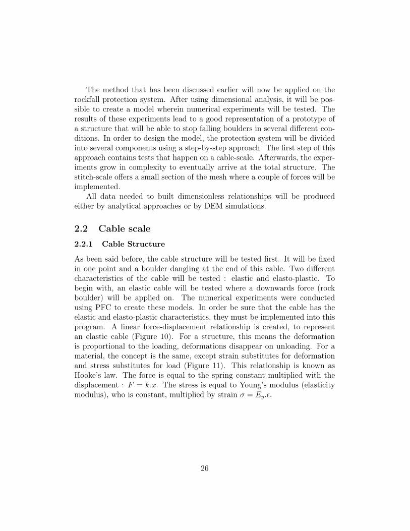
As been said before, the cable structure will be tested first. It will be fixedin one point and a boulder dangling at the end of this cable. Two differentcharacteristics of the cable will be tested : elastic and elasto-plastic. Tobegin with, an elastic cable will be tested where a downwards force (rockboulder) will be applied on. The numerical experiments were conductedusing PFC to create these models. In order be sure that the cable has theelastic and elasto-plastic characteristics, they must be implemented into thisprogram. A linear force-displacement relationship is created, to representan elastic cable (Figure 10). For a structure, this means the deformationis proportional to the loading, deformations disappear on unloading. For amaterial, the concept is the same, except strain substitutes for deformationand stress substitutes for load (Figure 11). This relationship is known asHooke’s law. The force is equal to the spring constant multiplied with thedisplacement : F = k.x. The stress is equal to Young’s modulus (elasticitymodulus), who is constant, multiplied by strain σ = Ey.ǫ.
26

Figure 10 – Elastic : Force-displacement graph
Figure 11 – Elastic : Stress-Strain graph
Elasto-plastic character of a material can be described as the defor-mation of a (solid) material undergoing non-reversible changes of shape inresponse to applied forces. As seen on Figure 12, the curve first describes anelastic deformation until the load exceeds a threshold – the yield strength.The extension increases more rapidly than in the elastic region.
27
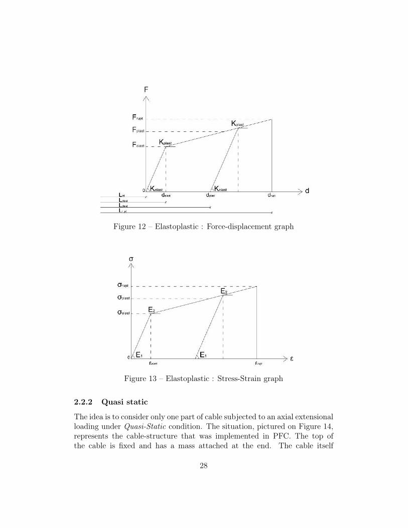
Figure 12 – Elastoplastic : Force-displacement graph
Figure 13 – Elastoplastic : Stress-Strain graph
2.2.2 Quasi static
The idea is to consider only one part of cable subjected to an axial extensionalloading under Quasi-Static condition. The situation, pictured on Figure 14,represents the cable-structure that was implemented in PFC. The top ofthe cable is fixed and has a mass attached at the end. The cable itself
28

is divided into N strands or particles, with an equal distance between oneanother, who represent the force interaction that happens throughout thecable. This way it is possible to form elastic and elasto-plastic characteristicsby manipulating the forces that work between the particles. During the firstcondition we will analyse the quasi static condition where only gravity willbe an applied external force on the boulder. The main parameters of interestare given in the Table 1 . In the elasto-plastic cable several extra variablesare implemented like the stress and strain in plastic conditions. To find thedimensionless parameters (π-terms), all the important variables are writtenusing 3 fundamental dimensions namely M, T, L. As seen in the Buckinghamtheorem this will lead to 3 π-terms for the elastic cable and 6 pi-terms forthe elasto-plastic cable. pi2const
Figure 14 – Scheme Quasi-Static condition
29

Table 1 – Table of properties QS condition : Cable-Scale
30

2.2.3 Dynamic
In the dynamic condition we introduce an extra parameter : the drop height,from which the boulder is released (Figure 15). To add this extra variableand to not change the structure of the system, an external downwards veloc-ity vi was introduced, working on the boulder. This velocity was written asa function of the height :
Ek = Ep1
2Mb.v
2i = Mb.g.Hb
→ vi =√2.g.Hb
Again the dimensions were written next to every parameter in table 2.This leads to 4 dimensionless parameters for the elastic cable and 7 dimen-sionless parameters for the elasto-plastic cable.
Figure 15 – Scheme Dynamic condition
31

Table 2 – Table of properties Dynamic condition : Cable-Scale
32

2.2.4 pi-terms derivation
Using the Buckingham Pi-theorem, explained earlier with the SDOF model,it was possible to find the π-terms in every condition (Table 3). After verify-ing that the π-terms are indeed dimensionless and independent, the processto find interesting relations between the variables can begin.
Table 3 – Table of pi-terms : Cable-Scale
2.3 Stitch scale
2.3.1 Stitch Structure
After finishing the working method on cable-scale, the researched structurewill grow in complexity, as explained in the introduction of the methodol-ogy. The second part of the experiments focusses on the stitch-scale, whichrepresents a smaller area of the mesh. The model of the stitch structureconsists of particles that represent the different connections of the net. Somerepresent clips that allow the cable to slide, this helps to absorb the shockduring impact. Others maintain the attachment with other cables. All theproperties of the connections (or particles) are defined in the model, as wellas their behaviour with neighbouring particles. The size of a net structure
33
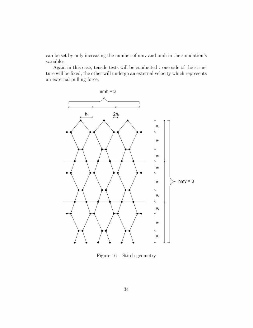
can be set by only increasing the number of nmv and nmh in the simulation’svariables.
Again in this case, tensile tests will be conducted : one side of the struc-ture will be fixed, the other will undergo an external velocity which representsan external pulling force.
Figure 16 – Stitch geometry
34

2.3.2 pi-terms derivation
Dimensional analysis will be used to describe the effect of the geometry inwhich the cables are placed and connected with one another. The importantgeometry variables are given in the Table 4, they will define the shape andthe proportions of the net. The objective of the stitch structure, compared tothe cable-structure, is to focus the attention on the geometry. Experimentswill be done by changing the variables of the geometry while keeping theremaining variables constant. Afterwards it will (hopefully) be possible toshow the effect that geometry variations have on the strength and elongationof the structure.
Table 4 – Table of properties : Stitch-Scale
The table below (Table 5) shows the different π-terms that were found
35
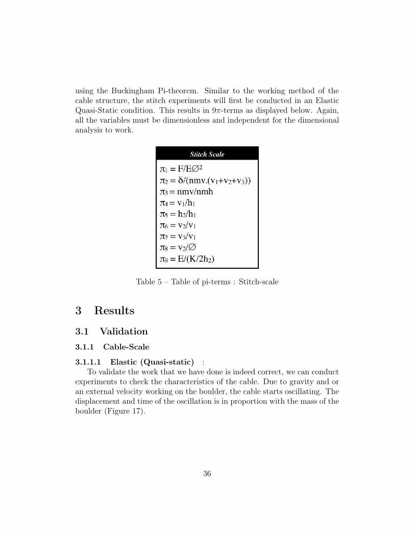
using the Buckingham Pi-theorem. Similar to the working method of thecable structure, the stitch experiments will first be conducted in an ElasticQuasi-Static condition. This results in 9π-terms as displayed below. Again,all the variables must be dimensionless and independent for the dimensionalanalysis to work.
Table 5 – Table of pi-terms : Stitch-scale
3 Results
3.1 Validation
3.1.1 Cable-Scale
3.1.1.1 Elastic (Quasi-static) :To validate the work that we have done is indeed correct, we can conduct
experiments to check the characteristics of the cable. Due to gravity and oran external velocity working on the boulder, the cable starts oscillating. Thedisplacement and time of the oscillation is in proportion with the mass of theboulder (Figure 17).
36
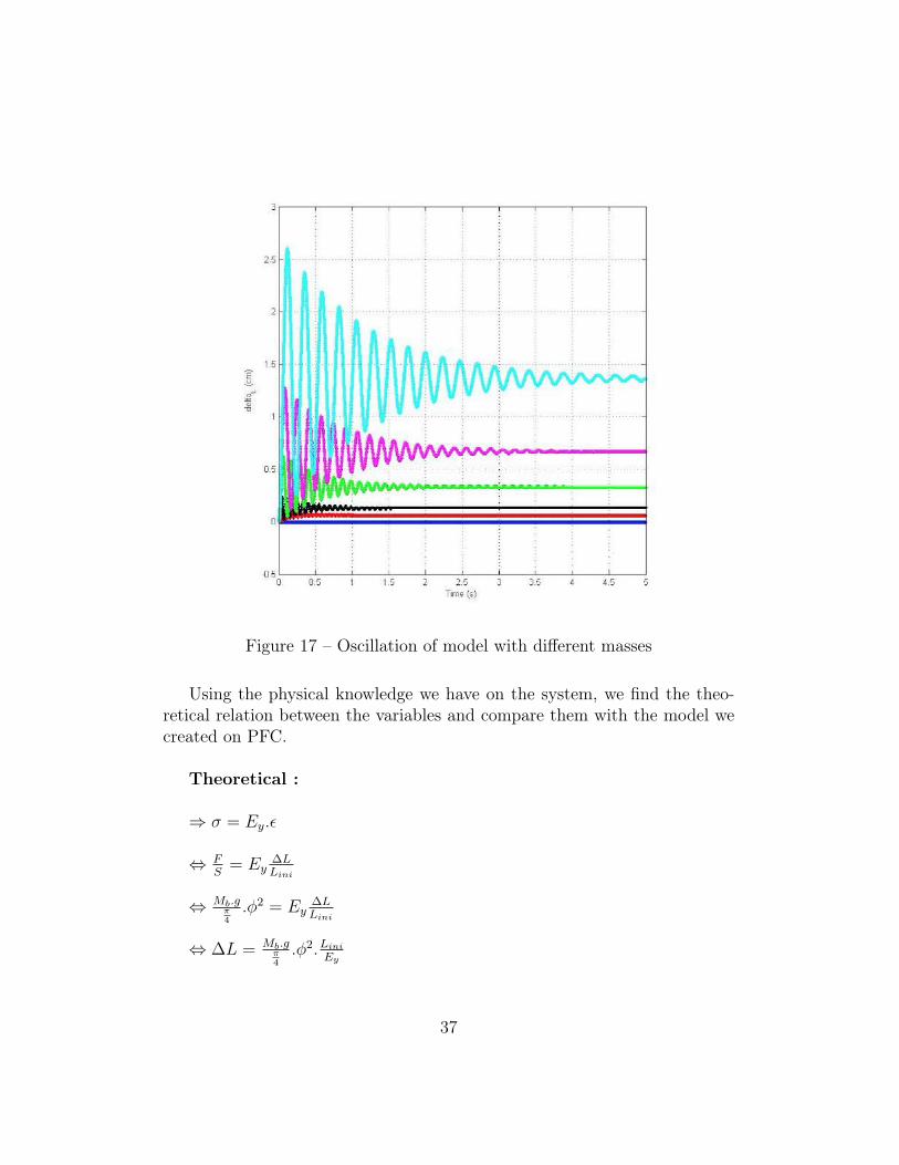
Figure 17 – Oscillation of model with different masses
Using the physical knowledge we have on the system, we find the theo-retical relation between the variables and compare them with the model wecreated on PFC.
Theoretical :
⇒ σ = Ey.ǫ
⇔ FS= Ey
∆LLini
⇔ Mb.gπ4
.φ2 = Ey∆LLini
⇔ ∆L = Mb.gπ4
.φ2.Lini
Ey
37

The graph shows that for different masses (different forces), the theoret-ical and numerical model are describing the same elongation of the cable ina linear manner (Figure 18) which validates the model for an elastic cable inQS-condition.
Figure 18 – Validation of QS-Elastic behaviour
3.1.1.2 Elastic (Dynamic) : The elastic cable in a dynamic situationhas been verified by comparing a theoretical SDOF-model, using the sameparameters(mass of boulder, length cable, elasticity module, ...) as the PFC-model. To be sure to show the dynamic effect of the boulder, the simulationstarts oscillating in a Quasi-Static condition until it reaches its equilibrium.In a second phase, the drop height of the boulder initiates a dynamic condi-tion. This causes an oscillation with a bigger displacement (Figure 19).
38
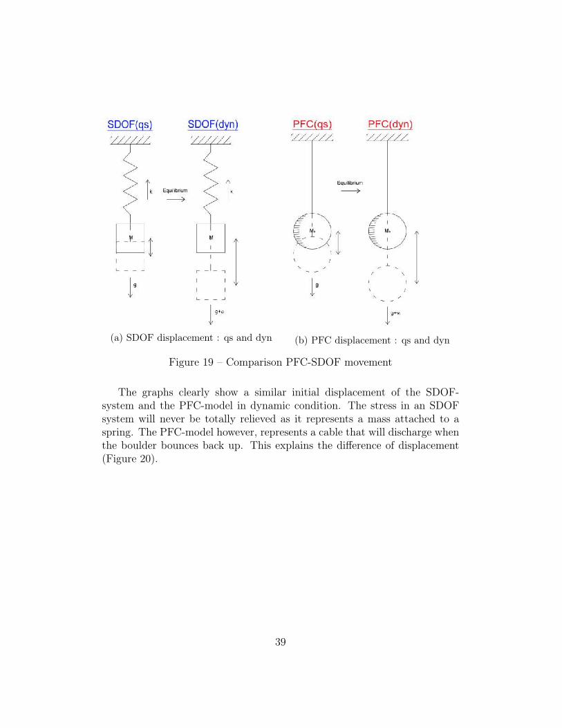
(a) SDOF displacement : qs and dyn (b) PFC displacement : qs and dyn
Figure 19 – Comparison PFC-SDOF movement
The graphs clearly show a similar initial displacement of the SDOF-system and the PFC-model in dynamic condition. The stress in an SDOFsystem will never be totally relieved as it represents a mass attached to aspring. The PFC-model however, represents a cable that will discharge whenthe boulder bounces back up. This explains the difference of displacement(Figure 20).
39

(a) Transition QS-Dyn (b) Dynamic SDOF-PFC
Figure 20 – Validation of PFC model compared to SDOF-system
3.1.1.3 Elasto-plastic (Quasi-static) :The validation of the elastoplastic character of the cable will be divided
into an elastic and plastic region. The two forces representing the behaviourare defined below : F1 represents the force working during elasticity and F2
represents the force during plasticity.To clarify (!) : In this section the words ’Quasi-Static’ and ’Dynamic’ willrefer to the oscillation of the boulder. ’Quasi-static’ will refer to a displace-ment of the boulder after achieving equilibrium, ’Dynamic’ will refer to themaximal displacement that the oscillation achieves. These two terms do notrefer whether or not an extra force/drop height is applied on the boulder,the boulder remains in Quasi-Static condition.
Elastic:F1 = k.x with xǫ[0, de]
Plastic:F2 = k′(x− de) + Fe with xǫ[de, dr]
40

The exterior work applied on the structure is equal to the kinetic energyplus the interior work, that represents the elastoplastic character of the cable.In the Quasi-Static condition, the kinetic energy will be zero since no externalforce will be implemented on the cable (except for gravity).
∆Ec +∆Wint = ∆Wext
∆Ec =1
2.Mb.∆v2 = 0
∆Wext = Mb.g.x∆Wint = ∆Wdiss +∆Wdefo
Figure 21 – Force-Displacement
In the elastic region (before plasticity occurs) for a Dynamic displace-ment we can state that :
i.e. δDyǫ[0, de]
∆Ec+∆Wint = ∆Wext where
∆Ec = 1
2.m(v2f − v2i ) = 0
41

∆Wint =∫ δDy
0δW1
or δW1 = k.x.dx⇔ ∆Wint =
1
2.k.δ2Dy
∆Wext = Mb.g.δDy
⇒ 1
2.k.δ2Dy = Mb.g.δDy
⇔ δEDy =2.Mb.g
k
For the Quasi-Static situation we can state that:
⇒ σ = Eǫ⇔ F
S= E
δQS
L
⇔ δEQS = Mb.g
k
This means : ⇔ δEDy = 2.δEQS
This has to be understood to interpret the right results coming from the
PFC-model. Felast will be reached with a mass Mb =Melast
b
2, i.e. half of
the QS-load (M elastb ). The graph below (Figure 22b) shows a simulation of
the PFC-model where the elongation of the cable is calculated in function oftime. It clearly shows that the oscillation reaches 2cm, using a mass Mb inDynamic condition and 1cm (δQS =
δDy
2⇔ 2cm
2) in Quasi-Static condition.
Theoretical Results:
Properties of the model :Ey = 250.109Paφcab = 10−3mL = 10mσelast = 500.106Paσrupt = 700.106PaM elast
b = 4003, 05kgM rupt
b = 5604, 27kgǫrupt = 0, 015
Calculations :
42

delast = L.ǫelast = L.σelast
Ey= 0, 02m
Felast = σelast.π4.φ2 = 39, 27kN
Frupt = σrupt.π4.φ2 = 54, 98kN
drupt = L.ǫrupt = 0, 15m
(a) Scheme displacement (b) Result QS-Dyn
Figure 22 – QS-Dynamic Displacements in elastic region
In the plastic region :
i.e. δDyǫ[de, dr]
∆Wint =∫δW with δW = F.dx
∆Wint =∫ δDy
0δW =
∫ de
0δW1 +
∫ δDy
deδW2 = I1 (elastic) + I2(plastic) with
δW1 = F1.dx = k.x.dxδW2 = F2.dx = k′(x− de) + Fe
43

I1 =∫ de
0k.x.dx = 1
2.k.de2 which will be called the Elastic region
I2 =∫ δDy
de(k′(x− de) + Fe).dx
= [k′(x2
2− de.x) + Fe.x]
δDy
de
= [k′.x2
2+ (Fe− k′.de)x]
δDy
de
= k′
2(δ2Dy−de2)+(Fe−k′de)(δDy−de) which will be called the Plastic region
⇔ ∆Wint =k′
2(δ2Dy − de2) + (Fe− k′de)(δDy − de) + 1
2.k.de2
Wdefo =1
2.FDy.(δDy − δperm) with
FDy(δDy) = k′(δDy − de) + Fe
K =FDy
δDy−δperm⇔ δperm = δDy −
FDy
K
⇔ Wdefo =1
2.FDy.
FDy
K= 1
2.K.F 2
Dy
⇔ ∆Wdefo =1
2K.[k′(δDy − de) + Fe]2
=⇒ Wdiss = ∆Wint − Wdefo
(a) W interior (b) Deformed W
Figure 23 – QS-Dynamic Displacements in elastic region
44

∆Ec = 0(vi = 0, vf = 0) where ∆Wint = ∆Wext
⇔ k′
2(δ2Dy − de2) + (Fe− k′.de)(δDy − de) + 1
2.k.de2 = Mb.g.δDy
⇔k′
2︸︷︷︸
δ2Dy + (Fe− k′de−Mb.g)︸ ︷︷ ︸
.δDy +1
2(k + k′).de2 − Fe.de
︸ ︷︷ ︸
= 0
⇔ a.δ2Dy + b.δDy + c = 0
This makes it possible to calculate δDy.
The theoretical results in Figure 24 are divided in an elastic and plasticelongation of the cable. Comparing the results shown in the calculations, itis possible to observe del as the intersection between the two curves, which is0.02m. The coloured grey area represents the elastic zone of the calculations.The PFC-model follows the elastic curve until it reaches delast and continueson the plastic curve, thus representing elasto-plastic behaviour. In Figure 25it is also shown that pfc-results correspond to the theoretical results : Felast
(39,27kN) is reached at delast. One value however doesn’t follow the samecurve as previous results (blue circle). This is due to the applied force whichcauses the cable to break, known as Frupture which has a value of 54,98kN.The forces that work on the cable will not surpass this value and the curvewill be horizontal from thereon. These results show the validation of themodel in elastoplastic-qs condition.
45

Figure 24 – QS Elastopl : Mass-Elongation
46

Figure 25 – QS Elastopl : Force-Displacement
3.1.1.4 Elasto-plastic (Dynamic) :The method of working will be similar as described in QS-situation :
∆Ec +∆Wint = ∆Wext
∆Ec =1
2.Mb.∆v2
∆Wext = Mb.g.x∆Wint = ∆Wdiss +∆Wdefo
However, ∆Ec will not be equal to zero because now an initial speed isimplemented to the model. This velocity represents the drop height fromwhich the boulder falls down, it will be written as a function of the imple-mented height : vi =
√2.g.Hb
The different colors exhibit the theoretical results, found with different masses.The displacement of all the curves does not start at zero since an elongation
47

already has taken place in QS-condition. The graph (Figure 26) shows thatthe PFC model (circles) presents a similar output compared to the theoret-ical curves. The grey area represents (again) the elastic region of the cable,ending at a displacement of 0,02m.
Figure 26 – Dynamic Elastopl : Validation
3.1.2 Stitch-Scale
3.1.2.1 Elastic (Quasi-static) :
48
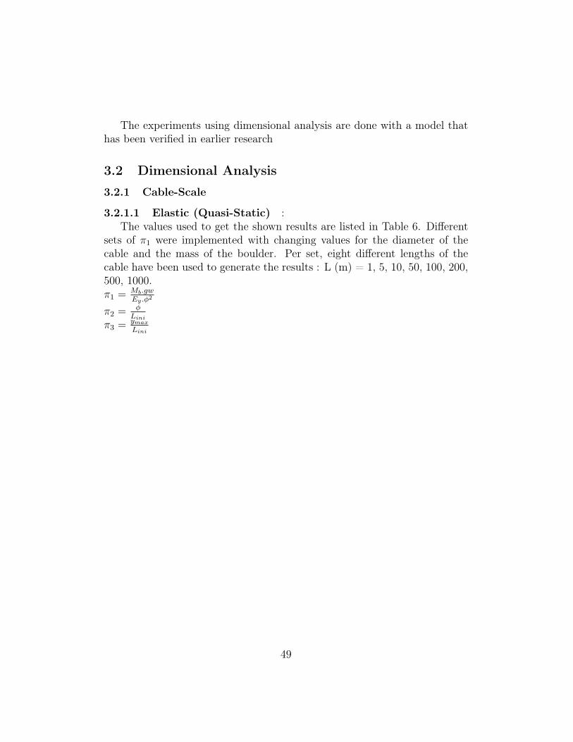
The experiments using dimensional analysis are done with a model thathas been verified in earlier research
3.2 Dimensional Analysis
3.2.1 Cable-Scale
3.2.1.1 Elastic (Quasi-Static) :The values used to get the shown results are listed in Table 6. Different
sets of π1 were implemented with changing values for the diameter of thecable and the mass of the boulder. Per set, eight different lengths of thecable have been used to generate the results : L (m) = 1, 5, 10, 50, 100, 200,500, 1000.π1 =
Mb.gw
Ey .φ2
π2 =φ
Lini
π3 =ymax
Lini
49
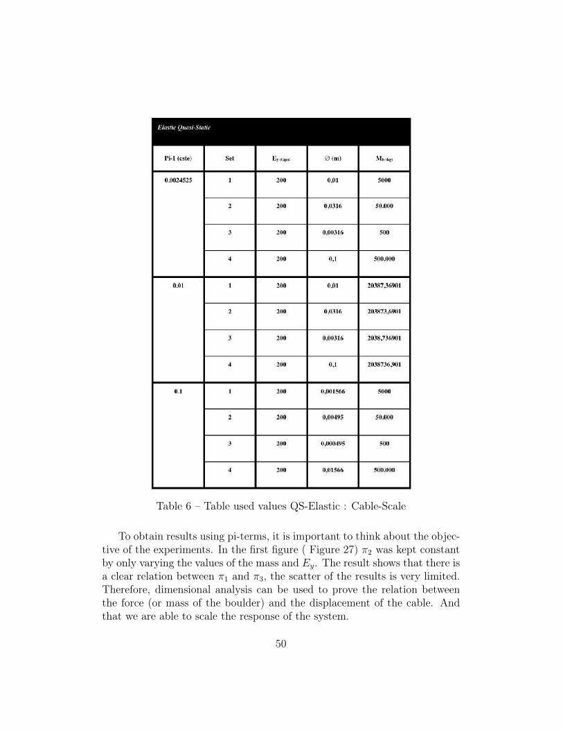
Table 6 – Table used values QS-Elastic : Cable-Scale
To obtain results using pi-terms, it is important to think about the objec-tive of the experiments. In the first figure ( Figure 27) π2 was kept constantby only varying the values of the mass and Ey. The result shows that there isa clear relation between π1 and π3, the scatter of the results is very limited.Therefore, dimensional analysis can be used to prove the relation betweenthe force (or mass of the boulder) and the displacement of the cable. Andthat we are able to scale the response of the system.
50

Theoretically this can be written as :
⇒ σ = Ey.ǫ
⇔ FS= Ey
ymax
Lini
⇔ Mb.gπ4
.φ2 = Eyymax
Lini
⇔ Mb.gπ4
.φ2.Lini
Ey= ymax
with π1 =Mb.g
Eyand π3 =
ymax
Lini
The relationship between the dimensionless parameters becomesπ1 = π3.
π4
Figure 28 shows the results in function of π2 and π3. We can concludethat π2 and π3 work independent from each other.
Figure 27 – QS-Elastic : Relation pi1-pi3 (pi2= cst)
51

Figure 28 – QS-Elastic : Relation pi2-pi3 (pi1= cst)
3.2.1.2 Elastic (Dynamic) :The results of the modulation in Dynamic situation of an elastic cable are
shown in the Figure 29. π3 contains a fixed value with L and φ differing invalue, as seen in the table. The graph shows the transition from quasi-staticto dynamic by increasing the value of π2, in other words : increasing thedrop height.A low drop height results in gravity causing the displacement of the cable.When increasing the drop height we notice that the effect of gravity becomesnegligible, we call this the Dynamic situation. The dotted lines representthe theoretical values for the QS (equilibrium) and Dyn (max displacement)results. In QS-condition this means that π1 = π
4.π3. In Dynamic condition
this means that π1 = 2.π4.π3 because the displacement will be twice the value
as that of the QS result (δEDynam = 2.δEQS). A small drop height results intoa small value for π2 (green values) and reproduces a practically linear curvewith an angle of 2.π
4, which follows the theoretical result in Dynamic condi-
52
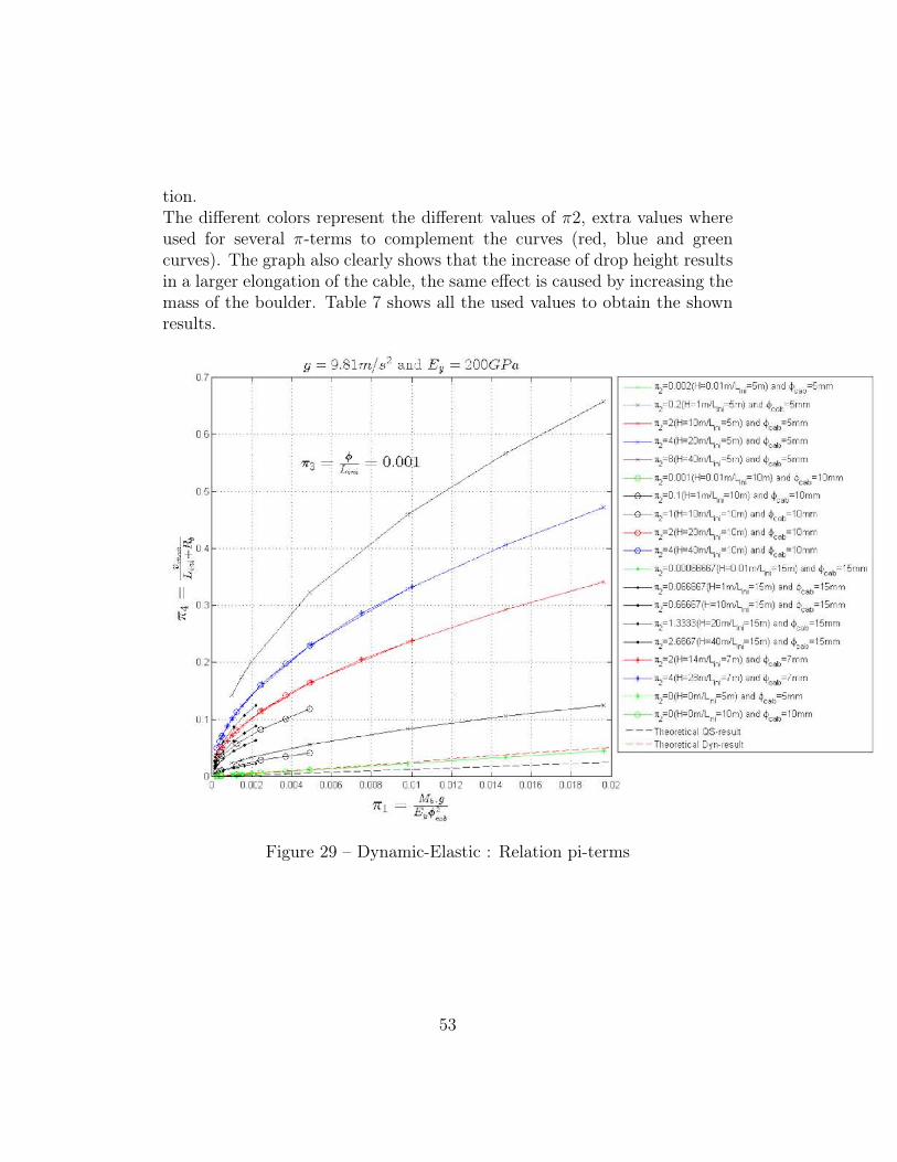
tion.The different colors represent the different values of π2, extra values whereused for several π-terms to complement the curves (red, blue and greencurves). The graph also clearly shows that the increase of drop height resultsin a larger elongation of the cable, the same effect is caused by increasing themass of the boulder. Table 7 shows all the used values to obtain the shownresults.
Figure 29 – Dynamic-Elastic : Relation pi-terms
53

Table 7 – Table used values Dyn-Elastic : Cable-Scale
3.2.1.3 Elasto-plastic(Dynamic) :Figure 30 shows an example with the following variables :
Mb = 10kgg = 9, 81m/sH = 1mL = 10mφ = 0, 01m
54
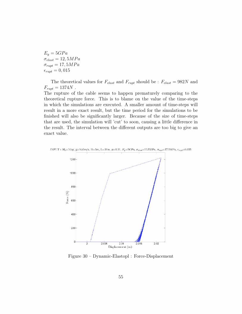
Ey = 5GPaσelast = 12, 5MPaσrupt = 17, 5MPaǫrupt = 0, 015
The theoretical values for Felast and Frupt should be : Felast = 982N andFrupt = 1374N .The rupture of the cable seems to happen prematurely comparing to thetheoretical rupture force. This is to blame on the value of the time-stepsin which the simulations are executed. A smaller amount of time-steps willresult in a more exact result, but the time period for the simulations to befinished will also be significantly larger. Because of the size of time-stepsthat are used, the simulation will ’cut’ to soon, causing a little difference inthe result. The interval between the different outputs are too big to give anexact value.
Figure 30 – Dynamic-Elastopl : Force-Displacement
55

The results of the π-term relations produces one curve (Figure 31) ofdifferent input-values. As seen in the table 8, π1, π2, π3 stay constant withwhich we change the values of the mass, E, σel and σrupt proportionally. Thedifferent simulations depend on the different drop heights : H(m) = 0.001,0.2, 0.3, 0.4, 0.5, 0.6, 0.7, 0.8, 0.9, 1.0, 1.1, 1.2, 1.3, 1.4. If the mass becomestoo small the curve will deviate from the predicted result. The reason for thisphenomenon remains unknown since the ratio’s of Mass, E, σelast and σrupt
remain constant. The graph (Figure 31) shows the relation between π6 andπ4, resulting in an almost linear effect of the drop height on the elongationof the cable, after achieving plasticity (above grey area).
Table 8 – Table used values Dyn-Elastoplastic : Cable-Scale
56

Figure 31 – Dynamic-Elastopl : Relation pi-terms
57

3.2.2 Stitch-Scale
3.2.2.1 Elastic (Quasi-static) :The objective of the experiments on stitch-scale were to see the effects
of the geometry on the force/displacement of the structure. The π-termsdidn’t allow changes on the geometric variables without changing materialproperties. After changing the number of repetitions of nmv and nmh andkeeping π3 constant, the result showed several different curves.This odd resultwas not explained during this research. The reason could be the choiceof the pi-terms, still it is strange that even though the pi-terms are non-dimensional, independent and constant (same ratio for π3) it gives a ’wrong’result. A conclusion could be that Replica-modelling will not be possibleon the structure. IF the characteristics are allowed to change, the followinggraph (Figure 32) represents the results. The curves show π1 in function ofπ2 where the other π − terms remain constant. This graph focusses on theeffect of the force on the displacement, while changing the properties of thestructure. Every color corresponds to a different input of v1, which causeschanges to other variables if π3 − π9 remain constant (see table). The usedmethod is called dissimilar material modelling, since the material propertiesof the structure change with the input variables of the geometry. Dissimilarmodelling remains possible, even when the number of repetition (nmv andnmh) of the structure changes.
58

Figure 32 – QS-Elastic : Relation pi-terms
59
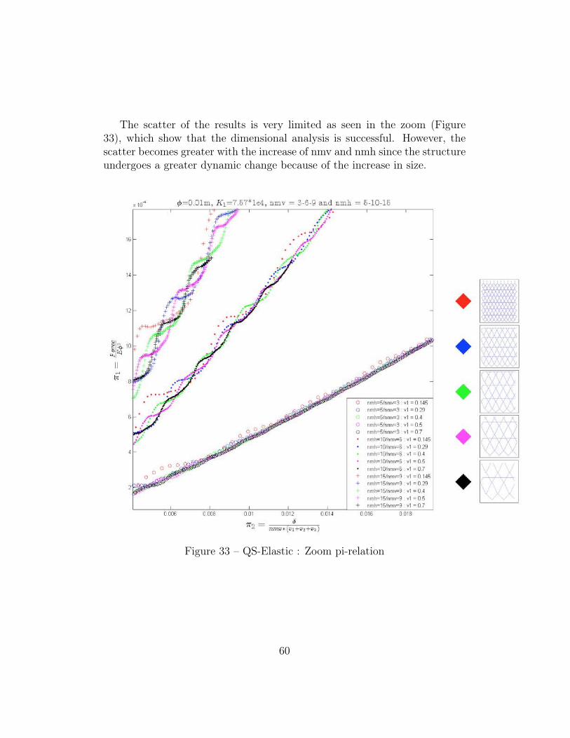
The scatter of the results is very limited as seen in the zoom (Figure33), which show that the dimensional analysis is successful. However, thescatter becomes greater with the increase of nmv and nmh since the structureundergoes a greater dynamic change because of the increase in size.
Figure 33 – QS-Elastic : Zoom pi-relation
60

The highlighted red boxes in Table 9 show the values with which theπ-terms are calculated. After changing v1, these π-terms will help find thevalues of the remaining variables.
Table 9 – Table used values QS-Elastic : Stitch
To attempt to find the solution to the problem, several different sizes ofstitch-areas were tested with a proportional maximal displacement. On theforce-displacement curve (Figure 35) it shows that all the curves have thesame shape. When placing the same values in dimensionless-form (Figure34), this results in different curves. This phenomenon has not yet beenexplained.
61

Figure 34 – QS-Elastic : Pi-relation using different sizes and displacements
62

Figure 35 – QS-Elastic : Force-Displacement using different sizes of stitch-area
4 Conclusion
The application of scaled models is of great importance in designing complexstructures because it simplifies the problem. Applying dimensional analysisto establish similarity among structural systems can save considerable time,in case the proper scaling laws are found and validated. In this study thedevelopment of similitude relations of elastic and elasto-plastic models wascarried out. The establishment of similarity conditions, based on Bucking-ham Pi-Theorem, is discussed. Numerical tests were validated by comparisonwith the theoretical results, while performing a tensile-test on the cable scaleand stitch-scale. The relations between certain π-terms show great compari-
63

son which means that the model is scale-compatible. Because of dimensionalanalysis, the number of variables are reduced to dimensionless variables whosuggest their mutual relationship. This way, the number of experiments arereduced because changes to only one parameter can result in useful informa-tion. Dimensional analysis provides us the tool to create model laws whoexpress the correlation of the behaviour between model and prototype.
5 Prospects
When following the methodology used on cable-scale, the next step will beto apply the tensile tests (in plane :Figure 36a) on stitch-scale in dynamiccondition. This will introduce new variables to consider, when applying di-mensional analysis to the structure. Afterwards, the properties of the cablestructure will receive elasto-plastic characteristics. After finishing the tensiletests IN plane, OUT of plane loading impact "punching" experiments (Fig-ure 36b) will be analysed.
(a) Tensile Test (b) Punching Test
Figure 36 – Stitch - Experiments
64
References
E. Baker, S. Westine, and F. Dodge. Similarity methods in engineering dy-
namics - Theory and pratice of scale modeling. Elsevier, 1991.
T. Szirtes. Applied dimensional analysis and modeling. Elsevier, 2007.
A. Volkwein. Numerical simulation of flexible rockfall protection systems. InProceedings of the 2005 ASCE International Conference on Computing in
Civil Engineering, 2005a.
Norman Jones. On the mass impact loading of ductile plates. Defence Science
Journal, 53(1):15, 2003.
S. Balawi, O. Shahid, and M.AlMulla. Similitude and scaling laws - static anddynamic behaviour beams and plates. Procedia Engineering, 114:330–337,2015.
Olivier Buzzi, E. Leonarduzzi, B. Krummenacher, A. Volkwein, and A. Gi-acomini. Performance of high strength rock fall meshes: Effect of blocksize and mesh geometry. Rock Mechanics and Rock Engineering, 48(3):1221–1231, 2014. ISSN 1434-453X. doi: 10.1007/s00603-014-0640-7. URLhttp://dx.doi.org/10.1007/s00603-014-0640-7.
Bernhard Pichler, Ch Hellmich, and Herbert A Mang. Impact of rocks ontogravel design and evaluation of experiments. International Journal of Im-
pact Engineering, 31(5):559–578, 2005.
A. Vaschy. Sur les lois de similitude en physique. Annales Tél’egraphiques,19:25–28, 1892.
E. Buckingham. On physically similar systems: illustrations of the use ofdimensional equations. Physical Reviews, (4)4:345, 1914.
A. Sonin. The physical basis of dimensional analysis. Technical report,Department of Mechanical Engineering MIT, 2001.
65