CHAPTER 8Design of Fuzzy Comparator Based

Differential Relay

8.1 Introdution

8.2 Characteristics of Differential Relay

8.3 Fuzzification of Characteristics Curve

8.4 Rule Base Design

8.4.1 Rule Base Design for Operating C urren t

8.4.2 Proportional Inference and Form ation of Rule Blocks

8.5 Neural Defuzzification

8.6 Hardware Implementation

8.7 Simulation Result

8.8 Practical Result Verification

8.9 Discussion

" From causes which appear sim ilar, we expect similar effects .This is the sum total of all

□ur experimental conclusions "

David Hume, Scottish philosopher

Enquiry Concerning Human Understanding ,1748

Chapter 8. Design of Fuzzy Comparator Based Differential Relay

8.1 IntroductionThe fuzzy sensor designed in previous chapters (Chapters 4,5,6 and 7) using different soft

computing tools like NN, fuzzy logic and GA are basically used for line system and substation

protection. This chapter is meant for only power system equipment protection like transformer, motor

and generator. A comparator based fuzzy differential relay has been considered here for designing a

fuzzy sensor, as this protection system is veiy popular in power system equipment. IDMT relay is

used for line and earth protection whereas ‘Differential Relay’ [97,99] is used for power system

equipment protection, the another part of the power system.

8.2 Characteristics of Differential RelayThe differential relay is connected in a Merz-price configuration to current transformers on

either side of the protected power system equipment [97]. The ratio of the current transformers (CT’s)

on the two sides of the power transformer are normally matched so that under normal load conditions,

the C.T secondary currents are equal and no current (No error) flows in the operating coil of the relay.

Under load, the C.T. secondary currents flow through the restraint coils of the relay, which produce a

continuous torque on the disc in the contact opening direction. On an internal fault in the power

transformer, the balance of the C.T. secondary currents is disturbed and the resultant differential

current flows through the relay operating coil which produces a torque on the disc in the contact

closing direction. The contacts close when the ratio of the differential current to the through current

exceeds the slope of the relay operating characteristic determined by the turns ratio of the operating

and restraint coils. A DDT 12/32 type percentage biased differential relay [97,99], manufactured by

GEC Alsthom India is considered for this research. The relay is used for biased differential protection

of two winding power transformers against internal phase and earth faults. Fig. 8.1 shows a schematic

arrangement of merz-price biased differential protection .

Fig. 8.1 Merz - price biased differential protection

Biased [97] relay has restraining winding to provide stability on external fault. Percentage bias

setting provided in this relay varies from 5 to 50% and relay current setting varies from 10 to 100% of

fault load. Both electromagnetic and static type of comparators are used. In both case we may define:

Io = operating current = I1-I2

- \ I x + h

Or

Where

Ir = restraining current =

In an electromagnetic comparator the relay will operate i f :

Operating torque >= Restraining torque +Spring torque

Ki (No Io) 2 >= K2 (N, Ir)2 +kj ...(8.1)

No = Operating turns, ki, k2 = Design constant

Nr = Restraining turns, ks = Spring torque.

At balance i.e. when the relay is just on the verge of operation, the operating torque would be

equal to spring torque (k ’sj.

Ks=K, (N o Io mi„)2 . . . ( 8 . 2 )

Io min “ pick up current of relay.

From equation 8.1 and equation 8.2 we can obtain:

K, (N„ I„) 2=K2 (N, Ir) 2+K, (No I0 „/„)2 ...(8.3)

Or

Or

Or

I02 =k2/ki ^*/T+i20 m in

K NIo2 = Kr2 Ir2 + Io2mi„ where Kr = ' 2 r

K , N ,

Io /Io min ̂̂ 0 mir/^r) 1 ...(8.4)

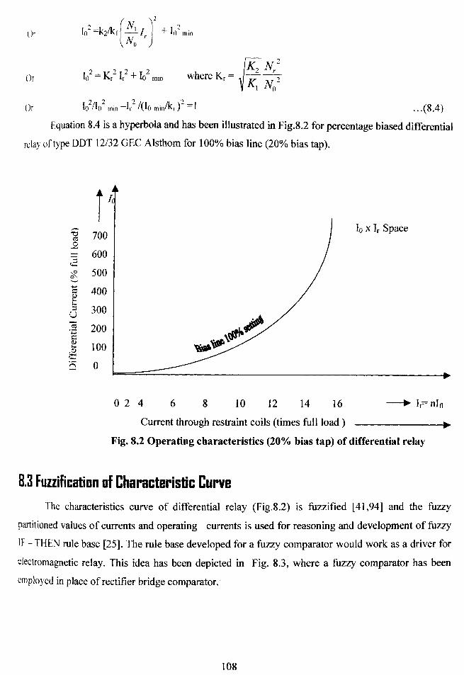
E q u a tio n 8.4 is a hyperbola and has been illustrated in Fig.8.2 for percentage biased differential

relay o f ty pe DDT 12/32 GEC Alsthom for 100% bias line (20% bias tap).

0 2 4 6 8 10 12 14 16 -----► Ir= n lfl

Current through restraint coils (times full load ) __________________^

Fig. 8.2 Operating characteristics (20% bias tap) of differential relay

8.3 Fuzzification of Characteristic CurveThe characteristics curve of differential relay (Fig.8.2) is fuzzified [41,94] and the fuzzy

partitioned values o f currents and operating currents is used for reasoning and development o f fuzzy

IF - THEN rule base [25]. The rule base developed for a fuzzy comparator would work as a driver for

electromagnetic relay. This idea has been depicted in Fig. 8.3, where a fuzzy comparator has been

employed in place of rectifier bridge comparator.

Differential Relay / \ Fuzzy

^ > 4 / I, hComparator

- ■- -»

-------► ir /A

Fig. 8.3 Fuzzy comparator for differential relay

Fig. 8.4 The three dimensional view of pyramid for fuzzy membership generation of differential relay

When there are N crisp points describing the relationship of interest (relationship between Ir

and I0), point membership function development can be repeated for each point on the product space.

This represents an exhaustive solution scheme by which all points would have a mapping rule.

From Fig 8.4, considering the “ji X Ir “ and “n X Io space ”, the salient edges facing these

planes would provide the triangular shaped membership function of restraining currents and operating

currents in Fig. 8.6 and in Fig. 8.7 respectively. Fig. 8.6 depicts the fuzzification of input variable

(Restraining current). Here the shape of membership is triangular, accept for very small (VS) and very

high (VH) linguistic predicates, for VS and VH s-shape of membership is considered in order to get

smooth characteristics curve of differential relay after simulation.

Fig. 8.5 Fuzzification of characteristics curve of differential relay shown in Fig. 8.2

Fig. 8.7 is the fuzzification of operating current obtained from the Fig. 8.5 after mapping the

input space into output space. Very small, small and slightly small membership of operating current

for its corresponding membership of restraining current are closer, that is why these all are combined

together to form a membership ‘small’ for operating current as shown in Fig. 8.7.

sfraHng9pBrai*g-current

2 4 6 8 10 12 14 16input v a r i ^ 1testrank)(f{CTenr

Fig 8.6 fuzzification of restraining current |x x l r- space

Membership 1unc1ion pi pta* | 181

oulput variable 'Operating-current" Fig 8.7 fuzzification of operating current n x l o - space

8.4 Rule Base DesignAfter fuzzification of characteristics curve of differential relay (See Fig, 8.5), rule base can be

developed [25] by expert human reasoning to infer intelligent behavior by fuzzy relay sensor.

8.4.1 Rule Base Design for Operating CurrentThe pyramid fuzziness method is used for simplicity, Fig. 8.4 illustrates the pyramid fuzziness

method for multi-input-multi-output mapping [82]. The seven crisp points of relationships on the

appex points of pyramid imply seven mapping rules given b y -

(Ir«Pvs) ---------- ► (Io *Pvs)

(Ir*PS) ---------- ► (Io *Ps)

(Ir*PSS) ---------------- ► (Io .Pss)

(Ir*PM) ----------------► (Io*Pm)

(Ir«PsH) ----------► (Io #Psh)

(Ir«PH) ----------► (Io *Ph)

(Ir*PvH) ----------► (Io*Pvh)

Where Ir = Restraining current of relay

I0 = Operating current of relay

Pvs Ps .... Pvh are predicates defined as:

Pvs = Very small

Ps = Small ,PSS = Slightly small

PM = Medium ,PSh = Slightly high

PH= High, Pvh = Very high

Referring the equation 8.5, the following 7 rules are developed [41] for inference engine of

fuzzy relay sensor-

2. If (Restraining-current is S) then (Operating-current is S) (1) ‘T"\3. If (Restraining-current is SS] then (Operating-current is S) (1 ]4. If (Restraining-current is M) then (Operating-current is M) (1)5. If (Restraining-current is SH) then (Operating-current is SH) (1)6. If (Restraining-current is H) then (Operating-current is H) (1)7. If (Restraining-current is VH) then (Operating-current is VH) (1)

z lIfjstraininq-currew m mS —SS _M SH

Fig 8.8 MATLAB output of rule base for differential relay

The above rules for differential relay can also be written in symbolic fomi as given below -

IF Ir is very small THEN Io is very Small.

IF Ir is small THEN Io is Small.

IF Ir is slightly small THEN Io is slightly Small.

1. If (Restraining-current is W | then (Operating-current is s j |'11

IF Ir is medium THEN Io is medium.

IF Ir is slightly high THEN I0 is slightly High.

IF Ir is high THEN I0 is High.

IF Ir is very high THEN I0 is very High.

As discussed before for being the membership functions of very Small, Small and Slightly

small values of I0, very closer (See Fig. 8.7) and narrower, it may be considered as a trapezoidal

shaped membership function of small values of operating current and the rule base for this region may

be written as -

IF Ir is very small THEN Io is Small

IF Ir is small THEN Io is Small

IF Ir is slightly small THEN Io is Small

Some membership functions within close proximity to each other can be represented by one

membership function completely entailing all of them. In a case where the number of crisp data points

on the product space is equal to the number of output classes such a simplification yields

approximation of the result at a level only determined by the properties of the spepific application .

8.3.2 Proportional Inference and Formation of Rule BlacksAs a method of direct mapping, proportional fuzzy inference is used provided that the problem

of design at hand suggests:

(1) Contributions to each consequent come from one rule only.

(2) All consequent membership functions are monotonically increasing or decreasing.

It is also called monotonic reasoning, where linguistic articulation of the problem in term of

complex conditional rules is possible. In its simplest form, an output is obtained by applying the

degree - of fulfillment (DOF) level of the conditions to the decomposition of the output fuzzy set

without an implication process . One can consider following rule from the mapping rules.

Ir#Pvs --------► Io*Ps . . . (8.6)

If Ir is very small then Io is small

Fig. 8.9 (a), (b) and (c) shows rule base inference process for different restraining current. In

Fig. 8.9 (a), an input value of Ir = 6 Amp for (PVs ) very small produces a scalar output Io = 87.5 Amp

for (Ps) small over the membership function contours.In the same manner in Fig. 8.9 (b) and 8.9 (c)

operating current is 251 Amp for restraining current 10 Amp and operating current is 434 Amp for

restraining current 13 Amp respectively. There is a restriction that each consequent can not be used in

more than one rule , otherwise there has to be a mechanism to reduce multiple scalar oulput to one

answer. It is to be noted that a collection of already decomposed outputs does not constitute an

aggregation problem as defined in the fuzzy logic literature because aggregation is mainly defined in

the possibility domain between fuzzy sets. In the case of multiple scalar outputs, the fuzzy system

designer may use one of the classical expert system solutions such as the Dempster-Shafer’s rules of

evidence method .The inference mechanism includes composition operators such as max-min or max-

star, an implication process such as Mamduni or Zadeh aggregation or defuzdfi$8tkm method such as the centroid method.

Reslraining-currerrt = 6

1

2

3

4

5

6

7

1. 1

/ v ....... 1

i. _.__y (

0 16

(a)

T ......... ... " "z .a _ : ...... iM l

.Az s

700

Restraining -current = 1 0

~7r~1

16

(b)

O p e ra s b-cunrorrt * 261

/ \ _______________ 11 / \ . . 'V \ i

1 A ....... ... ......... l

s :

700

Fig. 8.9 (a),(b) Proportional Inference of rules for restraining current =6 Amp. And 10 Amp.

respectively

R estra in in g-cu rren t = I S

1

2

3

4

5

6

7

_ l1 ----------- ,_ J—------

1 1"7ST- __I

1. -J. *

O p e r a t in g - !

‘G Z ?£c).V f ■» j?> ij 3 “. m r p t l s

A .I ...........- A

16

700

( C )

Fig. 8.9 ( c ) Proportional Inference of rules for restraining current *13 Amp.

Fig. 8.10 shows the simulated characteristics curve of differential relay [41]. This curve is

analogous to the original curve of differential relay as shown in Fig. 8.2. In this curve if restraining

current increases, operating current also increases. For 0-5 Amp range of restraining current operating

current is fixed i.e 100 Amp., operating current is also fixed for restraining current more than 16 Amp.

This curve is not smooth as the original one this is due to less number of rules (Only 7 rules). The

curve may be smooth by increasing the number of rules.

Fig. 8.10 Simulated characteristics curve of differential relay

There are three types of rule block architecture. The first type is the parallel architecture in

which none of the outputs affect each other. As shown in Fig. 8.11 each block receives an input set of

restraining current Ir, which may include common elements, to produce distinct outputs.

IrVSC

Input set 1

I r s c

Input set 2

IrM

Input set i

Block 1

Block 2

Block 3

IrV H

Input set NI

Block N

^ Iovs Output set 1

~^> los Output set 2

..... " losOutput set i

C > IoVH Output set N

Fig. 8.11 Parallel rule block architecture

The second type is the cascade architecture shown in Fig 8.12, in which the output from one

block becomes the input to another block . Some of the outputs from the first line of block may also be

observed at the output. This is depicted as output Iok in Fig. 8.12.

The third type is the combination of parallel and cascade structures, as shown in Fig. 8.13, here

the rule block B receives external inputs like a parallel block as well as internal inputs like a cascade

block.

One can examine the rule composition strategies. A strategy is defined as the style of approach

to problem solving that is related to the objective behind a given problem. Competitive rule formation

strategy is best understood by modeling a decision-making process similar to one in real life.

Competitive strategy employs a threshold to discriminate between the low quality and high quality

decisions .Competitive rule formation in fuzzy system design assumes that all rules in the same rule

block are intended to fire at full capacity or close to frill capacity. Weak membership functions are not

tolerated. Competitive rule formation is normally designed by applying one threshold level to the

entire rule block as depicted in Fig.8.14. Rules producing degrees of fulfillment less than the threshold

are discarded. As expected, a higher threshold produces jumpier outcome, which may be considered a

selective behavior.

IrVS

Irs

IrM

IrVH

: > Block 1

Block 2

Block 3

O Block N

Iovs-

Ios

loVH----

* 1%'S

Fig. 8.12 Cascade rule block architecture

lOC

IoK

Block A "► losi i.

■ m M c! fv-

----------- ► Block B> Iosi

----------------»

Fig 8.13 Combination of parallel and cascade arrangements of rule block architecture

As one can infer from above, threshold across all rule blocks results in selecting different

m em ber of rules from each block at a different times. However, selected rules only contribute to their

own rule block aggregation in the standard fuzzy inference algorithm.

DOF Threshold

( Ir • Pvs)

( Ir • Ps)

( Ir • Pss)

( Ir • Pm)

( Ir • PSH)

( Ir • Ph)

( Ir • PVh)

( Io • P v s )

( I o * P s)

(Io • Pss)

(I® • P « )

(Io • P vjf)

h.anip

Fig. 8.14 Competitive rule formation using block threshold

8.5 Neural DefuzzificationIt is emphasized that the connection between the discrete-time neuro-ftizzy [11] systems

obtained by combining fuzzy systems and neural network, and some classes of usual discrete systems.

The nonlinear combines are described by equations such as -

p / \ ?Ion ^ j f k {akK(n-k) ) ...(8.7)

Io„ = Operating current of nth term, I^n-k), Ir(n-i)= Restraining current of (n-k)th and (n-i)* term

ak, bj = Weight values or membership functions

Here fk and gj may be power function or polynomial functions. The equation 8.7 may also be written

as:

Ion = f\k=0 V '=1

...(8.8)

The equation 8.8 is the equation of a two - neuron (recurrent) network. The equation for single

neuron will be -

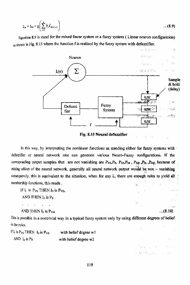
I0n = Ion + g(A )̂^0(w-0

V'=l...(8.9)

Equation 8.9 is stand for the mixed linear system or a fuzzy system ( Linear neuron configuration)

as shown in Fig. 8.15 where the function f is realized by the fuzzy system with defuzzifier.

Neuron

Fig. 8.15 Neural defuzzifler

In this way, by interpreting the nonlinear functions as standing either for fuzzy systems with

defuzzifier or neural network one can generate various Neuro-Fuzzy configurations. If the

corresponding output samples that are not vanishing are Pvs,Ps, Pss,Pm , Psh >Ph JRvh, because of

mixing effect of the neural network, generally all neural network output would be non - vanishing

consequently, this is equivalent to the situation, when for any Ir, there are enough rules to yield all

membership functions, this reads .

IF Ir is Pvs THEN Io is Pvs,AND THEN Io is Ps

AND THEN I0 is PVH •••(8.10)

This is possible in a nontrivial way in a typical fuzzy system only by using different degrees of belief in the rules.

Iflr is Pvs THEN IoisPvs with belief degree wl

AND I0 is Ps with belief degree w2

AND Io is Pss with belief degree w3

AND Io is P v h with belief degree w7 ...(8.11)

A fuzzy system with belief degrees in the rules (weighted rules) is implemented by a

simple fuzzy system followed by a neural network. The neural network is easily trimmed to determine

the belief degrees for a specific application. The above property also shows the equivalence between

the chaotic fuzzy systems with belief degree in the rules and the chaotic neuro-fuzzy systems

involving fuzzy systems with complete belief in the rules .

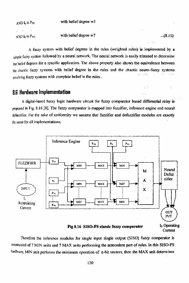
8.6 Hardware ImplementationA digital-based fuzzy logic hardware circuit for fuzzy comparator based differential relay is

proposed in Fig. 8.16 [8]. The fuzzy comparator is mapped into fuzzifier, inference engine and neural

defuzzifier. For the sake of uniformity we assume that fuzzifier and defuzzifier modules are exactly

the same for all implementations.

Fig 8.16 SISO-FS classic fuzzy comparator Io OperatingCurrent

Therefore the inference modules for single input single output (SISO) fuzzy comparator is

constructed of 7 MIN units and 7 MAX units performing the antecedent part of rules. In this SISO-FS

hardware, MIN unit performs the minimum operation of n-bit vectors, then the MAX unit determines

the maximum values represented by one of these n-bit vectors . The antecedent (Ir) membership

functions are stored and made ready to enter the MIN units. These functions are stored in the rule base

memory proceeding with fuzzy inference, the consequent (I0) membership functions are entered into

7 MIN units. The results of consequent MIN units are united by means of a multi-input MAX unit.

Finally the unified neural defuzzifier generates a crisp output of fuzzy comparator.

8.7 Simulation ResultsAntecedent variables (Restraining current) are considered numerically for different

membership function from Fig. 8.6 as given below -

( 1 , 2 , 3, 4.5, 5.5 , 6 7 , 8 . 5 , 10 , 1 0 . 5 , 12 , 1 3 . 5 , 1 4 . 5 , 1 6 ) ...(8.12)

< -VS— >< —S— > <---- SS.......>< —M— >< —SH— > < —H— > <r------- VH----->

corresponding consequent variables (Operating current) are considered numerically for

different membership function from Fig. 8.7 as given below -

( 50,60,75,100,125,160, 175, 240,275, 300,350, 400,460,575) ...(8.13)

<-........... S-------------> < —M------ >< —SH------ >< —H— > < ----- VH— >

The antecedent variables and consequent variables obtained and written in equation 8.12 and

8.13 from the design data referring Fig. 8.6 and Fig. 8.7 respectively can be written in zadeh’s

notation as given below -

0.95 0.36 0.66 0.33 1 0.66 0.66 0.33 0.66 0.33 0.66 0.31 0.97 O----- 1------- 1--------1--------1------ 1--------1--------1--------1--------1-------- 1-------- 1----- - H--------1----1 2 3 4.5 5.5 6 7 8.5 10 10.5 12 13.5 14.5 16

Io = -L+-L J_ J_ 9̂ 1 91. 911 9* 9* 91_ 91_ 9J1 0̂ 2 05450 60 + 75 + 100 + 125 + 160 + 175 + 240 + 275 + 300 + 350 + 400 + 460 575

Table 8.1 shows the designed and simulated value of antecedent and consequent variable of

differential relay. Simulated values are obtained for various values of ‘n’ from manufacturer designed data.

For the design values of Ir and Io, the simulation results are shown in the Table 8.1 with their

membership functions. The designed and simulated values are very much compromising and the errors

are within the prescribed limit. The simulator circuit thus obtained would be capable to perform the

duties of differential relay, as the simulator is based on the characteristic curve of differential relay.

The fault current of either crisp or fuzzy value would capture the rules from Rule-base and aggregate

the results to provide fuzzy value of operating current which can further be defuzzified to obtain an

action current.

Table 8.1- Design and Simulated antecedent and consequent variables and its membership of

differential Relay

s

No

Antecedent Variables (Restraining Current Ir) Consequent Variables (Operating Current

Io)Designed

Values

Simulated values Error

in

Ir

Designed

Values

Simulated

values

Error

in

IoIr=

nlfiM- (ir) Ir=nlfl M- (Ir) Io M- (io) Io M'(io)

1 1 0.95 0.98792 0.949 0.01208 50 1 49.990 0.998 0.010

2 2 0.36 2.03002 0.365 -0.03002 60 1 59.987 0.998 0.013

3 3 0.66 3.03220 0.668 -03220 75 1 74.970 0.997 0.030

4 4.5 0.33 4.50200 0.335 -0.00200 100 1 99.998 0.998 0.002

5 5.5 1 5.49040 0.998 0.0096 125 0.95 125.092 0.953 -0.092

6 6 0.66 5.99988 0.659 0.00012 160 0.3 160.012 0.320 -0.012

7 7 0.66 6.89988 0.659 0.10012 175 0.55 175.120 0.552 -0.120

8 8.5 0.33 8.50073 0.337 -0.00073 240 0.8 239.987 0.798 0.013

9 10 0.66 10.0001 0.666 - 0 . 0 0 0 1 275 0.8 274.899 0.798 0.101

10 10.5 0.33 10.4998 0.329 0.0002 300 0.5 300.032 0.502 -0.032

11 12 0.66 11.5331 0.658 0.4669 350 0.5 349.998 0.497 0.002

12 13.5 0.31 13.500121 0.318 -0.00012 400 0.75 400.207 0.758 -0.207

13 14.5 0.97 14.499099 0.968 0.00090 460 0.72 459.998 0.719 0.002

14 16 1 15.99009 0.999 0.00991 575 0.54 575.020 0.542 -0.020

8.8 Practical Result VerificationThe power transformer 3, 33KV/11KV, 20 MVA in KORBA city east substation was

considered for testing the simulation .The operating coil current in normal operating condition was

found to be zero, an artificial fault in the form of short circuit, open circuit and earth fault was

developed .The readings are being presented in tabular form (Table 8.2 ). The differential relay also

operates for the excessive overloading. The performance of conventional differential relay and the

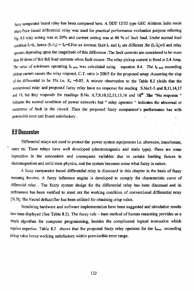
fuzzy comparator based relay has been compared here. A DDT 12/32 type GEC Alsthom India made

M erz-P rice biased differential relay was used for practical performance evaluation purpose referring

Fig. 8.1 relay setting was at 20% and current setting was at 40 % of fault load. Under normal load

condition I)=l2, hence (I1-I2) = Io=O.For an internal fault Ij and I2 are different .So (Ii-^^O and relay

operates depending upon the magnitude of this difference .The fault currents are considered to be more

than 10 times of this full load currents when fault occurs .The relay pickup current is fixed at 0.4 Amp.

The value of minimum operating Io min was calculated using equation 8.4. The Io min exceeding

pickup current causes the relay respond, C.T. ratio is 200/5 for the proposed setup .Assuming the slop

of the differential to be 5% i.e. Kr =0.05. A minute observation to the Table 8.2 yields that the

conventional relay and proposed fuzzy relay have no response for reading S.No.1-5 and 8,11,14,17

and 19, but they responds for readings S.No. 6,7,9,10,12,13,15,16 and 18* .The “No response “

indicates the normal condition of power networks but “ relay operates “ indicates tile abnormal or

occurrence of fault in the circuit .Thus the proposed fuzzy comparator’s performance has with

permissible error and found satisfactory .

8.9 DiscussionDifferential relays are used to protect the power system equipments i.e. alternator, transformer,

1 motor etc. These relays have well developed (electromagnetic and static type). There are some

imprecision in the antecedent and consequent variables due to certain limiting factors in

electromagnetism and solid state physics, and the system becomes some what fuzzy in nature.

A fuzzy comparator based differential relay is discussed in this chapter in the basis of fuzzy

reasoning theories. A fuzzy inference engine is developed to comply the characteristic curve of

differential relay . The fuzzy system design for the differential relay has been discussed and its

performance has been verified to meet out the working condition of conventional differential relay

[76,78]. The Neural defuzzifier has been utilized for obtaining crisp value.

Simulating hardware and software implementation have been suggested and simulation results

have been displayed (See Table 8.2). The fuzzy rule - base method of human reasoning provides us a

simple algorithm for computer programming, besides the complicated logical instruction which

requires expertise. Table 8.2 shows that the proposed fuzzy relay operates for the Iomin exceeding

pickup value hence working satisfactory within permissible error range.

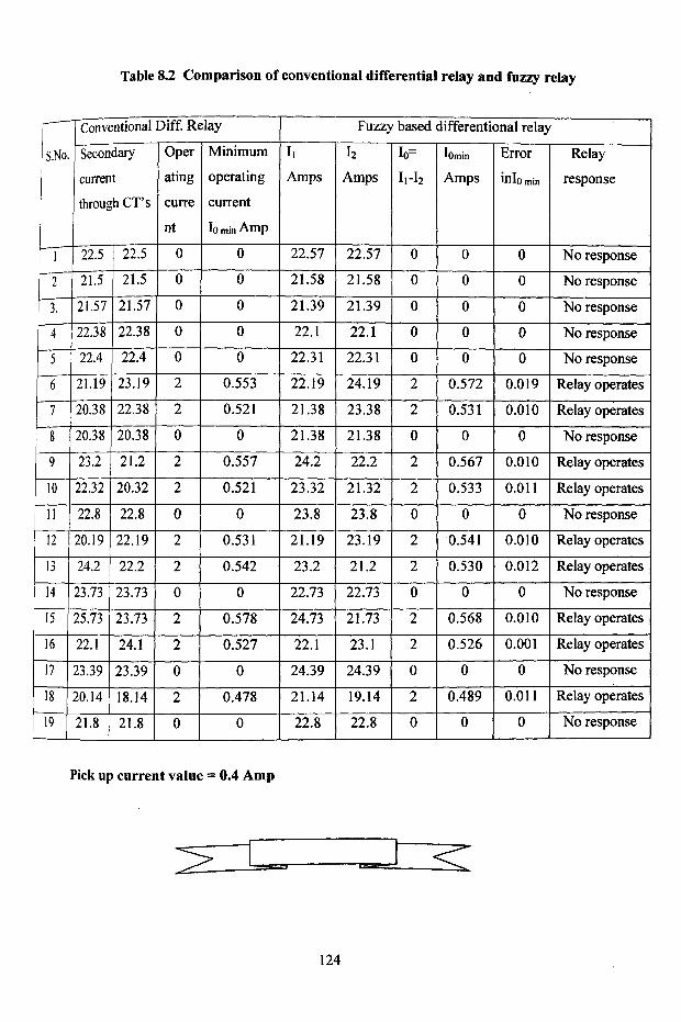
Table 8.2 Comparison of conventional differential relay and fuzzy relay

S.No.

Conventional Diff. Relay Fuzzy based differentional relay

Secondary

current

through CT’s

Oper

ating

curre

nt

Minimum

operating

current

Io min Amp

Ii

Amps12

AmpsIo=

I1-I2

lomin

Amps

Error

inlo min

Relay

response

1 22.5 22.5 0 0 22.57 22.57 0 0 0 No response

2 21.5 21.5 0 0 21.58 21.58 0 0 0 No response

3. 21.57 21.57 0 0 21.39 21.39 0 0 0 No response

4 22.38 22.38 0 0 22.1 22.1 0 0 0 No response

5 22.4 22.4 0 0 22.31 22.31 0 0 0 No response

6 21.19 23.19 2 0.553 22.19 24.19 2 0.572 0.019 Relay operates

7 20.38 22.38 2 0.521 21.38 23.38 2 0.531 0.010 Relay operates

8 20.38 20.38 0 0 21.38 21.38 0 0 0 No response

9 23.2 21.2 2 0.557 24.2 22.2 2 0.567 0.010 Relay operates

10 22.32 20.32 2 0.521 23.32 21.32 2 0.533 0.011 Relay operates

11 22.8 22.8 0 0 23.8 23.8 0 0 0 No response

12 20.19 22.19 2 0.531 21.19 23.19 2 0.541 0.010 Relay operates

13 24.2 22.2 2 0.542 23.2 21.2 2 0.530 0.012 Relay operates

14 23.73 23.73 0 0 22.73 22.73 0 0 0 No response

15 25.73 23.73 2 0.578 24.73 21.73 2 0.568 0.010 Relay operates

16 22.1 24.1 2 0.527 22.1 23.1 2 0.526 0.001 Relay operates

17 23.39 23.39 0 0 24.39 24.39 0 0 0 No response

18 20.14 18.14 2 0.478 21.14 19.14 2 0.489 0.011 Relay operates

19 21.8 21.8 0 0 22.8 22.8 0 0 0 No response

Pick up current value = 0.4 Amp