Design of Fractional-Order PIa Controller For Integer

International Journal of Scientific & Engineering Research, Volume 4, Issue 5, May-2013 743 ISSN 2229-5518

IJSER © 2013

http://www.ijser.org

Design of Fractional-Order PIα Controller For Integer-Order Systems

Adil Zulfiqar, Nisar Ahmed

Abstract—The aim of this work is to design a fractional-Order PIα controller for Integer-order type systems so that to improve the performance and robustness of integer-order type systems. The design of FO-PIα controller in the sense that good set-point tracking and load disturbance rejection is minimized by increasing fractional-order element “α” putting constraint on peak sensitivity function. The method used in this paper is generalized method i.e. Fractional-Ms Constrained integral gain optimization (F-MIGO). In this method it is assumed that model of the plant is given to us. The method is very effective and simple to use. At the end comparison between fractional PIα and classical PI controllers is give.

Index Terms—Fractional order Calculus; Integer order systems; constraint optimization; robust controller design

—————————— ——————————

1 INTRODUCTION The Classical PID (Proportional+Integral+Derivative)

controllers are dominated the industry because of their performance, robustness to system’s variations, simplicity and available of different kinds of tuning rules [1]. Now-a-days 90% of industrial closed loops contain PID/PI controllers [2,3]. In the field of dynamic research improvement in the performance is the primary concern.

In the last few years Fractional Calculus (FC) opened the doors for research [4,5,6] and its applications in the field of control systems [7,8]. Fractional calculus became very hot topic in these years in the field of control [9,10,11,12] for fractional order controller design for integer order systems as well as for fractional order systems [13]. Fractional Calculus provides us powerful tool for memory and hereditary effects in various materials [14].

Clearly, in closed loop control systems we have four combinations: (1) integer-order (IO) controllers for integer-order (IO) systems; (2) integer-order (IO) controllers for fractional-order (FO) systems; (3) fractional-order (FO) controllers for integer-order (IO) systems; (4) fractional-order (FO) controllers for fractional-order (FO) systems. In this paper fractional order proportional integral controller is designed for integer order systems to improve the performance and robustness of integer order systems. The method used in this paper to design fractional order proportional integral controller is the generalized form of MIGO which is used in [15,16].

As shown in [15,16] that increase fractional order “α” putting constraint on peak sensitivity function “Ms” load disturbance rejection can be minimized. The assumption of this method is that the model of the plant is already provided to us. By using the same method an

integer order proportional integral order (IOPI) can be designed. At the end comparison between fractional order proportional integral controller (FOPI) and integer order proportional integral controller (IOPI) is also made.

The rest of this paper is organized as follows. In section II, the introduction of fractional calculus is given. In section III, the design goal and problem is formulated. In section IV, the design procedure is considered. In section V, the simulation results and comparison is established. Conclusion and future work is given in section VI, and at the end references will close the paper.

2 INTRODUCTION OF FRACTIONAL CALCULUS The origin of fractional calculus is old as classical calculus. The history of fractional calculus began at the end of 17th century with the exchange of letters between two most prominent mathematicians at that time i.e. Leibniz and L’Hobital. In particular, in one of those letters, Leibniz wrote a letter to L’Hobital that and asked a question [17] “Can the integer order be generalized to non-integer orders”. L’Hobital became very surprised and replied with another question “What if the order will be 1/2?. Leibniz replied in a letter dated 30th September 1695 wrote the very famous words that “One day it will led to paradox from which useful results can be drawn”.

Now-a-days, on the basis of those letters many mathematicians and researchers agreed that exact birth of fractional calculus is 30th September 1695 and Gottfried Leibniz is father of fractional calculus [18]. 2.1 Definition of Fractional Calculus: The fractional-order fundamental differential arithmetic operator “ a𝐷𝑡

𝑞 “ is introduced as follows [19]:

IJSER

http://www.ijser.org/


IJSER © 2013


a𝐷𝑡𝑟 =�

𝑑𝑟

𝑑𝑡𝑟 ,𝑅𝑒(𝑟 > 0)

1 ,𝑅𝑒(𝑟 = 0)∫ (𝑑𝜏)−𝑟 ,𝑅𝑒(𝑟 < 0)𝑡𝑎

� (2.1)

Where ‘r’ is the fractional order and can be complex and real number. The constants ‘a’ and ‘t’ are initial conditions. There are commonly three definitions used for fractional differentiations and integrations i.e.

The Grunwald-Letnikov (GL) definition is given below:

a𝐷𝑡𝑟𝑓(𝑡) = limℎ ℎ−𝑟 ∑ (−1)𝑗 �𝑟𝑗� 𝑓(𝑡 − 𝑗ℎ)

[𝑡−𝑎]ℎ

𝑗=0 (2.2) Where [.] is an integer part. The Riemann-Liouville (RL) definition is given below: a𝐷𝑡𝑟𝑓(𝑡)= 1

Г(𝑛−𝑟)𝑑𝑛

𝑑𝑡𝑛∫ 𝑓(𝜏)

(𝑡−𝜏)𝑟−𝑛+1𝑑𝜏𝑡

𝑎 (2.3)

for (n-1<r<n) and where Г(.) is the Gamma function. The Caputo definition can be written as: a𝐷𝑡𝑟𝑓(𝑡) = 1

Г(𝑛−𝑟)∫ 𝑓𝑛(𝜏)

(𝑡−𝜏)𝑟−𝑛+1𝑑𝜏𝑡

𝑎 (2.4) for (n-1<r<n).

These above definitions are the key of fractional order control systems. These equations provide and awesome instruments for the description of memory and hereditary properties of many materials and process dynamics [20].

Comparison between these three fractional derivatives and integrals shows that, the improvement of Grunwald-Letnikov definition are Riemann-Liouville and Caputo definitions. The fractional derivative calculation can be simplified by using Riemann-Letnikiv definition and with the help of Caputo definintion the Laplace transform can be more summarized for the discussion of fractional differential equations.

3 THE DESIGN GOAL The design aim of this paper is that load disturbances rejection is minimized and good set-point tracking. Load disturbances and set-point signals are very low frequency signals and their attenuation is the primary task of any controller. It is shown in [21] that maximizing integral gain Ki the load disturbance at the output can be minimized. Load disturbance is defined by 𝐼𝐴𝐸 = ∫ |𝑒(𝑡)|𝑑𝑡∞

0 (3.1) 𝐼𝐸 = ∫ 𝑒(𝑡)𝑑𝑡∞

0 (3.2)

It is proved in [21] that IE= 1𝐾𝑖

, thus maximizing integral

gain reduces the effect of load disturbance at the output.

3.1 THE DESIGN PROBLEM The design problem can be stated as: “Maximize Ki to obtain parameters of Proportional Integral (PIα) so that the closed loop system if and only if nyquist curve lies outside the circle with centre at s=-C and with radius R”.

4 THE DESIGN PROCEDURE The design procedure comprises the following steps. 4.1 The design parameters: The defined loop transfer function of typical plant is P(s)=C(s)G(s), where C(s) is the controller transfer function and G(s) is the plant transfer function. Now we define two functions for load disturbance rejection and set-point tracking. 𝑆(𝑠) = 1

1+𝐶(𝑠)𝐺(𝑠) (4.1)

𝑇(𝑠) = 𝐶(𝑠)𝐺(𝑠)

1+𝐶(𝑠)𝐺(𝑠) (4.2)

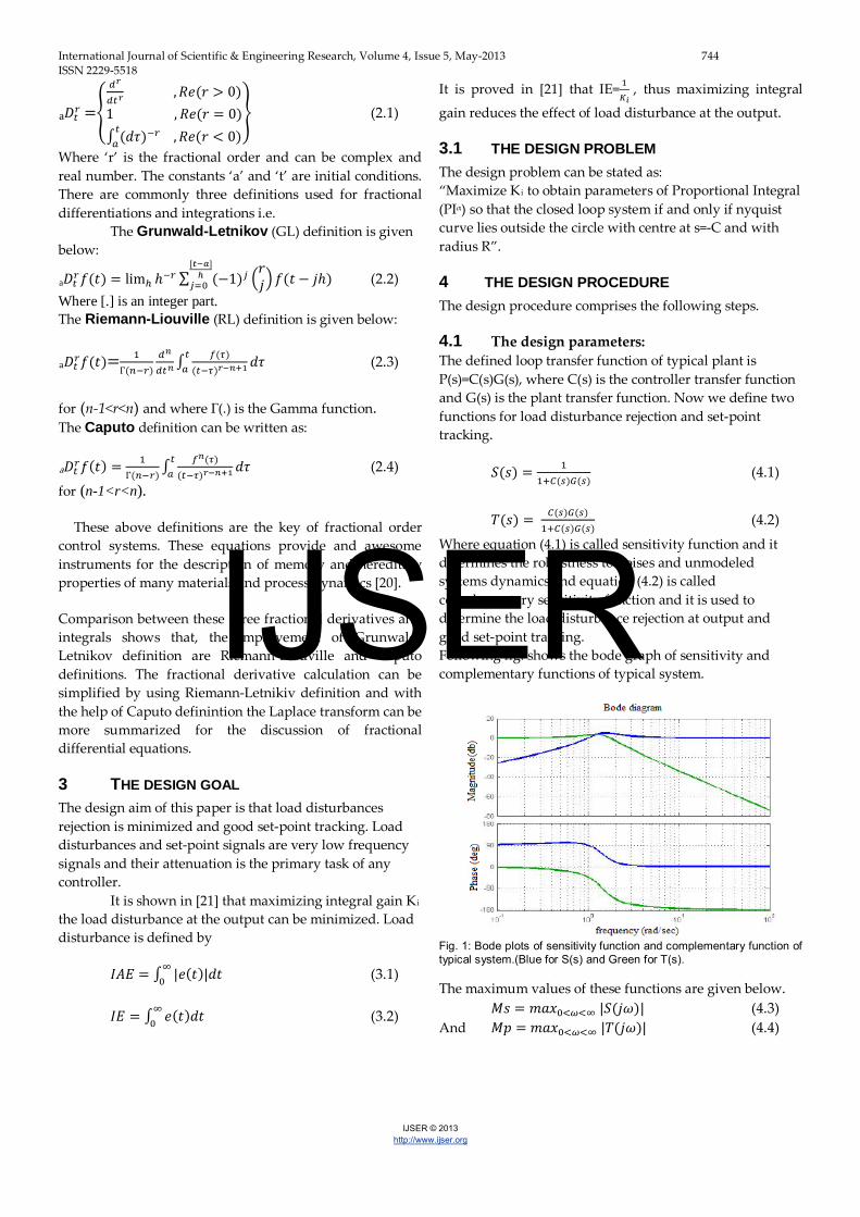
Where equation (4.1) is called sensitivity function and it determines the robustness to noises and unmodeled systems dynamics and equation (4.2) is called complementary sensitivity function and it is used to determine the load disturbance rejection at output and good set-point tracking. Following fig. shows the bode graph of sensitivity and complementary functions of typical system.

Fig. 1: Bode plots of sensitivity function and complementary function of typical system.(Blue for S(s) and Green for T(s). The maximum values of these functions are given below. 𝑀𝑠 = 𝑚𝑎𝑥0<𝜔<∞ |𝑆(𝑗𝜔)| (4.3) And 𝑀𝑝 = 𝑚𝑎𝑥0<𝜔<∞ |𝑇(𝑗𝜔)| (4.4)

IJSER



IJSER © 2013


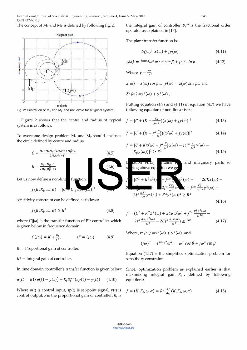
The concept of Ms and Mp is defined by following fig. 2.

Fig. 2: Illustration of Ms and Mp and unit circle for a typical system.

Figure 2 shows that the centre and radius of typical system is as follows:

To overcome design problem Ms and Mp should encloses the circle defined by centre and radius.

𝐶 = 𝑀𝑠−𝑀𝑠𝑀𝑝−2𝑀𝑠𝑀𝑝2+𝑀𝑝

2−1

2𝑀𝑠(𝑀𝑝2−1)

(4.5)

𝑅 = 𝑀𝑠−𝑀𝑝−1

2𝑀𝑠(𝑀𝑝2−1)

(4.6)

Let us now define a non-linear function:

𝑓(𝐾,𝐾𝑖 , ,𝜔,𝛼) = |𝐶 + 𝐶(𝑗𝜔)𝐺(𝑗𝜔)|2 P

(4.7)

sensitivity constraint can be defined as follows:

𝑓(𝐾,𝐾𝑖 , ,𝜔,𝛼) ≥ 𝑅2 (4.8)

where C(j𝜔) is the transfer function of PIα controller which is given below in frequency domain:

𝐶(𝑗𝜔) = 𝐾 + 𝐾𝑖𝑆𝛼

, 𝑠𝛼 = (𝑗𝜔) (4.9)

𝐾 = Proportional gain of controller.

𝐾𝑖 = Integral gain of controller.

In time domain controller’s transfer function is given below:

𝑢(𝑡) = 𝐾�𝑠𝑝(𝑡) − 𝑦(𝑡)� +𝐾𝑖𝐷𝑡−𝛼(𝑠𝑝(𝑡)− 𝑦(𝑡)) (4.10)

Where u(t) is control input, sp(t) is set-point signal, y(t) is control output, 𝐾is the proportional gain of controller, 𝐾𝑖 is

the integral gain of controller, 𝐷𝑡−𝛼 is the fractional order operator as explained in [17].

The plant transfer function is:

G(j𝜔)=𝑥(𝜔) + 𝑗𝑦(𝜔) (4.11)

(j𝜔)α=𝑒𝑗𝜋𝛼/2𝜔𝛼= 𝜔𝛼 𝑐𝑜𝑠 𝛽 + 𝑗𝜔𝛼 𝑠𝑖𝑛 𝛽 (4.12)

Where 𝛾 = 𝜋𝛼2

,

𝑥(𝜔) = 𝑧(𝜔) 𝑐𝑜𝑠𝜑 𝜔, 𝑦(𝜔) = 𝑧(𝜔) 𝑠𝑖𝑛 𝜑𝜔 and

𝑍2(𝜔) =𝑥2(𝜔) + 𝑦2(𝜔) ,

Putting equation (4.9) and (4.11) in equation (4.7) we have following equation of non-linear type.

𝑓 = |𝐶 + (𝐾 + 𝐾𝑖(𝑗𝜔)𝛼)(𝑥(𝜔) + 𝑗𝑦(𝜔)|2 (4.13)

𝑓 = |𝐶 + (𝐾 − 𝑗𝛼 𝐾𝑖𝜔𝛼)(𝑥(𝜔) + 𝑗𝑦(𝜔)|2 (4.14)

𝑓 = |𝐶 +𝐾𝑥(𝜔) − 𝑗𝛼 𝐾𝑖𝜔𝛼 𝑥(𝜔) − 𝑗(𝑗𝛼 𝐾𝑖

𝜔𝛼 𝑦(𝜔) − 𝐾𝑝𝑦(𝜔))|2 ≥ 𝑅2 (4.15)

Equation (4.15) contains real and imaginary parts so solving above equation we get:

𝑓 = |𝐶2 +𝐾2𝑥2(𝜔) + 𝑗2𝛼 𝐾𝑖2

𝜔2𝜔 𝑥2(𝜔) + 2𝐶𝐾𝑥(𝜔) −

2𝐶𝑗𝛼 𝐾𝑖𝜔𝛼 𝑥(𝜔) − 2𝑗𝛼 𝐾𝐾𝑖

𝜔𝛼 𝑥2(𝜔) + 𝑗2𝛼 𝐾𝑖2

𝜔2𝜔 𝑦2(𝜔)−

2𝑗𝛼 𝐾𝐾𝑖𝜔𝛼 𝑦2(𝜔) +𝐾2𝑦2(𝜔)|2 ≥ 𝑅2

(4.16)

𝑓 = (𝐶2 +𝐾2𝑍2(𝜔) + 2𝐶𝐾𝑥(𝜔) + 𝑗2𝛼 𝐾𝑖2𝑍2(𝜔)

𝜔2𝛼 −

2𝑗𝛼 𝐾𝐾𝑖𝑍2(𝜔)𝜔𝛼 − 2𝐶𝑗𝛼 𝐾𝑖𝑥(𝜔)

𝜔𝛼 ) ≥ 𝑅2 (4.17)

Where, 𝑧2(𝜔) =𝑥2(𝜔) + 𝑦2(𝜔) and

(𝑗𝜔)𝛼 = 𝑒𝑗𝜋𝛼/2𝜔𝛼 = 𝜔𝛼 𝑐𝑜𝑠 𝛽 + 𝑗𝜔𝛼 𝑠𝑖𝑛 𝛽

Equation (4.17) is the simplified optimization problem for sensitivity constraint.

Since, optimization problem as explained earlier is that maximizing integral gain 𝐾𝑖 , defined by following equations:

𝑓 = (𝐾,𝐾𝑖 ,𝜔,𝛼) = 𝑅2, 𝜕𝑓𝜕𝜔

(𝐾,𝐾𝑖 ,𝜔,𝛼) (4.18)

IJSER



IJSER © 2013


The above equation (4.18) shows that the derivative of function 𝑓 with respect to frequency is zero i.e. in the case of continuous derivative we have following equations.

𝑑𝑓 = 𝜕𝑓𝜕𝐾𝑑𝐾 + 𝜕𝑓

𝜕𝐾𝑖𝑑𝐾𝑖 + 𝜕𝑓

𝜕𝜔𝑑𝜔 = 0 (4.19)

In this case fractional order α is kept constant. From equation (4.19) we observe following results:

1. From (4.18) we have 𝜕𝑓𝜕𝜔

= 0.

2. For maximum 𝐾𝑖 ,𝑑𝐾𝑖 = 0.

3. And also for random variations 𝜕𝑓𝜕𝐾

= 0.

Hence for the above explained conditions the maximum of 𝐾𝑖 occur at the point of continuous derivative which is given below:

𝑓 = (𝐾,𝐾𝑖 ,𝜔,𝛼) = 𝑅2, 𝜕𝑓𝜕𝜔

(𝐾,𝐾𝑖 ,𝜔,𝛼) = 0. 𝜕𝑓𝜕𝐾

(𝐾,𝐾𝑖 ,𝜔,𝛼) = 0. (4.20)

The above three equations are non-linear and the solution of these non-linear equations can be found by the method so called Newton-Raphson as explained in [21].

From equation (4.17) we have

𝑓 = (𝐶2 +𝐾2𝑍2(𝜔) + 2𝐶𝐾𝑥(𝜔) + 𝑗2𝛼 𝐾𝑖2𝑍2(𝜔)

𝜔2𝛼 −

2𝑗𝛼 𝐾𝐾𝑖𝑍2(𝜔)𝜔𝛼 − 2𝐶𝑗𝛼 𝐾𝑖𝑥(𝜔)

𝜔𝛼 ) = 𝑅2 (4.21)

Putting (𝑗𝜔)𝛼 = 𝑒𝑗𝜋𝛼/2𝜔𝛼 = 𝜔𝛼 𝑐𝑜𝑠 𝛽 + 𝑗𝜔𝛼 𝑠𝑖𝑛 𝛽

In (4.21) we have

𝑓 =(𝐶2 + 𝐾2𝑧2(𝜔) + 2𝐶𝐾𝑥(𝜔) + 𝐾𝑖

2𝑍2(𝜔)

𝜔2𝛼 + 2𝐾𝐾𝑖𝑍2(𝜔)𝑐𝑜𝑠 𝛽𝜔𝛼 +

2𝐶𝐾𝑖(𝑥(𝜔) 𝑐𝑜𝑠𝛽+𝑦(𝜔) 𝑠𝑖𝑛𝛽)𝜔𝛼 ) = 𝑅2 (4.22)

𝜕𝑓𝜕𝜔

=

2𝐾𝑟𝑟` + 2𝐶𝐾𝑎𝑥` +𝐾𝑖2 �𝑧2

𝜔2𝛼�`

+ 2𝐾𝐾𝑖 𝑐𝑜𝑠 𝛽 �𝑍2

𝜔𝛼�`+

2𝐶𝐾𝑖 �𝑥𝜔𝛼�

`𝑐𝑜𝑠 𝛽 + 2𝐶𝐾𝑖 �

𝑦𝜔𝛼�

`𝑠𝑖𝑛 𝛽 = 0

(4.23)

𝜕𝑓𝜕𝐾

= 2𝐾𝑍2 + 2𝐶𝑥(𝜔) + 2𝑍2𝐾𝑖 𝑐𝑜𝑠𝛽𝜔𝛼 = 0 (4.24)

In the above equation (4.23) (`) means derivative with respect to the frequency in radians.

Using equations (4.22-4.24) we can find controller gains which are given below.

𝐾𝑖 = − 𝑅𝜔𝛼

𝑍 𝑠𝑖𝑛𝛽− 𝐶𝑦𝜔𝛼

𝑍2 𝑠𝑖𝑛 𝛽 (4.25)

𝐾 = 𝑅 𝑐𝑜𝑠 𝛽𝑠𝑖𝑛𝛽

+ 𝐶𝑦𝑍2

𝑐𝑜𝑠 𝛽𝑠𝑖𝑛𝛽

− 𝐶𝑥𝑍2

(4.26)

Since equations (4.25), (4.26) are the solutions of controller’s gains and these are dependent on frequency “𝜔”, so we need to find this frequency. Putting equations (4.25) and (4.26) in (4.24) we get final solution for our optimization problem.

𝜕𝑓𝜕𝜔

= 2𝑅2

𝑍𝑍` + 4𝑅𝐶𝑦

𝑍2𝑍` − 2𝛼𝑅2

𝜔− 2𝛼𝑅𝐶𝑦

𝑍𝜔− 2𝑅𝐶

𝑍𝑦 ` (4.27)

Where ` shows the derivative with respect to the frequency “𝜔”. Equation (4.27) can be simplified as explained in [21] to have simplified algebraic expression given below.

𝑇(𝜔) = 𝜕𝑓𝜕𝜔

= 2𝑅 ��𝐶 𝑦𝑍

+ 𝑅� �𝑍`

𝑍− 𝛼

𝜔� − 𝐶 �𝑦

𝑍� `� (4.28)

Now we are at the position to solve equation (4.28) to find optimal value of “𝜔𝑜” at which integral gain “𝐾𝑖 ” has maximum value, and after that we can compute values of controller’s gains 𝐾𝑖 ,𝑎𝑛𝑑 𝐾 by using equations (4.25) and (4.26) respectively.

Hence, now we apply this procedure on the test batch, so that we can conclude that fractional order controllers are superior to the integer order controllers.

4.2 Test Batch: The test batch is used so that the developed method is applied and conclude the results and check the validity of developed procedure. First of all choice for the test batch was the set of systems given in [22]. However, most of the systems can be approximated by the fractional order plus delay time (FOPDT) model, whose structure is given below: 𝐺(𝑠) = 𝑘 𝑒−𝐿𝑠

𝑇𝑠+1 (4.29)

Where 𝑘 is process gain which is assumed to be unity for all systems; L and T are delay and time constant of the system, respectively. The FOPDT models are qualify by a very important parameter which is relative dead time of the system which is given below:

IJSER



IJSER © 2013


𝜏 = 𝐿𝐿+𝑇

(4.30) Where parameter 𝜏 ranges from 0 to 1. There are two type of systems here that depends upon on𝐿 and 𝑇i.e. “Delay Dominated” and “Lag Dominated” if 𝐿 ≫ 𝑇 then it is delay dominated and if 𝑇 ≫ 𝐿 then it is termed as lag dominated.

5 SIMULATION AND COMPARISON In this section, we took some process and applied this method on these systems and show their results. Some systems are listed below:

𝐺1(𝑠) =1

0.05𝑠 + 1𝑒−𝑠 , 𝐺2(𝑠) =

1(𝑠 + 1)3 𝑒

−15𝑠

𝐺3(𝑠) =1

(1 + 𝑠)(1 + 0.2𝑠)(1 + 0.04𝑠)(1 + .008𝑠)

𝐺4(𝑠) = 1(𝑠+1)(0.2𝑠+1)

Thus from the above four systems we have 2 delay dominated systems 𝐺1(𝑠) and 𝐺2(𝑠) , and two lag dominated systems 𝐺3(𝑠) and 𝐺4(𝑠).

TABLE 1

FOPDT parameters for systems 𝐺1(𝑠) to 𝐺4(𝑠)

System 𝑘 𝐿 𝑇 𝜏 Type

𝐺1(𝑠) 1 1 0.09 0.92 Delay Dominant

𝐺2(𝑠) 1 16.23 1.76 0.9 Delay Dominant

𝐺3(𝑠) 1 0.1436 2.65 0.051 Lag Dominant

𝐺4(𝑠) 1 0.105 1.11 0.09 Lag Dominant

Following table shows the controller parameters for the above four systems. In this table controller’s gains and Integral Squared Error (ISE) and maximum sensitivity is given using F-MIGO algorithm and compare it with other tuning rules.

TABLE 2

Parameters of controller for given systems

𝐺1(𝑠) 𝐺2(𝑠)

Method 𝛼 𝐾 𝐾𝑖 𝑀𝑠 ISE 𝐾 𝐾𝑖 𝑀𝑠 ISE

FMIGO

1.1 .32 .53 1.4 1.32 .33 .03 1.4 20.8

NZ 1 .41 .24 1.7 2 .42 .014 1.7 32.3

𝐺3(𝑠) 𝐺4(𝑠)

Method 𝛼 𝐾 𝐾𝑖 𝑀𝑠 ISE 𝐾 𝐾𝑖 𝑀𝑠 ISE

FMIGO .7 5.8 5.7 1.4 .29 3.4 7.6 1.4 .2

NZ 1 11.8 26.3 2.4 .3 6.9 21.3 2.3 .2

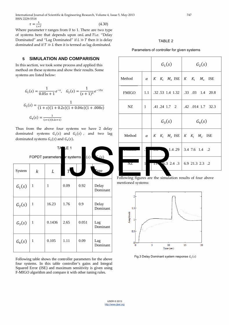
Following figures are the simulation results of four above mentioned systems:

Fig.3 Delay Dominant system response 𝐺1(𝑠)

IJSER



IJSER © 2013


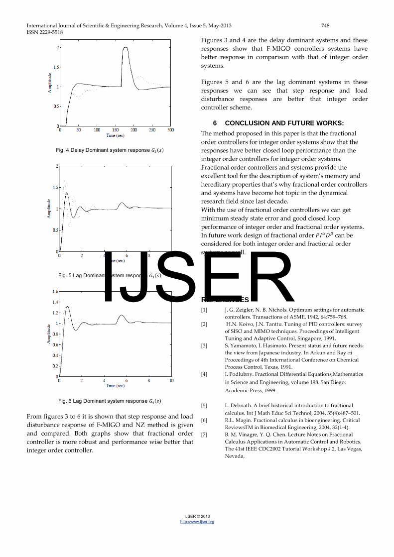
Fig. 4 Delay Dominant system response 𝐺2(𝑠)

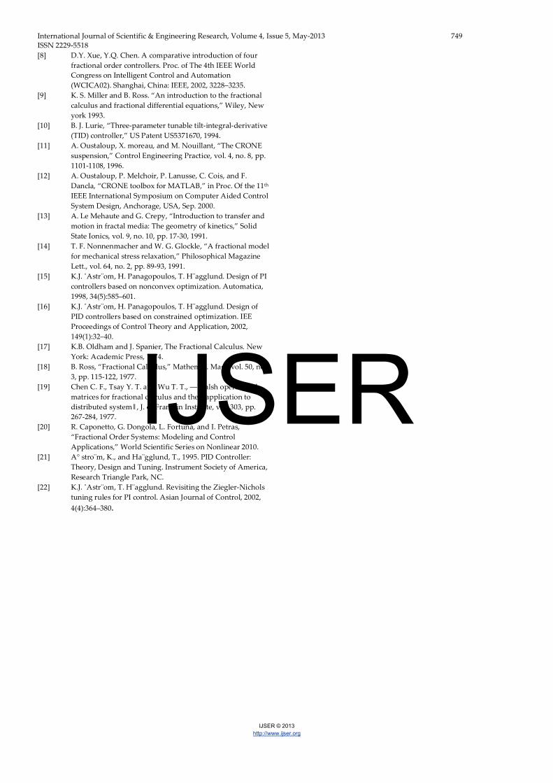
Fig. 5 Lag Dominant system response 𝐺3(𝑠)

Fig. 6 Lag Dominant system response 𝐺4(𝑠)

From figures 3 to 6 it is shown that step response and load disturbance response of F-MIGO and NZ method is given and compared. Both graphs show that fractional order controller is more robust and performance wise better that integer order controller.

Figures 3 and 4 are the delay dominant systems and these responses show that F-MIGO controllers systems have better response in comparison with that of integer order systems.

Figures 5 and 6 are the lag dominant systems in these responses we can see that step response and load disturbance responses are better that integer order controller scheme.

6 CONCLUSION AND FUTURE WORKS: The method proposed in this paper is that the fractional order controllers for integer order systems show that the responses have better closed loop performance than the integer order controllers for integer order systems. Fractional order controllers and systems provide the excellent tool for the description of system’s memory and hereditary properties that’s why fractional order controllers and systems have become hot topic in the dynamical research field since last decade. With the use of fractional order controllers we can get minimum steady state error and good closed loop performance of integer order and fractional order systems. In future work design of fractional order 𝑃𝐼𝛼𝐷𝛽 can be considered for both integer order and fractional order systems as well.

REFERENCES [1] J. G. Zeigler, N. B. Nichols. Optimum settings for automatic

controllers. Transactions of ASME, 1942, 64:759–768. [2] H.N. Koivo, J.N. Tanttu. Tuning of PID controllers: survey

of SISO and MIMO techniques. Proceedings of Intelligent Tuning and Adaptive Control, Singapore, 1991.

[3] S. Yamamoto, I. Hasimoto. Present status and future needs: the view from Japanese industry. In Arkun and Ray ed Proceedings of 4th International Conference on Chemical Process Control, Texas, 1991.

[4] I. Podlubny. Fractional Differential Equations,Mathematics in Science and Engineering, volume 198. San Diego: Academic Press, 1999.

[5] L. Debnath. A brief historical introduction to fractional calculus. Int J Math Educ Sci Technol, 2004, 35(4):487–501.

[6] R.L. Magin. Fractional calculus in bioengineering. Critical ReviewsTM in Biomedical Engineering, 2004, 32(1-4).

[7] B. M. Vinagre, Y. Q. Chen. Lecture Notes on Fractional Calculus Applications in Automatic Control and Robotics. The 41st IEEE CDC2002 Tutorial Workshop # 2. Las Vegas, Nevada,

IJSER



IJSER © 2013


[8] D.Y. Xue, Y.Q. Chen. A comparative introduction of four fractional order controllers. Proc. of The 4th IEEE World Congress on Intelligent Control and Automation (WCICA02). Shanghai, China: IEEE, 2002, 3228–3235.

[9] K. S. Miller and B. Ross. “An introduction to the fractional calculus and fractional differential equations,” Wiley, New york 1993.

[10] B. J. Lurie, “Three-parameter tunable tilt-integral-derivative (TID) controller,” US Patent US5371670, 1994.

[11] A. Oustaloup, X. moreau, and M. Nouillant, “The CRONE suspension,” Control Engineering Practice, vol. 4, no. 8, pp. 1101-1108, 1996.

[12] A. Oustaloup, P. Melchoir, P. Lanusse, C. Cois, and F. Dancla, “CRONE toolbox for MATLAB,” in Proc. Of the 11th IEEE International Symposium on Computer Aided Control System Design, Anchorage, USA, Sep. 2000.

[13] A. Le Mehaute and G. Crepy, “Introduction to transfer and motion in fractal media: The geometry of kinetics,” Solid State Ionics, vol. 9, no. 10, pp. 17-30, 1991.

[14] T. F. Nonnenmacher and W. G. Glockle, “A fractional model for mechanical stress relaxation,” Philosophical Magazine Lett., vol. 64, no. 2, pp. 89-93, 1991.

[15] K.J. ˚Aström, H. Panagopoulos, T. Hägglund. Design of PI controllers based on nonconvex optimization. Automatica, 1998, 34(5):585–601.

[16] K.J. ˚Aström, H. Panagopoulos, T. Hägglund. Design of PID controllers based on constrained optimization. IEE Proceedings of Control Theory and Application, 2002, 149(1):32–40.

[17] K.B. Oldham and J. Spanier, The Fractional Calculus. New York: Academic Press, 1974.

[18] B. Ross, “Fractional Calculus,” Mathemat. Mag., vol. 50, no. 3, pp. 115-122, 1977.

[19] Chen C. F., Tsay Y. T. and Wu T. T., ―Walsh operational matrices for fractional calculus and their application to distributed system‖, J. of Franklin Institute, vol. 303, pp. 267-284, 1977.

[20] R. Caponetto, G. Dongola, L. Fortuna, and I. Petras, “Fractional Order Systems: Modeling and Control Applications,” World Scientific Series on Nonlinear 2010.

[21] A° stro¨m, K., and Ha¨gglund, T., 1995. PID Controller: Theory, Design and Tuning. Instrument Society of America, Research Triangle Park, NC.

[22] K.J. ˚Aström, T. Hägglund. Revisiting the Ziegler-Nichols tuning rules for PI control. Asian Journal of Control, 2002, 4(4):364–380.

IJSER


Documents

Design of Fractional-Order PIa Controller For Integer