- 1 -

Keynote Paper presented at the International Workshop

The Benchmarking of CFD Codes for Application to Nuclear Reactor Safety

Sponsored by the Committee on the Safety of Nuclear Installations

Nuclear Energy Agency Munich, Germany

September 5-7, 2006

Design of and Comparison with Verification and Validation Benchmarks

William L. Oberkampf Validation and Uncertainty Estimation Department

wloberk@sandia.gov

Timothy G. Trucano Optimization and Uncertainty Estimation Department

tgtruca@sandia.gov Sandia National Laboratories

Albuquerque, New Mexico 87185-0828

- 2 -

Abstract

Verification and validation (V&V) are the primary means to assess accuracy and reliability of computational simulations. V&V methods and procedures have fundamentally improved the credibility of simulations in several high-consequence application areas, such as, nuclear reactor safety, underground storage of nuclear waste, and safety of nuclear weapons. Although the terminology is not uniform across engineering disciplines, code verification deals with the assessment of the reliability of the software coding and solution verification deals with the numerical accuracy of the solution to a computational model. Validation addresses the physics modeling accuracy of a computational simulation by comparing with experimental data. Code verification benchmarks and validation benchmarks have been constructed for a number of years in every field of computational simulation. However, no comprehensive guidelines have been proposed for the construction and use of V&V benchmarks. Some fields, such as nuclear reactor safety, place little emphasis on code verification benchmarks and great emphasis on validation benchmarks that are closely related to actual reactors operating near safety-critical conditions. This paper proposes recommendations for the optimum design and use of code verification benchmarks based on classical analytical solutions, manufactured solutions, and highly accurate numerical solutions. It is believed that these benchmarks will prove useful to both in-house developed codes, as well as commercially licensed codes. In addition, this paper proposes recommendations for the design and use of validation benchmarks with emphasis on careful design of building-block experiments, estimation of experiment measurement uncertainty for both inputs and outputs to the code, validation metrics, and the role of model calibration in validation. It is argued that predictive capability of a computational model is built on both the measurement of achievement in V&V, as well as how closely related are the V&V benchmarks to the actual application of interest, e.g., the magnitude of extrapolation beyond a validation benchmark to a complex engineering system of interest.

- 3 -

1. Introduction 1.1 Background

The importance of computer simulations in the design and performance assessment of

engineered systems has increased dramatically during the last three or four decades. The systems of interest include existing or proposed systems that operate, for example, at design conditions, off-design conditions, and failure-mode conditions in accident scenarios. The role of computer simulations is especially critical if we are interested in the reliability, robustness, or safety of high-consequence systems that cannot ever be physically tested in a fully representative environment. Examples are the catastrophic failure of a full-scale containment building for a nuclear power plant, unusual environments or damaged hardware of the US Space Shuttle, long-term underground storage of nuclear waste, and a nuclear weapon involved in a transportation accident. In many situations, it is even difficult to specify what a “representative environment” actually means in complex system. However, computer simulations are beneficial to improved understanding of the response of the system, in the development of public policy, the preparation of safety procedures, and the determination of legal liability. With this increased responsibility, we believe the credibility of the computational results must be raised to a higher level than has been accepted during the early decades of computational simulation. From a historical perspective, we must realize that we are in the early days of changing from an engineering culture of build-test-fix, to a culture based on virtual reality. To have justified confidence in this evolving culture, major improvements must be made in the transparency and visibility of both the maturity of the computer codes used, as well as the uncertainty assessment of the physics models used. Stated more bluntly, we need to move from a culture of glossy marketing and arrogance, to a culture that forthrightly addresses the limitations, weaknesses, and uncertainty of our simulations.

Developers of computational software, computational analysts, and users of the results of simulations face a critical question: How should confidence in computational science and engineering (CS&E) be critically assessed? Verification and validation (V&V) of computational simulations are the primary building blocks for assessing and quantifying this confidence. Briefly, verification is the assessment or estimation of the numerical accuracy of the solution to a given computational model. Validation is the assessment of the accuracy of a computational model through comparison of computational simulations with experimental data. In verification, the association or relationship of the simulation to the real world is not an issue. In validation, the relationship between computation and the real world (experimental data) is the issue.

The nuclear reactor safety community has a long history of contributing to the intellectual foundations of V&V and uncertainty quantification (UQ). The risk assessment community in its dealings with underground storage of nuclear waste has also made significant contributions to the field of UQ. However, contributions from both of these communities to V&V&UQ have concentrated on software quality assurance procedures, as well as statistical procedures for uncertainty estimation. It is fair to say that computationalists (code users and code developers) and experimentalists in the field of fluid dynamics have been pioneers in the development of terminology, methodology and procedures for V&V. The (only) book in the field on V&V provides a good summary of the development of many of the methodologies and procedures in computational fluid dynamics (CFD).[1] Also, Refs. [2-5] provide a comprehensive review of the history and development of V&V from the perspective of the CFD community.

To achieve the next level in credibility of computational simulations will require concerted and determined efforts by individuals, universities, corporations, governmental agencies,

- 4 -

commercial code development companies, engineering societies, and standards-writing organizations throughout the world. The goal of these efforts should be to improve the quality of: the physics models used, the reliability of the computer software, the numerical accuracy estimation, the uncertainty quantification, and the training and expertise of users of the codes. In addition, new methods are critically needed for effectively communicating the maturity and reliability of each of these elements, especially in relationship to decision making on high-consequence systems. This paper will focus on one aspect of needed improvements to code quality and physics model accuracy assessment, specifically, the construction and use of highly demanding V&V benchmarks. The benchmarks of interest here are those relating to accuracy and reliability of codes and physics models. We are not interested here in benchmarks that relate to performance issues, such as, computing speed of codes or performance of codes on different types of computer hardware and operating systems.

Probably the most widely known V&V benchmarks have been developed over the last two decades by the National Agency for Finite Element Methods and Standards (NAFEMS).[6] Roughly 30 verification benchmarks have been constructed by NAFEMS primarily in solid mechanics, but more recently in fluid dynamics. Most NAFEMS verification benchmarks consist of an analytical solution, or an accurate numerical solution, to a simplified physical process described by a partial differential equation. The NAFEMS benchmark set is carefully defined, numerically demanding, and well documented. However, these benchmarks are, at the present time, very restricted in their coverage of various mathematical and/or numerical difficulties, and also their coverage of physical phenomena. In addition, how well a given code performs on the benchmark is left to the interpretation of the user of the code. It would also be expected that the code performance on the benchmark would depend on the experience and skill of the user.

Several large commercial code companies dealing with solid mechanics have developed an extensive set of verification benchmarks that are well documented and can be exercised by licensed users of the code. Such benchmarks are intended to be applied to that specific code, and reflect the dissemination limitations of this information. Documented performance on the benchmarks can be clearly compared with user-independent checks of the same benchmarks. This activity promotes a stronger user understanding of what is minimally expected from performance of these codes. Some examples of these commercial codes are: ANSYS with roughly 250 verification test cases and ABAQUS with roughly 300 test cases. The careful description and extensive documentation of the ANSYS and ABAQUS benchmark set is impressive. However, the primary goal in essentially all of these documented benchmarks is to demonstrate “engineering accuracy” of the codes; not to precisely and carefully quantify the numerical error in the solutions. As stated in one set of documentation: “In some cases, an exact comparison with a finite-element solution would require an infinite number of elements and/or an infinite number of iterations separated by an infinitely small step size. Such a comparison is neither practical nor desirable.” We disagree with this viewpoint on all counts: a) it does not require an infinite number of elements, or iterations, or infinitely small time step, and b) It is practical and desirable to carefully assess the accuracy of a code by comparison with theoretically demanding solutions. We will support our viewpoint in the body of this paper.

Noticeably absent from our list of commercial codes are CFD software packages. A recent paper by Abanto et al[7] tested three unnamed commercial CFD codes on relatively simple verification test problems. The poor results of the codes were shocking to some people, but not to the authors of the paper, nor to us. Although we have not surveyed all of the major commercial CFD codes available, of those examined, we have not found extensive, formally documented, verification or validation benchmark sets for these codes.

- 5 -

A number of efforts have been undertaken in the development of validation databases that could mature into well-founded benchmarks. In the United States the NPARC Alliance has developed a validation database that has roughly twenty different flows.[8] In Europe, starting in the early 1990’s, there has been a much more organized effort in the development of validation databases, primarily focused in aerospace applications. ERCOFTAC (the European Research Community on Flow, Turbulence and Combustion) has collected a number of experimental datasets for validation.[9] QNET-CFD is a Thematic Network on Quality and Trust for the industrial applications of CFD.[10] This network has more than 40 participants from several countries who represent research establishments and many sectors of the industry, including commercial CFD software companies. For a history and review of the various efforts, see Rizzi and Vos[11] and Vos et al.[12]

An observation that the present authors make of this work in validation databases is that many of the database cases are for very complex flows, sometimes referred to as “industrial applications.” Our experience with attempts at validation for complex physical processes, and our observations of many open literature activities, is that the computational results commonly do not compare well with the experimental measurements. Then the activity usually becomes a model calibration activity, or the computational analysts start pointing accusatory fingers at the experimentalists about either what is wrong with their data, or what they should have measured to make the data more effective for validation. A calibration activity can be a useful and pragmatic path forward for use of the calibrated model in future predictions that are very similar to the experimental database. However, calibration does not address the root causes of the weaknesses of the models because there are typically so many modeling approximations, or deficiencies, that could be contributing to the disagreement. We are of the view that calibration should be undertaken from a defined understanding of, or as a response to, V&V assessment; not as a replacement for V&V assessment.[13-15]

As will be discussed in more detail in Section 2.3, Validation Activities, the construction and use of validation benchmarks is much more difficult than verification benchmarks. The primary difficulty in constructing validation benchmarks is that experimental measurements in the past have rarely been designed to provide true validation benchmark data. Refs. [2-4, 16-18] give an in-depth discussion of the characteristics of validation experiments, as well as an example of a wind tunnel experiment that was specifically designed to be a true validation benchmark. The validation benchmarks that have been complied and documented by organized efforts are indeed instructive and useful to users of the codes and to physics model developers. However, we argue in this paper that much more needs to be incorporated into the validation benchmarks, both experimentally and computationally, to achieve the next level of usefulness and impact.

In Ref. [5], the concept of strong-sense V&V benchmarks was introduced. Oberkampf et al argued that strong-sense benchmarks should be of a quality that they be viewed as engineering reference standards. It is these authors’ experience that when there is disagreement with a benchmark, especially a validation benchmark, then the debate shifts to either a) questioning how good the benchmark is, instead of critically examining the simulations that are being compared with the benchmark, or b) how might physical or numerical parameters be adjusted to best match the experimental data. They stated that strong-sense benchmarks are test problems that have the following four characteristics: a) the purpose of the benchmark is clearly understood, b) the definition and description of the benchmark is precisely stated, c) specific requirements are stated for how comparisons are made with the results of the benchmark, and d) acceptance criteria for comparison with the benchmark are defined. In addition, they required

- 6 -

that information on each of these characteristics be “promulgated”, i.e., the information is well documented and publicly available. They asserted that strong-sense benchmarks (SSB) do not presently exist in computational physics or engineering. They suggested that professional societies, academic institutions, governmental organizations, or newly formed, nonprofit, organizations would be the most likely to construct SSBs. This paper builds on these basic ideas and provides detailed recommendations for the characteristics of V&V SSBs, and suggestions how computational simulations could be compared with the SSBs.

1.2 Outline of the Paper

Section 2 begins with a brief review of terminology and how different communities have

varying interpretations of verification and validation. We then discuss how code verification is composed of both numerical algorithm verification activities and software quality assurance practices. It is pointed out that solution verification serves a different goal, that is, estimation of numerical discretization error and iterative solution error. Code verification procedures are discussed with regard to the use of highly accurate analytical solutions, manufactured solutions, and numerical solutions as verification benchmarks for codes. It is pointed out that validation can be viewed as composed of two quite different activities; assessment of computational model accuracy by comparison with experiment, and extrapolation of models to applications of interest along with the determination of their adequacy for the application of interest. The concept of a validation hierarchy is discussed along with its importance in assessing computational model accuracy at many different levels of complexity. The required characteristics of validation experiments are discussed, how they are different from traditional experiments, and how they form the central role in validation benchmarks.

Section 3 discusses our recommendations for the design and construction of verification benchmarks. We discuss details of four elements that should be contained in a verification benchmark: a) purpose and scope of the benchmark, b) mathematical description of the benchmark, c) accuracy assessment of the benchmark, and d) documentation of the benchmark. We discuss how each of the elements applies to the four types of benchmarks: analytical solutions, manufactured solutions, numerical solutions to ordinary differential equations, and numerical solutions to partial differential equations. Although we do not recommend that results of comparisons with benchmarks should be included in the benchmark itself, we discuss how formal comparison results could be used and the types of information that should be included in the comparisons. We point out that making the resulting comparisons of codes with suitable benchmarks is an important component of the published literature in computational science and engineering (CS&E) and is necessary for the progressive improvement of numerical methods.

Section 4 discusses our recommendations for the design and construction of validation benchmarks. We discuss details of four elements that should be contained in the validation benchmark: a) purpose and scope of the benchmark, b) description of the benchmark, experimental techniques, and facility, d) uncertainty quantification of benchmark measurements, and d) documentation of the benchmark. We also discuss how one should compare candidate code results with the benchmark results, paying particular attention to issues of: computation of nondeterministic results to determine the uncertainty of system response quantities due to uncertainties in input quantities, computation of validation metrics to quantitatively measure the difference between experimental and computational results, the minimization of model calibration in comparing with validation benchmarks, and the constructive roll of global sensitivity analyses in validation experiments.

- 7 -

Section 5 discusses a diverse set of issues concerning how a V&V benchmark database might be initiated, implemented, and contribute to CS&E. Examples of some of these issues are: primary and secondary goals of the database; initial construction of an internet-based system; software construction of the database; review and approval procedures for entries into the database; open versus restricted use of the database; organizational control of the database; and, possible initial and long term funding of the database.

Closing remarks and possible future steps toward construction of a V&V benchmark database are given in Section 6.

2. Review of Verification and Validation Processes

There are a wide variety of different meanings used for V&V in the various technical

disciplines. The Institute of Electrical and Electronics Engineers (IEEE) was the first major engineering society to develop formal definitions for V&V.[19] These definitions, initially published in 1984, were adopted and associated procedures were developed by the software quality assurance community, the International Organization for Standardization (ISO), and the nuclear reactor safety community.[20, 21] After a number of years of discussion and intense debate in the US defense and CFD communities, these definitions were found to be of limited value. In particular, these definitions did not speak directly to certain issues that are of particular importance in CS&E, such as the dominance of algorithmic issues in the numerical solution of partial differential equations, and the importance of comparisons of computational results with the “real world”. As a result, the US Department of Defense, developed an alternate set of definitions.[22, 23] Following with more precisely targeted definitions, the American Institute of Aeronautics and Astronautics (AIAA) and the American Society of Mechanical Engineers (ASME) adopted the following definitions:[13, 14]

Verification: The process of determining that a model implementation accurately represents

the developer’s conceptual description of the model and the solution to the model. Validation: The process of determining the degree to which a model is an accurate

representation of the real world from the perspective of the intended uses of the model. These definitions have also been recently adopted by the United States Department of Energy National Nuclear Security Administration’s (NNSA) Advanced Simulation and Computing program (ASC).[24] For a detailed discussion of the history of the development of the terminology from the perspective of the CS&E communities, see Refs. [4, 5, 25, 26].

Verification provides evidence, or substantiation, that the conceptual model is solved correctly by the computer code in question. In CS&E the conceptual model, sometimes called the mathematical model, is typically defined by a set of partial differential or integro-differential equations, along with the required initial and boundary conditions. The computer code solves the computational model, i.e., the discrete-mathematics version, or mapping, of the conceptual model. The fundamental strategy in verification is to identify, quantify, and reduce errors caused by the mapping of the conceptual model to a computer code. Verification does not address the issue of whether the conceptual model has any relationship to the real world, e.g., physics.

Validation, on the other hand, provides evidence, or substantiation, for how accurately the computational model simulates the real world for system responses of interest. The US Department of Defense, and many other organizations, must deal with complex systems

- 8 -

composed of physical processes, computer controlled subsystems, and strong human interaction. From their perspective, assessment of accuracy compared to the real world would include expert opinion and well-founded knowledge of experienced professionals. From the perspective of CS&E community, the real world is traditionally viewed to only mean experimentally measured quantities in a physical experiment.[13, 14] Validation activities presume that the discrete-mathematics version of the model, which is solved by the computer code, is an accurate solution of the conceptual model. However, programming errors in the computer code, numerical algorithm deficiencies, or inaccuracies in the numerical solution, for example, may cancel one another in specific validation calculations and give the illusion of an accurate solution. Verification, thus, should be accomplished before the validation process begins so that one’s assessment of mathematical accuracy is not influenced by whether the agreement of the computational results with experimental data is “good” or “bad.” While verification is not simple, it is conceptually less complex than validation because it deals with mathematics and computer science issues. Validation, on the other hand, must address a much broader range of issues: assessment of the fidelity of the mathematical modeling of physical processes, assessment of consistency, or relevancy, of the mathematical model to the physical experiment being conducted, the influence of experimental diagnostic techniques on the measurements themselves, and estimation of experimental measurement uncertainty. Validation rests on evidence that the correct experiments were executed correctly, as well as evidence of mathematical accuracy of the computed solution, These problems are practically coupled in non-trivial ways in complex validation problems although they are logically distinct. As Roache[1] succinctly states, “Verification deals with mathematics; validation deals with physics.”

2.1 Verification Activities

2.1.1 Fundamentals of Verification

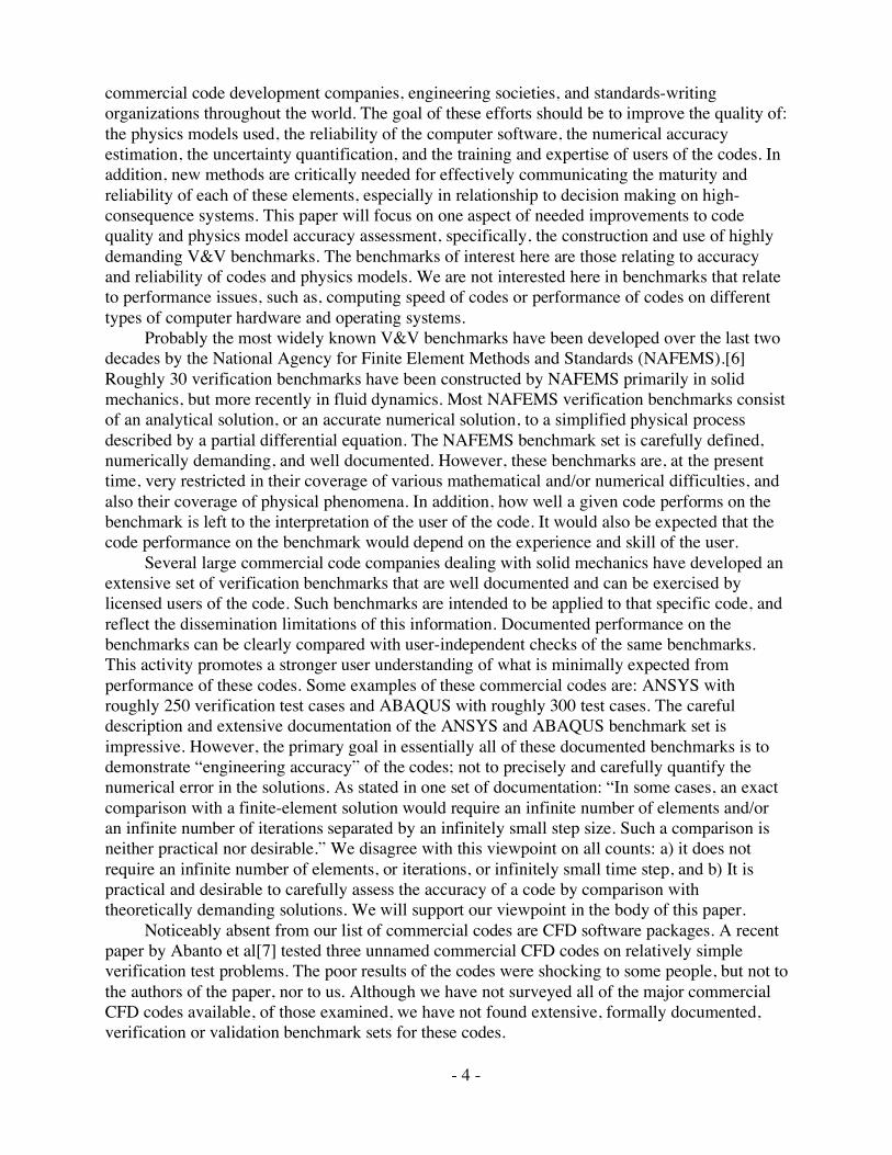
Two types of verification are generally recognized and defined in computational simulation: code verification and solution verification.[1, 27] Recent work by Ref. [4] argues that code verification should be further segregated into two parts: numerical algorithm verification and software quality assurance (SQA). See Fig. 1. Numerical algorithm verification addresses the software reliability of the implementation of all of the numerical algorithms that affect the numerical accuracy and efficiency of the code. The major goal of numerical algorithm verification is to accumulate sufficient evidence to demonstrate that the numerical algorithms in the code are implemented correctly and functioning as intended. SQA emphasizes determining whether or not the code, as a part of a software system, is reliable (implemented correctly) and produces repeatable results on specified computer hardware and a specified software environment, including compilers, libraries, etc. SQA procedures are primarily needed during software development, testing, and modification, and secondarily during production-computing operations.

- 9 -

Figure 1 Integrated View of Code Verification in Computational simulation

[5]

Unfortunately, as discussed in Ref. [28], when solving complex partial differential equations the distinct problems of mathematical correctness, algorithm correctness, and software implementation correctness are virtually impossible to decouple. For example, algorithms often represent non-rigorous mappings of mathematical approximations to the underlying discrete equations. Two examples are approximate factorization of difference operators and algorithms that are derived assuming high levels of continuity, when in reality they are applied to problems with little or no continuity of derivatives. Whether these algorithms are “correct” cannot be assessed in isolation from code executions, which are in turn coupled to software implementation. One consequence is that an “obvious” numerical inaccuracy may not be easily associated with one of mathematics, algorithms, or software. This suggests a greater overlap between SQA and the “science” of numerical computation than some practitioners feel comfortable with.

Numerical algorithm verification, SQA, and solution verification are fundamentally empirical. Specifically, these issues are based on observations, comparisons, and analyses of the code results for specific input options chosen. Numerical algorithm verification centers on careful investigations of topics such as spatial and temporal convergence rates, iterative convergence, independence of solutions to coordinate transformations, and symmetry tests related to various types of boundary conditions. Analytical or formal error analysis is inadequate in numerical algorithm verification because the code must demonstrate the analytical and formal results of the numerical analysis. Numerical algorithm verification is conducted by comparing computational solutions with highly accurate solutions. We believe Roache’s description of this as “error evaluation” clearly distinguishes it from numerical error estimation.[29] Solution verification centers on estimating the numerical error for particular applications, e.g., different mesh resolutions, when the correct solution is not known.

SQA procedures are very well developed, as they have been in existence for at least three

- 10 -

decades. They are a combination of software management, inspection, and testing procedures. However, there is ongoing debate about the precise role of SQA in CS&E, as well as on the efficacy of particular SQA strategies and methods.[28, 30, 31] Trucano et al.[28] emphasize three areas that are ripe for developing precise overlap between SQE and CS&E V&V: (1) testing; (2) software lifecycle definition; and (3) code accreditation. The latter issue is firmly in the orbit of the current paper, although we do not explicitly discuss it.

Fig. 1 depicts a top-down process with two main branches of code verification: numerical algorithm verification and SQA practices.[5] Numerical algorithm verification, discussed in Section 2.1.2, focuses on the accumulation of evidence to demonstrate that the numerical algorithms in the code are implemented correctly and functioning properly. The main technique used in numerical algorithm verification is testing, which is alternately referred to in this paper as numerical algorithm testing or algorithm testing. SQA activities include practices, procedures and processes primarily developed by researchers and practitioners in the computer science and IEEE communities. Conventional SQA emphasizes processes (management, planning, acquisition, supply, development, operation, and maintenance), as well as reporting, administrative, and documentation requirements. One of the key elements of SQA is configuration management of the software: configuration identification, configuration and change control, and configuration status accounting. These activities are primarily directed toward programming correctness in the source program, system software, and compiler software. As shown in Fig. 1, software quality analysis and testing can be divided into static analysis, dynamic testing, and formal analysis. Dynamic testing further divides into such elements of common practice as regression testing, black-box testing, and glass-box testing. From a SQA perspective, one could reorganize Fig. 1 such that all of the activities listed on the left, under Numerical Algorithm Verification, could be moved under dynamic testing. However, the computer science and IEEE communities have shown no formal interest in the development of these activities. These activities, on the other hand, dominate code development practice in the traditional CS&E communities.

A recent comprehensive analysis of the quality of scientific software by Hatton[32] documented, to the disbelief of many, a dismal picture of code verification. Hatton studied more than 100 scientific codes over a period of seven years using both static analysis and dynamic testing. The codes were submitted primarily by companies, but also by government agencies and universities from around the world. These codes covered 40 application areas, including graphics, nuclear engineering, mechanical engineering, chemical engineering, civil engineering, communications, databases, medical systems, and aerospace. Both safety-critical and non-safety-critical codes were comprehensively represented. All codes were “mature” in the sense that the codes were regularly used by their intended users, i.e., the codes had been approved for production use. The total number of lines of code analyzed in Fortran 66 and 77 was 1.7 million and the total number of lines analyzed in C was 1.4 million. As the major conclusion in his study, Hatton stated, “The T experiments suggest that the results of scientific calculations carried out by many software packages should be treated with the same measure of disbelief researchers have traditionally attached to the results of unconfirmed physical experiments.” Hatton’s conclusion is disappointing, but not at all surprising in our view.

Solution verification centers on the quantitative estimation of the numerical accuracy of a given solution to the PDEs. Because, in our opinion, the primary emphasis in solution verification is significantly different from that in numerical algorithm verification and SQA, we believe solution verification should be referred to as numerical error estimation. That is, the primary goal is attempting to estimate the numerical accuracy of a given solution, typically for a

- 11 -

nonlinear PDE with singularities and discontinuities. Assessment of numerical accuracy is the key issue in computations used for validation activities, as well as in use of the code for the intended application. Numerical error estimation is strongly dependent on the quality and completeness of code verification.

The two basic approaches for estimating the error in a numerical solution to a PDE are a priori and a posteriori error estimation techniques. An a priori approach uses only information about the numerical algorithm that approximates the partial differential operators and the given initial and boundary conditions. A priori error estimation is a significant element of classical numerical analysis for PDEs, especially those underlying the finite element and finite volume methods.[1, 33-38] An a posteriori approach uses all of the a priori information, plus computational results from previous numerical solutions, e.g., solutions using different mesh resolutions or solutions using different order of accuracy methods. We believe the only quantitative assessment of numerical error that can be achieved in practical cases of nonlinear, complex, PDEs is through a posteriori error estimates.

A posteriori error estimation has primarily been approached through the use of either Richardson extrapolation[1] or estimation techniques based on finite element approximations.[39, 40] Richardson extrapolation uses solutions on multiply refined meshes to estimate the spatial discretization error. It can also be used on multiply refined time-step solutions to estimate temporal discretization error. Richardson’s method can be applied to any discretization procedure for differential or integral equations, e.g., finite difference methods, finite element methods, finite volume methods, spectral methods, and boundary element methods. As pointed out by Roache,[1] Richardson’s method produces different estimates of error and uses different norms than the traditional a posteriori error methods used in finite elements.[35, 41] A Grid Convergence Index (GCI), based on Richardson’s extrapolation, has been developed by Roache to assist in the estimation of grid convergence error.[1, 42, 43]

Although SQA and solution verification are quite important, a detailed discussion of these topics is beyond the scope of this paper. For further discussion of SQA issues, see, for example, Refs. [5, 44-46]. For further discussions of numerical error estimation, see, for example, Refs. [1, 33-38, 47-50].

2.1.2 Code Verification Procedures

From the perspective of the numerical solution of PDEs, the major components of code verification include the definition of appropriate benchmarks for evaluating solution accuracy and the determination of satisfactory performance of the algorithms on the benchmarks. Code verification rests upon comparing computational solutions to the “correct answer,” which is provided by highly accurate solutions for a set of well-chosen benchmarks. The correct answer can only be known in a relatively small number of isolated cases. These cases therefore assume a very important role in verification and should be carefully formalized in test plans for verification assessment of the code.

Figure 2 depicts a method for detecting numerical algorithm deficiencies and programming errors by using verification benchmarks. The conceptual model, or mathematical model, is derived from the physics of interest and the mathematical assumptions made in constructing the model. Since we are interested in benchmark solutions, the conceptual model is chosen by what exact or highly accurate solutions are known, or new ones that can be generated. The conceptual model is typically given by a set of PDEs and all of the associated input data, e.g., initial conditions, boundary conditions, material properties, nuclear cross-sections, etc. These equations are discretized, i.e., mapped from derivatives and integrals to algebraic equations, using the

- 12 -

numerical algorithms chosen. The discretized equations are programmed in the computer code. When the code is exercised by solving the benchmark problem, then the code produces computational results of interest. The results from the code are then compared with the benchmark solution results to evaluate the differences that occur. The comparisons are usually examined along boundaries of interest or error norms computed over the entire solution domain. The accuracy of each of the dependent variables or functionals of interest can be determined as part of the comparisons.

Figure 2 Method to Detect Sources of Errors in Code Verification

Probably the most important issue in the design and computation of verification

benchmarks is the mathematical accuracy of the benchmark solution. The AIAA Guide,[13] suggests the following hierarchical organization of confidence or accuracy of benchmarks (from highest to lowest): (1) analytical solutions, (2) highly accurate ordinary differential equation numerical solutions, and (3) highly accurate numerical solutions to PDEs. Analytical solutions are closed-form solutions to special cases of the PDEs that define the conceptual model. These closed-form solutions are commonly represented by infinite series, complex integrals, and asymptotic expansions. Relatively simple numerical methods are usually used to compute the infinite series, complex integrals, and asymptotic expansions in order to obtain the solutions of interest. The accuracy of these solutions, particularly if they are infinite series or asymptotic expansions, must be carefully quantified, which can be very challenging. The most significant practical shortcoming of classical analytical solutions is that they exist only for very simplified physics, material properties, and geometries.

The second type of highly accurate solution is the numerical solution to special cases of the general PDEs that can be mathematically simplified to ordinary differential equations (ODE). The ODEs can be either initial value problems or boundary value problems. These solutions

- 13 -

commonly result from simplifying assumptions, such as simple geometries that allow formation of similarity variables. Once an ODE is obtained, then a highly accurate ODE solver can compute the numerical solution. Highly accurate ODE solvers typically employ both variable integration-step and variable order of accuracy numerical methods. In fluid dynamics, some well known ODE benchmarks are stagnation point flow, laminar flow in two and three dimensions, Taylor-Maccoll solution for inviscid flow over a sharp cone, and Blasius solution for laminar flow over a flat plate. Note that the Blasius solution would be a useful benchmark for assessing the accuracy of CFD code that solves the boundary layer equations. However, it would not be a good benchmark for testing a Navier-Stokes code because the Blasius solution also relies on the approximations assumed in the boundary layer theory. As would be expected, there would be a difference between a highly accurate Blasius solution and a highly accurate Navier-Stokes solution because of the different modeling assumptions involved in each. The modeling assumptions must be the same between the benchmark solution and the code being tested. The only question that should be answered in Fig. 2 is related to numerical accuracy and correctness of the code being tested.

The third type of highly accurate solution is numerical solution to more complex PDEs, i.e., more complex than those obtained from analytical solutions or ODE numerical solutions. The accuracy of these type benchmark solutions clearly becomes a more questionable issue compared to analytical solutions or ODE solutions. In the literature, for example, one can find descriptions of computational simulations that are considered to be “benchmark solutions” by the author, but are later found to be lacking. Although it is common practice to conduct code-to-code comparisons, we argue that these types of comparisons are of very limited value unless highly demanding requirements are imposed on the numerical solution that is considered as the “benchmark.”[51] These requirements will be discussed in detail in section 3.1

During the last decade a technique has been developed for constructing a special type of analytical solution that is specifically used for testing numerical algorithms and computer codes; it is referred to as the “Method of Manufactured Solutions” (MMS).[1, 52] The MMS is a method of custom-designing verification benchmarks of wide applicability, where a specific form of the solution function is assumed to satisfy the PDE of interest, rather than a major simplification of the PDE of interest. This function is inserted into the PDE, and all the derivatives are analytically derived. Typically these derivatives are derived by using symbolic manipulation software such as MATLAB® or Mathematica®. The equation is rearranged such that all remaining terms in excess of the terms in the original PDE are grouped into a forcing-function or source term. This source term is then added to the original PDE so that the assumed solution function satisfies the new PDE exactly. When this source term is added to the original PDE, one recognizes that we are no longer dealing with physically meaningful phenomena, although we remain in the domain of mathematical interest. This realization can cause some researchers or analysts to claim that the solution is no longer relevant to computational simulation. The fallacy of this argument is emphasized by noting that in verification we are only dealing with testing of the numerical algorithms and coding: not the relationship of the code results to physical responses of the system. Since the solution to the modified PDE was “manufactured”, the boundary conditions for the new PDE are analytically derived from the solution chosen. For the three types of common boundary conditions, one can use the chosen solution function to: a) simply evaluate solution on any boundary of interest, i.e., a Dirichlet condition, b) analytically derive a Neumann type boundary condition and apply it on any boundary, and c) analytically derive a boundary condition of the third kind and apply it on any boundary. MMS could be described as finding the problem, i.e., the PDE, for which we have

- 14 -

assumed a solution. Using MMS in code verification requires the ability to insert the analytically derived source

term and boundary conditions into the code being tested, and that this insertion be verified in the sense of code verification. This technique verifies a large number of numerical aspects in the code, such as, the numerical method, differencing or finite element technique, spatial-transformation technique for grid generation, grid-spacing technique, and correctness of algorithm coding. Although the MMS has been used in various forms for checking computer codes for a number of years, recent extensions and generalizations of the method have proven very effective. As pointed out by a number of researchers in this topic, solutions in MMS must be carefully chosen to achieve the desired test results. For example, solutions should be chosen so that as many terms as possible in the original PDE are brought into play. This includes any submodels affecting terms in the original PDE, as well as any mathematical transformations of physical space to computational space. MMS has proven to be so effective that we will specifically add it to the list of three types of highly accurate solutions described earlier in this section.

In code verification the key feature to determine is the observed, or demonstrated, order of accuracy from multiple numerical solutions. As discussed in a number of references,[1, 52] Richardson extrapolation is used in combination with the known exact solution and results from two different mesh resolutions to determine the observed order of accuracy from a code. A typical plot of observed order of accuracy versus mesh resolution is shown in Fig. 3. When the mesh is sufficiently resolved, the numerical solution enters the asymptotic convergence region with regard to spatial resolution. In this region the observed order of accuracy becomes a constant. By computing the observed order of accuracy in testing a code one can make two strong statements concerning accuracy. First, if the observed order is greater than zero, then the code converges to the correct solution as the mesh is refined. If the observed order of accuracy is zero, then the code will converge to an incorrect answer. Second, if the observed order of accuracy matches (or nearly matches) the formal order of accuracy, then the code demonstrates that it can reproduce the theoretical order of accuracy of the numerical method. This statement belies the fact that in many practical cases, the theoretical order of accuracy of a complex code is actually not known rigorously, or it is a mixed order scheme. When an empirical convergence study is in disagreement with a claimed formal order of accuracy, it may be the case that both sides of this comparison must be subject to close analysis.

- 15 -

Figure 3

Observed order of accuracy as a function of mesh resolution for two Navier-Stokes codes[53]

Researchers have found a number of reasons why the observed order of accuracy can be

less than the formal accuracy when the latter is rigorously known. Some of the reasons are: (1) a programming error exists in the computer code, (2) the numerical algorithm is deficient is some way, (3) insufficient grid resolution so that the grid is not in the asymptotic convergence region of the power series expansion for the particular system response quantity (SRQ) of interest, (4) the formal accuracy for interior grid points is different than the formal accuracy for boundary conditions with derivatives resulting in a mixed order of accuracy, (5) singularities, discontinuities, and contact surfaces interior to the domain of the PDE, (6) singularities and discontinuities in the boundary conditions, (7) highly stretched meshes, (8) inadequate convergence of an iterative procedure in the numerical algorithm, and (9) over-specified boundary conditions. It is beyond the scope of this paper to discuss these in detail, however some of the representative references in these topics are [1, 33, 52, 54-63]. For the types of benchmarks we will concentrate on in this paper, we will focus on testing candidate codes for reasons (1) – (4).

2.2 Validation Activities

2.2.1 Fundamentals of Validation

Various researchers and engineering standards documents[4, 5, 13-15, 64] have pointed out that there are two key, and distinct, issues in validation: a) quantification of the accuracy of the conceptual model by comparisons with experimental data, and b) estimation of the accuracy of the conceptual model for its intended use. The definition of validation, given at the beginning of Section 2, is not particularly clear on the issue and, as a result, the definition has been interpreted to include both issues, and also been interpreted to only include the first issue. The first issue is typically referred to as model fidelity assessment, or assessment of validation metrics, and the second issue is usually referred to as adequacy assessment of the model for applications of

- 16 -

interest, or predictive capability estimation. Figure 4 depicts these two issues, as well as the input information these two issues require.

Figure 4 Two Aspects of Model Validation

It is clear from Fig. 4 that model fidelity assessment by comparison of model results to

experimental results is distinctively different from adequacy assessment of the model relative to accuracy requirements for applications that may, or may not, be very well defined. The most recent engineering standards document dealing with V&V, referred to as the ASME Guide[14] takes the view that both aspects of validation are fundamentally combined in the term “validation.” The AIAA Guide,[13] however, takes the view that “validation” only deals with the first aspect; assessment of model accuracy, with no implication that model accuracy is “good” or “bad”. Uncertainty is involved in the assessment, both in terms of experimental measurement uncertainty and in terms of the computational simulation, primarily because input quantities needed from the experiment are not available. The second aspect is regarded as a separate activity related to predictive capability. Stated differently, the AIAA Guide takes the perspective that predictive capability uses assessed model accuracy as input, but predictive capability also incorporates: a) additional uncertainty estimation resulting from extrapolation of the model beyond the existing experimental database to future applications of interest, and b) comparison of the accuracy requirements needed by a particular application relative to the estimated accuracy of the model for that specific applications of interest. Both perspectives are useful and workable, but the terminology clearly means different things and, as a result, one must be careful in discussions and writing on the subject.

Work by the ecological community[65, 66] and recent work by the hydrology community[67] in Europe have independently developed very similar ideas to those being developed in the US with regard to V&V. Rykiel[65] makes a important practical point, especially to analysts and decision makers, concerning the difference between the philosophy of science viewpoint and the practitioner’s view of validation: “Validation is not a procedure for

- 17 -

testing scientific theory or for certifying the ‘truth’ of current scientific understanding … Validation means that a model is acceptable for its intended use because it meets specified performance requirements.” Refsgaard and Henriksen[67] have recommended terminology and fundamental procedures for V&V that are applicable to a much wider range of simulations than just hydrological modeling. Their definition of validation makes the two aspects of validation in Fig. 4 quite clear: “Model Validation: Substantiation that a model within its domain of applicability possesses a satisfactory range of accuracy consistent with the intended application of the model.” An additional crucial issue stressed by Refsgaard and Henriksen, and corroborated by both the AIAA and ASME Guides, is: “Validation tests against independent data that have not also been used for calibration are necessary in order to be able to document the predictive capability of a model.” Stated differently, the key issue in validation is assessment of the model in a “blind” test with experimental data, whereas the key issue in calibration is adjustment of physical modeling parameters to improve agreement with experimental data. It is difficult, and sometimes impossible, to make blind comparisons, e.g., when well-known benchmark validation data is available for comparison. However, we must be extremely cautious in making conclusions of predictive accuracy of models when the analyst has seen the data. Knowing the “correct answer” before hand is extremely seductive, even to a saint.

An additional fundamental, as well as practical, aspect of validation in a real engineering environment has been the introduction of the concept of a validation hierarchy.[13, 14] Because of the infeasibility and impracticality of conducting true validation experiments on most complex or large scale systems, the recommended method (and we would agree that it is logically necessary) is to use a building-block approach. This approach divides the complex engineering system of interest into three or more progressively simpler tiers: subsystem cases, benchmark cases, and unit problems. In the reactor safety field a very similar concept has been used for some time and it is usually referred to as separate effects testing. The strategy in the tiered approach is to assess how accurately the computational results compare with the experimental data at multiple degrees of physics coupling and geometric complexity. The approach is extremely useful in that: (1) it recognizes that there is a hierarchy of complexity in systems, physics and geometry, (2) the hierarchy requires a very wide range of experienced individuals to construct it; often discovering subsystem or component interactions that had not been recognized before, (3) models, or submodels, can be tested at any of the tiers of complexity, and (4) it recognizes that the quantity, accuracy and cost of information that is obtained from experiments varies radically over the range of tiers. Each comparison of computational results with experimental data allows an inference of model accuracy concerning tiers both above and below the tier where the comparison is made. The construction and use of the validation hierarchy is particularly important in situations were the complete system of interest cannot be tested. For example, in the nuclear power industry very similar ideas to the validation hierarchy have been used in safety studies and probabilistic risk assessment for abnormal environment scenarios.

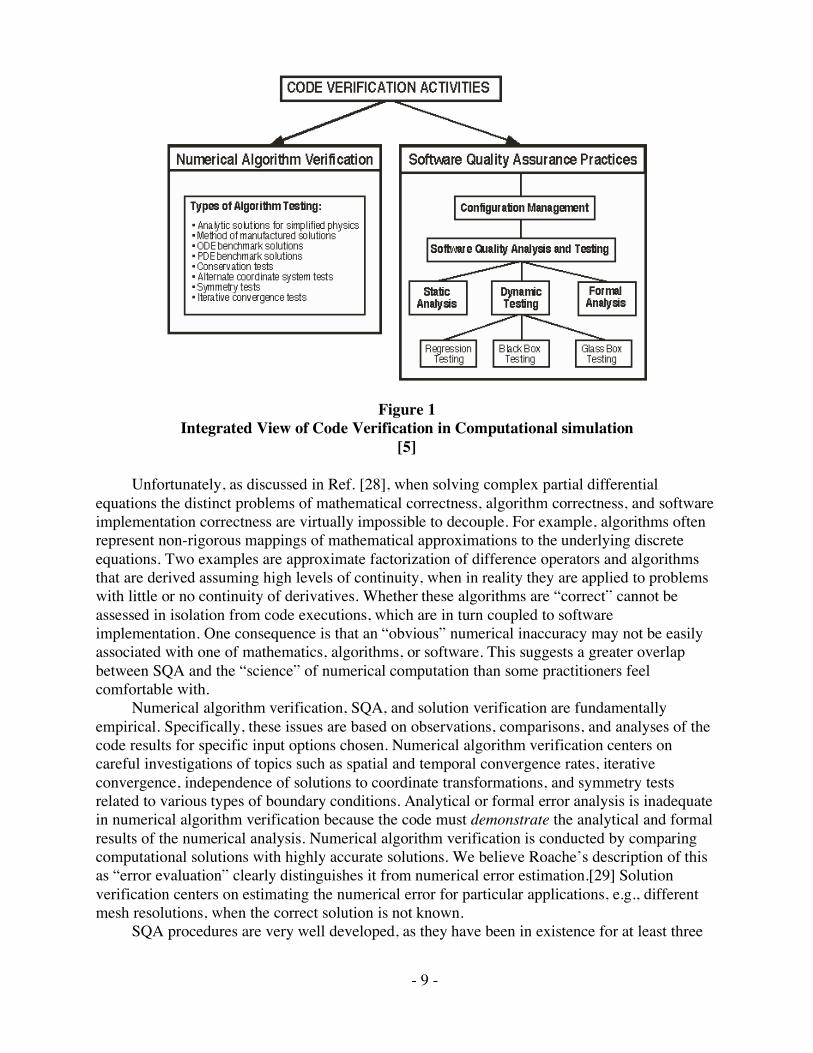
An example of a hierarchical structure for a complex, multidisciplinary system was presented in Ref. [68]. The example features an air-breathing, hypersonic cruise missile. The missile is assumed to have an autonomous guidance, navigation, and control (GNC) system, an on-board optical target seeker, and a warhead. Figure 5 shows the system-level hierarchical validation structure for the hypersonic cruise missile. The missile is referred to as the complete system, and the following are referred to as systems: propulsion, airframe, GNC, and warhead. The hierarchy shown is not unique, nor is it necessarily optimum for every computational-simulation perspective of the missile system. In addition, the structure shown in Fig. 5 focuses on the airframe system and the aero/thermal protection subsystem for the purpose of analyzing the

- 18 -

aero/thermal performance of the missile.

Figure 5

Validation Hierarchy for a Hypersonic Cruise Missile[68]

2.2.2 Characteristics of Validation Experiments With the critical role that validation experiments play in assessment of model accuracy and

predictive capability, it is fair to ask: Exactly what is a validation experiment? Or, How is a validation experiment different from other experiments? In an attempt to answer these questions, we first suggest that traditional experiments could generally be grouped into three categories. The first category comprises experiments that are conducted primarily to improve the fundamental understanding of some physical process. Sometimes these are referred to as physical-discovery experiments. The second category of traditional experiments consists of those conducted primarily for constructing or improving mathematical models of fairly well understood physical processes. Sometimes these are referred to as model calibration experiments. The third category of traditional experiments includes those that determine or improve the reliability, performance, or safety of components, subsystems, or complete systems. These experiments are sometimes called “proof tests” or “system performance tests.”

The present authors and colleagues[2, 3, 16, 69-73] have argued that validation experiments constitute a new type of experiment. A validation experiment is conducted for the primary purpose of determining the predictive accuracy of a computational model, or group of models. In other words, a validation experiment is designed, executed, and analyzed for the

- 19 -

purpose of quantitatively determining the ability of a mathematical model and its embodiment in a computer code to simulate a well-characterized physical process. Thus, in a validation experiment “the code is the customer” or, if you like, “the computational analyst is the customer.” Only during the last 10 to 20 years has computational simulation matured to the point where it could even be considered as a customer in this sense. As modern technology increasingly moves toward engineering systems that are designed, and possibly even fielded, based predominately on CS&E, then CS&E itself will increasingly become the customer of experiments.

We argue that there are three aspects that should be used to optimize the effectiveness and value of validation experiments: (1) early in the planning process, define the goals and the expected results of the validation activity, (2) design the validation experiment by using the code in a predictive sense and also account for the capability limitations of the experimental facility, and (3) develop a well-thought-out plan for analyzing and quantitatively comparing the computational and experimental results.[73] The first aspect, defining the goals and expected results, deals with issues, such as: clear determination how the validation activity relates to the application of interest (typically through the validation hierarchy); identification of what physics modeling issues are being tested; deciding if the validation activity intended to severely test the model or make the model look good; specification of what is required from both the computational and experimental aspects of the validation activity to conclude that each aspect was deemed a “success;” and laying out the steps that would be taken if the model (or the experimental results) looks surprisingly good or surprisingly bad.

In the second aspect above, “design” means using the code to directly guide design features of the experiment, such as: geometry, initial and boundary conditions, material properties, sensor locations, and diagnostic techniques, e.g. strain gauges, thermocouples, optical techniques, and radiation detectors. Even if the accuracy of the code predictions is not expected to be high, the code can frequently guide much of the design of the experiment. Using the code, and the goals of the validation activity, one can also guide the required accuracy needed of the experimental measurements, or the number of experimental realizations needed to obtain a specific statistical result. Suppose, through a series of exploratory calculations for a particular application of the code, an unexpectedly high sensitivity to certain physical parameters is found. If this unexpected sensitivity has an important impact on the application of interest, a change in the design of the validation experiment may be needed, or indeed, a completely separate validation experiment may be called for. Also, the limitation of the experimental facility should be directly factored into the design of the experiment. Examples of facility or diagnostic limitations are: inability to obtain the range of parameters, e.g., load, temperature, velocity, time, radiation flux, needed to meet the goals of testing the model, inability to obtain the needed accuracy of measurements (both system response quantities and model input quantities), and inability to measure all of the needed input quantaties, e.g., initial conditions, boundary conditions, material properties, needed for the code simulation.

The third aspect above refers to the importance of rigorously analyzing and quantitatively comparing the computational and experimental results. As shown in top portion of Fig. 4, this type of quantitative comparison is now called a validation metric and is an active topic of research.[4, 74-79] Validation metrics use statistical procedures to compare the results of code calculations with the measurements of validation experiments. Because we emphasize that the overarching goal of validation experiments is to develop quantitative confidence so that the code can be used for its intended application, we have argued the central role of validation metrics. Stated differently, we believe predictive capability should be built directly on quantitative

- 20 -

measures of agreement that have been demonstrated in previous assessments of the model using experimental data, as opposed to obscure or vague declarations that the model is “valid,” and then making predictions. In the statistical inference literature, there has been a long history of the development of statistical procedures for closely related inference tasks. However, most of these procedures yield either probabilistic measures of agreement, such as hypothesis testing, or they are directed at calibration of models, such as Bayesian updating.

As proposed in Refs. [78, 79], we currently believe that useful validation metrics should include several characteristics. Some of the recommended characteristics concerning a metric are: (1) explicitly include an estimate of the numerical error in the computed system response quantity (SRQ), or exclude the numerical error because it has been demonstrated to be small relative to the measurement uncertainty, (2) include in some explicit way an estimate of the measurement uncertainty in the experimental data for the system response quantities of interest, (3) depend on the number of experimental measurements that have been made of the SRQ, e.g., multiple replications of the measurements of the SRQ, and multiple measurements of a SRQ over a range of input quantities, and (4) exclude any indications, either explicit or implicit, of the level of adequacy of agreement between computational and experimental results. This last recommendation refers to the common practice of declaring the computational results “valid” if the results pass through the uncertainty bands of the experimental measurements.

During the past several years, a group of researchers at Sandia National Laboratories has been developing methodological guidelines and procedures for designing and conducting a validation experiment.[2-4, 16, 69-73] These guidelines and procedures have emerged as part of a concerted effort in the NNSA ASC program to provide a rigorous foundation for V&V for computer codes that are important elements of the U.S. nuclear weapons program.[80] Historically, they were first developed in their current form in a joint computational and experimental program conducted in a wind tunnel, however, they apply over a wide range of CS&E.

Guideline 1: A validation experiment should be jointly designed by experimentalists, model

developers, code developers, and code users working closely together throughout the program, from inception to documentation, with complete candor about the strengths and weaknesses of each approach.

Guideline 2: A validation experiment should be designed to capture the essential physics of interest, including all relevant physical modeling data and initial and boundary conditions required by the code.

Guideline 3: A validation experiment should strive to emphasize the inherent synergism between computational and experimental approaches.

Guideline 4: Although the experimental design should be developed cooperatively, independence must be maintained in obtaining both the computational and experimental results.

Guideline 5: A hierarchy of experimental measurements of increasing computational difficulty and specificity should be made, for example, from globally integrated quantities to local measurements.

Guideline 6: The experimental design should be constructed to analyze and estimate the components of random (precision) and bias (systematic) experimental errors.

These guidelines are applicable to any tier in the validation hierarchy discussed with regard to Fig. 5. A detailed discussion of each of these six guidelines is beyond the scope of the present

- 21 -

work. The reader is referred to the given references for an in-depth discussion of what these guidelines mean, how they can be implemented, and the difficulties that can be encountered. Some of these guidelines will be incorporated into the recommendations for the construction of validation benchmarks, Section 4.1.

3. Recommendations for Verification Benchmarks The discussion of SSBs in verification, as well as in validation, is divided into the

recommended features of the benchmark itself and how one should compare a code being tested (referred to as the candidate code) to the benchmark results. The characteristics we recommend here for SSBs are not discipline specific, but can be applied to many fields of physics and engineering.

3.1 Construction of Verification Benchmarks

As discussed in Section 1.1, Introduction, Ref. [5] suggested three characteristics for the construction of a SSB: a) the purpose of the benchmark should be clearly stated, b) the definition and description of the benchmark should be precisely stated, and c) the benchmark should be well documented. We agree with these characteristics and we add an additional characteristic that should be incorporated in their construction: d) the accuracy of the benchmark should be carefully assessed and the pedigree of the evidence should be explained in detail.

3.1.1 Purpose and Scope of the Benchmark

The description given in the purpose and scope of the benchmark should be a textual description: no equations or symbols. The reason for this is that we believe that an electronic database of verification benchmarks should be constructed in the future, similar to the ideas expressed by Rizzi and Vos discuss.[11] With an electronic database, one could search the database for key words that would assist in finding those benchmarks that could be applicable to particular problems of interest. In addition, the purpose and scope of the benchmark should be described from various perspectives.

The first perspective of the information given in the description is the general class of physical process being modeling in the benchmark. For example, in fluid dynamics the description should give the general characteristics such as: steady vs. unsteady, class of fluid assumed (e.g., continuum vs. non-continuum, viscous or inviscid, Newtonian vs. non-Newtonian, Reynolds-Averaged Navier-Stokes equations vs. large eddy simulation vs. direct numerical simulation, compressible vs. incompressible, single phase vs. multi-phase), spatial dimensionality and what coordinate system is used, perfect gas, and all auxiliary models that are assumed (e.g., assumptions for a gas with vibrationally excited molecules, chemically reacting gas assumptions, thermodynamic property assumptions, transport property assumptions, assumptions on chemical models, reactions, and rates, and turbulence model assumptions.) In solid dynamics, for example, the description should include equations of state assumptions, such as choice of independent variables in tables, solid behavior assumptions varying from elasticity to visco-plasticity, assumptions about material failure, and assumptions about mixture behavior for complex non-homogeneous materials. Note that the description should be with respect to the class of physics that is modeled in the benchmark, not the actual physics of interest.

Second, the benchmark description should include the initial conditions and boundary conditions exactly as they were characterized in the benchmark. Some examples in fluid

- 22 -

dynamics are: steady state flow between parallel plates with infinite dimension in the plane of the plates, flow over a circular cylinder of infinite length with undisturbed flow far from the cylinder, and flow over an impulsively started cube in an initially undisturbed flow. Some examples in solid dynamics are: externally applied loads or damping, contact models, joint models, explosive loads or impulsive loads, and impact conditions (geometry and velocity). Included with boundary conditions would be a statement of all of the pertinent geometry dimensions, or non-dimensional parameters characterizing the problem, if any. In the statement of “infinity” boundary conditions, it must be clearly stated exactly what was used in the benchmark. For example, if the numerical solution benchmark imposed an undisturbed flow condition at some finite distance from an object in a fluid, then that should be carefully described. However, one could also impose an undisturbed flow condition at infinity using coordinate stretching away from the object by mapping infinity to a finite point.

Third, the benchmark description should include the types of physical applications the benchmark is relevant to. Some examples in fluid dynamics are: laminar wake flows, turbulent boundary layer separation over a smooth surface, impulsively started flows, laminar diffusion flames, shock/boundary layer separation, and natural convection in an enclosed space. Some examples in solid dynamics are: linear structural response under impulsive loading, wave propagation excited by energy sources, explosive fragmentation, crater formation and evolution, and penetration events. This type of information in the description will be particularly useful to individuals searching for benchmarks that are more or less related to their actual application of interest.

Fourth, it should be stated what type of benchmark this is. As discussed in section 2.1.2, Code Verification Procedures, it is quite important to state if it is: (1) an analytical solution, (2) a manufactured solution, (3) an ODE numerical solution, or (4) a PDE numerical solution. If the benchmark is a type 1 or type 2, then one must be able to accurately compute the observed order of accuracy of the candidate code. If the benchmark is a type 3 or type 4, then it is doubtful that the observed order of accuracy can be computed for the candidate code because the accuracy of the numerical solutions from the benchmark will probably not be adequate. As a result, only an accuracy assessment of SRQs of interest from the candidate solutions could be made by comparison with the benchmark solution.

And fifth, the benchmark should state what numerical algorithm or software quality issues are being tested. Some examples are: test of the numerical method to capture a strong shock wave in three dimensions, test to determine if the numerical method can accurately approximate specific types of discontinuities or singularities that occur either within the solution domain or on the boundary, test of the numerical method to compute re-contact during large plastic deformation of a structure, test of the numerical method in computing a denotation front in a granular mixture, and test of the numerical method in computing shock-induced phase transitions. In this facet of the description one should also include if any type of physics coupling is being tested by using the benchmark. For example, does the benchmark test the coupling of a shock wave and chemically reacting flow, or does the benchmark test the coupling of thermal stresses in addition to mechanical stresses during large plastic deformation of a structure? Or does the method test only an isolated physics phenomenon?

To better clarify how these five descriptive perspectives would be applied in practice, we will discuss four different types of benchmarks in fluid dynamics:

Type 1 Benchmark Example (Ref. [81]) Title: Unsteady, incompressible, laminar, Couette flow, using the Navier-Stokes equations

- 23 -

Initial Conditions and Boundary Conditions: Initial-boundary value problem, two-dimensional Cartesian coordinates, impulsive flow between flat plates, one plate instantaneously accelerates relative to a stationary plate with the fluid initially at rest.

Related Physical Problems: Impulsively-started, laminar flows Type of Benchmark: Analytical solution given by an infinite series Numerical and/or Code Features Tested: Interaction of inertial and convective terms in one

dimension; initial value singularity on one boundary at time zero. Type 2 Benchmark Example (Ref. [82-84]) Title: Steady, incompressible, turbulent flow, using one and two-equation turbulence models

for the Reynolds-Averaged-Navier-Stokes equations Initial Conditions and Boundary Conditions: Boundary value problem, two-dimensional

Cartesian coordinates, arbitrary boundary geometry, boundary conditions of the first, second, and third kind can be specified.

Related Physical Problems: Incompressible, internal or external turbulent flows, wall-bounded and free-shear-layer turbulent flows.

Type of Benchmark: Manufactured solution given with source terms to be added Numerical and/or Code Features Tested: Interaction of inertial, convective, and turbulence

terms in two Cartesian dimensions for RANS models. Type 3 Benchmark Example (Ref. [81]) Title: Steady, incompressible, laminar flow of a boundary layer for a Newtonian fluid Initial Conditions and Boundary Conditions: Initial-boundary value problem, in two-

dimensional Cartesian coordinates, flow over a flat plate with zero pressure gradient. Related Physical Problems: Attached, laminar boundary layer growth with no separation. Type of Benchmark: Blasius solution; numerical solution of a two-point boundary value

problem Numerical and/or Code Features Tested: Interaction of viscous and convective terms in a

boundary layer attached to a flat surface. Type 4 Benchmark Example (Ref. [85]) Title: Steady, incompressible, laminar flow using the Navier-Stokes equations Initial Conditions and Boundary Conditions: Boundary value problem, two-dimensional

Cartesian coordinates, flow inside a square cavity with one wall moving at constant speed (except near each moving wall corner), Rl=104.

Related Physical Problems: Attached laminar flow with separation, laminar free-shear layer, flow with multiply induced vortices.

Type of Benchmark: Numerical solution given by a finite element solution Numerical and/or Code Features Tested: Interaction of viscous and convective terms in two

dimensions; two-points on the boundary that are nearly singular.

3.1.2 Mathematical Description of the Benchmark A clear and complete description should be given of the partial differential or ordinary

differential equations for the mathematical problem being solved. We want to stress here that the mathematical description of the benchmark must not include any feature of the discretization or numerical methods used to solve the PDEs and ODEs. The mathematical description should include:

- 24 -

a) Clearly state all of the assumptions used to formulate the mathematical problem

description. b) Define all symbols used in the mathematical description of the benchmark, including any

non-dimensionalization used, and units of all dimensional quantities. c) State the PDEs, ODEs, or integral equations being solved, including all secondary

models, or submodels. The statement of these models must be given in differential and/or integral form, not in discretized form. Some examples of secondary models that would be given are: equation of state, thermodynamic models, transport property models, chemical reaction models, turbulence models, emissivity models, constitutive models for materials, material contact models, externally applied loads, opacity models, neutron cross-section models, etc.

d) Give a complete and unambiguous statement of all of the initial conditions and boundary conditions used in continuum mathematics form. The stated initial conditions and boundary conditions are those that are actually used for the solution to the PDEs and ODEs, not those that one would like to use in some practical application of the computational model. For example, if the benchmark solution is a numerical solution of a PDE, a type 4 benchmark, and the numerical solutions uses an outflow boundary condition imposed at a finite distance from the flow region of interest, then that condition (in continuum mathematics form) should be given.

e) State all of the system response quantities (SRQs) of interest that are produced by the benchmark for comparison with the candidate solutions. The SRQs could be dependent variables in the mathematical model, functionals of dependent variables, or various types of probability measures of dependent variables or functionals. Examples of functionals are forces and moments acting on an object in a flow field, heat flux to a surface, location of boundary layer separation or reattachment point or line, and location of a vortex center. Functionals of interest should be stated in continuum mathematics form, not discrete form. Examples of probability measures are probability density functions and cumulative distribution functions.

f) If any quantities provided in the description of the mathematical model are uncertain, a precise characterization of the uncertainty of the quantity should be given. For example, if a quantity is given by a probability density function, then the family of distributions should be stated, along with all of the parameters defining a specific distribution.

The overarching goal is to provide an unambiguous, reproducible mathematical

characterization of the benchmark problem that eliminates all potential disagreement about what was mathematically intended. We believe that this goal must be ruthlessly pursued and achieved. Judgment or opinions about what mathematics is apparently intended for a benchmark, must be replaced with explicit specification.

A comment should be made here about the practice of incorporating numerical approximations or features directly into the mathematical models of the physics. An example in fluid dynamics is seen in large eddy simulations (LES) of turbulence. Many researchers, but not all, that solve the LES equations will define the length scale of turbulence to be modeled as that determined by the local discretization scale used in the numerical simulation. That is, the subgrid turbulence scale is defined to be all spatial scales smaller that the local mesh that they happen to be using. An example in fracture dynamics is seen in modeling crack propagation through a material. Some researchers, but thankfully fewer in recent times, will define the spatial scale of

- 25 -

the crack tip to be either the same as the local mesh resolution used in a particular numerical solution.

We strongly argue against the practice of connecting physical modeling scales, either spatial or temporal, with numerical discretization scales. Our arguments are particularly compelling when verification benchmarks are the issue. The reasons for our objection are two fold. First, combining physics modeling with numerical approximations intertwines two very different issues. Models of physics should be stated in a way that does not, in any way, depend on how the numerical solution is obtained. Mathematical models of physics should depend only on physics assumptions and spatial and temporal scales. Second, if one defines a physics model to be dependent on numerical solution approximations then as one changes numerical approximations, e.g., mesh resolution, the physics model, by definition, changes. Suppose one wanted to use a different class of numerical methods to solve the mathematical model, such as a higher order method, then, even with the same mesh resolution, two different numerical solutions would exist; neither one would have any meaning with respect to the differential equations stated in the mathematical model. Mixing physics modeling and numerical solution approximations is, in our view, as bad a mixing different dimensional units; it makes no sense. Physics modeling scales, typically dimensional scales in length or time, should be defined based on physical scales defined in the differential equations describing the process of interest.

3.1.3 Accuracy Assessment of the Benchmark

The numerical accuracy of the benchmark should be clearly assessed and the means of assessment should be carefully described. The assessment procedure and the accuracy assessment result should be described for each SRQ that is provided by the benchmark. The accuracy assessment should be provided, if appropriate, as a function of: a) spatial coordinate, b) temporal coordinate, and c) parameters provided in the solution, e.g., Reynolds number, Mach number, externally applied load, heat flux, and boundary condition parameter. In general, the accuracy assessment of the SRQs depends on all the independent variables and parameters in the model. The purpose of this assessment is to provide a definitive pedigree for the benchmark that is unambiguous and objective. This task clearly becomes more difficult as we progress from simpler analytic to more complex benchmarks. Perversely, in some sense pedigree is less noteworthy for analytic problems because it is more obvious. Whereas, it is extremely important for numerical PDE benchmarks exactly because it is so difficult to produce. False pedigrees often lie at the heart of failed, complex, benchmark efforts centered on numerical PDE solutions. Many managers and organizations are fond of complex, high-visibility, benchmarks, but they commonly turn into a mirage when the details of the benchmark are examined.

The accuracy of the benchmark will depend greatly on the type of benchmark solution computed. We now discuss particular accuracy assessment issues unique to each type of benchmark:

Type 1 Benchmark (analytical solution) If the benchmark solution is given in terms of a closed-form solution, the accuracy is

usually near machine precision. (By “closed-form solution” we mean a solution that can be expressed analytically in terms of a bounded number of well-known functions. We also presume that the derivation of the solution can be fully comprehended by the people who use it as a benchmark. If the derivation is incomplete or otherwise not fully available for critical scrutiny, it is unlikely that the benchmark will be widely used. If the analytical solution is given by an infinite series, then the accuracy is determined by the rate of

- 26 -

convergence and how many terms are included before the sequence is truncated. One cannot estimate the accuracy of these type analytical solutions by simply comparing how much the solution changes by adding one more term in the infinite series. If the analytical solution contains an integral, or iterative solution of an algebraic or transcendental equation, one must estimate the numerical error involved. If the benchmark is not a closed-form solution, then one must very carefully estimate accuracy. For example, in the Type 1 Benchmark Example given in Section 3.1.1, the solution for the unsteady Couette flow is given by an infinite series. The convergence rate of the series depends drastically on the time chosen. For times near zero, the convergence rate is extremely poor compared to large times, because of the existence of the singularity at time equal zero.

Type 2 Benchmark (manufactured solutions) Manufactured solutions are all composed of well-known, elementary, functions, such as

circular functions and exponential functions. The accuracy issue in manufactured solutions centers on the accuracy, or reliability, of all of the source terms that are derived and then are placed on the right-hand-side of the PDE. The two texts[1, 52] dealing with MMS recommend a number of practices and procedures that are very helpful in MMS. Some of these are: a) do not try to derive the source terms by hand; only use symbolic manipulation software, such as Mathematica® or MATLAB®, to derive them; b) when they are derived, do not try to program them by hand; it is recommended to electronically copy them from the symbolic manipulator output directly into the software solving the PDEs; c) if one desires to check the reliability of the output from the symbolic manipulation software, then one should use two different software packages; and d) when picking the manufactured solution form and its associated free parameters, try to pick a solution form and it parameters so that when the solution is substituted into the original PDE, all of the terms in the original PDE are reasonably balanced in magnitude.

Type 3 Benchmark (ODE numerical solution) Benchmark solutions obtained by the numerical solution to a set of ODEs can be of two

types, either an initial value problem (IVP) or a boundary value problem (BVP). The accuracy of solutions to IVPs and BVPs primarily depends on the sophistication and reliability of the numerical integrator used to compute the solution. For benchmark solutions it is recommended that a high-order accuracy integration technique be used, along with a variable step-size procedure that is adjusted according to a user-specified, per-step, relative error criterion. If possible, two different numerical integrators should be used and the results compared. It is recommended that the order of accuracy of the ODE integrator be at least 3 or 4 orders higher than the formal order of accuracy of the candidate solution being tested. If a fixed-order accuracy method is used, then one can use Richardson extrapolation to estimate the error of the numerical solution for each SRQ of interest. An example of an efficient, high-order accuracy procedure is an embedded Runge-Kutta method of order 6 or 7. Additional complexity, and inaccuracy, is introduced if one numerically solves a BVP. For BVPs, one must have user-specified control of the error along all of the boundaries where boundary conditions are specified. If a singularity exists along any boundary, or as an initial condition, then one must develop methods to estimate how the numerical error near the singularity propagates into the solution domain. If the singularity is very well behaved, for example, the leading edge singularity in the Blasius solution, then the numerical solution should not incur additional

- 27 -

error. Type 4 Benchmark (PDE numerical solution) Benchmark solutions obtained by the numerical solution of a set of PDEs are, by far, the

most questionable with regard to their accuracy assessment. Compared to the Type 1-3 benchmarks, Type 4 benchmarks require a great deal more detail with regard to accuracy assessment. We will not list here all of the requirements we recommend for a Type 4 benchmark, but we will give a sample of types of information needed so that someone could not only understand the estimated accuracy of the benchmark, but also to evaluate the strength of the procedure used to estimate the accuracy: a) Describe all of the iterative procedures and convergence criteria used in any aspect of the numerical solution, e.g., the iterative procedure and convergence criteria for iterative solution of a nonlinear BVP, iterative procedure and convergence criteria for intra-time-step iterations; b) Compute a series of solutions using at least three different mesh resolutions and use Richardson’s extrapolation to estimate the numerical error over the entire solution domain for each of the SRQs of interest. Also, using the multiple mesh resolution results, estimate the observed order of accuracy of the solution for each SRQ and compare it with the formal order of accuracy expected from the method. One could argue that some of the a posteriori finite element error estimation procedures, such as, recovery methods or residual methods, could be used instead of Richardson extrapolation.[39, 40]

There are some practical difficulties with most of these methods: First, some only provide global error norms instead of error estimates on SRQs of interest, such as error estimates of local dependent variables, second, some only provide error estimates to within some unknown constant, third, essentially none of these methods have been developed for nonlinear parabolic and hyperbolic PDEs, fourth, if the PDE or any sub-model is substantially changed, then the error estimation equation must be re-derived, and fifth, it is poorly understood at present how the lack of continuity of higher derivatives of dependent variables and how singularities affect these estimators. Experience has shown that Richardson extrapolation is more robust than a posteriori finite element error estimators, probably because Richardson extrapolation is directly based on a power series expansion of the SRQ of interest; c) If the benchmark problem is an IVP, compute a series of solutions using at least three different temporal resolutions and use Richardson’s extrapolation to estimate the numerical error over the entire solution domain for each of the SRQs of interest. Also, using the multiple solutions, estimate the observed order of temporal accuracy and compare it with the formal order of temporal accuracy for each SRQ. In estimating the temporal accuracy, one must include the coupling of the temporal and spatial accuracy in the Richardson extrapolation equations; d) If a singularity exists inside the solution domain or on any boundary, or in the initial conditions, one must provide strong evidence that the numerical solution is not polluted by error propagated away from the singularity.

A preferable approach, but one that is technically demanding, is to analytically eliminate the singularity from the problem in some fashion. An additional method that adds credence to a numerical solution with a singularity is to use two markedly different numerical methods to solve the same problem and show the results from both methods for all SRQs of interest. The Type 4 Benchmark Example given in Section 3.1.1, the driven cavity problem, is a good example of some of the difficulties encountered with solutions containing singularities. Prabhakar and Reddy[85]) eliminated the two

- 28 -

singularities in the moving-lid corners by replacing the fixed speed of the moving lid with a speed that varies spatially near each of the corners. They clearly state that if they did not remove the singularities, their numerical procedure did not converge. All earlier published solutions of the driven cavity problem, that we are aware of, did not remove the singularities in the corners. Just because those solutions appeared to converge with the singularities present, does not engender much confidence, in our view, in the accuracy of those solutions.

3.1.4 Documentation of the Benchmark

The documentation should include all of the information discussed in the previous three subsections. In addition, the documentation should include details that would possibly assist users of the benchmarks in the following ways: a) if the candidate solution did not satisfactorily compare with the benchmark, one might find some small detail in the documentation which could assist the user of the benchmark in discovering the cause of the discrepancy in their solution, b) a user of the benchmark might want to try and reproduce the results presented in the benchmark, particularly if the accuracy of the candidate results are expected to be comparable to the benchmark, yet the results differ more than expected from the benchmark, and c) an interested researcher might want to investigate how one might improve the accuracy, utility, or generality of the benchmark.

There are several pieces of information that should be documented, regardless of the type of benchmark computed. Appropriate descriptions of the following should be given: a) computer hardware used, b) operating system and version, c) compiler type and version and any pertinent compiler options used, d) arithmetic precision, e) programming language used in the source code, f) computer run time for each of the solutions documented in the benchmark, and, of course, g) authorship of the benchmark results, their affiliated organizations, and possibly the funding agency for the work. Some of the additional information that should be included in the documentation differs significantly for each type of benchmark. We give some examples below:

Type 1 Benchmark (analytical solution) The analytical solution should be documented in the traditional form of equations and

explanatory text. If the benchmark solution is given by an infinite series, a description should be given of the method used to estimate the error due to truncation of the series. If all the terms in the series are of the same sign, then one method that has been used is to compute a curve fit of the magnitude of each term as a function of the number of the term in the series. If the terms are of alternating sign, then a curve fit of the magnitude of the sum of pairs of terms can be computed. With a proper choice of functional form, the curve fit can then be extrapolated to infinity. Then the sum of the truncated terms can be computed to estimate the error due to the truncated series.

If the benchmark solution is given by an integral, or iterative solution of an algebraic or transcendental equation, the numerical method used to compute the integral and the iterative solution should be given.

Adequate references must be provided for the analytical solution, along with its derivation, if possible. The references should be publicly available.

Type 2 Benchmark (manufactured solutions) The source terms for the manufactured solution should be included in the documentation

in two forms: a) a traditional form for analytical equations, and b) a form that is

- 29 -

programmed in a commonly used programming language, such as C++ or FORTRAN. One should be able to electronically copy the programming language form and insert it into a computer code, or into an input file for a code.

The symbolic manipulation software used to derive the source terms should be stated, along with the version number of the software. If two different symbolic manipulation software packages are used to serve as a check, then this should be stated. If this is done, one should be certain that each package is unrelated to the other. For example, the symbolic manipulation kernel in MATLAB® from the MathWorks is the same as that in Maple™ from Maplesoft.

Type 3 Benchmark (ODE numerical solution) A detailed description should be provided of the numerical method used to solve the

ODE. If the numerical integrator is contained in a software package, then provide: a) a description and version number of the package, and b) information concerning what type of code verification has be documented on the package. If possible, the software package should be included in the documentation of the benchmark.

If any tabular data is used in any mathematical sub-model, then all of the numerical data should be provided, along with a description of the interpolation procedure used for the tabular data.

Type 4 Benchmark (PDE numerical solution) A detailed description should be provided of all of the numerical methods used in all

aspects of the solution procedure. This would include a large number of details, such as: a) describe all of the numerical algorithms used to discretize the PDEs and all sub-models, including any parameters or constants that might be associated with the numerical algorithms, e.g., artificial damping parameters, and smoothing parameters, b) if the geometry contains any complexity, then a detailed description should be given of the geometry and how it was computed, c) describe how the spatial mesh was generated, especially all of the clustering features of the mesh, and provide the coordinates of all mesh elements, d) describe how all of the multiply refined meshes are related to one another, for example, were the multiple meshes generated starting with the finest mesh and then coarsening, or was it done in reverse, e) state the formal order of accuracy of all of the numerical methods used to solve the PDEs, including computation of numerically computed Jacobians in mapping the physical space to the computational space, and any numerical processing procedures (such as interpolation, integration, or differencing) used to compute SRQs of interest, f) provide a description of the computer code, along with version, and a statement if the code is available for public dissemination, and g) either include the code verification documentation in the benchmark documentation, or provide references concerning what code verification has been done and documented.

Documentation of each verification benchmark should be in an electronic format that is

widely usable and robust across many computer operating systems. Adobe Portable Document Format (PDF) is the most commonly used and it has many desirable characteristics, but it should be supplemented with additional file formats for specialized information. For example, tabular data could be in ASCI text files or in Microsoft Excel files; high resolution digital photographs should be in easily usable formats, such as, tiff, PDF, and JPEG; digital video files in formats such as QuickTime, MPEG, or AVI; and computer software should be provided in common

- 30 -

languages such as C++, Fortran, or Java. This last item would be necessary for documenting the source terms in MMS.

Discussion of how an electronic database of V&V benchmarks could be setup is discussed in Section 5, Implementation Issues.

3.2 Comparing Candidate Code Results with Verification Benchmarks

As discussed in the Introduction, Section 1, we are only interested in comparisons of a

candidate code with a benchmark for the purpose of assessing accuracy of the results of the candidate code. Issues with respect to computing speed performance or robustness of the candidate code, are not of particular interest here. Given this context, how one would want to report results from comparing a candidate solution to a benchmark solution depends on the purpose of making the comparison. Suppose the purpose of the comparison is similar to one of the following: a) make a preliminary assessment of accuracy of a code that is in development, b) investigate the accuracy of a new numerical algorithm implemented in a code, or c) conduct a proprietary investigation of the accuracy of a code that is in competition with a your own commercial code. We would characterize all of these types of comparison as “informal,” in the sense that the results of the comparison are for restricted or preliminary use.

In this paper we are interested in discussing “formal” comparisons of candidate results and benchmark results. Some examples of the use of formal comparisons are: a) a potential software customer may want to compare the accuracy obtained from competing commercial codes, b) a large organization that develops its own codes for internal use for high-consequence systems may want to determine how its codes compare with industry standard benchmarks, c) a governmental regulatory organization may want to require certain verification benchmarks be passed before a code could be used for performing work funded by that governmental organization, or other governmental organizations, d) an accident investigation committee may want to try and determine if there were any deficiencies in the software that was used to analyze the performance and safety of the system that failed, and e) a commercial software company may want to use the results of formal comparisons of its code with benchmarks in its marketing program.

Even though we are interested in formal comparisons, we believe that these comparisons should not be included in the benchmark database. Our viewpoint is contrary to those expressed by Rizzi and Vos[11] and Vos et al.[12] However, one must recognize that the type of database they have envisioned, and those that have been constructed in Europe, are formed using a weaker form of benchmarks than those described here. They believe that comparison results that have been obtained should be included in the database, if the individuals who computed the results so choose. It is our view that if the benchmarks in the database are indeed SSBs, then the comparisons add nothing to the database. If the new solution results have met all of the stringent requirements for inclusion in the database, then the new solution could be included as a new benchmark for the same problem, or possibly replace the existing benchmark if it has a stronger pedigree than the existing benchmark. As discussed in Section 5, Implementation Issues, there must be a well defined and formal review process for deciding which solutions can be included in the SSB database.

To achieve some of the goals suggested for formal comparisons, the documentation of the comparisons should contain much of the same information described earlier in sections 3.1.1 through 3.1.4. The key piece of information that is of interest in the documentation is: Did the candidate code pass the benchmark? The most common method of answering this question is by

- 31 -

comparing a computed result for a SRQ from a candidate code with the comparable result from a SSB. Although this comparison is useful, it has two significant disadvantages. First, the accuracy requirement for comparing the candidate and benchmark SRQs is quite arbitrary. For example, should one require an accuracy of 1% or 0.1% or machine precision accuracy when comparing results? To say that the accuracy required depends on the application of interest, defeats the purpose of the benchmark. Second, the accuracy of the candidate result will depend directly on the mesh and temporal resolution used in the computed result. That is, the candidate result will depend in a continuous manner on mesh and temporal resolution used. As discussed in Section 2.1.2, Code Verification Procedures, the most definitive test of the accuracy of a code is determining the observed order of accuracy.

For type 1 and 2 benchmarks, the accuracy of the benchmarks should be adequate to determine the observed order of accuracy using the benchmark and solutions from two different mesh resolutions of the candidate. For a type 3 benchmark, this may not be possible because the accuracy of the benchmark may not be adequate. For a type 4 benchmark, it is essentially assured that the accuracy of the benchmark will not be adequate to reliably determine the observed order of accuracy of the candidate. As a result, different measures of “pass” and “fail” must be assigned to each type of benchmark compared with.

If an observed order of accuracy can be computed for the candidate, there are two criteria one might use to determine pass/fail. One may choose to require that the observed order of accuracy of the candidate match its stated formal order of accuracy. Or, one may choose the weaker criteria that the observed order of accuracy of the candidate be positive, i.e., the minimum requirement that it converged to the correct answer. Regardless of which criteria is chosen, the observed order of accuracy should be reported in the documentation as a plot of observed order of accuracy as a function of mesh and/or temporal resolution. In this plot, one can discern the observed order of accuracy in the asymptotic region for the particular SRQ.

If the observed order of accuracy cannot be computed for the candidate, then one is left with simply comparing the candidate result for an SRQ with the corresponding benchmark result. If this comparison is used, it is recommended that the results be shown as a difference between the candidate and the benchmark as a function of mesh and/or temporal resolution. If the candidate is capable of computing the solution as accurately as the benchmark, then the difference plotted would start to show erratic results for fine mesh resolutions.

4. Recommendations for Validation Benchmarks In Section 2.2.2, Characteristics of Validation Experiments, we briefly discussed our views

on the unique characteristics of validation experiments. As pointed out, a validation experiment is more than a traditional, high quality, experiment. It must provide information that is typically not available in traditional experiments, and it is optimized for a non-traditional customer: model builders and simulation analysts. Since most traditional experiments available in the published literature have not been designed as validation experiments, some of the recommended characteristics to be discussed for SSBs will seem rather idealistic and impractical to obtain. However, as new experiments are conducted in the future, these recommendations could be used for the design and acquisition of new high quality validation benchmarks.

High quality validation benchmarks will be much more feasible to obtain at the lower tiers of the validation hierarchy. As one proceeds to higher tiers, i.e., more complex systems, in the hierarchy, the number and importance of the unmeasured input quantities will decrease the

- 32 -

ability to critically assess the computational model of interest. Stated differently, comparing experimental data obtained from complex systems with computational results inevitably becomes a process of calibrating the very large number of either unmeasured or poorly known parameters in the models. As will be seen in the following section, most of the recommendations for construction of validation benchmarks deal with the common theme: measurement and documentation by the experimentalist of essentially all input quantities needed in the code so as to minimize the degree of calibration of the physics modeling parameters.

4.1 Construction of Validation Benchmarks

As discussed with regard to Fig. 4, validation benchmarks are intended to address the issue

of model accuracy assessment. Issues with regard to accuracy requirements for a particular application, or the accuracy of the model when it is extrapolated to other intended uses, are not addressed in validation benchmarks. In addition, issues regarding code verification, solution verification, and modeling assumptions are not dealt with in the validation benchmark, as those issues are properly addressed in Section 4.2, Comparing Candidate Code Results with Validation Benchmarks. As we have emphasized, there is logical dependence of the quality of validation upon verification.

To clarify some of the characteristics discussed in the following material, we give an example of a hypothetical benchmark experiment in fluid dynamics. This example is carried through the discussion of each of the following subsections. Not every detailed piece of experimental information needed for the benchmark is discussed in this example, but we concentrate of those elements of the experiment that are not commonly included in execution and documentation of an experiment. 4.1.1 Purpose and Scope of the Benchmark

Listed in the following are the important elements that should be included in the description of the purpose and scope of the validation benchmark:

a) A textual description should be given of the primary types of physics, or coupled physics,

that the benchmark is intended to test in the computational modeling. If appropriate, a description should be given that is segregated into two categories of the importance of physics being tested: the primary physical processes occurring in the experiment, and the secondary physical processes occurring. This categorization will assist computational analysts and physics model developers in searching the validation database for experiments that are aligned with their immediate interests. In the design of validation experiments, one should maximize the effect of the physics of interest, and minimize the effects all other physical processes not of interest. An example in fluid dynamics is the following:

Primary physics occurring—incompressible, turbulent flow with large separated regions over a circular cylinder with heat transfer.

Secondary physics occurring—small effect of variable thermodynamic and transport properties near a heated surface and in a wake region.

b) Provide a list of both quantitative and qualitative SRQs measured in the experiment. We

have found that qualitative measurements, for example, video imaging of the physics phenomena during the experiment, can be very useful in guiding the computational

- 33 -

analyst in the appropriate assumptions that should be made for modeling of the experiment and also for aiding the experimentalist in diagnosing any unforeseen problems with the experiment. For our fluid dynamics example, one has:

System responses quantitatively measured—three-dimensional, unsteady, velocity measurements in streamwise planes normal to the cylinder, and high-frequency, surface pressure measurements in or near the wake of the cylinder.

System responses qualitatively measured—flow-field visualization provided by marker-dye injection, and high-speed, digital video imaging of the flow field.

c) A description should be given of what engineering applications the benchmark could be

related to that would occur at higher levels in a validation hierarchy. Since complex engineering systems, or subsystems, of interest occur at higher tiers in the validation hierarchy, some examples should be provided so that electronic searches of the validation database could find benchmarks that may be of interest to a wide range of applications. Concerning our fluid dynamics example:

Related applications of interest—flow inside heat exchangers, natural convection inside cavities, liquid cooling of internal combustion engines, forced and natural convection over circuit boards.

4.1.2 Description of the Benchmark, Experimental Technique, and Facility

A wide variety of detailed information should be provided concerning not only the SRQs measured in the experiment, but also all computer code input data needed, experimental measurement techniques, data reduction and processing techniques, the experimental facility, etc. Some examples of the required information are the following:

a) Description of the geometry of the experiment conducted, along with any supplementary

experiments that were conducted in support of the benchmark experiment. A supplementary geometry could be one that the computational analyst could simulate with much higher accuracy and confidence than the primary geometry of interest. In our fluid dynamics example we have:

Geometry—flow over a circular cylinder near a flat, solid wall in a water tunnel, the cylinder was mounted at various distances from the wall, 0.0, 0.1, 0.2, and 0.5 cylinder diameters from the wall.

Supplementary geometry—flow inside the water tunnel without the cylinder in the test section.

b) Specification of all of the measured boundary conditions, initial conditions, material

properties, imperfections in the test geometry or experimental facility, forcing functions, surface properties, transport properties, thermodynamic properties, mass properties, etc. In the design of validation experiments, one should minimize the complexities and difficulties computational analysts must deal with concerning all of the issues just mentioned, if they are not important to assessment of the physics models of interest. In our fluid dynamics example we have:

Boundary conditions—a solid circular cylinder was heated over its entire length using electrical-resistance heating, the cylinder was mounted near the bottom wall of a water tunnel and it spanned the entire width of the test section, the tunnel had a square cross-section 10 cm x 10 cm, the diameter of the cylinder was 1 cm. and it was placed 20 cm.

- 34 -

from the beginning of the test section, the test section was 100 cm long, all of the tunnel walls had a turbulent boundary layer approaching the test section, the three-dimensional, unsteady, velocity field was measured over the entire inflow plane at the beginning of the test section, the water temperature was measured at the beginning of the test section, the water was de-aerated to eliminate bubbles in the water, measurements were made for two Reynolds numbers (based on average inflow velocity, kinematic viscosity of the water, and diameter of the cylinder) 10 and 100. X 103, time-averaged static pressure measurements were made in the middle of each tunnel wall at three locations, at the beginning, middle, and end of the test section, the heat flux per unit length along the cylinder was measured, the heat flux leaking from the ends of the cylinder was measured, for 100 cm past the end of the test section each wall of the water tunnel was set at the same diverging angle of 5 deg resulting in an increasing cross-sectional area. Accompanying this textual description would be detailed drawings and schematics of the geometry of interest, the water tunnel, and measurement locations for the boundary conditions.

c) Specification of all SRQs that are both quantitatively and qualitatively measured, along

with a detailed description of the diagnostic techniques, analog-to-digital sampling, signal filtering, and signal conditioning methods. In our fluid dynamics example we have:

System responses quantitatively measured—three-dimensional, unsteady, velocity measurements in three planes normal to the cylinder, one plane was in the middle of the cylinder, the other two planes were half-way between the middle of the cylinder and each side wall, the planes extended from 5 diameters upstream of the cylinder to 10 diameters downstream of the cylinder, velocity measurements were made using particle imaging velocimetry (PIV) in a rectangular grid pattern at 5000 points in each plane, velocity measurements were made at a frequency of 1/sec for a time period of 1000 sec, time-averaged velocity measurements are also available over the 1000 sec period, and high-frequency, surface pressure measurements made on the wall of the tunnel at 0., 1. and 5 diameters downstream of the cylinder.

System responses qualitatively measured—marker-dye was injected along a narrow slit parallel to the cylinder at a location of five cylinder diameters upstream of the cylinder, digital video images were recorded of each experiment at a framing rate of 100/sec, the unsteady cellular structure in the wake of the cylinder can be seen at each Reynolds number tested, along with the change in wake structure near the side-walls of the test section.

4.1.3 Uncertainty Quantification of the Benchmark Measurements

Estimates of experimental uncertainty should be provided for all of the SRQs measured, as well as of all the quantities that could be used as possible inputs for the computational simulation, for example, boundary conditions, initial conditions, material properties, geometrical features, etc. Some examples of the type of information that should be provided are the following:

a) Describe all of the instrument, diagnostic, and facility calibration procedures. Particular

emphasis in calibration procedures should be placed on identifying, and possibly estimating subtle bias errors in calibrations, e.g., shifts in diagnostic measurements due to temperature, pressure, time, reference frequencies, etc. In the design of validation

- 35 -

experiments, one should attempt to use multiple diagnostic techniques to measure both SRQs and input quantities. By comparing results from multiple measurement techniques one can better identify possible bias (systematic) errors in measurements. In our fluid dynamics example, one should attempt to use different diagnostic techniques to try and identify bias errors in optical calibration of PIV measurements. Also, attempt to use different techniques to determine possible temperature bias effects on the high-frequency, surface pressure measurements aft of the cylinder.

b) Describe if an input quantity needed for the computational simulation is either a

controlled or uncontrolled quantity in the experiment. A controlled quantity is one that can be adjusted, to a large degree, by the experimentalist or by procedures related to the operation of the experimental facility. An uncontrolled quantity is one that the experimentalist has little or no control over, such as atmospheric weather conditions, a missile impacting an irregular surface, turbulence spectrum and spatial variability in a wind tunnel, and unit-to-unit variability of material samples. If a quantity is an uncontrolled quantity, but one that can be measured, e.g., atmospheric weather conditions, then measurement uncertainty in the measurement should be given. If the quantity is an uncontrolled quantity, but one that is a random draw from a population, then the population should be well characterized before the experiment. For example, if material testing is being conducted on a number of small specimens (coupons), then the needed input material properties should be characterized by a probability distribution constructed by large number of random draws from the sample population. There are also situations were there are a very limited number of specimens and the specimens are destroyed in the characterization process. In this case, large uncertainty exists in the characterization of the population, resulting in an ensemble of probability distributions. Alternately, the characterization of the specimen population would occur during the validation process by way of a calibration activity. This latter approach, although less desirable because it combines validation and calibration, is some unavoidable.

c) Estimates should be provided of both the bias error and the random (precision) error of

the quantities measured. The uncertainty in measured quantities could be characterized as one of the following: an interval, i.e., there is a single true value that is believed to lie in the stated interval, but no other information is available concerning the true value; an imprecise probability distribution, i.e., the true quantity is a random variable characterized by a known family of probability distributions, but the parameters of the probability distribution are only stated as intervals; and a precise probability distribution, i.e., the true quantity is a random variable characterized by a probability distribution with accurately known parameters. It has been found that one of the most effective methods of quantifying experimental uncertainties, particularly bias errors, is to conduct the same experiment in multiple experimental facilities, preferably using different diagnostic techniques. The time and cost involved in conducting experiments at multiple facilities will commonly cause a fainting-spell among most project managers and funding sources.

d) Description of and justification for the uncertainty quantification of each measured

quantity should be provided. Some examples of uncertainty quantification procedures are, from least desirable to most desirable: experience of the experimentalist from previous experiments using similar techniques in the same facility; measurement of some of the

- 36 -

components contributing to uncertainty, but no formal procedure for estimating uncertainty; propagation of contributing uncertainties to formally estimate uncertainty in an SRQ;[86] and design of experiment statistical procedures to directly estimate the uncertainty in SRQs using multiple realizations of the experimental measurements under varying conditions.[2, 3, 72, 87, 88] This last procedure, if properly implemented in the design and execution of the experiment, can quantify certain types of correlated-bias errors, such as that due to: wind tunnel flow field non-uniformity, wind tunnel model imperfections, certain types of misalignment in a load cell, and asymmetries in thermal heating of components.

4.1.4 Documentation of the Benchmark

The documentation should include all of the information discussed in the previous three subsections, and all of the more traditional documentation associated with archiving high quality experiments. In addition, the documentation should include details that would possibly assist users of the benchmark in the following ways. First, information on the experimental technique, experimental facility, boundary condition, initial conditions, etc, that might help the computational modeler choose different modeling assumptions than the experimentalist might have thought the modeler would have used. For example, the modeler may chose to assume a three-dimensional Cartesian coordinate system instead of a two-dimensional axisymmetric coordinate system, or the modeler may want to include the actual nonuniformities in either the component tested for the facility being used in the experiment. Second, another experimentalist may choose to conduct the same experiment in their facility and submit their results to either supplement the existing benchmark, or possibly replace the existing benchmark. Also, all of the experimental data should be easily available in commonly used electronic format, for visual and quantitative presentation.

4.2 Comparing Candidate Code Results with Validation Benchmarks

As discussed in Section 3.2, Comparing Candidate Code Results with Verification

Benchmarks, we are only interested in formal comparisons of code results with validation benchmarks. Also, as explained earlier, the code results and comparisons with the validation benchmarks should not be included in the database.

In comparison of code results with validation data we do not feel there is an acceptable way, in general, to answer the question: Did the code pass the validation benchmark? Our viewpoint can be explained from two perspectives. First, we view assessment of model accuracy by comparison with experimental data as a “continuum” in the sense of validation metrics discussed in Section 2.2.1, Fundamentals of Validation. We believe that validation metrics are the fundamental operators in assessing model accuracy. A validation metric is a difference operator that can yield a deterministic result, a precise probability distribution, or an imprecise probability distribution; and, preferably, with some type of associated confidence measure. Stated differently, validation metrics are simply measures of agreement between simulations and experiments that have no fundamental “good” or “bad” associated with them. Second, to state that a benchmark is passed, one would have to have some stated accuracy requirement for an application of interest, as discussed concerning Fig. 4. The accuracy requirement should, we believe, be determined by the application of interest; not some vague concept with regard to the philosophy of science or how much scatter exists in the experimental data. In addition, validation metrics can be applied to several different SRQs from a validation benchmark. It is expected that

- 37 -

the metric results for some of the SRQs will meet accuracy requirements, and some will not. Then, as we have observed in real engineering projects, additional discussions will ensue with regard to the appropriateness of the accuracy requirements, as well as the cost, schedule, and performance of the engineering system of interest. The consequence of our viewpoint is that the comparison of code results with validation benchmarks should be formally documented, but no pass or fail assignment should be given.

The type of information that should be included in the documentation of comparison of code results with validation benchmarks is a combination of that described earlier for constructing verification benchmarks, especially for a type 4 benchmark, and validation benchmarks. We only mention a few topics in the following to stress certain elements and to add new elements that should be documented:

a) Code verification. References should be provided to document the code verification

activities that have been completed and version of the code used. b) Solution verification. Detailed information should be provided concerning iterative error

convergence. At least three mesh resolutions and three temporal discretizations should be computed so that Richardson’s method can be used to estimate the spatial and temporal discretization error on each of the SRQs that are compared with the experimental data. In addition, the observed order of accuracy should be documented, along with the theoretical order of accuracy.

c) Computation of SRQs. In almost all fields of engineering it is traditional to compute

deterministic values for SRQs. That is, it is assumed that no uncertainty exists in any of the input quantities, e.g., boundary conditions, initial conditions, material properties, etc, so that a single value is computed for each of the SRQs. These deterministic values are then compared with the experimentally measured SRQs. This is, of course, the minimum level of comparison that should be made between code results and experimental benchmark results. It is recommended, however, that non-deterministic results be computed for each SRQ based on the uncertainty quoted for each input quantity, as stated in the validation benchmark. This is usually referred to as uncertainty quantification of SRQs as a function of uncertainty input quantities. As discussed in Section 4.1.3, the uncertain input quantity could be characterized as an interval, an imprecise probability distribution, or a precise probability distribution. Propagation of these uncertain quantities through the computational simulation model will likely rely on methods like Monte Carlo sampling or Latin Hypercube sampling.[89-92]] Importantly, major increases in computational resources will be required to compute tens or hundreds of solutions needed for the sampling techniques. In our experience, there will be a great deal of resistance to expending this level of computational resources for this purpose. Nonetheless, the probabilistic risk assessment community, especially nuclear reactor safety and underground storage of nuclear waste, has accepted this philosophy of simulation for over two decades.

d) Validation metrics. It is recommended that validation metrics be used to compare the

computed and measured SRQs, instead of the typical viewgraph norm technique. Graphical comparisons should be included because they are a very traditional comparison technique, however validation metrics should also be used. Since validation metrics are in

- 38 -

an early stage of development, there is only a limited range of examples to draw upon. [4, 15, 76, 77, 79, 93-97] It is recommended that validation metric results be computed for all of the SRQs measured in the experiment so that objective information is complete rather than partial or biased toward those that “look good.”

e) Calibration. As we have emphasized earlier in our discussion, we have carefully

distinguished between validation, i.e., assessment of model accuracy, and calibration, i.e., activities to optimize model parameters when code results are compared with experimental measurements. Without a doubt, the most common parameters that are optimized are those that were not provided by the experimentalist in documentation of the experiment. That is why we have stressed the importance of the experimentalist providing uncertainty estimates of all input quantities that might be needed for simulations. However, we recognize that there will probably be some “wiggle room” for computational analysts to optimize unmeasured, and undocumented, input quantities needed for the code that are related to physical characteristics of the experiment. If this is done in obtaining the code results, we feel it is necessary for the analyst to document any procedures used to optimize input quantities. Our recommendation also applies to any numerical parameters, such as, numerical damping, numerical smoothing, or numerical parameters such as hour-glass control of the vibrational modes of individual elements in solid dynamics meshes.

f) Global sensitivity analysis. Here we mean an analysis which rank orders the importance

of each uncertain input for each SRQ according to the magnitude of change of the SRQ for a unit change in each uncertain input. This is typically done by using the sampling results from the uncertainty quantification analysis discussed above and reprocessing the results to obtain a global sensitivity analysis. (See, for example, Refs. [98-101] Conducting a sensitivity analysis as part of a comparison of code results with a validation benchmark is important from two perspectives. First, the analyst computing the results, or another analyst reading the documentation, will obtain a deeper understanding of the importance of different input quantities with regard to SRQs. Often, the ranking of sensitivities can be quite surprising. Second, the experimentalist who conducted the experiment can use the sensitivity analysis to possibly update the uncertainty estimation on some measured quantities. Also, the experimentalist, or possibly a different experimental group, may choose to conduct a new experiment and judiciously reduce the experimental uncertainty on the largest contributors to uncertainty in SRQs.

5. Implementation Issues of a Verification and Validation Database If verification and validation SSBs and a database to house them were to become a reality,

there would be a number of complex and difficult implementation and organizational issues that would have to be addressed and agreed upon. Some of these would be, for example: primary and secondary goals of the database; initial construction of the database; review and approval procedures for entries into the database; open versus restricted use of the database; software construction of the database; organizational control of the database; relationship of the controlling organization to existing organizations; and, initial and long term funding of the database. These issues are of major importance to the joint community of individuals,

- 39 -

corporations, non-profit organizations, engineering societies, universities, and governmental organizations with serious interest in verification and validation.

Initial construction of a database is a technically and organizationally complex, as well as costly, endeavor. Population of the database with relevant and high-quality benchmarks is a community effort, and cuts across major disciplines of theory, experiment, computation, application, and decision-making. Putting this kind of collaborative effort together hinges on a careful plan that takes the long view for the database. The benchmark effort we describe here makes little sense as a short-term task. Much of what we recommend clearly aims at sustainable use of the database, with an implication that the quality and breadth of the database improves over a long period of time. Long-term success of the database requires a sound starting point with broad consensus as to the goals, use, access, and funding over the long term.

There are broad organizational issues that must be address very early in the planning stage. Will a single organization (non-profit, academic, or governmental) have responsibility for database maintenance, configuration management, and day-to-day operation? Will the database have a role beyond its immediate community, as we have essentially argued in this paper? This implies that there is the goal of open access to the database for the good of the broader community, specifically the world community in each of the traditional scientific and engineering disciplines. But how is this goal compatible with the significant expense needed to create the database, to maintain it, and to improve it? Financial supports and users of the database would need to be convinced of the value returned to them for their investment. The value back to them could be in many forms, for example, improvements in their software products, ability to attract new customers to their software products, and use as a quality assessment requirement for contractors to bid on new projects. If proprietary information is used in the database, we believe it would greatly diminish, possibly eliminate, the ability to create and sustain the database.

It seems that V&V databases of the type we have discussed should be constructed along the lines of traditional engineering and science disciplines, e.g., fluid dynamics, solid dynamics, electrodynamics, neutron transport, plasma dynamics, molecular dynamics, etc. How each of these disciplines might begin to construct databases certainly depends on the traditions, applications, and funding sources in each of these fields. Our views about the implementation and organizational issues of a database are based on our background in fluid dynamics.

This paper concentrated on the construction of SSBs primarily for the purpose of assessing numerical accuracy in codes (verification) and assessing physics modeling accuracy in codes (validation). We recognize this is a narrow view of the possible uses of benchmarks, but we feel that SSBs are critically needed at this early stage of maturity of computational simulation. We would suggest that a secondary purpose to the establishment and use of SSBs would be for development of best practices in computational simulation. As recognized by NAFEMS[6] and ERCOFTAC,[102] there is a compelling need for improvements in professional practice in computational simulation. We feel that one could make a convincing argument that the most common failure mode in industrial applications of computational simulation is the practitioner using the code. Corporate and governmental management, of course, shoulders the ultimate responsibility for mentoring and training these experts, and monitoring their computational simulation work-products. Given the qualities of SSBs discussed earlier, they could be viewed as very carefully documented, step-by-step, sample problems that practitioners, new and experienced, could learn a great deal from.

Rizzi and Vos[11] and Vos et al[12] discuss how validation databases could be built and used by a wide range of individuals and organizations. They stress the importance of close

- 40 -

collaboration between corporations and universities in the construction and refinement of a validation database. In this regard, they also stress the value of workshops that are focused on specialty topics to improve the modeling efforts and simulations that are compared to experimental data. They discuss a number of workshops and initiatives in Europe, primarily funded by the European Union. Often these workshops provide dramatic evidence of the power of carefully defined and applied V&V benchmarks. One such effort organized in the U.S., but with participants from around the world, is the series of Drag Prediction Workshops.[103-107] These have been extraordinarily enlightening; primarily pointing out the great variability in drag predictions for a relatively simple aircraft geometry, and the surprisingly large differences between computational results and experimental measurements. Results from these types of workshops could form the basis for initial submittals for the database.

We believe an Internet-based system would provide the best vehicle for deployment of V&V databases for three reasons. First, the ability to build, quickly share and collaborate with an Internet-based system is now blatantly obvious. A paper-based system would be completely unworkable, as well as decades behind the current state of information technology. We speculate on one aspect of deployment, although this issue is beyond the purpose of this paper, Many businesses around the world are better understanding the competitive advantage provided by the speed of information transfer within their organization, even if their organization is spread around the world. Thus, we expect that corporate acceptance of a benchmark effort might hinge on Internet deployment.

Second, words that are of interest in a particular application of interest could be input to a search engine that could find all of the benchmarks that would contain those words. The search engine could operate much like that found in Google or Wikipedia. Functionality could be expanded to include a relevancy-ranking feature that would further improve the search and retrieval capability. The overall system design would include configuration, document, and content management elements. Then the benchmarks found could be sorted according to their relevance to the words input to the search. One could then click on the hyperlinks embedded with any of the benchmarks found. When a particular benchmark is displayed, one could have links from important words in the benchmark description to more detailed information in the benchmark. And third, the computer-based system can instantly provide much more detail concerning each benchmark.

In the long term, new validation experiments as community goals should be funded either by the organization controlling the database or by private, non-profit, or governmental organizations. These new results could then be entered into the database. We believe that identification of new validation experiments should be the responsibility of both the application community and the database organization. Funding for high-priority experiments could possibly be obtained from corporations, governmental institutions, and even joint ventures between private industrial organizations. The organizational role and facilitation of discussions regarding which experiments should be conducted would be best served by the database organization.

6. Concluding Remarks In this paper we have made the argument that significantly improved methodology and

practice of V&V is necessary to achieve improved credibility in computational science and engineering. We have discussed in detail one element of needed improvements; the design, construction, and use of strong-sense benchmarks in V&V. If you are of the opinion that CS&E

- 41 -

is fully mature, and fully capable, to shoulder the new responsibilities demanded of it, then you will have little interest in the ideas proposed here. If you are of the opinion, as we are, that CS&E is in its early stages of development and contributions made to business, society, and to governments, then you will be interested in our ideas. Even though the development of strong-sense benchmarks will be slow, difficult, and costly, they are necessary for maturation of CS&E.

While we only touched on organizational issues surrounding the construction and use of V&V databases, these are, in fact, highly sensitive issues with aspects of business-to-business economic competition, organizational and national prestige, and national security implications. Increasing the level of formality of V&V by constructing databases is going to inevitably lead to active discussions about the further improvements in university education and professional-level training in the field of computational science. This is the inevitable consequence of devoting large amounts of expert thought, money, and labor to the deployment and utilization of such databases. If these databases are developed and widely used around the world, then they are going to evolve into de facto, if not intentionally designed, standards. There would be similarities of V&V benchmark standards to international procedures that have developed over the last century for physical measurement standards. However, the range of expert knowledge required for V&V benchmark standards would be much broader than measurement standards.

Acknowledgements

The authors thank Sam Key and Curtis Ober, both of Sandia National Laboratories, for

reading a draft of this paper and providing a number of constructive suggestions for improvements. Sandia is a multiprogram laboratory operated by Sandia Corporation, a Lockheed Martin Company, for the United States Department of Energy’s National Nuclear Security Administration under contract DE-AC04-94AL85000.

References

[1] P. J. Roache, Verification and Validation in Computational Science and Engineering.

Albuquerque, NM: Hermosa Publishers, 1998. [2] D. P. Aeschliman and W. L. Oberkampf, "Experimental Methodology for Computational

Fluid Dynamics Code Validation," AIAA Journal, vol. 36, pp. 733-741, 1998. [3] W. L. Oberkampf and F. G. Blottner, "Issues in Computational Fluid Dynamics Code

Verification and Validation," AIAA Journal, vol. 36, pp. 687-695, 1998. [4] W. L. Oberkampf and T. G. Trucano, "Verification and Validation in Computational

Fluid Dynamics," Progress in Aerospace Sciences, vol. 38, pp. 209-272, 2002. [5] W. L. Oberkampf, T. G. Trucano, and C. Hirsch, "Verification, Validation, and

Predictive Capability in Computational Engineering and Physics," Applied Mechanics Reviews, vol. 57, pp. 345-384, 2004.

[6] NAFEMS, "NAFEMS Website," National Agency for Finite Element Methods and Standards, 2006, www.NAFEMS.org.

[7] J. Abanto, D. Pelletier, A. Garon, J.-Y. Trepanier, and M. Reggio, "Verification of some Commercial CFD Codes on Atypical CFD Problems," AIAA Paper 2005-0682, 43rd AIAA Aerospace Sciences Meeting and Exhibit, Reno, NV, 2005.

[8] NPARC, "CFD Verification &Validation: NPARC Alliance," NPARC Alliance, 2000, http://www.grc.nasa.gov/WWW/wind/valid/homepage.html.

[9] ERCOFTAC, "Portal to Fluid Dynamics Database Resources," European Research Community on Flow, Turbulence and Combustion, 2000, http://ercoftac.mech.surrey.ac.uk.

[10] QNET-CFD, "Thematic Network on Quality and Trust for the Industrial Applications of

- 42 -

CFD," 2001, www.qnet-cfd.net. [11] A. Rizzi and J. Vos, "Toward Establishing Credibility in Computational Fluid Dynamics

Simulations," AIAA Journal, vol. 36, pp. 668-675, 1998. [12] J. B. Vos, A. Rizzi, D. Darracq, and E. H. Hirschel, "Navier-Stokes Solvers in European

Aircraft Design," Progress in Aerospace Sciences, vol. 38, pp. 601-697, 2002. [13] AIAA, "Guide for the Verification and Validation of Computational Fluid Dynamics

Simulations," American Institute of Aeronautics and Astronautics, Reston, VA, AIAA-G-077-1998, 1998.

[14] ASME, "Guide for Verification and Validation in Computational Solid Mechanics," American Society of Mechanical Engineers, New York, NY, in preparation, 2006.

[15] T. G. Trucano, L. P. Swiler, T. Igusa, W. L. Oberkampf, and M. Pilch, "Calibration, Validation, and Sensitivity Analysis: What's What," Reliability Engineering and System Safety, vol. 91, pp. 1331-1357, 2006.

[16] W. L. Oberkampf and D. P. Aeschliman, "Joint Computational/Experimental Aerodynamics Research on a Hypersonic Vehicle: Part 1, Experimental Results," AIAA Journal, vol. 30, pp. 2000-2009, 1992.

[17] C. J. Roy, M. A. McWherter-Payne, and W. L. Oberkampf, "Verification and Validation for Laminar Hypersonic Flowfields, Part 1: Verification," AIAA Journal, vol. 41, pp. 1934-1943, 2003.

[18] C. J. Roy, W. L. Oberkampf, and M. A. McWherter-Payne, "Verification and Validation for Laminar Hypersonic Flowfields, Part 2: Validation," AIAA Journal, vol. 41, pp. 1944-1954, 2003.

[19] IEEE, "IEEE Standard Dictionary of Electrical and Electronics Terms," New York, ANSI/IEEE Std 100-1984, 1984.

[20] ANS, "Guidelines for the Verification and Validation of Scientific and Engineering Computer Programs for the Nuclear Industry," American Nuclear Society, La Grange Park, IL, ANSI/ANS-10.4-1987, 1987.

[21] IEEE, "IEEE Standard for Software Verification and Validation," Institute of Electrical and Electronics Engineers, New York, NY, IEEE Std 1012-1998, 1998.

[22] DoD, "DoD Instruction 5000.61: Modeling and Simulation (M&S) Verification, Validation, and Accreditation (VV&A)," Defense Modeling and Simulation Office, Office of the Director of Defense Research and Engineering, 1996, www.dmso.mil/docslib.

[23] DoD, "Verification, Validation, and Accreditation (VV&A) Recommended Practices Guide," Defense Modeling and Simulation Office, Office of the Director of Defense Research and Engineering, 1996, www.dmso.mil/docslib.

[24] J. Soudah, S. Doebling, J. Sefcik, M. Pilch, and T. Trucano, "ASC V&V Program Strategy: Toward a Predictive Enterprise," National Nuclear Security Administration, Washington, DC, in preparation, 2006.

[25] W. L. Oberkampf, "A Proposed Framework for Computational Fluid Dynamics Code Calibration/Validation," AIAA Paper 94-2540, 18th AIAA Aerospace Ground Testing Conference, Colorado Springs, CO, 1994.

[26] U. B. Mehta, "Guide to Credible Computational Fluid Dynamics Simulations," AIAA Paper 95-2225, 26th AIAA Fluid Dynamics Conference, San Diego, CA, 1995.

[27] P. J. Roache, "Verification of Codes and Calculations," AIAA Journal, vol. 36, pp. 696-702, 1998.

[28] T. G. Trucano, D. E. Post, M. Pilch, and W. L. Oberkampf, "Software Engineering Intersection with Verification and Validation of Higher Performance Computational Science Software: Some Observations," Sandia National Laboratories, Albuquerque, NM, SAND2005-3662P, 2005.

[29] P. J. Roache, "Code Verification by the Method of Manufactured Solutions," Journal of Fluids Engineering, vol. 124, pp. 4-10, 2002.

[30] D. E. Post and R. P. Kendall, "Software Project Management and Quality Engineering Practices for Complex, Coupled Multiphysics, Massively Parallel Computational

- 43 -

Simulations: Lessons Learned from ASCI," International Journal of High Performance Computing Applications, vol. 18, pp. 399-416, 2004.

[31] D. E. Post and L. G. Votta, "Computational Science Demands a New Paradigm," in Physics Today, vol. 58, 2005, pp. 35-41.

[32] L. Hatton, "The T Experiments: Errors in Scientific Software," IEEE Computational Science & Engineering, vol. 4, pp. 27-38, 1997.

[33] J. H. Ferziger and M. Peric, Computational Methods for Fluid Dynamics. New York: Springer-Verlag, 1996.

[34] C. Hirsch, Numerical Computation of Internal and External Flows: Vol. 1: Fundamentals of Numerical Discretization. New York: John Wiley, 1988.

[35] C. Hirsch, Numerical Computation of Internal and External Flows: Vol. 2: Computational Methods for Inviscid and Viscous Flows. New York: John Wiley, 1990.

[36] J. T. Oden, "Error Estimation and Control in Computational Fluid Dynamics," in The Mathematics of Finite Elements and Applications, J. R. Whiteman, Ed. New York: John Wiley, 1993, pp. 1-23.

[37] K. W. Morton, Numerical Solution of Convection-Diffusion Problems. Boca Raton, FL: CRC Press, 1996.

[38] C. B. Laney, Computational Gasdynamics. Cambridge, UK: Cambridge University Press, 1998.

[39] M. Ainsworth and J. T. Oden, A Posteriori Error Estimation in Finite Element Analysis. New York: John Wiley, 2000.

[40] I. Babuska and T. Strouboulis, The Finite Element Method and its Reliability. Oxford, UK: Oxford University Press, 2001.

[41] P. J. Roache, "Need for Control of Numerical Accuracy," Journal of Spacecraft and Rockets, vol. 27, pp. 98-102, 1990.

[42] P. J. Roache, "Perspective: A Method for Uniform Reporting of Grid Refinement Studies," Journal of Fluids Engineering, vol. 116, pp. 405-413, 1994.

[43] P. J. Roache, "Quantification of Uncertainty in Computational Fluid Dynamics," in Annual Review of Fluid Mechanics, vol. 29, J. L. Lumley and M. Van Dyke, Eds. Palo Alto, CA: Annual Reviews, 1997, pp. 126-160.

[44] D. R. Wallace, L. M. Ippolito, and B. B. Cuthill, "Reference Information for the Software Verification and Validation Process," Rept. 500-234, 1996.

[45] B. Beizer, Software Testing Techniques. New York: Van Nostrand Reinhold, 1990. [46] C. Kaner, J. Falk, and H. Q. Nguyen, Testing Computer Software, 2nd ed. New York:

John Wiley, 1999. [47] C. J. Roy, "Grid Convergence Error Analysis for Mixed-Order Numerical Schemes,"

AIAA Paper 2001-2606, AIAA Fluid Dynamics Conference, Anaheim, CA, 2001. [48] L. Eca and M. Hoekstra, "An Evaluation of Verification Procedures for CFD

Applications," Proceedings of the 24th Symposium on Naval Hydrodynamics, Fukuoka, Japan, 2002.

[49] J. Cadafalch, C. C. Perez-Segarra, R. Consul, and A. Oliva, "Verification of Finite Volume Computations on Steady State Fluid Flow and Heat Transfer," Journal of Fluids Engineering, vol. 124, pp. 11-21, 2002.

[50] C.-F. A. Chen, R. D. Lotz, and B. E. Thompson, "Assessment of Numerical Uncertainty Around Shocks and Corners on Blunt Trailing-Edge Supercritical Airfoils," Computers and Fluids, vol. 31, pp. 25-40, 2002.

[51] T. G. Trucano, M. Pilch, and W. L. Oberkampf, "On the Role of Code Comparisons in Verification and Validation," Sandia National Laboratories, Albuquerque, NM, SAND2003-2752, 2003.

[52] P. Knupp and K. Salari, Verification of Computer Codes in Computational Science and Engineering. Boca Raton, FL: Chapman & Hall/CRC, 2002.

[53] C. J. Roy, "Verification of Euler/Navier-Stokes Codes Using the Method of Manufactured Solutions," International Journal for Numerical Methods in Fluids, vol. 44, pp. 599-620, 2004.

- 44 -

[54] H. B. Keller, "Accurate Difference Methods for Linear Ordinary Differential Systems Subject to Linear Constraints," SIAM Journal on Numerical Analysis, vol. 6, pp. 8-30, 1969.

[55] B. N. Srivastava, M. J. Werle, and R. T. Davis, "A Finite Difference Technique Involving Discontinuous Derivatives," Computers and Fluids, vol. 7, pp. 69-74, 1979.

[56] F. G. Blottner, "Influence of Boundary Approximations and Conditions on Finite-Difference Solutions," Journal of Computational Physics, vol. 48, pp. 246-269, 1982.

[57] E. Turkel, "Accuracy of Schemes with Nonuniform Meshes for Compressible Fluid-Flows," Applied Numerical Mathematics, vol. 2, pp. 529-550, 1986.

[58] O. Axelsson, Iterative Solution Methods. Cambridge, U.K.: Cambridge University Press, 1996.

[59] M. H. Carpenter and J. H. Casper, "Accuracy of Shock Capturing in Two Spatial Dimensions," AIAA Journal, vol. 37, pp. 1072-1079, 1999.

[60] C. J. Roy, M. A. McWherter-Payne, and W. L. Oberkampf, "Verification and Validation for Laminar Hypersonic Flowfields," AIAA Paper 2000-2550, Fluids 2000 Conference, Denver, CO, 2000.

[61] O. Botella and R. Peyret, "Computing Singular Solutions of the Navier-Stokes Equations with the Chebyshev-Collocation Method," International Journal for Numerical Methods in Fluids, vol. 36, pp. 125-163, 2001.

[62] C. J. Roy and F. B. Blottner, "Assessment of One- and Two-equation Turbulence Models for Hypersonic Flows," Journal of Spacecraft and Rockets, vol. 38, pp. 699-710, 2001.

[63] B. Diskin and J. L. Thomas, "Analysis of Boundary Conditions for Factorizable Discretizations of the Euler Equations," NASA/ICASE, Hampton, VA, NASA/CR-2002-211648, 2002.

[64] D. K. Pace, "Synopsis of Fidelity Ideas and Issues," 1998 Spring Simulation Interoperatibility Workshop Papers, 1998.

[65] E. J. Rykiel, "Testing Ecological Models: The Meaning of Validation," Ecological Modelling, vol. 90, pp. 229-244, 1996.

[66] K. Beven, "Towards a Coherent Philosophy of Modelling the Environment," Proceedings of the Royal Society of London, Series A, vol. 458, pp. 2465-2484, 2002.

[67] J. C. Refsgaard and H. J. Henriksen, "Modelling guidelines-terminology and guiding principles," Advances in Water Resources, vol. 27, pp. 71-82, 2004.

[68] W. L. Oberkampf and T. G. Trucano, "Validation Methodology in Computational Fluid Dynamics," AIAA Paper 2000-2549, Fluids 2000 Conference, Denver, CO, 2000.

[69] M. A. Walker and W. L. Oberkampf, "Joint Computational/Experimental Aerodynamics Research on a Hypersonic Vehicle: Part 2, Computational Results," AIAA Journal, vol. 30, pp. 2010-2016, 1992.

[70] W. L. Oberkampf, D. P. Aeschliman, R. E. Tate, and J. F. Henfling, "Experimental Aerodynamics Research on a Hypersonic Vehicle," Sandia National Laboratories, Albuquerque, NM, SAND92-1411, 1993.

[71] D. P. Aeschliman, W. L. Oberkampf, and F. G. Blottner, "A Proposed Methodology for CFD Code Verification, Calibration, and Validation," Paper 95-CH3482-7, 16th International Congress on Instrumentation for Aerospace Simulation Facilities, Dayton, OH, 1995.

[72] W. L. Oberkampf, D. P. Aeschliman, J. F. Henfling, and D. E. Larson, "Surface Pressure Measurements for CFD Code Validation in Hypersonic Flow," AIAA Paper 95-2273, 26th AIAA Fluid Dynamics Conf., San Diego, CA, 1995.

[73] T. G. Trucano, M. Pilch, and W. L. Oberkampf, "General Concepts for Experimental Validation of ASCI Code Applications," Sandia National Laboratories, Albuquerque, NM, SAND2002-0341, 2002.

[74] T. G. Trucano, R. G. Easterling, K. J. Dowding, T. L. Paez, A. Urbina, V. J. Romero, R. M. Rutherford, and R. G. Hills, "Description of the Sandia Validation Metrics Project," Sandia National Laboratories, Albuquerque, NM, SAND2001-1339, 2001.

[75] K. Dowding, "Quantitative Validation of Mathematical Models," ASME International

- 45 -

Mechanical Engineering Congress Exposition, New York, 2001. [76] T. L. Paez and A. Urbina, "Validation of Mathematical Models of Complex Structural

Dynamic Systems," Proceedings of the Ninth International Congress on Sound and Vibration, Orlando, FL, 2002.

[77] R. G. Hills and T. G. Trucano, "Statistical Validation of Engineering and Scientific Models: A Maximum Likelihood Based Metric," Sandia National Laboratories, Albuquerque, NM, SAND2001-1783, 2002.

[78] W. L. Oberkampf and M. F. Barone, "Measures of Agreement Between Computation and Experiment: Validation Metrics," AIAA Paper 2004-2626, 34th AIAA Fluid Dynamics Conference, Portland, OR, 2004.

[79] W. L. Oberkampf and M. F. Barone, "Measures of Agreement Between Computation and Experiment: Validation Metrics," Journal of Computational Physics, vol. 217, pp. 5-36, 2006.

[80] D. F. Kusnezov, "Advanced Simulation & Computing: The Next Ten Years," Sandia National Laboratories, Albuquerque, NM, SAND2004-3740P, 2004.

[81] F. M. White, Viscous Fluid Flow. New York: McGraw Hill, 1991. [82] L. Eca, M. Hoekstra, A. Hay, D. Pelletier, and P. J. Roache, "A Manufactured Solution

for a Two-Dimensional Steady Wall-Bounded Incompressible Turbulent Flow," Instituto Superior Tecnico, Lisbon, Portugal, IST Report D72-34, 2005.

[83] L. Eca and M. Hoekstra, "Verification of Turbulence Models with a Manufactured Solution," ECCOMAS CFD 2006, Egmond aan Zee, The Netherlands, 2006.

[84] L. Eca and M. Hoekstra, "An Introduction to CFD Code Verification Including Eddy-Viscosity Models," ECCOMAS CFD 2006, Egmond aan Zee, The Netherlands, 2006.

[85] V. Prabhakar and J. N. Reddy, "Spectral/hp Penalty Least-Squares Finite Element Formulation for the Steady Incompressible Navier-Stokes Equations," Journal of Computational Physics, vol. 215, pp. 274-297, 2006.

[86] H. W. Coleman and W. G. Steele, Jr., Experimentation and Uncertainty Analysis for Engineers, 2nd ed. New York: John Wiley, 1999.

[87] G. E. P. Box, J. S. Hunter, and W. G. Hunter, Statistics for Experimenters: Design, Innovation, and Discovery, 2nd ed. New York: John Wiley, 2005.

[88] D. C. Montgomery, Design and Analysis of Experiments, 5th ed. Hoboken, NJ: John Wiley, 2000.

[89] G. S. Fishman, Monte Carlo: Concepts, Algorithms, and Applications. New York: Springer, 1995.

[90] C. P. Robert, Monte Carlo Statistical Methods. New York: Springer-Verlag, 1999. [91] J. C. Helton and F. J. Davis, "Latin Hypercube Sampling and the Propagation of

Uncertainty in Analyses of Complex Systems," Reliability Engineering and System Safety, vol. 81, pp. 23-69, 2003.

[92] T. J. Santner, B. J. Williams, and W. Notz, The Design and Analysis of Computer Experiments. New York: Springer, 2003.

[93] R. G. Hills and I. Leslie, "Statistical Validation of Engineering and Scientific Models: Validation Experiments to Application," Sandia National Laboratories, Albuquerque, NM, SAND2003-0706, 2003.

[94] K. J. Dowding, R. G. Hills, I. Leslie, M. Pilch, B. M. Rutherford, and M. L. Hobbs, "Case Study for Model Validation: Assessing a Model for Thermal Decomposition of Polyurethane Foam," Sandia National Laboratories, Albuquerque, NM, SAND2004-3632, 2004.

[95] B. M. Rutherford and K. J. Dowding, "An Approach to Model Validation and Model-Based Prediction--Polyurethane Foam Case Study," Sandia National Laboratories, Albuquerque, NM, SAND2003-2336, 2003.

[96] W. Chen, L. Baghdasaryan, T. Buranathiti, and J. Cao, "Model Validation via Uncertainty Propagation," AIAA Journal, vol. 42, pp. 1406-1415, 2004.

[97] S. Mahadevan and R. Ramesh, "Validation of reliability computational models using Bayes networks," Reliability Engineering and System Safety, vol. 87, pp. 223-232, 2005.

- 46 -

[98] A. Saltelli, K. Chan, and E. M. Scott (eds.) Sensitivity Analysis (Wiley, New York, 2000).

[99] A. Saltelli, S. Tarantola, F. Campolongo, and M. Ratto, Sensitivity Analysis in Practice: A Guide to Assessing Scientific Models. Chichester, England: John Wiley, 2004.

[100] J. C. Helton, J. D. Johnson, C. J. Sallaberry, and C. B. Storlie, "Survey of Sampling-Based Methods for Uncertainty and Sensitivity Analysis," Reliability Engineering and System Safety, vol. 91, pp. 1175-1209, 2006.

[101] S. Ferson and W. T. Tucker, "Sensitivity in Risk Analyses with Uncertain Numbers," Sandia National Laboratories, Albuquerque, NM, SAND2006-2801, 2006.

[102] M. Casey and T. Wintergerste (eds.) ERCOFTAC Special Interest Group on Quality and Trust in Industrial CFD: Best Practices Guidelines (European Research Community on Flow, Turbulence, and Combustion, 2000).

[103] D. W. Levy, T. Zickuhr, R. A. Wahls, S. Pirzadeh, and M. J. Hemsch, "Data Summary from the First AIAA Computational Fluid Dynamics Drag Prediction Workshop," Journal of Aircraft, vol. 40, pp. 875-882, 2003.

[104] M. Hemsch, "Statistical Analysis of Computational Fluid Dynamic Solutions from the Drag Prediction Workshop," Journal of Aircraft, vol. 41, pp. 95-103, 2004.

[105] C. L. Rumsey, S. M. Rivers, and J. H. Morrison, "Study of CFD Variation on Transport Configurations for the Second Drag-Prediction Workshop," Computers & Fluids, vol. 34, pp. 785-816, 2005.

[106] M. Hemsch and J. H. Morrison, "Statistical Analysis of CFD Solutions from 2nd Drag Prediction Workshop," pp. 4951-4981, 42nd AIAA Aerospace Sciences Meeting and Exhibit, Reno, NV, 2004.

[107] K. R. Laflin, S. M. Klausmeyer, T. Zickuhr, J. C. Vassberg, R. A. Wahls, J. H. Morrison, O. P. Brodersen, M. E. Rakowitz, E. N. Tinoco, and J.-L. Godard, "Data Summary from the Second AIAA Computational Fluid Dynamics Drag Prediction Workshop," Journal of Aircraft, vol. 42, pp. 1165-1178, 2005.