Embed Size (px)
Citation preview
Design of an Efficient Controller for Arterial Oxygen
Saturation in Neonatal Infants
A Dissertation
Presented to
the Faculty of the Graduate School
at the University of Missouri – Columbia
In Partial Fulfillment
of the Requirement for the Degree
Doctor of Philosophy
By
Lafta E. Alkurawy
Dr. Roger Fales, Dissertation Supervisor
December 2013
The undersigned, appointed by the dean of the Graduate School, have examined
the dissertation entitled
Design of an Efficient Controller for Arterial Oxygen Saturation in
Neonatal Infants
presented by Lafta Alkurawy
a candidate for the degree of doctor of philosophy
and herby certify that, in their opinion, it is worthy of acceptance
______________________________________________________
Professor Roger Fales
______________________________________________________
Professor Naz Islam
______________________________________________________
Professor Alina Zare
______________________________________________________
Professor Sherif El-Gizawy

ii
ACKNOWLEDGMENTS
I first would like to thank Dr. Roger Fales for becoming my advisor
during my study and he agreed to my advisor in spite he is out of the faculty of
my department. He taught me the how to conduct research and aided in my
development as a student. Throughout the years of research that I have known
him, he has been the first person a great wealth in my life.
I would also like to thank Dr. Naz Islam for his guidance and advices
during my Ph.D studies.
I would also like to thank Dr. Alina Zare for her advice to me during my
Ph.D studies.
I would also like to thank Dr. Sherif El-Gizawy for his advice to me during
my Ph.D studies.
Finally, I would like to acknowledge my wife and my children. My wife
has provided me with unending support over the years of my study. Without her
helping to me, I couldn’t achieve all that I have during this time of my life.
iii
Table of Contents
Acknowledgements ……………………………………………………………… ii
List of Figures ……………………………………………………………………. v
Abstract ……………………………………………………………………………. ix
Chapter 1: Introduction …………………………………………………………… 1
1.1. Background, Motivation, and Objectives ………………………………. 1
1.2. Literature Review ……………………………………………………….. 5
1.2.1. Review of Respiratory System Model ………………………………….. 5
1.2.2. Review of Control Systems ……………………………………………… 8
1.2.3. Review of PI Controllers ………………………………………………… 13
1.2.4. Review of PID Controllers ………………………………………………. 14
1.2.5. Review of Model Predictive Control (MPC) …………………………… 15
1.2.6. Review of Robustness Analysis ………………………………………… 16
1.3. Overview of Following Chapters ………………………………………… 17
Chapter 2: Methodology: Modeling the Respiratory System Model ……………... 19
2.1. Overview of the Respiratory System Model
Chapter 3: Controller of the System ……………………………………………… 31
3.1. Proportional Integral (PI) Controller. …………………………………… 31
3.2. Proportional Integral Derivative (PID) Controller. ……………………… 39
3.3. Model Predictive Control (MPC). ………………………………………... 47

iv
3.4 Dynamic Matrix Control (DMC). ………………………………………… 51
Chapter 4: Robustness ……………………………………………………............. 65
4.1. Robust Control Orientation Modelling. ………………………………….. 65
4.1.1 Robust Control Design ………………………………………….. 67
4.2. Robust Control with MPC Controller. …………………………………… 75
4.2.1 Recursive Least Square (RLS) ……………………………………….75
4.2.2 Robustness with Model Predictive Control. ………………….. 78
Chapter 5 Illustration of prototype ………………………………………………... 84
5.1 Overview of Device ………………………………………………….. 84
Chapter 6: Conclusion and Signification …………………………………………. 88
6.1. Conclusion of Data …………………………………………………… 88
Appendix A: Nomenclature ………………………………………………………. 93
References ……………………………………………………………………….. 98
Vita ……………………………………………………………………………….. 103

v
List of Figures
Figure 1. Diagram of the respiratory control device
Figure 2. The System diagram of the three compartment lung model
Figure 3. The Graph of the oxygen dissociation curve
Figure 4. Graph showing the derivative of the oxygen dissociation curve
Figure 5. The block diagram of time constant 𝝉
Figure 6. Block diagram of gain, 𝑮𝒑
Figure 7. The block diagram of ∆𝑺𝒑𝑶𝟐
Figure 8. Output SpO2 from the linear system models when supplying a 0.1% FiO2 step input
Figure 9. The Block diagram of PI Controller
Figure 10. SpO2 with Kp = 0.5 and Ki = 5
Figure 11. SpO2 with Kp = 0.05 and Ki = 10
Figure 12. with Kp = 0.0005 and Ki = 20
Figure 13. with Kp = 0.0005 and Ki = 25
Figure 14. with Kp = 0.0005 and Ki = 30
Figure 15. with Kp = 0.0005 and Ki = 40
Figure 16. with Kp = 0.0005 and Ki = 50
vi
Figure 17. with Kp = 0.05 and Ki = 55
Figure 18. with Kp = 0.05 and Ki = 10
Figure 19. with Kp = 0.05 and Ki = 2.2
Figure 20. The block diagram of PID controller
Figure 21. SpO2 with Kp = 0.1, Ki = 100, and Kd = 0.00001
Figure 22. SpO2 with Kp = 0. 1, Ki = 50 and Kd = 0.00001
Figure 23. SpO2 with Kp = 0. 0001, Ki = 1000, and Kd = 0.00001
Figure 24. SpO2 with Kp = 0.00001, Ki = 2000, and Kd = 0.00001
Figure 25. SpO2 with Kp = 0.00001, Ki = 3000, and Kd = 0.00001
Figure 26. SpO2 with Kp = 0.00001, Ki = 4000, and Kd = 0.00001
Figure 27. SpO2 with Kp = 0.00001, Ki = 4500, and Kd = 0.00001
Figure 28. SpO2 with Kp = 0.00001, Ki = 5000, and Kd = 0.00001
Figure 29. SpO2 with Kp = 0.1, Ki = 1000, and Kd = 0.00001
Figure 30. SpO2 with Kp = 0.001, Ki = 1000, and Kd = 0.001
Figure 31. SpO2 with Kp = 0.1, Ki = 300, and Kd = 0.0001
Figure 32. The Basic Structure of MPC
Figure 33. Receding Horizon strategy

vii
Figure 34. Output SpO2 with manipulated variable at 𝜞𝒚 = 𝟏, 𝜞𝒖 = 𝟏𝟎
Figure 35. Output SpO2 with manipulated variable at 𝜞𝒚 = 𝟏, 𝜞𝒖 = 𝟐𝟎
Figure 36. Output SpO2 with manipulated variable at 𝜞𝒚 = 𝟏, 𝜞𝒖 = 𝟓
Figure 37. Output SpO2 with manipulated variable at 𝜞𝒚 = 𝟏, 𝜞𝒖 = 𝟐
Figure 38. (a) Multiplicative uncertainty transfer function bounding the maximum error for the set
parameter range
(b) Bode plot for transfer function of 𝒘𝑰.
Figure 39. Diagram of robust control model with multiplicative uncertainty.
Figure 40. Bode diagram of the 𝒘𝑷 performance weight.
Figure 41. Block diagram of the P matrix structure.
Figure 42. Block diagram of the 𝑵 − ∆ configuration.
Figure 43. The H-infinity norm of 𝑵𝟐𝟐 is less than one for all frequencies.
Figure 44. The H-infinity norm of 𝑵𝟏𝟏 is less than one for all frequencies.
Figure 45. The maximum singular value and structured singular value of the N matrix is less than
one for all frequencies.
Figure 46. The real control output with the identification by RLS.
Figure 47. Bode diagram of the 𝒘𝑷 performance weight.
Figure 48. The H-infinity norm of 𝑵𝟐𝟐 is less than one for all frequencies

viii
Figure 49. The H-infinity norm of 𝑵𝟏𝟏 is less than one for all frequencies for the 𝝁-synthesis
controller .
Figure 50. Figure 35. The maximum singular value and structured singular value of the N matrix
is less than one for all frequencies.
Figure 51. Block Diagram of the device and connections.
Figure 52. a) 24 V DC Motor with Encoder. b. Knob tuning device connected to the blend valve
knob
Figure 53. The National Instruments sbRIO microcontroller and power supply.

ix
Abstract
A common problem for premature infants is respiratory distress
syndrome (IRDS), also called neonatal respiratory distress syndrome,
or respiratory distress syndrome of newborn. Due to IRDS, the infant requires
intervention in the form of respiratory support to increase the inspired oxygen.
Physicians must keep the range of the Arterial Oxygen Saturation ( 𝑆𝑝𝑂2)
between 82 – 95% to help the premature infants to get oxygen enough while
preventing other complications. If the blood oxygen saturation is more than 95%
or less than 82%, the infant is at risk for retinopathy of prematurity. The control is
analyzed using PI, PID, Model Predictive Controller (MPC), Robust control wit
PID and Robust control with MPC to ensure stability and minimum settling time
to reach the accuracy of output 𝑆𝑝𝑂2 by applying the Fraction of Inspired
Oxygen (𝐹𝑖𝑂2) as control action. MPC is an optimal control strategy based on
numerical optimization by using a system model and optimizing at regular
intervals. We can predict the future control inputs and future plant responses. An
error model is created using the resulting ranges of system gains and time
constant from [18]. The 𝜇 − 𝑠𝑦𝑛𝑡ℎ𝑒𝑠𝑖𝑠 controller is developed to control the
oxygen percentage of inspired air and performance specifications are defined. The
𝐻∞ method is used to determine the robust stability and robust performance are
achieved with the system uncertainty that described by the error model. A
comparison among a static proportional integral, proportional integral derivative,
the model predictive controller, the robust controller with PID controller, and the

x
robust controller with MPC found that the robust controller with MPC displays
the best performance for a system with large ranges of model parameters.
1
Chapter 1: Introduction
1.1. Background, Problem, and Objectives
A wide spread problem for premature infants is respiratory distress
syndrome (IRDS), also called neonatal respiratory distress syndrome,
or respiratory distress syndrome of newborn, previously called hyaline membrane
disease (HMD). IRDS is a syndrome in premature infants caused by
developmental insufficiency of surfactant production and structural immaturity in
the lungs. It can also result from a genetic problem with the production of
surfactant associated proteins. IRDS affects about 1% of newborn infants and is
the leading cause of death in preterm infants. The incidence decreases with
advancing gestational age, from about 50% in babies born at 26–28 weeks, to
about 25% at 30–31 weeks. The syndrome is more frequent in infants of diabetic
mothers and in the second born of premature twins [1]. Respiratory distress
syndrome (RDS) is a breathing disorder that affects newborns.
RDS rarely occurs in full-term infants. The disorder is more common in
premature infants born about 6 weeks or more before their due dates. RDS is
more common in premature infants because their lungs are not able to make
enough surfactant. Surfactant is a liquid that coats the inside of the lungs. It helps
keep them open so that infants can breathe in air once they are born. Without
enough surfactant, the lungs collapse and the infant has to work hard to breathe.
He or she might not be able to breathe in enough oxygen to support the body's
2
organs. The lack of oxygen can damage the baby's brain and other organs if
proper treatment isn't given [2]. Respiratory distress syndrome occurs in infants
born prematurely and is a consequence of immature lung anatomy and
physiology. In premature of stressed infants, atelectasis from the collapse of the
terminal alveoli resulting from lack of surfactant appears after the first few hours
of life. In premature infants, surfactant production is limited and stores are
quickly depleted. Surfactant production may be further diminished by other
unfavorable conditions such as high oxygen concentration, poor pulmonary
drainage, or effects of respirator management [3].The arterial oxygen saturation
(𝑆𝑝𝑂2) must be kept within a certain range which is usually 85-92%. The clinics
provided alarms to notify medical personal if the premature infant is outside of
the range of safety of 𝑆𝑝𝑂2. If the 𝑆𝑝𝑂2 level is maintained above 92%, a state of
hypoxia could result in visual impairment or blindness. If the 𝑆𝑝𝑂2 level is
maintained below 85%, a state of hypoxia could result in tissue damage and brain
injury.
Research has shown that the neonatal infants spend only 50% of the time
within the acceptable ranges under manual control of the 𝐹𝑖𝑂2. The remaining
20% is spent below the acceptable 𝑆𝑝𝑂2 range and 30% above the acceptable
𝑆𝑝𝑂2 range. However it has been shown that the safety limits are often set outside
the recommended ranges [4, 5]. The 𝑆𝑝𝑂2 is measured using a noninvasive pulse
oximeter and is regulated by increasing the fraction of inspired oxygen (𝐹𝑖𝑂2).
The accuracy of pulse oximetry is limited when the readings decrease below 80%,
particularly in neonates with fetal hemoglobin. In adults, an 𝑆𝑝𝑂2 of 85% to 94%
3
is associated with a 𝑃𝑎𝑂2 of 50 to 75 mm Hg. Comparable ranges of oxygen
saturation measurements that account for fetal hemoglobin must be established for
neonates [6].
The goal of this dissertation is to design a controller for the 𝐹𝑖𝑂2 to regulate
the measured 𝑆𝑝𝑂2. It is very important to alleviate the workload of nurses in an
intensive care unit when this controller is used to reduce the time and amount of
harmful desaturation events. The controller depends on model predictive control
(MPC) to control 𝐹𝑖𝑂2 to get the best value of 𝑆𝑝𝑂2. The main motive of MPC is
to find the input signal that best corresponds to some criterion which predicts how
the system will behave applying this signal. Model Predictive Control (MPC) is
an optimal control strategy based on numerical optimization. By using a systems
model and optimizing at regular intervals, we can predict the future control inputs
and future plant responses. Several different controllers were designed and tested
to see which performed the best. The controller selected an optimal 𝐹𝑖𝑂2 input to
keep the infant at a safe range of 𝑆𝑝𝑂2. The controller also attempted to reject the
effects the heart rate (HR) and respiratory rate (RR) have on the infants 𝑆𝑝𝑂2.
MPC has been developed so that stability, optimality, and robustness properties
are well defined. A diagram of the device in the clinical setting can be seen in
Figure 1.

4
Figure 1. Diagram of the respiratory control device.
5
1.2. Literature Review
1.2.1 Review of Respiratory System Models
The following researchers have developed models for the human
respiratory system. The first formulation was made by L. Roa, and Ortega-
Martinez J.I. (1997) [7]. They considered the two external processes included in
the term respiratory system as the absorption of 𝑂2 and the removal of 𝐶𝑂2 from
the body and internal respiratory, the gaseous exchanges between the cells and
their fluid mediums. Their mathematical model has been designed for the analysis
of the response of the organism to different pathological situations. This paper
explained how can transfer Oxygen ( 𝑂2) and Carbon Dioxide ( 𝐶𝑂2) in
compartments like Intracellular, Interstitial, Vascular and Alveolar.
Revow et al. [8] presented a model in 1989 which could successfully
simulate the respiratory system of the newborn infant during the epoch of quiet
sleep. The cerebrospinal fluid compartment in this model was not separated from
the brain. This paper showed how we can analyze the lung compartment and the
tissue compartment and how we can create equations for that.
Fleur T. Tehrani et al. [9] presented a mathematical model in 1993 which
was used to study the effects of prematurity of peripheral chemo receptors on the
respiratory function during the newborn period and to simulate the neonatal
respiratory control system. In this model, using a wide range of stimuli, the
6
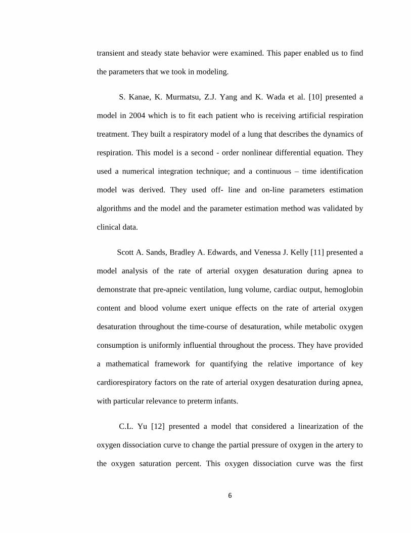
transient and steady state behavior were examined. This paper enabled us to find
the parameters that we took in modeling.
S. Kanae, K. Murmatsu, Z.J. Yang and K. Wada et al. [10] presented a
model in 2004 which is to fit each patient who is receiving artificial respiration
treatment. They built a respiratory model of a lung that describes the dynamics of
respiration. This model is a second - order nonlinear differential equation. They
used a numerical integration technique; and a continuous – time identification
model was derived. They used off- line and on-line parameters estimation
algorithms and the model and the parameter estimation method was validated by
clinical data.
Scott A. Sands, Bradley A. Edwards, and Venessa J. Kelly [11] presented a
model analysis of the rate of arterial oxygen desaturation during apnea to
demonstrate that pre-apneic ventilation, lung volume, cardiac output, hemoglobin
content and blood volume exert unique effects on the rate of arterial oxygen
desaturation throughout the time-course of desaturation, while metabolic oxygen
consumption is uniformly influential throughout the process. They have provided
a mathematical framework for quantifying the relative importance of key
cardiorespiratory factors on the rate of arterial oxygen desaturation during apnea,
with particular relevance to preterm infants.
C.L. Yu [12] presented a model that considered a linearization of the
oxygen dissociation curve to change the partial pressure of oxygen in the artery to
the oxygen saturation percent. This oxygen dissociation curve was the first

7
proposed by Severinghaus, and it is used to convert partial pressure of oxygen to
oxygen saturation in blood. This paper was very important for us to help us to
create the modeling of the efficient controller for Arterial Saturation in Infants.
They informed us above the ways to study the compartments work and how we
can make the equation of modeling, how we can use the Oxygen Saturation curve
and the limit of 𝑆𝑝𝑂2with changing in values of 𝑃𝑎𝑂2.
We took these results in the creation of our modeling.
8
1.2.2 Review of Control Systems
There are many control systems that have been presented in the literature.
L. Zhang, and R.G. Cameron proposed a real – time rule-based control strategy
for blood gas regulation of preterm infants under ventilation treatment [13]. The
General Predictive Control (GPC) controller was investigated using computer
simulation. They used a first - order autoregressive–moving-average (ARMA)
model to represent the respiratory system and Recursive Least Square (RLS)
estimation algorithm to cope with nonlinearity and time varying characteristics of
the system. Based on the results of the simulation and support from experienced
pediatritions, the scheme is very promising for clinical applications. They chose
GPC to control the partial pressure ( 𝑃𝑎𝑂2) and ( 𝑃𝑎𝐶𝑂2
) by adjusting the
concentration of oxygen ( 𝐹𝑖𝑂2) in the air they inspire. The results of the
simulation were very encouraging from the expert system for a set of ventilator
adjustments. From this paper we learned what the effect is of constraints on the
GPC to make decisions for changing 𝐹𝑖𝑂2 levels.
In 1991 Tehrani et al. proposed a PID controller using a feedback signal of
arterial oxygen saturation of the premature infant. It was used to adjust the
concentration of inspired oxygen under the incubator [14]. They used a computer
simulation, and the performance of the control system was evaluated under
different test conditions to investigate the performance of the control system. The
concentration of oxygen in the inspired gas (𝐹𝑖𝑂2) of the neonate was adjusted to
provide for sufficient oxygenation of the blood and was low enough to prevent the
damaging effects of oxygen toxicity. They calculated the values of parameters of

9
a PID controller after a number of preliminary simulation experiments. The effect
of the PID controller on the system is to make arterial pressure reach the set point
with in a small time period. The results were stable and indicative of the
effectiveness of the controller under two different tests.
In 1991 John Taube M.S. and Vinod Bhutani M.D. et al. proposed a computer
simulation with PID controller between the oxygen sensing and an oxygen
blender for premature infants in [15]. They used a closed loop oxygen controller
for the automatic control of supplemental oxygen because the regulation in open
loop is a mismatch between the supplemental oxygen provided and the needs of
the patient. PID controller software program was used to calculate a signal to the
control oxygen blender output by using hemoglobin saturation (HSAT) from a
pulse oximeter as feedback. It produced a fast response of hemoglobin saturation
with little overshoot and gave a desired steady state error. The automatic control
of oxygen was a more accurate method of regulating the blood oxygen level in the
premature infants.
C. Yu, W. He, J. So, R. Roy and H. Kaufman. et al proposed to use a multiple
– model adaptive controller (MMAC) for regulating oxygen saturation with
changing input 𝐹𝑖𝑂2 [16]. The procedure in MMAC assumes that the system can
be represented by one of a finite number of models and used to desensitize the
system to gain variation. Computer-based proportional – integral (PI) simulations
demonstrated the effectiveness of the algorithm over a wide variation of plant
parameters. The fixed PI controller was designed to give no steady state error and
the simulation showed that variations in plant parameters did not adversely affect
10
the transient response. The controller was commanded to raise 𝑆𝑎𝑂2 from an
initial value of about 80% to a reference level of 95% and to maintain it at the
new set point and by changing the values of gain, time constant and dead space
time for plant at constant sampling period. Atypical step response illustration
𝑆𝑎𝑂2 changes, 𝐹𝑖𝑂2 level and the weights for each model. Results of both
simulations and animal experiments demonstrate the ability of the MMAC
controller to effectively regulate 𝑆𝑎𝑂2 despite the presence of system
disturbances.
Paul E. Morozoff, Ron W. Evans and John A. Smyth et al proposed an
automatic control to regulate blood oxygen saturation [17]. The automatic 𝑆𝑎𝑂2
controller was constructed to assist clinical staff in improving a premature infant’s
condition by reducing the duration and frequency of hypoxemic and hyperoxemic
episodes. They used a control algorithm based on the sign of the error magnitude,
velocity and acceleration as input and then applied these inputs to a state machine
to determine the trend of the error. Error is defined as the observed oxygen
saturation minus the target oxygen saturation. The feature of this algorithm was
that it could accommodate the non-linearity of the system. Each of the state
machines can provide 𝐹𝑖𝑂2 adjustment and delay times, and the state machine
was built to identify trends of 𝑆𝑎𝑂2 moving towards or away from the target. A
single set of machine parameters was used by the controller to regulate the
oxygen saturation with eight infants in the clinical trials. During this study a
generic set of state machine 𝐹𝑖𝑂2 increments, decrements and delay time was
determined. They found that with large variability of physiology and 𝑆𝑎𝑂2
11
stability between neonates, a single set of state machine parameters could be used by
the controller to regulate a patient’s𝑆𝑎𝑂2. They found that if 𝑆𝑎𝑂2 dropped suddenly
as result of shunting, the controller could not react fast enough and that required
the manual intervention as signaled by the controller’s 𝑆𝑎𝑂2 limiting. Results
from this paper proved that the automatic control systems are becoming more
prevalent and increased the duration that the neonate spent at normal 𝑆𝑎𝑂2 and the
number of manual interventions required by clinical staff.
Keim proposed to design single robust controller based on a linear model of
premature infants [18]. The robust controller was designed based on an error
model and performance specifications. He developed an adaptive controller
based on estimated parameters and disturbances. The controller regulated the
𝐹𝑖𝑂2 while mitigating disturbances. The 𝐻∞ is used in control theory to
synthesize controllers achieving robust performance or stabilization. The 𝐻∞ is
used for plants having problems involving multivariable systems. In this paper, a
performance requirement is developed in the frequency domain for the purpose of
control design and analysis. To check for performance, the following inequality
must hold for all frequencies,
‖𝑁22‖∞ ≤ 1
where ‖𝑁22‖∞ is a frequency domain performance measure.
The plot of the 𝐻∞ norm of 𝑁22 was always less than one, so the system has
nominal performance. The control signals for adaptive and 𝐻∞ control systems
have saturation limits such that the signals do not go below 0%, since that level is
12
considered to be equal to room air. The adaptive control system is able to reject
the disturbances and has 0% overshoot. The 𝑆𝑝𝑂2 from the closed loop control
simulation did not drop beneath 2% due to the disturbances. The robust control
system has slow performance due to the low bandwidth frequency that is used for
control design. The robust control system also has 0% overshoot. The control
signal for the adaptive controller is smaller than that of the robust controller. For
these reasons, the robust control is better than the adaptive control.
Deacha C., Anan W., and Kitiphol C. proposed to design an automatic
control for oxygen intake via nasal cannula in premature infants [19]. They used a
new computer - based system combining to the nasal cannula for automatically
controlling the quantity of oxygen intake. A pulse oximeter is currently used in
clinical settings for noninvasive and continuous monitoring of arterial oxygen in
infants. In flow control of oxygen, commands are transferred from a computer
into the data acquisition (DAC) interface by USB port. Then it sends digital data
to drive a stepping motor for speed control. The performance of the system was
evaluated by operating with a 𝑆𝑝𝑂2 simulator showing satisfactory results with
low tracking error. The computer controlled the natal cannula 𝐹𝑖𝑂2 flow by
using a pulse oximeter as indicator for arterial oxygen saturation in blood ( 𝑆𝑎𝑂2)
in the feedback loop control, oxygen intake needed, calculated from the model is
fed via controlled values. The process operates on a microcomputer programmed
on the national Instruments LabView(R).
Nelson C., Tilo G., Ruth E., Gabriel M., Carmen H., and Edua proposed an
algorithm for closed-loop inspired oxygen control for mechanical ventilation [20].
13
They developed an algorithm to maintain 𝑆𝑝𝑂2 within a target range. The closed
– loop control was compared with continuous manual 𝐹𝑖𝑂2 adjustments by a
nurse with a group of ventilated infants who presented with frequent episodes of
hypoxemia. There were two 𝐹𝑖𝑂2 control modes : the 𝑐𝐹𝑖𝑂2 algorithm defines
𝑆𝑝𝑂2 ranges based on a user - defined target range of normal blood levels of
oxygen (normoxemia); the 𝑚𝐹𝑖𝑂2 was the reference mode to which the 𝑐𝐹𝑖𝑂2
algorithm was compared consisted of manual adjustments of the 𝐹𝑖𝑂2 made
continuously by a neonatal research nurse station, fully dedicated to maintain
𝑆𝑝𝑂2 within the same target range of (normoxemia) . Computerized analysis was
used to calculate mean 𝑆𝑝𝑂2, frequency and duration of episodes of hypoxemia.
They selected fourteen very low birth weight (VLBW) infants undergoing
mechanical ventilation which were included in this study. Although it remains to
be proven, they speculated that long-term closed – loop 𝐹𝑖𝑂2 control may reduce
nursing time spent to maintain adequate oxygenation and reduce the risk of
morbidity associated with supplemental oxygen.
1.2.3 Review of PI Controllers
Proportional Integral (PI) Controllers have been used in industry with
linear and nonlinear systems. S. Anand, Aswin. V., and S. Rakesh kumar showed
in 2011 a design continuously tuned adaptive PI controller for a non-linear
process as a conical tank [21]. A simple tuning system was used to continuously
tune the controller parameters in correspondence with the change in operating
14
points. The tuning system had the ability to interpolate and extrapolate the
relationship between the control variable and the controller parameters over entire
span of control variables. Then the PI controller was able to produce minimum
overshoots and minimum settling time. Rubiyah and Sigeru in 1994 used the PI
controller to the temperature controlled water bath [22]. It has ability of the
controllers to handle process with variable time delays. Tunyasrirut and
Ngamwiwit in 1999 presented a design of adaptive PI controller to control the
speed of separately excited DC motor by self – tuning [23]. The designed
controller to control the armature voltage while the field voltage was fixed as a
constant. F.T. Tehrani in 2001 designed control system was proposed for oxygen
therapy for premature infants [24]. The control software is used as well as a PI
control algorithm to provide fast and efficient response to changes in arterial
oxygen saturation of the infant detected by pulse oximetery.
1.2.4. Review of PID Controllers
PID Control systems have been used with many industrial devices. Noor and
Mahanijah in 2009 presented the comparison of performance between a PID
temperature controller and a conventional on-off temperature controller for a
home – applied refrigerator [25]. They designed PID and evaluated it using
MATLAB Simulink software. They found that the proposed PID temperature
controller performed better than the on-off controller in maintaining the set value
15
of the system which is the inner temperature of the refrigerator and PID controller
was working more efficiently to maintain the inner temperature of the refrigerator
than the on-off controller. M.H. Moradi in 2003 presented to design of predictive
PID controllers [26]. He proposed that a controller can deal with future set points
and the process dead time can be incorporated without any need for
approximation. He found that the main advantages of the proposed controller
were that it can be used with systems of any order and the PID tuning can be used
to adjust the controller performance. Arulmozhiyal and Kandiban in 2012
proposed an improved PID controller to control speed of brushes DC motor [27].
They presented simulation results of conventional PID controller and Fuzzy PID
controller of the three brushless DC motor. They found that the Fuzzy controller
showed better performance than PID controller at lower and high speeds. Taube
and Pillutla in 1988 developed with another colleague for closed loop
supplemental oxygen treatment of newborn [28]. They used PID control design
for an adaptive control system to maintain blood oxygen levels at desired levels.
This design was clearly usable in an intensive care nursery environment.
1.2.5. Review of Model Predictive Controller (MPC)
Model Predictive Control (MPC) has been used in the academic and
industrial studies. Alicia and Alejandro in 2010 proposed two controls to manage
the air supply of the fuel-cell system [29]. They improved transient responses and
better fuel-cell efficiency in the case of the efficiency maximization objective.

16
C. Yu and W. He proposed a computer – based proportional – integral (PI)
controller has been developed to control arterial oxygen levels in mechanically –
ventilated animals [16]. They designed a multiple model adaptive control
(MMPC) to desensitize the system to these gain variables and compared it with
the PI controller.
1.2.6. Review of Robustness Analysis
Very little work has been done to analyze the robustness of controllers for an
oxygen saturation control system. In 2001 Tehrani showed robustness by testing
the control system for two different desaturation periods [23]. The model range of
parameters for testing the robustness of the controller was not large enough and
no techniques such as H-infinity robustness analysis were used to show that the
control systems guaranteed robust performance and stability. Keim proposed a
controller to control arterial oxygen saturation in neonatal infants [18]. Krone
also proposed a robust controller to reject the disturbances caused by variations in
Heart Rate (HR) and Respiratory Rate (RR) to keep the 𝑆𝑝𝑂2 at given set point
[30]. Keim developed a single robust controller based on a linear model. The
robust controller was designed based on an error model and performance
specifications. Keim developed an adaptive controller based on estimate
parameters and disturbances. The controller attempted to regulate the 𝐹𝑖𝑂2 while
mitigate the affect of the disturbances. Krone designed a robust controller with
an average 𝑆𝑝𝑂2 of 6.623e-004% and a maximum 𝑆𝑝𝑂2 value of 0.0725%. The
17
𝑆𝑝𝑂2 was normalized at 90% and the 𝐹𝑖𝑂2 was normalized at 21%. The 𝑆𝑝𝑂2
and 𝐹𝑖𝑂2 values presented were the difference between the actual values and the
nominal values.
1.3. Overview of Following Chapters
In Chapter 2, the respiratory system model by Yu will be used to
analyze the model after desaturation periods. We have chosen this model
because it has one input that is 𝐹𝑖𝑂2 and one output that is 𝑆𝑝𝑂2. This model
was relinearized to find a linear model at the operating point. Data from
Columbia Regional Hospital now known as the University of Missouri
Women’s and Children’s Hospital will be discussed and used to compare and
will use Yu’s model. In Chapter 3, we designed PI, PID, and MPC for the
systems. A digital PI and PID controller designed to control 𝐹𝑖𝑂2 to get the
range values of 𝑆𝑝𝑂2 between 85% to 92% with minimum overshoot and
zero steady state error. A model Predictive Control (MPC) was designed to
predict 𝑆𝑝𝑂2 by finding the best values of control horizon and moving
horizon. The most important part of strategy was obtaining the control law.
With the control law found, the values of 𝐹𝑖𝑂2 were determined that control
the plant to get good response without peak overshoot and zero error steady
state. In Chapter 4, a robust analysis of the system is performed and a robust
controller is developed. The range of system gains and time constants used in
the analysis are taken from Krone’s thesis [30]. It is shown that a single,

18
static controller can guarantee robust performance for all the ranges of
parameters. In Chapter 5, an overview of the construction of the whole
system with designing controller of an oxygen control prototype is presented.
We suggest conclusions and a plan for future work.
19
Chapter 2: Methodology: Modeling the Respiratory System Model
2.1. Overview of the Respiratory System Model
We used model that is based on prior research completed by Yu. This model
was a nonlinear model to describe the relationship between 𝑆𝑝𝑂2 with the
input 𝐹𝑖𝑂2. In this investigation, we took modeling by Yu with the effect of
heart rate (HR) and respiratory rate (RR) as disturbances.
There are two major parts in the respiratory system: the lungs and the
circulating blood that transports the oxygen to the other part of the human body.
In the lungs, there are three compartments. The first compartment of the lung with
volume, 𝑉𝐴, is perfused with blood flow, 𝑄𝑝 , and is ventilated with a respiratory
rate of �̇�𝐴. The second lung compartment corresponds to the dead zone in the
lung. All dead zone in the lung is lumped into one parameter called the dead zone
ratio, 𝑥𝑑. The ventilation to the first lung volume can be define as
𝑉�̇� = ( 1 − 𝑥𝑑) �̇�𝐼̇ (2.1)
where �̇�𝐼 is the total respiratory rate. The third lung compartment is perfused with
blood. It introduces a shunt ratio, 𝑦𝑠. The ratio will affect how much blood flow
will reach the first lung compartment by
𝑄𝑝 = (1 − 𝑦𝑠)𝑄 (2.2)
20
where Q is the total blood flow to the respiratory system. We took linear and
nonlinear models with the assumption that all flow is constant and unidirectional.
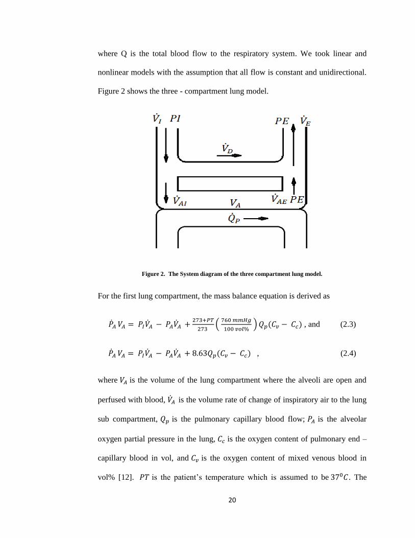
Figure 2 shows the three - compartment lung model.
Figure 2. The System diagram of the three compartment lung model.
For the first lung compartment, the mass balance equation is derived as
�̇�𝐴 𝑉𝐴 = 𝑃𝐼�̇�𝐴 − 𝑃𝐴�̇�𝐴 +273+𝑃𝑇
273 (
760 𝑚𝑚𝐻𝑔
100 𝑣𝑜𝑙% ) 𝑄𝑝(𝐶𝑣 − 𝐶𝑐) , and (2.3)
�̇�𝐴 𝑉𝐴 = 𝑃𝐼�̇�𝐴 − 𝑃𝐴�̇�𝐴 + 8.63𝑄𝑝(𝐶𝑣 − 𝐶𝑐) , (2.4)
where 𝑉𝐴 is the volume of the lung compartment where the alveoli are open and
perfused with blood, �̇�𝐴 is the volume rate of change of inspiratory air to the lung
sub compartment, 𝑄𝑝 is the pulmonary capillary blood flow; 𝑃𝐴 is the alveolar
oxygen partial pressure in the lung, 𝐶𝑐 is the oxygen content of pulmonary end –
capillary blood in vol, and 𝐶𝑣 is the oxygen content of mixed venous blood in
vol% [12]. 𝑃𝑇 is the patient’s temperature which is assumed to be 370𝐶. The
21
constant 8.63 is a factor to convert gas concentrations and saturated and saturated
water vapor conditions to temperature and pressure under normal body
conditions.
By taking a first – order Taylor series expansion to linearization the mass
balance nonlinear differential nonlinear equation in the work by Yu is given as
�̇�𝐴 𝑉𝐴 = �̇�𝐴 𝑉𝑜,𝐴 + ∆�̇�𝐴 𝑉𝐴 .
𝑃𝐼�̇�𝐴 = 𝑃𝑜,𝐼�̇�𝐴 + 𝑃𝐼∆�̇�𝐴 .
𝑃𝐴�̇�𝐴 = 𝑃𝑜,𝐴�̇�𝐴 + 𝑃𝐴∆�̇�𝐴. (2.5)
𝐶𝑣 = 𝐶𝑜,𝑣 + 𝛽𝑣∆𝑃𝑣.
𝐶𝑐 = 𝐶𝑜,𝑐 + 𝛽𝑐∆𝑃𝐴.
�̇�𝐴 𝑉𝑜,𝐴 + ∆�̇�𝐴 𝑉𝐴 = 𝑃𝑜,𝐼�̇�𝐴 + 𝑃𝐼∆�̇�𝐴 – 𝑃𝑜,𝐴�̇�𝐴 − 𝑃𝐴∆�̇�𝐴 + 8.63𝑄𝑝((𝐶𝑜,𝑣 +
𝛽𝑣∆𝑃𝑣) − (𝐶𝑜,𝑐 + 𝛽𝑐∆𝑃𝐴)). (2.6)
With initial value is zero we get
∆�̇�𝐴 𝑉𝐴 = 𝑃𝐼∆�̇�𝐴 − 𝑃𝐼∆�̇�𝐴 + 8.63𝑄𝑝( 𝛽𝑣∆𝑃𝑣 − 𝛽𝑐∆𝑃𝐴) . (2.7)
Where 𝑃𝑣 is the partial pressure of oxygen in the venous blood and is assumed
equal to the partial pressure in the tissue compartment, 𝑃𝑇 . By substituting Eq
(2.1) and (2.2) in (2.7) and get
22
∆�̇�𝐴 𝑉𝐴 = ( 1 − 𝑥𝑑) �̇�𝐼 ∆𝑃𝐼 − ∆𝑃𝐴( 1 − 𝑥𝑑) + 8.63 (1 − 𝑦𝑠)𝑄 ( 𝛽𝑣∆𝑃𝑣 −
𝛽𝑐∆𝑃𝐴). (2.8)
∆�̇�𝐴 𝑉𝐴 = ( 1 − 𝑥𝑑) �̇�𝐼 (∆𝑃𝐼 − ∆𝑃𝐴) + 8.63 (1 − 𝑦𝑠)𝑄 ( 𝛽𝑣∆𝑃𝑇 − 𝛽𝑐∆𝑃𝐴).
(2.9)
It is shown that the system can be modeled in as an open – loop system without
the feedback of the partial pressure of oxygen in the tissue as was done by Yu
[12]. This assumption eliminates the ∆𝑃𝑇 term from Eq (2.9) and gets
∆�̇�𝐴 𝑉𝐴 = ( 1 − 𝑥𝑑) �̇�𝐼 (∆𝑃𝐼 − ∆𝑃𝐴) − 8.63 (1 − 𝑦𝑠)𝑄 𝛽𝑐∆𝑃𝐴.
(2.10)
At the steady state space gain that leads that term in the left side will be zero and
after that we get
( 1 − 𝑥𝑑) �̇�𝐼 (∆𝑃𝐼 − ∆𝑃𝐴) = 8.63 (1 − 𝑦𝑠)𝑄 𝛽𝑐∆𝑃𝐴.
(2.11)
( 1 − 𝑥𝑑) �̇�𝐼 ∆𝑃𝐼 − ( 1 − 𝑥𝑑) �̇�𝐼∆𝑃𝐴 = 8.63 (1 − 𝑦𝑠)𝑄 𝛽𝑐∆𝑃𝐴.
(2.12)
( 1 − 𝑥𝑑) �̇�𝐼 ∆𝑃𝐼 = ( 1 − 𝑥𝑑) �̇�𝐼∆𝑃𝐴 + 8.63 (1 − 𝑦𝑠)𝑄 𝛽𝑐∆𝑃𝐴.
(2.13)
By finding the ratio between ∆𝑃𝐴 to ∆𝑃𝐼 we get
23
∆𝑃𝐴
∆𝑃𝐼=
( 1−𝑥𝑑 ) �̇�𝐼
8.63 (1−𝑦𝑠)𝑄 𝛽𝑐+( 1− 𝑥𝑑) �̇�𝐼 . (2.14)
The variation in 𝑃𝑎 per unit change in alveolar oxygen over a variation in the
oxygen content due to the intrapulmonary shunt is
∆𝑃𝑎
∆𝑃𝐴=
(1−𝑦𝑠)𝛽𝑐
𝛽𝑎. (2.15)
The fractional composition of a gas is related to its partial pressure as
∆𝑃𝐼
∆𝐹𝐼 = 𝑃𝐵 − 𝑃𝐻2𝑜 (2.16)
where 𝑃𝐻2𝑜 is water vapor pressure and 𝑃𝐵 is the barometric pressure. We can get
the steady state gain is
𝐺𝑝 = ∆𝑃𝐴
∆𝑃𝐼 ∆𝑃𝑎
∆𝑃𝐴 ∆𝑃𝐼
∆𝐹𝐼=
( 1−𝑥𝑑 ) �̇�𝐼
8.63 (1−𝑦𝑠)𝑄 𝛽𝑐+( 1− 𝑥𝑑) �̇�𝐼 (1−𝑦𝑠)𝛽𝑐
𝛽𝑎 (𝑃𝐵 − 𝑃𝐻2𝑜).
(2.17)
Where the parameter 𝛽𝑎 is the equivalent to the slope of the tangent line of the
oxygen dissociation curve at the current partial pressure of oxygen in artery.
from Eq (10) can we get the homogenous equation as
𝑉𝐴
[(1−𝑥𝑑) �̇�𝐼+8.63 (1−𝑦𝑠)𝑄 𝛽𝑐] ∆�̇�𝐴 + ∆𝑃𝐴 = 0. (2.18)
Where the parameter 𝛽𝑐 is the apparent solubility of oxygen in whole blood in the
alveolar. From Eq (10) a time constant for the lung can be
𝜏 = 𝑉𝐴
8.63 (1−𝑦𝑠)�̇�𝑃 𝛽𝑐+( 1− 𝑥𝑑) �̇�𝐼=
𝑉𝐴
�̇�𝐴+ 8.63 �̇�𝑃 𝛽𝑐. (2.19)
24
We can find the time constant at nominal condition when using nominal system
parameters.
A linearized model of the respiratory system of neonatal infants is derived as
𝜏∆𝑃𝑎𝑠 + ∆𝑃𝑎 = 𝐺𝑝∆𝐹𝑖𝑜2. (2.20)
Where 𝐺𝑝 is the steady state system gain, ∆𝑃𝑎 is the linearized partial pressure of
oxygen in the lung. The parameters for the linear system are computed at nominal
conditions. To modify the system such that the output is 𝑂2 , the oxygen
dissociation curve that was derived by Severinghaus is evaluated at the partial
pressure of oxygen in the artery, 𝑃𝑎 [11]. The oxygen dissociation curve is defined
by
𝑆𝑝𝑂2 = 1
23400[𝑃𝑎 3+150𝑃𝑎]−1+1
(100%). (2.21)
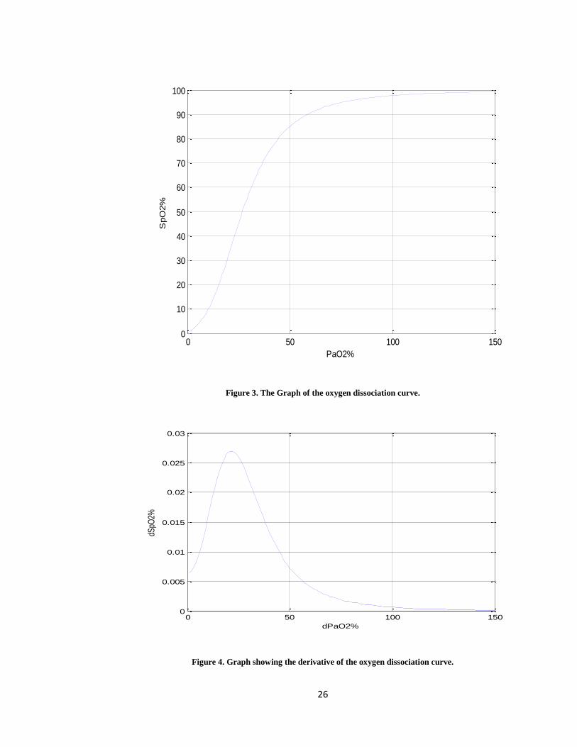
The curve of the oxygen dissociation can be seen in Figure 2. The derivative of
equation (2.21) with respect to 𝑃𝑎 is computed at nominal conditions curve gain,
𝐺𝑐, is used to convert 𝑃𝑎 to 𝑆𝑝𝑂2 by
∆𝑆𝑝𝑂2 = 𝐺𝑐∆𝑃𝑎𝑂.2
∆𝑆�̇�𝑂2 = 𝐺𝑐∆�̇�𝑎𝑂2. (2.22)
From Eq (2.22) we can get ∆𝑃𝑎𝑂2 as
∆𝑃𝑎𝑂2 = ∆𝑆𝑝𝑂2
𝐺𝑐. (2.23)
By substitution equation from (2.23) in (2.20) and get
25
𝜏∆𝑆𝑝𝑂2
𝐺𝑐 𝑠 +
∆𝑆𝑝𝑂2
𝐺𝑐= 𝐺𝑝∆𝐹𝑖𝑜2. (2.24)
𝜏 ∆𝑆𝑝𝑂2 𝑠 + ∆𝑆𝑝𝑂2 = 𝐺𝑝 𝐺𝑐 ∆𝐹𝑖𝑜2. (2.25)
𝜏 ∆𝑆𝑝𝑂2 𝑠 + ∆𝑆𝑝𝑂2 = 𝐺𝑝𝑐 ∆𝐹𝑖𝑜2. (2.26)
𝐺𝑝𝑐 = 𝐺𝑝 𝐺𝑐 . (2.27)
We can solve 𝛽 parameters from the derivation of the oxygen dissociation curve
and is evaluated for the range of partial pressure of oxygen and is given by the
equation
𝑑𝑠𝑝𝑂2
𝑑𝑃𝑎=
23400(3𝑃𝑎2+150)
(𝑃𝑎3+150𝑃𝑎)2(
23400
𝑃𝑎3+150𝑃𝑎
+1)2. (2.28)
In Figure 3, we can show the graph of the derivative of the oxygen dissociation
curve. In the alveolar capillary that the partial pressure of oxygen is not known
from this model and is solved for based on the output 𝑃𝑎. The alveolar capillary
partial pressure is solved for using
𝑃𝐴𝑂2 = 𝑃𝑎𝑂2 + 𝐾𝑎. (2.29)
where 𝐾𝑎 is the alveolar – arterial oxygen difference [9]. The alveolar – arterial
oxygen difference is assumed to be 1.5% which is the nominal difference between
the two saturations. By using Eq (2.27) and the oxygen dissociation curve, the
alveolar capillary partial pressure can be determined.
26
Figure 3. The Graph of the oxygen dissociation curve.
Figure 4. Graph showing the derivative of the oxygen dissociation curve.
0 50 100 1500
10
20
30
40
50
60
70
80
90
100
PaO2%
SpO
2%
0 50 100 1500
0.005
0.01
0.015
0.02
0.025
0.03
dSpO
2%
dPaO2%
27
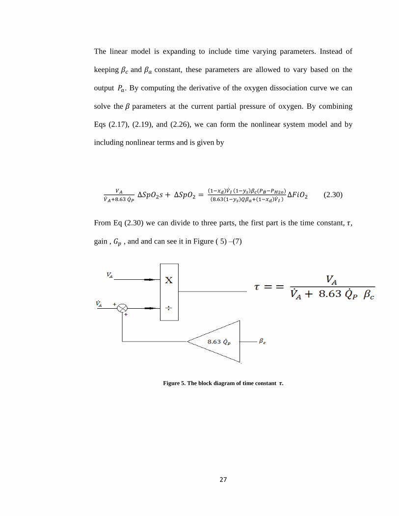
The linear model is expanding to include time varying parameters. Instead of
keeping 𝛽𝑐 and 𝛽𝑎 constant, these parameters are allowed to vary based on the
output 𝑃𝑎. By computing the derivative of the oxygen dissociation curve we can
solve the 𝛽 parameters at the current partial pressure of oxygen. By combining
Eqs (2.17), (2.19), and (2.26), we can form the nonlinear system model and by
including nonlinear terms and is given by
𝑉𝐴
�̇�𝐴+8.63 �̇�𝑃 ∆𝑆𝑝𝑂2𝑠 + ∆𝑆𝑝𝑂2 =
(1−𝑥𝑑)�̇�𝐼 (1−𝑦𝑠)𝛽𝑐(𝑃𝐵−𝑃𝐻2𝑜)
(8.63(1−𝑦𝑠)𝑄𝛽𝑎+(1−𝑥𝑑)�̇�𝐼 )∆𝐹𝑖𝑂2 (2.30)
From Eq (2.30) we can divide to three parts, the first part is the time constant, 𝜏,
gain , 𝐺𝑝 , and and can see it in Figure ( 5) –(7)
Figure 5. The block diagram of time constant 𝝉.
28
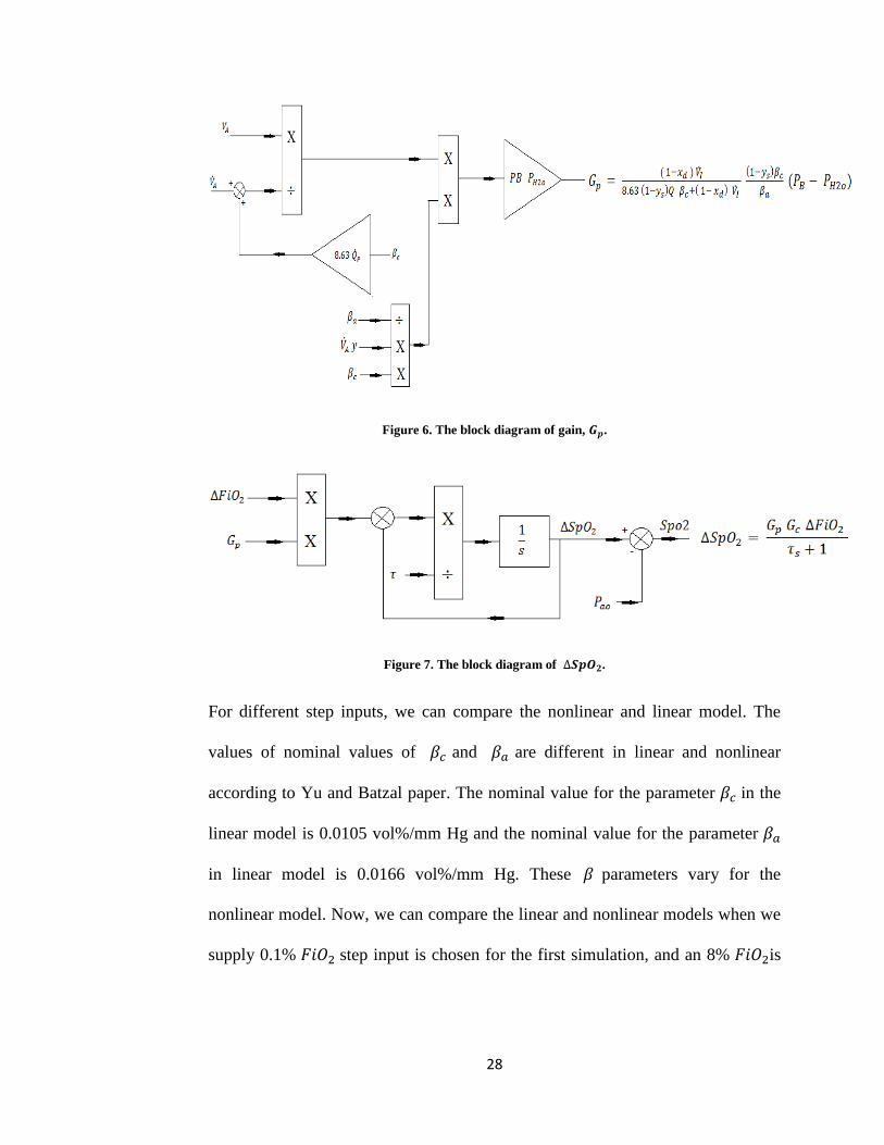
Figure 6. The block diagram of gain, 𝑮𝒑.
Figure 7. The block diagram of ∆𝑺𝒑𝑶𝟐.
For different step inputs, we can compare the nonlinear and linear model. The
values of nominal values of 𝛽𝑐 and 𝛽𝑎 are different in linear and nonlinear
according to Yu and Batzal paper. The nominal value for the parameter 𝛽𝑐 in the
linear model is 0.0105 vol%/mm Hg and the nominal value for the parameter 𝛽𝑎
in linear model is 0.0166 vol%/mm Hg. These 𝛽 parameters vary for the
nonlinear model. Now, we can compare the linear and nonlinear models when we
supply 0.1% 𝐹𝑖𝑂2 step input is chosen for the first simulation, and an 8% 𝐹𝑖𝑂2is
29
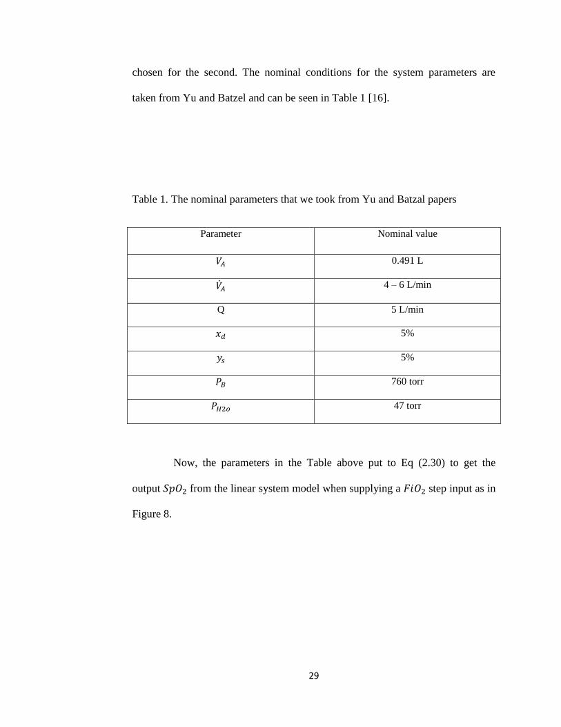
chosen for the second. The nominal conditions for the system parameters are
taken from Yu and Batzel and can be seen in Table 1 [16].
Table 1. The nominal parameters that we took from Yu and Batzal papers
Parameter Nominal value
𝑉𝐴 0.491 L
�̇�𝐴 4 – 6 L/min
Q 5 L/min
𝑥𝑑 5%
𝑦𝑠 5%
𝑃𝐵 760 torr
𝑃𝐻2𝑜 47 torr
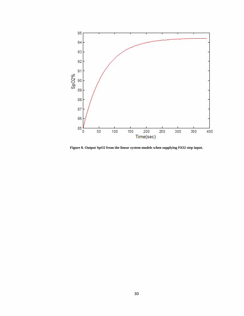
Now, the parameters in the Table above put to Eq (2.30) to get the
output 𝑆𝑝𝑂2 from the linear system model when supplying a 𝐹𝑖𝑂2 step input as in
Figure 8.
30
Figure 8. Output SpO2 from the linear system models when supplying FiO2 step input.
31
Chapter 3: Controller of the System
This chapter describes three controller methods; Proportional – integral
(PI), Proportional – Integral – Derivative (PID) and Model Predictive Control
(MPC). Theses controllers need algorithms to define how the control action will
affect the behavior of the output response and we derive each controller to be
input 𝐹𝑖𝑂2 to the plant to get output 𝑆𝑝𝑂2.
3.1. Proportional Integral (PI) Controller.
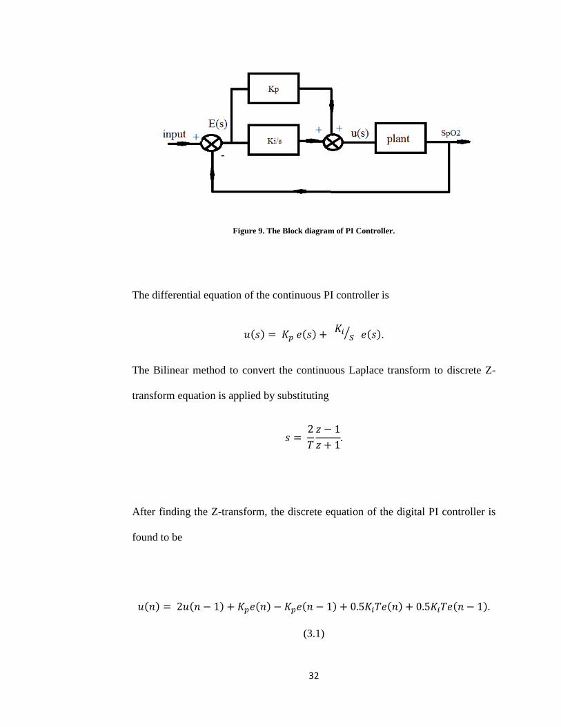
A fixed proportional – integral (PI) controller was connected in feed -
forward to control arterial oxygen saturation 𝑆𝑝𝑂2 by adjusting inspired oxygen
fraction, 𝐹𝑖𝑂2. The performance of the feedback system was found to be sensitive
to the open-loop plant gain. To get an acceptable transient behavior, the controller
was tuned using trial and error selection of 𝐾𝑝 and 𝐾𝑑 in the closed – loop system
as in Fig 9.
32
Figure 9. The Block diagram of PI Controller.
The differential equation of the continuous PI controller is
𝑢(𝑠) = 𝐾𝑝 𝑒(𝑠) + 𝐾𝑖
𝑠⁄ 𝑒(𝑠).
The Bilinear method to convert the continuous Laplace transform to discrete Z-
transform equation is applied by substituting
𝑠 = 2
𝑇
𝑧 − 1
𝑧 + 1.
After finding the Z-transform, the discrete equation of the digital PI controller is
found to be
𝑢(𝑛) = 2𝑢(𝑛 − 1) + 𝐾𝑝𝑒(𝑛) − 𝐾𝑝𝑒(𝑛 − 1) + 0.5𝐾𝑖𝑇𝑒(𝑛) + 0.5𝐾𝑖𝑇𝑒(𝑛 − 1).
(3.1)
33
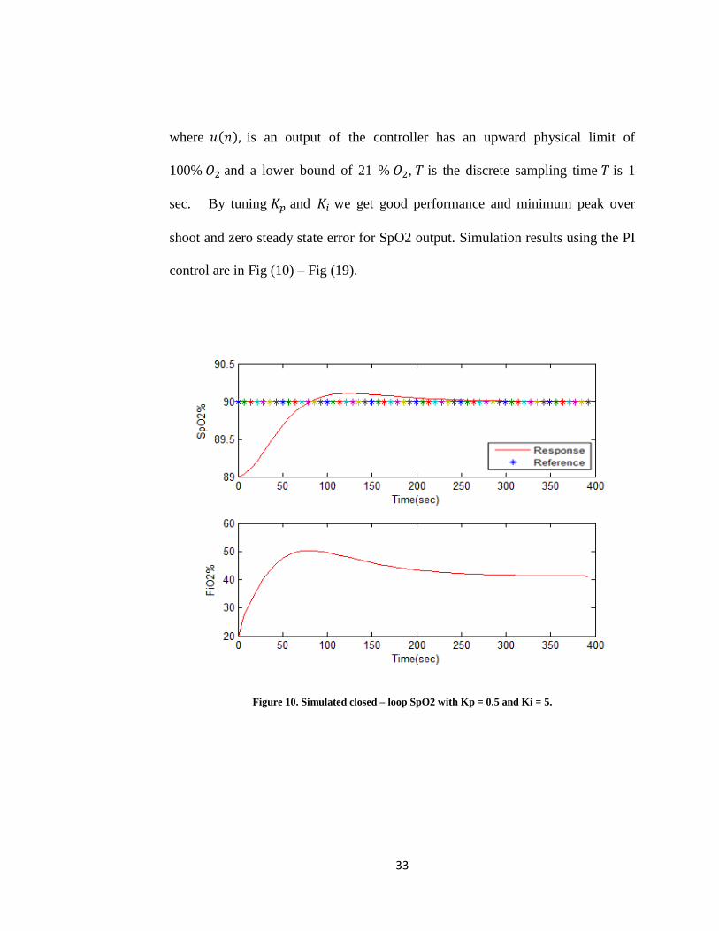
where 𝑢(𝑛), is an output of the controller has an upward physical limit of
100% 𝑂2 and a lower bound of 21 % 𝑂2, 𝑇 is the discrete sampling time 𝑇 is 1
sec. By tuning 𝐾𝑝 and 𝐾𝑖 we get good performance and minimum peak over
shoot and zero steady state error for SpO2 output. Simulation results using the PI
control are in Fig (10) – Fig (19).
Figure 10. Simulated closed – loop SpO2 with Kp = 0.5 and Ki = 5.
34
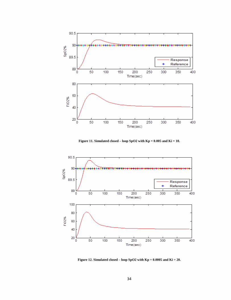
Figure 11. Simulated closed – loop SpO2 with Kp = 0.005 and Ki = 10.
Figure 12. Simulated closed – loop SpO2 with Kp = 0.0005 and Ki = 20.
35
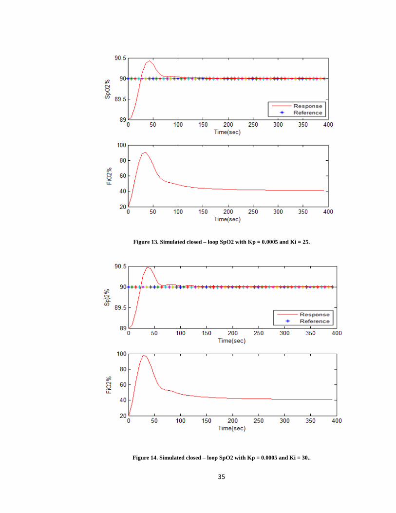
Figure 13. Simulated closed – loop SpO2 with Kp = 0.0005 and Ki = 25.
Figure 14. Simulated closed – loop SpO2 with Kp = 0.0005 and Ki = 30..

36
Figure 15. Simulated closed – loop SpO2 with Kp = 0.0005 and Ki = 40.
Figure 16. Simulated closed – loop SpO2 with Kp = 0.0005 and Ki = 50.
37
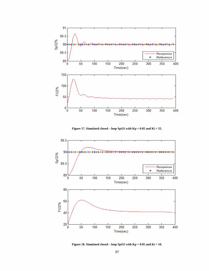
Figure 17. Simulated closed – loop SpO2 with Kp = 0.05 and Ki = 55.
Figure 18. Simulated closed – loop SpO2 with Kp = 0.05 and Ki = 10.
38
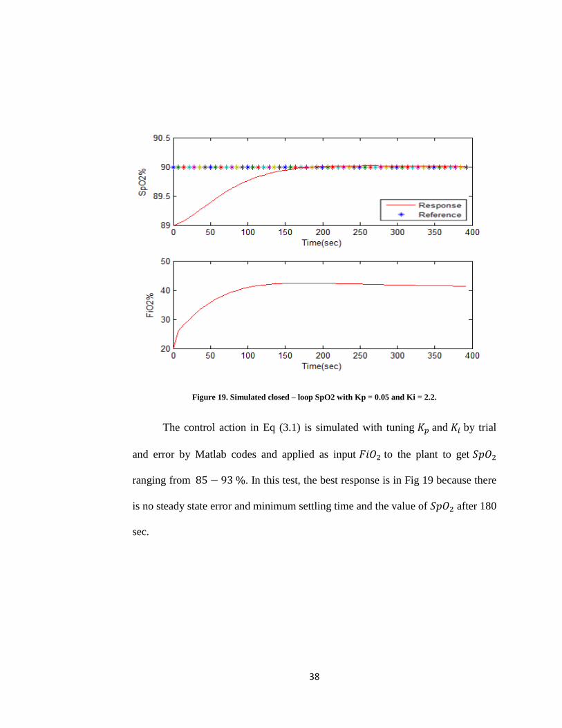
Figure 19. Simulated closed – loop SpO2 with Kp = 0.05 and Ki = 2.2.
The control action in Eq (3.1) is simulated with tuning 𝐾𝑝 and 𝐾𝑖 by trial
and error by Matlab codes and applied as input 𝐹𝑖𝑂2 to the plant to get 𝑆𝑝𝑂2
ranging from 85 − 93 %. In this test, the best response is in Fig 19 because there
is no steady state error and minimum settling time and the value of 𝑆𝑝𝑂2 after 180
sec.
39
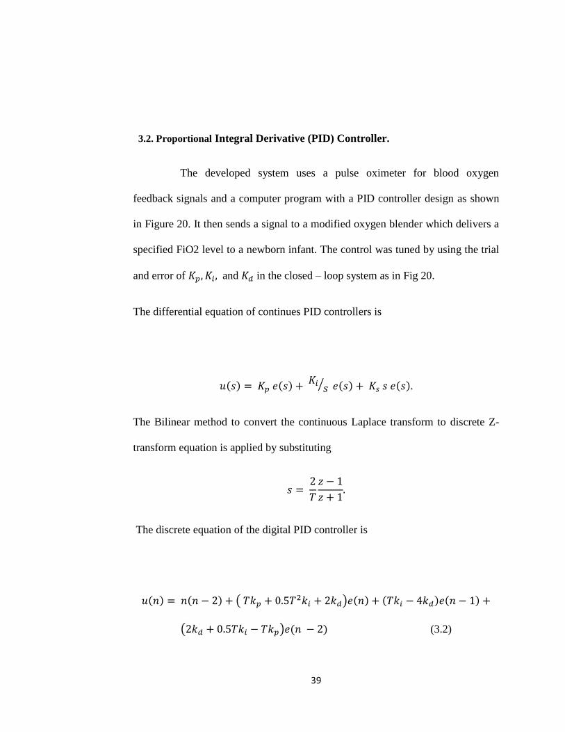
3.2. Proportional Integral Derivative (PID) Controller.
The developed system uses a pulse oximeter for blood oxygen
feedback signals and a computer program with a PID controller design as shown
in Figure 20. It then sends a signal to a modified oxygen blender which delivers a
specified FiO2 level to a newborn infant. The control was tuned by using the trial
and error of 𝐾𝑝, 𝐾𝑖, and 𝐾𝑑 in the closed – loop system as in Fig 20.
The differential equation of continues PID controllers is
𝑢(𝑠) = 𝐾𝑝 𝑒(𝑠) + 𝐾𝑖
𝑠⁄ 𝑒(𝑠) + 𝐾𝑠 𝑠 𝑒(𝑠).
The Bilinear method to convert the continuous Laplace transform to discrete Z-
transform equation is applied by substituting
𝑠 = 2
𝑇
𝑧 − 1
𝑧 + 1.
The discrete equation of the digital PID controller is
𝑢(𝑛) = 𝑛(𝑛 − 2) + ( 𝑇𝑘𝑝 + 0.5𝑇2𝑘𝑖 + 2𝑘𝑑)𝑒(𝑛) + (𝑇𝑘𝑖 − 4𝑘𝑑)𝑒(𝑛 − 1) +
(2𝑘𝑑 + 0.5𝑇𝑘𝑖 − 𝑇𝑘𝑝)𝑒(𝑛 − 2) (3.2)
40
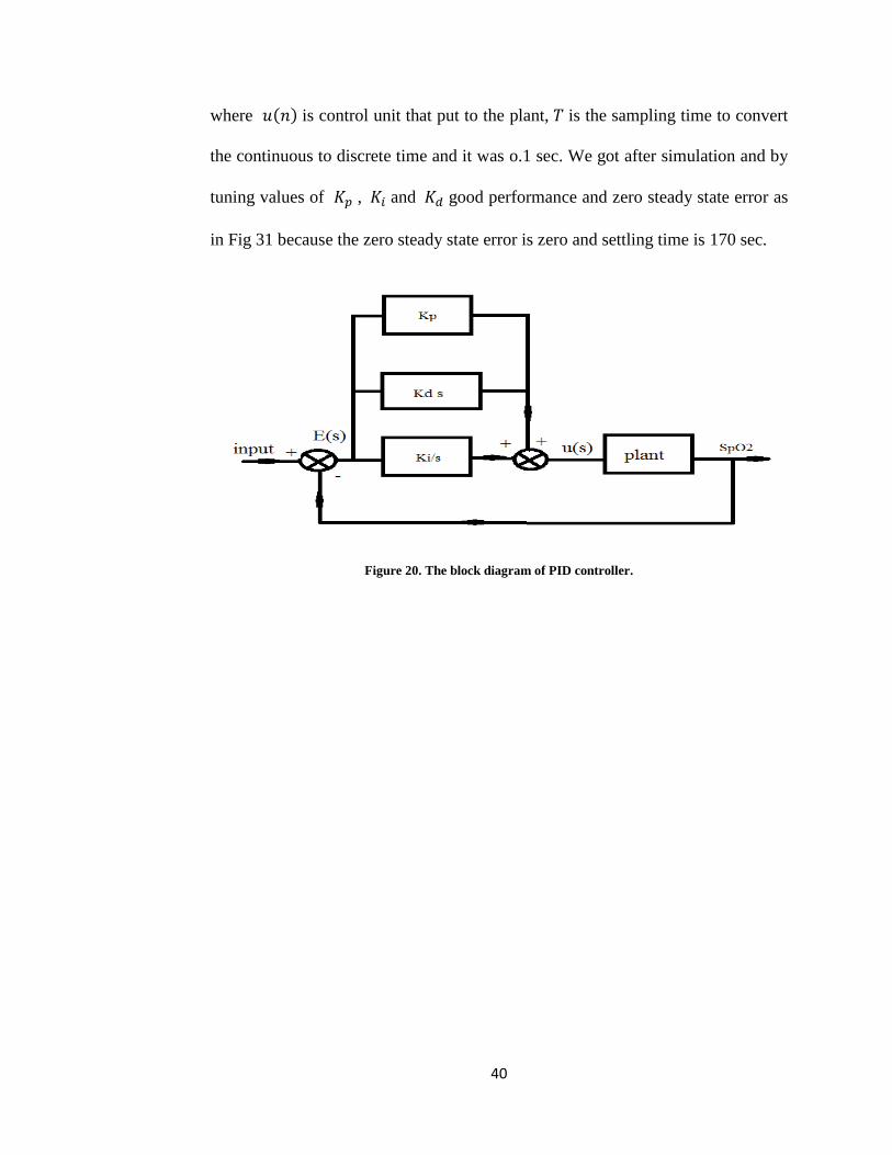
where 𝑢(𝑛) is control unit that put to the plant, 𝑇 is the sampling time to convert
the continuous to discrete time and it was o.1 sec. We got after simulation and by
tuning values of 𝐾𝑝 , 𝐾𝑖 and 𝐾𝑑 good performance and zero steady state error as
in Fig 31 because the zero steady state error is zero and settling time is 170 sec.
Figure 20. The block diagram of PID controller.
41
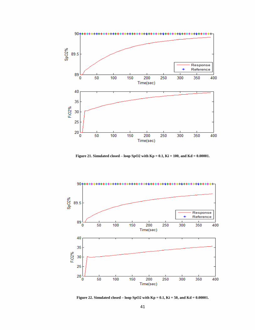
Figure 21. Simulated closed – loop SpO2 with Kp = 0.1, Ki = 100, and Kd = 0.00001.
Figure 22. Simulated closed – loop SpO2 with Kp = 0.1, Ki = 50, and Kd = 0.00001.
42
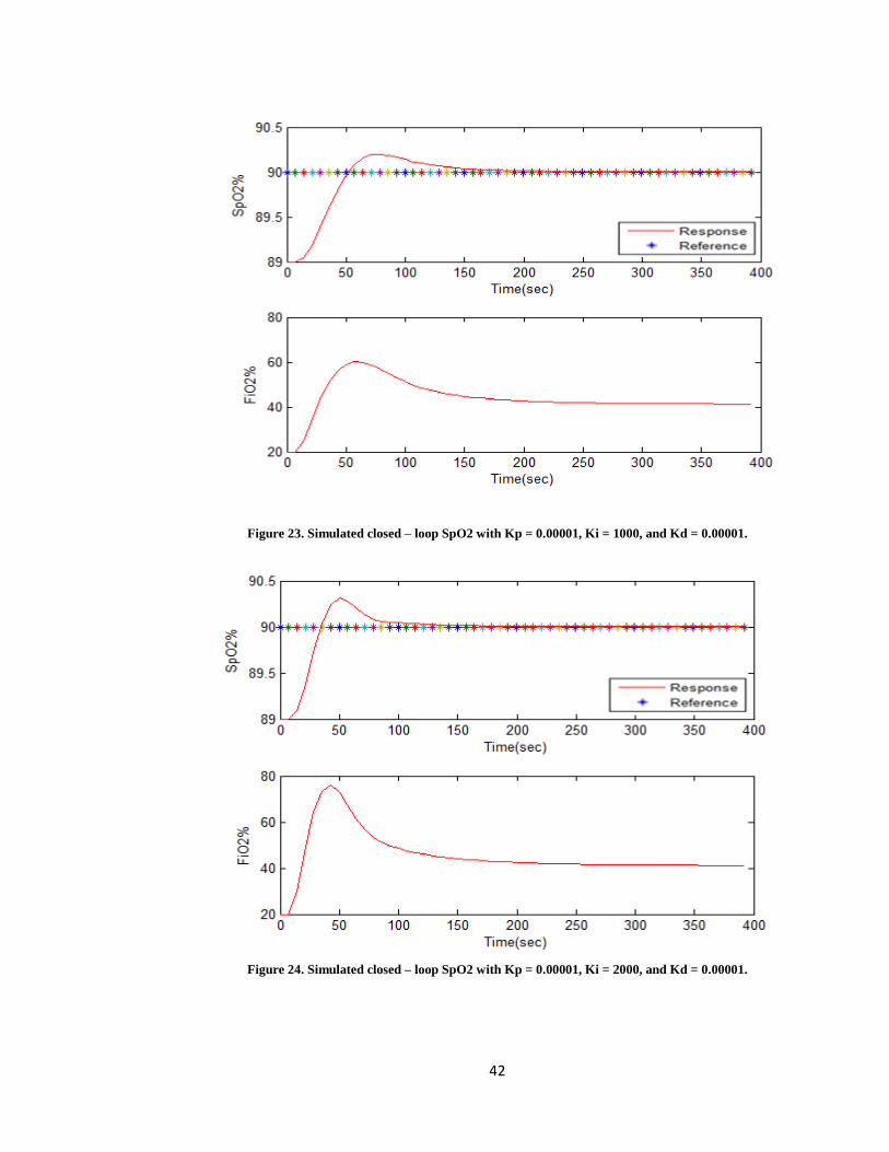
Figure 23. Simulated closed – loop SpO2 with Kp = 0.00001, Ki = 1000, and Kd = 0.00001.
Figure 24. Simulated closed – loop SpO2 with Kp = 0.00001, Ki = 2000, and Kd = 0.00001.
43
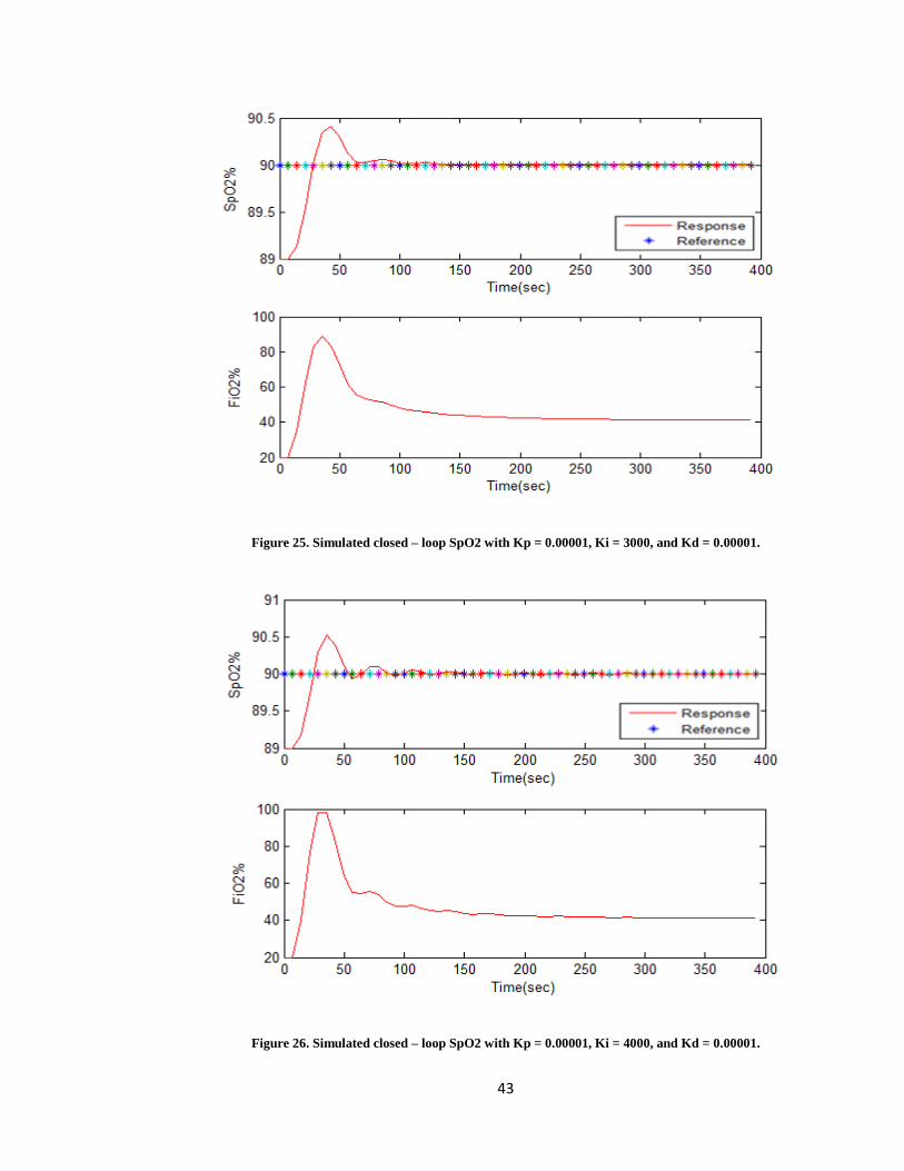
Figure 25. Simulated closed – loop SpO2 with Kp = 0.00001, Ki = 3000, and Kd = 0.00001.
Figure 26. Simulated closed – loop SpO2 with Kp = 0.00001, Ki = 4000, and Kd = 0.00001.

44
Figure 27. Simulated closed – loop SpO2 with Kp = 0.00001, Ki = 4500, and Kd = 0.00001.
Figure 28. Simulated closed – loop SpO2 with Kp = 0.00001, Ki = 5000, and Kd = 0.00001.

45
Figure 29. Simulated closed – loop SpO2 with Kp = 0.1, Ki = 1000, and Kd = 0.00001.
Figure 30. Simulated closed – loop SpO2 with Kp = 0.001, Ki = 1000, and Kd = 0. 001.

46
Figure 31. Simulated closed – loop SpO2 with Kp = 0. 1, Ki = 300, and Kd = 0.0001.
The control action in Eq (3.2) is simulated with tuning 𝐾𝑝,𝐾𝑖 and 𝐾𝑑 by
trial and error by matlab codes and applied as input 𝐹𝑖𝑂2 to the plant to get 𝑆𝑝𝑂2
with ranging from85 − 93 %. In this test, the best response is in Fig 16 because
there is no steady state error and minimum settling time and the value of 𝑆𝑝𝑂2
after 170 sec.
47
3.3. Model Predictive Control (MPC).
The main function of Model Predictive Control is to find the input signal that
best corresponds to some criteria which predict how the system will behave by
applying this signal. Model predictive control (MPC) was initially developed for
the control of large constrained systems with slow dynamics and has found
application in the process control industries. Model Predictive Control (MPC) is
an optimal control strategy based on numerical optimization. Future control inputs
and future plant responses are predicted using a system model and optimized at
regular intervals with respect to a performance index. Predictive control has
become the most widespread advanced control methodology current in use in this
industry. MPC has been developed so that stability, optimality, and robustness
properties are well understood. Advances in real – time computational abilities are
making this approach attractive for a wider range of applications. There are many
methods used to introduce a guarantee of stability into the design optimization.
The use of an infinite prediction horizon, Model Predictive Control (MPC), also
referred to as Receding Horizon Control and moving optimal control, has been
widely adapted in industry as an effective means to deal with multivariable
constrained control problems [31].
Most control design techniques need a control model of the plant with fixed
structure and parameters. If the control model were an exact, rather than an
approximate, description of the plant and there were no external disturbances, the

48
process could be controlled by an open – loop controller. Feedback is necessary in
process control because of the external perturbations and model inaccuracies in all
real processed.
The process of robust control is to design a controller which keeps the
stability and performance even the models inaccuracies. In order to model the
system, the most common techniques are frequency response uncertainty and
transfer function parametric uncertainty modeling. Figure 32 shows the block
diagram of the basic structure of MPC.
Figure 32. The Basic Structure of MPC.
49
3.3.1 MPC Strategy
The MPC Strategy is represented as in Figure 33.
1 – The future outputs for a determined horizon𝑁, called the prediction horizon,
are predicted at each instant 𝑡 using the process model. All the predicted outputs
rely on the known values which are past inputs and outputs and on the future
control signals (𝑡 + 𝑘), 𝑘 = 0,…… . , 𝑁 − 1 .
2 – The Optimizing used to calculate the future control signals in order to keep
the process as close as possible to the reference trajectory 𝑤(𝑡 + 𝑘) uses a
criterion that usually takes the form of a quadratic function of the error between
the predicted output signal and the predicted reference trajectory. An explicit
solution can be obtained if the criterion is quadratic, the model is linear and there
are no constraints. Otherwise an iterative optimization method has to be used.
3 – The control signal is sent to the process.
For this strategy, a model is used to predict the future plant outputs, based
on past and current values and on the proposed optimal future control actions.
These actions are calculated by the optimizer taking into account the cost function
(where the future tracking error is considered) as well as the constraints.
Transfer function models, are simple and is used in many control design
methods, and is valid for many kinds of processes. The state – space model is also
used in some formulations. The optimizer is another fundamental part of the
strategy as it provides control actions. If the cost is quadratic, its minimum can be

50
obtained as an explicit linear function of past inputs and outputs and the future
reference trajectory. In the presence of inequality constraints the solution has to
be obtained by more computationally taxing numerical algorithms.
In this work, we consider a mathematical system model of recovery from
desaturation events developed based on respiratory system. We use the step
response model of the respiratory system because it has one input, 𝐹𝑖𝑂2and one
output , 𝑆𝑝𝑂2 , that is developed and completed by Yu.
Figure 33. Receding Horizon strategy.
51
3.4 Dynamic Matrix Control
Dynamic Matrix Control (DMC) was the first model predictive control MPC
algorithm and available in almost all commercial industrial distributed control
systems. The DMC algorithm includes as one of its major components, a
technique to predict the future output of the system as a function of the inputs and
disturbances. This prediction capability is necessary to determine the optimal
future control inputs.
All the MPC algorithms possess common elements, and different options can be
chosen for each one of these elements giving rise to different algorithms. These
are three
- Prediction Model
- Objective Function
- Obtaining the control law
The model is the corner – stone of the MPC; a complete design should include the
necessary mechanisms for obtaining the best possible model, which should be
complete enough to fully capture the process dynamics. The use of the process
model is determined by the necessity to calculate the predicted output at future
instants ŷ (𝑡 + 𝑘).
The process model employed in this formulation is the step response of the plant
given as
52
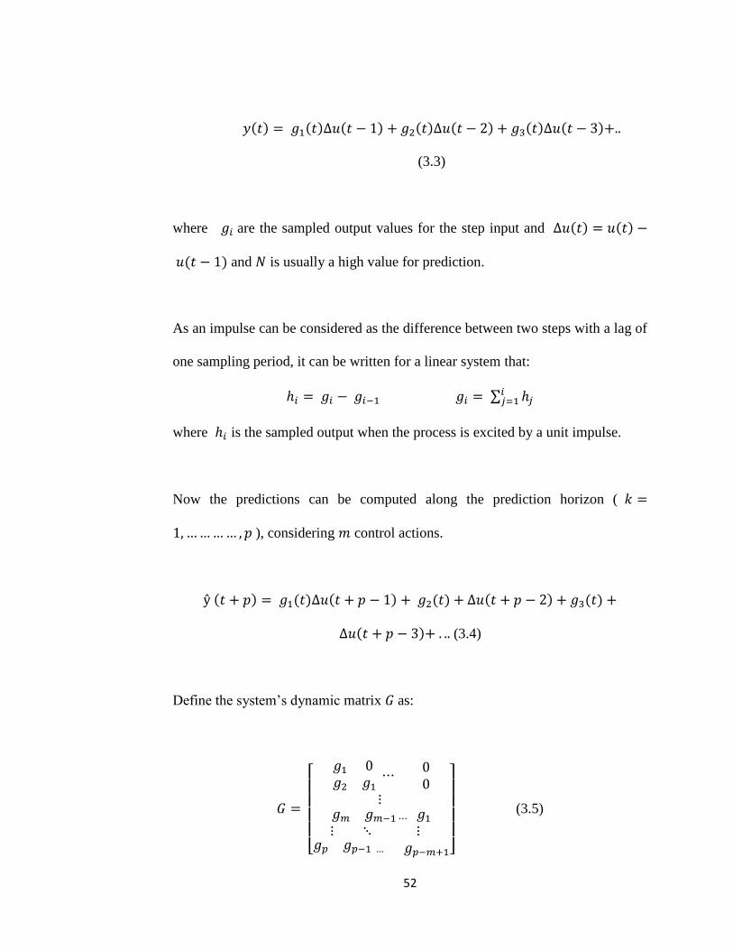
𝑦(𝑡) = 𝑔1(𝑡)∆𝑢(𝑡 − 1) + 𝑔2(𝑡)∆𝑢(𝑡 − 2) + 𝑔3(𝑡)∆𝑢(𝑡 − 3)+..
(3.3)
where 𝑔𝑖 are the sampled output values for the step input and ∆𝑢(𝑡) = 𝑢(𝑡) −
𝑢(𝑡 − 1) and 𝑁 is usually a high value for prediction.
As an impulse can be considered as the difference between two steps with a lag of
one sampling period, it can be written for a linear system that:
ℎ𝑖 = 𝑔𝑖 − 𝑔𝑖−1 𝑔𝑖 = ∑ ℎ𝑗𝑖𝑗=1
where ℎ𝑖 is the sampled output when the process is excited by a unit impulse.
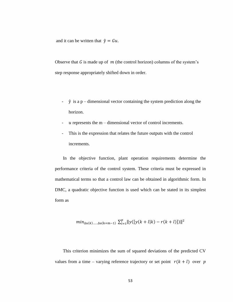
Now the predictions can be computed along the prediction horizon ( 𝑘 =
1, ………… , 𝑝 ), considering 𝑚 control actions.
ŷ (𝑡 + 𝑝) = 𝑔1(𝑡)∆𝑢(𝑡 + 𝑝 − 1) + 𝑔2(𝑡) + ∆𝑢(𝑡 + 𝑝 − 2) + 𝑔3(𝑡) +
∆𝑢(𝑡 + 𝑝 − 3)+ . .. (3.4)
Define the system’s dynamic matrix 𝐺 as:
𝐺 =
[
𝑔1 0𝑔2 𝑔1
⋯ 00
⋮ 𝑔𝑚 𝑔𝑚−1 ⋯ 𝑔1
⋮ ⋱ ⋮ 𝑔𝑝 𝑔𝑝−1 … 𝑔𝑝−𝑚+1]
(3.5)
53
and it can be written that ŷ = 𝐺𝑢.
Observe that 𝐺 is made up of 𝑚 (the control horizon) columns of the system’s
step response appropriately shifted down in order.
- ŷ is a p – dimensional vector containing the system prediction along the
horizon.
- 𝑢 represents the m – dimensional vector of control increments.
- This is the expression that relates the future outputs with the control
increments.
In the objective function, plant operation requirements determine the
performance criteria of the control system. These criteria must be expressed in
mathematical terms so that a control law can be obtained in algorithmic form. In
DMC, a quadratic objective function is used which can be stated in its simplest
form as
𝑚𝑖𝑛∆𝑢(𝑘)……∆u(k+m−1) ∑ ‖𝑦([𝑦(𝑘 + 𝑙|𝑘) − 𝑟(𝑘 + 𝑙)])‖2𝑝𝑙=1
This criterion minimizes the sum of squared deviations of the predicted CV
values from a time – varying reference trajectory or set point 𝑟(𝑘 + 𝑙) over 𝑝
54
future time steps. The quadratic criterion penalizes large deviations proportionally
more than smaller ones, so that on the average the output remains close to its
reference trajectory and large excursions are avoided.
where 𝑚 ≤ 𝑝 always. This means that DMC determines the next 𝑚 moves
only. The choices of 𝑚 and 𝑝 affect the closed – loop behavior. Moreover, 𝑚 ,
the number of degrees of freedom, has a dominant influence on the computational
effort.
Due to inherent process interactions, it is generally not possible to keep all
outputs close to their corresponding reference trajectories simultaneously.
Therefore, in practice only a subset of the outputs is controlled well at the expense
of larger excursion in others. This can be influenced transparently by including
weights in the objective function as follows:
𝑚𝑖𝑛∆𝑢(𝑘)……∆u(k+m−1) ∑ ‖𝛤𝑙𝑦([𝑦(𝑘 + 𝑙|𝑘) − 𝑟(𝑘 + 𝑙)])‖
2𝑝𝑙=1 (3.6)
If a system with two outputs 𝑦1 and 𝑦2 , and constant diagonal weight
matrices of the form
𝛤𝑙𝑦
= [𝑙1 00 𝑙2
]
55
The objective becomes
𝑚𝑖𝑛∆𝑢(𝑘)……∆u(k+m−1) {𝑙12 ∑ [( [𝑦1(𝑘 + 𝑙|𝑘) − 𝑟1(𝑘 + 𝑙)])]2𝑝
𝑙=1 +
{𝑙22 ∑ [( [𝑦2(𝑘 + 𝑙|𝑘) − 𝑟2(𝑘 + 𝑙)])]2𝑝
𝑙=1 (3.7)
Thus, the larger the weight is for a particular output, the larger is the contribution
of its sum of squared deviations to the objective. This will make the controller
bring the corresponding output closer to its reference trajectory.
Finally, the manipulated variable moves that make the output follow a given
trajectory could be too severe to be acceptable in practice. This can be corrected
by adding a penalty term for the manipulated variable moves to the objectives as
the following:
𝑚𝑖𝑛∆𝑢(𝑘) ∑ ‖ 𝛤𝑙𝑦[( [𝑦(𝑘 + 𝑙|𝑘) − 𝑟(𝑘 + 𝑙)])]‖
2𝑝𝑙=1 + ∑ ‖ 𝛤𝑙
𝑢[∆𝑢(𝑘 + 𝑙 − 1]‖2𝑚𝑙=1
(3.8)
Note that the larger the elements of the matrix 𝛤𝑙𝑢 are the smallest the resulting
moves will be, and consequently, the output trajectories will not be followed as
closely. Thus, the relative magnitude of 𝛤𝑙𝑦
and 𝛤𝑙𝑢 will determine the trade –
off between following the trajectory closely and reducing the action of the
manipulated variables.
56
For any assumed set of present and future control moves ∆𝑢(𝑡), ∆𝑢(𝑡 +
1),…… . , ∆𝑢(𝑡 + 𝑚 − 1) then the future behavior of the process outputs 𝑦(𝑡 +
1), 𝑦, … . , 𝑦(𝑘 + 𝑝|𝑘) can be predicted over a horizon 𝑃 . The 𝑚 present and
future control moves (𝑚 ≤ 𝑝) are computed to minimize a quadratic objective of
the form as in Eq (3.6).
where 𝛤𝑙𝑦
and 𝛤𝑙𝑢 are weighting matrices to penalize particular components of
𝑦 or 𝑢 at certain future time intervals. 𝑟(𝑘 + 1) is the vector of future reference
values (set point). At the first sampling, the 𝑚 control moves and ∆𝑢(𝑘) is
implemented. At the next sampling interval, new values of the measured output
are obtained, the control horizon is shifted forward by one step, and the same
computations are repeated. The moving horizon is leading to get the control law,
the feedback control law is
∆𝑢(𝑘) = 𝐾𝑀𝑃𝐶𝐸𝑝(𝑘 + 1|𝑘) (3.12)
where 𝐸𝑝(𝑘 + 1|𝑘) is the vector of predicted future errors over the horizon 𝑃
which would result if all present and future manipulated variable moves were
equal to zero ∆𝑢(𝑘) = ∆𝑢(𝑘 + 1) = ⋯ = 0.
The nominal stability of the closed – loop system in the open – loop stable plants
depends only on 𝐾𝑀𝑃𝐶 which depends on the values of horizon 𝑝 and, the number
of 𝑚 and the weighting matrices 𝛤𝑙𝑦
and 𝛤𝑙𝑢. The value of 𝛤𝑙
𝑢 is used as a tuning
parameter which means that increasing 𝛤𝑙𝑢 always has the effect of making the
control action less aggressive.
57
The objective of a DMC controller is to drive the output as close to the set
point as possible in a least –squares sense with the possibility of the inclusion of a
penalty term on the input moves. Disturbances and modeling errors may lead to
deviations between the predicted behavior and actual observed behavior so that
the computed manipulated variable moves are actually implemented. The DMC
algorithm includes as one of its major components a technique to predict the
future output of the system as a function of the inputs and disturbances. The
prediction is necessary to determine the optimal future control input.
The optimization problem with a quadratic objective and linear inequalities,
which it has defined is a Quadratic Program. By converting to the standard QP
formulation the DMC problem becomes:
𝑚𝑖𝑛∆𝑢(𝑘) ∆𝑢(𝑘)𝑇 𝐻𝑢∆𝑢(𝑘) − 𝑔(𝑘 + 1)𝑇 ∆𝑢(𝑘) (3.13)
where the Hessian of the QP is
𝐻𝑢 = 𝐷𝑇𝛤𝑙𝑦𝑇
𝛤𝑙𝑦𝐷 + 𝛤𝑙
𝑢𝑇 𝛤𝑙
𝑢 (3.14)
and the gradient vector is
g(k + 1) = 2 𝐷𝑇 𝛤𝑙𝑦𝑇
𝛤𝑙𝑦 𝐸𝑝(𝑘 + 1) (3.15)
58
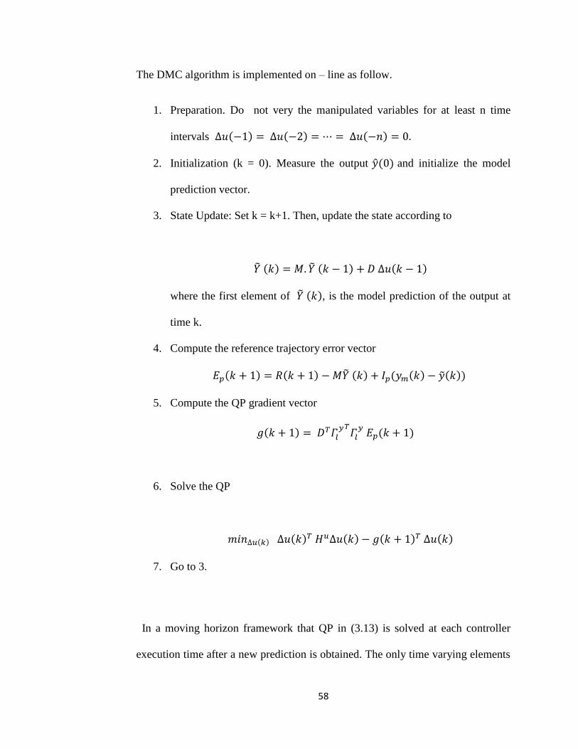
The DMC algorithm is implemented on – line as follow.
1. Preparation. Do not very the manipulated variables for at least n time
intervals ∆𝑢(−1) = ∆𝑢(−2) = ⋯ = ∆𝑢(−𝑛) = 0.
2. Initialization (k = 0). Measure the output �̂�(0) and initialize the model
prediction vector.
3. State Update: Set k = k+1. Then, update the state according to
�̃� (𝑘) = 𝑀. �̃� (𝑘 − 1) + 𝐷 ∆𝑢(𝑘 − 1)
where the first element of �̃� (𝑘), is the model prediction of the output at
time k.
4. Compute the reference trajectory error vector
𝐸𝑝(𝑘 + 1) = 𝑅(𝑘 + 1) − 𝑀�̃� (𝑘) + 𝐼𝑝(𝑦𝑚(𝑘) − �̃�(𝑘))
5. Compute the QP gradient vector
𝑔(𝑘 + 1) = 𝐷𝑇𝛤𝑙𝑦𝑇
𝛤𝑙𝑦 𝐸𝑝(𝑘 + 1)
6. Solve the QP
𝑚𝑖𝑛∆𝑢(𝑘) ∆𝑢(𝑘)𝑇 𝐻𝑢∆𝑢(𝑘) − 𝑔(𝑘 + 1)𝑇 ∆𝑢(𝑘)
7. Go to 3.
In a moving horizon framework that QP in (3.13) is solved at each controller
execution time after a new prediction is obtained. The only time varying elements
59
in this problem are the vectors 𝐸𝑝(𝑘 + 1) (or equivalently g (k+1)). That is, the
Hessian 𝐻 of the QP remains constant for all executions. In that case, a parametric
QP algorithm which employs the pre-inverted Hessian in its computations is
preferable in order to reduce on-line computation effort. Of course, in case either
𝛤𝑙𝑦
or 𝛤𝑙𝑢 (or the step response coefficients) need to be updated, or the model’s
step response coefficients have changed, the Hessian must be recomputed and
inverted in background mode in order not to increase the on – line computational
requirements.
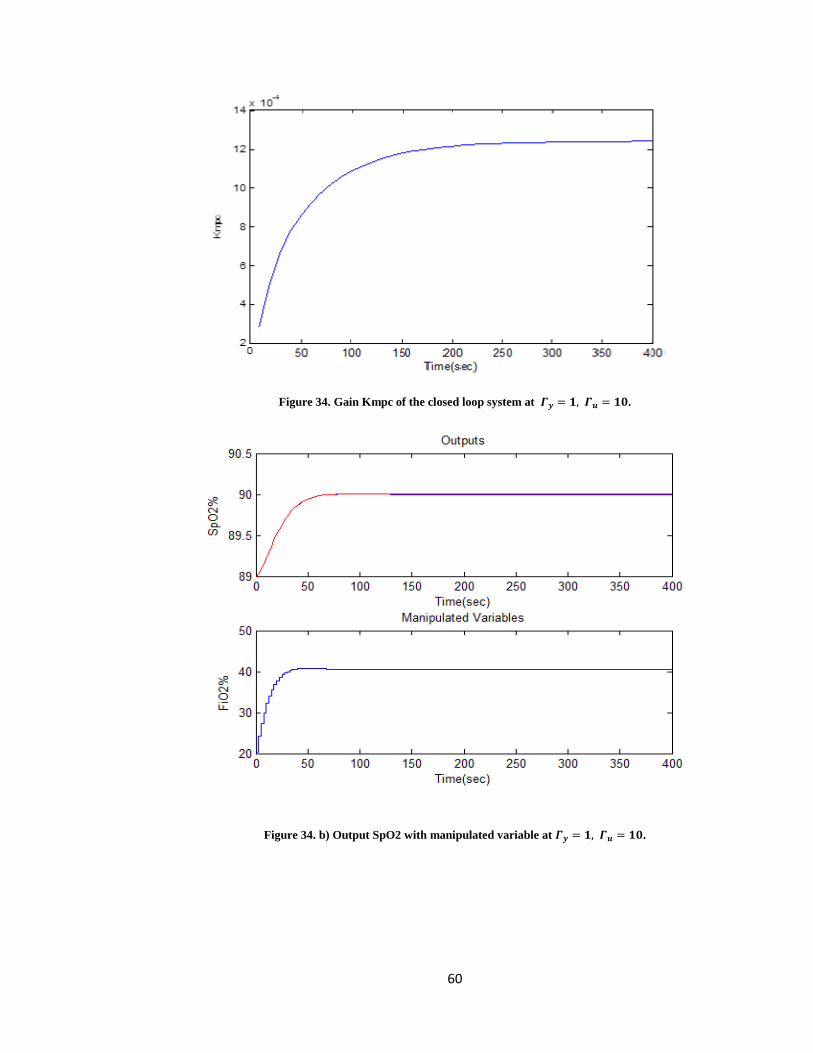
60
Figure 34. Gain Kmpc of the closed loop system at 𝜞𝒚 = 𝟏, 𝜞𝒖 = 𝟏𝟎.
Figure 34. b) Output SpO2 with manipulated variable at 𝜞𝒚 = 𝟏, 𝜞𝒖 = 𝟏𝟎.
61
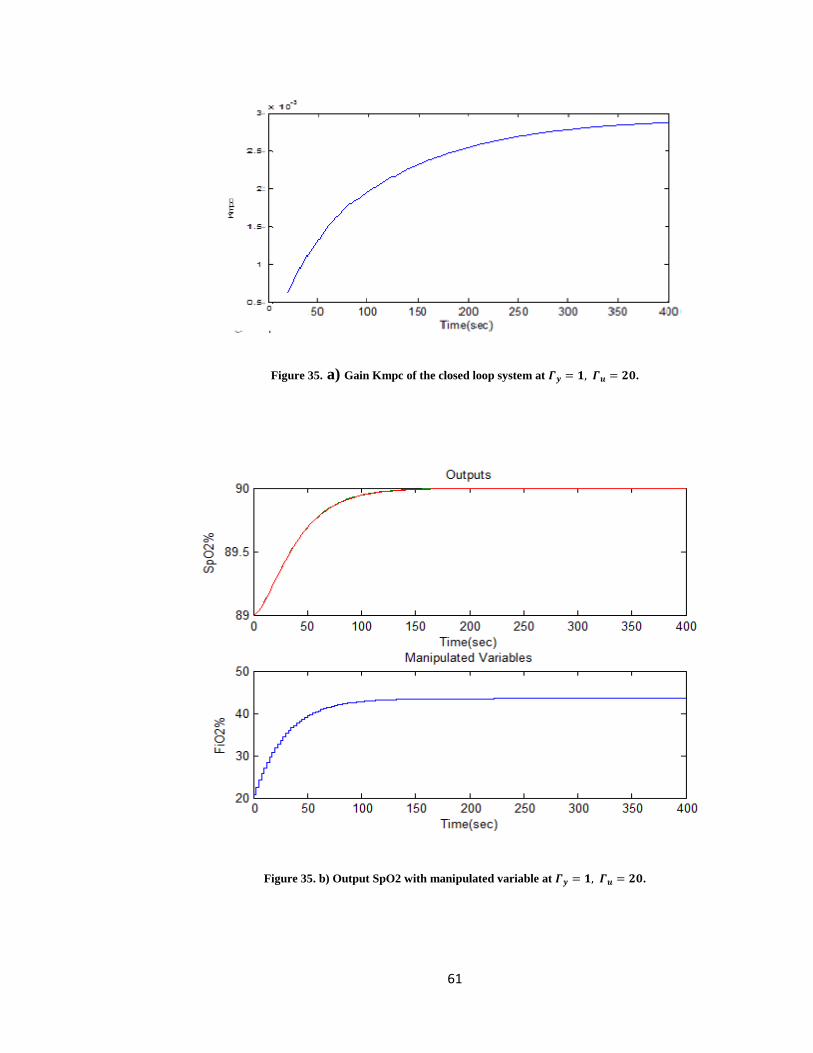
Figure 35. a) Gain Kmpc of the closed loop system at 𝜞𝒚 = 𝟏, 𝜞𝒖 = 𝟐𝟎.
Figure 35. b) Output SpO2 with manipulated variable at 𝜞𝒚 = 𝟏, 𝜞𝒖 = 𝟐𝟎.
62
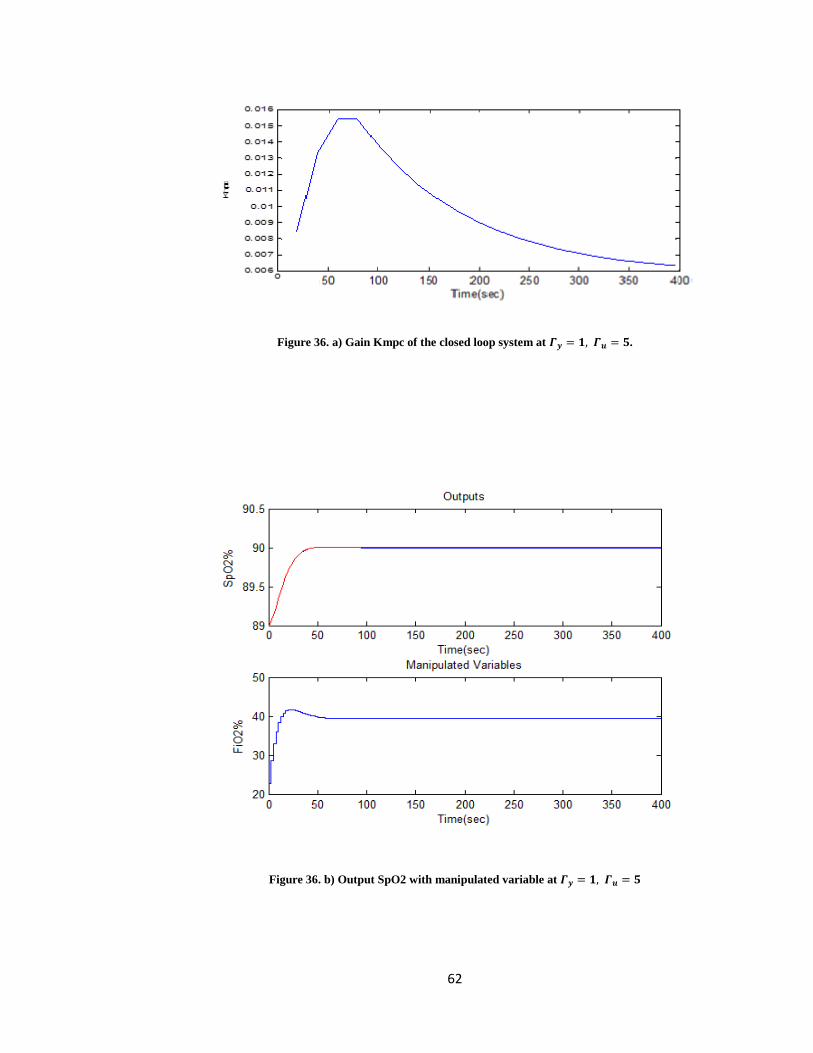
Figure 36. a) Gain Kmpc of the closed loop system at 𝜞𝒚 = 𝟏, 𝜞𝒖 = 𝟓.
Figure 36. b) Output SpO2 with manipulated variable at 𝜞𝒚 = 𝟏, 𝜞𝒖 = 𝟓
63
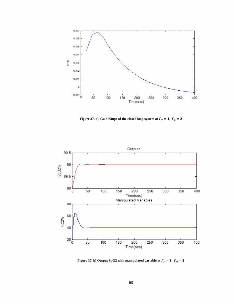
Figure 37. a) Gain Kmpc of the closed loop system at 𝜞𝒚 = 𝟏, 𝜞𝒖 = 𝟐
Figure 37. b) Output SpO2 with manipulated variable at 𝜞𝒚 = 𝟏, 𝜞𝒖 = 𝟐

64
Not that the larger the elements of the matrix 𝛤𝑙𝑢 were, the smaller the resulting
moves will be, and consequently, the output trajectories didn’t follow as closely.
Therefore, the relative magnitude of 𝛤𝑙𝑦
and 𝛤𝑙𝑢 determined the trade – off
between the trajectory closely and reduced the action of the manipulated variable.
The best response is in Fig (34) because there is no steady state error and
minimum settling time and the value of 𝑆𝑝𝑂2 after 65 sec.
65
Chapter 4: Robustness
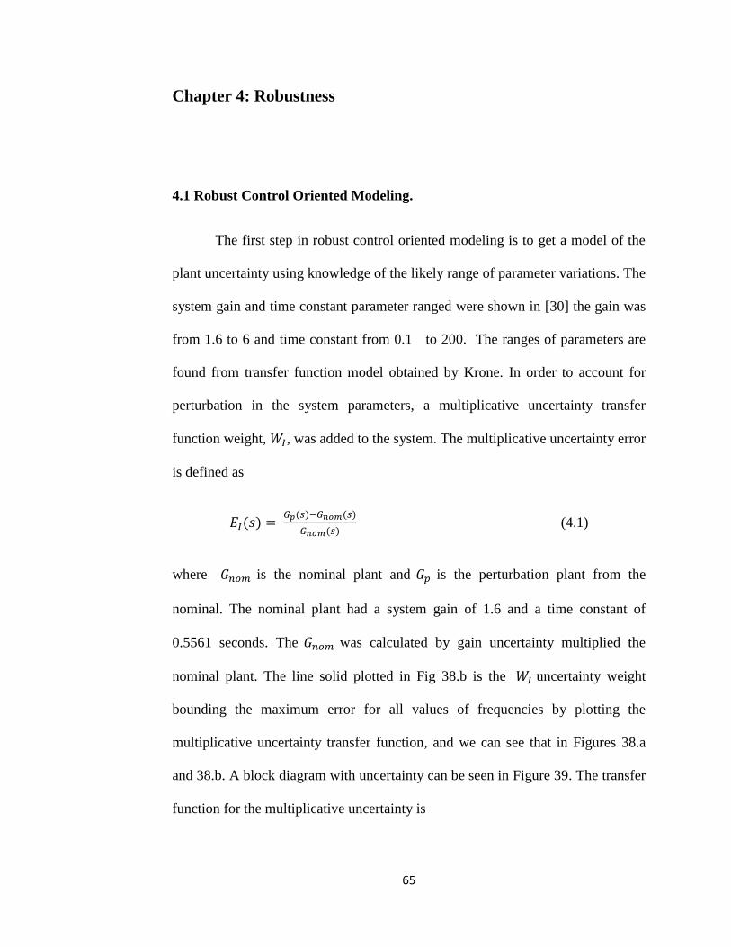
4.1 Robust Control Oriented Modeling.
The first step in robust control oriented modeling is to get a model of the
plant uncertainty using knowledge of the likely range of parameter variations. The
system gain and time constant parameter ranged were shown in [30] the gain was
from 1.6 to 6 and time constant from 0.1 to 200. The ranges of parameters are
found from transfer function model obtained by Krone. In order to account for
perturbation in the system parameters, a multiplicative uncertainty transfer
function weight, 𝑊𝐼, was added to the system. The multiplicative uncertainty error
is defined as
𝐸𝐼(𝑠) = 𝐺𝑝(𝑠)−𝐺𝑛𝑜𝑚(𝑠)
𝐺𝑛𝑜𝑚(𝑠) (4.1)
where 𝐺𝑛𝑜𝑚 is the nominal plant and 𝐺𝑝 is the perturbation plant from the
nominal. The nominal plant had a system gain of 1.6 and a time constant of
0.5561 seconds. The 𝐺𝑛𝑜𝑚 was calculated by gain uncertainty multiplied the
nominal plant. The line solid plotted in Fig 38.b is the 𝑊𝐼 uncertainty weight
bounding the maximum error for all values of frequencies by plotting the
multiplicative uncertainty transfer function, and we can see that in Figures 38.a
and 38.b. A block diagram with uncertainty can be seen in Figure 39. The transfer
function for the multiplicative uncertainty is
66
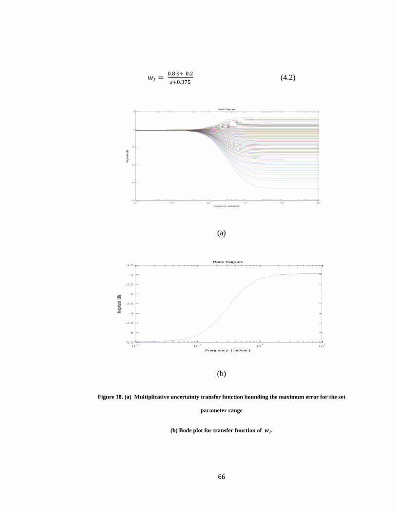
𝑤𝐼 = 0.8 𝑠+ 0.2
𝑠+0.375 (4.2)
(a)
(b)
Figure 38. (a) Multiplicative uncertainty transfer function bounding the maximum error for the set
parameter range
(b) Bode plot for transfer function of 𝒘𝑰.
10-2
10-1
100
101
102
103
-25
-20
-15
-10
-5
0
Mag
nitu
de (d
B)
Bode Diagram
Frequency (rad/sec)
10-2
10-1
100
101
-5.5
-5
-4.5
-4
-3.5
-3
-2.5
-2
-1.5
Magn
itude
(dB)
Bode Diagram
Frequency (rad/sec)
67
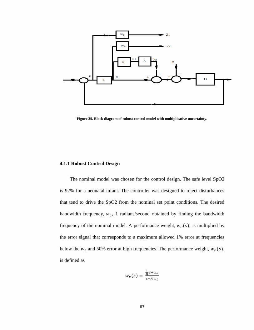
Figure 39. Block diagram of robust control model with multiplicative uncertainty.
4.1.1 Robust Control Design
The nominal model was chosen for the control design. The safe level SpO2
is 92% for a neonatal infant. The controller was designed to reject disturbances
that tend to drive the SpO2 from the nominal set point conditions. The desired
bandwidth frequency, 𝜔𝑏 , 1 radians/second obtained by finding the bandwidth
frequency of the nominal model. A performance weight, 𝑤𝑃(𝑠), is multiplied by
the error signal that corresponds to a maximum allowed 1% error at frequencies
below the 𝑤𝑏 and 50% error at high frequencies. The performance weight, 𝑤𝑃(𝑠),
is defined as
𝑤𝑃(𝑠) = 1
𝑀 𝑠+𝜔𝑏
𝑠+𝐴 𝜔𝑏
68
where 𝑀 is high frequency , 𝐴 is the low frequency error , and 𝜔𝑏 is band width
for |1
𝑤𝑝(𝑗𝑤)|. The |𝑆(𝑗𝑤)| is the magnitude of error the system and |
1
𝑤𝑝(𝑗𝑤)| be
upper bound on S or largest acceptable error is
|𝑆(𝑗𝑤)| < |1
𝑤𝑝(𝑗𝑤)| ∀ 𝜔
and for condition above we can get parameters of 𝑤𝑃(𝑠) as
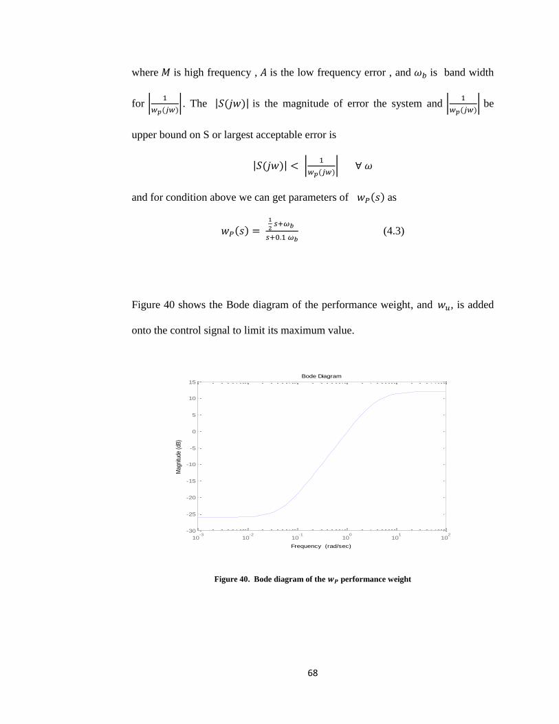
𝑤𝑃(𝑠) = 1
2 𝑠+𝜔𝑏
𝑠+0.1 𝜔𝑏 (4.3)
Figure 40 shows the Bode diagram of the performance weight, and 𝑤𝑢, is added
onto the control signal to limit its maximum value.
Figure 40. Bode diagram of the 𝒘𝑷 performance weight
10-3
10-2
10-1
100
101
102
-30
-25
-20
-15
-10
-5
0
5
10
15
Mag
nitu
de (
dB)
Bode Diagram
Frequency (rad/sec)
69
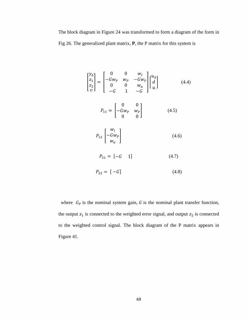
The block diagram in Figure 24 was transformed to form a diagram of the form in
Fig 26. The generalized plant matrix, P, the P matrix for this system is
[
𝑦∆
𝑧1
𝑧2𝑣
] = [
0 0 𝑤𝐼
−𝐺𝑤𝑃 𝑤𝑃 −𝐺𝑤𝑃
0 0 𝑤𝑢
−𝐺 1 −𝐺
] [𝑢∆
𝑑𝑢
] (4.4)
𝑃11 = [0 0
−𝐺𝑤𝑃 𝑤𝑃
0 0] (4.5)
𝑃12 [
𝑤𝐼
−𝐺𝑤𝑃
𝑤𝑢
] (4.6)
𝑃21 = [−𝐺 1] (4.7)
𝑃22 = [ −𝐺] (4.8)
where 𝐺𝑃 is the nominal system gain, 𝐺 is the nominal plant transfer function,
the output 𝑧1 is connected to the weighted error signal, and output 𝑧2 is connected
to the weighted control signal. The block diagram of the P matrix appears in
Figure 41.
70
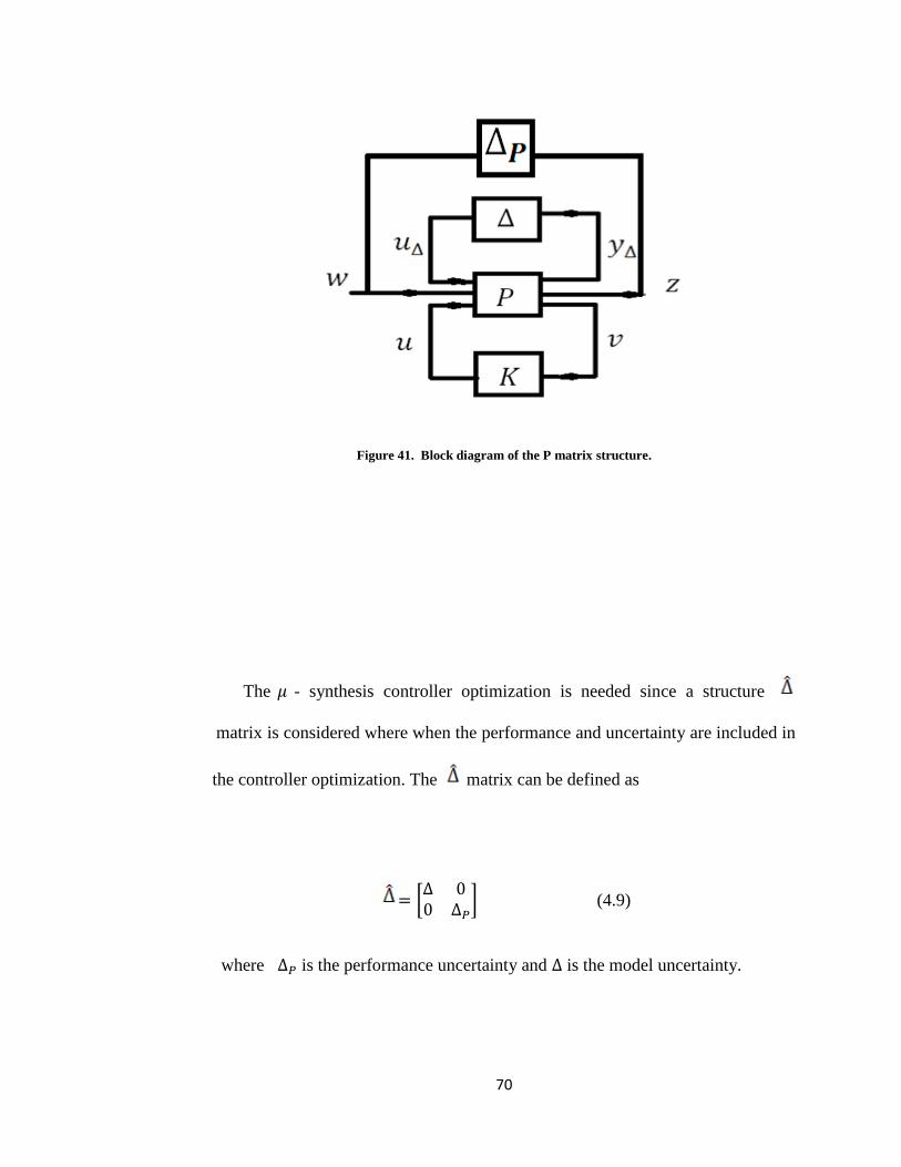
Figure 41. Block diagram of the P matrix structure.
The 𝜇 - synthesis controller optimization is needed since a structure
matrix is considered where when the performance and uncertainty are included in
the controller optimization. The matrix can be defined as
= [∆ 00 ∆𝑃
] (4.9)
where ∆𝑃 is the performance uncertainty and ∆ is the model uncertainty.
71
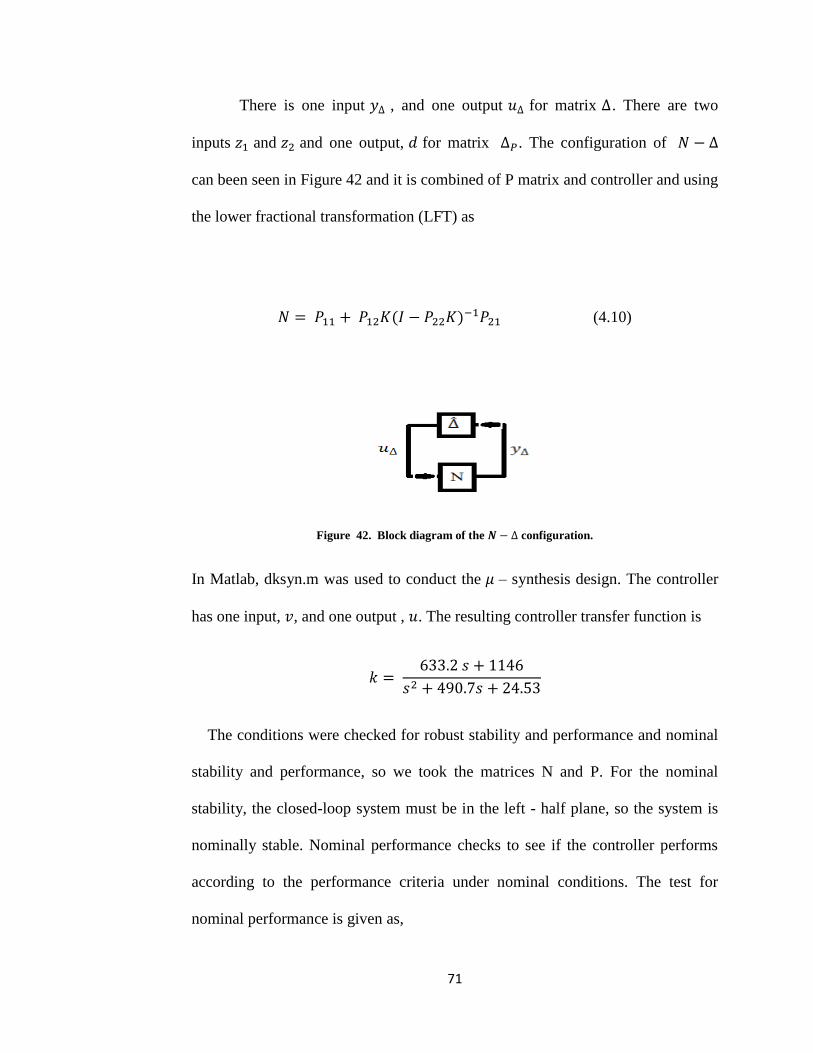
There is one input 𝑦∆ , and one output 𝑢∆ for matrix ∆. There are two
inputs 𝑧1 and 𝑧2 and one output, 𝑑 for matrix ∆𝑃. The configuration of 𝑁 − ∆
can been seen in Figure 42 and it is combined of P matrix and controller and using
the lower fractional transformation (LFT) as
𝑁 = 𝑃11 + 𝑃12𝐾(𝐼 − 𝑃22𝐾)−1𝑃21 (4.10)
Figure 42. Block diagram of the 𝑵 − ∆ configuration.
In Matlab, dksyn.m was used to conduct the 𝜇 – synthesis design. The controller
has one input, 𝑣, and one output , 𝑢. The resulting controller transfer function is
𝑘 = 633.2 𝑠 + 1146
𝑠2 + 490.7𝑠 + 24.53
The conditions were checked for robust stability and performance and nominal
stability and performance, so we took the matrices N and P. For the nominal
stability, the closed-loop system must be in the left - half plane, so the system is
nominally stable. Nominal performance checks to see if the controller performs
according to the performance criteria under nominal conditions. The test for
nominal performance is given as,

72
𝑁𝑃 = |𝑊𝑃(𝑗𝑤)(1 + 𝐾𝐺)−1|∞
To check the nominal performance, the inequality must hold for frequencies [32].
‖𝑁22‖∞ ≤ 1 (4.11)
The system is nominally stable if only if the values of 𝑁22 less than one and
can be seen the nominal performance by plotting the H-infinty norm as shown in
Figure 43.
Figure 43. The H-infinity norm of 𝑵𝟐𝟐 is less than one for all frequencies.
10-8
10-6
10-4
10-2
100
102
104
-140
-120
-100
-80
-60
-40
-20
0
NP
Frequency (rad/sec)
Sin
gula
r V
alue
s (d
B)
73
For the robust stability , 𝑁11 is less or equal one for all frequencies and that the
system is robust stable [31]. The equation for robust stability is
𝑅𝑆 = |𝑊𝑖(𝑗𝑤)𝐾𝐺(1 + 𝐾𝐺)−1|∞
The inequality
‖𝑁11‖∞ ≤ 1 (4.12 )
To achieve robust stability the maximum value from Eq (4.12) must be less than
one.
The h-infinity norm of 𝑁11 can bee seen in Figure (44 ).
Robust performance checks to see if the controller performs according to the
performance criteria over a range of input. Robust performance can be checked
using Eq (4.13).
𝑅𝑃 = |𝑊𝑃(𝑗𝑤)(1 + 𝐾𝐺)−1|∞
+ |𝑊𝑖(𝑗𝑤)𝐾𝐺(1 + 𝐾𝐺)−1|∞
(4.13)
𝜇 (𝑁, ) < 1 (4.14)
The recursive algorithms and the iterative algorithms can estimate the parameters
of linear regressive models from observation data [34-36].

74
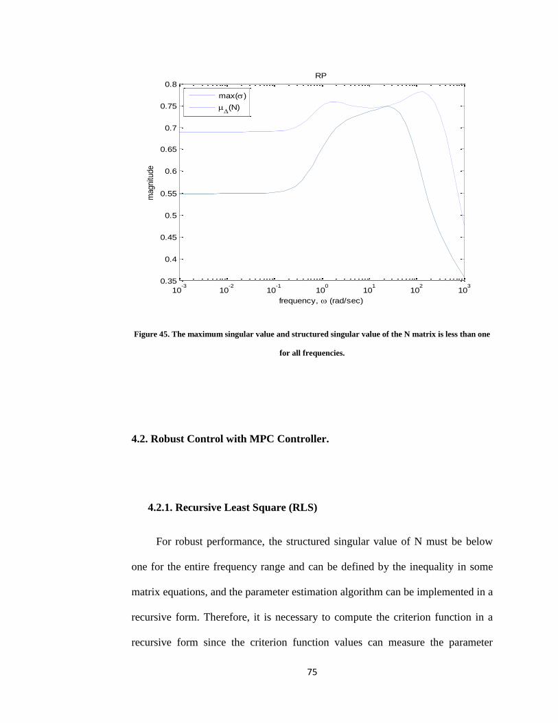
The 𝜇-synthesis controller is found to have robust performance which
can bee seen in Figure (45). We can see that the amplitudes of max singular value
and 𝜇-synthesis are less than one and that means that the robust controller is
found to be able to achieve a desirable performance given the level of uncetainty
in the system that was modeled.
Figure 44. The H-infinity norm of 𝑵𝟏𝟏 is less than one for all frequencies for the 𝝁-synthesis controller.
10-1
100
101
102
103
104
-40
-35
-30
-25
-20
-15
-10
-5
0
RS
Frequency (rad/sec)
Sin
gula
r V
alu
es (
dB
)
75
Figure 45. The maximum singular value and structured singular value of the N matrix is less than one
for all frequencies.
4.2. Robust Control with MPC Controller.
4.2.1. Recursive Least Square (RLS)
For robust performance, the structured singular value of N must be below
one for the entire frequency range and can be defined by the inequality in some
matrix equations, and the parameter estimation algorithm can be implemented in a
recursive form. Therefore, it is necessary to compute the criterion function in a
recursive form since the criterion function values can measure the parameter
10-3
10-2
10-1
100
101
102
103
0.35
0.4
0.45
0.5
0.55
0.6
0.65
0.7
0.75
0.8
frequency, (rad/sec)
magnitu
de
RP
max()
(N)
76
estimation accuracy [37]. To estimate the model control system that in model
predictive section, we must find the coefficients of the polynomial of estimate
system. This is usually accomplished by assuming a discrete time form for the
control system model and then using a recursive estimation algorithm to obtain
estimates of the parameters of the model. To determine the coefficient of the
model parameters using the recursive least square, a scheme of new input/output
data becomes available at each sample interval. The model based on past
information (summarized in 𝜃 ,(𝑡 − 1) as a vector of unknown) is used to obtain
an estimate 𝑦(𝑡) to generate an error 𝜀(𝑡). This in turn generates an update to the
model which corrects 𝜃 ,(𝑡 − 1) to the new value𝜃 ,(𝑡). This recursive “predictor –
corrector” form allows significant saving in computation, requiring the storage of
all previous data. It is both efficient and elegant to merely store the “old” estimate
calculated at time𝑡, denoted b 𝜃 ,(𝑡), and to obtain the “new” estimates 𝜃 ,(𝑡 + 1)
by an updating step involving the new observation only. Recursive Least Square
(RLS) is used as on – line identification [38 - 39].
The algorithm below was used to calculate the recursive least square.
(i) From 𝑥(𝑡 + 1) using the new data.
(ii) From 𝜀(𝑡 + 1) using 𝑋𝑇(𝑡 + 1).
𝜀(𝑡 + 1) = 𝑦(𝑡 + 1) − 𝑋𝑇(𝑡 + 1) 𝜃 ,(𝑡)
77
(iii) From using
𝑝(𝑡 + 1) = 𝑝(𝑡) [𝐼𝑚 + 𝑥(𝑡 + 1)𝑋𝑇(𝑡 + 1)𝑝(𝑡 + 1)
1 + 𝑋𝑇(𝑡 + 1)𝑝(𝑡)𝑥(𝑡 + 1)]
(iv) Update 𝜃 ,(𝑡)
𝜃 ,(𝑡 + 1) = 𝜃 ,(𝑡) + 𝑝(𝑡 + 1)𝑥(𝑡 + 1) 𝜀(𝑡 + 1)
(v) Wait for the next time step to elapse and loop back to step (i).
Now, we used RLS in the algorithm above to get an estimate of the control
modeling system to get the discrete differential equation 𝑦(𝑛) and after that to
convert the discrete equation to z-domain and after that convert to s- domain by
using bilinear equation as shown in Figure 46.
The discrete differential equation for control in MPC after RLS algorithm is
𝑢(𝑛) = 0.01529 𝑢(𝑛 − 1) + 0.0075 𝑢(𝑛 − 2) + 0.7226 𝑢(𝑛 − 3)
+ 0.5515 𝑒(𝑛 − 1) + 0.5515 𝑒(𝑛 − 2)
The Laplace transforms function for control in MPC after converting z- transform
to s – domain is
𝑢(𝑠)
𝑒(𝑠)=
0.1234 𝑠2 + 0.8769 𝑠 + 1.879
𝑠3 + 0.3257 𝑠2 + 4.3313 𝑠 + 0.08534
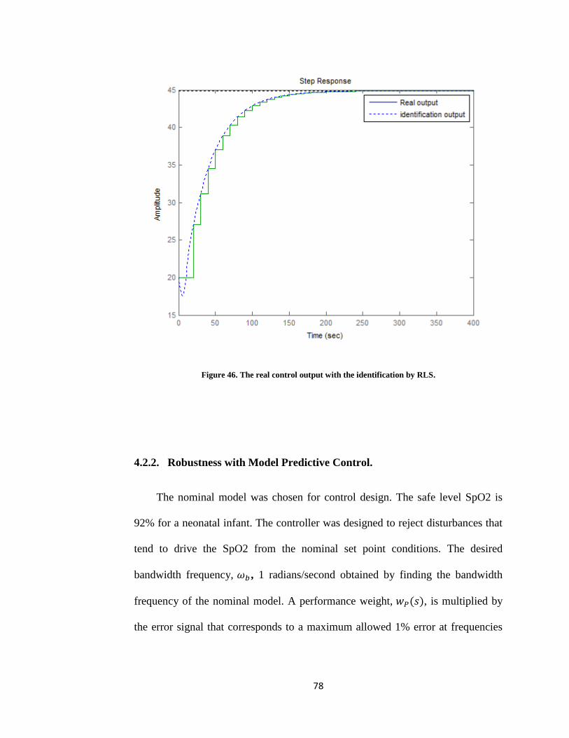
78
Figure 46. The real control output with the identification by RLS.
4.2.2. Robustness with Model Predictive Control.
The nominal model was chosen for control design. The safe level SpO2 is
92% for a neonatal infant. The controller was designed to reject disturbances that
tend to drive the SpO2 from the nominal set point conditions. The desired
bandwidth frequency, 𝜔𝑏 , 1 radians/second obtained by finding the bandwidth
frequency of the nominal model. A performance weight, 𝑤𝑃(𝑠), is multiplied by
the error signal that corresponds to a maximum allowed 1% error at frequencies

79
below the 𝑤𝑏 and 50% error at high frequencies. The performance weight, 𝑤𝑃(𝑠),
is defined as
𝑤𝑃(𝑠) = 1
𝑀 𝑠+𝜔𝑏
𝑠+𝐴 𝜔𝑏
where 𝑀 is high frequency , 𝐴 is the low frequency error , and 𝜔𝑏 is band width
for |1
𝑤𝑝(𝑗𝑤)|. The |𝑆(𝑗𝑤)| is the magnitude of error the system and |
1
𝑤𝑝(𝑗𝑤)| be
upper bound on S or largest acceptable error is
|𝑆(𝑗𝑤)| < |1
𝑤𝑝(𝑗𝑤)| ∀ 𝜔
and for condition above we can get parameters of 𝑤𝑃(𝑠) as
𝑤𝑃(𝑠) = 1
6 𝑠+0.05
𝑠+0.5∗0.05 (4.3)
Figure 47 shows the Bode diagram of the performance weight and 𝑤𝑢, is added
onto the control signal to limit its maximum value.

80
Figure 47. Bode diagram of the 𝒘𝑷 performance weight.
The conditions were checked for robust stability and performance and nominal
stability and performance, so we took the matrices N and P. For the nominal
stability, the closed-loop system must be in the left - half plane, so the system is
nominally stable. We performed nominal performance checks to see if the
controller performs according to the performance criteria under nominal
conditions. The test for nominal performance is given as
𝑁𝑃 = |𝑊𝑃(𝑗𝑤)(1 + 𝐾𝐺)−1|∞
To check the nominal performance, the inequality must hold for frequencies [32].
10-3
10-2
10-1
100
101
-10
-5
0
5
10
15
20
Magnitu
de (
dB
)
Bode Diagram
Frequency (rad/sec)
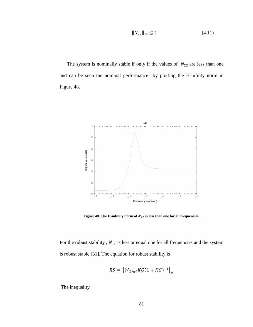
81
‖𝑁22‖∞ ≤ 1 (4.11)
The system is nominally stable if only if the values of 𝑁22 are less than one
and can be seen the nominal performance by plotting the H-infinty norm in
Figure 48.
Figure 48. The H-infinity norm of 𝑵𝟐𝟐 is less than one for all frequencies.
For the robust stability , 𝑁11 is less or equal one for all frequencies and the system
is robust stable [31]. The equation for robust stability is
𝑅𝑆 = |𝑊𝑖(𝑗𝑤)𝐾𝐺(1 + 𝐾𝐺)−1|∞
The inequality
10-3
10-2
10-1
100
101
102
103
-20
-18
-16
-14
-12
-10
-8
NP
Frequency (rad/sec)
Sin
gula
r V
alu
es (
dB
)

82
‖𝑁11‖∞ ≤ 1 (4.12 )
To achieve robust stability the maximum value from Eq (4.12) must be less than
one.
The h-infinity norm of 𝑁11 can bee seen in Figure (49 ).
Robust performance checks to see if the controller performs according to the
performance criteria over a range of input. Robust performance can be checked
using Eq (4.13).
𝑅𝑃 = |𝑊𝑃(𝑗𝑤)(1 + 𝐾𝐺)−1|∞
+ |𝑊𝑖(𝑗𝑤)𝐾𝐺(1 + 𝐾𝐺)−1|∞
(4.13)
For robust performance, the structured singular value of N must be below
one for the entire frequency range and can be defined by the inequality
𝜇 (𝑁, ) < 1 (4.14)
The 𝜇-synthesis controller is found to have robust performance which
can bee seen in Figure 50. We can see that the amplitudes of max singular value
and 𝜇-synthesis are less than one and that means that the robust controller is
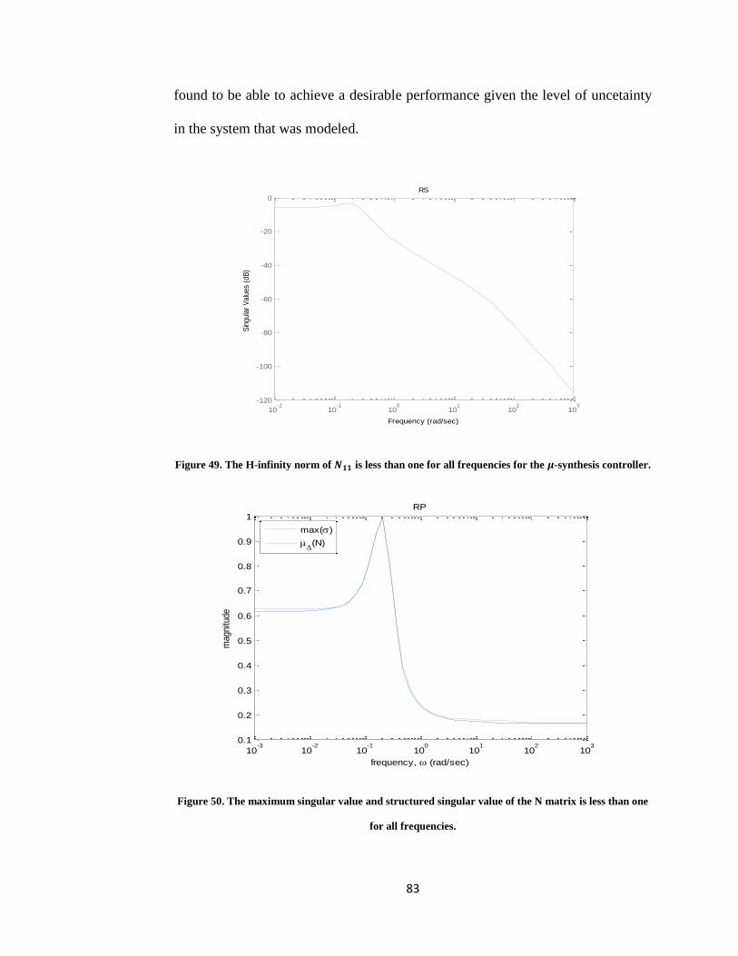
83
found to be able to achieve a desirable performance given the level of uncetainty
in the system that was modeled.
Figure 49. The H-infinity norm of 𝑵𝟏𝟏 is less than one for all frequencies for the 𝝁-synthesis controller.
Figure 50. The maximum singular value and structured singular value of the N matrix is less than one
for all frequencies.
10-2
10-1
100
101
102
103
-120
-100
-80
-60
-40
-20
0
RS
Frequency (rad/sec)
Sin
gula
r V
alu
es (
dB
)
10-3
10-2
10-1
100
101
102
103
0.1
0.2
0.3
0.4
0.5
0.6
0.7
0.8
0.9
1
frequency, (rad/sec)
mag
nitu
de
RP
max()
(N)
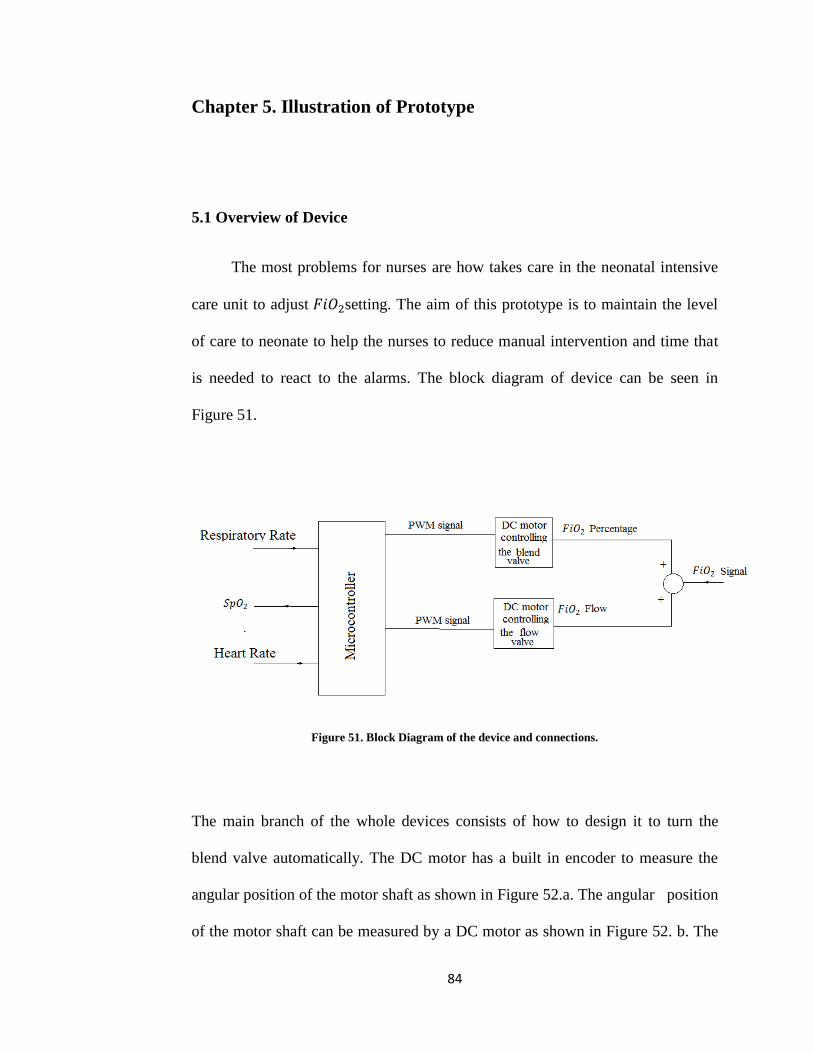
84
Chapter 5. Illustration of Prototype
5.1 Overview of Device
The most problems for nurses are how takes care in the neonatal intensive
care unit to adjust 𝐹𝑖𝑂2setting. The aim of this prototype is to maintain the level
of care to neonate to help the nurses to reduce manual intervention and time that
is needed to react to the alarms. The block diagram of device can be seen in
Figure 51.
Figure 51. Block Diagram of the device and connections.
The main branch of the whole devices consists of how to design it to turn the
blend valve automatically. The DC motor has a built in encoder to measure the
angular position of the motor shaft as shown in Figure 52.a. The angular position
of the motor shaft can be measured by a DC motor as shown in Figure 52. b. The
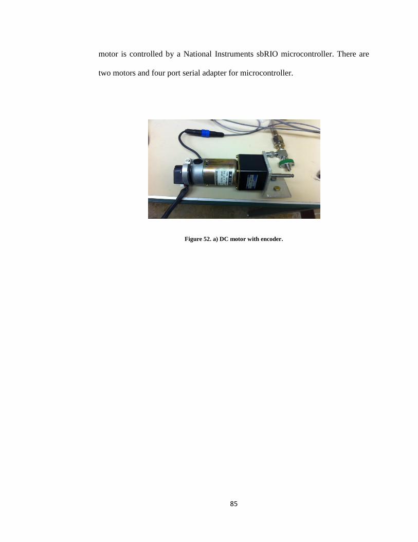
85
motor is controlled by a National Instruments sbRIO microcontroller. There are
two motors and four port serial adapter for microcontroller.
Figure 52. a) DC motor with encoder.

86
(b)
Figure 52. b. Knob tuning device connected to the blend valve knob.
The microcontroller will sample the patient’s vital signs from the port of
Spacelab patient monitor, and these signals will be processed by software
programming that is loaded onto the microcontroller via a laptop that is connected
by link cable. The microcontroller can adjust the value of 𝐹𝑖𝑂2 percentage based
on patient vital signs and we can see the microcontroller in Figure 53.

87
Figure 53. The National Instruments sbRIO microcontroller and power supply.
88
Chapter 6: Conclusion and Signification
6.1. Conclusion of Data
A model for neonatal infants developed by Yu [12] was selected because
there is one input that is 𝐹𝑖𝑂2 and other modes depend on lumped parameter and
non-invasive measurements. The main problem is how we can introduce 𝐹𝑖𝑂2 to
produce 𝑆𝑝𝑂2 between 85% to 93% to keep the infants alive without suffering
from hypoxemia. In this dissertation, we designed PI, PID, MPC, Robust PID, and
Robust MPC controllers to compare between them, which is the best model to
use. The goal is to reduce the amount and spending time of harmful desaturation
for the neonate and to reduce some of the demanding workload of nurses in the
neonatal intensive care unit. The most points that are investigated in this
dissertation are mathematical modeling, identification, controllers, and prototype
instruction.
A nonlinear system model is developed on the system model by Yu [12].
This system model is chosen because it has one input and one output, and does
not require invasive measurements to simulate, the input is 𝐹𝑖𝑂2 for a control
input and output 𝑆𝑝𝑂2 for system model comparison. The linear system model
simulates how the premature infant recovers after a desaturation event. By taking
a first – order Taylor series to linearization and after that we got a linear equation
with one input and one output.
89
In the PI digital controller, we achieved a good response for output without
zero steady state, and the minimum settling time was 180 sec. That needs more
estimated values for 𝐾𝑝 and 𝐾𝐼 after converting the control law from the
continuous domain to the discrete domain by bilinear method. The PI controller
has large overshoots and large steady state error when using large values of 𝐾𝐼 but
when decreasing the values of 𝐾𝐼 got good response with low overshoot and zero
steady.
In the PID controller, we got a good response for output without zero steady
state, and the minimum settling time at 170 sec. that needs more estimated values
for 𝐾𝑝, 𝐾𝐼 and 𝐾𝑑 after converting the control law from the continuous domain to
the discrete domain by bilinear method. The PID controller has large overshoots
and large steady state error when using large values of 𝐾𝐼 and small values of 𝐾𝑝
but when decreasing the values of 𝐾𝐼 and increasing values of 𝐾𝑝 got good
response with low overshoot and zero steady.
The Model Predictive controller was very good in response for 𝑆𝑝𝑂2 with
the input value for control input 21%. MPC needs to be produced first to find the
prediction model, then it must be complete enough to fully capture the process. In
this work, we used the step response produced by DMC to predict the future
response of plant. DMC is a form of control algorithm in which the current
control action is obtained by solving a finite horizon open-loop optimal control.
This process is repeatedly done for each sampling point. The optimization yields
an optimal control sequence, and the first control in this sequence is applied to the

90
plant. The parameters of control horizon and prediction horizon should be kept
short to reduce the computational effort. We took some parameters for prediction
control and the control horizon to see which values are useful for designing. In
general, we concluded that the value of the control horizon should be small to
keep the computational effort manageable, and the value of prediction horizon
should large as possible to completely capture the consequences of the control
action. On the other hand, the weight matrix was very important for the output to
be close to its reference trajectory that we wanted for 𝑝𝑂2. The larger the weight
is for a particular output, the larger is the contribution of its sum of squared
deviations to the objective.
Finally, the manipulated variable that makes the output follow a given trajectory
moves, and the relative magnitude of weight matrix determined the trade - off
between following the trajectory closely and reducing the action of the
manipulated variable. In the result from the design of the MPC, we achieved
𝑆𝑝𝑂2 to be a minimum settling time of 105 sec and zero steady state error.
A robust control system based on the PID controller was introduced to the
plant using the range of parameters found from Bradley Krone’s thesis [30]. For
the robust control system, a nominal model is chosen and perturbations due to
system parameters from this nominal model are used to create a multiplicative
error model. A 𝜇- synthesis controller optimization is used to find a controller
such that the 𝐻∞ norm between the inputs and outputs must be less than one. . We
showed that the result of controller can guarantee stability and performance for
whole range of model parameters. Robust model predictive controller was

91
analyzed, we did get the robust stability, nominal performance and robust
performance. The robust controller is found to have a robust stability and
performance, but with a low bandwidth frequency due to a conservative control
design required to achieve robust stability with an extremely high level of model
error.
In the robust controller with MPC, we estimated modeling for controller in MPC
by RLS and got an accurate response for 𝐹𝑖𝑂2 by supplying error as input to get
modeling. By converting function of the controller from discrete to continuous
and put it as a function in s – domain to use it in robust control. The result we got
was very accuracy with an error model created a 𝜇 - synthesis controller
optimization routine. The main goal of the robust controller was analyzed for
performance and stability. It was shown to be more nominally stable and have
nominal performance and robust stability and performance. We showed that the
result of controller can guarantee stability and performance for a whole range of
model parameters.
We designed a robust control with Model Predictive Control to get a high
accuracy response to be more nominally stable and to have nominal performance
and robust stability and performance. We showed that the result of this controller
can guarantee stability and performance for a whole range of model parameters.
Therefore, the Robust MPC is superior to other controllers because it is more
accurate to prove stability and performance for whole range of model parameters.
92
The robust with PID and robust with MPC control systems are compared to a
static PI, PID, and MPC controllers. The PI and PID digital controller are
designed by using bilinear method and by trial and error. The controllers are
tested using a simulation with varying parameters. The PI controller has large
overshoots and large steady state error when using large values of 𝐾𝐼 but we got
good response with low overshoot and zero steady stare with varying low values
of 𝐾𝐼 but it is less accurate than the robust MPC controller. The PID controller
has low overshoot and zero steady state error with decreasing the values of 𝐾𝐼 and
increasing values of 𝐾𝑝 but we got that with many attempts for trial and error. In
MPC is very accurate with no overshoot and zero steady state, and faster than
using PI and PID. The robust with PID is found to have robust stability and
performance but the robust with MPC is more accurate guarantee stability and
performance for whole range of model parameters.
Future research on controller for arterial saturation in neonatal in infants should
investigate the use of the Robust MPC in more neonates because it has range of
uncertainty and more robust stability and performance to alleviate a load work for
nurses.

93
Appendices
Appendix A: Nomenclature
RDS Respiratory distress syndrome
ROP Retinopathy of prematurity
𝑆𝑝𝑂2 Arterial oxygen saturation
𝐹𝑖𝑂2 Fraction of inspired oxygen
𝑉𝐴 Ventilated part of the lung is perfused with blood
�̇�𝐼 Total respiratory rate
𝑥𝑑 Dead space ratio
𝑉�̇� Respiratory rate of the 𝑉𝐴 section of the lung model
𝑄𝑝 Pulmonary blood flow
𝑄 Total blood flow to respiratory system
𝑃𝐴 The alveolar oxygen partial pressure in the lung
𝐶𝑐 The oxygen content of pulmonary end – capillary blood in vol%
𝐶𝑣 The oxygen content of mixed venous blood in vol%
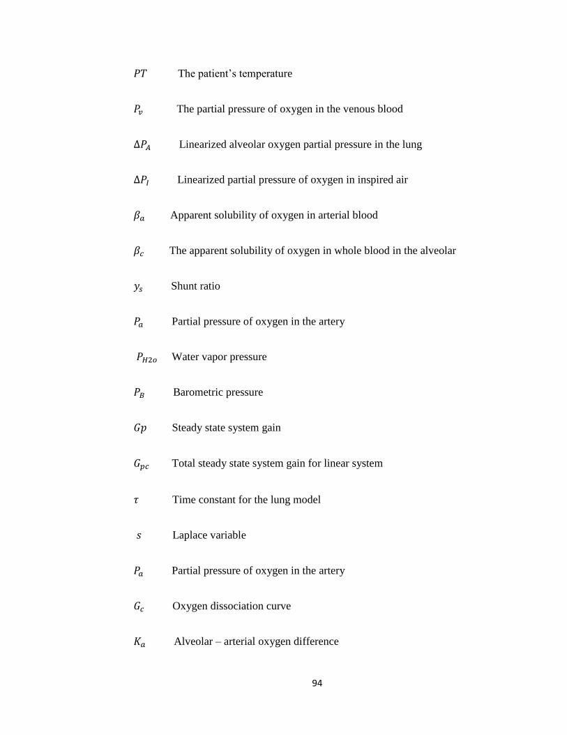
94
𝑃𝑇 The patient’s temperature
𝑃𝑣 The partial pressure of oxygen in the venous blood
∆𝑃𝐴 Linearized alveolar oxygen partial pressure in the lung
∆𝑃𝐼 Linearized partial pressure of oxygen in inspired air
𝛽𝑎 Apparent solubility of oxygen in arterial blood
𝛽𝑐 The apparent solubility of oxygen in whole blood in the alveolar
𝑦𝑠 Shunt ratio
𝑃𝑎 Partial pressure of oxygen in the artery
𝑃𝐻2𝑜 Water vapor pressure
𝑃𝐵 Barometric pressure
𝐺𝑝 Steady state system gain
𝐺𝑝𝑐 Total steady state system gain for linear system
𝜏 Time constant for the lung model
𝑠 Laplace variable
𝑃𝑎 Partial pressure of oxygen in the artery
𝐺𝑐 Oxygen dissociation curve
𝐾𝑎 Alveolar – arterial oxygen difference

95
∆𝑃𝐼 Linearized partial pressure of oxygen in inspired air
𝐾𝑝 Proportional gain
𝐾𝑑 Derivative gain
𝐾𝑖 Integral gain
𝑢(𝑠) The output of controller
𝑧 Z – Transform variable
𝑇 Discrete sampling time
ŷ (𝑡 + 𝑘) Predicted output at future instants
𝑔𝑖 Sampled output values for the step input
∆𝑢(𝑡) Variation of step input
ℎ𝑖 Sampled output
𝐺 System’s dynamic matrix
𝑝 Dimensional vector of the system prediction along the horizon
𝑚 Dimension vector of control increment
𝛤𝑙𝑦
Weighting matrices to penalize particular components of 𝑦
𝛤𝑙𝑢 Weighting matrices to penalize particular components of 𝑢
𝑦(𝑡 + 1) Output predicted over a horizon 𝑝
96
𝑟(𝑘 + 1) Vector of future reference values (set point)
𝐸𝑝(𝑘 + 1|𝑘) Vector of predicted future errors over the horizon 𝑝
𝐾𝑀𝑃𝐶 Stability of the closed – loop system gain
𝑊𝐼(𝑠) Multiplicative uncertainty transfer function weight
𝐺𝑝(𝑗𝜔) Perturbation plant used in error modeling analysis
𝐺𝑛𝑜𝑚(𝑗𝜔) Nominal plant used in error modeling analysis
𝐸𝐼(𝑗𝜔) Multiplicative uncertainty error
𝑤𝑃(𝑠) Error performance weight
𝑤𝑢(𝑠) Control signal performance weight
𝜔𝑏 Bandwidth frequency of the error performance weight
∆ Model uncertainty
∆𝑃 Performance uncertainty
𝐾(𝑠) Robust control
𝑃 Generalized plant matrix
𝑋(𝑡) Output and input matrix
𝜀(𝑡) Error between the true outputs with estimation output
𝜃 ,(𝑡) Estimation output

97
𝑝(𝑡) Auto – correlation matrix
98
References
1. "Neonatal respiratory distress syndrome" at Dorland's Medical Dictionary. 29th
Edition 2012.
2. R.J. Rodriguez, R.J. Martin, and A.A. Fanaroff, “Respiratory distress syndrome and its
management, ”Fanaroff and Martin (eds.) Neonatal-perinatal medicine: Diseases of the
fetus and infant; 7th ed.1001-1011. St. Louis: Mosby 2002.
3. L. Sandra, C. Brian, A. Jacinto, Hemandez, I. Mary, “Merenstein & Gardner’s
handbook of Neonatal Intensive Care” Seventh edition 2010.
4. T. Keim, R. Amjad, and Roger, F., “Modeling and Control of the Oxygen Saturation
in Neonatal Infants,” Dynamic System and Control Conference Arlington, VA, pp. 1-2,
2009.
5. A. Lapttok, W. Salhab, J. Allen, S. Saha, and M. Walsh, “ Pulse Oximetry in Very
Low Birth Weight Infants: Can Oxygen Saturation by Maintained in the Desired
Ranges?,” Perinatol, pp. 337-341, 2006
6. Shyang – Yun Pamela K. Shiao and Ching-Nan Ou “Validation of Oxygen Saturation
Monitoring in Neonates,” American Association of Critical – Care Nurses, 2007
7. L. Roa and I. Ortega-Martinez“ Dynamic analysis of the respiratory system,”
presented at the 19th International IEEE conference, U.S.A.IL, 1997.
99
8. M. Revow, S. England, H. O’beirne, and A. Bryan. “A model of the maturation of
respiratory control in the newborn infant,” in IEEE transaction on Biomedical
Engineering, 1989.
9. F. Tehrani “Mathematical analysis and computer simulation of the respiratory system
in the newborn infant,” in IEEE transaction on Biomedical Engineering, 1993.
10. S. Kanae, K. Muramatsu, Z. Yang and K. Wada, “Modeling of respiration and
estimation of pulmonary elastance,” presented in 5th Asia control conference, 2004.
11. S. Sands, B. Edwards, V. Kelly, M. Davidson, M. Wilkinson and P. Berger “A model
analysis of arterial oxygen desaturation during apnea in preterm infants,” in PLOS
Computational Biology, 2009
12. C.L. Yu, “An Arterial Oxygen Saturation Controller,” Rensselaer Polytechnic
Institute, 1986.
13. L. Zhang, R. Cameron “A Real –Time Expert Control Strategy for Blood Gas
Management in Neonates Under Ventilation Treatment,” Report in Department of
Control Engineering, 1988.
14. F. Tehrani and A. Bazar “An Automatic Control for Oxygen Therapy of Newborn
Infants,” Annual International conference of the IEEE Engineering in Medicine and
Biology Society, 1991.
15. M. Taube and M. Blutani “Automatic Control of Neonatal Fractional Inspired
Oxygen,” Annual International conference of the IEEE Engineering in Medicine and
Biology Society, 1991.
100
16. C. Yu, W. He, J. So, R. Roy and H. Kaufman, “Improvement In Arterial
Oxygen Control Using Multiple Model Adaptive Control Procedures,” in
Department of Biomedical Engineering Rensselear Polytechnic Institute, NY.
17. P. Morozoff, Evans, R., and Smyth, J., “Automatic Control of Blood Oxygen
Saturation in Premature Infants,” presented at the Second IEEE Conference on Control
Applications, Vancouver, B.C., 1993.
18. T. Keim, and F. Roger, “Control of Arterial Oxygen Saturation In Premature Infants,”
Dissertation presented to the Faculty of the Graduated school at the University of
Missouri, 2011.
19. D. Chumlert, W. Anan, and K. Chitsakul, “Automatic Control for Oxygen Intake via
Nasal Cannula,” Proceeding of the International MultiConference of Engineers and
Computer Scientists, 2010.
20N. T. Claure, R. Gerhardt, G. Evert, C. Musante, and E. Bancalari, “Closed – Loop
Controlled Inspired Oxygen Concentration for Mechanically Ventilated Very Low
Weight Infants with Frequent Episodes of Hypoxemia,” official Journal of the American
Academy of Pediatrics, 2001.
21. S. Anand, V. Aswin and S. Kumar, “Simple Tuned Adaptive PI Controller for
Conical Tank Process,” International Conference on Recent Advancements in Electrical,
Electronics and Control Engineering, 2011.
22. R. Youof, S. Omatu and M. Khalid, “Application of Self-Tuning PI Controller to a
Temperature Control System,” published in IEEE, 1994.
101
23. S. Tunyasrirut, J. Ngamwiwit and T. Furuya, “Adaptive Fuzzy PI Controller for
Speed of Separately Excited DC Motor,” Kitakyusbu National College of Technology.
1999.
24. F. Tehrani, “A Control System for Oxygen Therapy Of Premature Infants,”
Proceedings of the 34rd Annual EMBS International Conference, 2001.
25. A. H. Noor, M. Kamal, and F. Yahya, “Application of PID Controller in Controlling
Refrigerator Temperature,” presented at the 5th IEEE International Colloquium on Signal
Processing & Its Application, 2009.
26. M.H. Moradi, “New Techniques for PID Controller Design,” Department of
Electrical Engineering, Iran, 2003.
27. R. Arulmozhiyal and R. Kandiban “Design of Fuzzy PID Controller for Brushless DC
Motor,” International Conference on Computer Communication and Informatics,
Indiana, 2012.
28. J. Taube, R. Pillutla and J. Mills “Criteria For An Adaptive Fractional Inspired
Oxygen Controller,” Drexel University Phospho Engineering, Inc IEEE, 1988.
29. A. Arce, A. Real, and C. Bordons “ Real – Time Implementation Of a Constrained
MPC For Efficient Airflow Control In a PEM Fuel Cell,” in IEEE Transaction on
Industrial Electronics, 2010.
30. K. Bradely, and F. Roger, “Modeling and Control of Arterial Oxygen Saturation in
Premature Infants,” A thesis presented to the faculty of the Graduate school University of
Missouri, 2011.
31. E.F. Camacho and C. Bordons, “Model Predictive Control” 1999, Springer.
102
32. S. Skogestad, I. Postlethwaite, “Multivariable Feedback Control,” John Wiley and
Sons Ltd.: West Sussex, England. P.301-320, 2005
33. J.W. Severinghaus, “Simple Accurate Equations for Human Blood Oxygen
Dissociation Computation,” J.Appl. Phys.:Resp. Environ. Exercise Physiol., 1979.
34. Y.Zhang, G.M. Cui, “Bias compensation models for stochastic systems with colored
noise,” Applied Mathematical Modeling, 2011.
35. Y. Zhang, “Unbiased identification of a class of multi-input single-output systems
with correlated disturbances using bias compensation methods,” Mathematical and
computer Modeling, 2011.
36. F. Ding, Y.J. Liu, B, Bao, “Gradient based and least squares based iterative
estimation algorithms for multi – input systems. Proceedings of the Institution of
Mechanical Engineers,” Part I: Journal of Systems and Control Engineering, 2012.
37. M. Junxia, X. Weili, D. Rui, “Recursive relations of the criterion functions for the
recursive least square algorithms,” In IEEE, 2012.
38. P.E. Wellestead,, and M.B. Zarrop, “Self – Tuning System: Control and signal
processing,”, Johau Wiley and Sous LTD, England 1991.
39. L. JI-Zhen, W. Yong, L. Xiang, “Modeling and Controller Design of Superheated
Steam Temperatures System Based on SVM Combining Adaptive DMC,” IEEE 2007.
103
VITA
Lafta Alkurawy was born in December, 1967 in the city of Baghdad, Iraq. He developed
a genuine interest in engineering in high school, and chose Control and Computer
Engineering as his major at the University of Technology in Baghdad, one of the best
engineering schools in Iraq. He earned his bachelor’s degree in Control and Computer
Engineering from the same of the university. He earned his Master’s degree in Control
Engineering in Electrical and Computer Engineering from the same of the university in
2003. In August 2009, Mr. Lafta Alkurawy moved to the United States and pursued
advanced education at the University of Missouri – Columbia. The following fall, Mr.
Lafta Alkurawy started his doctoral program in the Department of Electrical and
Computer Engineering at the University of Missouri in Columbia.


![Oximetry Refers to determination of percentage of oxygen saturation of the circulating arterial blood. Oxygen saturation= [ HbO 2 ] [HbO 2 ] +[Hb] [ HbO](https://img.dokumen.tips/doc/110x75/56649e9d5503460f94b9dc9f/oximetry-refers-to-determination-of-percentage-of-oxygen-saturation-of-the.jpg)


