Master Thesis Electrical Engineering May 2014

i

Design of an Algorithm for Aircraft Detection and Tracking with a Multi-

coordinate VAUDEO System

Efrén Andrés Estrella Terneux

This thesis is presented as part of Degree of Master of Science in Electrical Engineering

Blekinge Institute of Technology May 2014

Blekinge Institute of Technology School of Engineering Department of Applied Signal Processing Supervisor: Prof. Wlodek J. Kulesza Examiner: Prof. Sven Johansson

ii

This thesis is submitted to the School of Engineering at Blekinge Institute of Technology in partial fulfillment of the requirements for the degree of Master of Science in Electrical Engineering with Emphasis on Signal Processing. The thesis is equivalent to 20 weeks of full time studies.

Contact Information: Author: Efrén Andrés Estrella Terneux Blekinge Institute of Technology Address: SE – 371 79 Karlskrona, Sweden E-mail: andrewsrocks@yahoo.com

Advisors: Prof. Wlodek J. Kulesza School of Engineering, Blekinge Institute of Technology Address: SE – 371 79 Karlskrona, Sweden Phone: +46 455 385898 Email: wlodek.kulesza@bth.se

Dr. Ir. Jelmer Wind Microflown AVISA B.V. Address: Tivolilaan 205 Arnhem, The Netherlands Phone: +31 642004634 Email: wind@microflown.com

iii

Abstract The combination of a video camera with an acoustic vector sensor (AVS) opens new possibilities in environment awareness applications. The goal of this thesis is the design of an algorithm for detection and tracking of low-flying aircraft using a multi-coordinate VAUDEO system. A commercial webcam placed in line with an AVS in a ground array are used to record real low-flying aircraft data at Teuge international airport. Each frame, the algorithm analyzes a matrix of three orthogonal acoustic particle velocity signals and one acoustic pressure signal using the Singular Value Decomposition to estimate the Direction of Arrival, DoA of propeller aircraft sound. The DoA data is then applied to a Kalman filter and its output is used later on to narrow the region of video frame processed. Background subtraction is applied followed by a Gaussian-weighted intensity mask to assign high priority to moving objects which are closer to the sound source estimated position. The output is applied to another Kalman filter to improve the accuracy of the aircraft location estimation. The performance evaluation of the algorithm proved that it is comparable to the performances of state-of-the-art video alone based algorithms. In conclusion, the combination of video and directional audio increases the accuracy of propeller aircraft detection and tracking comparing to reported previous work using audio alone.

Index Terms—Acoustic Vector Sensor, Kalman Filter, Aircraft Tracking, Acoustic Eyes, Acoustic Particle Velocity

iv

v

Acknowledgment This thesis was carried out at Microflown AVISA B.V., Arnhem, The Netherlands, under the supervision of Dr. Ir. Jelmer Wind. Many thanks for his support and patience.

I would like to thank Prof. Wlodek Kulesza for his support and guidance throughout this work. Also special thanks to Dr. Hans Ellias de Bree and Msc. Alex Koers for giving me the opportunity to develop my thesis in a great environment surrounded by the best team of scientists in the field. Thanks to Ivo Diks for his help during measurements day. I would also like to thank Msc. David Pérez Cabo for his happy and knowledgeable support.

vi

vii

Table of Contents

ABSTRACT ......................................................................................................................... iii

ACKNOWLEDGMENT ...................................................................................................... v

TABLE OF CONTENTS ................................................................................................... vii

LIST OF FIGURES ............................................................................................................. ix

LIST OF TABLES ............................................................................................................... xi

LIST OF ABBREVIATIONS ........................................................................................... xiii

1 INTRODUCTION ......................................................................................................... 1

2 BACKGROUND AND RELATED WORK ............................................................... 3

2.1 The Microflown ....................................................................................................... 3

2.2 Aircraft sound localization ....................................................................................... 3

2.3 Aircraft tracking on video ........................................................................................ 5

2.4 VAUDEO sensor fusion .......................................................................................... 6

2.4.1 Sensor fusion principles ..................................................................................... 6

2.4.2 Coordinate system transformation ...................................................................... 6

3 PROBLEM STATEMENT .......................................................................................... 7

4 AIRCRAFT TRACKING IN REAL-TIME VIDEO ............................................... 11

4.1 Video camera model .............................................................................................. 11

4.2 Aircraft motion detection ....................................................................................... 13

4.2.1 Background subtraction algorithm ................................................................... 14

4.2.2 Data validation .................................................................................................. 15

4.3 Kalman filter target tracking .................................................................................. 15

5 ACOUSTIC AIRCRAFT TRACKING ..................................................................... 19

5.1 Sound acquisition ................................................................................................... 19

5.2 Pre-processing, detection and classification .......................................................... 20

5.3 DOA estimation ..................................................................................................... 20

5.4 Coordinates transformation .................................................................................... 21

5.5 Kalman tracking of sound source .......................................................................... 21

5.6 Screen-to-display coordinates mapping ................................................................. 23

5.7 Distance to the aircraft estimation ......................................................................... 23

viii

6 METHOD VALIDATION AND PERFORMANCE EVALUATION ................... 27

6.1 Measured low-flying aircraft data .......................................................................... 27

6.2 Performance Evaluation ......................................................................................... 29

6.2.1 Reference Annotation ....................................................................................... 30

6.2.2 Performance Measures - Euclidean distance and MODA ................................ 30

6.3 Real-time MATLAB Demonstration ..................................................................... 34

6.4 Discussion .............................................................................................................. 34

7 CONCLUSIONS AND FURTHER WORK ............................................................. 37

7.1 Single-node VAUDEO System ............................................................................. 37

7.2 Further Work .......................................................................................................... 38

7.2.1 Distributed VAUDEO system .......................................................................... 38

7.2.2 Aircraft range estimation .................................................................................. 38

REFERENCES ................................................................................................................... 39

APPENDIX A ...................................................................................................................... 41

A.1 Calibration Procedure .................................................................................................... 41

ix

List of Figures

Figure 1 The acoustic-vector sensor developed by Microflown®. ........................................ 3 Figure 2 Airborne vehicle localization using triangulation[1] ............................................... 4 Figure 3 Background subtraction diagram ............................................................................. 5 Figure 4 Sensor fusion ............................................................................................................ 6 Figure 5 Audio and video coordinate systems ....................................................................... 7 Figure 6 VAUDEO tracking algorithm .................................................................................. 8 Figure 7 Geometric model of the camera ............................................................................. 12 Figure 8 Aircraft tracking on video block diagram .............................................................. 13 Figure 9 Background subtraction steps. a) Current frame. b) Previous frame. c) Frame differencing. d) Threshold applied. ...................................................................................... 14 Figure 10 Gaussian ROI ....................................................................................................... 15 Figure 11 Block diagram of the acoustic tracking algorithm ............................................... 19 Figure 12 Camera, screen and raster coordinate systems ..................................................... 21 Figure 13 VAUDEO aircraft tracking with distance estimation. ......................................... 24 Figure 14 Distance to the aircraft estimation (simple case) ................................................. 24 Figure 15 VAUDEO prototype............................................................................................. 28 Figure 16 VAUDEO output .................................................................................................. 28 Figure 17 Frame annotations for low-flying aircraft in VAUDEO ...................................... 30 Figure 18 Euclidean distance per frame ............................................................................... 31 Figure 19 Localization errors per aircraft ............................................................................. 32 Figure 20 Percentiles for the all dataset................................................................................ 33 Figure 21 N-MODA boxplot ................................................................................................ 34 Figure 22 Screenshot of the real-time MATLAB demonstration. ........................................ 35 Figure 23 Calibration points in the video camera frame. ..................................................... 43

x

xi

List of Tables TABLE 4.1 Video camera specification ....................................................................................... 11 TABLE 4.2 Discrete-time linear Kalman filter ............................................................................. 17 TABLE 6.1 Specification of the AVS used for the experiment ..................................................... 29 TABLE 6.2 Experimental VAUDEO data collection .................................................................... 29

xii

xiii

List of Abbreviations

AVS - acoustic vector sensor

CEP - circular error probable

DoA - direction of arrival

RADAR – radio detection and ranging

SVD - singular value decomposition

VAUDEO – video + audio combination

xiv

1

1 Introduction

Airborne sound source detection and tracking is becoming a necessity in order to provide environment awareness and security to people, equipment and facilities in cities and battlefields. Current widespread technologies used to detect and track aircraft are based on RADAR. They possess a well know disadvantage which is the blind zone through which small aircraft can fly undetected close to the ground. This vulnerability has been exploited for illegal activities, and could potentially be used for terrorists attacks, spy drones, etc. Therefore, it is desirable to complement RADAR by using acoustic vector sensors (AVS) in combination with a camera for detection and tracking of low-flying fixed-wing aircraft.

Many other potential applications are envisioned using Microflown’s technology since virtually any airborne sound source could be located and tracked within a range which is usually difficult to cover when using only traditional technologies like RADAR. The airborne sound source considered in this thesis is limited to a low-flying fixed-wing aircraft. However, other types of airborne vehicles like helicopters can also be located with further work. Surveillance applications as well as security and defense sectors could benefit greatly by using VAUDEO (Video-audio combination) enabled equipment.

The idea to detect and track low-flying aircraft using acoustic-vector sensors have been presented first in [1], and was subsequently followed by a proof of concept in [2] in which a video camera was added to the task. It was observed an unreliable estimation of the elevation of the airborne sound source using only AVSs and no real world aircraft data was considered for the proof of concept. It was required to continue the development of the prototype with measurements in a real world environment, and solve the challenge of VAUDEO combination in a generic way.

This thesis contributes to Microflown’s aim to develop high-tech surveillance tools complementary to existent technologies. Accordingly, the purpose of this thesis is to design and test an algorithm for low-flying aircraft detection and tracking using a VAUDEO system. One video camera is placed in combination with a 3D AVS; a calibration procedure is developed, and with help of various image and audio processing techniques the system can determine the position and track an aircraft flying low in space. The presented solution is not computationally expensive and can be implemented in embedded systems without special requirements.

The present thesis consists of 7 chapters. The first one is an introduction to the problem considered in the thesis. Chapter 2 is a survey of related work and background data followed by the problem statement in chapter 3. Chapter 4 and 5 describes the design of aircraft tracking algorithms from a real-time video perspective and an AVS perspective respectively. Chapter 6 is devoted to performance evaluation of the prototype and method validation. The last chapter summarizes the results obtained in the thesis and lists future work.

2

3

2 Background and Related Work

2.1 The Microflown The Microflown is a sensor which can measure true acoustic particle velocity in a small spot. The sensor principle is based on the measurement of the electric resistance difference between two 200 [nm] thick platinum wires, which are placed closely and heated to about 300 [°C]. When acoustic particle velocity is present the temperature difference between the wires changes, which in consequence changes their electrical resistance due to thermal resistance effect. The sensor output voltage is therefore proportional to the acoustic particle velocity, and its responsivity is frequency dependent [3].

The probe used for this thesis is an acoustic vector sensor (AVS) which encloses three orthogonally placed microflowns plus one pressure microphone as can be observed in Figure 1. With this calibrated probe the sound intensity in 3D can be measured.

Figure 1 The 3D acoustic-vector sensor developed by Microflown®

2.2 Aircraft sound localization Traditional sound source localization techniques rely on an estimation of Time Difference of Arrival (TDOA) at microphone arrays through GCC-PHAT and beam-forming methods [4]. This thesis approaches the aircraft sound localization system in a different manner using an AVS developed by Microflown Technologies [5]. Therefore, relevant research comprises the discipline of sound source localization using acoustic-vector sensors. Many references can be cited; a few are reviewed here.

A theoretical method for localization of sound sources using a vectorial approach was proposed first by Nehorai in [6]. The same year the Microflown was discovered, and the

4

AVS in Figure 1, which consists of two or three acoustic particle velocity sensors and a sound pressure transducer, was subsequently developed [5][7]. Following this development several algorithms appeared which enable the localization of sound sources based on the estimation of the sound intensity vector at the sensing point. A summary of the most relevant applications can be found in [3].

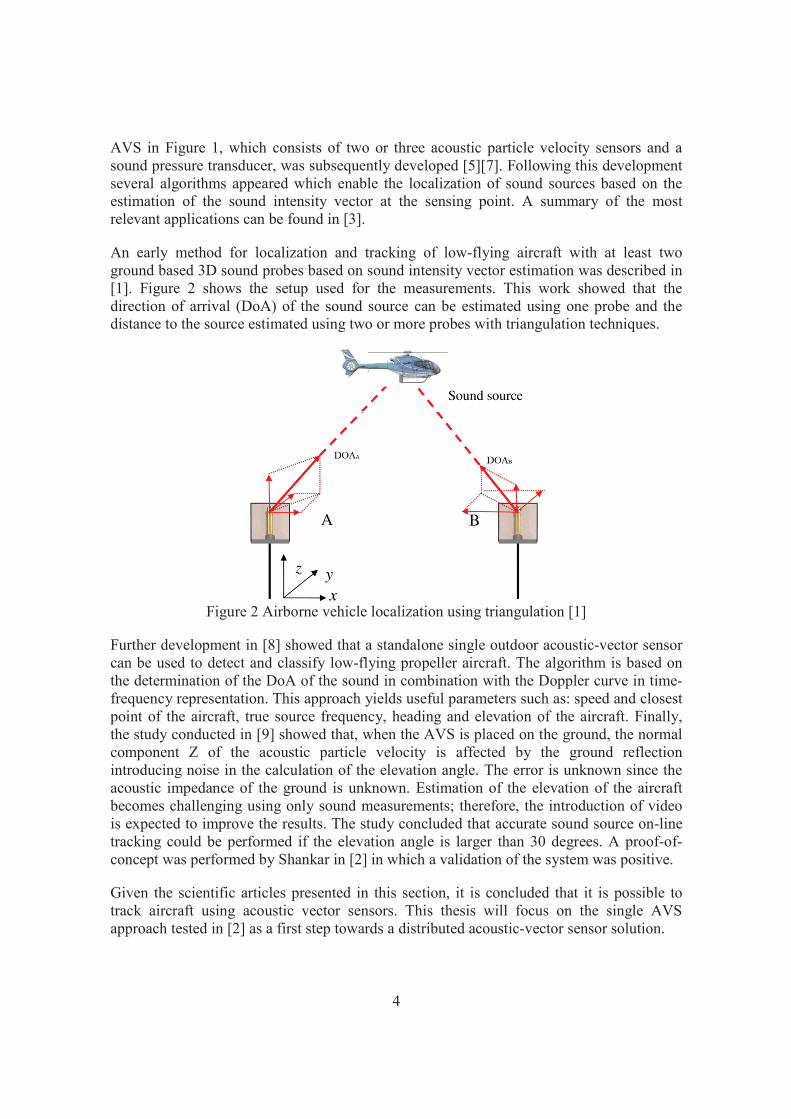
An early method for localization and tracking of low-flying aircraft with at least two ground based 3D sound probes based on sound intensity vector estimation was described in [1]. Figure 2 shows the setup used for the measurements. This work showed that the direction of arrival (DoA) of the sound source can be estimated using one probe and the distance to the source estimated using two or more probes with triangulation techniques.

Figure 2 Airborne vehicle localization using triangulation [1]

Further development in [8] showed that a standalone single outdoor acoustic-vector sensor can be used to detect and classify low-flying propeller aircraft. The algorithm is based on the determination of the DoA of the sound in combination with the Doppler curve in time-frequency representation. This approach yields useful parameters such as: speed and closest point of the aircraft, true source frequency, heading and elevation of the aircraft. Finally, the study conducted in [9] showed that, when the AVS is placed on the ground, the normal component Z of the acoustic particle velocity is affected by the ground reflection introducing noise in the calculation of the elevation angle. The error is unknown since the acoustic impedance of the ground is unknown. Estimation of the elevation of the aircraft becomes challenging using only sound measurements; therefore, the introduction of video is expected to improve the results. The study concluded that accurate sound source on-line tracking could be performed if the elevation angle is larger than 30 degrees. A proof-of-concept was performed by Shankar in [2] in which a validation of the system was positive.

Given the scientific articles presented in this section, it is concluded that it is possible to track aircraft using acoustic vector sensors. This thesis will focus on the single AVS approach tested in [2] as a first step towards a distributed acoustic-vector sensor solution.

5

2.3 Aircraft tracking on video One of the main motivating factors of this work has been the potential to improve the localization of a sound emitting source using video and audio. This work presents an algorithm for localization of moving objects on a video sequence using a priori audio information. Also, the possibility to estimate the distance to the moving object is explored by exploiting the fact that sound travels slower than light. Some relevant research on motion detection techniques as well as tracking of objects on video is summarized here.

Cheung et al. [10] have presented a comparison between different background subtraction techniques in urban environment ranging from simple methods such as frame differencing to more complex probabilistic models. In the aircraft motion detection algorithm a frame differencing technique for background modeling is chosen as the first step. Since real-time processing is required, this technique offers a good trade-off between low computational requirements and good motion detection.

In a previous work by Shankar [2], a background subtraction approach was proposed for aircraft motion detection. This method proved to perform well on ideal conditions, but not in presence of noise or other moving objects in the field-of-view (FOV). A general flow diagram of the algorithm is shown in Figure 3. Some modifications to this algorithm are introduced in order to improve the localization as shown in chapter 4.

Figure 3 Background subtraction diagram

Several methods for tracking moving objects on real-time video have been proposed over the last decades. For instance, Gilbert et al. [11] described the theoretical aspects of an early “intelligent” airborne-target tracking system using a videotheodolite and a finite-state-machine. Bourqui [12] applied a Kalman filter approach to track objects in a highway environment video. Later, Jang [13] utilized Kalman filtering to predict motion information of a moving target and effectively reduce the search space using a region-of-interest ROI. In the present work, tracking and velocity estimation of the aircraft is performed using a Kalman filter using information from both AVS and video camera.

6

2.4 VAUDEO sensor fusion 2.4.1 Sensor fusion principles

“Sensor fusion is the combination of sensory data or data derived from sensory data in order to produce enhanced data in form of an internal representation of the process environment. The achievements of sensor fusion are robustness, extended spatial and temporal coverage, increased confidence, reduced ambiguity and uncertainty, and improved resolution” [14]. The VAUDEO concept involves the combination of observations from two different sources into a coherent description of the observed event. In this case the location estimation of a propeller aircraft. The general framework of the fusion is shown in Figure 4.

Figure 4 Sensor fusion

2.4.2 Coordinate system transformation In order to combine data gathered from sensors measuring different physical quantities of the same phenomenon, first it is necessary to have both measurements relative to a common coordinate system. Specifically, it is necessary to convert the points in audio coordinates to video coordinates before performing sensor fusion. The problem of matching points within different coordinate systems has been studied in different applications. For instance, in [15] Hanson and Norris derived an algorithm based on the assumption that the relation between two sets of coordinates is a certain rigid transformation. Their solution is related to the solution of the Procrustes problem by Schönemann [16].

Also, in [17] the authors proposed a sensor calibration procedure in order to convert points from image coordinates to airport map coordinates assuming that the points are related by a homography [18], which defines a relation between two images of the same planar surface in space. The approach used on this thesis is to transform points from audio coordinates to video coordinates using a linear transformation matrix found through calibration and the least squares solution of the resultant over-determined equation system. Details of the calculations are presented in chapters 4 and 5.

7

3 Problem Statement

The combination of video and audio tracking opens up a range of possibilities which are practically impossible using audio or video alone. An aircraft passive tracking system complementary to RADAR is one possibility and, it is attractive since it does not emit energy and can cover blind-zones. Acoustic vector sensors (AVS) enable the development of a system for passive tracking of propeller airplanes. The approach tested in [9] showed that an acoustic tracking system is feasible using two PU probes and triangulation. However, unreliable estimation of the direction of arrival (DoA) in spherical coordinates for elevation of the sound source below 30 degrees was observed. To overcome this limitation, the combination of a video camera with an AVS is going to be investigated. An accurate estimation of the position of the aircraft is expected from the VAUDEO combination as well as passive tracking of the object. An algorithm combining information from two different coordinate systems for detection and tracking of an aircraft is proposed.

To define the problem, some assumptions and requirements are established. First, the x-axis of the AVS needs to be aligned with the optical axis1 of the camera, and the coordinate system XYZ is a linear transformation of X’Y’Z’ as shown on Figure 5. The diagonal field-of-view (FOV) of the camera is 74°, and the necessary resolution is 640x480 pixels in RBG color. Second, 4-channel audio is sampled at 44100 [Hz] with 16 bits using a USB external sound card. Three-channel particle velocity is measured in orthogonal directions and one-channel sound pressure.

One challenge is mapping the DoA of the sound source from the AVS coordinate system to a point in the camera view. In other words, being able to track on video feeds the aircraft with aid of its sound. The first research question is: how to track low-flying aircraft accurately and reliably based on audio and video data? The auxiliary research question is: How to calibrate such system? The second research question is: how to estimate the distance between the sensors and the aircraft using VAUDEO sensor fusion?

Figure 5 Audio and video coordinate systems

1 It's the line from the apex of the pyramid to the center of the base.

8

Figure 6 VAUDEO tracking algorithm

To answer these questions it was assumed that the transformation from a point in the AVS coordinate system to the camera coordinate system is an affine transformation. In that way the problems are: finding a transformation matrix between points in both coordinate systems, and defining a suitable algorithm for VAUDEO aircraft tracking. The distance to the aircraft can be estimated using the time delay of the sound position with respect to video.

The proposed tracking algorithm is improved from the one presented in [2], and its flowchart is shown in Figure 6. The algorithm consists of 4 main parts; each one performing a specific task. First, an audio detection algorithm detects the presence of a tonal sound source and, a classification algorithm defines if it is an aircraft, helicopter, etc. Subsequently, audio localization is performed and the DoA of the source extracted. Once the aircraft reaches the FOV of the video camera, a VAUDEO tracking algorithm takes

9

over. The position and velocity of the aircraft in spherical coordinates can be estimated at this stage as it will be shown in the following chapters.

The main contribution of this thesis is a conceptual solution that takes into consideration previous work in the area as well as a new approach to link directional audio and video in a common statistical framework. A calibration procedure to map the sound source DoA in 3D space to a video frame is designed and tested. In order to test the algorithms, a fully functional prototype able to record data and process off-line and on real-time is implemented in MATLAB. The proposed solution has been validated, and the prototype experimentally verified.

10

11

4 Aircraft tracking in real-time video

The first task in understanding how a video camera can be used as a sensing device is in defining its geometrical model. With enough understanding of the geometrical model, the aircraft video tracking system can be simplified to tracking a point moving in a 2-D surface i.e. the video display. In the next section the aircraft tracking algorithm on video is detailed. If the response of the real system matches the model correctly, then it is possible to be confident about the results and actions taken to improve the system performance.

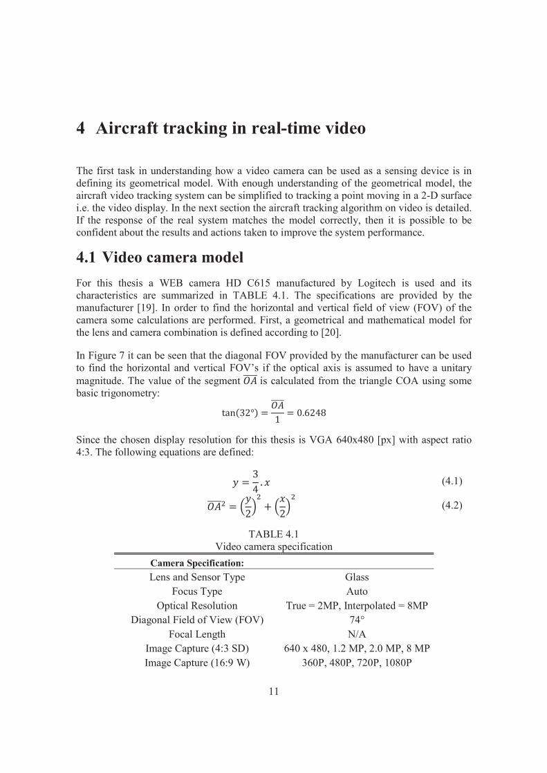
4.1 Video camera model For this thesis a WEB camera HD C615 manufactured by Logitech is used and its characteristics are summarized in TABLE 4.1. The specifications are provided by the manufacturer [19]. In order to find the horizontal and vertical field of view (FOV) of the camera some calculations are performed. First, a geometrical and mathematical model for the lens and camera combination is defined according to [20].

In Figure 7 it can be seen that the diagonal FOV provided by the manufacturer can be used to find the horizontal and vertical FOV’s if the optical axis is assumed to have a unitary magnitude. The value of the segment is calculated from the triangle COA using some basic trigonometry:

Since the chosen display resolution for this thesis is VGA 640x480 [px] with aspect ratio 4:3. The following equations are defined:

(4.1)

(4.2)

TABLE 4.1 Video camera specification

Camera Specification: Lens and Sensor Type Glass

Focus Type Auto Optical Resolution True = 2MP, Interpolated = 8MP

Diagonal Field of View (FOV) 74° Focal Length N/A

Image Capture (4:3 SD) 640 x 480, 1.2 MP, 2.0 MP, 8 MPImage Capture (16:9 W) 360P, 480P, 720P, 1080P

12

Video Capture (4:3 SD) 320 x 240, 640 x 480 Video Capture (16:9 W) 360P, 480P, 720P, 1080P

Frame Rate (max) 30 FPS @640 x 480

Figure 7 Geometric model of the camera

Replacing (4.1) in (4.2) and solving for x yields:

(4.3)

The values of the angles α and β in Figure 7 can be calculated in order to find the horizontal and vertical FOV’s using trigonometry according to:

Yields,

13

HFOV = 2α = 53.1301 [°]

VFOV = 2β = 41.1121 [°]

With the calculated values the frustum in which the aircraft can be observed by the camera is defined, and the equivalence angle-pixel for a unitary optical axis is found according to:

, Azimuth (4.4)

, Elevation (4.5)

4.2 Aircraft motion detection In order to track low-flying aircraft on video, the algorithm of Figure 8 is proposed. It introduces some modifications to the algorithm used in [2] by Shankar; for instance, the frame-rate of the camera is increased to 10 [FPS], and a region-of-interest (ROI) based on audio is utilized to narrow the search space. A Kalman filter for tracking and parameter estimation is also added. The following subsections describe the methods and techniques applied.

Figure 8 Aircraft tracking on video block diagram

14

Figure 9 Background subtraction steps. a) Current frame. b) Previous frame. c) Frame differencing. d) Threshold applied.

4.2.1 Background subtraction algorithm

The first step in object motion detection is to extract a background frame for background subtraction. When the aircraft trajectory reaches the FOV of the camera, the first two frames are used as background frame and foreground frame respectively. The frames are then converted from RGB to grayscale since the algorithm handles luminance intensity of each pixel. The next step is the application of a frame differencing [10] technique which was successfully used for background modeling. It was chosen because of its simplicity and robustness when combined with information from directional audio. Frame differencing basically uses the video frame at time (t - 1) as background model for the frame at time t. The result of this process is presented in Figure 9c.

The third step in motion detection is foreground detection. In this work, the differenced frames are compared against a threshold according to:

(4.6)

Where It and Bt are pixel intensities on the current and background frames respectively. T is the threshold determined experimentally. Figure 9d shows the foreground frame after threshold.

15

4.2.2 Data validation

Data validation is the process of improving the candidate foreground mask [10]. If audio tracking information is available, it can be used to define a region-of-interest (ROI) to search for the aircraft. In this work, the ROI is defined as a rectangular area centered in the estimated audio position with the intensity values following a Gaussian distribution. This approach enables the algorithm to emphasize the pixels which are close to the sound source while removing the pixels which are not related to the sound source. Figure 10 shows the Gaussian mask for ROI in a) and the resultant foreground mask in b).

Figure 10 Gaussian ROI

4.3 Kalman filter target tracking Once the foreground mask is obtained, the coordinates of the centroid of the biggest “blob” are calculated and tracked. The coordinates in pixels (x,y) are the location estimation of the aircraft. Kalman filtering is applied for target tracking in order to obtain accurate location and velocity estimates of the aircraft. A continuous-time state-space model of the aircraft is introduced according to [21]:

(4.7) (4.8)

16

where w(t) v(t) are zero-mean Gaussian white noise processes with covariance given according to:

(4.9) (4.10) (4.11)

In this thesis, a kinematic model is used to derive the estate estimate which involves the aircraft’s position and velocity on x and y coordinates. The truth model in continuous time is defined as:

(4.12)

where the process noise is w(t) = [wx(t) wy(t)]T with spectral density q, and the states are the position and velocity of the aircraft on the screen in pixels

and pixels per second.

Measurements of position are in discrete-time and are modeled according to:

(4.13)

where vk is the measurement noise, which is modeled by zero-mean Gaussian white-noise processes with variance σx

2 and σy2.

The Kalman filter for video points uses a discrete-time model that is derived from the model in equation (4.12) according to [21]. First, the discrete-time state transition matrix is calculated for F constant and F2 = 0. It yields,

(4.14)

where = 0.1 [s] is the sampling interval. The next step is the determination of the discrete-time process noise covariance. The matrix is determined by solving the following integral:

(4.15)

replacing G, Q and in (4.15) yields,

(4.16)

If it is assumed that qx = qy =q, then, evaluating the integral results in:

17

(4.17)

Finally, the discrete-time linear Kalman filter equations for video coordinates are used according to TABLE 4.2.

TABLE 4.2 Discrete-time linear Kalman filter

Model

Initialization

Gain

Update

Propagation

where is the state-transition matrix, the observation matrix, and vk and wk are assumed to be zero-mean Gaussian white-noise processes.

18

19

5 Acoustic aircraft tracking

In the previous chapter, tracking of aircraft was considered using video. The next task is to develop an algorithm for aircraft tracking using its sound. This chapter introduces sound source localization using the AVS developed by Microflown®. This chapter starts by presenting a block diagram in Figure 11 of the acoustic tracking algorithm while the remaining sections explain each block. A brief discussion is presented in the end.

Figure 11 Block diagram of the acoustic tracking algorithm

5.1 Sound acquisition In this thesis the algorithms are implemented and evaluated on a personal computer equipped with a multi-channel sound card. The sampling frequency is set to 44100 [Hz] and quantization is performed using 16 [bits]. Four channels were used, one for sound

20

pressure and three for the components of acoustic particle velocity. The acquisition of sound is performed in sequential batches of 4410 [samples] each, or 0.1 [s] of raw data per batch.

5.2 Pre-processing, detection and classification In order to determine the DoA of aircraft sound it is necessary first to detect its presence on the vicinity. Detection and classification of aircraft sound is approached by using the algorithm based on Page’s test [22] for detecting trends in data and image processing techniques described in [2]. No major modifications are introduced to the algorithm, although the detection parameters are adjusted for real propeller aircraft sound. This step is important since it enables the tracking algorithms to perform their task while an aircraft is present, and to enter stand-by mode otherwise. Also, detection is used to trigger logging of raw VAUDEO signals if necessary.

5.3 DoA estimation Direction-of-arrival estimation of far-field acoustic signals is necessary when localizing a moving sound source. Several methods exist for arrays of microphones; however, if acoustic particle velocity is added to DoA estimation, a different approach is required.

In this thesis, DoA estimation is performed using a proprietary algorithm. First, a matrix of data ANx4 is formed by placing on the first column a vector of N sound pressure samples, and 3 vectors of N orthogonal particle velocity samples on the next columns. N is the window size and its value is determined empirically. Matrix A is then factorized using the singular value decomposition (SVD) according to:

,

.

where σ are the singular values of A, and V contain the principal components of the sampled data i.e. orthonormal vectors pointing in the direction of highest variance.

A unitary vector pointing in the direction of highest energy yields in vector v1. In this specific case: v1= [p1 vx1 vy1 vz1] where p1 gives the sign of the acoustic particle velocity vector and vx1, vy1, vz1 its components. The DoA is estimated according to:

,

since it points in the opposite direction of the acoustic particle velocity vector. It can be shown that this procedure is equivalent to conventional beam-forming for the case when only one AVS is used.

21

5.4 Coordinates transformation The DoA estimated in the preceding section is relative to the coordinate system spanned by the AVS. In order to visualize the DoA in the screen, a coordinate system transformation is necessary.

The transformation is assumed affine, and it is performed by multiplying the DoA unitary vector with a transformation matrix T previously determined by calibration. The calibration procedure is detailed in Appendix A. The resulting DoA vector is relative to the axis X’Y’Z’ in Figure 12 which shows the camera, screen and display coordinate systems.

Figure 12 Camera, screen and raster coordinate systems

5.5 Kalman tracking of sound source The components of the resultant DoA vector are contaminated with physical noise from the sensory system, round-off errors and other unpredictable phenomena. It becomes necessary the utilization of some form of optimal filtering to get an accurate DoA vector estimate. It is also important to use a-priori information about the target attitude. The Kalman filter is appropriate for this task since it can filter Gaussian distributed noise while keeping a dynamic model of the aircraft and the noise.

22

The same continuous-time state-space model of the aircraft introduced in equations (4.7)-(4.11) is used. The “truth” model in continuous time is defined as:

(5.1)

where the process noise is w(t) = [wx(t) wy(t) wz(t)]T with spectral density q, and the states are the position and velocity of the aircraft on each of

the orthogonal components X’Y’Z’ of its DoA vector.

Measurements of DoA components are in discrete-time and are modeled according to:

(5.2)

where vk is the measurement noise, which is modeled by zero-mean Gaussian white-noise processes with variance σx

2, σy2 and σz

2.

The Kalman filter for audio points uses a dicrete-time model that is derived from the model in equation (5.1) according to [20]. First, the discrete-time state transition matrix is calculated for F constant and F2 = 0. It yields,

(5.3)

where = 0.1 [s] is the sampling interval. The next step is the determination of the discrete-time process noise covariance. The matrix is found solving the following integral:

(5.4)

replacing G, Q and in (5.4) and solving the integral yields,

(5.5)

23

The discrete-time linear Kalman filter equations for sound coordinates are used according to TABLE 4.2. The filtered components are the DoA estimation of the sound emitted by the aircraft while low-flying.

5.6 Screen-to-display coordinates mapping An equivalence of points in X’Y’Z’ coordinates to pixels in display coordinates is required, and it is obtained as follows. First, the DoA vector is transformed to spherical coordinates, and the angles of azimuth and elevation are used with (4.4) and (4.5) in order to obtain screen coordinates. For instance, a unitary vector is defined as = [θ,φ,1]T in spherical coordinates. Its screen coordinates are calculated according to:

(5.6)

(5.7)

where and . Since the display coordinates can have only integer values (pixels), it is required to round-off the screen coordinates and perform an origin translation with 180° rotation as shown in Figure 12. The estimated display coordinates of the moving sound emitting source have a resolution of 640x480 pixels.

5.7 Distance to the aircraft estimation The distance from the sensors’ origin to the aircraft can be estimated by exploiting the fact that light travels faster than sound in air. A sensors fusion approach is utilized.

As it can be observed in Figure 13, the estimated position of the aircraft sound closely follows the video estimated position. The value of x contains information about the distance that sound travelled to reach the sensors.

24

Figure 13 VAUDEO aircraft tracking with distance estimation.

Figure 14 Distance to the aircraft estimation (simple case)

In Figure 14 a simple case is analyzed. First, two equations are defined:

(5.8) (t) t (5.9)

where Pa and Pv are the position of the aircraft at time t according to audio and video respectively, is the velocity of the aircraft and t is the time sound takes to travel from the aircraft to the sensors, and is equivalent to the time Pa takes to reach Pv in display coordinates. It is assumed that the velocity of the aircraft remains constant during the considered interval t. Replacing (5.9) in (5.8) yields:

25

(t) t (5.10)

It is observed in equation (5.10) that the terms in the left side equal x. is equal to where d is the distance to the source and c is the acoustic wave propagation

speed. Replacing and solving for the distance d, the following formula is obtained.

(5.11)

The value of is estimated in [pixels/s] in the state-variable of the Kalman filter used for video tracking. The speed of sound is chosen according to the altitude and temperature of the environment.

26

27

6 Method Validation and Performance Evaluation

A VAUDEO prototype was used to collect data in an experiment at Teuge International airport. A picture of the arrangement can be seen in Figure 15. In this chapter, empirical data is analyzed; the output response from the prototype is shown, and its performance evaluated using the framework described in [22]. A real-time output demonstration in MATLAB is presented.

6.1 Measured low-flying aircraft data In order to validate the proposed algorithm, two experiments were conducted. The experiments were performed at Teuge International airport in The Netherlands during daytime. The specification of the equipment used for the experiments can be referred in TABLE 4.1 and TABLE 6.1. The VAUDEO prototype was placed at 275 [m] from the aircrafts route. All samples were captured with noise in a real environment. The frame rate of the camera is set to 10 [fps] while the audio is sampled at 44100 [Hz] with 16 [bits] of resolution.

First, 4 clips with 4 aircraft flying low were recorded in order to train the system. The ambient temperature was 4° [C]. For testing, 11 clips were recorded with ambient temperature of 18° [C]. The experimental VAUDEO data collection can be observed in TABLE 6.2

Experimental VAUDEO data collection. Since the speed of sound is proportional to ambient temperature, temperature is registered in order to estimate the distance at which the sound source is located accurately.

28

Figure 15 VAUDEO prototype

For every audio clip, it was discretely segmented into 100 [ms] frames in correspondence with the frame rate of the camera. That is, 100 [ms] of audio data per each video frame. Then, each VAUDEO clip is analyzed frame by frame with MATLAB.

An example of VAUDEO output when tracking an aircraft flying low is shown in Figure 16. The red marker shows the position of the aircraft estimated using VAUDEO while the blue marker shows the position of the aircraft estimated using only its propeller sound.

Figure 16 VAUDEO output

29

TABLE 6.1 Specification of the AVS used for the experiment

AVS Specification:

Sensor Configuration 3x uflown Titan sensor 1x Knowles FG pressure mic.

Microphone element Frequency Range 20 – 20k [Hz] Upper sound level 110 [dB]

Polar pattern Omnidirectional Directivity Omnidirectional

Microflown element Frequency range 0.1 -20k [Hz] +- 1 [dB]

Upper sound level 135 [dB] Polar pattern Figure of eight Directivity Directive

TABLE 6.2 Experimental VAUDEO data collection

Total clips Template clips Testing clips Total frames Fixed-wing aircraft 15 4 11 630

Ambient 2 1 1 21400

In order to test the performance of the algorithm it is necessary to analyze the data and define which of the events are valid. Aircraft are either landing or taking off. Since a fixed-wing aircraft hardly emit audible sound during landing, those are omitted. Also, the evaluation performed on this thesis is limited to the case where there is only one plane flying at one time. Finally, cases where the aircraft is occluded are not included and will be considered in future work.

6.2 Performance Evaluation The measured data enabled the system to achieve accurate localization and tracking of the low-flying aircraft. A VAUDEO aircraft detection and tracking task could be defined as spatially detecting an aircraft with a-priori audio information on each individual frame and linking it on sub-sequent frames while the aircraft is present on the FOV of the camera. To evaluate the performance of the proposed algorithm, the framework in Kasturi et al. [23] was applied with little modification. First, a set of ground-truth was hand-annotated and validated. Then, the Euclidean distance in pixels between points on the ground-truth and the estimated aircraft’s position (prototype’s output) is calculated per each frame for the whole dataset. With help of the development in section 4.1, the Euclidean distance in pixels can be expressed in degrees. Finally the results are discussed.

30

6.2.1 Reference Annotation

The video sequence was hand-annotated using the Video Performance Evaluation Resource (ViPER) [24] in order to produce ground-truth for evaluation. The annotation of the VAUDEO sequence was done following the guidelines stated in [23]. Each aircraft was marked by a non-oriented bounding box with its centroid as shown in Figure 17.

Figure 17 Frame annotations for low-flying aircraft in VAUDEO

6.2.2 Performance Measures - Euclidean distance and MODA Since all the reference annotations adopted a bounding box/centroid approach the performance measures were chosen to be based on the Euclidean distance and the spatiotemporal overlap between the ground-truth and the system output objects. The chosen metrics are therefore: the Euclidean distance and Multiple Object Detection Accuracy (MODA)[23].

Euclidean Distance

In order to be consistent with the characterization of the acoustic localizations previously reported in the literature, the Euclidean distance between the centroids of the ground-truth and system output objects is calculated per each frame and per sequence. The ViPER evaluation tool is used since it implements a suitable one-to-one matching strategy for this task. Figure 18 shows the Euclidean distance on one frame.

31

Figure 18 Euclidean distance per frame

The Euclidean distances are then transformed into angles using the relation in (4.5). It is safe to use the vertical pixel-angle equivalence for all points since its resolution is the worst one. The calculation is performed on all the corpus of evaluation and the results are shown per aircraft in Figure 19. The percentiles of all localizations are shown in Figure 20. The accuracy of the VAUDEO localizations is reported here in CEP50 and CEP90. CEP50 is the circular error probable where 50% of the localizations are observed and CEP90 is the circular error probable where the 90% of the localizations are observed.

3D directional accuracy

0.24 degrees (CEP50)

1.82 degrees (CEP90)

32

a) Aircraft 1 Max Power: 9.6 [dB] b) Aircraft 2 Max Power: 21.3 [dB]

c) Aircraft 3 Max Power: 19 [dB] d) Aircraft 4 Max Power: 19.1 [dB]

e) Aircraft 5 Max Power: 20 [dB] f) Aircraft 6 Max Power: 14.3 [dB]

g) Aircraft 7 Max Power: 15.8 [dB]

Figure 19 Localization errors per aircraft

33

Figure 20 Percentiles for the all dataset.

Multiple Object Detection Accuracy (MODA)

This metric is used to assess the accuracy aspect of the system performance in terms of missed detection and false positive counts. MODA is defined in [23] as

(6.1)

where cm and cf are the cost functions for the missed detects and false positives respectively. NG

(t) is the number of ground-truth objects in the tth frame. For this evaluation cm and cf. are equal to 1.

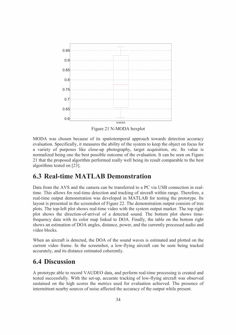
The metric was calculated per clip on all the corpus of evaluation with help of USF-DATE tool developed by South Florida University. The results are presented using a non-parametric statistical plot called boxplot in which the statistical measures median, upper and lower quartiles and minimum and maximum values are summarized [23].

0 0.5 1 1.5 2 2.5 3 3.5 40

10

20

30

40

50

60

70

80

90

100

KalmanVAUDEO Loc.

34

Figure 21 N-MODA boxplot

MODA was chosen because of its spatiotemporal approach towards detection accuracy evaluation. Specifically, it measures the ability of the system to keep the object on focus for a variety of purposes like close-up photography, target acquisition, etc. Its value is normalized being one the best possible outcome of the evaluation. It can be seen on Figure 21 that the proposed algorithm performed really well being its result comparable to the best algorithms tested on [23].

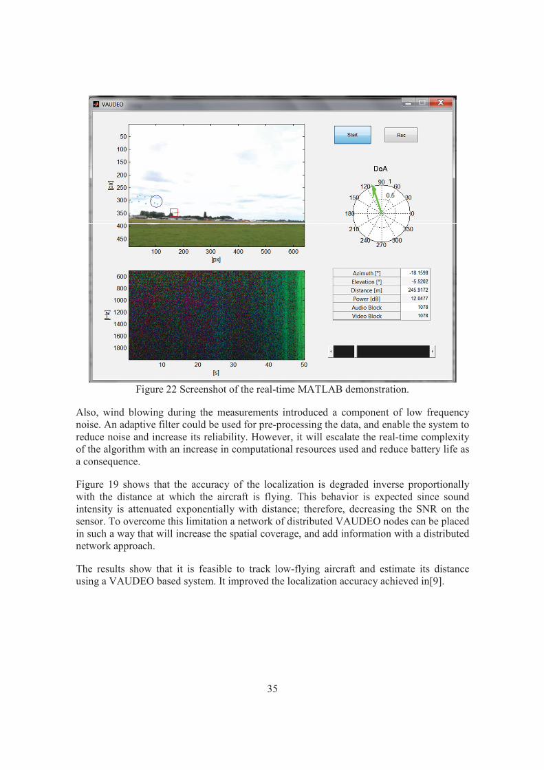
6.3 Real-time MATLAB Demonstration Data from the AVS and the camera can be transferred to a PC via USB connection in real-time. This allows for real-time detection and tracking of aircraft within range. Therefore, a real-time output demonstration was developed in MATLAB for testing the prototype. Its layout is presented in the screenshot of Figure 22. The demonstration output consists of tree plots. The top-left plot shows real-time video with the system output marker. The top right plot shows the direction-of-arrival of a detected sound. The bottom plot shows time-frequency data with its color map linked to DOA. Finally, the table on the bottom right shows an estimation of DOA angles, distance, power, and the currently processed audio and video blocks.

When an aircraft is detected, the DOA of the sound waves is estimated and plotted on the current video frame. In the screenshot, a low-flying aircraft can be seen being tracked accurately, and its distance estimated coherently.

6.4 Discussion A prototype able to record VAUDEO data, and perform real-time processing is created and tested successfully. With the set-up, accurate tracking of low-flying aircraft was observed sustained on the high scores the metrics used for evaluation achieved. The presence of intermittent nearby sources of noise affected the accuracy of the output while present.

0.6

0.65

0.7

0.75

0.8

0.85

0.9

0.95

N-MODA

35

Figure 22 Screenshot of the real-time MATLAB demonstration.

Also, wind blowing during the measurements introduced a component of low frequency noise. An adaptive filter could be used for pre-processing the data, and enable the system to reduce noise and increase its reliability. However, it will escalate the real-time complexity of the algorithm with an increase in computational resources used and reduce battery life as a consequence.

Figure 19 shows that the accuracy of the localization is degraded inverse proportionally with the distance at which the aircraft is flying. This behavior is expected since sound intensity is attenuated exponentially with distance; therefore, decreasing the SNR on the sensor. To overcome this limitation a network of distributed VAUDEO nodes can be placed in such a way that will increase the spatial coverage, and add information with a distributed network approach.

The results show that it is feasible to track low-flying aircraft and estimate its distance using a VAUDEO based system. It improved the localization accuracy achieved in[9].

36

37

7 Conclusions and Further Work

An algorithm for detecting and tracking aircraft at practical ranges using a multi-coordinate VAUDEO prototype was designed, demonstrated and validated. Up to this point, the information provided in this thesis will be useful in understanding the operating principles of the VAUDEO combination, which information can be extracted with further processing, and how to make intelligent decisions to escalate the system to a distributed network of interdependent nodes. This chapter will summarize the results achieved with the prototype; describe its limitations, possible improvements, and conclude with suggestions for further work unveiled while writing this thesis. In Appendix A, a calibration procedure designed for the VAUDEO combination is described.

7.1 Single-node VAUDEO System In section 6.2, the result of processing the measured data shown that the algorithm is capable of detecting and tracking low-flying aircraft accurately while present on the FOV of the camera. The aircraft position estimation using information from both audio and video proved to increase in confidence and accuracy when compared to estimation using only audio. It is observed that localization error increases with the distance at which the aircraft is flying. The proposed algorithm utilizes five sources of data to detect low-flying aircraft, estimate the DoA of its propeller sound, its distance and velocity. These are: three orthogonal sound particle velocity measurements, one acoustic pressure microphone and one electro-optical device. Each one of these is equally important for the attainment of the reported performance of the prototype. Furthermore, the minimum SNR needs to be over a threshold which will be defined with further testing. The results also evidenced that the performance of the system is degraded with the distance at which the aircraft is flying. This result is intuitive since sound waves are attenuated with distance on air and the SNR is reduced.

Since detection is the first step towards accurate tracking of propeller aircraft, it is important to state the practical detection range of one VAUDEO node. Based on the localization error results showed in Figure 19 and GPS measurements, it is concluded that the low-flying aircraft recorded is tracked accurately up to approximately 1000 [m] range. This implies that an aircraft flying inside the semi-sphere with 1000 [m] radius centered on the prototype will be detected; and also tracked as long as it is inside the FOV of the camera and emits sound. Using a HD dedicated camera the range is expected to increase. A set of cameras used in combination with an AVS will provide with 360° detection and tracking capability to the VAUDEO node.

During the development of this thesis it was discovered that the distance at which the aircraft is flying could be estimated combining measurements from the AVS, the camera and the speed of sound as analyzed in section 5.7. A good estimation was observed when the aircraft is flying perpendicular to the axis of the FOV of the camera.

38

In some cases it is expected that more than one airborne vehicle will be present inside the detection range of the node. Further experiments are required to test the multiple object tracking capabilities of the prototype.

Finally, the calibration procedure based on theoretical developments to combine video and audio proposed in Appendix A was validated. It approaches the VAUDEO combination in a generic way and proved to be successful in achieving the localization error reported in section 6.

7.2 Further Work 7.2.1 Distributed VAUDEO system

The results presented so far cover the output of a single VAUDEO node. In practice, it will be useful to have a distributed, scalable network of VAUDEO sensors in order to cover larger and irregular areas. The combination of two or more nodes is expected to add interesting new possibilities like improved range of detection and tracking, better localization accuracy and distributed computing capabilities. Algorithms for signal processing and distributed computing in wireless acoustic networks have been proposed by Bertrand [25] but optimized for speech signals. His results show a practical framework to achieve distributed computing and parameter estimation within a cooperative network of wireless sensors. In the VAUDEO system a cooperative network could also be applied to improve battery life, optimize the amount of data transmitted, enable the network to repair itself in case one node is disabled, focus on some nodes while “muting” other ones, increase the SNR, etc.

It is recommended that such a network is installed and investigated.

7.2.2 Aircraft range estimation While analyzing the measured data, the possibility to estimate the distance at which the aircraft is flying with the use of one AVS and a camera became apparent. Since audio travels slower than light in air, the position estimation using audio closely follows the localization with video. With air temperature measurements, the radial distance at which the aircraft is flying could be estimated using the developments in section (5) .However, only the simplest case was analyzed. That is, when the aircraft is flying perpendicular to the axis of the VAUDEO combination. Further investigation is required to analyze the general case. In [17], the author proposed a tracking approach in which a 3D object trajectory in space is related to the image plane by a homography [26]. Using this technique it is expected that complex trajectories on 3D space can simplified to the simple case discussed in section 5.

39

References

[1] T. Basten and H.-E. de Bree, “Localization and tracking of aircraft with ground based 3D sound probes,” presented at the ERF33, Kazan, Russia, 2007.

[2] P. Shankar, “Validation of VAUDEO (Video + Audio): design of detection and classifying algorithms,” Master Thesis, Technische Universität Ilmenau, Ilmenau, 2012.

[3] E. H. G. Tijs, “Study and development of an in situ acoustic absorption measurement method,” PhD, University of Twente, Enschede, The Netherlands, 2013.

[4] A. Brutti, M. Omologo, and P. Svaizer, “Comparison Between Different Sound Source Localization Techniques Based on a Real Data Collection,” in Hands-Free Speech Communication and Microphone Arrays, 2008. HSCMA 2008, 2008, pp. 69–72.

[5] H.-E. de Bree, The Microflown. www.microflown.com, 2011. [6] A. Nehorai and E. Paldi, “Acoustic vector-sensor array processing,” Signal Process.

IEEE Trans. On, vol. 42, no. 9, pp. 2481–2491, 1994. [7] H.-E. de Bree, P. Leussink, T. Korthorst, H. Jansen, T. S. Lammerink, and M.

Elwenspoek, “The -flown: a novel device for measuring acoustic flows,” Sens. Actuators Phys., vol. 54, no. 1, pp. 552–557, 1996.

[8] H.-E. de Bree, J. Wind, and S. Sadasivan, “Broad banded acoustic vector sensors for outdoor monitoring propeller driven aircraft,” in Proceedings of DAGA, 2010.

[9] H.-E. de Bree, J. Wind, and P. de Theije, “Detection, localization and tracking of aircraft using acoustic vector sensors,” in INTER-NOISE and NOISE-CON Congress and Conference Proceedings, 2011, vol. 2011, pp. 1112–1116.

[10] S.-C. S. Cheung and C. Kamath, “Robust techniques for background subtraction in urban traffic video,” in Proceedings of SPIE - The International Society for Optical Engineering, San Jose, CA, United states, 2004, vol. 5308, pp. 881 – 892.

[11] A. L. Gilbert, M. K. Giles, G. M. Flachs, R. B. Rogers, and U. Y. Hsun, “A real-time video tracking system,” Pattern Anal. Mach. Intell. IEEE Trans. On, no. 1, pp. 47–56, 1980.

[12] P. Bourqui, “Video-based automated traffic analysis,” Vis. Interface 1998 Vanc. BC Proc., 1998.

[13] D.-S. Jang and H.-I. Choi, “Active models for tracking moving objects,” Pattern Recognit., vol. 33, no. 7, pp. 1135–1146, 2000.

[14] W. Elmenreich, “Sensor fusion in time-triggered systems,” 2002. [15] R. J. Hanson and M. J. Norris, “Analysis of measurements based on the singular

value decomposition,” SIAM J. Sci. Stat. Comput., vol. 2, no. 3, pp. 363–373, 1981. [16] P. H. Schönemann, “A generalized solution of the orthogonal Procrustes problem,”

Psychometrika, vol. 31, no. 1, pp. 1–10, 1966. [17] K. Dimitropoulos, N. Grammalidis, D. Simitopoulos, N. Pavlidou, and M. Strintzis,

“Aircraft detection and tracking using intelligent cameras,” in Image Processing, 2005. ICIP 2005. IEEE International Conference on, 2005, vol. 2, pp. II–594–7.

[18] I. D. Reid, D. W. Murray, and K. J. Bradshaw, “Towards active exploration of static and dynamic scene geometry,” in Robotics and Automation, 1994. Proceedings., 1994 IEEE International Conference on, 1994, pp. 718–723 vol.1.

[19] “Logitech HD Webcam C615 Technical Specifications,” Troubleshooting. . [20] “Photography a conceptual lens model,” Photography a conceptual lens model. .

40

[21] J. L. Crassidis and J. L. Junkins, Optimal estimation of dynamic systems, vol. 24. Chapman & Hall, 2011.

[22] E. S. Page, “Continuous Inspection Schemes,” Biometrika, vol. 41, no. 1/2, pp. 100–115, 1954.

[23] R. Kasturi, D. Goldgof, P. Soundararajan, V. Manohar, J. Garofolo, R. Bowers, M. Boonstra, V. Korzhova, and J. Zhang, “Framework for Performance Evaluation of Face, Text, and Vehicle Detection and Tracking in Video: Data, Metrics, and Protocol,” Pattern Anal. Mach. Intell. IEEE Trans. On, vol. 31, no. 2, pp. 319–336, 2009.

[24] D. Doermann and D. Mihalcik, “Tools and techniques for video performance evaluation,” in Pattern Recognition, 2000. Proceedings. 15th International Conference on, 2000, vol. 4, pp. 167–170 vol.4.

[25] A. Bertrand, “Signal Processing Algorithms for Wireless Acoustic Sensor Networks,” KU Leuven, University of Leuven, Belgium, 2011.

[26] K. J. Bradshaw, I. D. Reid, and D. W. Murray, “The active recovery of 3d motion trajectories and their use in prediction,” Pattern Anal. Mach. Intell. IEEE Trans. On, vol. 19, no. 3, pp. 219–234, 1997.

41

Appendix A

A.1 Calibration Procedure The location of the sound source estimated with the AVS should be visible on the video frame if it is inside the FOV of the camera. A coordinate system transformation between points relative to the AVS and points relative to the camera is necessary. In practice, a calibration procedure is performed to obtain a transformation matrix in the least-square sense.

First, an affine transformation model is defined according to:

Where pa is a unitary vector pointing towards the DOA of the incoming acoustic wave on the AVS coordinates, b is an origin translation, A is a transformation matrix, and pc is the transformed vector pointing towards the DOA in camera coordinates. Matrix A and vector b are unknown.

Next, since the system is intended for far-field measurements, and both sensors are placed close together, the effects of b are negligible. Therefore, it can be removed from the formulation.

(Camera points) = (transformation matrix) x (measured points AVS)

[y1 y2 y3 y4…y16]= A [x1 x2 x3 x4…x16]

Yi=[xyi yyi zyi]T

xi=[xxi yxi zxi]T

Y = A . X

3x16 = 3x3.3x16

e = AX-Y

Problem:

42

The following rules are used to solve the problem:

1.2.3.4.5.6.7.

8.

9.10. Pseudoinverse-Linearly independent rows

Solution:

In order to find the min, a matrix A that satisfies is required;

Using (8),

(A.1)

43

As demonstrated on the previous development, to find the transformation matrix A, the matrices X and Y must be obtained first. Matrix Y is straight forward and is defined dividing the video frame into 16 rectangles according to Figure 23. Each point is expressed in spatial Cartesian coordinates assuming a unitary vector. The 16 centroids are chosen as calibration points since it proved to be sufficient for this application, however, more points could provide better accuracy. The procedure to estimate a matrix X is as follows:

1. Place the prototype in an anechoic room.

2. With help of the video feed, place a speaker in the centroid of each of the rectangles previously defined in the video frame one at a time.

3. Play an impulsive sound at least 10 times per point and register the average of the measured DOA values. Repeat on all rectangles.

4. Matrix X is obtained placing the 16 averaged measurements in correspondence with matrix Y already defined.

Matrix A is then obtained replacing the matrices in relation A.1 and solving for A.

Figure 23 Calibration points in the video camera frame.