Design of a small AqueousHomogeneous Reactor forproduction of 99MoImproving the reliability of the supplychain

S. Rijnsdorp

Mas

terT

hesis

DESIGN OF A SMALL AQUEOUSHOMOGENEOUS REACTOR FOR

PRODUCTION OF 99MOIMPROVING THE RELIABILITY OF THE SUPPLY CHAIN

by

S. Rijnsdorp BSc

in partial fulfillment of the requirements for the degree of

Master of Sciencein Applied Physics

at Delft University of Technology,to be defended on Tuesday September 2, 2014 at 09:30.

faculty Applied Sciencesdepartment Radiation Science and Technology

section Nuclear Energy and Radiation Applications

supervisors Dr.ir. J.L. KloostermanDr.ir. M. Rohde

thesis committee Dr.ir. J.L. Kloosterman TU Delft, Applied Sciences, RST, NERADr.ir. M. Rohde TU Delft, Applied Sciences, RST, NERADr. Eng. L.M. Portela TU Delft, Applied Sciences, ChemE, TP

ABSTRACT

Medical isotopes are used worldwide for medical imaging and treatment of patients with differentkinds of diseases, for example thyroid diseases and blood disorders. The most widely used radio-isotope for medical imaging is 99mTc, a daughter nuclide of 99Mo. Annually, around 400,000 diag-nostical treatments using 99mTc are carried out in the Netherlands.

The characteristic aspect that makes 99mTc so useful for medical imaging is also the challenge:99mTc has a half-life of approximately 6 hours. Because also the parent nuclide 99Mo has a relativelyshort half-life (66 hours), a continuous production and supply is needed. Recently, a number ofevents occurred, disrupting the supply, which led to the wish for a more reliable production methodof radioisotopes. Currently, the entire world demand is produced in 5 reactors, meaning that anunplanned outage of one or more reactors will immediately decrease the supply of 99Mo. If morereactors are used for production of 99Mo on a smaller scale, the effect of such an event is decreased.

An aqueous homogeneous reactor (AHR) is considered a suitable candidate to produce medicalisotopes on a small scale. Various aspects contribute to the suitability, such as the relatively easyextraction of 99Mo, the possibility to use low enriched uranium (LEU) fuel and the large negativevoid and temperature feedback.

In this thesis, an AHR design is optimized to meet the Dutch demand for 99Mo for the comingyears. In the process, an existing computational model is used and improved to better describephysical phenomena that come into play when operating the reactor, such as temperature-inducedfuel expansion and creation of void bubbles. An earlier proposed geometry is used and slightly al-tered.

The designed reactor is fueled by a uranyl sulfate solution containing 225 gL−1 uranium withan inflow rate of 0.4 kg s−1 and operates at a power of 13.2 kW in steady state. At this power level,the maximum fuel temperature in the core is 316.1 K, which is well below the boiling point. Whenoperating continuously, the reactor is capable of producing an amount of 99Mo that is sufficient tomeet the estimated Dutch demand, assuming daily transport from the reactor facility.

An important result of the investigation of transient behavior in case of an unanticipated event,is that safe operation is ensured for all scenarios considered. The largest problems could occur iffor some reason the fuel level in the reactor rises significantly, but this can be easily prevented byadding supplementary outflow pipes just above the desired fuel level. In all other scenarios, thepower excursions induced by an increase in reactivity are limited by the negative feedback effects.The maximum fuel temperature stays well below the boiling point in all cases considered.

iii

CONTENTS

Abstract iii

1 Introduction 1

1.1 Nuclear fission . . . . . . . . . . . . . . . . . . . . . . . . . . . . . . . . . . . . . . . . 1

1.2 Medical isotopes . . . . . . . . . . . . . . . . . . . . . . . . . . . . . . . . . . . . . . . 3

1.3 Aqueous Homogeneous Reactors - an overview . . . . . . . . . . . . . . . . . . . . . . 5

1.4 Design considerations . . . . . . . . . . . . . . . . . . . . . . . . . . . . . . . . . . . . 12

1.5 Aim of this project . . . . . . . . . . . . . . . . . . . . . . . . . . . . . . . . . . . . . . 13

2 Theory 15

2.1 Fuel solution . . . . . . . . . . . . . . . . . . . . . . . . . . . . . . . . . . . . . . . . . 15

2.2 Radiolytic gas production . . . . . . . . . . . . . . . . . . . . . . . . . . . . . . . . . . 18

2.3 Boussinesq approximation . . . . . . . . . . . . . . . . . . . . . . . . . . . . . . . . . 20

2.4 Fuel density calculation . . . . . . . . . . . . . . . . . . . . . . . . . . . . . . . . . . . 22

2.5 Geometry . . . . . . . . . . . . . . . . . . . . . . . . . . . . . . . . . . . . . . . . . . . 24

2.6 Temperature distribution and cooling . . . . . . . . . . . . . . . . . . . . . . . . . . . 25

3 Computational codes 27

3.1 SCALE XSDRNPM . . . . . . . . . . . . . . . . . . . . . . . . . . . . . . . . . . . . . . 27

3.2 HEAT . . . . . . . . . . . . . . . . . . . . . . . . . . . . . . . . . . . . . . . . . . . . . 27

3.3 Serpent . . . . . . . . . . . . . . . . . . . . . . . . . . . . . . . . . . . . . . . . . . . . 30

3.4 Coupling between Serpent and HEAT . . . . . . . . . . . . . . . . . . . . . . . . . . . 30

3.5 Point kinetics . . . . . . . . . . . . . . . . . . . . . . . . . . . . . . . . . . . . . . . . . 31

4 Steady state calculations 33

4.1 Initial design . . . . . . . . . . . . . . . . . . . . . . . . . . . . . . . . . . . . . . . . . 33

4.2 Adjusting inflow . . . . . . . . . . . . . . . . . . . . . . . . . . . . . . . . . . . . . . . 34

4.3 12 inlets . . . . . . . . . . . . . . . . . . . . . . . . . . . . . . . . . . . . . . . . . . . . 35

4.4 Improving the model. . . . . . . . . . . . . . . . . . . . . . . . . . . . . . . . . . . . . 37

4.5 Lowering the concentration . . . . . . . . . . . . . . . . . . . . . . . . . . . . . . . . . 38

4.6 Improving the code . . . . . . . . . . . . . . . . . . . . . . . . . . . . . . . . . . . . . 39

5 Reactivity analysis 43

5.1 Uranium concentration . . . . . . . . . . . . . . . . . . . . . . . . . . . . . . . . . . . 44

5.2 Xenon concentration. . . . . . . . . . . . . . . . . . . . . . . . . . . . . . . . . . . . . 44

5.3 Void fraction . . . . . . . . . . . . . . . . . . . . . . . . . . . . . . . . . . . . . . . . . 45

5.4 Temperature . . . . . . . . . . . . . . . . . . . . . . . . . . . . . . . . . . . . . . . . . 45

5.5 Reflector water level . . . . . . . . . . . . . . . . . . . . . . . . . . . . . . . . . . . . . 46

5.6 Fuel level . . . . . . . . . . . . . . . . . . . . . . . . . . . . . . . . . . . . . . . . . . . 47

5.7 Fuel concentration in part of the water . . . . . . . . . . . . . . . . . . . . . . . . . . . 48

5.8 Linearity of feedback effects . . . . . . . . . . . . . . . . . . . . . . . . . . . . . . . . . 49

v

vi CONTENTS

6 Transient calculations 516.1 Delayed neutron fraction . . . . . . . . . . . . . . . . . . . . . . . . . . . . . . . . . . 516.2 Uranium concentration . . . . . . . . . . . . . . . . . . . . . . . . . . . . . . . . . . . 526.3 Inflow rate . . . . . . . . . . . . . . . . . . . . . . . . . . . . . . . . . . . . . . . . . . 536.4 No inflow . . . . . . . . . . . . . . . . . . . . . . . . . . . . . . . . . . . . . . . . . . . 546.5 No cooling . . . . . . . . . . . . . . . . . . . . . . . . . . . . . . . . . . . . . . . . . . 556.6 Increase in ambient temperature . . . . . . . . . . . . . . . . . . . . . . . . . . . . . . 556.7 Increase in fuel level . . . . . . . . . . . . . . . . . . . . . . . . . . . . . . . . . . . . . 566.8 Blockage of outflow pipe. . . . . . . . . . . . . . . . . . . . . . . . . . . . . . . . . . . 576.9 Water leak from the water vessel . . . . . . . . . . . . . . . . . . . . . . . . . . . . . . 586.10 Fuel leak from the reactor vessel . . . . . . . . . . . . . . . . . . . . . . . . . . . . . . 596.11 Summary . . . . . . . . . . . . . . . . . . . . . . . . . . . . . . . . . . . . . . . . . . . 60

7 Conclusion and outlook 617.1 Conclusions. . . . . . . . . . . . . . . . . . . . . . . . . . . . . . . . . . . . . . . . . . 617.2 Outlook . . . . . . . . . . . . . . . . . . . . . . . . . . . . . . . . . . . . . . . . . . . . 62

Bibliography 63

List of abbreviations 67

List of symbols 69

A Discretizations 71A.1 Discretization of the Navier-Stokes equations . . . . . . . . . . . . . . . . . . . . . . . 71A.2 Discretization of the concentration equation . . . . . . . . . . . . . . . . . . . . . . . 74A.3 Discretization of the energy balance . . . . . . . . . . . . . . . . . . . . . . . . . . . . 76

B Tables 77

1INTRODUCTION

1.1. NUCLEAR FISSIONThe fission of nuclides is in itself a natural process and occurs usually in an unstable nucleus of anatom with a high mass number. In fission reactors the process of fission is induced by the absorb-tion of neutrons by the fissile nuclides which split into new nuclides while releasing neutrons whichcan be used for another fission event. A typical decay diagram of a neutron induced fission of fissileuranium, 235U, is shown in figure 1.1.

Two different types of product can be distinguished: fission products and neutrons. Both of thesecarry kinetic energy, which can be converted into electric energy.

N

235U

A

B

N

N

N

235U

Figure 1.1: The fission process schematically visualised. After the neutron interacts with 235U,the formed U235 atom splits into two smaller isotopes A and B. Meanwhile some neutrons (N, onaverage approximately 2.45 per fission [1]) are released. These neutrons can be used for variouspurposes, for example for another fission. If the number of neutrons emerging from a fission thatinitiate a new fission is equal to or larger than 1, a chain reaction can be sustained.

Neutrons

The released neutrons are of importance for any reactor, as at least one released neutron shouldinitiate a new fission to sustain the process. However, approximately 2.45 neutrons are released perfission of 235U, leaving a possibility to extract the surplus of neutrons and use them for the study ofstructures by neutron scattering (as is done with neutrons produced in the Hoger Onderwijs Reactorin Delft), the bombardment of isotopes, and other purposes. An application of irradiating isotopes

1

2 1. INTRODUCTION

Fission Product Data Measured . . . NUCLEAR DATA SHEETS H.D. Selby et al.

values 29043. Thermal Omega West Reactor results 29054. Thermal K-factors for other fission

products 29065. Uncertainty assessment 2906

B. Q-values and fission product yields 2908C. Comparison of Q-values and fission product

yields with other measurements 2910

V. Summary 2912

Acknowledgments 2913

References 2914

A. Tabulation of R-values from Los Alamos 2917

I. INTRODUCTION

Los Alamos National Laboratory (LANL) has histori-cally maintained a laboratory system (addressing chem-istry and radiochemical analysis) for the determinationof fissions in any sample from examination of the fissionproducts in the sample. The calibration of this systemis based upon a seminal set of experiments conducted inthe 1970’s, relating fissions in 235U, 238U, and 239Pu todetector response for both thermal spectrum and fissionspectrum neutron irradiations. The details of these ex-periments are provided herein, as are the details of theevaluation of data associated with the modern basis cur-rently in use at LANL. Examination of sources of uncer-tainty is provided, along with an examination of overalluncertainty in the resulting values.

Although the experiments described in this work wereperformed several decades ago, they define the LANLunderstanding of fission product data to this day. Thedata have been reported in conference proceedings andinternal reports, but they have not previously been pub-lished in widely-available literature. The related exper-iments performed by the Interlaboratory Liquid MetalFast Breeder Reactor (LMFBR) Reaction Rate (ILRR)collaboration, led by NIST, were published, though, in aseries of detailed progress reports and final summary ar-ticles [1–15]. As will be seen later, the results from LANLRadiochemistry participation in these experiments (pub-lished as part of this paper — referred to as LANL-ILRR)are consistent with the ILRR published results from theother participating laboratories. However, the ILRR con-sensus results did not report on two of the fission prod-ucts of particular interest — 99Mo and 147Nd. For thisreason, the present LANL-ILRR data are especially im-portant for an understanding of fission leading to theproduction of these fission products.

The fission product 99Mo has played the role of a ref-erence nuclide at LANL and other laboratories, whereother fission product data are determined through ratio-measurements to this nuclide. 99Mo has a favorable half-

10-6

10-5

10-4

10-3

10-2

10-1

100

101

60 70 80 90 100 110 120 130 140 150 160 170 180

FP

Y [%

]

Mass Number

(a)

U235 thU235 fU238 f

Pu239 thPu239 f

10-1

100

101

102

103

60 70 80 90 100 110 120 130 140 150 160 170 180

FP

Y R

atio

to U

235

ther

mal

Mass Number

(b) U235 f / U235 thU238 f / U235 th

Pu239 th / U235 thPu239 f / U235 th

FIG. 1: (a)Fission chain yields from ENDF/B-VI as a func-tion of mass number for 235U, 238U, and 239Pu exposed tothermal (th) and fission-spectrum (f) neutrons. The lowerpanel (b) shows the ratio of these data to the 235U ther-mal yields, illustrating that minimal variability with fissioningspecies, and energy, is seen near A = 99, LANL’s referencefission product.

life, resulting in high count rates, and its fission prod-uct yield has minimal variability with incident neutronenergy (peak fission-product) and with fissioning species(239Pu, 235U and 238U), see Fig. 1. This paper, therefore,focuses on the determination of the 99Mo fission productdata in both fission-spectrum (“fast”) and thermal neu-tron environments. Data for other fission products, 95Zr,137Cs, 140Ba, 141,143,144Ce, and 147Nd are determinedthrough use of the ratio measurements to 99Mo fissionproduct (FP) data. Collectively, these fission productsare of special interest to the nuclear science communityfor their role in determining fission burnup, for examplein fast reactor technologies. For this reason, careful de-termination of their production is of particular interest;it was a goal of the ILRR collaboration to determine therelevant fission product data to uncertainties below 2.5%(one-standard-deviation) for their use as fission burnupmonitors.

2892

Figure 1.2: The distribution of fission products of uranium and plutonium. The green dashed lineis relevant for the reactor considered in this research, as the most occuring fission is that of 235Uby thermal neutrons. 99Mo is found in the left peak, and is one of the products with the highestyields. [2]

is the creation of 99Mo from 98Mo. This process (1.1) is referred to as neutron capture.

9842Mo+1

0 n →9942 Mo (1.1)

Fission products

The fission products, usually 2 per event, have a specific probability of being produced in the pro-cess, as depicted in figure 1.2. 99Mo can be found in the left peak, corresponding to a 6.1% yield.Obviously, after irradiation a range of fission products is available, so a selection step is needed toobtain the wanted products. The rest of the fuel can be treated as radioactive waste or be repro-cessed. This waste (either the spent fuel or waste from the reprocessing process) is usually stored inspecial facilities.

Energy

The most well-known purpose of a nuclear reactor is probably the production of electrical energy. Inevery fission event, about 200 MeV [3] becomes available. This energy comes from the difference inbinding energy between the uranium, and the fission products. In figure 1.3, the binding energy, theenergy needed to divide the nucleus into individual protons and neutrons, per nucleon, is shown.The difference between the initial and final binding energy is approximately 200 MeV, in the formof kinetic energy of the fission products and neutrons, and radiation. By collisions, kinetic energyis converted to heat, which is converted into electrical energy in nuclear power plants. One of thebenefits of using nuclear energy instead of conventional energy from coal, is the amount of fuelneeded to produce the same amount of energy. A single gram of fully fissioned uranium correspondsto the burning of roughly 3000 kg of coal in terms of the production of energy.

1.2. MEDICAL ISOTOPES 3

Figure 1.3: The binding energy per nucleon for common isotopes, 235U is found at the right side ofthe graph. The products created by fission have a higher average binding energy per nucleon; thedifference between the total binding energy before and after fission is the amount of energy thatis released in fission.

1.2. MEDICAL ISOTOPES

The term medical isotope refers to an atom that can be used for diagnostics or medical treatments.A range of radioisotopes with different characteristics and half-life times is utilized for differentpurposes, but the most common isotope (used for medical diagnostics 30 million times a yearworldwide) [4, 5] is 99mTc, in words Technetium-99 metastable. A metastable nucleus contains oneor more nucleons in excited state. This particular radioisotope has a half-life of approximately 6hours [3]. This relatively short lifetime implies that production of a large stock is useless, as afterevery day only 6.25% of the stock is left. As a consequence, continuous production and distributionof 99mTc is a prerequisite to be able to treat patients when necessary.

$9 5,/

) ! 9 & : & ! (2 $- 9

& ? / & 78 9 & & < ,$ R (? $%P 2 $- 9 !& & 4 . (?

$%-

' (1, " ).

" + !,

" 5 ! 2 Figure 1.4: A schematic diagram of the process of the decay of the unstable isotope 99Mo. All 99Modecays to 99Tc, but the majority decays to the metastable isotope, 99m Tc. The metastable productdecays in its turn to 99Tc, with a half-life of approximately 6 hours. 99Tc itself is also not a stableisotope, but the half-life is several thousands of years [6].

4 1. INTRODUCTION

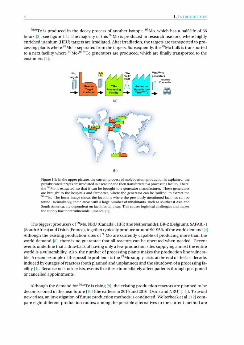
99mTc is produced in the decay process of another isotope, 99Mo, which has a half-life of 66hours [3], see figure 1.4. The majority of this 99Mo is produced in research reactors, where highlyenriched uranium (HEU) targets are irradiated. After irradiation, the targets are transported to pro-cessing plants where 99Mo is separated from the targets. Subsequently, the 99Mo bulk is transportedto a next facility where 99Mo-99mTc generators are produced, which are finally transported to thecustomers [4].

99MoProcessingFacility

GeneratorManufacture99Mo/99mTc

ReactorTarget

Irradiation

235Utargets

99Mo/99mTcgenerators

HospitalsPharmacies

99Mo“bulk”liquid

(a)

(b)

Figure 1.5: In the upper picture, the current process of molybdenum production is explained: theprefabricated targets are irradiated in a reactor and then transferred to a processing facility. There,the 99Mo is extracted, so that it can be brought to a generator manufacturer. These generatorsare brought to the hospitals and farmacies, where the generator can be ‘milked’ to extract the99m Tc. The lower image shows the locations where the previously mentioned facilities can befound. Remarkably, some areas with a large number of inhabitants, such as southeast Asia andSouth America, are dependent on facilities far away. This causes logistical challenges and makesthe supply line more vulnerable. (Images: [7])

The biggest producers of 99Mo, NRU (Canada), HFR (the Netherlands), BR-2 (Belgium), SAFARI-1(South Africa) and Osiris (France), together typically produce around 90-95% of the world demand [4].Although the existing production sites of 99Mo are currently capable of producing more than theworld demand [8], there is no guarantee that all reactors can be operated when needed. Recentevents underline that a drawback of having only a few production sites supplying almost the entireworld is a vulnerability. Also, the number of processing plants makes the production line vulnera-ble. A recent example of the possible problems is the 99Mo supply crisis at the end of the last decade,induced by outages of reactors (both planned and unplanned) and the shutdown of a processing fa-cility [4]. Because no stock exists, events like these immediately affect patients through postponedor cancelled appointments.

Although the demand for 99mTc is rising [9], the existing production reactors are planned to bedecomissioned in the near future [10] (the earliest in 2015 and 2016 (Osiris and NRU) [11]). To avoidnew crises, an investigation of future production methods is conducted. Wolterbeek et al. [12] com-pare eight different production routes; among the possible alternatives to the current method are

1.3. AQUEOUS HOMOGENEOUS REACTORS - AN OVERVIEW 5

photonuclear reaction of 100Mo, direct production of 99mTc by irradiation of 100Mo with protons, gelgenerator technology and aqueous homogeneous reactors [4, 13].

In the light of the Non-Proliferation Treaty [14], which embodies a goal of achieving nucleardisarmament, the aqueous homogeneous reactor is an ideal substituent for current reactors con-sidering its possibility to use low enriched uranium as fuel. Also it is capable of producing 99Mousing only 1% of the uranium currently needed for a similar production in nuclear reactors [15].

In the Organisation for Economic Co-operation and Development (OECD) report on the pathto a reliable supply chain a list of criteria for production methods is posed [11]. Just looking at thenon-legal and non-economical criteria an assessment of the suitability of the AHR can be made:

• Technology maturityAHRs have been built and operated for over 50 years in different forms, with different fuels.

• Production capacityOne small AHR (core volume of 40 liters) is capable of producing a sufficient amount of 99Moto satisfy the Dutch demand.

• ProcessingExtraction of the 99Mo is achieved by an absorption process, with high yield (90%).

• LogisticsFiltering and extraction can be done at the production site, eliminating a transport step.

• WasteCompared to traditional methods, only 1% of the waste is produced for a similar amount of99Mo.

• Proliferation resistanceThe AHR can be fueled with LEU, conform the Non-Proliferation Treaty.

• Other isotope production potentialDuring irradiation, a wide range of products is created, so with adequate filtering it should bepossible to extract other isotopes.

From this assessment, the conclusion can be drawn that the AHR is an important alternative for thefuture production of medical isotopes.

1.3. AQUEOUS HOMOGENEOUS REACTORS - AN OVERVIEW

LOPO - 1944The homogeneous reactor was one of the first reactors built after the first nuclear reactor, the ChicagoPile-1, went critical. The first reactor of this type was constructed at the end of 1943, running on auranyl sulfate solution containing uranium enriched to 14%, being referred to as the "water-boiler"for security reasons. This name might be misleading because it suggests that the solution boils,however the bubbles observed in the reactor were hydrogen and oxygen bubbles which arose fromthe radiolysis of the solvent, water. In 1944, the LOPO (for Low Power) went critical using a uranylsulfate solution of 565 gram 235U dissolved in 13 liters of light water contained in a sphere of 30cm diameter. The abscence of an adequate cooling system and a shield limited the power to 50mW. [16, 17]

6 1. INTRODUCTION

Boiler wCom

from Hmodific

TidgTspTrpsAnthddinincteCrethfo

SUPOdeactivafor man

Cd safety curtain

Overflow chamber

Level electrodes

Cd control rod

Fuel vessel

Fuel solution

BeO reflector

Graphite reflector

Level electrode

Air pipe

Dump basin

Figure 1.6: A schematic cross section of the Low Power AHR. The spherical reactor, filled with anuranyl sulfate solution, is surrounded by graphite and beryllium oxide reflectors. The fuel can bereleased from the core using the valve at the bottom of the dump bassin. A cadmium control rodis used to maintain criticality. [16]

HYPO - 1944After dismantling the LOPO, a reactor called HYPO (for High Power) was constructed, which couldbe operated at a power level of several kW. With this reactor, cross section studies were performed,while the precursor was only used as a concept study and for determination of the critical mass.The fuel for the HYPO was contained in a similar stainless steel spherical shell with walls twice asthick as the LOPO, approximately 1.6 mm. The reflector was changed partly to a graphite thermalcolumn, and cooling coils were added to be able to run the reactor at higher power. Moreover, thefuel was changed to an uranyl nitrate solution, containing 808 grams of 235U in 13.65 L solution.Considering the intended experiments, a ‘glory hole’ was constructed, giving staff the possibility toplace samples in the high flux areas of the reactor. [17] The total construction costs for this reactorare estimated at $500,000. [16, 18]

SUPO - 1951As the neutron flux requirements for experiments rose, the HYPO was modified in 1950 to perform ata higher power level with a higher neutron flux (35 kW and 1012cm−2s−1 respectively). The modifica-tions included an improved cooling installation enhancing the removal of heat, a higher enrichment(88.7%), a replacement of the beryllium oxide parts of the reflector by graphite and the incorpora-tion of a system to recombine H2 and O2 gasses to reduce the risk at explosions. Eventually, SUPO(short for Super Power) was taken out of operation in 1974. Along with material experiments, alsothe transient behavior of the reactor was investigated. Reactivity increases led to an increase in gasproduction, resulting in a lower density in the fuel solution, reducing the moderating ability andtherefore leading to a decrease in reactivity. This negative void reactivity coefficient is an importantinherent safety aspect of the AHR. [16]

1.3. AQUEOUS HOMOGENEOUS REACTORS - AN OVERVIEW 7

(a) 1 | P a g e

Design Principals for Aqueous Homogeneous Reactors

LA-UR 11-06788

John R. Ireland

Civilian Nuclear Programs (SPO-CNP)

Los Alamos National Laboratory, J590, P.O. 1663, Los Alamos, NM 87545

ABSTRACT

Los Alamos National Laboratory developed and operated reactors using fissile solution fuels for

over 65 years. The primary purpose of these reactors was to provide a reliable and predictable

neutron flux for experimental nuclear physics, detector, and alarm evaluation; however,

surprisingly little detail exists on reactor operating characteristics, particularly at steady-state.

What data is available has been catalogued and extended by theoretical treatment to develop a

prescription for successful design for aqueous homogeneous reactors (AHR) to produce 99

Mo.

Approaches to management of radiolytic gas, temperature effects, and impact on stability are

discussed. In addition results of recent experiments on a variety of fuel types are presented.

INTRODUCTION

At the dawn of the nuclear age over six decades ago little experimental data was available to test

the theoretical concepts emerging in nuclear physics. At Los Alamos National Laboratory it was

realized that a reactor fueled with uranium in solution could be rapidly produced and would

likely provide a sufficient neutron flux to address the major questions related to cross section and

critical mass. Hence, the third reactor ever built was a uranyl sulfate fueled reactor, dubbed

LOPO, for Low Power. LOPO was placed into operation at Los Alamos in 1944 with Enrico

Fermi at the controls.

Soon thereafter a second reactor, HYPO (High Power), was constructed, followed by a third,

SUPO (Super Power). Both were fueled with uranyl nitrate, since it was realized that uranium

metal was easier to dissolve in nitric acid. SUPO operated at LANL from 1951 until 1974,

amassing over 600,000 kWhr of operation. A picture and cross section diagram of SUPO is

shown in Figure 1.

(b)

Figure 1.7: In the schematic cross section the large amount of cooling water containing coils canbe seen. The image on the right is an actual picture taken from the SUPO reactor. The tube that isplaced in the middle of the reactor is the previously mentioned ‘glory hole’. [19]

HRE - 1952From 1952 to 1954, the Homogeneous Reactor Experiment - 1 (HRE-1) reactor was operated. Inthese 2 years, the nuclear stability of a fuel-circulating reactor was demonstrated, at power levelsof several hundreds of kilowatts. The fuel, a 93% enriched uranyl sulfate solution, was circulatedthrough the core at a rate of approximately 40 L min−1. The core was a vessel of 45 cm diameterput in a pressure vessel, and the reactor used heavy water as a reflector. Steam produced in a heatexchanger powered a turbine, leading to an electrical power output of 140 kW. During experimentsthe discovery that a copper catalyst helps to recombine produced oxygen and hydrogen to water wasmade. The successor of the HRE-1, called HRE-2 or Homogeneous Reactor Test (HRT), had as maingoal to prove the ability to run a homogeneous reactor continuously (an important characteristicfor the reactor designs considered in this thesis), along with other goals such as testing methods forremoval of fission and corrosion products. Uranyl sulfate was still used as fuel, but this time heavywater rather than light water was used as a solvent. During steady state operation, power excur-sions occurred, temporarily raising or lowering the reactor power. Investigation of these excursionsshowed that they were initiated by movement of uranium through the core. [17, 20]

8 1. INTRODUCTION

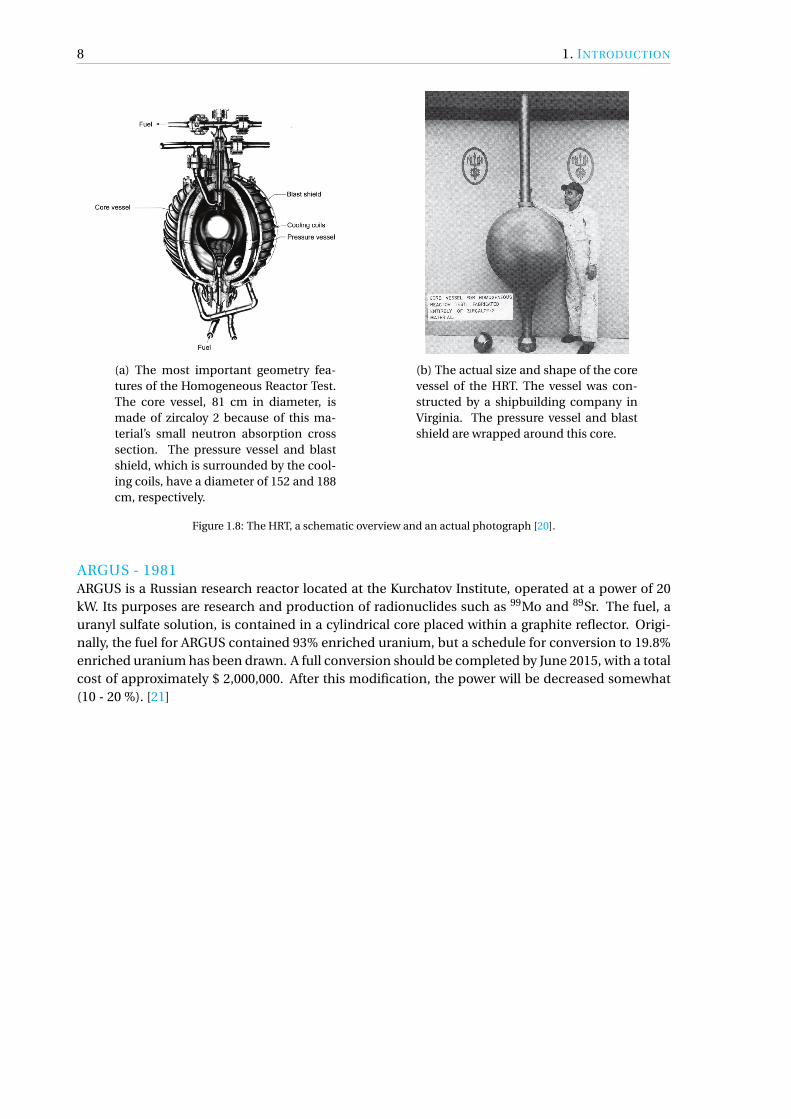
(a) The most important geometry fea-tures of the Homogeneous Reactor Test.The core vessel, 81 cm in diameter, ismade of zircaloy 2 because of this ma-terial’s small neutron absorption crosssection. The pressure vessel and blastshield, which is surrounded by the cool-ing coils, have a diameter of 152 and 188cm, respectively.

Fig. 16. Core vessel for the HRT. The vessel was fabricated by

Newport News Shipbuilding and Drydock Company of Newport

News, Virginia. (ORNL Photo 24103)

which they could be drained at intervals for D2O recovery, sampling, and removal for further

processing and disposal. The hydroclones did remove some solid fission products and a larger amount

of corrosion products, but material balances and radiation scans of components showed that most

were deposited in the heat exchanger and other components.

Provisions for maintenance were given careful attention in the design. The reactor was

surrounded by a 2 ft thick neutron-absorbing shield to reduce activation of equipment. All of the

primary system was below grade in a cell with a steel lining that could be flooded to lower the

radiation level during maintenance. The top shield, as seen in Fig. 17, was made in sections that could

be removed and replaced with a work shield when maintenance was to be done. The equipment was

made accessible from above with provisions for ease of removal, such as all bolts pointing up and the

number of separate parts minimized. And tools and procedures were tested on mock-ups before being

used in the reactor cell. (The cell wall was heavy enough to contain the contents of the entire primary

system if it were unintentionally released at full operating pressure.)

Preoperational testing was interrupted by the discovery of chloride-ion-induced stress corrosion

cracking that required replacement of 132 high-pressure flanges. The chloride was found to have

resulted from the fabricator’s incomplete removal of a chloride-containing drawing compound from

long stainless-steel tubes that were attached to flanges for leak detection.

20

(b) The actual size and shape of the corevessel of the HRT. The vessel was con-structed by a shipbuilding company inVirginia. The pressure vessel and blastshield are wrapped around this core.

Figure 1.8: The HRT, a schematic overview and an actual photograph [20].

ARGUS - 1981ARGUS is a Russian research reactor located at the Kurchatov Institute, operated at a power of 20kW. Its purposes are research and production of radionuclides such as 99Mo and 89Sr. The fuel, auranyl sulfate solution, is contained in a cylindrical core placed within a graphite reflector. Origi-nally, the fuel for ARGUS contained 93% enriched uranium, but a schedule for conversion to 19.8%enriched uranium has been drawn. A full conversion should be completed by June 2015, with a totalcost of approximately $ 2,000,000. After this modification, the power will be decreased somewhat(10 - 20 %). [21]

1.3. AQUEOUS HOMOGENEOUS REACTORS - AN OVERVIEW 9

After conversion, the reactor “ARGUS” purpose will remain the same: to search for the best

physical-technical solutions when developing nuclear-physical methods of analysis and

control as well as to develop work on production of radionuclides. When the reactor

“ARGUS” is converted to low-enriched fuel, one of the main phases of development of the

high technology of production of fission radionuclides molybdenum-99, strontium-89 etc

will be finished.

2. “Argus” Reactor

Argus is a 20kW homogeneous solution thermal-neutron reactor. The reactor core is the

uranyl sulfate water solution enriched up to 90 % in 235

U located in a welded cylindrical

vessel with a hemispherical bottom and a flat cover. Vertical "dry" channels are installed in

the vessel: the central and two symmetric peripheral ones. Control and regulation rods are

located in the peripheral channels. The core elements contacting with a fuel solution are

made from stainless steel. The reactor vessel is surrounded with a side and bottom graphite

reflectors (Fig. 1). There are five vertical channels and one horizontal channel for neutron

beam extraction in the reflector.

Figure 1 – Scheme of the Reactor Argus

2 - !2 Recombiner

Reactor Vessel with UO2SO4

Heat Exchanger

Condensate Collector

Reflector

(Graphite)

Recombiner Holder

Figure 1.9: An overview of the ARGUS reactor, displaying the core and attached circuits. An emi-nent feature is the geometry of the core. Whereas previously mentioned reactors all had a sphericalcore, the ARGUS reactor has a cilindrical one with a hemisphere attached at the bottom. Radiolyticgas produced in the reactor flows through the H2-O2 recombiner, condensates and then returnsto the fuel solution as water. [21]

SILENE - 1974SILENE was originally designed to investigate accidents originating from situations in which sud-denly a critical mass is reached. The core consists of a cyclindrical tank containing the fuel solution,with a small annular cylinder for the control rod in the center. The fuel solution is a 71 gram perliter uranyl nitrate solution, with an enrichment of 93%. Traditionally, the reactor was used to studycriticality accidents, simulated by retracting the control rod. Three operation modes are the pulsemode, the free evolution mode and the steady state mode. In pulse mode, the control rod is retractedquickly, leading to a short power excursion to a very high level. In free evolution mode, the controlrod is removed more carefully, while in steady state mode the reactor operates for a longer time at acertain power level. [22]

10 1. INTRODUCTION

1

2

3

4

56

7

8

Figure 1.10: The layout of the reactor part of the SILENE facility. The rod drive mechanisms (1) atthe top are used to move the control rod (2) up and down the central axial channel (3). The heightand temperature of the fissile solution (4) are tracked by the level measurement devices (5) andthermocouples (6), to pass information on the state of the reactor. (7) is a pressure transducer, and(8) is a test capsule in which samples can be put in the center of the reactor to be irradiated. [23]

Figure 1.11: An overview of the SILENE reactor. The processing facilities are found one floor belowthe reactor itself. Fission products and fission gases are extracted, and the solution is reprocessedto be reinserted. The actual reactor, displayed on the upper floor in this figure, is shown in moredetail in figure 1.10. [23]

1.3. AQUEOUS HOMOGENEOUS REACTORS - AN OVERVIEW 11

MIPR BY NPICThe Medical Isotopes Production Reactor concept as designed by the Nuclear Power Institute ofChina uses 100 L of a 90% enriched uranyl nitrate fuel solution in a cylindrical vessel (70 cm diameterand 73 cm height) and operates at 200 kW in steady state, while the power is controlled by a controlrod. On average, the fuel temperature is around 343 K; well below the boiling point. Running for 100cycles a year consisting of a 24 hour running period and a 48 hour shutdown, the annual productionis 100,000 curies of 99Mo, which corresponds to 220 6-day curie per cycle. The reactor fuel can beeither a uranyl sulfate or uranyl nitrate solution, and both LEU and HEU can be used. In practice, auranyl nitrate solution is chosen to ease the extraction process. [24, 25]

SAMOPThe Subcritical Assembly for Molybdenum Production, abbreviated SAMOP, consists of a 25.7 litercore tank surrounded by graphite reflectors, filled with 22.7 liters of uranyl nitrate solution. Thisentire system is placed in a tank filled with water for cooling purposes. The critical uranium con-centration depends on factors as the thickness of the reflector and the placement of the reactor inthe cooling tank, but has a minimum value of 300 gram 20% enriched uranium per liter. After ir-radiation, the fuel is first stored for some time in the delay tank, subsequently the molybdenum isextracted in the extraction column. In the reconditioning facility, the remainder of the solution isreconditioned and prepared to be reinserted in the reactor. [26]

Extraction

column

Reconditioning Facility

Dump tank

Delay tank

UN solution tank Cooling water

Core tank

Graphite reflector

Figure 1.12: In the schematic above, the entire production process of 99Mo is displayed. The uranylnitrate solution flows from the storage tank to the reactor. After irradiation the fuel ‘cools down’ inthe delay tank, before the 99Mo is extracted [26].

SHEBASHEBA, Solution High-Energy Burst Assembly, is a homogeneous reactor located at Los Alamos Na-tional Laboratory, New Mexico. The core consists of a cylinder (diameter 49 cm, fuel height 43-45cm) with a boron carbide control rod in the center, surrounded by the fuel, either a uranyl fluoridesolution of 5% enrichment or a uranyl nitrate solution of 20% enrichment. A short list of goals ofthe SHEBA project is provided by Capiello, topped by ‘study the behavior of nuclear excursions ina low-enrichment solution’. To achieve this goal, SHEBA is often operated in a free run to simu-

12 1. INTRODUCTION

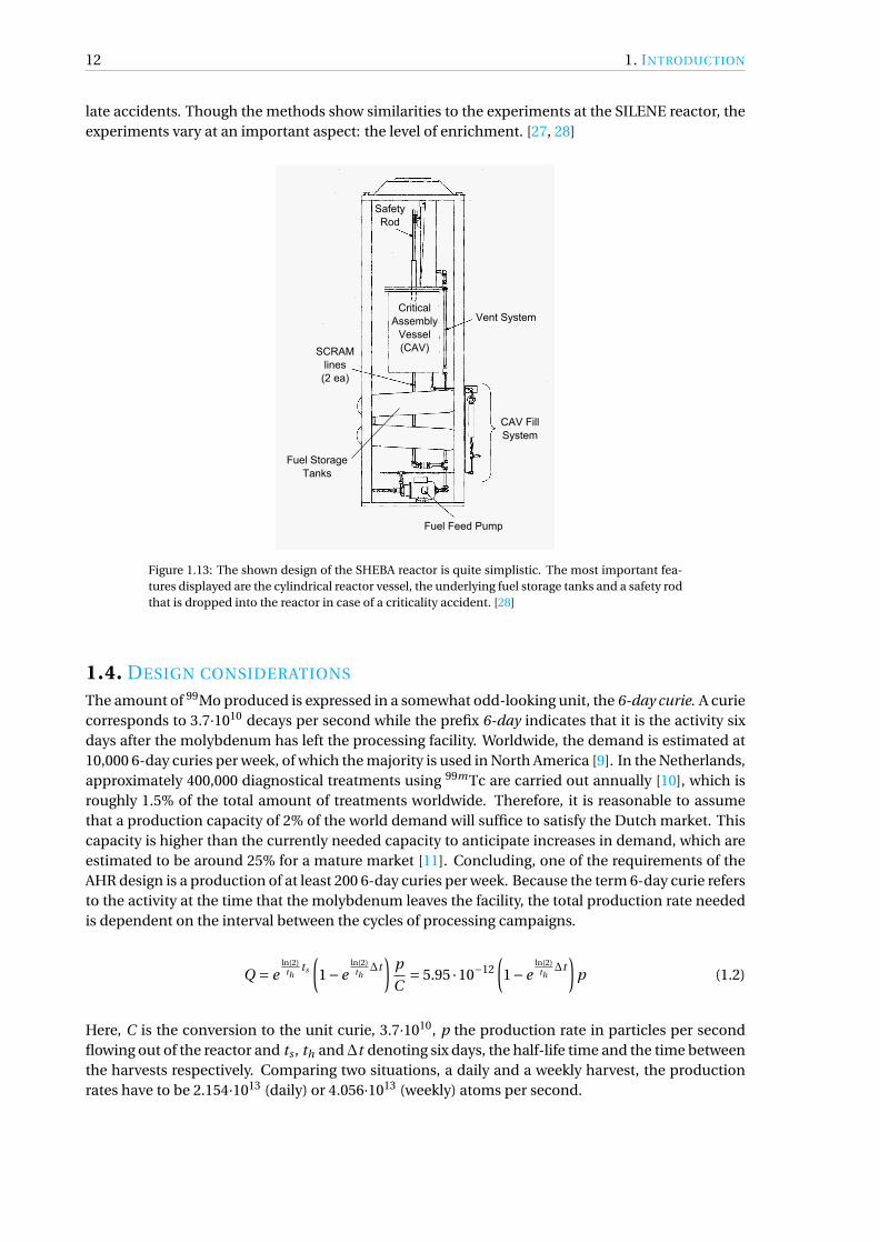
late accidents. Though the methods show similarities to the experiments at the SILENE reactor, theexperiments vary at an important aspect: the level of enrichment. [27, 28]

SCRAMlines

(2 ea)

CriticalAssembly

Vessel(CAV)

Fuel Feed Pump

CAV FillSystem

Vent System

SafetyRod

Fuel Storage Tanks

Figure 1.13: The shown design of the SHEBA reactor is quite simplistic. The most important fea-tures displayed are the cylindrical reactor vessel, the underlying fuel storage tanks and a safety rodthat is dropped into the reactor in case of a criticality accident. [28]

1.4. DESIGN CONSIDERATIONS

The amount of 99Mo produced is expressed in a somewhat odd-looking unit, the 6-day curie. A curiecorresponds to 3.7·1010 decays per second while the prefix 6-day indicates that it is the activity sixdays after the molybdenum has left the processing facility. Worldwide, the demand is estimated at10,000 6-day curies per week, of which the majority is used in North America [9]. In the Netherlands,approximately 400,000 diagnostical treatments using 99mTc are carried out annually [10], which isroughly 1.5% of the total amount of treatments worldwide. Therefore, it is reasonable to assumethat a production capacity of 2% of the world demand will suffice to satisfy the Dutch market. Thiscapacity is higher than the currently needed capacity to anticipate increases in demand, which areestimated to be around 25% for a mature market [11]. Concluding, one of the requirements of theAHR design is a production of at least 200 6-day curies per week. Because the term 6-day curie refersto the activity at the time that the molybdenum leaves the facility, the total production rate neededis dependent on the interval between the cycles of processing campaigns.

Q = eln(2)

thts

(1−e

ln(2)th∆t

)p

C= 5.95 ·10−12

(1−e

ln(2)th∆t

)p (1.2)

Here, C is the conversion to the unit curie, 3.7·1010, p the production rate in particles per secondflowing out of the reactor and ts , th and∆t denoting six days, the half-life time and the time betweenthe harvests respectively. Comparing two situations, a daily and a weekly harvest, the productionrates have to be 2.154·1013 (daily) or 4.056·1013 (weekly) atoms per second.

1.5. AIM OF THIS PROJECT 13

1.5. AIM OF THIS PROJECT

As discussed before, the vulnerability of the current supply chain of 99Mo is the limited amount ofproduction and processing facilities. If an AHR is used to produce 99Mo at a smaller scale than inthe current production facilities, the reliability of the supply chain will be improved because of tworeasons. First, the number of production facilities is increased, which means that an outage of onereactor has a smaller effect on the total production. Second, the irradiated fuel can be processedat the production site, eliminating the need for separate processing facilities and simplifying theproduction process as a result. Therefore, an AHR which can produce approximately 2% of theglobal demand is designed. The design proposed by Huisman [29] is optimized, while additions tothe computational model are made to approximate reality more closely. A leading goal is:

To design an aqueous homogeneous reactor which can produce approximately 2 percent ofthe global demand of 99Mo.

2THEORY

2.1. FUEL SOLUTIONThe fuel of an aqueous homogeneous reactor is an uranyl salt dissolved in water. Looking at earlierreactors, the choice of salt is narrowed down to uranyl nitrate (UO2(NO3)2), uranyl sulfate (UO2SO4)and uranyl fluoride (UO2F2), which have all proven to be appropriate candidates. A comparison be-tween the characteristics of the salts has to be made to determine the most ideal fuel. In general,lowering the pH of the solution will increase the solubility of the uranyl salts. [17]

Uranyl nitrate

Uranyl nitrate was used as a fuel in the HYPO and SUPO reactors [16] and is the primary choice forthe SAMOP reactor [30]. 99Mo is more easily extracted from an uranyl nitrate solution than fromuranyl sulfate because the distribution coefficient Kd , the ratio of 99Mo absorbed to the concen-tration 99Mo in the solvent, is higher for a uranyl nitrate solution. This is because competition foradsorption sites between molybdenum and sulfate is stronger than between molybdenum and ni-trate [15, 31]. Regarding the production of radiolytic gas, a uranyl nitrate solution brings additionaldifficulties, since besides H2 and O2, nitrogen oxide (NOx ) gases are formed [32]. Furthermore, alarge increase of the pH is observed after irradiation. A pH too high can lead to precipitation of so-lutes present because of the decreased solubility [31].

Uranyl sulfate

Uranyl sulfate was used as fuel in the first AHR that reached criticality, the LOPO [16], and also inthe HRE-1 and HRE-2 reactors. Less neutron absorption and a higher solubility were used as argu-ments in favor of using uranyl sulfate [17]. Although uranyl sulfate has a lower distribution coeffi-cient than uranyl nitrate, implicating a less efficient separation of the produced molybdenum fromthe irradiated fuel, it is possible to extract 99Mo from a uranyl sulfate solution with a purity of over90% [31, 33].

Uranyl fluoride

Traditionally, uranyl fluoride is not often used in AHRs, but SHEBA was designed to have the possi-bility to run on UO2F2 [27]. Taking only neutron capture into account, uranyl fluoride is an excellentoption because the capture cross section of fluorine is low compared to that of sulfate and nitrate.However, during irradiation hydrogen fluoride (HF) is produced, present in both liquid and vapor

15

16 2. THEORY

phase, which is highly corrosive towards zirconium and titanium and to a lesser extent towardsstainless steel [17]. Research has indicated that the use of uranyl fluoride indeed leads to corrosionof the stainless steel cladding [28].

The absorbtion cross sections of sulfur, fluorine and nitrogen for thermal neutrons are listed intable 2.1 [34], while table 2.2 summarizes the advantages and drawbacks of the treated salts.

Table 2.1: Relevant microscopic absorbtion cross sections (for thermal neutrons) of the con-stituent atoms of the salts. For the atoms N, F, S and O, the cross section is given for a mixtureof isotopes.

Isotope Cross section (barn)

N 1.9

F 0.0096

S 0.53

O 0.00019234U 100.1235U 680.9238U 2.68

Table 2.2: The benefits and drawbacks of the different salts.

UO2(NO3)2 + Easier 99Mo extraction compared to uranyl sulfate+ Extensive knowledge through use in earlier reactors– Production of additional gaseous products (NOx )– pH fluctuations, possible precipitation

UO2SO4 + Extensive knowledge through use in earlier reactors+ pH stable upon radiation– Efficiency of 99Mo extraction slightly lower compared to uranyl nitrate

UO2F2 + Low neutron capture cross section– Production of HF, which causes corrosion

THE INFINITE MULTIPLICATION FACTOR k∞To gain more insight into the neutronic properties of the aforementioned salts the multiplicationvalue can be investigated. This is done for the three salts, treated as an infinite homogeneous mate-rial. The parameter that is changed during the comparison is the uranium concentration, which isset equal for all salts. This implies that, because of differences in molecular weight and density, thevolumetric percentage occupied by water is different for each salt. In figure 2.1, the infinite multi-plication factor is shown for different salts and different concentrations of uranium.

2.1. FUEL SOLUTION 17

0 50 100 150 200 250 300 350 400 450 500 5500.9

1

1.1

1.2

1.3

1.4

1.5

1.6

1.7

Uranium concentration [g L−1

]

k∞

[−

]

UO2SO

4

UO2(NO

3)2

UO2F

2

Figure 2.1: The value of k∞ versus the concentration of the different salts, expressed in grams ofuranium per liter, for an enrichment of 20%. The differences between the curves are caused bydistinct cross sections, molecular weights and densities. These last two also affect the volumefraction of water.

EXTRACTION

Regarding the fact that the 99Mo is dissolved in the fuel solution after irradiaton, a method is neededto extract the 99Mo from that solution. Proposed techniques rely on chemical sorbtion processes inwhich two aspects are important: the capture yield (the fraction of the 99Mo in the fuel solution thatis captured by the sorbtion material) and the stripping yield (the fraction of the 99Mo that can berecovered from the sorbtion material). Alumina was traditionally used as sorbent for molybdenumrecovery, but currently some specifically designed sorbent materials are available for this purpose.

In 1999, Ponomarev-Stepnoy et al. claimed the invention of an AHR using a uranyl sulfatefuel [33], as shown in figure 2.2, and a solid polymer sorbent to absorb the produced 99Mo [35].Using this sorbent, 99% of the 99Mo in the fuel solution (with a pH of 1) can be absorbed, withoutabsorbing any 235U. However, whether they use a HEU or LEU fuel is not mentioned in the patents.

Vandegrift et al. [36] investigated four sorbents (alumina, Radsorb, Isosorb and PZC) to deter-mine their efficiency in absorbing 99Mo from uranyl nitrate and uranyl sulfate solutions. Radsorb,

Reactor3vessel

Free3volume

Uranyl3sulfate3solution

Pump

Heat3exchanger

Sorbent

Eluting3solution

Transfer3container

1

2

3 4

Figure 2.2: The most essential parts of the facility proposed by Ponomarev-Stepnoy et al. Thefuel is pumped from the reactor vessel, through the heat exchanger to the column containing thesorbent. When the column is filled, valve 1 is closed. Subsequently, valve 4 is opened and the fuel(without the extracted 99Mo) is returned to the reactor vessel. When no fuel is left in the sorbtioncolumn, valve 4 is closed and valves 2 and 3 are opened. The molybdenum in the sorbtion columnis solved in the eluting solution (a 10M nitric acid solution) and stored [33].

18 2. THEORY

Isosorb [37] and PZC (polyzirconium compound) are solid sorbents, specifically designed for extrac-tion of 99Mo. The most important conclusions drawn from this experimental comparison are that asorbent column can be used to efficiently extract 99Mo from LEU uranyl sulfate and uranyl nitratefuel solutions. Furthermore, it becomes clear that the specifically designed sorbents perform betterthan the alumina, and that separation of 99Mo can be done more efficiently from uranyl nitrate so-lutions than from uranyl sulfate solutions.

A titanium based sorbent, TiO2, has been introduced by Ling et al. [38] as an alternative for thetraditional alumina sorbent used in the process of capture chromatography. It has a higher selectiv-ity and capacity than alumina for 99Mo in concentrated uranyl sulfate solutions. Both the captureand the stripping yield are approximately 95%.

Although the extraction of 99Mo from an uranyl nitrate solution can be achieved more easilythan from an uranyl sulfate solution, recent experiments have shown that 99Mo can be extractedfrom uranyl sulfate fuel solutions with an efficiency larger than 90 % as discussed above. Therefore,from an extraction point of view, there is no preference for uranyl sulfate or uranyl nitrate as fuel.

Based on the aformentioned information, uranyl sulfate is chosen as fuel for the AHR. Theuranyl fluoride solution is not considered as an appropriate option due to the possible corrosion,which can cause leaks. Also, there is less knowledge available on the subject of fission product sepa-ration. Uranyl sulfate is chosen because the disadvantages of using uranyl nitrate (possible precip-itation and formation of NOx gases) are considered larger than the disadvantage of uranyl sulfate(suboptimal extraction of 99Mo).

PH ADJUSTMENT

As stated earlier, lowering the pH of the solution increases the solubility and therefore preventsprecipitation. To lower the pH, an amount of acid is added, sufficient to reduce the acidity of thesolution to a pH of 1. An ideal acid will split fully, so that a minimal amount of acid has to be added.The polyprotic sulfuric acid (H2SO4) seems a reasonable choice, as it fulfills this requirement whileno difficulties as increased corrosion rates occur. Upon solving the acid one H+ ion is split off:

H2SO4 → H++HSO−4 (2.1)

The HSO−4 splits partly, i.e., it engages itself in an equilibrium with H+ and SO2−

4

HSO−4 ↔ H++SO2−

4 (2.2)

with an equilibrium constant Kz of 0.01

Kz =[H+][

SO2−4

][HSO4

−](2.3)

Solving equation (2.3) using the imposed constraint that the pH of the fuel solution should be equalto 1

(pH =−log

[H+])

, approximately 9.7·10−2 mole of sulfuric acid is needed in a liter of fuel solu-tion.

2.2. RADIOLYTIC GAS PRODUCTIONA characteristic inherent to the AHR is the generation of gas in the fuel solution, due to the radiolysisof water. The slowing down of the fission fragments and neutrons in the liquid results in dissociationof water into H2 and O2, amongst others (such as hydrogen peroxide, H2O2) [39]. These products

2.2. RADIOLYTIC GAS PRODUCTION 19

can react with each other to form water again, however, for fission recoil particles this reaction isrelatively slow [17]. In steady state operation, a stoichiometric composition of the gas bubbles canbe assumed [40].

At a critical gas concentration in the solution, bubble production is induced in the tracks of thefission products. Previous studies conclude that gas bubbles are created with fixed radius, indepen-dent of parameters such as temperature, liquid pressure, surface tension, dissolved gas concentra-tion and uranium concentration [41]. In aqueous solutions of uranyl salts, only a certain concen-tration of H2 and O2 can be dissolved. Even though the nucleation radius is independent of thedissolved gas concentration, the final dimension of the bubble is not. The radius of a radiolytic gasbubble grows or shrinks depending on the concentration of hydrogen and oxygen in the solution.In case of oversaturation, the bubble will grow, while an existing bubble will shrink when the so-lution is undersaturated [42]. If the gas concentration in the solution is lower than the critical gasconcentration, the bubble will dissolve in 10−5 seconds. Values found in literature for the radius ofa gas bubble differ: Souto et al. give a characteristic radius of 5 ·10−7m [43], a nucleation radius of5 · 10−8m can be found [41], while Kimpland states that expansion within 10−5 seconds leads to abubble size of 5 ·10−13m3, corresponding to a radius of approximately 5 ·10−5m [39].

All radiolytic gas bubbles contribute to the total void volume in the reactor core. The amount ofmolecules of H2 produced is dependent on the radiolytic yield. This value, G(H2), gives the numberof hydrogen molecules produced per amount of fission energy and is a function of the uranium con-centration [44]. Typical values are around 1 molecule per 100 eV of fission energy [42–44]. Assuminga stoichiometric composition of the bubbles, the amount of O2 produced is half of the amount ofH2 produced. For a given total reactor power P , the amount of gas produced (in moles s−1) can bewritten as (

1+ 1

2

)G(H2)

qNAP (2.4)

with NA representing Avogadro’s number and q the conversion factor between joule and electron-volt. Using the ideal gas law, the volume of the produced gas can be estimated. For the molar volumeVm , the equation

Vm = Rg Tg

pb(2.5)

can be written, where Rg is the gas constant, Tg the gas temperature and pb the gas pressure insidethe bubble, which is given by [45]

pb = 2σ

rb+pl ≈

2σ

rb(2.6)

where σ is the surface tension and pl the liquid pressure (= ρg h). The approximation is justified,because pl and 2σ

rbare of the orders 103 Pa and 105 Pa, respectively. Combining (2.4), (2.5) and (2.6)

gives the equation to calculate the total void volume production rate in the core:

V =(1+ 1

2

)G(H2)

qNA

Rg Tg rb

2σP (2.7)

The created bubbles will not grow or shrink in a steady state case, as the dissolved gas concentrationin the fuel solution stays at the saturation level. If the balance tips and there is an oversaturation, agas bubble is formed, while a previously formed bubble shrinks in the case of undersaturation.

Souto et al. give a value of 500K for Tg [43]. However, Cooling et al. argue that this value repre-sents the temperature of the gas just after nucleation of the bubble and that the bubbles cool downto the fuel temperature in a timescale of the order 10−8 seconds, which infers that the gas tempera-ture is approximately equal to the local temperature of the fuel [46]. In table 2.3, (indicative) values

20 2. THEORY

for the various parameters and constants are listed.

Table 2.3: An overview of parameters defining the production of a void volume

Quantity Value Unit ReferenceRg 8.314413 Jmol−1K−1 [47]Tg 500 K [43]NA 6.022045·1023 mol−1 [47]q 1.6 ·10−19 J eV−1 [48]σ 7 ·10−2 Nm−1 [49]G(H2) 8 ·10−3 molecules eV−1 [44]rb 5 ·10−7 m [43]

BUBBLE SPEED

The speed of the bubbles in the fluid is an important characteristic needed to estimate the time thebubbles stay in the fluid, which gives information about the total void volume in the fuel solution inthe core. Three forces working on the bubbles are the buoyancy force Fb , gravitational force Fg andthe drag force Fd , the latter calculated using the Rybczynski formula [50]. As soon as these forcescancel each other out, the bubble will have achieved its final speed.

Fb = 4π

3r 3

b (∆ρ)g = 4π

3r 3

b (ρ f −ρg )g (2.8)

Fd = 6πµ f2µ f +3µg

3µ f +3µgrb vb (2.9)

where ρ is the density, µ the viscosity and subscripts f and g denote the fuel and gas, respectively.Because ρ f >> ρg and µ f >>µg , Fb and Fd can be rewritten:

Fb ≈ 4π

3r 3

bρ f g (2.10)

Fd ≈ 4πµ f rb vb (2.11)

After equating (2.10) and (2.11) and rewriting, an expression for vb is found:

vb = g

3

ρ f

µ fr 2

b (2.12)

Inserting the values presented in table 2.3, the gravitational acceleration (9.80665 ms−2 [47])and specific values for a uranyl sulfate fuel solution containing 251 g/L uranium (ρ f ≈ 1.39 g cm−3,calculated using the protocol described in section 2.4, and µ f ≈ 1.4·10−3 Pa·s [49]), a relative speedof approximately 10−6 m s−1 is obtained. Regarding the low speed of the bubbles relative to thefuel and the limited time a certain amount of fuel is in the reactor, the bubbles are assumed to bedragged along with the fuel flow, moving at the same speed.

2.3. BOUSSINESQ APPROXIMATIONTemperature differences can lead to a space-dependent density profile of a fuel. As a general rule,an increase in temperature leads to an expansion of the volume, which is equivalent to a decreasein density. These fluctuations in density can lead to a buoyancy-driven flow, often referred to as nat-ural convection [45]. In the Boussinesq approximation, only the density change in the term where

2.3. BOUSSINESQ APPROXIMATION 21

density is multiplied by the gravitational constant is taken into account; effects on inertia result-ing from density differences are neglected. In this approximation, the density at any temperature isevaluated by

ρ = (1−β∆T

)ρ0 (2.13)

β=− 1

ρ

(∂ρ

∂T

)(2.14)

where∆T is the temperature difference between the local temperature T and the reference temper-ature Tref at which ρ0 is evaluated; β, as given in (2.14), is the coupling between the temperaturedifference and the corresponding density difference, called the thermal expansion coefficient.

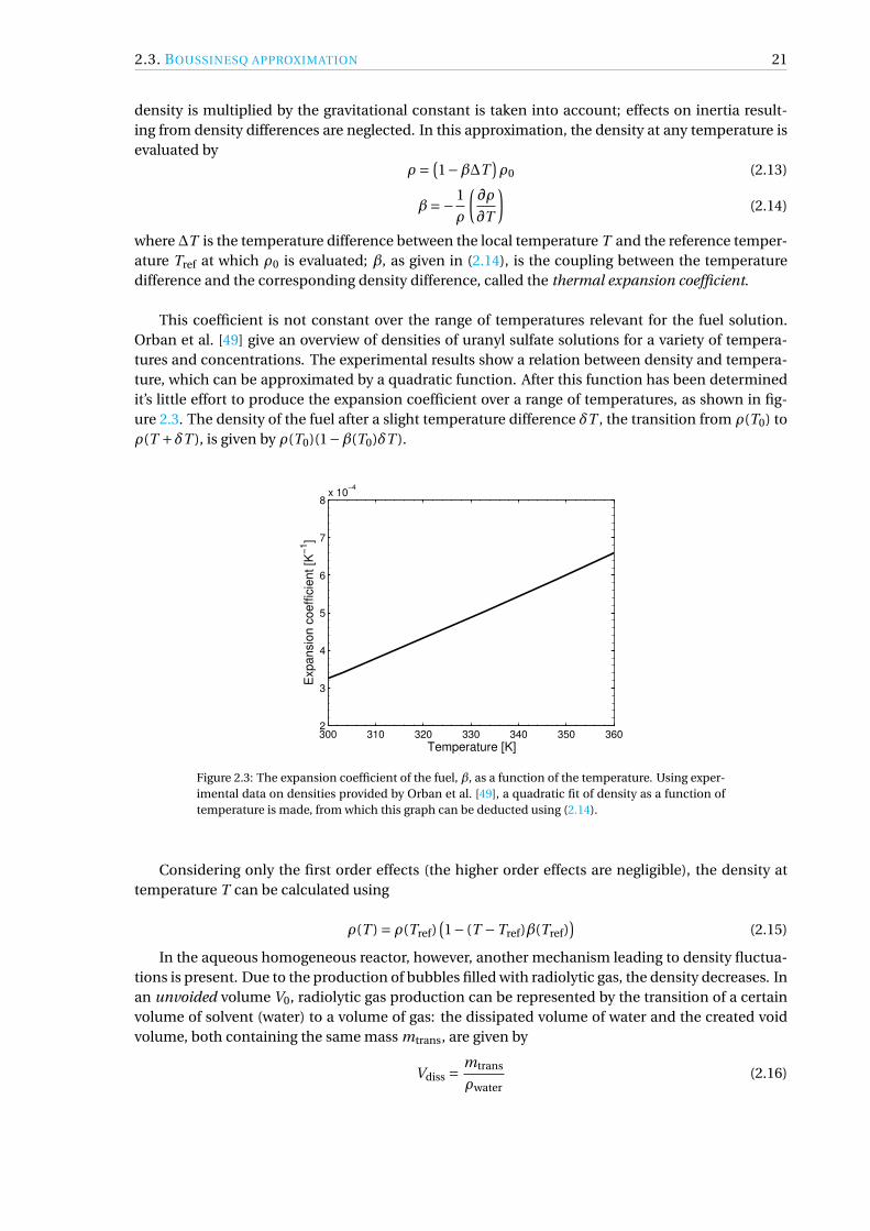
This coefficient is not constant over the range of temperatures relevant for the fuel solution.Orban et al. [49] give an overview of densities of uranyl sulfate solutions for a variety of tempera-tures and concentrations. The experimental results show a relation between density and tempera-ture, which can be approximated by a quadratic function. After this function has been determinedit’s little effort to produce the expansion coefficient over a range of temperatures, as shown in fig-ure 2.3. The density of the fuel after a slight temperature difference δT , the transition from ρ(T0) toρ(T +δT ), is given by ρ(T0)(1−β(T0)δT ).

300 310 320 330 340 350 3602

3

4

5

6

7

8x 10

−4

Temperature [K]

Exp

an

sio

n c

oe

ffic

ien

t [K

−1]

Figure 2.3: The expansion coefficient of the fuel, β, as a function of the temperature. Using exper-imental data on densities provided by Orban et al. [49], a quadratic fit of density as a function oftemperature is made, from which this graph can be deducted using (2.14).

Considering only the first order effects (the higher order effects are negligible), the density attemperature T can be calculated using

ρ(T ) = ρ(Tref)(1− (T −Tref)β(Tref)

)(2.15)

In the aqueous homogeneous reactor, however, another mechanism leading to density fluctua-tions is present. Due to the production of bubbles filled with radiolytic gas, the density decreases. Inan unvoided volume V0, radiolytic gas production can be represented by the transition of a certainvolume of solvent (water) to a volume of gas: the dissipated volume of water and the created voidvolume, both containing the same mass mtrans, are given by

Vdiss =mtrans

ρwater(2.16)

22 2. THEORY

Vvoid = mtrans

ρvoid(2.17)

The void fraction α can be calculated by dividing the void volume by the total volume

α= Vvoid

V0 −Vdiss +Vvoid(2.18)

which can be rearranged to give

Vvoid = αV0

(1−α)+α ρvoid

ρwater

(2.19)

V = V0

1+α(ρvoid

ρwater−1

) (2.20)

Equation (2.20) gives the ratio between the unvoided volume and the voided volume. Because den-sity is inversely proportional to volume, this expression can be used to write ρ as a function of ρ0

ρ =(1+α

(ρvoid

ρwater−1

))ρ0 (2.21)

Due to the fact that ρvoid << ρwater this boils down to

ρ = (1−α)ρ0 (2.22)

The analogy with equation (2.13) can easily be seen. Combining the thermal and void effects, thedensity can be calculated using

ρ = ρ0(1−β0∆T

)(1−α) ≈ ρ0(1−β0∆T −α) (2.23)

considering only first order effects.

For the traditional Boussinesq approximation, the correction factor β∆T should be small (β(T −Tref) << 1). With the temperature differences considered in this project, of the order of 20K and witha typical β of 5·10−4, this condition is fulfilled. Assuming a similar condition applies to the voidcorrection factor, the validity of (2.23) can be tested by looking at the void percentages. These are ofthe order 10−2 to 10−1, comparable to the values of β(T −Tref).

2.4. FUEL DENSITY CALCULATIONThe density of the fuel solution for an unvoided reactor at the reference temperature mainly de-pends on the concentration of uranyl salt dissolved. Following for the most part the method de-scribed by Sutondo [51], the procedure for calculation of the fuel density is shown in this part.

The fuel solution can be split into two general components; the salt and the water, each with itsown density. As the uranium concentration of the fuel usually is given, the amount of salt (in gL−1)present can be calculated by

csalt = cUMsalt

MU(2.24)

where M denotes the molar mass. The molar mass of uranium is a function of the enrichment, i.e.,the percentage of the lighter isotopes 234U and 235U. For an enrichment p, the weight fractions inuranium are given by

2.4. FUEL DENSITY CALCULATION 23

f(234U ) = 8.4400 ·10−3p −7.0084 ·10−4

f(235U ) = p (2.25)

f(238U ) = 1− f(235U ) − f(234U )

so the molar masses of this enriched uranium and of the salt are equal to:

MU = f(234U )M(234U ) + f(235U )M(235U ) + f(238U )M(238U )

Msalt =MU +6MO +MS (2.26)

With the molar mass and the density of the salt known, the volume fraction of the salt can easily beobtained using

vsalt =csalt

ρsalt= cU

ρsalt

Msalt

MU· 1

V(2.27)

where v is the volume fraction and V the total volume considered, in this case 1 dm3, which impliesthat the volume fraction of water is given by

vH2O = 1− vsalt (2.28)

This means the concentration of water can be written as

cH2O = vH2OV

ρH2O(2.29)

with ρ evaluated at the reference temperature. The density of the fuel for a certain concentration ofuranium can then be calculated using

ρfuel = vsalt ·ρsalt + vH2O ·ρH2O (2.30)

With the knowledge of the volumes occupied by the solute and solvent, the number densities canbe calculated in the following way:

N(234U ) =csalt

Msaltf(234U )NA

N(235U ) =csalt

Msaltf(235U )NA

N(238U ) =csalt

Msaltf(238U )NA

N(S) = csalt

MsaltNA

N(H) = 2cH2O

MH2ONA

N(O) = 6csalt

MsaltNA + cH2O

MH2ONA

with N(x) in dm−3.

24 2. THEORY

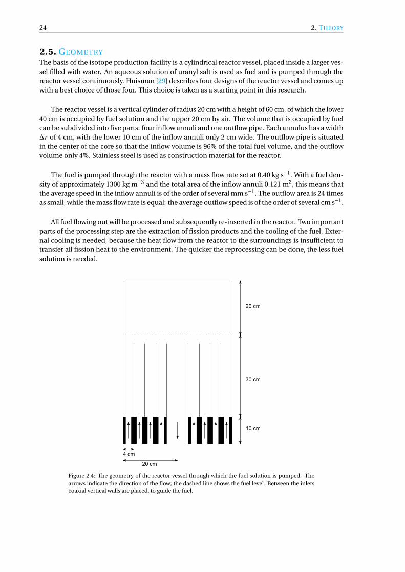
2.5. GEOMETRYThe basis of the isotope production facility is a cylindrical reactor vessel, placed inside a larger ves-sel filled with water. An aqueous solution of uranyl salt is used as fuel and is pumped through thereactor vessel continuously. Huisman [29] describes four designs of the reactor vessel and comes upwith a best choice of those four. This choice is taken as a starting point in this research.

The reactor vessel is a vertical cylinder of radius 20 cm with a height of 60 cm, of which the lower40 cm is occupied by fuel solution and the upper 20 cm by air. The volume that is occupied by fuelcan be subdivided into five parts: four inflow annuli and one outflow pipe. Each annulus has a width∆r of 4 cm, with the lower 10 cm of the inflow annuli only 2 cm wide. The outflow pipe is situatedin the center of the core so that the inflow volume is 96% of the total fuel volume, and the outflowvolume only 4%. Stainless steel is used as construction material for the reactor.

The fuel is pumped through the reactor with a mass flow rate set at 0.40 kg s−1. With a fuel den-sity of approximately 1300 kg m−3 and the total area of the inflow annuli 0.121 m2, this means thatthe average speed in the inflow annuli is of the order of several mm s−1. The outflow area is 24 timesas small, while the mass flow rate is equal: the average outflow speed is of the order of several cm s−1.

All fuel flowing out will be processed and subsequently re-inserted in the reactor. Two importantparts of the processing step are the extraction of fission products and the cooling of the fuel. Exter-nal cooling is needed, because the heat flow from the reactor to the surroundings is insufficient totransfer all fission heat to the environment. The quicker the reprocessing can be done, the less fuelsolution is needed.

30 cm

10 cm

20 cm

4 cm

20 cm

Figure 2.4: The geometry of the reactor vessel through which the fuel solution is pumped. Thearrows indicate the direction of the flow; the dashed line shows the fuel level. Between the inletscoaxial vertical walls are placed, to guide the fuel.

2.6. TEMPERATURE DISTRIBUTION AND COOLING 25

2.6. TEMPERATURE DISTRIBUTION AND COOLINGAn important safety characteristic of the reactor is the temperature distribution. Local boiling,caused by a high local temperature, can cause unwanted effects like slushing.

The water outside the reactor vessel is contained in a stainless steel tank (hereafter referred toas water vessel) and heats up due to the conduction of heat from the fuel through the wall of the in-ner vessel (referred to as reactor vessel). Induced by buoyancy effects, this water starts to circulate,hot parts moving upwards and cool parts downwards. By conduction of heat, the water vessel wallis heated, and when this wall has a temperature higher than the ambient temperature, the heat istransferred to the surrounding air.

To determine the amount of heat flow from the cylindrical wall to the surrounding air, knowl-edge about the heat transfer coefficient is essential. Useful information on this subject can be foundin the book Fundamentals of Momentum, Heat, and Mass Transfer [52]. A detailed explanation ofNusselt numbers for different geometries is given, from which the ones applicable to the aforemen-tioned configuration can be calculated.

An equation found by Churchill and Chu through investigation of experimental data can beused to calculate the Nusselt number for a vertical plate, but also for a vertical cylinder, providedthe dimensions of the cylinder dimensions obey the following condition

D

L≥ 35

Gr14

(2.31)

where D and L are the characteristic diameter and length (in this case the height), and Gr the Grashofnumber. The Churchill-Chu relation provides the Nusselt number as a function of both the Rayleighand the Prandtl number

Nu =

0.825+ 0.387Ra16(

1+ (0.492Pr

) 916

) 827

2

(2.32)

Aside from heat transfer from the vertical water vessel wall, the heat transfer from the circulartop (horizontal) of the water vessel has to be considered. The bottom is considered to be insulatedimplicating no heat flux occurs here. The relation for the Nusselt number for a horizontal plate iseasier than that for a vertical plate, but is different for different ranges of the Rayleigh number

Nu = 0.54Ra14 if 105 < Ra < 2 ·107 (2.33a)

Nu = 0.14Ra13 if 2 ·107 < Ra < 3 ·1010 (2.33b)

With the knowledge obtained about the Nusselt numbers and the geometrical properties, therelation between the total heat flow and the temperature difference (with T∞ the temperature faraway from the cylindrical water vessel) can be specified

q =(Nutop

λAtop

D+Nuside

λAside

L

)(T −T∞) (2.34)

As can be seen, the total heat flow is a function of the water vessel wall temperature T. In fig-ure 2.5, the total heat flow from the water vessel is shown as a function of the temperature of the

26 2. THEORY

wall of the water vessel, assuming a constant temperature of the surrounding air. With all other pa-rameters known, equation (2.34) can be solved using an iterative process, evaluating the materialproperties at a temperature referred to as the film temperature, which is the average of the watervessel wall temperature and the ambient temperature T+T∞

2 .

300 305 310 315 320 325 330 335100

200

300

400

500

600

700

800

900

1000

Wall temperature [K]

To

tal h

ea

t flo

w [

W]

Figure 2.5: The higher the temperature at the wall of the water container is, the larger the amountof heat flow from the reactor to the surroundings. This makes sense, because the temperaturedifference is the driving force for heat transfer. A small kink can be seen between 310 and 315 K.For higher temperatures the Rayleigh number is larger than 2·107, causing a change in the relationbetween the Nusselt and Rayleigh number (see (2.33)). The air temperature far away from thereactor is set at 298K.

3COMPUTATIONAL CODES

3.1. SCALE XSDRNPMThe multiplication factors for different fuel solutions as described in chapter 2.1 are calculated usingthe program SCALE. This program performs calculations regarding reactor physics and criticalityand is developed by Oak Ridge National Laboratory (ORNL). SCALE XSDRNPM is a one-dimensionalcode for neutron transport, and is used to calculate the multiplication factor keff for a specified ge-ometry. The atomic composition of the material is entered by defining the nuclides present togetherwith their number densities. For the calculations in chapter 2.1, the program uses the ENDF/B-Vcross section database, and solves the Boltzmann equation (3.1) for 238 energy groups. Using a S16

calculation with 30 inner and 20 outer iterations (for swift calculation and enough accuracy), thekeff and flux are calculated.

~Ω ·∇Ψ(~r ,E ,~Ω

)+Σt (~r ,E)Ψ(~r ,E ,~Ω

)= S(~r ,E ,~Ω

)(3.1)

This time-independent version of the Boltzmann equation (the keff, which arises in the fission sourceterm, will not change in time for a fixed geometry and composition) consists of four terms: the leak-age/flow term ~Ω · ∇Ψ, the interaction term ΣtΨ and two source terms (denoted by S). The fissionsource term can be written as

1

k

1

4πχ (~r ,E)

∫ 4π

0d~Ω′

∫ ∞

0ν

(~r ,E ′)Σ f

(~r ,E ′)Ψ(

~r ,E ′, ~Ω′)

dE ′

with ν the average number of neutrons produced per fission (approximately 2.45), Σ f the macro-scopic fission cross section, χ the fraction of the produced neutrons per unit energy and k the effec-tive multiplication factor.

The scatter source term ∫ 4π

0dΩ′

∫ ∞

0Σs

(~r ,E ′ → E , ~Ω′ →~Ω

)Ψ

(~r ,E ′, ~Ω′

)contains the macroscopic scattering cross section, specified for scattering from a certain energy and

direction(E ′, ~Ω′

)to

(E ,~Ω

).

3.2. HEATOne of the characteristic aspects of the designs of the AHRs discussed in chapter 2.5 is that thefuel is continuously flowing through the reactor. However, the flow of fuel is not the only process

27

28 3. COMPUTATIONAL CODES

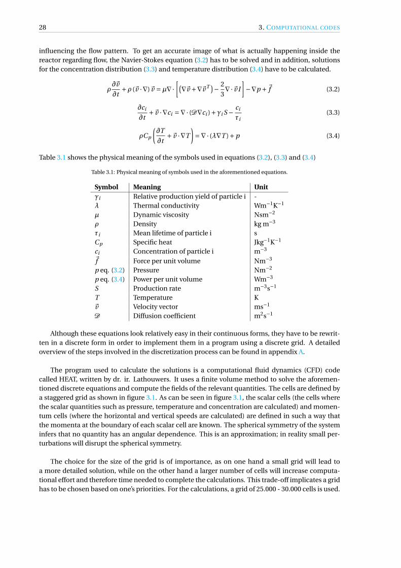
influencing the flow pattern. To get an accurate image of what is actually happening inside thereactor regarding flow, the Navier-Stokes equation (3.2) has to be solved and in addition, solutionsfor the concentration distribution (3.3) and temperature distribution (3.4) have to be calculated.

ρ∂~v

∂t+ρ (~v ·∇)~v =µ∇·

[(∇~v +∇~vT )− 2

3∇·~v I

]−∇p +~f (3.2)

∂ci

∂t+~v ·∇ci =∇· (D∇ci )+γi S − ci

τi(3.3)

ρCp

(∂T

∂t+~v ·∇T

)=∇· (λ∇T )+p (3.4)

Table 3.1 shows the physical meaning of the symbols used in equations (3.2), (3.3) and (3.4)

Table 3.1: Physical meaning of symbols used in the aforementioned equations.

Symbol Meaning Unitγi Relative production yield of particle i -λ Thermal conductivity Wm−1K−1

µ Dynamic viscosity Nsm−2

ρ Density kg m−3

τi Mean lifetime of particle i sCp Specific heat Jkg−1K−1

ci Concentration of particle i m−3

~f Force per unit volume Nm−3

p eq. (3.2) Pressure Nm−2

p eq. (3.4) Power per unit volume Wm−3

S Production rate m−3s−1

T Temperature K~v Velocity vector ms−1

D Diffusion coefficient m2s−1

Although these equations look relatively easy in their continuous forms, they have to be rewrit-ten in a discrete form in order to implement them in a program using a discrete grid. A detailedoverview of the steps involved in the discretization process can be found in appendix A.

The program used to calculate the solutions is a computational fluid dynamics (CFD) codecalled HEAT, written by dr. ir. Lathouwers. It uses a finite volume method to solve the aforemen-tioned discrete equations and compute the fields of the relevant quantities. The cells are defined bya staggered grid as shown in figure 3.1. As can be seen in figure 3.1, the scalar cells (the cells wherethe scalar quantities such as pressure, temperature and concentration are calculated) and momen-tum cells (where the horizontal and vertical speeds are calculated) are defined in such a way thatthe momenta at the boundary of each scalar cell are known. The spherical symmetry of the systeminfers that no quantity has an angular dependence. This is an approximation; in reality small per-turbations will disrupt the spherical symmetry.

The choice for the size of the grid is of importance, as on one hand a small grid will lead toa more detailed solution, while on the other hand a larger number of cells will increase computa-tional effort and therefore time needed to complete the calculations. This trade-off implicates a gridhas to be chosen based on one’s priorities. For the calculations, a grid of 25.000 - 30.000 cells is used.

3.2. HEAT 29

P(i,j)

P(i,j-1)

P(i-1,j)

P(i-1,j-1)

P(i-1,j+1)

P(i+1,j)

P(i+1,j+1)

P(i+1,j-1)

v(i,j) v(i+1,j)

v(i,j+1)

v(i-1,j)

P(i,j+1)

v(i-1,j+1) v(i+1,j+1)

u(i,j)

u(i,j+1)

u(i+1,j)

u(i+1,j+1)u(i-1,j+1)

u(i-1,j)

x

y

Figure 3.1: A part of the grid surrounding the scalar cell (i,j). The cells bounded by the green dashedlines and horizontal solid black lines are the horizontal (u) momentum cells, the cells confinedby the vertical solid borders and the red lines are the vertical (v) momentum cells and the cellsdenoted by P are the scalar cells.

As already mentioned, some assumptions are made in the calculations. First, although HEAThas been designed to deal with turbulent flows, turbulent effects are neglected during calculationsas the speeds in the reactor are relatively low, so that the flow is in the laminar regime. Second, thebuoyancy effects on the vertical momentum are approximated using the Boussinesq theorem (seesection 2.3) to describe density differences

ρ = (1−β0∆T

)ρ0 (3.5)

This approximation is valid if β∆T << 1. The temperature differences and the thermal expansionfactor in the reactor are of the order 101 and 10−4 (see figure 2.3) respectively, so this criterium isfulfilled. A third approximation is that all formed gas bubbles move at the same speed as the fuel,and therefore ca not escape from the fuel into the air above. The justification for this assumptionstems from the notion that the bubbles have a very small size and low speed relative to the fuel, ex-plained in section 2.2. Finally, the fuel level is set at a fixed height ignoring ripples, which is a validapproximation when the speeds are sufficiently low so that no slushing will occur.

For linking the pressure and velocity, a pressure-correction method called SIMPLE (Semi-ImplicitMethod for Pressure-Linked Equations) is used. A detailed explanation of this algorithm can befound in the book ‘An introduction to computational fluid dynamics’ [53]; globally it is an iterativesolving mechanism which updates pressure and speed turn by turn, until convergence is reached.

During the calculations on the steady state behavior of the reactor, another (outer) loop is cre-ated which, for a given power, updates all characteristics (momenta and pressure in the SIMPLE rou-tine and temperature) until a predefined level of temperature convergence is reached. Both loopsare shown schematically in figure 3.2.

30 3. COMPUTATIONAL CODES

Geometry

Grid

CalculateISpeeds

CalculateIPressures

Power

TemperatureIfield135XeIdistribution99MoIdistribution

VoidIdistribution

InitialItemperatureIfield

InitialI135XeIdistribution

InitialI99MoIdistribution

InitialIvoidIdistribution

Converged

NotIconverged

InitialIpressureIfield

PressureIfieldConverged

NotIconverged

Figure 3.2: A schematic overview of the flowchart of HEAT. The geometry, power and grid are usedto produce an initial guess for the fields that are going to be calculated. In a calculation of thesteady state these are put into a loop which recalculates the fields until a convergence criteriumis fulfilled. Inside this loop, another loop (the SIMPLE routine) is placed, which updates the mo-menta and pressure iteratively.

3.3. SERPENTAs HEAT calculates only the flow and temperature profile for a given power distribution, anothercode is needed to calculate the power distribution for a given temperature distribution. The neu-tronics part of the process is calculated by a code called Serpent, which is a continuous-energyMonte Carlo reactor physics code [54]. Development started in 2004 at the VTT Technical ResearchCentre of Finland under supervision of Jaakko Leppänen, and although the code is still being im-proved, it is already useful for finding a detailed power distribution. Based on the irradiation historyand a list of depleted materials together with a decay and a fission yield library, also the fuel burnupcan be calculated. For an increase in computational speed, the possibility of parallel processing isincluded, which is particularly useful because the Serpent calculations contribute a large part to thetotal calculation time.

In the evaluation, neutrons are simulated one by one travelling through the geometry definedby the input file. These neutrons interact with the materials, using the ENDF/B-VII database forevaluating cross sections. On the basis of these interactions, a power distribution is created, whichcontains information about the fission events and therefore the production of isotopes. Of coursethe simulation of more neutrons leads to a higher statistical accuracy, but again there is the impor-tant trade-off between accuracy and calculation time.

3.4. COUPLING BETWEEN SERPENT AND HEATIn order to calculate a steady state solution, HEAT and Serpent are coupled, because the neutronics(calculated with Serpent) are dependent on results from the fluid dynamics (calculated with HEAT)and vice versa. The coupling code transfers the calculated power distribution from Serpent to HEAT,and details on place-dependent fuel composition and temperature the other way around.

3.5. POINT KINETICS 31

HEAT

No temperatureconvergence

Temperatureconvergence

Serpent

Multiplicationfactor convergence

No multiplication factor convergence

k = 1

k ≠ 1

Steady State

New power guessGeometry

Initial power guessGrid

Core configuration

Figure 3.3: A schematic review of the flowchart for calculation of the steady state power. The firstloop is the HEAT loop as shown in figure 3.2. Subsequently, Serpent calculates the multiplicationfactor using the fields calculated in HEAT, in the scheme included as ‘core configuration’. If theouter loop has converged and the multiplication factor is not equal to 1, a new power guess ismade and the next outer loop iteration starts.

As the number of cells used in Serpent (800) is significantly smaller than the amount of cells inHEAT (several thousands) due to calculation time issues, each Serpent cell corresponds to multiple(parts of) HEAT cells. When data is transferred from HEAT to Serpent, the values (particle concen-trations, temperature) stored in the Serpent cells are the averages of the values in the correspondingHEAT cells. If data is transferred in the opposite way, the values calculated by Serpent (power den-sity, isotope production) in a single Serpent cell are stored in multiple HEAT cells.

In figure 3.3, the schematic program structure for finding the steady state power is shown. Everycalculation of the steady state power starts with a specification of the geometry accompanied by aninitial power density guess. In a number of iterations, HEAT calculates the flow profile, temperaturedistributions and fuel compositions; the loop is stopped when the temperature difference betweentwo subsequent iterations is smaller than a predefined value. If the temperature has converged, thefuel specifications of each HEAT cell are moulded into the correct input form for Serpent. If themultiplication factor calculated by Serpent is similar to the one calculated in a previous iteration(within a predefined radius of convergence), the power is changed (if keff > (1+ε) or keff < (1−ε),with ε defining the accuracy), or the loop is ended (if (1−ε) ≤ keff ≤ (1+ε)) and the steady statepower is found.

3.5. POINT KINETICSThe transient behavior of the reactor is very important for the safety evaluation. As long as thereactor operates at the steady state power and no events disrupting any parameter occur, the time-dependent evolution is rather predictable and slow. In case of an event, either wanted (caused byoperating personnel) or unwanted (system malfunction), various parameters are prone to change.Therefore, an assessment of various events and their consequences has to be made in order to iden-tify and subsequently eliminate or reduce certain risks.

The technique described before could be used, doing a Monte Carlo calculation for every timestep, but as each individual Monte Carlo calculation takes several hours to complete, this techniqueis not favorable for time-dependent calculations, in which several tens or hundreds of time steps areneeded. Therefore another method, point kinetics, is used to gain insight into the time evolution ofthe system properties.

32 3. COMPUTATIONAL CODES

The point reactor kinetics method makes use of a time-independent, spatial flux shapeψ, whichscales with an amplitude factor that is variable in time n(t). This assumption infers that point kinet-ics can be used as approximation as long as the flux shape change induced by perturbation of acertain parameter is not significant. An example of a case in which the spatial flux shape changessignificantly is for example the instantaneous removal of all fuel from the reactor core.

The point kinetics model uses seven different equations (of which 6 are quasi-identical)

dn

dt=

(ρ (t )−βΛ

)n (t )+Σiλi Ci (t ) (3.6a)

dC1

dt= β1

Λn (t )−λ1C1 (t )

... = ... (3.6b)

dC6

dt= β6

Λn (t )−λ6C6 (t )

where n is the previously mentioned amplitude factor, t the time, ρ the reactivity, β the delayedneutron fraction (βi is the delayed neutron fraction from the precursor group i), Λ the neutrongeneration time, λi the precursor decay constant and Ci the precursor concentration, both for thespecific group specified by i.

Implementing these equations, a prediction of the time evolution can be made, provided thatthe reactivity changes in time are known. An overview of reactivity effects resulting from a variety ofevents is given in chapter 5.

4STEADY STATE CALCULATIONS

4.1. INITIAL DESIGNAs a starting point for the development of the AHR, the exact same geometry as described by MarkHuisman (‘Bulkheads’) [29] is taken. The most significant difference in design is the fuel, which ischanged from a uranyl nitrate solution to a uranyl sulfate solution, with a uranium concentrationof 251 gL−1, flowing into the reactor at a rate of 0.4 kgs−1. Some additional changes were madein the code system, to better reflect actual physics; a method to calculate the void fraction due tothe production of radiolytic gas has been incorporated in HEAT. Furthermore, a scheme to describeexpansion of the fuel was added. This scheme corrects the local fuel composition for both tem-perature and void effects. The temperature expansion coefficient of water at 323 K was used in thecalculations. Fuel flows in at a temperature of 303 K, and the temperature at the reactor vessel wallis also fixed at 303 K.

Some characteristics of this reactor operating in steady state are visualized in figures 4.1 and 4.2.The thermal power of this reactor in a steady state situation is approximately 18.5 kW, with a higherpower density at the center of the reactor than at the outer regions. The power density (figure 4.1a)at the center of each inflow annulus is higher than that at the sides of the annulus. This is a result ofthe higher temperature and void fraction near the structural material, as can be seen in figures 4.1band 4.2a. Because the fuel speed decreases near the structural material (see figure 4.2b), the fuel willheat up more and the void fraction will increase. This will lead to a lower concentration of uraniumand therefore a lower power density. The temperature of the fuel stays well below the boiling point,the maximum temperature of 321.3 K is found in the outflow pipe at the center.

33

34 4. STEADY STATE CALCULATIONS

r [m]

z [

m]

0 0.1 0.2−0.1

0

0.1

0.2

0.3

Po

we

r d

en

sity [

Wm

−3]

0

1

2

3

4

5

6

7

8

9

10x 10

5

(a) The power density has roughly aspherical shape. In the middle of eachinflow annulus the power is somewhathigher than at the edges, which is mostevident in the most central inflow annu-lus

r [m]

z [

m]

0 0.1 0.2−0.1

0

0.1

0.2

0.3

T [

K]

295

300

305

310

315

320

(b) The temperature profile in the reac-tor. Temperature differences in the in-flow annuli arise for various reasons: thedifference in power density, differencein heat transfer to surrounding volume,and difference in flow speed.

Figure 4.1

r [m]

z [

m]

0 0.1 0.2−0.1

0

0.1

0.2

0.3

Vo

id f

ractio

n [

−]

0.02

0.04

0.06

0.08

0.1

0.12

0.14

(a) The void fraction near the guidingwalls tends to be higher than at otherplaces because of the low speed nearthese walls.

0 0.1 0.2−0.1

0

0.1

0.2

0.3

r [m]

z [

m]

|v| [m

/s]

0.00025

0.0006

0.0014

0.0034

0.008

0.019

0.045

0.11

(b) Looking closely at the flow pattern itcan be seen that the flow speed is lowerat the edges of the annulus.

Figure 4.2

4.2. ADJUSTING INFLOWBecause of the cylindrical core design, the inflow area of each annulus is dependent on the distancefrom the center of the reactor vessel. In the initial design the mass inflow rates for all annuli were allset at 25% of the total mass inflow rate, which led to higher fuel speeds in the center of the reactor.Although the power density is higher in this part of the reactor, the fuel is less irradiated because of

4.3. 12 INLETS 35

the high flow rate. The inflow ratios were changed to investigate the effect on the temperature, totalpower and void fraction, while keeping the total mass inflow rate at 0.4 kgs−1.

If the ratio between mass inflow rates is taken as the ratio of the areas of the inlet annuli per-pendicular to the flow (3:5:7:9), the fuel in the centre inflow annulus will heat up more, as the powerdensity is higher at the core of the reactor. To correct for this effect, the ratio (7:9:11:13) is chosen.

At a slightly lower power level (18.2 kW compared to 18.5 kW), the average temperature de-creases with 0.7 degrees whereas the maximum temperature increases by 1.6 degrees. The averagevoid fraction decreases with approximately 8% to 0.034.

The result of a higher temperature in the center and a lower temperature at the edge of thereactor vessel means less energy can be transferred to the environment. This will limit the totalpower at which the reactor operates in steady state.

r [m]

z [

m]

0 0.1 0.2−0.1

0

0.1

0.2

0.3

T [

K]

295

300

305

310

315

320

(a) Temperature

r [m]

z [

m]

0 0.1 0.2−0.1

0

0.1

0.2

0.3

Vo

id f

ractio

n [

−]

0.02

0.04

0.06

0.08

0.1

0.12

0.14

(b) Void fraction

r [m]

z [

m]

0 0.1 0.2−0.1

0

0.1

0.2

0.3

99M

o [

m−

3]

0

5

10

15x 10

16

(c) Concentration of99Mo

Figure 4.3: The inflow ratios have been changed from 1:1:1:1 to 7:9:11:13. As a result the tempera-ture in the most central inflow annulus is increased. Also the distributions of void and 99Mo havechanged in a similar way: an increase in the center annuli, a decrease in the outer ones.

4.3. 12 INLETSIn the initial design the flow speed in the center of the annuli is higher than at the sides, which leadsto an increased temperature and void fraction near the edges of the annuli. Furthermore, the abruptwidening at the inflow creates vortices in the bottom corners of the annuli (see figure 4.4a), whichalso cause a higher local void fraction and temperature. A local high void fraction should be avoided,because it can lead to the formation of larger bubbles which can, for example, cause slushing.

Both the previously mentioned effects can be prevented by splitting up each inlet into multipleinlets. By placing two inlets at the side and one at the center of each annulus, the flow speed near thestructural material is increased and the vortices have decreased in size, see figure 4.4b. In figure 4.5the vertical speed is shown as a function of the radius. The speed at the edge of each annulus is stillzero as it should be (because of the no-slip boundary condition), but the gradient is much steeper.

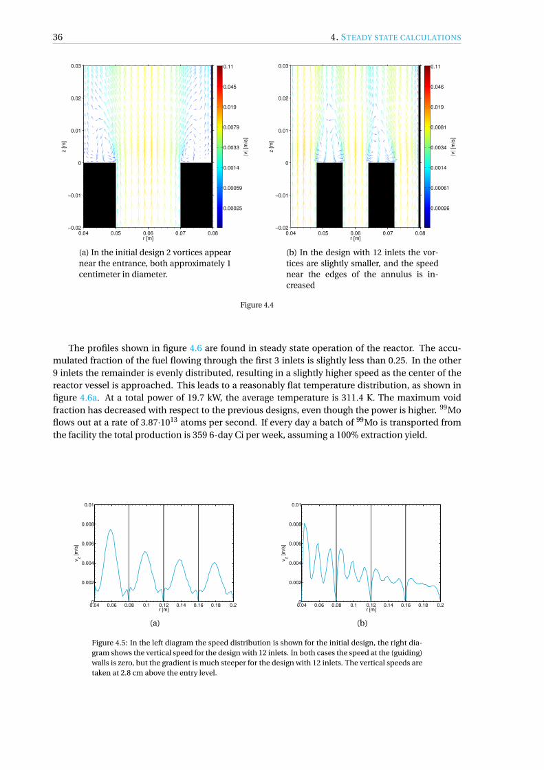
36 4. STEADY STATE CALCULATIONS

0.04 0.05 0.06 0.07 0.08−0.02

−0.01

0

0.01

0.02

0.03

r [m]

z [

m]

|v| [m

/s]

0.00025

0.00059

0.0014

0.0033

0.0079

0.019

0.045

0.11

(a) In the initial design 2 vortices appearnear the entrance, both approximately 1centimeter in diameter.

0.04 0.05 0.06 0.07 0.08−0.02

−0.01

0

0.01

0.02

0.03

r [m]

z [

m]

|v| [m

/s]

0.00026

0.00061

0.0014

0.0034

0.0081

0.019

0.046

0.11

(b) In the design with 12 inlets the vor-tices are slightly smaller, and the speednear the edges of the annulus is in-creased

Figure 4.4

The profiles shown in figure 4.6 are found in steady state operation of the reactor. The accu-mulated fraction of the fuel flowing through the first 3 inlets is slightly less than 0.25. In the other9 inlets the remainder is evenly distributed, resulting in a slightly higher speed as the center of thereactor vessel is approached. This leads to a reasonably flat temperature distribution, as shown infigure 4.6a. At a total power of 19.7 kW, the average temperature is 311.4 K. The maximum voidfraction has decreased with respect to the previous designs, even though the power is higher. 99Moflows out at a rate of 3.87·1013 atoms per second. If every day a batch of 99Mo is transported fromthe facility the total production is 359 6-day Ci per week, assuming a 100% extraction yield.

0.04 0.06 0.08 0.1 0.12 0.14 0.16 0.18 0.20

0.002

0.004

0.006

0.008

0.01

r [m]

vz [

m/s

]

(a)

0.04 0.06 0.08 0.1 0.12 0.14 0.16 0.18 0.20

0.002

0.004

0.006

0.008

0.01

r [m]

vz [

m/s

]

(b)

Figure 4.5: In the left diagram the speed distribution is shown for the initial design, the right dia-gram shows the vertical speed for the design with 12 inlets. In both cases the speed at the (guiding)walls is zero, but the gradient is much steeper for the design with 12 inlets. The vertical speeds aretaken at 2.8 cm above the entry level.

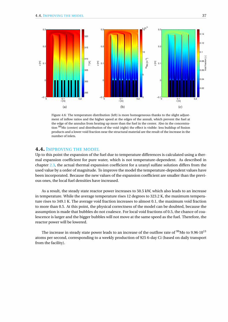
4.4. IMPROVING THE MODEL 37

r [m]

z [

m]

0 0.1 0.2−0.1

0

0.1

0.2

0.3

T [

K]

295

300

305

310

315

320

(a)

r [m]

z [

m]

0 0.1 0.2−0.1

0

0.1

0.2

0.3

99M

o [

m−

3]

0

5

10

15x 10

16

(b)

r [m]

z [

m]

0 0.1 0.2−0.1

0

0.1

0.2

0.3

Vo

id f

ractio

n [

−]

0.02

0.04

0.06

0.08

0.1

0.12

0.14

(c)

Figure 4.6: The temperature distribution (left) is more homogeneous thanks to the slight adjust-ment of inflow ratios and the higher speed at the edges of the annuli, which prevent the fuel atthe edge of the annulus from heating up more than the fuel in the center. Also in the concentra-tion 99Mo (center) and distribution of the void (right) the effect is visible: less buildup of fissionproducts and a lower void fraction near the structural material are the result of the increase in thenumber of inlets.

4.4. IMPROVING THE MODELUp to this point the expansion of the fuel due to temperature differences is calculated using a ther-mal expansion coefficient for pure water, which is not temperature-dependent. As described inchapter 2.3, the actual thermal expansion coefficient for a uranyl sulfate solution differs from theused value by a order of magnitude. To improve the model the temperature-dependent values havebeen incorporated. Because the new values of the expansion coefficient are smaller than the previ-ous ones, the local fuel densities have increased.

As a result, the steady state reactor power increases to 50.5 kW, which also leads to an increasein temperature. While the average temperature rises 12 degrees to 323.2 K, the maximum tempera-ture rises to 349.1 K. The average void fraction increases to almost 0.1, the maximum void fractionto more than 0.5. At this point, the physical correctness of the model can be doubted, because theassumption is made that bubbles do not coalesce. For local void fractions of 0.5, the chance of coa-lescence is larger and the bigger bubbles will not move at the same speed as the fuel. Therefore, thereactor power will be lowered.

The increase in steady state power leads to an increase of the outflow rate of 99Mo to 9.96·1013

atoms per second, corresponding to a weekly production of 925 6-day Ci (based on daily transportfrom the facility).

38 4. STEADY STATE CALCULATIONS

r [m]

z [

m]

0 0.1 0.2−0.1

0

0.1

0.2

0.3

T [

K]

300

310

320

330

340

350

(a)

r [m]

z [

m]

0 0.1 0.2−0.1

0

0.1

0.2

0.3

99M

o [

m−

3]

0

0.5

1

1.5

2

2.5

3

3.5

4x 10

17

(b)

r [m]

z [

m]

0 0.1 0.2−0.1

0

0.1

0.2

0.3

Vo

id f

ractio

n [

−]

0

0.05

0.1

0.15

0.2

0.25

(c)

Figure 4.7: Because the new expansion coefficient is much smaller than the one previously used,the total amount of uranium in the core has increased, causing an increase in the total power bya factor of approximately 2.5. This increase leads to higher temperatures (a), but the maximumtemperature stays well below the boiling point. Also the concentration of 99Mo (b) and the voidfraction (c) increase with a factor of approximately 2.5, leading to high void fractions (over 20%).

4.5. LOWERING THE CONCENTRATION

Because the production rate of 99Mo using a 251 gL−1 uranium solution exceeds 200 6-day Ci perweek and the power level causes large void fractions, the power will be lowered. An easy way to dothis is to lower the uranium concentration. Using a solution with 225 gL−1 uranium in the form ofa uranyl sulfate solution rather than the original solution leads to a steady state power of 13.6 kW.The maximum void fraction has decreased to 0.18, the average temperature to 308.4 K and the max-imum temperature to 316.5 K.

4.6. IMPROVING THE CODE 39

r [m]

z [

m]

0 0.1 0.2−0.1

0

0.1

0.2

0.3

T [

K]

295

300

305

310

315

(a)

r [m]

z [

m]

0 0.1 0.2−0.1

0

0.1

0.2

0.3

99M

o [

m−

3]

0

1

2

3

4

5

6

7

8

9

10x 10

16

(b)

r [m]

z [

m]

0 0.1 0.2−0.1

0

0.1

0.2

0.3

Vo

id f

ractio

n [

−]

0

0.01

0.02

0.03

0.04

0.05

0.06

0.07

0.08

0.09

0.1

(c)

Figure 4.8: By lowering the concentration of uranium, the power of the reactor decreases drasti-cally. As a result, the fuel heats up significantly less, leading to a maximum temperature of only316.5 K. Also the molybdenum concentration and the void fraction decrease.

4.6. IMPROVING THE CODEUntil now, all calculations have been performed with a fixed temperature at the boundary of thefuel region, which of course does not reflect the actual situation. In a few steps the code has beenextended to include temperature gradients, pressure differences and buoyancy-driven flows in thewater vessel. As a first step, the temperature at the inside of the water vessel wall is set to a fixedvalue. This enables temperature differences (figure 4.9b) in both air and water regions, leading tobuoyancy-driven flows. However, the temperature at the boundary of the water vessel is not theboundary value. In chapter 2.6, a correlation between the heat flow and both the water vessel walltemperature and the surrounding air temperature is shown. Adding an iterative loop, this conditioncan be used to accurately determine the temperature distribution in the entire reactor, shown infigure 4.9c. The buoyancy-driven flows and the flow pattern of the fuel are shown in figure 4.11.

Because the temperature at the outer boundary of the system is increased with respect to pre-vious calculations, the heat transfer has deteriorated. As a result, the power is slightly lowered (13.2kW), leading to a maximum fuel temperature of 316.1 K; well below the boiling temperature. Theaverage 99Mo concentration at the outflow is 9.44·1016 m−3, which equals a production of 266 6-dayCi per week, assuming a 100% extraction yield and daily transport from the facility.

40 4. STEADY STATE CALCULATIONS

r [m]

z [

m]

0 0.1 0.2 0.3−0.1

0

0.1

0.2

0.3

0.4

0.5

0.6

T [

K]

295

300

305

310

315

(a)

r [m]

z [

m]

0 0.1 0.2 0.3−0.1

0

0.1

0.2

0.3

0.4

0.5

0.6

T [

K]

295

300

305

310

315

(b)

r [m]

z [

m]

0 0.1 0.2 0.3−0.1

0

0.1

0.2

0.3

0.4

0.5

0.6

T [

K]

295

300

305

310

315

(c)

Figure 4.9: The temperature of the water in the water vessel has been fixed at 293 K. Because thewater temperature does not rise, the temperature gradient will be overestimated, which results ina larger heat transfer than in reality (a). In another case, the temperature of the water vessel wallhas been fixed at 293 K. The air above the fuel can only conduct heat, so the heat transfer is un-derestimated (b). Finally, both the water and air region can flow as a result of density differences,leading to a more realistic heat transfer. The heat transfer from the wall to the environment is afunction of the wall temperature and the ambient temperature, which is set at 293 K (c).

0 0.08 0.16 0.24 0.32290

295

300

305

310

315

320

r [m]

T [K

]

0 0.08 0.16 0.24 0.32290

295

300

305

310

315

320

r [m]

T [K

]

(a)

(b)

(c)

(a)

(b)

(c)

Figure 4.10: The radial temperature distribution in the left figure is taken at z = 0.2 m, in the rightfigure at z=0.3m. Cases (a), (b) and (c) correspond to figures 4.9a, 4.9b and 4.9c respectively. Incase (a) the most heat can be transferred, which can be seen from the temperature difference atthe side of the reactor (r = 0.2 m) and at the top, where the temperature difference is largest in case(a).

4.6. IMPROVING THE CODE 41

0 0.1 0.2 0.3−0.1

0

0.1

0.2

0.3

0.4

0.5

0.6

r [m]

z [m

]

|v| [

m/s

]

0.00027

0.00063

0.0015

0.0035

0.0084

0.02

0.047

0.11

Figure 4.11: The flow pattern of the air, water and fuel in one figure. The flow of the water and airis caused by buoyancy effects; the dashed ellipses indicate the circulation of the fluids.

5REACTIVITY ANALYSIS

For investigating the time-dependent behavior of the reactor, a database of reactivity effects is as-sembled. Seven parameters are looked into: uranium concentration, 135Xe concentration, void frac-tion, fuel temperature, fuel level (an increase in the height of the fuel in the reactor core), water level(a decrease of the level of the water in the water vessel) and a fuel leak (a leak of fuel from the reactorinflow pipe to the water in the water vessel). The time-dependent reactivity value used in transientcalculations will be a sum of these individual reactivity effects.

Serpent is used to calculate the effective multiplication factor for every perturbation of thesteady state. All parameters are perturbed multiple times individually, so that a database of mul-tiplication factors corresponding to perturbed situations is available. Subsequently, the reactivityρ = k−1

k is calculated and a function is fitted to be able to interpolate the data, which is necessaryfor the point kinetics calculations.

In some transient calculations, the reactivity value used in the calculations is a sum of the in-dividual reactivity effects, which is only accurate if no correlation between effects exists. To see ifour data fulfills this requirement, Serpent is used once again to calculate the reactivity in a situationwhere multiple characteristics are changed simultaneously.

43

44 5. REACTIVITY ANALYSIS

5.1. URANIUM CONCENTRATIONIf the uranium concentration in the fuel increases, the macroscopic absorbtion cross section (es-pecially fission) of the fuel increases and the non-leakage probability of a neutron increases, whichmeans the multiplication factor increases. The relation between the uranium concentration andthe reactivity is shown in figure 5.1. A second order correlation is used to fit the datapoints, whichhas uncertainties of approximately 8 pcm.

The reactivity as function of the uranium concentration is represented by

ρU =−4.3417 ·10−6c2U +2.9077 ·10−3cU −4.3443 ·10−1 (5.1)

which corresponds to a reactivity effect of 95.4 pcm (gL−1)−1 at a uranium concentration of 225gL−1. Huisman has found a reactivity of 66.0 pcm (gL−1)−1 for his uranyl nitrate fueled design ata uranium concentration of 248 gL−1. A similar value (75.4 pcm (gL−1)−1) is found for the currentdesign with the uranium concentration set at 248 gL−1.

200 210 220 230 240 250 260 270 280−4000

−3000

−2000

−1000

0

1000

2000

3000

4000

Concentration U [g L−1

]

Reactivity [pcm

]

Figure 5.1: The second order fit corresponds well to the data. All data points have error bars, butbecause the uncertainty is small with respect to the reactivity changes, these are not visible.

5.2. XENON CONCENTRATION135Xe is a known for its large neutron absorbtion cross section, so the evolution of the xenon con-centration plays a role in the transient behavior of the reactor. To analyse the effect of the xenonconcentration on the reactivity, the average concentration of xenon is increased and the reactivitiesare plotted. For a hundredfold increase of the xenon concentration the reactivity is -17 pcm, whichis of the same order of magnitude as the value found by Huisman [29].

The small effect on the reactivity can be explained by looking into the ratio of the number ofneutrons absorbed in the fuel material to the total number of neutrons absorbed (called the ther-

mal utilization factor, f = ΣFaΣa

, with Σa the macroscopic absorbtion cross section and superscript F

denoting ‘fuel’). If the macroscopic absorbtion cross section of 135Xe is only a small fraction of thetotal macroscopic absorbtion cross section, a hundred-fold increase in the concentration will causea small decrease of the thermal utilization factor and therefore a small decrease of the multiplica-tion factor. A second order fit to the data is shown in figure 5.2.

5.3. VOID FRACTION 45

100

101

102

103

−160

−120

−80

−40

0

40

135Xe/

135Xe

ref [−]

Reactivity [pcm

]

Figure 5.2: The reactivity effect of the 135Xe concentration divided by the concentration duringsteady state operation. A second order fit is made, and a logarithmic scale is used to show thereactivity at higher concentrations.

5.3. VOID FRACTIONIn steady state, the reactor operates with a void fraction of 0.0269. The larger this void fractionbecomes, the less volume is actually occupied by fuel. Therefore, a larger void fraction results in alower multiplication factor because a larger fraction of neutrons will leak from the reactor. Since thevoid fraction is proportional to the reactor power, an increase in power will lead to an increase of thevoid fraction, which will lower the reactivity (see figure 5.3). This negative feedback has a limitingeffect on the reactor power.

0.8 0.9 1 1.1 1.2 1.3−200

−150

−100

−50

0

50

100

150

200

Void/Voidref

[−]

Reactivity [pcm

]

Figure 5.3: For the reactivity effect of the void concentration, data for small perturbations is fitted.Whereas for the xenon concentration it was reasonable to look at a hundred-fold increase, it is notfor the void fraction. For large void fractions, the model will not represent reality as the modelassumes all void is present in the form of small bubbles.

5.4. TEMPERATUREThe temperature effect on the reactivity is a combined effect of Doppler broadening and the expan-sion of the fuel (for an increase in temperature). Using the Boussinesq approximation as presentedin chapter 2.3, an estimate of the expansion of the fuel is made, while the Doppler broadening isrealised by using cross sections at a different temperature. If a second order fit is made (see fig-ure 5.4) and the derivative is taken at a temperature of 310 K, a reactivity coefficient of -10 pcm K−1

is found, which is of the same order of magnitude as the value found by Cooling et al. for theirAHR, -19.2 pcm K−1 [46]. The reactivity effect is 3 times larger than the value provided by Huisman(-3.8 pcm K−1), who neglected expansion effects [29].

46 5. REACTIVITY ANALYSIS

300 305 310 315 320 325 330 335 340 345 350−600

−500

−400

−300

−200

−100

0

100

Average temperature [K]

Re

activity [

pcm

]

Figure 5.4: The negative temperature coefficient of reactivity is an important feedback mechanismof the AHR, and is shown above. Average temperatures up to 350 K are used for the fit, because themaximum temperature should stay below the boiling point.

5.5. REFLECTOR WATER LEVELIf the water level in the water vessel drops as a result of a leak, the reactor loses (part of) the reflector,leading to an increased fraction of neutrons leaking from the reactor which will reduce the multi-plication factor. Looking at the data, two regimes can be distinguished; therefore the fit of the datais split into two parts, see figure 5.5. Loss of the upper 30 centimeter of water will mainly affect theleakage from the top of the reactor, whereas loss of the lower 40 centimeter will influence mainlyleakage through the side wall of the reactor vessel. The latter has an area that is 4 times as big asthe top of the reactor. A decrease of the water level by one centimeter yields a decrease in reactivityof approximately 146 pcm when the water level is under 30 cm; for the upper part the effect is oneorder of magnitude smaller: approximately 15 pcm cm−1.

As mentioned in section 3.5, the point kinetics model assumes that the flux changes only in am-plitude. To check whether the change of the flux resulting from a decrease in water level fulfills thisrequirement, a plot (see figure 5.6) of the flux profile as function of the radius is made for a waterlevel of 60 cm and 0 cm. The flux level is simular in both situations because the total flux is normal-ized to the same value for both calculations. However, from the plot it becomes clear that the fluxprofile changes in the transition from a reflected reactor to a bare reactor. As expected, the relativeflux at the edge of the reactor is much smaller for a bare reactor than for a reflected reactor.

Although the requirement that the flux only changes in amplitude is not met, the point kineticsmodel will be used to calculate the transient behavior in case of a decrease of the reflector waterlevel.

5.6. FUEL LEVEL 47

−10 0 10 20 30 40 50 60−7000

−6000

−5000

−4000

−3000

−2000

−1000

0

1000

Rea

ctiv

ity [p

cm]

Water level [cm]

Figure 5.5: The fit of the data is split up into parts: the water part next to the fuel region showsa stronger reactivity coefficient. Where the two fits meet is a kink, which is a non-physical phe-nomenon, a consequence of evaluating the data as two different sets.

0 0.1 0.2 0.30

1

2

3

4

5x 10

12

r [m]

Flu

x [# c

m−

2s

−1]

Water level 60 cm

Water level 0 cm

Figure 5.6: The plot above shows the scalar neutron flux profile as a function of the radius, evalu-ated at z = 10 cm. When the water is at the normal level (60 cm), the relative flux near the boundaryis higher than when the water level has decreased to 0 cm, because the number of reflected neu-trons is higher.

5.6. FUEL LEVELAn increase in the fuel level results in a larger amount of uranium in the reactor core, presumingthe average uranium concentration does not change. If the volume is increased, the non-leakageprobability of a neutron is increased, causing a positive reactivity effect. Figure 5.7 shows a secondorder fit of the data points, which is used to calculate time-dependent reactivity values.

The larger fuel volume leads to a flux profile that is a little more spread out, as shown for threefuel levels in figure 5.8. Again the flux is normalized to the same value in the three calculations,leading to a similar amplitude.

48 5. REACTIVITY ANALYSIS

28 29 30 31 32 33 34 35−2000

−1000

0

1000

2000

3000

4000

Fuel height [cm]

Re

activity [

pcm

]

Figure 5.7: The fuel level has a large influence on the reactivity. This makes sense, because a 4cm rise of the fuel level means the fuel volume is increased by 10%, which means the amount ofuranium in the core is also increased by roughly 10%.

−0.1 0 0.1 0.2 0.3 0.4 0.5 0.60

1

2x 10

12

z [m]

Flu

x [# c

m−

2s

−1]

Fuel level 30.3 cm

Fuel level 31.5 cm

Fuel level 33 cm

Figure 5.8: A higher fuel level leads to a changed flux profile; the flux is stretched somewhat in thevertical direction (shown on the horizontal axis). Because the flux is normalized to the same valuefor the three cases, a stretched flux leads to a lower maximum value.

5.7. FUEL CONCENTRATION IN PART OF THE WATERIn this section, a leak at the most central inflow pipe of the reactor vessel is assumed, causing asmall concentration of uranium in the surrounding water. This will lead to an increase in power,because also fissions in the surrounding water will occur. To limit the amount of fuel solution inthe water and the spreading of this fuel, the water can be kept in various compartments to preventdiffusion and convection of leaked fuel. Another option is to keep the pressure in the water outsidethe reactor core higher than the pressure of the solution in the reactor, in which case a leak in thereactor vessel will cause water to flow into the core, rather than fuel flowing out. In figure 5.9 thereactivity is shown for fuel leaking out of the most central reactor inflow pipe into the water directlyaround it (enclosed by the two most central inflow pipes). Because of the circular symmetry of thecode, a leak will always be assumed circular.

5.8. LINEARITY OF FEEDBACK EFFECTS 49

0 0.05 0.1 0.15 0.2 0.25 0.3 0.35−30

−20

−10

0

10

20

30

40

Volume fraction fuel in water [−]R

eactivity [

pcm

]

Figure 5.9: Fuel is assumed to only flow into the volume enclosed by the two inner inflow pipes.Although many data points are taken, the trend is not really clear. A linear fit is used as approxi-mation for the data points, with an additional restriction for the fit to pass through (0,0).

5.8. LINEARITY OF FEEDBACK EFFECTSA last step is the investigation of the mutual dependence of the reactivity coefficients. If there is nocorrelation, the total reactivity can be written as

ρ = ρ0 +Σiρi (5.2)

with ρ0 the initial reactivity, and ρi the reactivity changes resulting from the various possible events.To investigate the linearity of the reactivity effects, multiple events are simulated at once. Serpent isused to calculate the reactivity, which is then compared to the sum of the reactivities of the separateevents. If no correlation between the effects exists, these values will be similar.

Looking at the values calculated by Serpent and the expectation based on addition of reactiv-ities using (5.2) (available in appendix B for reference), it can be noted that there is no correlationbetween effects for all events considered except for one case. An increase in fuel level and a decreasein water level re-enforce each other, leading to a larger increase in reactivity than is expected fromaddition of the effects. Therefore, no events in which both the fuel level and the water level changehave been considered in calculating the transient behavior.

Although the fit from section 5.7 does not seem to represent the data very well, the fit is usedin calculation of the combined effects. It is worth noticing that calculation of the reactivity by Ser-pent in case of simultaneous perturbation of multiple parameters including the concentration ofuranium in the surrounding water yields results which are consistent with the expected value cal-culated using (5.2).

6TRANSIENT CALCULATIONS

Starting from the steady state situation as described in chapter 4.6, the transient behavior of the re-actor is assessed for some events which are deemed probable. These include changes in the inflowconditions (uranium concentration, temperature of the fuel, flow rate), changes in ambient tem-perature and changes in the fuel and water level. The reactivity coefficients from chapter 5 are con-verted to a reactivity value, which is a function of time. With this value, the point kinetics equations(3.6a) and (3.6b) are solved. The neutron generation time in steady state operation Λ = 6.1662·10−5

s, the total delayed neutron fraction β = 7.5891·10−3. Other parameters that have to be put in tothe equations are listed in table 6.2. These values are available from the Serpent calculation of thesteady state situation.

Table 6.1: The group constants as used in the transient calculations, calculated by Serpent.

Group β λ [s−1] t 12

[s]

1 2.447·10−4 1.249·10−2 55.492 1.269·10−3 3.182·10−2 21.793 1.225·10−3 1.094·10−1 6.3354 3.471·10−3 3.172·10−1 2.1865 1.021·10−3 1.354 0.51216 3.582·10−4 8.649 0.0801

6.1. DELAYED NEUTRON FRACTIONThese values for β, however, are calculated without considering that precursors flow out of the core.Assuming an average fuel residence time of 30 seconds, it is likely that part of the precursors (espe-cially those with longer half-life) will decay outside the reactor vessel. Because neutrons released indecay of these precursors are not likely to induce a fission in the reactor vessel, the group constantsof groups one to three are changed. The groups with a short half-life time are not affected by thisassumption, as almost all precursors will decay before they flow out of the reactor.

Following the assumption that a precursor either decays in the core or flows out after 30 seconds,it can be calculated that the chance at decay inside the reactor for a precursor from group 1 is 41.8%,while for precursors in group 2 and 3 the chances are 74.8% and 99.1% respectively. The adaptedgroup constants βa are calculated by multiplying the group constant calculated by Serpent by thechance at decay inside the reactor vessel. The difference between the original β and the adapted

51

52 6. TRANSIENT CALCULATIONS

value βa is 6.3%.

Table 6.2: The adapted group constants, calculated using βa,i = Pi(decay

) ·βi with Pi(decay

)the

chance that a precursor from group i decays inside the reactor vessel.

Group βa λ [s−1] t 12

[s]

1 1.023·10−4 1.249·10−2 55.492 9.492·10−4 3.182·10−2 21.793 1.210·10−3 1.094·10−1 6.335

Two time evolutions starting from the steady state (starting with ρ = -1 pcm) have been calcu-lated, one with the original value for β and one with the adapted value. As can be seen in the leftgraph in figure 6.1, the change in the delayed neutron fraction leads to difference in reactivity. Thesmaller fraction of delayed neutrons results in a more prompt reactor behavior, as can be seen bythe shift of the curve to the left. The power, shown in the right diagram of figure 6.1, is not much dif-ferent for the two values of β; the maximum difference between the two cases is only 0.05%. Basedon these arguments, the original values of β are used in the transient calculations.

0 100 200 300 400 50013.1

13.2

13.3

timen[s]

Tot

alnp

ower

n[kW

]

0 100 200 300 400 500−1

−0.8

−0.6

−0.4

−0.2

0

0.2

0.4

0.6

timen[s]

ρ[p

cm]

AdaptednβOriginalnβ

AdaptednβOriginalnβ

Figure 6.1: The reactivity in pcm as a function of time for the original and the adapted delayedneutron fraction. As the delayed neutron fraction decreases, the reactor reacts more promptlyto changes, which is the cause of the steeper curve in case of an adapted value of β. The powervariations are induced by the reactivity changes; for the smaller value of β the power changes areslightly larger, but the difference between the two situations is negligible.

6.2. URANIUM CONCENTRATIONIn the reprocessing step, the fuel has to be prepared for a new cycle through the reactor. Assum-ing all fission products and radiolytic gases are extracted, only the uranyl sulfate and water remain.These have to be cooled, and the uranium concentration has to be set to 225 gL−1. An error in theuranium concentration could lead to problems, due to the large reactivity coefficient of the uraniumconcentration, as discussed in chapter 5.1. An increase of the inlet concentration to 227 gL−1 is sim-ulated, keeping all other parameters constant.

In approximately 300 seconds, the average uranium concentration in the reactor rises to its equi-librium level of 227 gL−1. Because of the higher uranium concentration, the reactivity rises to 25pcm, resulting in an increase in power. This leads to an increase in temperature, concentration

6.3. INFLOW RATE 53

0 100 200 300 400 50010

12.5

15

17.5

20

Pr[k

W]

0 100 200 300 400 500−50

−25

0

25

50

Rea

ctiv

ityr[p

cm]

0 100 200 300 400 500308

309

310

311

312

Tr[K

]

tr[s]0 100 200 300 400 500

224

225

226

227

228

Ave

rage

rcon

cent

ratio

nrU

r[g/L

]

tr[s]

Figure 6.2: An increase in the uranium concentration will lead to an increase in reactivity. Thisleads to an increase in the power, which results in an increase of the temperature. Eventually (att ≈ 300 s) the reactivity effects of the changed temperature, 135Xe concentration and void fractionwill cancel out the increase in reactivity from the increased uranium concentration.The new steadystate power is 18.2 kW

of 135Xe and the average void fraction. All these events decrease the reactivity, which eventuallybecomes zero. The reactor now operates at a new steady state power of 18.2 kW, with an averagetemperature of 310.2 K

6.3. INFLOW RATEAnother parameter that could be set to a wrong value is the flow rate. In the reference situation,the inflow rate is set at 0.4 kgs−1. If the inflow rate is lowered to 0.3 kgs−1, the outflow rate will alsodecrease to 0.3 kgs−1. This decrease in flow means that the fuel will spend more time in the reactor.Initially the power is at the steady state value, 13.2 kW. Because of the longer residence time the av-erage fuel temperature, void fraction and 135Xe concentration will rise. This will lead to a decreaseof the reactivity, which in turn leads to a decrease in power. As the power decreases more and more,the fuel temperature, void fraction and 135Xe concentration will drop again, resulting in a rise of thereactivity. After approximately 250 seconds the power settles at the new equilibrium level of 10.1 kW.

The inflow rate can also be set to a higher value than the 0.4 kgs−1. An increased inflow ratewill yield opposite effects from a decreased inflow rate. The fuel will flow faster, meaning it has lesstime to heat up. Also there is less buildup of fission products and radiolytic gas, leading to a positivereactivity. This positive reactivity results in an increase of the power, causing the temperature, 135Xeconcentration and void fraction to return to their equilibrium values. Figure 6.3 shows the develop-ment of both the total reactor power and temperature.

54 6. TRANSIENT CALCULATIONS

0 100 200 300 400 5008

10

12

14

16

18

20

t [s]

Tota

l pow

er

[kW

]

0 100 200 300 400 500308

308.5

309

309.5

t [s]

T [K

]

0.3 kg s−1

0.5 kg s−1

0.3 kg s−1

0.5 kg s−1

Figure 6.3: These graphs illustrate the power and temperature changes resulting from a changedinflow rate. If the inflow rate is increased (black), the power will initially rise, while the averagetemperature drops. For a decreased inflow rate (blue), the effects are reversed; the power initiallyincreases and the temperature decreases. After approximately 300 seconds, the power has settledat a new steady state level.

6.4. NO INFLOW

The fuel is pumped through the reactor core, and stops flowing when the pump stops. In that case,there is neither inflow nor outflow, so the fuel will spend a longer time in the reactor core. Thecooling by the water is not sufficient to transport all extra heat to the surroundings, so the fuel tem-perature will increase. Also, the void fraction and 135Xe concentration will increase because no freshfuel is pumped into the core. These three effects lead to a reduction of the reactivity, which is largeenough to stop the reactor (P = 0). When the power is almost at zero, the temperature starts to de-crease gradually because heat is transferred to the environment. The void fraction stays at the samelevel, because the code does not support void escaping from the fuel. In reality, however, the voidbubbles will rise to the surface of the fuel. Due to decay of 135I, the 135Xe concentration will initiallyincrease. After approximately 2.5 hours the average temperature of the fuel is decreased to the samelevel as before the inflow stopped (see figure 6.4).

0 1000 2000 3000 4000 5000

309

310

311

312

t [s]

T [

K]

0 1000 2000 3000 4000 50000

3

6

9

12

15

P [kW

]

t [s]0 1000 2000 3000 4000 5000

−500

−400

−300

−200

−100

0

Reactivity [pcm

]

Figure 6.4: If the fuel flow is stopped, a large negative reactivity is introduced as a result of theincrease of the void fraction, 135Xe concentration and temperature. After approximately 200 sec-onds, the temperature will decrease due to heat transfer through the reactor vessel wall, the voidand xenon however stay in the fuel and cause the reactor to shut down.

6.5. NO COOLING 55

6.5. NO COOLINGBecause the heat transfer from the reactor to the surroundings is insufficient to dissipate all fissionheat, the fuel is cooled externally after it has left the core. In case of a failure of the cooling system,the fuel will be reinserted in the reactor at a higher temperature. Even when the heat exchange sys-tem fails the fuel temperature will decrease somewhat before it is reinserted, but to be conservativefor calculating the transient the inflow temperature is set equal to the outflow temperature.

The average temperature will increase because of the high inflow temperature, causing a nega-tive reactivity. This causes the power to decrease, which limits the temperature rise. Furthermore,the decreasing power induces a decrease in 135Xe concentration and void fraction, which has a pos-itive effect on the reactivity, limiting the drop of the power. The average temperature, shown infigure 6.5, rises to approximately 356.3 K while the maximum temperature of the fuel stays at 359.9K which is well below the boiling point (the boiling point of an aqueous solution is always higherthan the boiling point of pure water [55]). Considering the fact that this calculation is conservative,it can be stated that safe operation is ensured in the event of loss of external cooling.

0 2000 4000 6000300

310

320

330

340

350

360

t [s]

T [

K]

0 2000 4000 60000

5

10

15

P [kW

]

t [s]0 2000 4000 6000

−20

−10

0

10R

ea

ctivity [pcm

]

Figure 6.5: The increasing fuel temperature creates a negative reactivity, which causes the power todecrease. As a result the production of void and 135Xe diminishes, leading to an increase in reac-tivity. Eventually, the effects cancel each other out at a power of 2.94 kW. The average temperatureat this power level is lower than 360 K.

6.6. INCREASE IN AMBIENT TEMPERATUREUntil now, all described transients scenarios result from flaws in either the fuel processing or theinflow conditions. However, changes in external parameters can also affect the reactor. The ambi-ent temperature is important for the heat transfer from the reactor vessel to the surroundings. Thehigher the ambient temperature, the less efficient the cooling of the reactor vessel. To investigatethe impact of a deteriorated heat transfer from the reactor, the ambient temperature is increasedfrom 293 K to 313 K.

As it turns out, the 20 K increase in ambient temperature does not have a large influence on thereactor characteristics. The amount of heat that is transferred from the fuel to the surroundings willdecrease slightly, but the influence on the average temperature is negligible. Initially, the power willfluctuate a little, because the initial reactivity is slightly less than 0.

56 6. TRANSIENT CALCULATIONS

0 100 200 300 400 500 600308

308.25

308.5

308.75

309

t [s]

T [K

]

0 100 200 300 400 500 60013

13.125

13.25

13.375

13.5

P [kW

]

t [s]0 100 200 300 400 500 600

−1

−0.5

0

0.5

1

Re

activity [pcm

]

Figure 6.6: Initially, the reactivity is negative, which leads to a small decrease in power. This in-duces an increase in reactivity resulting from void, temperature and 135Xe feedback. The reactivitythen slightly overshoots, which causes the power to increase and eventually settle at 13.2 kW.

6.7. INCREASE IN FUEL LEVELAnother possible event is a change of the fuel level in the reactor. In this section, continuous fuelflow is assumed. The maximum fuel level can be limited by placing an extra outlet at 30.5 cm, justabove the wanted fuel level (30 cm). Assuming such a pipe is placed, the fuel level is raised to 30.5cm instantaneously. This leads to an enormous increase in reactivity, shown in figure 6.7, becauseof the large fuel level coefficient of the reactivity (650 pcm cm−1). This increase in reactivity is fol-lowed by a power excursion to 52 kW, leading to an increase in temperature, void fraction and 135Xeconcentration. As soon as these three rise, the reactivity decreases until it eventually becomes zero.The new steady state power is 22.5 kW, and the average temperature has risen to 312.3 K.

As described, a small change in the fuel level already leads to a power excursion with a peakpower of four times the initial steady state power. One can imagine that a rise of the fuel level withseveral centimeters can have large consequences, which is why extra attention should be paid to thedesign of a safety system that prevents the fuel level to rise too far. In such a case, the negative reac-tivity effect caused by the rising temperature, void fraction and 135Xe concentration is not enoughto compensate for the increase in reactivity caused by the increase in fuel volume. In figure 6.8, thepower excursion caused by an instantaneous increase of the fuel level with 2.5 cm is shown. Due tothe large increase in reactivity, the reactor is supercritical on prompt neutrons alone. As a result, thepower rises very quickly, which causes the fuel temperature to rise as well. For high power levels theresults may be unreliable, because physical effects such as boiling are not incorporated in the code.

6.8. BLOCKAGE OF OUTFLOW PIPE 57

0 100 200 300 400 500308

309

310

311

312

313

314

315

t [s]

T [K

]

0 100 200 300 400 5000

15

30

45

60

P [kW

]

t [s]0 100 200 300 400 500

−50

0

50

100

150

200

250

300

350

Re

activity [pcm

]

Figure 6.7: The rise of the fuel level leads to a large positive reactivity, resulting in a power excursionto 49.9 kW. This power excursion leads to an increase in the three parameters that provide negativefeedback: temperature, void fraction and 135Xe concentration. As soon as the power rises, thesethree increase, counteracting the large positive reactivity. After the excursion, the power stabilizesat 22.5 kW.

0 1 2 3 40

2000

4000

6000

8000

10000

t [s]

P [kW

]

Figure 6.8: If the fuel level suddenly rises with 2.5 cm an enormous amount of reactivity is added,leading to a large power excursion.

6.8. BLOCKAGE OF OUTFLOW PIPEAnother possible event is a blocked outflow pipe, which can lead to a slightly higher fuel level. Thesituation examined is a combination of the situations described in sections 6.4 and 6.7; the fuel levelrises and no fuel flows out of the reactor (unlike in the previous section, where continuous fuel flowwas assumed). Three different calculations are carried out, in which the fuel level increases by 0.1,0.2 and 0.3 cm respectively. In these calculations the fuel level rises gradually until the final heightis reached. This leads to the increases in reactivity which can be seen in figure 6.9, which causes anincrease in the total reactor power, shown in figure 6.10. As soon as the final fuel level is reached, thereactivity starts to decrease as a result of the negative feedback effects of temperature, void fractionand 135Xe concentration. Because the fuel cannot flow out of the reactor, the created void bubblesand 135Xe stay in the reactor, causing a large negative reactivity, even when the power decreases tolow levels. Just as in section 6.4, the void bubbles do not escape the fuel solution, whereas in realitythey will rise to the surface of the fuel solution.

58 6. TRANSIENT CALCULATIONS

0 100 200 300 400−300

−200

−100

0

100

200

t [s]

Re

activity [

pcm

]

30.1 cm30.2 cm30.3 cm

Figure 6.9: The initial reactivity rise is an effect of the gradual increase of the fuel level. Once thefuel level stops rising the negative reactivity feedback effects lead to a decrease in the reactivity,which eventually becomes negative.

0 100 200 300 4000

5

10

15

20

t [s]

P [kW

]

30.1 cm

30.2 cm

30.3 cm

Figure 6.10: For the 0.3 cm rise in fuel level, the maximum power level is 19.8 kW, 11 seconds afterthe fuel level starts to rise. Obviously, a larger increase in fuel level results in a higher maximumpower. The horizontal shift of the peaks is a result of the gradually increasing fuel level. The nega-tive feedback effects eventually cause a negative reactivity, causing the power to decrease to almostzero.

6.9. WATER LEAK FROM THE WATER VESSELThe next transient simulated is the outflow of water from the water vessel, for example because ofa leak. Assumed is that the water flows out at the bottom of the vessel with a rate of 0.1 Ls−1. Thismeans that the water level will drop slowly at first, until it has reached 50.5 cm (the top of the reactorvessel). After that the drop in height will be quicker, because the area of the water is much smaller.

The negative reactivity introduced by the decrease in water level leads to a reduction in power.It is partly compensated for by the positive reactivity from the decrease in temperature, void frac-tion and 135Xe concentration resulting from the decreased power. However, as the water level keepsdecreasing, the negative reactivity effect keeps growing. Therefore, the power keeps decreasing aswell. When the water level reaches the 30 centimeter mark, the negative reactivity grows very fast, asshown in figure 5.5. This leads to an even quicker decrease of the reactor power, which will eventu-ally become zero (see figure 6.11). At zero power, the average 135Xe concentration and void fractionwill decrease to zero, because no new fission products and radiolytic gas are produced. Also, theaverage temperature will decrease to slightly below the inlet temperature.

6.10. FUEL LEAK FROM THE REACTOR VESSEL 59

0 300 600 900 1200 1500300

302

304

306

308

310

t [s]

T [K

]

0 300 600 900 1200 15000

5

10

15

20

P [kW

]

t [s]0 300 600 900 1200 1500

−6000

−5000

−4000

−3000

−2000

−1000

0

1000

2000

Re

activity [pcm

]

Figure 6.11: During the first 10 minutes, the power gradually decreases due to the negative reactiv-ity. After approximately 600 seconds the water level decreases to below the 30 cm. From this pointon, the reactivity effect is enhanced (see figure 5.7) which explains the kink in the upper graph.The power decreases to zero quickly after that; the temperature decreases to 302.9 K.

6.10. FUEL LEAK FROM THE REACTOR VESSELIn the previous situation, water was leaking from the water vessel, but a leak in the reactor core ves-sel could also occur, causing fuel to flow into and mix with the surrounding water. The effect of asmall amount of fuel leaking into the surrounding water near the most central inflow pipe of thereactor is simulated. As explained in section 5.7, the fuel is contained in the small volume of waterbetween the two most central inflow pipes. The volume fraction of fuel solution in this part of thesurrounding water is increased to 50% in 500 seconds, which causes a reactivity peak of 2.5 pcmafter 50 seconds. After that, the power has risen to a level at which the negative reactivity effectscompensate for the largest part the increase in reactivity caused by the leak. Because the volumefraction of the fuel solution in the surrounding water keeps increasing until t = 500 s, the reactivitystays just a bit above zero (around 1.5 pcm), which causes the power to increase gradually. After 500seconds, the volume fraction of fuel stops increasing while the temperature still rises, which causesthe negative reactivity. After this, the power stabilizes and the new steady state power is 14.3 kW,which can be seen in figure 6.12.

60 6. TRANSIENT CALCULATIONS

0 200 400 600 800 1000308.5

308.75

309

309.25

309.5

t [s]

T [K

]

0 200 400 600 800 100012.5

13

13.5

14

14.5

15

P [kW

]

t [s]0 200 400 600 800 1000

−5

−4

−3

−2

−1

0

1

2

3

4

5

Re

activity [pcm

]

Figure 6.12: The increase of fuel solution in the surrounding water leads to an increased reactiv-ity, which in turn leads to an increase in power. This increase in power causes negative reactivityfeedback, causing the feedback coefficient to be just above zero. At t = 500 s, the increase in reac-tivity due to the fuel leak stops, while the negative reactivity feedback still increases. This causes atemporary negative reactivity, after which the power settles at 14.3 kW

6.11. SUMMARYLooking at the results discussed in this chapter, the potential risk of the simulated events can beassessed. Most of the situations investigated only lead to slight changes in power (change in inflowrate, change in uranium concentration, fuel leak from the reactor) or a shutdown of the reactor (wa-ter leak from the water vessel, stop of fuel flow). Safe operation is also ensured if the external coolingof the fuel fails or the ambient temperature increases, as the maximum temperature of the fuel staysbelow the boiling point.

The largest potential risk encountered is an increase in fuel level large enough to cause promptcriticality. Therefore, measures should be taken to prevent the fuel level from rising above a thresh-old, for example by placing outflow pipes just above the fuel level.

7CONCLUSION AND OUTLOOK

7.1. CONCLUSIONSThe need for an alternative method to produce medical isotopes grows, as the current productionreactors are aging and become less reliable. Combined with the increasing worldwide demand andthe transport challenges, this can lead to (local) shortages of medical isotopes, directly affectingmedical care.

One of the alternatives to produce medical isotopes on a small scale is a small aqueous homo-geneous reactor (AHR). Throughout the years, many AHRs with different fuels and geometries havebeen built and operated safely. Additional advantages of an AHR include the possibility to do boththe production and extraction at one site, and the noticeable decrease in waste production. Eventhough this thesis focuses on the production of 99Mo, as this is the most used medical isotope, amodification to the extraction component can be made to extract other elements.

The fuel for an AHR is an aqueous solution of a uranyl salt, in this project chosen to be uranyl sul-fate, containing 20% enriched uranium, which is in line with the Non-Proliferation Treaty. Uranylsulfate is chosen because of the extensive knowledge about its use in AHRs, the >90% extractionyield of 99Mo and the behavior of the fuel in the core regarding pH stability and radiolytic gas pro-duction.

An existing computational model has been used to investigate the operation of an AHR, consist-ing of four coaxial inflow annuli and a central outflow pipe, through which a uranyl sulfate solutionis continuously pumped. The model is a combination of a CFD code to calculate the fuel flow in thecore based on a specific power distribution, and a Monte Carlo reactor physics code for calculationof the power profile. Improvements to both the geometry and the code have been made, and im-plementation of these have led to an increasingly realistic description of the system. To check thephysical correctness, the results of the model should be validated against real values.

Using the aforementioned model, a description of a steady state operation of the AHR designhas been made. Fueled by a uranyl sulfate solution with a uranium concentration of 225 gL−1, itoperates at relatively low power and low temperature. In the described steady state, the reactor istheoretically able to produce approximately 2% of the global demand, assuming a daily transportfrom the reactor facility. The output can be increased by switching to a higher concentration uranylsulfate solution. However, this also increases the operating temperature and power.

61

62 7. CONCLUSION AND OUTLOOK

A safety assessment of the design has been made using a point kinetics model. Using the cor-relations between various reactor and fuel characteristics and their effects on the reactivity of thesystem, an estimate of the transient behavior has been made to check whether safe operation canbe ensured in a variety of unanticipated events. Investigating the transient behavior, the large riseof the fuel level in the core seems to be the most risky event as it induces a large increase in reactorpower. By placing an extra outflow pipe just above the desired fuel level, this hazard can be circum-vented. Again, the correctness of the transient calculations should be confirmed by validating themodel against experiments.

7.2. OUTLOOKOne of the points of interest for future research might be the fuel preparation. Whereas in this thesisonly the extraction of 99Mo is considered, one might look into the process of extracting other fissionproducts. It might be that other medical isotopes such as 123I and 131I can be extracted more effi-ciently from another type of uranyl salt. Also, precaution measures should be taken to ensure thatthe uranium concentration is kept at the appropriate level.

If more knowledge about the filtering step is obtained, a better description of the contents of theinflowing fuel can be made. For this project, all inflowing fuel is considered uncontaminated, butif the reprocessing is imperfect, the fuel composition will change over time, which might affect thereactor characteristics.

To improve the models even further, a two-phase fluid dynamics code should be adapted toproperly describe the behavior of gas bubbles in the fuel solution. High local power densities maylead to larger gas bubbles which rise through the fuel. Whereas with the current codes the fuelcomposition in steady state is assumed constant in time, these rising bubbles may lead to time de-pendency.

If this time dependency is taken into account, it would be useful to use another code to calculatethe power based on the fuel composition. The calculations using Serpent are very time consuming.It would be ideal to have a neutronics code to work in fully coupled mode with the CFD code. Inthat way, also the convection of precursors can be taken into account.

Another aspect worth looking into deeper is the geometry of the reactor core. Different geome-tries could be tested to check their performance. One could think of changing the inlets to a perfo-rated circular plate, for example. Also, pumping the fuel through the reactor from bottom to top orfrom top to bottom or horizontally might be an option.

What is needed to determine the credibility of the results is a validation of the code. To checkthe physical correctness, one could simulate an AHR that has actually been built and compare theresults with the reality, or set up experiments for validation.

An economical analysis of the concept has to be made, to investigate the feasibility of the pro-posed production method. This analysis should provide answers to questions about, for example,the optimal production capacity of a reactor in terms of operational costs, and compare the pro-posed production method to alternative methods.

BIBLIOGRAPHY

[1] W. G. Davey. An evaluation of the number of neutrons per fission for the principal plutonium,uranium, and thorium isotopes. Nuclear Science and Engineering, 44:345–371, 1971.

[2] H.D. Selby, M.R. Mac Innes, D.W. Barr, A.L. Keksis, R.A. Meade, C.J. Burns, M.B. Chadwick, andT.C. Wallstrom. Fission product data measured at Los Alamos for fission spectrum and thermalneutrons on 239Pu, 235U, 238U. Nuclear Data Sheets, 111:2891–2922, 2010.

[3] J. J. Duderstadt and L. J. Hamilton. Nuclear Reactor Analysis. Wiley, 1976.

[4] IAEA. Production and supply of molybdenum-99. Annex to Nuclear Technology Review, 2010.

[5] L. H. Kahn. The potential dangers in medical isotope production. Bulletin of the Atomic Scien-tists, 2008.

[6] I. Zolle. Technetium-99m Pharmaceuticals. Springer, 2007.

[7] B. Ponsard. Mo-99 supply issues: Status report and lessons learned. RRFM, Marrakech, Mo-rocco, 2010.

[8] A. Nagurney and L. S. Nagurney. Medical nuclear supply chain design: A tractable networkmodel and computational approach. International Journal of Production Economics, 140:865–874, 2012.

[9] OECD. The supply of medical radioisotopes: An assessment of long-term global demand fortechnetium-99m. Nuclear Energy Agency, 2011.

[10] Kamerstuk Tweede Kamer. Notitie toekomst productie van radiofarmaca. 2009.

[11] OECD. The supply of medical radioisotopes – a path to reliability. Nuclear Energy Agency, 2011.

[12] B. Wolterbeek, J. L. Kloosterman, D. Lathouwers, M. Rohde, A. Winkelman, L. Frima, andF. Wols. What is wise in the production of 99Mo? A comparison of eight possible productionroutes. J. Radioanal. Nucl. Chemistry, 2014.

[13] D. Updegraff and S. A. Hoedl. Nuclear medicine without nuclear reactors or uranium enrich-ment. 2013.

[14] Treaty on the non-proliferation of nuclear weapons. United Nations, 1968.

[15] International Atomic Energy Agency. Homogeneous aqueous solution nuclear reactors for theproduction of Mo-99 and other short lived radioisotopes. September 2008.

[16] M. E. Bunker. Early reactors, from Fermi’s water boiler to novel power prototypes. Los AlamosScience, 7:124–131, 1983.

[17] J. A. Lane. Aqueous Homogeneous Reactors. Addison-Wesley, 1958.

[18] L. B. Borst. Design comparison of reactors for research. Annual Review of Nuclear Science,5:179–196, 1955.

63

64 BIBLIOGRAPHY

[19] J. R. Ireland. Design principals for aqueous homogeneous reactors. LANL report, LA-UR 11-06788, 2011.

[20] M. W. Rosenthal. An account of Oak Ridge National Laboratory’s thirteen nuclear reactors.ORNL Report, ORNL/TM-2009/181, 2009.

[21] S. V. Myasnikov, A. K. Pavlov, N. V. Petrunin, and V. A. Pavshook. Conversion of the ARGUSsolution reactor to LEU fuel: Results of feasibility studies and schedule. RERTR 2012 - 34thinternational meeting on reduced enrichment for research and test reactors, 2012.

[22] B. Tournier, F. Barbry, and B. Verrey. SILENE, a tool for neutron dosimetry. Radiation ProtectionDosimetry, 70:345–348, 1997.

[23] H. Glandais and P. Fouillaud. Test potential of the CEA Valduc critical laboratory. Workshop onfuture criticality safety research needs, Pocatello, Idaho, USA, September 2009.

[24] X. Song and W. Niu. Optimization of 200kW medical isotope production reactor design.Sichuan Nuclear Society, Nuclear Power Institute of China, 2000.

[25] Deng Qimin Li Maoliang, Cheng Zuoyong. The progress report of aqueous homogeneous re-actor for medical isotope production in China. Nuclear Power Institute of China.

[26] S. Tegas Sutondo and S. Slamet. Safety design limits of main components of the proposedSAMOP system. Proceedings of the 3rd Asian Physics Symposium, Bandung, Indonesia, 2009.

[27] R. H. Kimpland. SHEBA prompt burst dynamics. Los Alamos National Laboratory, LA-UR-97-4736, 1997.

[28] C. C. Capiello, K. B. Butterfield, R. G. Sanchez, J. A. Bounds, R. H. Kimpland, R. P. Damjanovich,and P. J. Jaegers. Solution High-Energy Burst Assembly (SHEBA) results from subprompt criticalexperiments with uranyl fluoride fuel. Los Alamos National Laboratory, LA-23373-MS, 1997.

[29] M. V. Huisman. Medical isotope production reactor. Master’s thesis, TU Delft, 2013.

[30] T. Setiadipura and E. Saragi. Neutronic aspect of subcritical assembly for mo-99 production(SAMOP) reactor. In International Conference on Advances in Nuclear Science and Engineering,2007.

[31] A. J. Youker, S. D. Chemerisov, M. Kalensky, P. Tkac, D. L. Bowers, and G. F. Vandegrift. Asolution-based approach for Mo-99 production: considerations for nitrate versus sulfate me-dia. Science and technology of nuclear installations, 2013.

[32] IAEA. Non-HEU production technologies for molybdenum-99 and technetium-99m. IAEANuclear Energy Series, 2013.

[33] N. N. Ponomarev-Stepnoy, V. A. Pavshook, G. F. Bebikh, V. Y. Khvostionov, P. S. Trukhlyaev, andI. K. Shvetsov. Method and apparatus for the production and extraction of molybdenum-99,October 1999.

[34] http://www.ncnr.nist.gov/resources/n-lengths/.

[35] N. N. Ponomarev-Stepnoy, V. A. Pavshook, G. F. Bebikh, V. Y. Khvostionov, P. S. Trukhlyaev, I. K.Shvetsov, and Y. L. Vandysh. Maleic anhydride polymer modified with benzoin oxime, October1999.

BIBLIOGRAPHY 65

[36] D. C. Stepinski, A. V. Gelis, P. Gentner, A. J. Bakel, and G. F. Vandegrift. Evaluation of Rad-sorb, Isosorb (Thermoxid) and PZC as potential sorbents for separation of 99-Mo from ahomogeneous-reactor fuel solution. Argonne National Laboratory, Chemical Engineering Di-vision, 2007.

[37] N.D. Betenekov, E.I. Denisov, T.A. Nedobukh, and L.M. Sharygin. Inorganic sorbent formolybdenum-99 extraction from irradiated uranium solutions and its method of use, January2002. US Patent 6,337,055.

[38] L. Ling, P. Chung, A. Youker, D. C. Stepinski, G. F. Vandegrift, and N. L. Wang. Capture chro-matography for Mo-99 recovery from uranyl sulfate solutions: Minimum-column-volume de-sign method. Journal of Chromatography A, 1309:1–14, 2013.

[39] R. H. Kimpland. A multi-region computer model for predicting nuclear excursions in aqueoushomogeneous solution assemblies. PhD thesis, University of Arizona, 1993.

[40] F. J. Souto, R. H. Kimpland, and A. S. Heger. Analysis of the effects of radiolytic-gas bubbles onthe operation of solution reactors for the production of medical isotopes. Nuclear Sc, 150:322–335, 2005.

[41] P. Spiegler, C. F. Bumpus, and A. Norman. Production of void and pressure by fission tracknucleation of radiolytic gas bubbles during power bursts in a solution reactor. Technical report,Atomics International, 1962.

[42] F. J. Souto and A. S. Heger. A model to estimate volume change due to radiolytic gas bubblesand thermal expansion in solution reactors. Technical report, Los Alamos National Laboratory,2001.

[43] F. J. Souto and R. H. Kimpland. Reactivity analysis of solution reactors for medical-radioisotopeproduction. Nuclear Instruments & Methods in Physics Research, Section B, 213:369–372, 2004.

[44] H. M. Forehand. Effect of Radiolytic gas on nuclear excursions in aqueous solutions. PhD thesis,University of Arizona, 1981.

[45] L. A. Glasgow. Transport Phenomena, an introduction to advanced topics. Wiley, 2010.

[46] C. M. Cooling, M. M. R. Williams, E. T. Nygaard, and M. D. Eaton. The application of polynomialchaos method to a point kinetics model of MIPR: an aqueous homogeneous reactor. NuclearEngineering and Design, 262:126–152, 2013.

[47] L. P. B. M. Janssen and M. M. C. G. Warmoeskerken. Transport Phenomena Data Companion.VSSD, 1987.

[48] D. C. Giancoli. Physics for Scientists & Engineers. Pearson Education International, 1984.

[49] E. Orban, M. K. Barnett, J. S. Boyle, J. R. Heiks, and L. V. Jones. Physical properties of aqueousuranyl sulfate solutions from 20 to 90 degrees. Journal of Physical Chemistry, 60:413–415, 1956.

[50] P. S. Epstein and M. S. Plesset. On the stability of gas bubbles in liquid-gas solutions. TheJournal Of Chemical Physics, 18:1505–1509, 1950.

[51] T. Sutondo. Analytical method of atomic density determination of the uranyl nitrate solutionsystem.

[52] J. R. Welty, C. E. Wicks, R. E. Wilson, and G. L. Rorrer. Fundamentals of Momentum, Heat, andMass Transfer. John Wiley & Sons, 2008.

66 BIBLIOGRAPHY

[53] H.K. Versteeg and W. Malalasekera. An introduction to computational fluid mechanics. Long-man Scientific & Technical, 1995.

[54] J. Leppänen. Serpent - a continuous-energy monte carlo reactor physics burnup calculationcode, 2013.

[55] P. Atkins and J. de Paula. Physical Chemistry. W.H. Freeman and company, 2006.

[56] R.B. Bird, W.E. Stewart, and E.N. Lightfoot. Transport Phenomena. John Wiley & Sons, 1960.

LIST OF ABBREVIATIONS

AHR Aqueous Homogeneous ReactorBR-2 Belgian Reactor - 2 (Mol, Belgium)CFD Computational Fluid DynamicsCRAC Conséquences Radiologiques d’un Accident de CriticitéHEU Highly Enriched UraniumHFR Hoge Flux Reactor (High Flux Reactor)HOR Hoger Onderwijs ReactorHRE Homogeneous Reactor ExperimentHRT Homogeneous Reactor TestHYPO High PowerLEU Low Enriched UraniumLOPO Low PowerMIPR Medical Isotopes Production ReactorNPIC Nuclear Power Institute of ChinaNRU National Research UniversalOECD Organisation for Economic Co-operation and DevelopmentORNL Oak Ridge National LaboratoryPZC Polyzirconium compoundSAFARI-1 South African Fundamental Atomic Research Installation-1SAMOP Subcritical Assembly for Molybdenum ProductionSHEBA Solution High-Energy Burst AssemblySILENE Source d’Irradiation à Libre Evolution NeutroniqueSIMPLE Semi-Implicit Method for Pressure-Linked EquationsSUPO Super Power

67

LIST OF SYMBOLS

Symbol Property Unit

α Void fraction -αT Temperature feedback coefficient -β Thermal expansion coefficient -β Delayed neutron fraction -γ Production yield -ε Accuracy -φm Mass flow kgs−1

φ′′q Heat flux Js−1m−2

φq Heat flow Js−1

Λ Neutron generation time sλ Thermal conductivity Jm−1s−1K−1

λ Decay constant s−1

µ Dynamic viscosity Pa·sν Average number of neutrons produced per fission -ρ Density kgm−3

ρ Reactivity pcmΣ Macroscopic cross section m−1

σ Surface tension Nm−1

τ Mean lifetime sχ Fraction of produced neutrons per unit energy -Ψ Angular neutron flux m−2s−1

Ω Volume m3

A Area m2

Cp Specific heat Jkg−1K−1

C Precursor concentration -c Concentration gm−3

D Diameter mD Diffusion coefficient m2s−1

E Energy JF Force Nf Weight fraction -~f Force per unit volume Nm−3

G(x) Radiolytic yield for type x J−1

g Gravitational acceleration ms−2

h Height mK z Equilibrium constant -k Multiplication factor -L Length mM Molar mass gmol−1

69

70

Symbol Property Unit

m Mass kgN A Avogadros number mol−1

N Number density dm−3

n Amplitude factor -P Power Js−1

p Pressure Nm−2

p Power per unit volume Js−1m−3

p Enrichment -q Charge conversion factor J eV−1

Rg Gas constant Jmol−1K−1

r Radius mS Production rate m−3s−1

S Neutron source m−3s−1

T Temperature Kt Time su Horizontal speed ms−1

V Volume m3

v Speed ms−1

v Volume fraction -z Height m

Gr Grashof number -Nu Nusselt number -Pr Prandtl number -Ra Rayleigh number -Re Reynolds number -

ADISCRETIZATIONS

A.1. DISCRETIZATION OF THE NAVIER-STOKES EQUATIONSThe Navier-Stokes equation can be written as in (A.1), however, it should be rewritten to a formusable in the computational codes as described in chapter 3.2. Therefore, the equation is writtenin discretized form, providing equations for each cell in the grid. The main target is to arrive at anequation of the form Ax = s, with A the component matrix, s the source vector and x the solutionvector in which we are the most interested. Showing how to assemble the component matrix andthe source vector is the main goal of this appendix.

ρ∂~v

∂t+ρ (~v ·∇)~v =∇·~T −∇p +~f (A.1)

From the continuity equation the divergence of the flow speed~v can be determined using the notionthat ρ is taken as a constant both in time and in space (fluctuations in ρ are dealt with by introducingthe Boussinesq approximation, as discussed in chapter 2.3)

∂

∂tρ+∇·ρ~v = 0 (A.2a)

With the notion that ρ is constant

ρ (∇·~v) = 0 (A.2b)

∇·~v = 0 (A.2c)

This conclusion can be used to simplify the tensor ~T :

~T =µ[(∇~v +∇~vT )− 2

3∇·~v I

]=µ(∇~v +∇~vT )

(A.3)

If the equation is considered for a certain volume, i.e., a cell taken from our grid, (A.1) has to beintegrated over that volumeΩ. This yields advantages, because some of the terms can be written asboundary (surface) integrals rather than volume integrals.∫

Ωρ∂~v

∂tdΩ+

∫Ωρ (~v ·∇)~vdΩ=

∫Ω∇·~T dΩ−

∫Ω∇pdΩ+

∫Ω

~f dΩ (A.4a)

71

72

v(i,j)

n1

n2

n3 n4

A1

A2

A3

A4

Figure A.1: definition of the areas Ai and unit vectors ni

Or, rewriting to boundary terms where possible

ρ

∫Ω

∂~v

∂tdΩ+ρ

∫∂Ω~v (~v · n)dA =

∫∂Ω

(~T · n

)dA−

∫∂Ω

(p · n

)dA+

∫Ω

~f dΩ (A.4b)

Due to the indepence of the angle provided, by the radial symmetry, only four boundaries have tobe taken into account when calculating the surface integrals. For a v-momentum cell (note that thisis not the vector ~v but the component of ~v denoting the vertical speed), the boundaries are shownin figure A.1. For a u-momentum cell, a similar cell is used. The relative location of u and v mo-mentum cells is shown in figure A.2. In the remainder of this section, every term in equation (A.4b)will be considered separately, to reassemble the equation for a single cell afterwards.

The first term of the equation describes the time-dependent behavior of the flow.

ρ

∫Ω

∂

∂t

u0v

dΩ= ρΩ 1

d t

u(t ) −u(t−1)

0v (t ) − v (t−1)

(A.5)

Here, u and v represent the horizontal and vertical speed of the flow in the cell, with superscripts todenote the time (current time (t), or one timestep back (t-1)), at which they are taken.

The second term on the left side is the convection term

ρ

∫∂Ω~v (~v · n)dA =ρ · (A1v1 − A2v2 − A3u3 + A4u4)

u0v

(A.6)

where the ui and vi define the values of the horizontal and vertical speeds at the boundary planes.For building the matrix, the direction of the flows have to be investigated, to see to which com-ponent of the matrix (the component related to cell (i,j) or one of the neighbour cells) this flowcontributes.

Now let us deal with the term∫∂Ω

(~T · n

)dA, which is the diffusive term. First the full second-order

tensor ~T is included (from the book ‘Transport Phenomena’ [56]):

73

v(i-1,j) v(i,j)

v(i,j+1)v(i-1,j+1) v(i+1,j+1)

v(i+1,j)

v(i-1,j-1) v(i,j-1) v(i+1,j-1)

u(i,j)

u(i,j-1)

u(i+1,j)

u(i+1,j-1)u(i-1,j-1)

u(i-1,j)

u(i-1,j+1) u(i,j+1) u(i+1,j+1)

y

x

Figure A.2: u-cells are depicted by the dashed lines, v-cells by the solid lines

~T =µ

2∂vr∂r r ∂

∂rvθr

∂vr∂z + ∂vz

∂r

r ∂∂r

vθr 2 1

r∂vθ∂θ +2 vr

r1r∂vz∂θ + ∂vθ

∂vz∂vr∂r + ∂vz

∂r1r∂vz∂θ + ∂vθ

∂vz2∂vz∂z

(A.7a)

=µ

2∂vr∂r 0 ∂vr

∂z + ∂vz∂r

0 2 vrr 0

∂vr∂r + ∂vz

∂r 0 2∂vz∂z

(A.7b)

All θ-dependent terms are taken out of the equation in the conversion from (A.7a) to (A.7b) becauseof the spherical geometry. For the four different cell boundaries as depicted in figure A.1, the unit

normal vectors are given by n1 =0

01

, n2 = 0

0−1

, n3 =−1

00

and n4 =1

00

, so we have arrived at

∫∂Ω

(~T · n

)dA =A1

∂u∂y + ∂v

∂x

02∂v∂y

− A2

∂u∂y + ∂v

∂x

02∂v∂y

− A3

2∂u∂x0

∂u∂y + ∂v

∂x

+ A4

2∂u∂x0

∂u∂y + ∂v

∂x

(A.8)

The derivatives in the equation are the derivatives at the specific boundary, so that ∂v∂y at boundary

one boils down tov(i , j+1)−v(i , j )

dy with dy the difference in location between the center of the cells.

The only remaining terms are the pressure and force terms:

∫∂Ω

(p · n

)dA =

00

A1p1

+ 0

0−A2p2

+−A3p3

00

+A4p4

00

(A.9)

74

For the term∫Ω

~f dΩ, the main interest is in the difference between the densities (and therefore

between the forces ~f , expressed in Nm−3), emerging from the Boussinesq approximation 2.3:

∫Ω

~f dΩ= 0

0fz

=Ω(∆ρ

)g

001

=−Ω(β∆T +α)g

001

(A.10)

So, putting it all together, the discretized Navier-Stokes equation is written as

ρΩ1

d t

u(t ) −u(t−1)

0v (t ) − v (t−1)

+ρ · (A1v1 − A2v2 − A3u3 + A4u4)

u0v

=A1

∂u∂y + ∂v

∂x

02∂v∂y

− A2

∂u∂y + ∂v

∂x

02∂v∂y

− A3

2∂u∂x0

∂u∂y + ∂v

∂x

+ A4

2∂u∂x0

∂u∂y + ∂v

∂x

−

A4p4 − A3p3

0A1p1 − A2p2

− 0

0Ω(β∆T +α)g

(A.11)

or, written down in a more straightforward fashion:

For the u matrix and source vector

ρ

(Ω

u(t ) −u(t−1)

d t+ (A1v1 − A2v2 − A3v3 + A4v4)

)u

= (A1 − A2)

(∂u

∂y+ ∂v

∂x

)+2(A4 − A3)

∂u

∂x+ A3p3 − A4p4 (A.12a)

For the v matrix and source vector

ρ

(Ω

v (t ) − v (t−1)

d t+ (A1v1 − A2v2 − A3v3 + A4v4)

)v

=2(A1 − A2)∂v

∂y+ (A4 − A3)

(∂u

∂y+ ∂v

∂x

)+ A2p2 − A1p1 −Ω

(β∆T +α)

g (A.12b)

A.2. DISCRETIZATION OF THE CONCENTRATION EQUATION

The concentration c (in particles L−1) of various isotopes, such as 99Mo and 135Xe, in the fluid isgiven by

∂ci

∂t+~v ·∇ci =∇· (D∇ci )+γi S − ci

τi(A.13)

where τ is the decay constant, γ the fission yield, D the diffusion coefficient, S the density of produc-tion and the subscripts i denote the component of interest. Once again, the equation can be rewrit-ten to integral form, substituting the volume integrals to surface integrals where possible (equations(A.22a) and (A.22b)). The values for the concentration are determined for the scalar cells, which aresituated with respect to both u- and v-momentum cells in such a way that the horizontal and verti-cal speeds are known at the boundaries of the scalar cell, see figure A.3.∫

Ω

∂ci

∂tdΩ+

∫Ω~v ·∇ci dΩ=

∫Ω∇· (D∇ci )dΩ+

∫Ωγi SdΩ−

∫Ω

1

τici dΩ (A.14a)∫

Ω

∂ci

∂tdΩ+

∫∂Ω

ci (~v · n)dA =∫∂Ω

D (∇ci ) · ndA+∫Ωγi SdΩ−

∫Ω

1

τici dΩ (A.14b)

75

P(i,j)

P(i,j-1)

P(i-1,j)

P(i-1,j-1)

P(i-1,j+1)

P(i+1,j)

P(i+1,j+1)

P(i+1,j-1)

v(i,j) v(i+1,j)

v(i,j+1)

v(i-1,j)

P(i,j+1)

v(i-1,j+1) v(i+1,j+1)

u(i,j)

u(i,j+1)

u(i+1,j)

u(i+1,j+1)u(i-1,j+1)

u(i-1,j)

x

y

Figure A.3: A part of the grid surrounding the scalar cell (i,j). The cells bounded by the greendashed lines and horizontal solid black lines are the horizontal (u) momentum cells, the cells con-fined by the vertical solid borders and the red lines are the vertical momentum cells, the cellsdenoted bij P(i , j ) are the scalar cells.

Considering each term separately and combining them all in (A.20):

∫Ω

∂ci

∂tdΩ=Ωc(t )

i − c(t−1)i

d t(A.15)

∫∂Ω

ci (~v · n)dA = 0

0ci A1v1

+ 0

0−ci A2v2

+−ci A3u3

00

+ci A4u4

00

=−ci A3u3 + ci A4u4

0ci A1v1 − ci A2v2

(A.16)

∫∂Ω

D (∇ci ) · ndA =D

A1

00∂ci∂y

− A2

00∂ci∂y

− A3

∂ci∂x00

+ A4

∂ci∂x00

(A.17)

∫Ωγi SdΩ=Ωγi S (A.18)

∫Ω

1

τici dΩ= Ω

τic(t−1)

i (A.19)

Ωc(t )

i − c(t−1)i

d t+

−ci A3u3 + ci A4u4

0ci A1v1 − ci A2v2

=D

−A3∂ci∂x + A4

∂ci∂x

0

A1∂ci∂y − A2

∂ci∂y

(A.20)

+Ωγi S + Ωτi

c(t−1)i

76

A.3. DISCRETIZATION OF THE ENERGY BALANCE

The energy distribution in the fluid is given by equation (A.21), and is expressed in Js−1.

ρCp

(∂T

∂t+~v ·∇T

)=∇· (λ∇T )+p (A.21)

where Cp is the specific heat, λ the thermal conductivity, ρ the density, p the power per unit volumeand T the temperature. The left and right side can both be integrated over the volume Ω. Usingmathematical theorems, some terms can be rewritten and expressed as boundary integrals. Theexact derivation of the discretized form will be skipped, as it is in parallel with A.2

∫ΩρCp

∂T

∂tdΩ +

∫ΩρCp~v ·∇T dΩ=

∫Ω∇· (λ∇T )dΩ +

∫Ω

pdΩ (A.22a)

ρCp

∫Ω

∂T

∂tdΩ + ρCp

∫∂Ω

T (~v · n)dA =∫∂Ωλ (∇T ) · ndA +

∫Ω

pdΩ (A.22b)

ρCpΩT (t ) −T (t−1)

d t+ ρCp

−T A3u3 +T A4u4

0T A1v1 −T A2v2

=λ

−A3∂T∂x + A4

∂T∂x

0A1

∂T∂y − A2

∂T∂y

+pΩ (A.22c)

BTABLES

Table B.1: Investigation of the correlation between different events. In each row, a different com-bination of events is shown; each parameter is changed (

p) with respect to the reference value, or

unchanged (×). Between brackets, the change of the parameter is indicated. For every combina-tion of events shown, the reactivity and uncertainty as calculated by Serpent are shown, as well asthe value that is expected if the reactivity effects of the seperate events are added. For events thatare uncorrelated, the calculated reactivity will be equal to the expectation. Table continues on thenext page.

Xe

(×100)

Void

(×1.1)

U

(×1.02)

T

(+10 K)

WaterHeight

(to 30 cm)

Leak

(+10%)

FuelHeight(×1.05)

Reactivity Uncertainty Expectation(Linear)

p p p p p × × -0.00352 0.00009 -0.00327p p p p × p × 0.00239 0.00008 0.00263p p p p × × × 0.00247 0.00009 0.00256p × p p p × × -0.00290 0.00008 -0.00271p × p p × p × 0.00306 0.00009 0.00312p × p p × × p0.01619 0.00009 0.01633p × p p × × × 0.00296 0.00008 0.00313p × p × p p × -0.00169 0.00008 -0.00157p × p × p × p0.02611 0.00006 0.01156p × p × × p p0.01717 0.00006 0.01747p × p × × × p0.01728 0.00008 0.01739p × p × × × × 0.00422 0.00007 0.00419p × × p p p × -0.00709 0.00009 -0.00691p × × p p × p0.02077 0.00006 0.00622p × × p p × × -0.00706 0.00009 -0.00698p × × p × p p0.01196 0.00008 0.01212p × × p × × p0.01201 0.00007 0.01205p × × p × × × -0.00117 0.00008 -0.00115p × × × p p p0.02195 0.00007 0.00735p × × × p p × -0.00583 0.00009 -0.00585p × × × p × p0.02197 0.00008 0.00728p × × × p × × -0.00587 0.00011 -0.00592p × × × × p p0.01314 0.00007 0.01319

77

78

Xe

(×100)

Void

(×1.1)

U

(×1.02)

T

(+10 K)

WaterHeight

(to 30 cm)

Leak

(+10%)

FuelHeight(×1.05)

Reactivity Uncertainty Expectation(Linear)

p × × × × p × 0.00002 0.00007 -0.00002p × × × × × p0.01312 0.00007 0.01312

× p p p p × p0.02455 0.00009 0.01001

× × p p p p × 0.00269 0.00008 -0.00255× × p p p × p

0.02515 0.00008 0.01058× × p p p × × -0.00272 0.00008 -0.00262× × p p × p p

0.01647 0.00008 0.01649× × p p × × p

0.01627 0.00009 0.01642× × p p × × × 0.00316 0.00007 0.00321× × p × p p p

0.02623 0.00006 0.01172× × p × p p × -0.00166 0.00008 -0.00148× × p × p × p

0.02628 0.00005 0.01164× × p × p × × -0.00166 0.00008 -0.00156× × p × × p p

0.01731 0.00008 0.01755× × p × × p × 0.00426 0.00009 0.00435× × p × × × p

0.01736 0.00009 0.01748× × × p p p p

0.02091 0.00006 0.00638× × × p p p × -0.00690 0.00007 -0.00683× × × p p × p

0.02095 0.00007 0.00630× × × p p × × -0.00705 0.00010 -0.00690× × × p × p p

0.01217 0.00008 0.01221× × × p × p × -0.00085 0.00009 0.00099× × × p × × p

0.01237 0.00006 0.01214× × × × p p p

0.0222 0.00008 0.00744× × × × p p × -0.00592 0.00009 -0.00576× × × × p × p

0.02205 0.00008 0.00737× × × × × p p

0.01321 0.00007 0.01327

ACKNOWLEDGEMENTS

Conducting this research, in a research group that I enjoyed being a part of, I’ve gone through vari-ous states of mind; failing to fix some bugs almost caused premature baldness, solving the problemsand getting results, however, outweighed these more stressful times. Now, while dotting the i’s andcrossing the t’s, I can say I’m content with the final product of this project, this thesis.

For that, I have to credit my supervisors, Jan Leen Kloosterman and Martin Rohde, who guidedme by posing the right questions, helped me out using their expertise and gave detailed feedbackon my writing and reporting.

Furthermore, I want to thank both Danny Lathouwers and Zoltan Perko for their explanationof neutron transport codes and advice on a practical level. Moreover, I want to acknowledge MarkHuisman for the codes he has written for his project, which helped me a lot during my research. Iam also grateful to those members of the research group I haven’t mentioned explicitly, for provid-ing a great working atmosphere.

Finally, I would like to thank Timothy Kol for the time and effort he has put into proofreadingmy thesis.

79