Design Matrix and Contrast Statement in SAS Regression

Procedures

Gang Cui, MPHSr. Biostatistician, CSCC, UNC

Outline

• Motivations• Design Matrix definition• Three commonly used design matrix coding schemes in

logistic regression• Contrast statement under effect and GLM coding scheme• Summary of design matrix choices in all regression procedures

09:44

Motivation

• Deep learning on certain certain elusive topic• Mutual learning and knowledge sharing• Light weight but practical• Engaging and enjoy

09:44

Design Matrix• Design matrix is a matrix of “values” of explanatory variables

of a set of objects. The values in matrix is not the raw value in dataset, also called parameterization.

– Exp. Comparing means of y among three groups: with y being the continuous response, x being explanatory variable having 3 groups (1,2,3), 𝜇 being the mean of y of each group, being the difference of each group comparing with reference group.

𝑦 𝑖 𝑗=𝜇 𝑖+𝜖𝑖 𝑗 𝑦 𝑖 𝑗=𝜇 1+𝜏 𝑖+𝜖𝑖 𝑗

32

31

22

21

13

12

11

3

2

1

32

31

22

21

13

12

11

100100010010001001001

yyyyyyy

32

31

22

21

13

12

11

3

2

1

32

31

22

21

13

12

11

101101011011001001001

yyyyyyy

09:44

Design MatrixIn dataset, you may have explanatory vars Sex =“M”/”F”, and Age_Group =1/2/3. SAS class and model statement will be:

Class Sex Age_Group/<options;model outcome_var=sex age_group/<options>;

In design matrix, SAS creates “dummy variables” for sex and age_group, with value 1 and 0 only (GLM and REF coding). True mathematic model will be something like:

Outcom_var=𝜇+𝛽iSex1+ 𝛽2Sex2+ 𝛽3Age_Group1+ 𝛽4Age_Group2 +𝛽5Age_Group3, where 𝜇 is the mean of reference group, 𝛽 is added effect corresponding to each group. In GLM 𝛽 for reference group will be set to 0.Data Design Matrix

Sex Age_Group

Sex Age_Group 𝜇 (intercept) Sex1 Sex2 Age_Group1 Age_Group2 Age_Group3

M 1 1 1 0 1 0 0

M 2 1 1 0 0 1 0

M 3 1 1 0 0 0 1

F 1 1 0 1 1 0 0

F 2 1 0 1 0 1 0

F 3 1 0 1 0 0 1

Dummy variables

09:44

Design Matrix Choices in SASThree most common design matrix coding schemes:• GLM - (indicator or dummy coding) reference value coded as “1”.• Effect – Ref value coded as “-1”. Beta estimates are estimating the difference in

the effect of each nonreference level compared to the average effect over all levels.

• REF - Reference cell coding, reference value coded as “0”.

Specified in Class statement global option Param=<GLM/EFFECT/REF>:class <classvar1> <classvar2>/param = glm/effect/ref <or by default>;

*Note:1. Design matrix option has profound impact on CONTRAST/LSMEAN statement and result interpretation.2. Different procedures have different default design matrix options.3. Not all procedures allow all three options.

09:44

PARAM=GLM in PROC Logistic• Suppose having a dataset with binary outcome Pain(Yes/No), and

explanatory variable treatment (A, B, P) and sex (M, F). proc logistic data=data1;

class Treatment Sex/param=GLM; model Pain= Treatment Sex/ expb; run;

Class Level Information

Class Value Design Variables

Treatment A 1 0 0

  B 0 1 0

  P 0 0 1

Sex F 1 0  

  M 0 1

*“Dummy coding”: c columns in design matrix, c is the number of level of class var.

Reference value coded as 1.Reference is always “LAST” value with GLM, you don’t have choice unless you formatted ref as the “LAST”.

09:44

PARAM=GLM in PROC Logistic

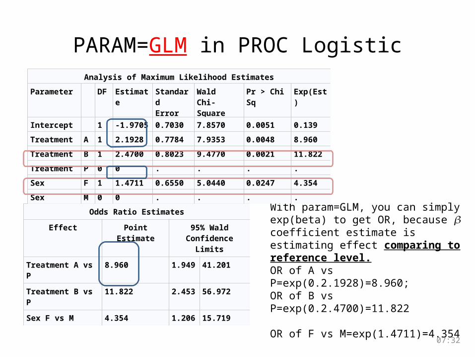
Odds Ratio EstimatesEffect Point Estimate 95% Wald

Confidence LimitsTreatment A vs P 8.960 1.949 41.201Treatment B vs P 11.822 2.453 56.972Sex F vs M 4.354 1.206 15.719

With param=GLM, you can simply exp(beta) to get OR, because 𝛽 coefficient estimate is estimating effect comparing to reference level.OR of A vs P=exp(0.2.1928)=8.960; OR of B vs P=exp(0.2.4700)=11.822

OR of F vs M=exp(1.4711)=4.354

Analysis of Maximum Likelihood Estimates

Parameter   DF Estimate StandardError

WaldChi-Square

Pr > ChiSq Exp(Est)

Intercept   1 -1.9705 0.7030 7.8570 0.0051 0.139

Treatment A 1 2.1928 0.7784 7.9353 0.0048 8.960

Treatment B 1 2.4700 0.8023 9.4770 0.0021 11.822

Treatment P 0 0 . . . .

Sex F 1 1.4711 0.6550 5.0440 0.0247 4.354

Sex M 0 0 . . . .

09:44

PARAM=EFFECT in PROC Logistic

proc logistic data=data1; class Treatment Sex/param=effect;

model Pain= Treatment Sex/ expb; run;

Class Level Information

Class Value Design Variables

Treatment A 1 0

  B 0 1

  P -1 -1

Sex F 1  

  M -1

*Default param=effect*Default reference is “LAST” value. But you can change reference.*There is c-1 column in design matrix, c is the number of level of class var. Reference value coded as -1.

09:44

PARAM=EFFECT in PROC LogisticAnalysis of Maximum Likelihood Estimates

Parameter   DF Estimate StandardError

WaldChi-Square

Pr > ChiSq Exp(Est)

Intercept   1 0.3193 0.3089 1.0685 0.3013 1.376Treatment A 1 0.6385 0.4323 2.1815 0.1397 1.894Treatment B 1 0.9157 0.4467 4.2032 0.0403 2.499Sex F 1 0.7355 0.3275 5.0440 0.0247 2.087

Odds Ratio EstimatesEffect Point Estimate 95% Wald

Confidence LimitsTreatment A vs P 8.960 1.949 41.201Treatment B vs P 11.822 2.453 56.972Sex F vs M 4.354 1.206 15.719

*Normally, one CANNOT calculate OR=exp(beta) in GLM, because 𝛽 coefficient estimate is estimating effect comparing to average of all level.* It is possible that p-value in beta estimate and 95% of OR in OR estimate are NOT consistent

OR of A vs P=exp(2*0.6385+0.9157))=8.960; OR of B vs P=exp(2*0.9157+0.6385))=11.822OR if F vs M=exp(2x0.7355)=4.354 Huh

09:44

PARAM=EFFECT in PROC LogisticAccording to design matrix: treatment=P is coded as -1:

Therefore the logit function of each treatment group, difference between non-ref vs ref, Odds and OR are:

B

A

111001

F

11

Matrix design for treatment Matrix design for sex

Class Logit function Odds difference OR

Trt A L(A)=𝛽0+𝛽A Exp(𝛽0+𝛽A) A vs P: L(A)-L(P)=2𝛽A+𝛽B Exp(2𝛽A+𝛽B)

B L(B)=𝛽0+𝛽B Exp(𝛽0+𝛽B) B vs P: L(B)-L(P)=2𝛽B+𝛽A Exp(2𝛽B+𝛽A)

P L(P)=𝛽0-𝛽A-𝛽B Exp(𝛽0-𝛽A-𝛽B)

Sex F L(F)=𝛽0+𝛽F Exp(𝛽0+𝛽F) F vs M: L(F)-L(M)=2𝛽F Exp(2𝛽F)

M L(M)=𝛽0-𝛽F Exp(𝛽0-𝛽F)

09:44

PARAM=REF in PROC Logistic

• proc logistic data=data1; class Treatment Sex/param=REF;

• model Pain= Treatment Sex/ expb; • run;

*Reference value coded as 0. Class Level Information

Class Value Design Variables

Treatment A 1 0

  B 0 1

  P 0 0

Sex F 1  

  M 0

09:44

PARAM=REF in PROC Logistic

Odds Ratio EstimatesEffect Point Estimate 95% Wald

Confidence LimitsTreatment A vs P 8.960 1.949 41.201Treatment B vs P 11.822 2.453 56.972Sex F vs M 4.354 1.206 15.719

With param=REF, SAS output simply omit reference row, otherwise, estimate values are the same as GLM. OR is calculated in the same way as GLM.

OR of A vs P=exp(2.1928)=8.960; OR of B vs P=exp(2.4700)=11.822

OR of F vs M=exp(1.4711)=4.354

Analysis of Maximum Likelihood Estimates

Parameter   DF Estimate StandardError

WaldChi-Square

Pr > ChiSq Exp(Est)

Intercept   1 -1.9705 0.7030 7.8570 0.0051 0.139

Treatment A 1 2.1928 0.7784 7.9353 0.0048 8.960

Treatment B 1 2.4700 0.8023 9.4770 0.0021 11.822

Sex F 1 1.4711 0.6550 5.0440 0.0247 4.354

09:44

Mixed Coding System in PROC LogisticOne can specify different param option for different class vars, though not usual. Individual parametrization trump global option, unless the global option is GLM.

proc logistic data=data1; class Treatment(param=effect) Sex(param=ref)/param=ref; model Pain= Treatment Sex / expb;run;

Analysis of Maximum Likelihood EstimatesParameter   DF Estimate Standard Error Wald Chi-Square Pr > ChiSq Exp(Est)Intercept   1 -0.4163 0.4252 0.9586 0.3276 0.659Treatment A 1 0.6385 0.4323 2.1815 0.1397 1.894Treatment B 1 0.9157 0.4467 4.2032 0.0403 2.499Sex F 1 1.4711 0.6550 5.0440 0.0247 4.354

Odds Ratio Estimates

Effect Point Estimate 95% WaldConfidence Limits

Treatment A vs P 8.960 1.949 41.201

Treatment B vs P 11.822 2.453 56.972

Sex F vs M 4.354 1.206 15.719

OR of A vs P=exp(2*0.6385+0.9157)=8.960 OR of B vs P=exp(2*0.9175+0.9157)=11.822

OR of F vs M=exp(1.4711)=4.354

09:44

Contrast StatementWhat if I want to compare treatment A vs B, or average A and B vs P, without changing reference group and without rerun the procedure?

The answer is using Contrast statement. However, different coding have profound impact on how to write Contrast statement.

General syntax: CONTRAST 'label' <var-name > <dummy_coeff_1 …dummy_coeffecient_n>/options;

09:44

Contrast Statement with Effect Coding in Logistic

Comparing A vs B: We know L(A)=𝛽0+𝛽A, and L(B)=𝛽0+𝛽B, therefore L(A)-L(B)= 𝛽A - 𝛽B, and we can write contrast statement as:

Contrast “A vs B” treatment 1 -1;

Class Logit function Odds difference OR

Trt A L(A)=𝛽0+𝛽A Exp(𝛽0+𝛽A) A vs P: L(A)-L(P)=2𝛽A+𝛽B Exp(2𝛽A+𝛽B)

B L(B)=𝛽0+𝛽B Exp(𝛽0+𝛽B) B vs P: L(B)-L(P)=2𝛽B+𝛽A Exp(2𝛽B+𝛽A)

P L(P)=𝛽0-𝛽A-𝛽B Exp(𝛽0-𝛽A-𝛽B)

Sex F L(F)=𝛽0+𝛽F Exp(𝛽0+𝛽F) F vs M: L(F)-L(M)=2𝛽F Exp(2𝛽F)

M L(M)=𝛽0-𝛽F Exp(𝛽0-𝛽F)

09:44

Contrast Statement with Effect Coding in Logistic

Contrast Estimation and Testing Results by RowContrast Type Row Estimate Standard

ErrorAlpha Confidence Limits Wald

Chi-SquarePr > ChiSq

A vs B PARM 1 -0.2772 0.7463 0.05 -1.7399 1.1855 0.1380 0.7103A vs B EXP 1 0.7579 0.5656 0.05 0.1755 3.2725 0.1380 0.7103

Analysis of Maximum Likelihood EstimatesParameter   DF Estimate Standard

ErrorWald

Chi-SquarePr > ChiSq Exp(Est)

Intercept   1 0.3193 0.3089 1.0685 0.3013 1.376Treatment A 1 0.6385 0.4323 2.1815 0.1397 1.894Treatment B 1 0.9157 0.4467 4.2032 0.0403 2.499Sex F 1 0.7355 0.3275 5.0440 0.0247 2.087

proc logistic data=data1; class Treatment Sex/param=effect; model Pain= Treatment Sex /e expb; Contrast "A vs B" treatment 1 -1/ e estimate=both;run;

Coefficients of Contrast Avs B

Parameter Row1

TreatmentA 1

TreatmentB -1

09:44

Contrast Statement with Effect Coding in LogisticNow compare average of (A and B) vs P: ½{L(A)+L(B)} - L(P) = 1/2(𝛽0+𝛽A+𝛽0+𝛽B) - (𝛽0-𝛽A-𝛽B) = 1.5𝛽A+1.5 𝛽B

proc logistic data=data1; class Treatment Sex/param=effect; model Pain= Treatment Sex / expb; Contrast “average of (A and B) vs P" treatment 1.5 1.5/ e estimate=both;run;

Coefficients of Contrast average of (A and B) vs PParameter Row1Intercept 0TreatmentA 1.5TreatmentB 1.5

Contrast Estimation and Testing Results by RowContrast Type Row Estimate Standard

ErrorAlpha Confidence Limits Wald

Chi-SquarePr > ChiSq

average of (A and B) vs P PARM 1 2.3314 0.6969 0.05 0.9656 3.6972 11.1931 0.0008average of (A and B) vs P EXP 1 10.2923 7.1722 0.05 2.6263 40.3341 11.1931 0.0008

09:44

Contrast statement Coding in PROC GLM• Unlike proc logistic, GLM coding is the only coding scheme in proc GLM.• Always use the “LAST” value as reference group. A=2 and B=3 in following case.

Example: Y being continuous response following normal distribution with constant variance. The model has two factors, A with 2 levels and B with 3 levels. Main Effect model: Yij = μ + αi + βj + εij, where i is the level of factor A, and j is the level of BThe design matrix of main effect model:

Data Design Matrix

A B

A B 𝜇 (intercept) A1 A2 B1 B2 B3

1 1 1 1 0 1 0 0

1 2 1 1 0 0 1 0

1 3 1 1 0 0 0 1

2 1 1 0 1 1 0 0

2 2 1 0 1 0 1 0

2 3 1 0 1 0 0 1

09:44

Contrast Statement in PROC GLMTest hypothesis 1: H 0 : μ B1 = μ B2

From the design matrix, we know μ B1 = μ + αi + β1 and μ B2 = μ + αi + β2

μ B1 - μ B2 = β1 -β2

Contrast statement: Contrast “B=1 vs B=2” B 1 -1 / e proc glm data=data3;

class a b;model y=a b/solution;contrast "B=1 vs B=2" B 1 -1/e;ESTIMATE "B=1 vs B=2" B 1 -1/e; *Usually Contrast and Esitmate go hand-in-hand,

Esitmate give estimate of difference and SE

run;Contrast DF Contrast SS Mean Square F Value Pr > FB=1 vs B=2 1 4.98877622 4.98877622 4.85 0.0328

Parameter Estimate Standard Error t Value Pr > |t|B=1 vs B=2 -0.84927549 0.38544563 -2.20 0.0328

09:44

Contrast Statement Coding in PROC GLMModel with crossed effects: Yijk = μ + αi + βj + αβij + εijk , where i is the level of factor A, and j is the level of B, and k is level of A*B

The design matrix of crossed effect model:

Data Design Matrix

A B A*B

A B μ A1 A2 B1 B2 B3 A1B1

A1B2

A1B3

A2B1

A2B2

A2B3

1 1 1 1 0 1 0 0 1 0 0 0 0 0

1 2 1 1 0 0 1 0 0 1 0 0 0 0

1 3 1 1 0 0 0 1 0 0 1 0 0 0

2 1 1 0 1 1 0 0 0 0 0 1 0 0

2 2 1 0 1 0 1 0 0 0 0 0 1 0

2 3 1 0 1 0 0 1 0 0 0 0 0 1

09:44

Contrast Statement in PROC GLMTest hypothesis 2: H 0 : μ𝛼B11 = μ𝛼B12

From the design matrix, we know: μ𝛼B11 = μ + α1 + β1 + αβ11 and μ𝛼B12= μ + α1 + β2 + αβ12

μ B1 - μ B2 = β1 -β2+ αβ11- αβ12

Contrast statement: now have two dummy coefficientsproc glm data=data3;

class a b;model y=a b/solution;contrast "B=1 vs B=2" B 1 -1

A*B 1 -1; *This is equivalent as 1 -1 0 0 0 0 , trailing 0 can be ignored;

ESTIMATE "B=1 vs B=2" B 1 -1; A*B 1 -1;

run;Contrast DF Contrast SS Mean Square F Value Pr > F

AB11 vs AB12 1 6.81411446 6.81411446 6.53 0.0143

Parameter Estimate Standard Error t Value Pr > |t|

AB11 vs AB12 -1.40976950 0.55182283 -2.55 0.0143

09:44

Steps to Construct Contrast Statement

Step 1. Write down the model, two crucial parts to this. – Parameterization: how design variables in class statement

are coded.– Parameter ordering: the order of parameters depends on

class statement and order option. Confirm from SAS output.

Step 2. Write down the hypothesis to be tested.Step 3. Write the CONTRAST.

09:44

Default and Alternative Coding in Regression SAS Procedures

Default design matrix coding Regression proceduresGLM coding (indicator or dummy): ref value coded as 1

GENMOD, GLM, GLMSELECT, GLIMMIX, LIFEREG, MIXED, and SURVEYPHREG

EFFECT coding (deviation from mean) : ref value coded as -1

CATMOD, LOGISTIC, and SURVEYLOGISTIC

REF coding: ref value coded as 0 PHREG and TRANSREG

Alternative coding allowed? Regression proceduresAllowed LOGISTIC, GENMOD, GLMSELECT, PHREG,

SURVEYLOGISTIC, and SURVEYPHREG.

Not allowed GLM, MIXED, GLIMMIX, and LIFEREG

09:44

Take Home Messages• Design matrix has profound impact on CONTRAST/LSMEAN statement and

result interpretation. • First, know the design matrix you are using and true math linear

combination of the matrix.• The variables order in class statement matters.• Effect coding is estimating effect comparing to average of all level, not to

the reference.• Follow steps of constructing contrast statement:

– Step 1: know the design matrix and order of parameters– Step 2: Write done the hypothesis tests– Step 3: Construct contrast and ESTIMATE statement

• Different regression procedures have different default design matrix schemes, and not all procedure allows alternative schemes.

09:44

Acknowledgement

• Thanks Kathy Roggenkamp for your encouragement and support!

09:44