Design Hydrology and Sedimentation for Small · PDF fileFrom Haan et al. 1994. Design Hydrology and Sedimentation for Small Catchments. Academic Press, New York, pp. 588

From Haan et al. 1994. Design Hydrology and Sedimentation for Small Catchments. Academic Press, New York, pp. 588.

BEE 473 Watershed Engineering Fall 2007

October 17, 2008

IMPOUNDMENTS (PONDS, WETLANDS, RESERVOIRS, AND DETENTION BASINS) Designing ponds and detention basins and similar impoundments requires engineers to keep track of stored water during a storm; most or our previous designs have only required that the structure or system have a capacity greater than the peak discharge. Because of this, we often design ponds and detention basins for large volume storms as well as high intensity storms. The synthetic hydrograph approaches you have been using are only valid for storms with durations similar to a watershed’s time of concentration. Typically detention basin and similar structures are designed for a 24-hr storm, which will require some extra calculations. Ponds, detention basins, etc. typically consist of a pool for storing water, a mechanical spillway for controlling outflow, and an emergency or auxiliary spillway for events exceeding the design so that the structure is not destroyed; you know how to design most of these components already. The following will provide additional information needed.

A. Level-Pool Flood RoutingB. Triangular Hydrograph SuperpositionC. Synthetic Unit Hydrograph D. Embankment Design


A. Level-Pool Flood Routing Level-pool flood routing is a simple step-wise mass balance that allows engineers to simultaneously estimate of outflow and storage from a pond or similar structure that is receiving variable inflow, usually described by a hydrograph. The first step is to determine your inflow hydrograph and divide it into small time increments, ∆t, such that ∆t ≤ tp/10. IMPORTANT: Use this ∆t throughout the rest of the analysis. In essence, level-pool flood routing uses the fact that outflow and storage are both function of the water depth in the pond so that we can combine inflow and storage into a single function.

( )Hft

So=⎟

⎠⎞

⎜⎝⎛

∆+

2 (A.1)

where o is outflow discharge (m3 s-1), S is flood storage in the pond (m3), and ∆t is in seconds. Determine relationship by guessing the dimensions of the pond and outflow structure (e.g., a 1 m deep oval pond with a 5 m long, 10 cm dia. culvert with a1% slope) and calculating the outflow discharge and storage volume for a range of depths, H. For the subsequent analysis it is easiest to consider the relationship between the left-hand side of Eq. (A.1) and outflow:

⎟⎠⎞

⎜⎝⎛

∆+=

tSofo

2 (A.2)

Sometimes you will find that a continuous function describes (A.2) and can be used through the rest of the analysis. The mass balance for the pond can be written in the following form.

tt

ttt

tt

ot

Soiit

So−⎟

⎠⎞

⎜⎝⎛

∆++

+=⎟

⎠⎞

⎜⎝⎛

∆+ ∆+

∆+ 222 (A.3)

Assuming that at t = 0, outflow and storage are zero, the following table illustrates how to proceed with flood routing. known known known Eq. A.3 Eq. A.2

t i 2

ttt ii ∆++

tSo∆

+2

o

0 io (io+ i1)/2 0 0 ∆t i1 (i1+ i2)/2 (io+ i1)/2+0-0 Eq. A.2 2∆t i2 (i2+ i3)/2 Repeat Repeat ↓ ↓ ↓ ↓ ↓

n∆t 0 0 on


B. Triangular Hydrograph Superposition Perhaps the simplest way to approximate a hydrograph for a long storm is to divide the storm into periods with duration equal to the time of concentration, use a triangular hydrograph to approximate the flow from each sub-storm, and then superimpose them as shown in Fig. B.1

Composite hydrograph

time

disc

harg

era

in

~ tc

Composite hydrograph

time

disc

harg

era

in

~ tc

Figure B.1: Illustration of a composite hyetograph (top) and hydrograph (bottom) constructed by superimposing three SCS-triangular hydrographs.


C. Synthetic Unit Hydrograph The unit hydrograph concept was first developed in the 1930’s by L.K. Sherman. As illustrated in Fig. C.1, the unit hydrograph assumes that for a given uniform input of rain over a specific duration, ∆D, that generates in a unit, e.g., 1 mm, (1 inch in English units) of runoff (also called precipitation excess), a watershed will produce a characteristic runoff outflow response or unit hydrograph. In other words, if the watershed experiences a 1 mm slug or pulse of runoff, the unit hydrograph describes how fast that runoff reaches to the watershed outlet.

t/tp

1 2

0.25

3

0.50

4

0.75

1.00

qu/qpWatershed Outflow

1.00

Run

off

Dep

th Total Runoff(a.k.a. Excess Precipitation)

0.00

0.00

rain Don’t worry about amount, just

be cognizant of that its duration, ∆D, is <tc (e.g. ∆D˜ 0.133tc)0.00

∆D

t/tp

1 2

0.25

3

0.50

4

0.75

1.00


1.00

Run

off

Dep


0.00

0.00



∆D

Figure C.1: Schematic of the unit hydrograph concept – the axes have been normalized for

illustration purposes. Here, qu is the unit hydrograph The primary assumption that makes the unit hydrograph useful is that the watershed is a linear system; that is, (1) the unit hydrograph obeys the principle of proportionality and (2) multiple unit hydrographs can be superimposed. Thus, considering the proportionality of the unit hydrograph, if the watershed experiences a rainfall event of duration ∆D that produces 2 mm of runoff (i.e., twice the unit hydrograph), the response or resulting hydrograph, q(t), is determined by doubling qu for all times. The ability to superpose unit hydrographs is essential to capture hydrograph responses to long storms when rainfall rates may be non-uniform. For instance, if 2 mm of runoff occurred over two consecutive periods of ∆D (each generating 1 mm of runoff), the resulting response or hydrograph is determined by creating independent hydrographs for each runoff event (in this case the unit hydrograph is multiplied by “one” for each event) and superimposing them on each other as illustrated in Fig. C2. Note, it might be tempting to simply double the response time following the logic that qp doubles when runoff doubles for an event of duration ∆D. However the times at which runoff reaches the outlet is largely controlled by the time of concentration, tc, which is an innate physical characteristic of the watershed that does not change from storm to storm.


t/tp

1 2

0.25

3

0.50

4

0.75

1.00

q/qp

SuperimposedWatershed Outflow

1.00

Run

off

Dep

th

Two Runoff Pulses generated by two rainfall pulses of ∆D.

0.00

0.00

t/tp

1 2

0.25

3

0.50

4

0.75

1.00

q/qp


1.00

Run

off

Dep

th


0.00

0.00

Figure 2.C: Illustration of using superposition to create a composite hydrograph from two consecutive unit runoff impulses – the axes have been normalized for illustration purposes.

An important aspect of using unit hydrographs is deciding on the duration of rainfall excess, ∆D (Fig. C.1). One standard calculation of rainfall excess duration is: 133.0×=∆ ctD (NEH, Eqn 6.12 -- Chapter 16 of NEH includes an example illustrating the effects of using too large a ∆D). Remember that a long storm will be composed of multiple rainfall-runoff pulses of duration ∆D; the storm length will, in most cases, not be ∆D. Another complication is determining tp for a storm of duration ∆D. A commonly used calculation is:

cp tDt 6.02

+∆

= (C.0)

Note, this is consistent with the approximation we use when we are developing a hydrograph for a design storm that will produce the maximum peak runoff rate, i.e., when the duration of the storm is equal to the tc; i.e., if ∆D = tc then Eq. C.0 becomes tp = 1.1tc. Figures C.1 and C.2 show curvy unit hydrographs because sometimes the unit hydrograph is determined from actual storm discharge data generated by an actual storm of duration ∆D. Later we will discuss using synthetic hydrographs. Quantification of Unit Hydrograph Thus far, we have kept the unit hydrograph discussion descriptive. It is relatively easy to use the unit hydrograph concept to develop a hydrograph for a long, perhaps non-uniform rainfall event by (1) dividing the long storm into many uniform mini-rainfall events of duration ∆D, (2) calculating the runoff from each mini-rainfall event, (3) scaling the unit hydrograph for each runoff pulse, and (4) superimposing all the resulting hydrographs. Indeed, there is nothing wrong with this approach.


The following is a more computationally efficient way to do this. The basic equation used is referred to as the discrete convolution equation (equivalent to the convolution integral used in continuous calculations):

(C.1) ∑=

+−=n

mmnmm UQq

11

where q is the runoff outflow rate, Q is the runoff depth generated by a precipitation event of duration ∆D, U is a response function (unit hydrograph, essentially qu in Fig. C.1), m is the time interval, and. n is the number of intervals in the response function plus the number of input pulses minus 1. Example: Consider the response function in Table C.1 and the input pulses summarized in Table C.2. Note n = 5+3-1, n = 7

Table C.1: Response Function Unit Time U

1 0.05 2 0.1 3 0.6 4 0.2 5 0.15

Table C.2: Runoff Pulse Unit Time Q

1 0.5 2 1.5 3 1

At m = 1, q1=Q1U1 or q1 = 0.5x0.05 = 0.025.

At m = 2, q2 = Q1U2 + Q2U1 or q2 = 0.5x0.1 + 1.5x0.05 = 0.125 ↓ ↓

At m = 5, q5 = Q1U5 + Q2U4+ Q3U3 or q5 = 0.5x0.15+1.5x0.2+1x0.6 = 0.975 ↓ ↓

This process is repeated to m = 7. The runoff outflow at distinct time intervals is given by the series of quantities q1 to q7. Synthetic Unit Hydrograph The unit hydrograph concept allows that each watershed has a unique response to a storm. Because it is not always tenable to develop unique unit hydrographs for every watershed, which would require simultaneous streamflow and rainfall measurements over a prolonged period, synthetic unit hydrographs have been developed by, the Soil Conservation Service (SCS – currently the Natural Resources Conservation Service or NRCS) using compiled data from multiple watersheds. One of these is the triangular unit hydrograph we have used earlier in this class, which can be used to develop a synthetic unit hydrograph with a tp determined by Eq. C.0 (i.e., tp = ∆D/2+0.6tc where ∆D << tc) and the volume of runoff equal to 1-mm over the watershed area (the recession time, tr, is still 1.67tp). Using the tp and qp from a synthetic triangular unit hydrograph, you can create a more curvy synthetic unit hydrograph by multiplying these values by the appropriate ordinates of the dimensionless synthetic hydrograph given on an attached sheet (i.e., by multiplying the y-axes by qp and the x-axis by tp). In many design cases engineers use the SCS synthetic unit hydrograph, largely because it is embedded in commonly used watershed design software.


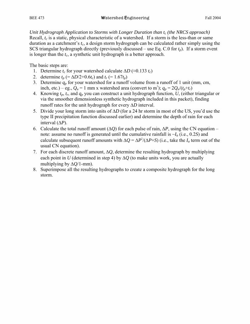
Unit Hydrograph Application to Storms with Longer Duration than tc (the NRCS approach) Recall, tc is a static, physical characteristic of a watershed. If a storm is the less-than or same duration as a catchment’s tc, a design storm hydrograph can be calculated rather simply using the SCS triangular hydrograph directly (previously discussed – use Eq. C.0 for tp). If a storm event is longer than the tc, a synthetic unit hydrograph is a better approach. The basic steps are:

1. Determine tc for your watershed calculate ∆D (≈0.133 tc) 2. determine tp (= ∆D/2+0.6tc) and tr (= 1.67tp) 3. Determine qp for your watershed for a runoff volume from a runoff of 1 unit (mm, cm,

inch, etc.) – eg., Qu = 1 mm x watershed area (convert to m3); qp = 2Qu/(tp+tr) 4. Knowing tp, tr, and qp you can construct a unit hydrograph function, U, (either triangular or

via the smoother dimensionless synthetic hydrograph included in this packet), finding runoff rates for the unit hydrograph for every ∆D interval.

5. Divide your long storm into units of ∆D (for a 24 hr storm in most of the US, you’d use the type II precipitation function discussed earlier) and determine the depth of rain for each interval (∆P).

6. Calculate the total runoff amount (∆Q) for each pulse of rain, ∆P, using the CN equation – note: assume no runoff is generated until the cumulative rainfall is ~Ia (i.e., 0.2S) and calculate subsequent runoff amounts with ∆Q = ∆P2/(∆P+S) (i.e., take the Ia term out of the usual CN equation).

7. For each discrete runoff amount, ∆Q, determine the resulting hydrograph by multiplying each point in U (determined in step 4) by ∆Q (to make units work, you are actually multiplying by ∆Q/1-mm).

8. Superimpose all the resulting hydrographs to create a composite hydrograph for the long storm.


D. Embankment Design Figure D.1 shows the various dimensions that need to be determined when designing an earth embankment; K is the hydraulic conductivity of the embankment material. One of the primary design constraints, especially if the embankment is supposed to impound a permanent water body, is the seepage through the structure, q. The downstream toe should be outfitted with a drain to remove this water. If the available material for embankment construction is too permeable, a clay core can be constructed assuming the same relationships as shown in Fig. D.1.

LKHq9

4 2

=

α

( )αcot6H

3H

H

M L

0.3M

su

sd

hf

wt

Actual water surface

Approximate water surface

LKHq9

4 2

=

α

( )αcot6H

3H

H

M L

0.3M

su

sd

hf

wt

Actual water surface

Approximate water surface

Figure D.1: Schematic of embankment cross-section and relevant design dimensions The slope of upstream face, su, should not generally not exceed 1:3; <1:4 if the embankment material is coarse and <1:7 for uncompacted material such as in levees. The slope of downstream face, sd, should not generally not exceed 1:2; <1:3 if the embankment material is coarse and <1:7 for uncompacted material such as in levees. The upstream and downstream faces can have slopes up to 1:1 if the seepage section is a core embedded in a larger dam. The freeboard height, hf, is often estimated as 0.014(fetch)1/2; all units are meters and fetch is the unobstructed upwind distance above the dam. The top width, wt, should be at least 2.4 m and for H > 3.5 m the minimum wt can be estimated as 0.4H+1; all units are meters. Allow 5-10% settling height in general and 20 – 25% for levees.


References: National Engineering Handbook (NEH). 1972. Dean Snider. Part 630: Hydrology. Chapter 16-

Hydrographs. NRCS. website: http://www.nrcs.usda.gov/technical/ENG/neh.html For further information: *Chow, V.T. 1959. Open Channel Hydraulics. McGraw-Hill Company, New York. pp. 680. †Haan, C.T., B.J. Barfield, J.C. Hayes. 1994. Design Hydrology and Sedimentology for Small

Catchments. Academic Press, New York. pp. 588. *Montes, S. Hydraulics of Open Channel Flow. ASCE Press, Reston. pp. 697. †Schwab, G.O., D.D. Fangmeier, W.J. Elliot, R.K. Frevert. 1993. Soil and Water Conservation

Engineering, 4th Ed. John Wiley & Sons, Inc. New York. pp.508. †Tollner, E.W. 2002. Natural Resources Engineering. Iowa State Press, Ames. pp. 576. * Particularly good books for open channels † These texts were previously used for this course


References: National Engineering Handbook (NEH). 1972. Dean Snider. Part 630: Hydrology. Chapter 16-Hydrographs. NRCS. Website: www.nrcs.usda.gov/technical/ENG/neh.html. For further information: Chin, D.A. Water Resources Engineering. Prentice Hall. Upper Saddle River. pp. 750. *Chow, V.T. 1959. Open Channel Hydraulics. McGraw-Hill Company, New York. pp. 680. †Haan, C.T., B.J. Barfield, J.C. Hayes. 1994. Design Hydrology and Sedimentology for Small

Catchments. Academic Press, New York. pp. 588. †Schwab, G.O., D.D. Fangmeier, W.J. Elliot, R.K. Frevert. 1993. Soil and Water Conservation

Engineering, 4th Ed. John Wiley & Sons, Inc. New York. pp.508. †Tollner, E.W. 2002. Natural Resources Engineering. Iowa State Press, Ames. pp. 576. * Particularly good books for this topic † These texts were previously used for this course


C. Synthetic Unit Hydrograph The unit hydrograph concept was first developed in the 1930’s by L.K. Sherman. As illustrated in Fig. C.1, the unit hydrograph assumes that for a given uniform input of rain over a specific duration, ∆D, that generates in a unit, e.g., 1 mm, (1 inch in English units) of runoff (also called precipitation excess), a watershed will produce a characteristic runoff outflow response or unit hydrograph. In other words, if the watershed experiences a 1 mm slug or pulse of runoff, the unit hydrograph describes how fast that runoff reaches to the watershed outlet.

t/tp

1 2

0.25

3

0.50

4

0.75

1.00


1.00

Run

off

Dep


0.00

0.00



∆D

t/tp

1 2

0.25

3

0.50

4

0.75

1.00


1.00

Run

off

Dep


0.00

0.00



∆D

Figure C.1: Schematic of the unit hydrograph concept – the axes have been normalized for

illustration purposes. Here, qu is the unit hydrograph The primary assumption that makes the unit hydrograph useful is that the watershed is a linear system; that is, (1) the unit hydrograph obeys the principle of proportionality and (2) multiple unit hydrographs can be superimposed. Thus, considering the proportionality of the unit hydrograph, if the watershed experiences a rainfall event of duration ∆D that produces 2 mm of runoff (i.e., twice the unit hydrograph), the response or resulting hydrograph, q(t), is determined by doubling qu for all times. The ability to superpose unit hydrographs is essential to capture hydrograph responses to long storms when rainfall rates may be non-uniform. For instance, if 2 mm of runoff occurred over two consecutive periods of ∆D (each generating 1 mm of runoff), the resulting response or hydrograph is determined by creating independent hydrographs for each runoff event (in this case the unit hydrograph is multiplied by “one” for each event) and superimposing them on each other as illustrated in Fig. C2. Note, it might be tempting to simply double the response time following the logic that qp doubles when runoff doubles for an event of duration ∆D. However the times at which runoff reaches the outlet is largely controlled by the time of concentration, tc,

October 17, 2008


which is an innate physical characteristic of the watershed that does not change from storm to storm.

t/tp

1 2

0.25

3

0.50

4

0.75

1.00

q/qp


1.00

Run

off

Dep

th


0.00

0.00

t/tp

1 2

0.25

3

0.50

4

0.75

1.00

q/qp


1.00

Run

off

Dep

th


0.00

0.00

Figure 2.C: Illustration of using superposition to create a composite hydrograph from two consecutive unit runoff impulses – the axes have been normalized for illustration purposes.

An important aspect of using unit hydrographs is deciding on the duration of rainfall excess, ∆D (Fig. C.1). One standard calculation of rainfall excess duration is: 133.0×=∆ ctD (NEH, Eqn 6.12 -- Chapter 16 of NEH includes an example illustrating the effects of using too large a ∆D). Remember that a long storm will be composed of multiple rainfall-runoff pulses of duration ∆D; the storm length will, in most cases, not be ∆D. Another complication is determining tp for a storm of duration ∆D. A commonly used calculation is:

cp tDt 6.02

+∆

= (C.0)

Note, this is consistent with the approximation we use when we are developing a hydrograph for a design storm that will produce the maximum peak runoff rate, i.e., when the duration of the storm is equal to the tc; i.e., if ∆D = tc then Eq. C.0 becomes tp = 1.1tc. Figures C.1 and C.2 show curvy unit hydrographs because sometimes the unit hydrograph is determined from actual storm discharge data generated by an actual storm of duration ∆D. Later we will discuss using synthetic hydrographs. Quantification of Unit Hydrograph Thus far, we have kept the unit hydrograph discussion descriptive. It is relatively easy to use the unit hydrograph concept to develop a hydrograph for a long, perhaps non-uniform rainfall event by (1) dividing the long storm into many uniform mini-rainfall events of duration ∆D, (2) calculating the runoff from each mini-rainfall event, (3) scaling the unit hydrograph for each


runoff pulse, and (4) superimposing all the resulting hydrographs. Indeed, there is nothing wrong with this approach. The following is a more computationally efficient way to do this. The basic equation used is referred to as the discrete convolution equation (equivalent to the convolution integral used in continuous calculations):

(C.1) ∑=

+−=n

mmnmm UQq

11

where q is the runoff outflow rate, Q is the runoff depth generated by a precipitation event of duration ∆D, U is a response function (unit hydrograph, essentially qu in Fig. C.1), m is the time interval, and. n is the number of intervals in the response function plus the number of input pulses minus 1. Example: Consider the response function in Table C.1 and the input pulses summarized in Table C.2. Note n = 5+3-1, n = 7

Table C.1: Response Function Unit Time U

1 0.05 2 0.1 3 0.6 4 0.2 5 0.15

Table C.2: Runoff Pulse Unit Time Q

1 0.5 2 1.5 3 1

At m = 1, q1=Q1U1 or q1 = 0.5x0.05 = 0.025.

At m = 2, q2 = Q1U2 + Q2U1 or q2 = 0.5x0.1 + 1.5x0.05 = 0.125 ↓ ↓

At m = 5, q5 = Q1U5 + Q2U4+ Q3U3 or q5 = 0.5x0.15+1.5x0.2+1x0.6 = 0.975 ↓ ↓

This process is repeated to m = 7. The runoff outflow at distinct time intervals is given by the series of quantities q1 to q7. Synthetic Unit Hydrograph The unit hydrograph concept allows that each watershed has a unique response to a storm. Because it is not always tenable to develop unique unit hydrographs for every watershed, which would require simultaneous streamflow and rainfall measurements over a prolonged period, synthetic unit hydrographs have been developed by, the Soil Conservation Service (SCS – currently the Natural Resources Conservation Service or NRCS) using compiled data from multiple watersheds. One of these is the triangular unit hydrograph we have used earlier in this class, which can be used to develop a synthetic unit hydrograph with a tp determined by Eq. C.0 (i.e., tp = ∆D/2+0.6tc where ∆D << tc) and the volume of runoff equal to 1-mm over the watershed area (the recession time, tr, is still 1.67tp). Using the tp and qp from a synthetic triangular unit hydrograph, you can create a more curvy synthetic unit hydrograph by multiplying these values by the appropriate ordinates of the dimensionless synthetic hydrograph given on an attached sheet (i.e., by multiplying the y-axes by qp and the x-axis by tp). In many design cases engineers use the SCS synthetic unit hydrograph, largely because it is embedded in commonly used watershed design software.


Unit Hydrograph Application to Storms with Longer Duration than tc (the NRCS approach) Recall, tc is a static, physical characteristic of a watershed. If a storm is the less-than or same duration as a catchment’s tc, a design storm hydrograph can be calculated rather simply using the SCS triangular hydrograph directly (previously discussed – use Eq. C.0 for tp). If a storm event is longer than the tc, a synthetic unit hydrograph is a better approach. The basic steps are:

1. Determine tc for your watershed calculate ∆D (≈0.133 tc) 2. determine tp (= ∆D/2+0.6tc) and tr (= 1.67tp) 3. Determine qp for your watershed for a runoff volume from a runoff of 1 unit (mm, cm,

inch, etc.) – eg., Qu = 1 mm x watershed area (convert to m3); qp = 2Qu/(tp+tr) 4. Knowing tp, tr, and qp you can construct a unit hydrograph function, U, (either triangular or

via the smoother dimensionless synthetic hydrograph included in this packet), finding runoff rates for the unit hydrograph for every ∆D interval.

5. Divide your long storm into units of ∆D (for a 24 hr storm in most of the US, you’d use the type II precipitation function discussed earlier) and determine the depth of rain for each interval (∆P).

6. Calculate the total runoff amount (∆Q) for each pulse of rain, ∆P, using the CN equation – note: assume no runoff is generated until the cumulative rainfall is ~Ia (i.e., 0.2S) and calculate subsequent runoff amounts with ∆Q = ∆P2/(∆P+S) (i.e., take the Ia term out of the usual CN equation).

7. For each discrete runoff amount, ∆Q, determine the resulting hydrograph by multiplying each point in U (determined in step 4) by ∆Q (to make units work, you are actually multiplying by ∆Q/1-mm).

8. Superimpose all the resulting hydrographs to create a composite hydrograph for the long storm.

Documents

Design Hydrology and Sedimentation for Small · PDF fileFrom Haan et al. 1994. Design Hydrology and Sedimentation for Small Catchments. Academic Press, New York, pp. 588